
This PDF is a selection from an out-of-print volume from... of Economic Research
This PDF is a selection from an out-of-print volume from the National Bureau
of Economic Research
Volume Title: A Retrospective on the Bretton Woods System: Lessons for
International Monetary Reform
Volume Author/Editor: Michael D. Bordo and Barry Eichengreen, editors
Volume Publisher: University of Chicago Press
Volume ISBN: 0-226-06587-1
Volume URL: http://www.nber.org/books/bord93-1
Conference Date: October 3-6, 1991
Publication Date: January 1993
Chapter Title: The Bretton Woods International Monetary System: A Historical
Overview
Chapter Author: Michael D. Bordo
Chapter URL: http://www.nber.org/chapters/c6867
Chapter pages in book: (p. 3 - 108)
1
The Bretton Woods International
Monetary System: A Historical
Overview
Michael D. Bordo
After twenty years of floating exchange rates, there is now considerable interest, among those concerned over its perceived shortcomings, in an eventual
return by the world to a fixed exchange rate regime. This interest has been
enhanced by the apparent success of the European Monetary System (EMS)
and the prospects for European monetary unification. The Bretton Woods system was the world’s most recent experiment with a fixed exchange rate regime. Although it was originally designed as an adjustable peg, it evolved in
its heyday into a de fact0 fixed exchange rate regime. That regime ended with
the closing by President Richard Nixon of the gold window on 15 August
1971. Twenty years after that momentous decision, a retrospective look at the
performance of the Bretton Woods system is timely.
This paper presents an overview of the Bretton Woods experience. I analyze
the system’s performance relative to earlier international monetary regimesas well as to the subsequent one-and also its origins, operation, problems,
and demise. In the survey, I discuss issues deemed important during the life
of Bretton Woods and some that speak to the concerns of the present. The
survey is limited to the industrial countries-the G10 and especially the G7. I
do not examine the role of the International Monetary Fund (IMF), the fundamental organization of Bretton Woods, in the economies and international
economic relations of the developing nations.
Section 1.1 compares the macro performance of Bretton Woods with the
preceding and subsequent monetary regimes. The descriptive statistics on
Michael D. Bordo is professor of economics at Rutgers University and a research associate of
the National Bureau of Economic Research.
For helpful comments and suggestions the author would like to thank Forrest Capie, Max Corden, Barry Eichengreen, Lars Jonung, Charles Kindleberger, Adam Klug, Allan Meltzer, Donald
Moggridge, Hugh Rockoff, Anna Schwartz, Leland Yeager, and the NBER conference participants. His thanks for providing data on Japan go to James Lothian and Robert Rasche. Valuable
research assistance has been provided by Bernhard Eschweiller and Johan Koenes.
3
4
Michael D. Bordo
nine key macro variables point to one incontrovertible conclusion. Both nominal and real variables exhibited the most stable behavior in the past century
under the Bretton Woods system, in its full convertibility phase, 1959-71.
While Bretton Woods was relatively stable, it was also very short lived. From
the declaration of par values by thirty-two countries on 18 December 1946 to
the closing of the gold window on 15 August 1971, it lasted twenty-five
years.’ However, most analysts would agree that, until the Western European
industrial countries made their currencies convertible on 27 December 1958,
the system did not operate as intended. On this calculation, the regime lasted
only twelve years. Alternatively, if we date its termination at the end of the
Gold Pool and the start of the two-tier system on 15 March 1968, it was in full
operation only nine years.
This raises questions about why Bretton Woods was statistically so stable
and why it was so short lived. (1) Was Bretton Woods successful in producing
economic stability because it operated during a period of economic stability,
or did the existence of the adjustable peg regime produce economic stability?
Alternatively, was its statistical stability an illusion-belied by the presence
of continual turmoil in the foreign exchange markets? (2) Why did the system
crumble after 1968 and end (so far) irrevocably in August 1971? It is the hope
of the conference organizers that answers to these questions and many others
can be provided by this and other papers to be presented here.
Section 1.2 surveys the origins of Bretton Woods: the perceived problems
of the interwar period; the plans for a new international monetary order; and
the steps leading to the adoption of the Articles of Agreement.
Section 1.3 examines the preconvertibility period from 1946 to 1958, the
problems in getting started exemplified by the dollar shortage and the weakness of the IMF, and the transition of the system to convertibility and the gold
dollar standard.
Section 1.4 analyzes the heyday of Bretton Woods from 1959 to 1967 in the
context of the gold dollar standard and its famous three problems: adjustment,
liquidity, and confidence. I review both the problems and the many proposals
for monetary reform.
Section 1.5 considers the emergence of a “de facto” dollar standard in 1968
and its collapse in the face of U.S.-induced inflation.
Finally, section 1.6 summarizes the main points of the paper, discusses
some lessons learned from the Bretton Woods experience for the design of a
fixed exchange rate regime, and raises questions answered by the other papers
in the conference volume.
1. The par value system was preserved by the Smithsonian Agreement, 18 December 1971,
until its final abandonment on 1 March 1973.
5
The Bretton Woods International Monetary System
1.1 The Performance of Bretton Woods in Comparison to Alternative
Monetary Regimes
The architects of the Bretton Woods system wanted a set of monetary arrangements that would combine the advantage of the classical gold standard
(i.e., exchange rate stability) with the advantage of floating rates (i.e., independence to pursue national full employment policies). They sought to avoid
the defects of floating rates (destabilizing speculation and competitive beggarthy-neighbor devaluations) and the defects of the fixed exchange rate gold
standard (subordination of national monetary policies to the dictates of external balance and subjection of the economy to the international transmission of
the business cycle). As a consequence, they set up an adjustable peg system
of fixed parities that could be changed only in the event of a fundamental
disequilibrium.
The architects derived their views of an ideal international monetary arrangement from their perception of the performance of the pre-World War I
classical gold standard and of the sequence of floating rates and gold exchange
standard that characterized the interwar period. As background to the historical survey of Bretton Woods, I compare descriptive evidence on the macro
performance of the international monetary regime of Bretton Woods with that
on the performance of preceding and subsequent regimes. The comparison for
the seven largest (non-Communist) industrialized countries (the United States,
the United Kingdom, Germany, France, Japan, Canada, and Italy) is based on
annual data for Bretton Woods (1946-70), the present regime of floating rates
(1974-89), and the two regimes preceding Bretton Woods: the interwar period (1919-39) and the classical gold standard (1881-1913). The Bretton
Woods period (1946-70) is divided into two subperiods: the preconvertible
phase (1946-58) and the convertible phase (1959-70).* The comparison also
relates to the theoretical issues raised by the perennial debate over fixed versus
flexible exchange rates. According to the traditional view, adherence to a
(commodity-based) fixed exchange rate regime, such as the gold standard,
ensured long-run price stability for the world as a whole because the fixed
price of gold provided a nominal anchor to the world money supply. By pegging their currencies to gold, individual nations fixed their price levels to that
of the world. The disadvantage of fixed rates is that individual nations were
exposed to both monetary and real shocks transmitted from the rest of the
world via the balance of payments and other channels of transmission (Bordo
and Schwartz 1989). Also, the common world price level under the gold standard exhibited secular periods of deflation and inflation reflecting shocks to
the demand for and supply of gold (Bordo 1981; Rockoff, 1984). However, a
2. I also examined the period 1946-73, which includes the three years of transition from the
Bretton Woods adjustable peg to the present floating regime. The evidence is similar to that of the
period 1946-70, so it is not presented here.
6
Michael D. Bordo
well-designed monetary rule could avoid the long-run swings that characterized the price level under the gold standard (Cagan 1984). The advantage of
floating exchange rates is to provide insulation from foreign shocks. The disadvantage is the absence of the discipline of the fixed exchange rate rulemonetary authorities could follow inflationary policies.
Theoretical developments in recent years have complicated the simple distinction between fixed and floating rates. In the presence of capital mobility,
currency substitution, policy reactions, and policy interdependence, floating
rates no longer necessarily provide insulation from either real or monetary
shocks (Bordo and Schwartz 1989). Moreover, according to recent real business cycle approaches, there may be no relation between the international
monetary regime and the transmission of real shocks (Baxter and Stockman
1989). Neveriheless, the comparison between regimes may shed light on these
issues,
One important caveat is that the historical regimes presented here do not
represent clear examples of fixed and floating rate regimes. The interwar period is composed of three regimes: general floating from 1919 to 1925, the
gold exchange standard from 1926 to 193 1, and a managed float to 1939.3The
Bretton Woods regime cannot be characterized as a fixed exchange rate regime
throughout its history: the preconvertibility period was close to the adjustable
peg envisioned by its architects; the convertible period was close to a de facto
fixed dollar ~ t a n d a r dFinally,
.~
although the period since 1973 has been characterized as a floating exchange rate regime, at various times it has experienced varying degrees of management.
Table 1 . 1 presents descriptive statistics on nine macro variables for each
country, the data for each variable converted to a continuous annual series
from 1880 to 1989. The nine variables are the rate of inflation, real per capita
growth, money growth, short- and long-term nominal interest rates, shortand long-term real interest rates, and the absolute rates of change of nominal
and real exchange rates. The definition of the variable used (e.g., M1 vs. M2)
was dictated by the availability of data over the entire period. For each variable and each country, I present two summary statistics: the mean and the
standard deviation. For inflation, I also show (in parentheses) the standard
deviation of the forecast error based on a univariate regression. For all the
countries taken as a group, I show two summary statistics: the grand mean
and a simple measure of convergence measured as the mean of the absolute
differences between each country’s summary statistic and the grand means of
the group of c o u n t r i e ~I. ~comment on the statistical results for each variable.
3. To be more exact, the United States stayed on the gold standard until 1933 and France until
1936. For a detailed comparison of the performances of these three regimes in the interwar period,
see Eichengreen (1989a).
4. Within the sample of seven countries, Canada floated from 1950 to 1961.
5. This is a very crude measure of convergence or divergence between the different countries’
summary statistics. Because it is based on the average for the whole period, it suppresses unusual
movements within particular subperiods. These will be. discussed in the text.
Table 1.1
Descriptive Statistics of Selected Open Economy Macro Variables, the 6 7 Countries, 1881-1989
Bretton Woods:
Total, 1946-70
M
SD
A. Inflation PGNPa
United States
2.4
United Kingdom
3.7
Germany
2.7
2.6
(3.0)
2.2
(2.3)
4.0
(4.1)
4.1
(4.2)
4.6
(4.6)
3.0
(2.7)
11.5
(7.9)
Bretton Woods:
Preconvertible,
19 4 6 5 8
Bretton
Woods:
Convertible,
1959-70
Floating
Exchange,
1974-89
M
SD
M
SD
M
SD
2.8
3.5
(2.6)
2.5
(2.8)
6.2
(3.9)
5.1
(5.0)
5.7
(5.0)
3.1
(2.4)
16.0
(8.1)
2.6
1.5
(.7)
1.5
(1.2)
1.8
5.6
2.4
(1.7)
6.1
(4.0)
1.3
(.7)
3.2
(2.2)
2.4
(1.6)
3.0
(3.0)
4.6
(2.6)
4.6
2.1
5.6
3.4
3.2
9.4
3.3
(1.7)
5.5
3.6
(3.5)
1.0
(3)
1.1
(.9)
2.1
(2.6)
8.8
France
5.6
Japan
4.5
Canada
2.7
Italy
3.8
Mean
Convergence
3.6
.9
4.6
2.0
3.9
1.3
6.0
2.9
3.9
.9
1.8
.6
7.2
2.9
3.3
1.2
B . Real per capita growth’
United States
United Kingdom
Germany
2.0
2.1
5.0
2.8
1.8
3.3
1.8
2.1
7.3
3.4
2.2
3.9
2.9
2.3
3.6
1.9
1.4
2.6
2.1
1.5
2.2
2.7
4.2
1.9
(continued)
4.2
2.1
5.9
5.5
3.5
3.8
2.6
7.9
12.9
Interwar, 1919-38
M
- 1.8
- 1.5
-2.1
2.2
- 1.7
- 1.9
- 1.1
SD
7.6
(8.2)
7.8
(8.2)
4.7
(4.8)
9.1
(9.4)
7.3
(8.5)
6.0
(6.3)
11.7
(10.7)
Gold Standard,
1881-191 3
M
.3
.3
.6
-
.o
4.6
.4
.6
SD
3.1
(3.1)
3.1
(3.0)
2.6
(2.6)
5.0
(4.5)
5.5
(5.6)
1.4
(1.3)
3.2
(3.3)
7.7
1.5
1 .o
1 .o
3.4
1.o
.2
1.2
2.6
8.1
4.5
8.5
1.8
5.0
2.4
2.9
-1.1
1.1
1.7
1 .O
Table 1.1
(continued)
Bretton Woods:
Total, 1946-70
M
SD
Bretton Woods:
Reconvertible,
1946-58
M
SD
Bretton
Woods:
Convertible,
1959-70
M
SD
France
Japan
Canada
Italy
3.9
8.1
2.5
5.6
2.2
2.7
2.6
3.3
4.6
7.3
1.9
5.2
2.7
2.8
3.2
4.4
3.9
8.9
3.8
5.8
1.3
2.4
Mean
Convergence
4.2
1.8
2.7
.4
4.3
2.1
3.2
.6
4.5
1.7
1.8
C . Money growth"
United States
United Kingdom
Germany
France
Japan
Canada
Italy
6.3
3.2
12.8
11.5
17.3
6.0
13.3
5.8
3.2
6.0
7.5
15.9
4.0
7.8
6.4
1.7
17.6
14.7
18.2
5.0
15.9
8.3
2.9
5.6
7.2
18.5
3.9
10.5
Mean
Convergence
10.I
4.2
7.2
2.8
11.4
6.0
3.4
4.0
4.0
4.2
1.9
2.5
1.5
1.9
2.0
2.3
4.1
3.2
D . Short-term interest rate
United States
United Kingdom
Germany
France
Floating
Exchange,
197489
M
1.7
3.5
1.6
2.5
.5
7.0
5.5
10.9
8.6
14.6
9.4
12.4
8.1
3.7
.9
1.8
1.1
1.5
SD
Interwar, 1919-38
M
SD
Gold Standard,
1881-1913
M
SD
2.6
2.2
1.3
2.0
.2
.9
7.2
6.1
8.8
4.7
I .5
1.4
2.3
1 .0
4.6
3.8
2.8
4.1
2.2
.5
2.3
.7
1.2
.7
6.8
1.5
1.5
.3
3.7
.8
1.5
2.9
4.7
6.6
2.5
4.3
2.0
8.6
13.5
5.7
8.8
5.7
11.0
13.4
2.4
5.6
4.5
3.4
6.2
.6
.8
1.3
6.4
.5
1.1
3.6
8.6
4.1
10.1
8.5
9.7
4.7
6.2
6.1
2.1
5.7
2.2
5.8
7.4
3.2
5.9
1.7
4.1
3.5
10.8
5.3
3.1
9.8
2.5
3.5
1.4
9.5
2.7
4.6
1.1
2.0
1.7
7.5
2.0
4.6
1.8
5.0
2.0
4.8
5.8
4.0
5.1
1.6
1.6
1.7
1.9
8.9
11.2
5.9
10.3
2.6
2.1
2.4
2.6
3.5
3.0
4.8
3.1
2.0
1.8
1.6
1.4
4.8
2.8
3.2
2.5
.9
.8
.9
.6
1.1
1.9
1.5
1.1
5.5
4.9
Japan
Canada
Italy
N.A.
Mean
Convergence
4.2
.8
1.8
.3
3.5
1.3
1.2
.2
5.1
.5
1.4
.2
8.5
1.9
2.5
.3
2.9
.9
1.3
.4
3.2
.7
.7
.2
E . Long-term inrerest rate
United States
United Kingdom
Germany
France
Japan
Canada
Italy
3.9
5.2
6.3
5.7
7 .O
4.5
6.0
1.3
1.8
.7
.8
3.0
3.9
5.9
5.8
.4
.8
.5
.5
1.1
1.3
.7
1.0
3.8
2.9
3.7
3.2
.3
.2
.2
.3
N.A.
3.8
6.3
.8
.4
.1
1.0
.7
2.1
2.8
1.5
2.4
1.8
2.3
3.3
.6
.7
1.8
.8
.1
10.4
12.1
7.8
10.9
7.1
10.3
13.7
4.2
4.1
6.9
4.6
1.5
.7
5.0
6.6
6.7
5.7
7.0
5.9
5.7
Mean
Convergence
5.5
.9
1.o
.5
4.8
I .2
.6
.I
6.1
.6
.9
.3
10.3
1.7
0.3
-.l
2.2
- .9
1.9
- .3
3.9
3.4
2.6
5.2
2.5
4.2
-1.2
-2.4
3.0
-3.3
2.7
.1
4.7
3.3
3.6
6.9
2.8
3.4
2.4
2.3
1.6
1.2
.4
1.1
1.5
1.4
1.1
.7
2.5
1.3
2.5
2.1
1.4
2.5
F . Real short-term interest rateb
United States
United Kingdom
Germany
France
Japan
Canada
Italy
6.5
2.9
.8
2.0
6.8
2.2
.8
1.3
N.A.
N.A.
5.9
4.8
.4
1.3
N.A.
N.A.
.5
2.0
5.2
9.2
2.0
3.4
N.A.
N.A.
2.0
.9
.5
.4
N.A.
N.A.
2.4
.5
N.A.
N.A.
N.A.
4.7
5.9
.8
.6
3.5
4.2
.5
2.3
.5
5.1
.9
.9
.3
3.6
.3
.3
.1
2.8
5.1
1.9
2.8
3.5
3.2
3.8
4.2
5.1
1.2
1.4
-.8
6.7
7.1
5.2
14.7
8.8
1.3
4.8
2.9
2.4
2.8
-1.5
2.0
2.3
2.3
6.4
5.5
N.A.
N.A.
.4
N.A.
N.A.
Mean
Convergence
1 .o
3.6
.6
- .2
2.1
4.1
.9
1.7
.6
1.0
.3
2.0
.5
3.2
.7
2.5
1.9
7.3
2.7
2.3
1.5
3.7
1.8
G. Real Long-term interest rateb
United States
United Kingdom
Germany
.8
1.1
4.3
3.6
2.8
2.8
- .7
- .8
4.3
4.4
2.6
4.4
2.5
3.2
4.3
.7
1.0
1.0
3.9
2.2
4.4
3.8
3.7
.9
4.6
5.4
6.9
6.8
7.1
6.0
3.7
3.0
2.9
2.2
2.5
2.4
(continued)
.5
Table 1.1
(continued)
Bretton Woods:
Total, 1946-70
France
Japan
Canada
Italy
Mean
Convergence
Bretton Woods:
Preconvertible,
1946-58
M
SD
.4
1.7
1.3
- .4
4.4
1.3
3.8
12.1
-1.2
N.A.
3.8
6.3
6.2
1.3
1.o
4.4
2.2
.7
2.4
1.8
2.5
15.9
1.6
7.4
6.3
3.8
7.7
37.2
1.9
20.6
M
SD
Bretton
Woods:
Convertible,
1959-70
Floating
Exchange,
1974-89
M
M
SD
Gold Standard,
Interwar, 1919-38
1881-1913
SD
SD
M
SD
M
3.5
N.A.
3.5
4.2
6.5
1.0
1.3
.6
2.2
2.7
2.0
3.6
.5
3.1
4.2
2.8
5.3
1.o
N.A.
4.7
5.9
15.1
.4
1.8
1.7
3.0
2.2
2.0
2.9
3.1
1.9
2.7
.7
1.1
.4
2.7
1.1
3.4
1.0
4.8
1.3
6.1
3.6
3.5
.4
2.4
3.6
2.4
4.4
22.0
2.2
14.1
8.3
5.3
11.3
42.6
2.0
27.4
.7
1.4
1.3
1.1
.2
.8
3.9
2.1
3.3
.2
1.9
.2
10.1
9.3
10.7
8.8
3.7
10.9
4.7
8.2
7.8
9.5
2.4
9.0
6.8
3.9
17.8
6.7
2.6
13.6
7.9
9.5
16.9
8.9
3.4
20.1
.2
.2
.3
2.9
.2
.1
.2
4.5
.8
.8
.6
.4
.5
1.4
H.Nominal exchange rate'
United States
United Kingdom
Germany
France
Japan
Canada
Italy
.8
.8
.2
'
.o
.o
1.4
1.5
4.6
4.0
11.2
10.1
8.1
6.6
16. I
12.6
.8
.4
1.8
1.2
8.9
1.8
6.9
2.3
8.6
4.8
11.1
4.9
.8
.9
1.1
1.3
United Statesd
United Kingdom
Germany
France
Japan
Canada
Italy
1.7
3.5
2.8
4.1
3.0
2.4
8.0
1.o
5.5
5.1
5.6
1.5
2.3
18.7
4.7
3.8
6.2
4.4
2.4
13.1
7.1
7.3
7.7
4.3
2.3
25.2
1.7
2.5
1.9
2.5
2.1
1.2
2.4
1.0
3.5
1.8
2.9
1.2
1.7
1.6
9.4
8.8
9.2
9.6
3.8
8.6
4.3
8.2
7.7
8.9
2.0
7.8
6.5
5.8
8.9
7.8
3.2
13.3
6.9
9.2
6.9
7.2
2.8
16.9
1.7
2.4
4.3
6.6
2.6
2.1
1.5
1.2
5.0
5.6
2.2
1.7
Mean
Convergence
3.6
1.4
5.7
3.7
5.8
2.6
9.0
5.4
2.0
.4
2.0
.7
8.2
1.4
6.5
1.9
7.6
2.4
8.3
3.2
3.3
.9
2.9
1.6
Mean
Convergence
1. Real exchange rateEC
Sources: See the appendix.
Note: For inflation, the standard deviation of the forecast error based on a univariate regression is shown in parentheses. The forecast error is calculated as the standard
error of estimate of the fitted equation ln(P,) = a
b In (P,- ,), where P, is the price index in year t.
'Mean growth rate calculated as the time coefficient from a regression of the natural logarithm of the variable on a constant and a time trend.
Talculated as the nominal interest rate minus the annual rate of change of the CPI.
cAhsolute rates of change.
Trade-weighted nominal and real exchange rate starting in 1960.
Calculated as the nominal exchange rate divided by the ratio of foreign to the U.S. CPI.
+
12
Michael D. Bordo
Injution. The classical gold standard had the lowest rate of inflation, and the
interwar period displayed mild deflation. The rate of inflation during the Bretton Woods period was on average, and for every country except Japan, lower
than during the subsequent floating exchange rate period. The average rate of
inflation in the two Bretton Woods subperiods was virtually the same. However, this comparison conceals the importance of two periods of rapid inflation
in the 1940s and 1950s and in the late 1960s (see fig. 1.1).6Thus, the evidence
based on country and period averages of very low inflation in the gold standard period and of a lower inflation rate during Bretton Woods than the subsequent floating period is consistent with the traditional view of price behavior
under fixed (commodity-based) and flexible exchange rates.
In addition, the inflation rates show the highest degree of convergence between countries during the classical gold standard and to a lesser extent during
the Bretton Woods convertible subperiod compared to the floating rate period
and the mixed interwar regime. This evidence also is consistent with the traditional view of the operation of the classical price specie flow mechanism
and commodity arbitrage under fixed rates and insulation and greater monetary independence under floating rates.’
The Bretton Woods convertible subperiod had the most stable inflation rate
of any regime judged by both the standard deviation and the forecast error.*
By contrast, the preconvertible Bretton Woods period exhibited greater inflation variability than either the gold standard or the recent float. However, most
of this difference can be accounted for by the high variability of inflation in
Italy during the 1940s and 1950s. The evidence of a high degree of price
stability in the convertible phase of Bretton Woods is also consistent with the
traditional view that fixed rate (commodity-based) regimes provide a stable
nominal anchor; however, the remarkable price stability during this period
may also reflect the absence of major shocks.
Real per Capita GNI? Generally, the Bretton Woods period exhibited the most
rapid growth of any monetary regime, especially the convertible period, and,
not surprisingly, the interwar period the lowest (see fig. 1.2). Output variability was also lowest in the convertible subperiod of Bretton Woods, but, because of higher variability in the preconvertible period, the Bretton Woods
system as a whole was more variable than the floating period. Both pre-World
War I1 regimes exhibit higher variability than their post-World War I1 counterparts. The Bretton Woods regime also exhibited the lowest divergence of output variability between countries of any regime, with the interwar regime the
highest. The lower variability of real output during Bretton Woods than during
6. The data sources for fig. 1.1 and all subsequent figures are listed in the data appendix.
7. For similar evidence, see Bordo (1981), Darby, Lothian, et al. (1983), and Darby and Lothian ( 1989).
8. For similar results using the Kalman filter, see Meltzer and Robinson (1989).
The Bretton Woods International Monetary System
13
%
30
-20
1
I
19'1 0
1850
19 0
1930
19 0
1
1950
1940
1
19'10
I
1950
19 0
1960
90
80
70
60
50
40
30
I
I
20
10
0
-10
-20
I
1850
1 9'1 0
19 0
-
1950
19 0
France
---- Italy
1950
1 9LO
-..-.
1960
Japan
Fig. 1.1 Inflation rates, G7 countries, 1880-1989
19 0
14
-20
Michael D. Bordo
'
1 9'1 0
18$0
19 0
19'30
19 0
I
1950
1940
40
I
1990
1960
I
E
30
It
I'
,I
I'
20
10
0
-10
1 ,
( I
@ I
( I
-20
I,
-30
-France ---- Italy
-..-.
Japan
Fig. 1.2 Per capita income growth rates, G7 countries, 1880-1989
19 0
15
The Bretton Woods International Monetary System
other periods may reflect a lower incidence of real shocks, it may reflect a
lower incidence of monetary surprises, or it may be the result of countercyclical monetary and fiscal p o l i c i e ~In
. ~ turn, the greater convergence of output
variability under Bretton Woods may reflect the operation of the fixed exchange rate regime, which created conformity between countries’ business
fluctuations (Bordo and Schwartz 1989; Darby and Lothian 1989).
Money Growth (M,). Money growth was considerably more rapid across all
countries after World War I1 than before. There is not much difference between Bretton Woods and the subsequent floating regime. Within the Bretton
Woods regime, money growth was more rapid in the preconvertibility period
than in the convertibility period. Money growth rates showed the least divergence between countries during the fixed exchange rate gold standard and the
convertible Bretton Woods regime, with the greatest divergence in the preconvertible Bretton Woods period and the interwar period. Of key importance for
the viability of the Bretton Woods system, however, is the fact that money
growth in the United States, the center of the system, was considerably lower
than the average of the G7 countries in both subperiods but increased both
absolutely and relatively between the two subperiods (see fig. 1.3 and also
fig. 1.29 below).
Like inflation and real output variability, money growth variability was lowest in the convertible Bretton Woods period. This, however, was not the case
for the preconvertible period, which was the most variable of any regime.
Money growth also exhibited the greatest divergence in variability between
countries. To the extent that one of the properties of adherence to a fixed
exchange rate regime is conformity of monetary growth rates between countries, these results are sympathetic to the view that the Bretton Woods system
really began in 1959.
Short- and Long-Term Interest Rates. The underlying data can be seen in figures 1.4 and 1.5. As in other nominal series, the degree of convergence of
mean short-term interest rates is highest in the convertible Bretton Woods
period. Long-term rates are most closely related in the classical gold standard,
with the convertible Bretton Woods period not far behind. These findings are
similar to these of McKinnon (1988), who views them as evidence of capital
market integration under fixed exchange rates. The lack of convergence in the
preconvertibility Bretton Woods period reflects the presence of pervasive capital controls. Convergence of nominal interest rates would not be expected
under floating exchange rates. Convergence of standard deviations is also
highest in the gold standard period, followed by Bretton Woods. Long-term
9 . For evidence that, by using a different detrending filter than the logarithm first-difference
used here, real output variability is not greater in the floating period than in the fixed period, see
Baxter and Stockman (1989). See also Sheffrin (1988), Bergman and Jonung (1990), and Backus
and Kehoe (1992).
Michael D. Bordo
16
30
20
10
0
-10
-20
1850
19'1 0
,z
100
U.S.
19'30
1320
13L0
- - - - U.K.
-..-.
I
I
1950
1940
Germany
1 ,Lo
.I..... Canada
b)
80
60
40
20
0
-20
-40
-
France
----
Italy
-..-.
Japan
Fig. 1.3 Money growth rates, G7 countries, 1880-1989
13'70
1 ,Lo
The Bretton Woods International Monetary System
17
-
18
16
14
12
-
10
8 -
-
6 4 -
-
2 -
-
0 '
19'1 0
18'90
19 0
1950
19 0
19'50
19Lo
I
1970
1960
19 0
9 5 -
13
11
7 -
3 -
-
1
1
1850
19'1 0
19 0
1950
19 0
-
France
1 ,Lo
1950
1 ,Lo
---- Japan
Fig. 1.4 Short-term interest rates, G7 countries, 1880-1989
1970
19 0
Michael D. Bordo
18
20
18
16
14
12
10
-
-
-
8 -
6 -
-
4 -
21
1 9'1 0
1850
19 0
1930
19 0
-France ----
1950
19LO
Italy
-..-.
1990
110
Japan
Fig. 1.5 Long-term interest rates, G7 countries, 1880-1989
19 0
19
The Bretton Woods International Monetary System
rates were most stable and least divergent under the classical gold standard,
followed by the two Bretton Woods subperiods, with floating exchange rates
the least stable. The evidence that nominal interest rates are more stable and
convergent between countries under fixed exchange rate (commodity-based)
regimes is consistent with the traditional view.
Real Short- and Long-Term Interest Rates. The real interest rates are ex post
rates calculated using the rate of change of a consumer price index.I0 (For the
underlying data, see figs. 1.6 and 1.7.) Unlike the nominal series, the degree
of convergence in means between real short-term interest rates is lowest in the
floating exchange rate period, next lowest in the Bretton Woods convertible
period, and highest in the preconvertible period. For long-term real rates, as
in the case of nominal rates, convergence is highest under the gold standard,
followed by the Bretton Woods convertible regime. It is lowest under preconvertible Bretton Woods. The real short-term interest rate is most stable across
countries during the Bretton Woods convertible period, when it also shows the
least amount of divergence in standard deviations. The same holds for real
long-term interest rates.
The behavior of real interest rates across regimes is consistent with McKinnon’s (1988) explanation. He argued that fixed exchange rates encourage
capital market integration by eliminating devaluation risk. This reduces variability in short-term real interest rates. Similarly, real long-term interest rates
are stabilized by pooling across markets, which reduces capital market risk.
Nominal and Real Exchange Rates.” The lowest mean rates of change of the
nominal exchange rate and the least divergence between rates of change occurred during the Bretton Woods convertible and the gold standard periods,
with the former exhibiting the lowest degree of divergence. Exchange rates
during the preconvertibility Bretton Woods regime changed almost as much
as during the floating period. This mainly reflected the major devaluations of
1949 (see fig. 1.8 and table 1.2). Nominal exchange rates were the least variable in the gold standard and convertible Bretton Woods periods and the most
variable and most divergent in the Bretton Woods preconvertible period.
As with the nominal exchange rate, the lowest mean rate of change in the
real exchange rate across countries and the least divergence between countries
was in the Bretton Woods convertible period, with the gold standard period
next in size of these measures (see fig. 1.9). The highest rate of change was in
the floating period. Similarly, the lowest standard deviation across countries
and the least divergence between standard deviations was the Bretton Woods
convertible period,with the gold standard again next in these rankings. The
other regimes were characterized by much greater variability and divergence.
10. Define the real interest rate as r, = i, - A log P,,where i, is the nominal interest rate. and
A log P, = log P, - log P,-,,is the percentage change in the consumer price index.
11. For use of this measure, see Grilli and Kaminsky (1991).
Michael D. Bordo
20
'
30
25
20
15
10
5
0
-5
-10
-15
-20
I
1860
19'1 0
19 0
1 9'30
19 0
- - - - U,K
-us.
b)
1950
19kO
-..-.
Germany
1970
19 0
1960
.......
Canada
30
20
10
0
-10
-20
-30
-40
1850
19'1 0
19'30
19LO
19 0
-
France
I
1940
1950
1990
1980
---- Japan
Fig. 1.6 Real short-term interest rates, G7 countries, 1880-1989
19 0
21
The Bretton Woods International Monetary System
25
I
20
15
10
5
0
-5
-10
-15
-20
-60
'
19'1 0
1.3'90
1900
I
1920
1950
19'50
19Lo
1 ,Lo
1990
-France ---- Italy - - Japan
Fig. 1.7 Real long-term interest rates, G7 countries, 1880-1989
19 0
Michael D. Bordo
22
16
12
8
4
0
140
U.K.
---- Germany
.......
Canada
b)
130
-
120
-
110
-
100
-
90
-
,.. ..:::.:
..
I
I
::
I
8
I
8
I,
I1
I,
I1
I,
..
::
::
: :
: :
i ;
: :
"I
"I
III
llp
I,,,
:
:
:
*:
I.
50
40
30
20
10
0
-
France
- - - - 'ta'y
' ' ' . ' ' _Japan
Fig. 1.8 Absolute change in nominal exchange rates, G7 countries, 1880-1989
Table 1.2
Exchange Rate and Gold Arrangements, the G10 Countries, 1946-1971
~~
1946'
1948
1949
Belgium
BF 43.83
9122, Devaluation
to 50 BF/$
Canada
$1.00
9119, Devaluation
to $1.10
1950
FR 119.1
Japan
<
(continued)
No true exchange rate
>
4125, Official rate
set at 360 U/$
by monetary
authorities
1958
Float
8/11, Rate set
at 420 Fr/$
1/30, Official par
value set at
4.20 DM/$
Sept., Rate set at
625 L/$ by
monetary
authorities
Italy
1957
9/30, Par
value
suspended
9120, 350 Frl$
1/26, Par
valueb
suspended
6/20/ DM
9/19, Devaluation
introduced at
to 4.20 DM/$
3.33 DM/$
Germany
1953
12127, BF
becomes
convertible de
facto
<
France
1951
12/29, Official
par value set at
493 .lFrl$
(12127,
Convertible de facto)
12127,
Convertible de
facto
12/21,
Convertible de
facto
5/1 1, Official
par value set
at 360Y/$
Table 1.2
(continued)
1946'
1948
1949
Netherlands
G 2.65
9/2 1, Devaluation
to 3.80 G/$
Sweden
7/13, Official rate
3.60 SKr/$ set
by monetary
authorities
9/20, Devaluation
to 5.17 SKr/$
United Kingdom
€0.248
9/18, Devaluation
to 0.357 W $
United States
1953
1957
1958
12/27,
Convertible de
facto
1115, Official
par value set
at 5.17
SKI-/$
12/27,
Convertible de
facto
12/27,
Convertible de
facto
1961
1962
I964
1967
1968
1969
I970
1971
2/15, BF becomes
convertible
under Article
VIII
Belgium
Canada
Float
f
Germany
1951
$3510~.gold
I960
France
1950
>
New Fr ( = 100 2/15, Fr becomes
old Fr)
convertible
under Article
VIII
316, Revaluation
to 4.00 DM/$
2/15, Convertible
under Article
VIII
5/2, Official
Par value set
at $1.08
5/31. Float
8/10,
Devaluation
to 5.55 Fr/$
10126,
Revaluation
to 3.66 DM/
v
519, Float
Italy
3/30, Official
par value set
at 625 V $
2/15, Convertible
under Article
VIII
4/1, Y becomes
Japan
convertible
under Article
VIII
Netherlands
3/7, Revaluation
to 3.62 G/$
5/9, Float
2/15, Convertible
under Article
VIII
Sweden
2/ 15, Convertible
under Article
VIII
United Kingdom
2/15 Convertible
under Article
VIII
United States
Nov., London
Gold Pool
established
11/18,
Devaluation
to 0.417 f/$
3/15, Gold Pool
suspended.
3/17, two-tier
gold market
instituted
8/15, Suspension
of gold
convertibility
Source: Various IMF publications.
Nore: BF = Belgian franc; Fr = French franc; DM = deutsche mark; L = lira; Y = yen; G = guilders; SKr = Swedish krona.
'Initial parity: price of U.S. $1 .OO.
bMultiple exchange rates were in effect from January 1948 to September 1949. From 26 January to 16 October, a rate of 214.4 Fr/U.S.$ applied to all foreign exchange
actions in nonconvertible currencies and to selected imports paid in convertible currencies. For all other transactions, the effective rate was the average of the 214.4
rate and the free rate. On 16 October 1948, the average rate was made applicable to all transactions except nontrade transactions in convertible currencies.
<From29 September to 26 October, the exchange rate was floating.
26
Michael D. Bordo
al
4
-- I28
-
20 24
16
12
-
8 -
-
4 -
-
0
70
60
50
40
30
20
10
0
-France
....Italy
.......
Japan
Fig. 1.9 Absolute change in real exchange rates, G7 countries, 1880-1989
27
The Bretton Woods International Monetary System
These results shed light on the relation between the nominal exchange rate
regime and the behavior of real exchange rates. Mussa (1986) presented evidence for the GI0 countries in the post-World War I1 period showing the similarity between nominal and real exchange rate variability under floating rates.
His explanation for greater real exchange rate variability under floating rates
than under fixed rates is nominal price rigidity (see also Dornbusch 1976).
Alternatively, nominal exchange rate rigidity produces greater trade stability
reflected in the real exchange rate, as is evident for both the Bretton Woods
and the gold standard periods. Yet, as Eichengreen (1990~)points out, this
could be explained by the fact that both periods were characterized by few
shocks. l 2
Finally, Grilli and Kaminsky (1991) provided evidence for the United Kingdom and the United States, based on monthly data from 1880 to 1986, that
shows that, with the exception of the post-World War I1 period, no clear connection exists between the nominal exchange rate regime and the variability
of real exchange rates. My results for the G7 show a clear correlation between
nominal exchange rate rigidity and lower real exchange rate variability for the
gold standard and Bretton Woods convertible regime. For the preconvertible
Bretton Woods period-de jure a type of fixed exchange rate regime-the
correlation is not evident, I do not distinguish between fixed and flexible exchange rate episodes in the interwar period, as do Grilli and Kaminsky; hence
that period cannot be used in the comparison.
The Bretton Woods regime exhibited the best overall macro performance of
any regime. This is especially so for the convertible period, 1959-70.13 As
the summary statistics in table 1.1 above show, both nominal and real variables were the most stable in this period. The preconvertible period, 194658, was considerably less stable for the average of all countries for both nominal and real variables. Also, both nominal and real variables did not vary
nearly as closely together as in the convertible period. These differences likely
reflect the presence of pervasive exchange and capital controls before 1958
and, related to these, more variable and more rapid monetary growth.
These data are limited. Although they show excellent performance for the
convertible Bretton Woods regime, they do not tell us why it did so wellwhether it reflected a set of favorable circumstances or the absence of aggravating shocks, or whether it reflected stable monetary policy by the key country of the system, the United States, or whether it masked underlying strains
12. Stockman (1983, 1988) argues that greater variability in real exchange rates under floating
rates than under fixed rates reflects the reaction of real exchange rates to productivity shocks, with
changes in the real exchange rate producing nominal exchange rate volatility. This volatility is
offset under fixed rates by exchange market intervention.
13. McKinnon (in press) treats the period 1950-70 as the de facto dollar standard. He views
this period, rather than 1959-71, as the appropriate one for making the type of regime comparisons undertaken here. I made the same calculations as those shown in table 1 . 1 for the period
1950-71, Virtually every variable for each country exhibited greater instability than in the period
1959-70. This reinforces my choice of dates.
28
Michael D. Bordo
to the system. They also do not tell us whether the system was dynamically
stable, that is, whether it would endure, or whether it was just a flash in the
pan of history.
1.2 The Origins of Bretton Woods
1.2.1 Perceived Problems of the Interwar Period
The planning that led to the creation of a new international monetary order
at Bretton Woods was predicated on the belief that the mistakes of the interwar
period were to be avoided. These mistakes included, first, wildly fluctuating
exchange rates after World War I and the collapse of the short-lived gold exchange standard; thereafter, the international transmission of deflation and the
resort to beggar-thy-neighbor devaluations; and, finally, trade and exchange
restrictions and bilateralism. The goal was the negotiation of an international
monetary constitution based on stable exchange rates, national full employment policies, and cooperation. Three issues dominated the perception of the
interwar experience: the flaws of the gold exchange standard; the case against
floating exchange rates; and bilateralism. I survey each in turn.
The Gold Exchange Standard
The gold exchange standard began de facto in 1925 after Britain returned to
the gold standard at the prewar parity, followed in the next two years by most
countries. The case for “gold economy” was made at the Genoa conference in
1922. The world could avoid a massive gold shortage, produced in large part
by wartime inflation, by two measures: first, by nations adopting a gold bullion standard and demonetizing gold as a national currency; second, by using
foreign exchange (primarily pounds and dollars) as international reserves and
stockpiling monetary gold in the key reserve centers of London and New
York. The gold exchange standard lasted only six years. It ended with Britain’s suspension of gold convertibility in September 1931. The subsequent
literature focused on the three problems that later plagued Bretton Woods:
adjustment, liquidity, and confidence (Johnson 1972a), although Keynes and
White, the architects of Bretton Woods, paid attention only to the first two
(Dam 1982, chap. 3; Eichengreen 1990b).
The adjustment problem involved two issues: first, asymmetric adjustment
between deficit (Britain) and surplus countries (the United States), which led
to a deflationary bias, and, second, the failure by all countries to follow the
rules of the game. The United States and France (with an undervalued gold
parity after 1926, the Bank of France being prevented by law after 1928 from
holding reserves other than gold against its domestic note issue) together absorbed 53% of the world’s monetary gold reserves by 1924 (Eichengreen
1990a, table 10.1). As surplus countries, they sterilized gold inflows and
avoided expansionary monetary policy and inflation. At the same time, the
29
The Bretton Woods International Monetary System
steady gold drain from Britain (with an overvalued parity)I4and other deficit
countries ultimately caused them to contract their money supplies. Sterilization by the surplus countries only worsened the gold drain from the deficit
countries. In addition, according to Nurkse (1944) and Eichengreen (1990b),
in an attempt to shield the domestic economy from foreign disturbances, virtually every central bank actively or passively followed a policy of offsetting
changes in international reserves by changes in domestic credit, hence breaking the “rules of the game.” Such policies at best slowed the adjustment of
relative national prices and incomes required to restore balance of payments
equilibrium under the gold standard.
The interwar liquidity problem involved gold supplies (at the prevailing set
of gold parities) inadequate to finance the growth of world output and trade
and to serve as gold cover to back national currencies. To economize on gold,
peripheral countries used the key currencies as international reserves, but, as
the ratio of their holdings of the key currency (especially the pound) rose
relative to the center country’s monetary gold stocks, the peripheral countries
reduced their foreign exchange holdings, fearing a convertibility crisis (Triffin, 1960).
The interwar conjdence problem involved two components: a shift of currency holdings between the two key centers, London and New York (and to a
lesser extent, at the end of the period, a shift to Paris), and a shift between the
key currencies and gold. Shifts of foreign currency balances from weak to
strong reserve centers weakened the system because they increased the likelihood of a confidence crisis in the weak center, which, if it materialized, would
then put pressure on the other center (Nurkse 1944). A shift between the key
currencies and gold occurred when, fearing the reserve centers’ inability to
convert their outstanding liabilities into gold at the fixed parity, foreign holders of key currency balances staged a run on the “bank,” precipitating a suspension of convertibility, as happened to Britain in September 1931 (Tiffin
1960, chap. 6).
Floating Exchange Rates and Competitive Devaluations
Nurkse (1944) based the case against floating exchange rates on the interwar experience: “If there is anything that inter-war experience has clearly
demonstrated, it is that paper currency exchanges cannot be left free to fluctuate from day to day under the influence of market supply and demand. . . .
If currencies are left free to fluctuate, speculation in the widest sense is likely
to play havoc with exchange rates-speculation not only in foreign exchanges
but also, as a result, in commodities entering into foreign trade” (pp. 13738). Nurkse argued, primarily on the basis of the French experience with
14. Capie, Mills, and Wood (1986) argue that Britain’s abandonment of the gold standard in
September 1931 was caused not by sterling overvaluation but by the banking crisis in Austria and
Germany.
30
Michael D. Bordo
floating exchange rates from 1922 to 1926, that freely floating rates inevitability led to destabilizing speculation. The depreciating franc led speculators
to anticipate a further decline, ensuring the outcome by speculative capital
flight. At the same time, a depreciating exchange rate worsened the balance
of trade because importers, anticipating a further devaluation and a rise in
import prices, imported more while exporters, expecting the price of exports
to rise, held back sales to get a better price later (Nurkse 1944, 118).
Furthermore, according to Nurkse, the devaluation of sterling in 1931 led
to a spate of competitive devaluations involving considerable overshooting
because of the destabilizing nature of speculative flows of hot money. It was
commonly believed that devaluations were intended to “beggar thy neighbor,”
although Nurkse pointed out that, in a number of cases, when devaluation was
accompanied by expansionary monetary policy, world trade increased
(Nurkse 1944, 123-24).
Bilateralism and Exchange Controls
Like Nurkse, the architects of Bretton Woods believed that the competitive
devaluations and speculative flows of hot money in the 1930s led inevitably to
a pervasive system of exchange controls and, in the case of Germany, to a
series of discriminating bilateral agreements (see Ellis 1941; Neal 1979).
The Case for an Adjustable Peg
On the basis of his interpretation of the interwar experience, Nurkse (1944,
chap. 7) envisioned a world monetary system very much like Bretton
Woods.’5 To avoid the evils of floating, he would have fixed exchange rates,
but, in the event of structural disequilibria in the balance of payments,
changes in parity would be allowed rather than exchange controls on current
transactions. In the case of short-run payments disequilibria, international reserves would serve as a buffer. Also, exchange rates should be set by an international agreement rather than on a piecemeal basis by each country. Monetary and fiscal policy would be coordinated between countries to ensure full
employment. Speculative capital flows would be avoided by pervasive capital
controls. Finally, the deflationary bias of the gold exchange standard would
be avoided by imposing discriminatory exchange controls against “scarce”
currencies.
Was the Perception of the Interwar Experience Correct?
Many aspects of the perception of the flaws of the interwar system have
been challenged. Friedman’s (1953) essay on flexible exchange rates disputed
Nurkse on both theory and evidence. He argued that every case of destabilizing speculation Nurkse documented involved a prospective change in govern15. Nurkse’s interpretation of the lessons of the interwar experience should be viewed as largely
reflecting the collective views of Keynes, White, and others.
31
The Bretton Woods International Monetary System
ment policies that would otherwise have changed the exchange rate-that the
market just facilitated movement to the new rate (see Dam 1982). Eichengreen’s (1982) examination of the French experience found no evidence for
destabilizing speculation. l6
In addition, Eichengreen and Sachs (1985) presented strong evidence
against the prevalence of beggar-thy-neighbor devaluations in the 1930s. They
showed that most devaluations were accompanied by expansionary monetary
policy and that those that were not did not significantly reduce income in other
countries. In opposition to the perceived view, Eichengreen (1990b) showed
that the breakdown of the gold exchange standard owed a lot more to inappropriate national policies by France and the United States than to the perceived
structural flaws in the system. Nevertheless, for Eichengreen (1992), adherence to gold convertibility during the Great Depression was a key determinant
of the worldwide spread of deflation and depression.
In conclusion, the perception of the flaws of the interwar international monetary system was crucial in the design of the Bretton Woods system. Yet subsequent studies suggest that a number of these perceptions were incorrect.
One wonders how the system would have been designed had the architects
been freed from misperceptions.
1.2.2 The Plans and the Outcome
The planning and the bargaining that took place leading to the Bretton
Woods conference both in the United States and Britain during World War I1
reflected both a common vision of the future international monetary order and
quite different national concerns. The architects on both sides of the Atlantic
wanted a system that would avoid the defects of the interwar period and promote world peace. Common beliefs included a multilateral payments system,
stable exchange rates, and full employment. However, key differences in the
positions of power and economic importance of the two allies dictated quite
different national concerns.
The United States emerged from the war as the strongest and richest power
in the world. It expected to be a creditor nation. Britain’s resources and power
were greatly weakened by the war-it had liquidated most of its external assets and borrowed heavily from the Commonwealth and to a lesser extent
from the United States. It expected to be a debtor nation. The Roosevelt administration attached great importance to the elimination of discriminatory
trade and exchange controls by the British, especially the system of imperial
preference negotiated at Ottawa in 1931, and of bilateral agreements. Restoration of a multilateral payments system based on convertible currencies was
paramount. The British were most concerned that the United States not repeat
16. See also Yeager (1976). Aliber (1962), however, provides mixed evidence for a number of
European countries.
17. Here Eichengreen follows Friedman and Schwartz (1963). See also Temin (1989) and Bernanke and James (1991).
32
Michael D. Bordo
its deflationary policies of the 1930s. They wanted the freedom to pursue domestic full employment policies without concern over the state of the balance
of payments. They also wanted the preservation of the British Commonwealth, assistance in wartime reconstruction, and relief on the repayment of
outstanding sterling balances (Gardner 1969, chaps. 1-2).
Wartime negotiations leading to the Atlantic Charter, 14 August 1941, and
the Mutual Aid Agreement, 23 February 1942, especially Article 7, led to a
compromise between the two nations, which created the setting for the planning for Bretton Woods. The British agreed to accept a multilateral payments
system with ultimate convertibility of sterling in exchange for a U.S. commitment to maintain full employment, the preservation of the Commonwealth,
generous terms on lend lease, and U.S. assistance in the postwar recovery
(Gardner 1969, chaps. 3-4).
Against this background of diplomatic negotiations, the British Treasury
team of planners led by John Maynard Keynes and the American team led by
Harry Dexter White drafted two competing plans for the postwar international
monetary order. Each plan went through a series of drafts, and the final versions, known as the Keynes and White plans, were published in 1943.18A
compromise between the two plans, following a period of intense negotiations, led to the Joint Statement by Experts on the Establishment of an International Monetary Fund (IMF [I9441 1969d). The Joint Statement served as
the working draft at the Bretton Woods conference and led directly to the
Articles of Agreement of the International Monetary Fund (IMF [1944]
1969b).19
The Keynes plan (Keynes [1943] 1969) was designed to encourage the expansion of world trade and activity by the generous provision of international
liquidity. It was also designed to shield the domestic economy from foreign
disturbances via the provision of a buffer stock of international reserves. The
essence of the plan was the establishment of a supernational central bank, the
International Clearing Union (ICU), that would issue a new international
money to be called bancor. The nominal value of bancor was to be fixed in
terms of gold; every national currency would set its par value in terms of
bancor.*O The central bank of each member nation would keep accounts with
the ICU to settle balances between other members at par in bancor. Surplus
nations would maintain credit balances earning interest. Deficit nations could
settle their balances by obtaining overdrafts that would bear interest and that
would be transferred to the credit of the surplus countries. Each country
would be assigned a quota to determine the limit on resources it could obtain.
The plan would provide generous liquidity facilities-between $25 and $30
18. For a discussion of the development of the Keynes plan, see Moggridge (1986); for the
White plan, see Oliver (1975).
19. For excellent discussions of the negotiations, see Gardner (1969, chaps. 5, 7) and Van
Dormael(l978).
20. Gold could be paid into the ICU and would serve as reserves, but bancor could not be
redeemed in gold. Gold could also be used in settlement between members.
33
The Bretton Woods International Monetary System
billion. It also imposed extensive regulations governing the balances of both
debtors and creditors-debtors faced increasingly stiff penalties as they used
up successive tranches of their quotas, the penalties including devaluation and
the imposition of capital controls. Creditors were to take measures including
expansionary domestic credit, appreciation of their currencies, cutting tariffs,
and extending international development loans .21 Creditors would bear more
of the burden of adjustment because there was no limit on the amount of bancor liquidity they would have to accept, whereas debtors were limited by their
quotas.22A final important aspect of the plan was the provision of permanent
capital controls to prevent destabilizing speculation against the fixed parities.
The White plan (White [I9431 1969) put more emphasis in its design on
exchange rate stability and less on the generous provision of international liquidity than its British counterpart. The key institution of the U.S. plan was
the creation of a United Nations Stabilization Fund. Each member would contribute to the fund a quota consisting of gold and its own currency. The total
subscription was $5 billion. A deficit country would draw resources from the
Fund by selling its currency for that of another member, rather than running
an overdraft with the ICU as in the Keynes plan. Consequently, its balances at
the Fund would increase, while those of the member whose currency had been
drawn would decline. Each member would declare a par value for its currency
in terms of unitas, an international unit of account worth ten gold U.S.dollars. Each member was obliged to maintain that par value, except in the event
of a fundamental disequilibrium in the balance of payments, when it could
be altered. In that case, if the proposed change was less than lo%, it could be
made after consultation with the Fund. If larger, it needed approval by threequarters of the members. As with the Keynes plan, various penalties were
imposed on debtor countries when their borrowings exceeded their quotas, 23
These included the Fund’s suggestion of appropriate domestic policies to facilitate adjustment. Less pressure was placed on creditor countries. However,
by the final draft of the plan, a scarce currency clause allowed the Fund to
recommend rationing its use by exchange
In the months that followed the publication of the two plans, an initial compromise was reached in
21, According to Meltzer (1988) and Moggridge (1986), this reflected Keynes’s preference for
rules over discretion.
22. For the United States, this meant up to $26 billion in liabilities to be absorbed.
23. In contrast to the ICU, the regulations for the Fund were less extensive and the conditions
attached to access to the Fund’s resources less clear cut and more open to discretion, especially in
the earlier drafts (Moggridge 1986).
24. A third plan, John Williams’ key currency plan (Williams [I9361 1969a. [1943] 1969b),
which was never seriously considered, would have had the United States and Britain follow the
experience of the Tripartite Agreement of 1936, when the United States, Britain, and France
coordinated their exchange market intervention to stabilize the pound and franc exchange rates
with the dollar. In the Williams plan, the monetary authorities of the United States and Britain
would have set up a joint Exchange Stabilization Fund to stabilize the dollar-pound exchange rate.
The two countries would also have coordinated their monetary policies to maintain full employment. Other countries would initially be allowed to float until their currencies could be stabilized
in terms of the key currencies. Ultimately, the world would evolve into a key currency system,
with other nations using the key currencies to finance payments imbalances.
34
Michael D. Bordo
the Joint Statement, and further compromise was made by the time of the
Articles (Dam 1982). In the compromise, the British gave up the ICU, bancor,
the overdraft system, and the generous provision of liquidity, settling for $8
billion in the Joint Statement, $8.8 billion at Bretton Woods. The British
gained greater national policy autonomy for members, who were allowed discretion over changes in the exchange rate (with Fund approval required to
correct a fundamental payments disequilibrium). They also gained the authorization of capital controls in the agreement. The Fund’s discretion to intervene in domestic policymaking to facilitate adjustment was eliminated from
both plans, as was explicit conditionality on credit drawings. The scarce currency clause was viewed as a solution to British concerns over the deflationary
potential of the United States running a large surplus. Finally, the British requests for postwar assistance were dropped from the negotiations, although
they were met in part by a transition clause allowing exchange controls on
current account transactions for a number of years, by the exclusion of sterling balances from the convertibility requirements, and later by the AngloAmerican Loan of $3.75 billion on 6 December 1945.
A number of special conditions may have contributed to the successful outcome of the negotiations at Bretton Woods. First, the United States and Britain (with the aid of Canada) were able to work out an agreement that was a
compromise between their two national interests without involving other
countries who were either belligerents or under occupation. Second, as the
strongest economic power, the United States was able to dominate the terms
of the agreement? Third, a strong sense of idealism prevailed in both countries-that, as victors in a war to save democracy, they had an obligation to
create a stable postwar international monetary order that would help secure
the peace (Gardner 1969, chap. 1).26 Fourth, the negotiators on both sides of
the Atlantic were experts who shared a common set of perceptions of the
problems of the interwar period, had common views on the importance of full
employment and a liberal multilateral payments system, and greatly respected
John Maynard Keynes. These experts negotiated in an atmosphere conducive
to cooperation and free of immediate political concerns (Ikenberry 1990, and
chap. 3 in this volume).
1.2.3 The Articles of Agreement
The Articles of Agreement incorporated elements of both the Keynes and
the White plans, although, in the end, U.S. concerns predominated.*’ The
25. Eichengreen (1989b), however, argues that, despite U.S. dominance, the British were able
to obtain a remarkable number of concessions.
26. Of course, this was the thinking that led to the establishment of the United Nations and
other international institutions.
27. At the same time as the Articles of Agreement for the IMF were signed, the International
Bank for Reconstruction and Development (the World Bank) was established. The Charter of the
International Trade Organization (ITO) was drafted and signed in 1947, but never ratified. It was
succeeded by the General Agreement for Tariffs and Trade (GATT), originally negotiated in
Geneva in 1947 as an interim institution until the IT0 came into force.
35
The Bretton Woods International Monetary System
objectives of the Fund were to promote international monetary cooperation,
to facilitate the maintenance of full employment and rapid growth, to maintain
stable exchange rates and avoid competitive devaluations, to provide a multilateral payments system and eliminate exchange restrictions, to provide resources to meet balance of payments disequilibria without resort to drastic
measures, and to shorten the duration and lessen the degree of payments disequilibria.
The main points of the Articles were the creation of the par value system,
multilateral payments, the use of the Fund’s resources, the Fund’s powers, and
its organization.
The Par Value System
Article IV defined the numeraire of the international monetary system as
either gold or the U.S. dollar of the weight and fineness on 1 July 1944. All
members were urged to declare a par value and maintain it within a 1% margin
on either side of parity. Parity could be changed in the event of a fundamental
payments disequilibrium at the decision of the member, after consultation
with the Fund. However, the Fund would not disapprove the change if it was
less than lo%, and, if it was more than lo%, the Fund would decide within
seventy-two hours. Unauthorized changes in the exchange rate could make
members ineligible to use the Fund’s resources and, if they were to persist,
could lead to a member’s expulsion. A uniform change in par value of all
currencies (in terms of gold) required a majority of the total voting power and
also had to be approved by every member with 10% or more of the total quota.
Multilateral Payments
Members were supposed to make their currencies convertible for current
account transactions (Article VIII), but capital controls were permitted (Article VI.3). They were also to avoid discriminatory currency and multiple
currency arrangements. The convertibility requirement applied to foreign balances accumulated by current account transactions but exempted previously
accumulated balances (Article VlII.4). Presumably, this clause was to protect
the sterling balances accumulated at the end of World War 11 (Pressnell 1986).
However, countries could avoid declaring their currencies convertible by invoking Article XIV, which allowed a three-year transition period after establishment of the Fund. During the transition period, existing exchange controls
could be maintained. After the three-year grace period, the Fund was to report
on the state of convertibility; after five years and every year thereafter, under
Article XIV, the members, in individual consultation, had to justify their position to the Fund.
The Fund‘s Resources
As under the White plan, members could obtain resources from the Fund to
help finance short- or medium-term payments disequilibria. The total Fund,
contributed by members’ quotas (25% in gold, 75% in currencies), was set at
36
Michael D. Bordo
$8.8 billion. It could be raised every five years if the majority of members
wanted to do so. The Fund set a number of conditions on the use of its resources by deficit countries to prevent it from accumulating soft currencies
and from depleting its holdings of harder currencies.28 It also established requirements and conditions for repurchase (repayment of a loan), including
giving the Fund the right to decide the currency in which the repurchase
would be made. In the case of countries prone to running large surpluses, the
scarce currency clause (Article VII) could come into play. If the Fund’s holdings of a currency were insufficient to satisfy the demand for it by other members, it could declare that currency scarce and then urge members to ration its
use by discriminatory exchange controls.
The Powers of the Fund
The Fund had considerably less discretionary power over the domestic policies of its members than either of the architects wanted, but it still had the
power to strongly influence the international monetary system. It had the authority to approve or disapprove of changes in parity, the use of multiple exchange rates and other discriminatory practices, and the conditionality that
was implicit in members’ access to the credit tranches of their quotas and
made explicit by 1952 (Diz 1984). It could declare currencies scarce, declare
members ineligible to use its resources (a power used against France in 1948),
and expel members. The Fund also had considerable power as the premier
international monetary organization in consulting and cooperating with national and other international monetary authorities.
Organization
The Fund was to be governed by a board of governors appointed by the
members. The board would make the major policy decisions, such as approving a change in parity. Operations of the Fund were to be directed by executive
directors, appointed by the members, and a managing director, selected by the
executive directors. Major changes, such as a uniform change in the par value
of all currencies or the Second Amendment creating the special drawing right
(SDR), would require a majority vote by the members. The number of votes
in turn was tied to the size of each member’s quota, which was determined by
its economic size.
How Was the Bretton Woods System Supposed to Work?
The architects never spelled out exactly how the system was supposed to
work. However, subsequent writers have suggested a number of salient feat u r e ~First,
. ~ ~ currencies were treated as equal in the Articles. This meant that,
28. Members could draw on their quotas without condition. Once they borrowed beyond their
quotas-a situation referred to later as the credit tranche, although not spelled out in the Articles-increasingly more exacting conditions were required.
29. See, e . g . , Tew (1988), Scammell (1976), and Yeager (1976). Williamson (1985) viewed
the system as a comprehensive set of rules for assigning macroeconomic policies: using exchange
37
The Bretton Woods International Monetary System
in theory, each country was required to maintain its par value by intervening
in the currency of every other country-a practice that would have worked at
cross-purposes. In actual fact, because the United States was the only country
that pegged its currency in terms of gold (bought and sold gold), all other
countries would fix their parities in terms of dollars and would intervene to
monitor their exchange rates within 1% of parity with the dollar.
Second, countries would use their international reserves or draw resources
from the Fund to finance payments deficits. In the case of surpluses, countries
would temporarily build up reserves or repurchase their currencies from the
Fund. In the event of medium-term disequilibria, they would use monetary
and fiscal policy to alter aggregate demand. In the event of a fundamental
disequilibrium, which was never defined but presumably reflected either some
structural shock or sustained inflation, a member was supposed to alter parity
by an amount sufficient to restore external equilibrium. Third, capital controls
were required to prevent destabilizing speculation from forcing members to
alter their parities prematurely or unintentionally.
The system that began operations after the Bretton Woods conference and
the establishment of the IMF was different in many major respects from what
the architects intended. One question that this raises is, Had the world not
evolved as it did into a gold dollar standard, how would the real Bretton
Woods system have worked?
1.3 The History of Bretton Woods: Preconvertibility, 1946-58
The international monetary system that began after World War I1 was far
different from the system that the architects of Bretton Woods envisioned. The
transition period from war to peace was much longer and more painful than
was anticipated. Full convertibility of the major industrial countries was not
achieved until the end of 1958, although the system had started functioning
normally by 1955. Two interrelated problems dominated the first postwar decade: bilateralism and the dollar shortage.
1.3.1 Bilateralism
For virtually every country except the United States, the legacy of World
War I1 was one of pervasive exchange controls and controls on trade. Except
the dollar, no major currencies were c ~ n v e r t i b l eUnder
. ~ ~ Article XIV of the
rates to maintain medium-run external balance, using monetary and fiscal policy to achieve shortrun internal balance, and using international reserves to provide a buffer shock to allow short-run
departures from external balance.
30. Under the classical gold standard, convertibility referred to the ability of a private individual
freely to convert a unit of any national currency into gold at the official fixed price. A suspension
of convertibility meant that the exchange rate between gold and a national currency became flexible, but the individual could still freely transact in either asset (Triffin 1960, 22). By the eve of
World War 11, convertibility referred to the ability of a private individual freely to make and
receive payments in international transactions in terms of the currency of another country. Under
38
Michael D. Bordo
Bretton Woods agreement, countries could continue to use exchange controls
for an indefinite transition period after the establishment of the IMF on 1
March 1947.3’In conjunction with exchange controls, every country negotiated a series of bilateral payments agreements with each of its trading partn e r ~ The
. ~ rationale
~
given for the continued use of controls and bilateralism
was a shortage of international reserves. After the war, the economies of Europe and Asia were devastated. To produce the exports needed to generate
foreign exchange industries, new and improved capital was required. There
was an acute shortage of key imports, both foodstuffs to maintain living standards and raw materials and capital equipment. Controls were used to allocate
the scarce reserves.
The bilateral arrangements in each country typically consisted of licenses
and quotas for imports and exports and the allocation of foreign exchange
through the central bank, with commercial banks acting as agents. Each central bank typically negotiated an agreement with its partners providing an
overdraft facility in its currency called the “swing” up to a specified limit
(similar in concept to international reserves), with settlement in foreign exchange beyond that. The United Kingdom developed a particularly complicated set of arrangements. Sterling was convertible for all transactions within
the sterling area. Certain privileged countries were allowed transferable account status, whereby they could settle foreign balances in sterling earned
from their exports, and, in 1946-47, these balances could be used in settling
dollar payments. A third group of countries had bilateral account status.
1.3.2 The Dollar Shortage
By the end of World War 11, the United States held two-thirds of the world’s
monetary gold stock (see fig. 1.10). The gold avalanche in the United States
in the 1930s was the consequence of both the dollar devaluation in 1934, when
the Roosevelt administration raised the price of gold from $20.67 to $35.00
per ounce, and capital flight from Europe. During the war, gold inflows continued to finance wartime expenditures by the Allies. At the end of World War
Bretton Woods, convertibility meant the freedom for individuals to engage in current account
transactions without being subject to exchange controls. Tew (1988, 50) refers to this as “market
convertibility” and distinguishes it from “official convertibility,’’whereby the monetary authorities
of each country must be freely willing to buy and sell foreign exchange (primarily dollars) to keep
the parity fixed (within the 1% margin) and the United States must be freely willing to buy and
sell gold to maintain the fixed price of $35.00 per ounce (within the 1% margin). He refers to both
market and official convertibility as “Bretton Woods convertibility” (see also McKinnon 1979,
chap. 2; and Black 1987).
31. Under Article XIV, three years after 1 March 1947 the IMF would begin reporting on the
countries with existing controls; two years later it would begin consulting with individual members, advising them on policies to restore payments equilibrium and convertibility, Countries that
did not make satisfactory progress would be censured and ultimately asked to leave the Fund. In
actual fact, the Fund always accepted the member’s reason for remaining under Article XIV.
32. Two hundred agreements alone were negotiated in Western Europe in 1947 (Yeager 1976,
407).
The Bretton Woods International Monetary System
39
70
-
60
-
50
-
billions U.S. $
external dollar liabilities
external dollar liabilities
held by monetary
40
-
30
-
20
au thorities
---
.
Rest of the World
monetary gold stock
*__-.
U.S. monetary
gold stock
0
1 1 1 1 1 , 1 1 , 1 1 , 1
1945
1950
1955
1 1 1 1 1 1 1 1 1 1 1 1
1960
1965
1970
Fig. 1.10 Monetary gold and dollar holdings, the United States and the rest of
the world, 1945-71
11, Europe’s (and Japan’s) gold and dollar reserves were depleted. Europe ran
a massive current account deficit reflecting the demand for essential imports
and the reduced capacity of the export i n d ~ s t r i e sThe
. ~ ~ deficit of the OEEC
(Organization for European Economic Cooperation) countries, aggravated by
the bad winter of 1946-47, reached a 1947 high of $9 billion (Triffin 1957,
32) (see fig. l , l l ) , the amount of the U.S. current account surplus (see fig.
1.12), since, as the only major industrial country operating at full capacity,
the United States supplied the needed imports. The dollar shortage was likely
aggravated by overvalued official parities by the major European industrial
countries set at the end of 1946 (see table 1.2 above). The IMF pressured its
members to declare par values as soon as possible. It was argued that the
balance of payments deficits facing most countries reflected the structural incapacity of their export industries rather than a lack of competitiveness. If the
exchange rate chosen was inappropriate, it could be corrected later. The crucial test was the ability to export at all (Black 1991, chap. 3). Most countries
adopted their prewar dollar parities on the assumption that wartime and post33. Similar conditions prevailed in Japan (Solomon 1976, 14).
40
Michael D. Bordo
3
billions of U.S. $
1947
1948
1949
1950
1951
1952
1953
1954
1955
Fig. 1.11 OEEC European balance of payments, 1947-55
10000
millions of $
8000
6000
4000
2000
0
-2000
change in reserves
-4000
I
I
I
I
I
I
I
I
I
I
I
41
The Bretton Woods International Monetary System
war inflation did not seriously disrupt their competitive positions relative to
the United States (Triffin 1957, chap. 2).
The immediate postwar experience of massive payments deficits and depleted international reserves in Europe and the opposite situation in the United
States led many to believe that the dollar shortage was permanent. Theories
of a permanent dollar shortage abounded (see Kindleberger 1950; McDougall
1957; and, for a critical appraisal, Yeager 1976, chap. 27, app.). The key
explanation for a permanent shortage was that the rate of productivity advance
in the rest of the world would never catch up to that of the United States.
Alternative explanations included inadequate raw materials, lower savings
rates, political instability, and lack of entrepreneurial drive. Advocates of
these theories recommended a series of policy proposals, including discrimination against U.S. exports, massive U.S. aid, the encouragement of private
capital flows to Europe, and devaluation.
1.3.3 How the System Evolved
By the mid-l950s, both problems had been solved. The currencies of Western Europe were virtually convertible by 1955, and their current accounts
were generally in surplus (see fig. 1.13). The key developments in this progression were the Marshall Plan and the European Payments Union (EPU).
Three other important developments in this period were the decline of sterling, the reduced prestige of the IMF, and the rise of the dollar as the key
currency.
The Marshall Plan
The Marshall Plan funneled approximately $13 billion in aid (grants and
loans) to Western Europe between 1948 and 1952 (see Milward 1984; and
Hoffman and Maier 1984)." It followed interim postwar U.S. and U.N. aid in
1947. The Economic Co-operation Act of 1948, which created the Marshall
Plan, was designed to help the European countries expand their economies,
restore their export capacity, and, by creating economic stability, preserve political stability. These results would follow by providing relief from the burden
of financing a massive payments deficit. The plan required the members to
cooperate in the liberalization of trade and payments. Consequently, the
OEEC was established in April 1948. It presided over the allocation of aid to
members, aid based on the size of their current account deficits. U.S. aid was
to pay for essential imports and provide international reserves. Each recipient
government provided matching funds in local currency to be used for investment in the productive capacity of industry, agriculture, and infrastructure.
Each country also had a U.S. commission that advised the host government
on the spending of its counterpart funds. The plan encouraged the liberalization of intra-European trade and payments by granting aid to countries that
extended bilateral credits to other members. Finally, the EPU was established
34. Japan received $1.25 billion in assistance (loan and grants) (Solomon 1976, 15)
Michael D. Bordo
42
mililons of
1600
US $
1200
800
400
0
-400
-800
1948
1949
1950
1951
1952
1953
1954
1955
1956
1957
1958
Fig. 1.13 Balance of payments of Germany, Italy, and France, 194858
in 1950, under the auspices of the OEEC, to simplify bilateral clearing and
pave the way to multilateralism.
By 1952, in part thanks to the Marshall Plan, the OEEC countries had
achieved a 39% increase in industrial production, a doubling of exports, an
increase in imports by one-third, and a current account surplus (Solomon
1976, 18) (see fig. 1.13). According to Eichengreen and Uzan (1991), the
Marshall Plan permanently raised the growth rates of the recipients, but not
through the traditional channels of investment, government spending, and the
current account balance. It did so by improving productivity and investor confidence. This in turn was achieved by reducing the political instability associated with “the war of attrition” between workers and property owners and
by filling the role usually played by foreign private investment.
The EPU and the Return to Convertibility
It took twelve years from the declaration of official par values by thirty-two
nations in December 1946 to the achievement of convertibility for current
transactions by the major industrial countries as specified by the Bretton
Woods Articles. 35 The Western European nations tried several schemes to facilitate the payments process before establishing the EPU (see Kaplan and
Schleiminger 1989).
35. However, official acceptance of Article VIII status was not achieved until 1961
43
The Bretton Woods International Monetary System
The EPU, established 19 September 1950 by the OEEC countries, was initially meant to run for two years, renewable thereafter on a yearly basis. It
followed the basic principle of a commercial bank clearinghouse. At the end
of each month, each member would clear its net debit or credit position
(against all other members) with the Union (the Bank for International Settlements [BIS] acting as its agent). The unit of account for these clearings was
the U.S. dollar. Settlement was made in dollars, gold, or credit. The division
between credit and dollars/gold depended on the quota allocated to each member, which in turn depended on its volume of trade. The Union was started
with an initial working capital fund of $350 million provided by the United
States.
The EPU was so successful in reducing the volume of payments transactions and providing the background for the gradual liberalization of payments
that by 1953 commercial banks were able to engage in multicurrency arbitrage
(Tew 1988; Yeager 1976). The EPU became the center of a worldwide multilateral settlement area, including the countries of the sterling and franc zones.
In 1954, the United Kingdom extended transferable account status to all countries with which it had bilateral agreements; thus, by 1955 the world was divided into two different convertible areas separated by exchange controls: a
soft area, based on the EPU and sterling, and a hard area, based on the dollar.
The final steps in closing the gap were achieved in February 1955-when the
Bank of England extended its exchange market operations to pegging the exchange rate on transferable account sterling and the discount on sterling in the
Zurich market moved closer to parity-and eight countries declared their currencies convertible for current account transactions on 27 December 1958.36
The Decline of Sterling
In the interwar period, sterling shared the role of key currency with the
dollar. It was expected that it would play an important role in the postwar
period. As events turned out, sterling’s importance declined throughout the
Bretton Woods period. At the end of World War 11, Britain ran a massive
balance of payments deficit, especially in gold and dollars (see fig. 1.14), as
did the other European countries. Britain also had an outstanding sterling debt
of E3.7 billion amassed during the war by borrowing largely from its empire.
Much of these balances were “blocked,” that is, made inconvertible into doll a r ~ . In
~ ’ December 1945, the United States and Britain negotiated the AngloAmerican Loan, which was ratified on 15 July 1946. In exchange for $3.75
billion from the United States and a further $1.25 billion from Canada, the
British ratified the Bretton Woods Articles and promised to restore current
36. Germany alone, shortly thereafter, made capital account transactions convertible.
37. Approximately f2.3 billion were held by the sterling area in December 1945. In 1947,
before convertibility was attempted, it was agreed that €1.6 billion would be blocked (Pressnell
1986). The balances were reduced considerably in the next decade by the 1949 devaluation and a
succession of current account surpluses.
44
Michael D. Bordo
2000
1000
0
- 1000
current account with $ area
-2000
-3000
current account
-4000
change in $ and gold reserves
-5000
!
I
I
I
I
I
I
I
I
I
I
I
Fig. 1.14 U.K. balance of payments, total and in gold and dollars, 1946-58
account convertibility in dollars, except for existing sterling balances, within
one year. In 1946-47, transferable account sterling status was extended to all
countries with bilateral agreements, and, as promised, convertibility for current account transactions was restored on 15 July 1947. The ensuing run on
sterling depleted the United Kingdom’s reserves by $1 billion within a month,
and convertibility was suspended on 20 August 1947. Transferable account
sterling again became subject to exchange controls. As a consequence of the
unsuccessful 1946 agreement, the return to convertibility by Western European countries, following the cautious reaction by the British, was likely delayed longer than it otherwise would have been. Sterling’s role as a reserve
currency was further weakened and that of the dollar (by default) strengthened.
A second event that further weakened sterling’s credibility as a reserve currency, yet helped restore the international monetary system by reducing both
European deficits and the U.S. surplus (and also strengthen the U.K. economy), was the devaluation of sterling in 1949. Although the United Kingdom’s balance of payments and current account deficits (against dollars and
gold) were shrinking in 1948 and 1949, a U.S. recession reduced the demand
for British goods in the second quarter of 1949 (Yeager 1976, 444). This,
coupled with the growing belief that sterling would be devalued, triggered a
speculative run on the pound (Cairncross and Eichengreen 1983, chap. 4).
Speculators evaded the exchange controls by means of leads and lags and took
45
The Bretton Woods International Monetary System
a strong position against sterling in the summer of 1949.38Two weeks before
the event, the chancellor of the Exchequer, Sir Stafford Cripps, denied that
devaluation was imminent. On 18 September 1949, twenty-four hours after
the IMF was informed, the pound was devalued by 30.5% to $2.80. Shortly
thereafter, twenty-three countries reduced their parity by, in most cases, similar magnitudes (see table 1.2 above). The devaluation improved the current
account deficit and the overall balance of payments of the United Kingdom (in
gold and dollars), although it deteriorated again in the following two years of
Korean War inflation (see fig. 1. 14).39
The devaluations of 1949 were important for the Bretton Woods system for
two reasons. First, they, along with the Marshall Plan aid, helped move the
European countries from a current account deficit to a surplus, a movement
important to the eventual restoration of convertibility. Second, they revealed a
basic weakness of the adjustable peg arrangement-the one-way option of
speculation against parity. By allowing changes in parity only in the event of
fundamental disequilibrium, the Bretton Woods system encouraged the monetary authorities to delay adjustment until they were sure it was necessary. By
that time, speculators would also be sure, and they would take a position from
which they could not lose. If the currency is devalued, they win; if it is not,
they lose only the interest (if any) on the speculative funds (Friedman 1953).
The Role of the IMF
A number of developments and events in the preconvertibility era had great
significance for the prestige and subsequent role of the IMF. The IMF, by
intention, was not equipped to deal with the postwar reconstruction problem.
Although some limited drawings occurred before 1952, most of the structural
balance of payments assistance in this period was provided by the Marshall
Plan and other U.S. aid, including the Anglo-American Loan of 1945. The
consequence of this development is that new institutions such as the OEEC
and existing institutions such as the BIS, the agent for the EPU, emerged as
competing sources of international monetary authority (Mundell 1969a). Had
the original Keynes ICU plan been adopted at Bretton Woods, the difference
between the proposed resources of $26 billion dollars and the original fund
endowment of $8.8 billion would have nearly equalled the $13 billion given
in Marshall Plan assistance.
Moreover, although a key precept of the Articles was multilateralism, little
was done by the Fund to achieve that aim before 1952, when, under Article
XIV, it began consultation with individual members. The Fund did very little
to speed up the process of achieving multilateralism because it felt that it was
38. Foreign buyers of goods from the sterling area delayed their purchases and payments, while
importers in the sterling area speeded up their payments.
39. In reaction, the controversial ROBOT plan circulated in 1952 inside the British government, urging the authorities to float the pound, make it convertible into gold and dollars, and fund
the sterling balances (see Cairncross 1985, chap. 9).
46
Michael D. Bordo
not so empowered (DeVries 1986, chap. 4). As a consequence, another
agency, the EPU, was set up to provide the clearinghouse that Keynes envisioned in the original ICU plan (Triffin 1957, chap. 3).
Also, in part because of its opposition to floating rates, and in part because
of its eagerness to get the system going, the Fund has been criticized for seeking a declaration of par values too soon. The resultant fixed parities then set
in motion forces within each country to resist devaluation until it was too late,
and the changes that did finally occur in 1949 were larger than necessary
(Scammell 1976, chap. 6).40The crisis associated with the 1949 sterling devaluation in turn created further resistance by monetary authorities to changes
in parity, which ultimately changed the nature of the international monetary
system from the adjustable peg intended by the Articles to a fixed rate regime.
The Fund’s prestige was dealt a severe blow by three events in the preconvertibility period (Mundell 1969a). The first was the French devaluation of
January 1948 (see table 2 above), when, in an attempt to economize on scarce
hard currency, France created a multiple exchange rate system. The arrangements consisted of a dual rate for hard currencies, with the official rate of
214.39 francs per dollar for basic imports and a floating rate for tourist and
financial transactions. The effective rate on hard currency was 260.26; for soft
currencies it was the official rate. Under Article IV, section 5, the Fund censured France for creating broken cross rates between the dollar and the pound,
thereby diverting exports to be reexported to the United States via France
(Horsefield 1969a, 203). France was denied access to the Fund’s resources
until 1952. France ended the broken cross rates in October 1948 and adopted
a unified rate in the devaluation of 1949 (see table 1.2). Since France had
access to Marshall Plan aid, the Fund’s actions had little effect.
The second event was the sterling devaluation of September 1949. Although the Fund staff had earlier advised the British to devalue (Black 1991,
67-68), the Fund was given only twenty-four hours notice, and the size of the
devaluation was larger than suggested. This was in marked contrast to Article
IV, section 5, which required a member to consult with the Fund when a devaluation greater than 10% was being considered, with the Fund to be given
more than seventy-two hours to concur or o b j e ~ t . ~
According
’
to Mundell
(1969a), this event revealed the Fund’s inability to deter a major power from
following its sovereign interest.
The third event was the decision by Canada in September 1950 to float its
currency (see table 1.2). Faced with a massive capital inflow from the United
States, the Bank of Canada decided to float the Canadian dollar rather than
risk an inappropriate revaluation from the $0.909 parity.42 The Fund was
40. According to Triffin (1957, chap. 3), the Fund made a mistake by not declaring the dollar a
scare currency in 1946. Had it done so, the disastrous experiment with pound convertibility in
1947 could have been avoided.
41. Seventy-two hours if the devaluation was between 10%and 20%
42. Canada had originally set its parity in 1946 at $1 .OO but devalued with the United Kingdom
in 1949 to $0.909.
47
The Bretton Woods International Monetary System
highly critical of the action. The Canadian monetary authorities assured the
Fund that the float was only temporary and that a new parity would be declared when a new equilibrium had been reached. The Canadian dollar floated
until 1961. The fact that movements in the Canadian dollar rate were small
(see fig. 1.8 above) and that there is no evidence of destabilizing speculation
(Yeager 1976, chap. 26), significantly weakened the case made against floating by the Fund in several annual reports.
Finally, the Fund’s resources were inadequate to solve the emerging liquidity problem of the 1960s. The difference between the growth of international
reserves required to finance the growth of real output and trade and avoid
deflation and the growth in the world’s monetary gold stock was met largely
by an increase in official holdings of U. S. dollars resulting from growing U. S .
balance of payments deficits. By the time full convertibility was achieved, the
U.S. dollar was serving the buffer function for which the Articles intended the
Fund’s resources (Mundell 1969a, 481). Had the original Keynes ICU plan
been adopted, and had the U.S. undertaken postwar aid through the ECU
rather than through Marshall Plan aid, the United States would have accumulated sufficient overdraft facilities to finance most of its deficits in the 1950s
and 1960s (Gardner 1972, 27). However, the extra liquidity would have likely
fueled a higher rate of world inflation than actually occurred.
The Emergence of the Dollar as a Key Currency
During the preconvertibility period, the dollar emerged as the key currency
of the international monetary system. At the beginning of the period, sterling
was the dominant currency in world reserves, but, by the end of the 1950s, it
was eclipsed by the dollar (see fig. 1.15). Moreover, the data overstate the
role of sterling because they include blocked sterling balances and sterling
used only in the sterling and transferable account areas. Because of the sheer
size of the role that the United States plays in the world economy, its great
importance in world trade, and its open and deep capital markets, the dollar
emerged in the 1950s as a private international money (McKinnon 1988). It
was used as a unit of account in invoicing imports and exports, as a medium
of exchange in serving as a vehicle currency for interbank transactions, and as
a store of value for private claims. Simultaneously, the dollar emerged as an
official international money. This stemmed from its use as a unit of account to
define the parities of member countries in the IMF. The dollar was also used
as the primary intervention currency-members maintained their fixed parities by buying and selling dollars. Finally, because of its role as a unit of
account and a medium of exchange and its growing private acceptance, it
became the dominant international store of value to be used as reserves. The
growing private and official demand for dollars was supplied through private
and official long-term capital outflows in excess of a current account surplus,
which produced a series of official settlements balance of payments deficits
beginning in 1950 (see figs. 1.12 above and 1.18 below). By 1958-59, the
balance of payments deficit became a source of policy concern. The first of
Michael D. Bordo
48
billions of
S
1 1
140
120
il
100
80
60
40
20
0
48 49 50 51 52 53 54 55 56 57 58 59 60 61 62 63 64 65 66 67 68 69 70 71
w
gold
$
Rererve Position
a pounds
0SDPS
0other L.0.
Fig. 1.15 The composition of world international reserves, 1948-71 (f.e. =
foreign exchange)
many attempts to stem the tide began with policies tying foreign aid to U.S.
exports and the persuading of foreign governments to remove discriminatory
barriers against U.S. exports (Solomon 1976, 27).
The convertible Bretton Woods system that began at the end of 1958 differed in a number of ways from the system intended by its architects. These
include the dominance of the United States in the international monetary order
(soon to be challenged by a reemerging continental Europe), the reduced prestige of the IMF, the rise of the dollar as a key currency and the decline of
sterling, a shift from the adjustable peg system toward a de facto fixed exchange rate regime, and, finally, growing capital mobility. Despite the prevalence of capital controls in most countries, private long-term capital mobility
increased considerably in the 1950s, and speculative short-term capital movements (through leads and lags) emerged as a powerful force in thwarting the
attempts by monetary authorities to maintain a parity far removed from the
fundamentals. While the outlook for the Bretton Woods system never looked
brighter than in December 1958, emerging signs of weakness were soon to be
revealed.
49
The Bretton Woods International Monetary System
1.4 The History of Bretton Woods: The Heyday of Bretton Woods,
1959-67
With the establishment of current account convertibility by the Western European industrial nations at the end of December 1958, the full-blown Bretton
Woods system was in operation.43Each member intervened in the foreign exchange market, either buying or selling dollars, to maintain its parity within
the prescribed 1% margins. The U.S. Treasury in turn pegged the price of the
dollar at $35.00 per ounce by freely buying and selling gold.44Thus, each
currency was anchored to the dollar and indirectly to gold. Triangular arbitrage kept all cross rates within a band of 2% on either side of parity. Through
much of this period, capital controls prevailed in most countries in one form
or another, although until the mid-1960s their use declined.45
The system that operated in the next decade turned out to be quite different
from what the architects had in mind. First, instead of a system of equal currencies, it evolved into a variant of the gold exchange standard-the gold
dollar system. Initially, it was a gold exchange standard with two key currencies, the dollar and the pound. But the role of the pound as a key currency
declined steadily throughout the 1 9 6 0 ~Sterling
. ~ ~ declined both as a private
vehicle currency and as an official reserve currency until, by the sterling devaluation of November 1967, its official use was limited to the sterling area
(see fig. 1.15 above). Sterling’s decline as a key currency reflected the decline
in economic importance of the United Kingdom in the postwar period, the
pattern of stop-go stabilization policies, and a relatively rapid underlying inflation rate.
Parallel to the decline of sterling was the rise in the dollar as a key currency.
As mentioned above, use of the dollar as both a private and an official international money increased dramatically in the 1950s and continued into the
1960s (see fig. 1.15). With full convertibility, the dollar’s fundamental role as
an intervention currency led to its use as international reserves. This was aided
by stable and low monetary growth and relatively low inflation (before 1965)
(see fig. 1.1 and table 1.1 above).
The gold exchange standard evolved in the post-World War I1 period for the
same reasons it did in the 1920s-to economize on non-interest-bearing gold
reserves. By the late 1950s, the growth of the world’s monetary gold stock
was insufficient to finance the growth of world real output and trade (Triffin
43. Japan made its currency convertible in 1964.
44.Countries in the sterling area bought and sold pounds to peg their parities in sterling, and
countries in the franc and escudo zones pegged their currencies to their respective metropolitan
countries.
45. Germany eliminated capital controls in 1959, only to impose restrictions on capital inflows
again in 1960. The United States began selective controls on foreign investment in 1964. The
other European countries maintained some form of capital controls throughout Bretton Woods.
46. Fifty percent of international trade was invoiced in sterling in 1945, 30% in 1967 (Dam
1982, 152).
50
Michael D. Bordo
1960; Gilbert 1968). The other intended source of international liquiditythe resources of the Fund-was also insufficient, although, as discussed below, numerous important steps were taken to augment it.
The second important difference between the convertible Bretton Woods
system and the intentions of the articles was the evolution of the adjustable
peg system into a virtual fixed exchange rate system. Between 1949 and 1967,
there were very few changes in parities of the G10 countries (see table 1.2
above). The only exceptions were the Canadian float in 1950, devaluations by
France in 1957 and 1958, and minor revaluations by Germany and the Netherlands in 1961. The adjustable peg system became less adjustable because,
on the basis of the 1949 experience, the monetary authorities were unwilling
to accept the risks associated with discrete changes in parities-loss of prestige, the likelihood that others would follow, and the pressure of speculative
capital flows if even a hint of a change in parity were present.
As the system evolved into a fixed exchange rate gold dollar standard, the
three key problems of the interwar system reemerged: adjustment, liquidity,
and confidence. These problems dominated all discussion of the international
monetary system during the convertible Bretton Woods period; thus, my historical survey is organized around them.
1.4.1
The Three Problems
The three problems facing the Bretton Woods system were spelled out
clearly at the Bellagio conference in 1964 (Machlup 1964).47Under the classical gold standard, balance of payments adjustment worked automatically
through the price specie flow mechanism, aided by short-term capital flows.
Alternatively, if currencies were inconvertible into gold, adjustment occurred
through changes in the exchange rate. Under Bretton Woods, concern over the
unemployment consequences of wage rigidity delayed the deflationary adjustment required by a deficit country and, together with the use of short-term
capital controls, considerably muted the automatic r n e c h a n i ~ m Some
. ~ ~ automatic adjustment was supposed to occur via changing income and expenditure
in the open economy Keynesian model and some via the money supply response to changes in reserves. However, full adjustment in that model relied
on discretionary monetary and fiscal policy, incomes policies, and direct trade
controls. Changes in exchange rates was the mechanism of last resort. The
adjustment problem concerned the burden of adjustment between deficit and
surplus countries and the choice of policy tools.
Liquidiiy, the provision of international reserves in the Bretton Woods system, could delay or avoid the use of various adjustment policies, including
exchange and trade controls. In the short run, liquidity avoids disruption. In
47. Mundell (1969b) described thirteen additional problems of the international monetary system, many of which are variants of or closely related to the basic three.
48. For a surplus country, adjustment via inflation was considered to be less of a problem,
although in a few countries, such as Germany, it was resisted.
51
The Bretton Woods International Monetary System
the long run, it can allow time for adjustment but hamper less drastic policies.
The perceived liquidity problem in the Bretton Woods system was that the
various sources of liquidity were not adequate or reliable enough to finance
the growth of output and trade. The world’s monetary gold stock was insufficient by the late 1950s, IMF unconditional drawing rights were meager, and
the supply of U.S. dollars depended on the U.S. balance of payments, which
in turn was related to the vagaries of government policy and the confidence
problem.
The conjidence problem, as in the interwar period, involved a portfolio shift
between dollars and gold. As outstanding dollar liabilities held by the rest of
the world monetary authorities increased relative to the U.S. monetary gold
stock, the likelihood of a run on the “bank” increased. The probability of all
dollar holders being able to convert their dollars into gold at the fixed price
declined.
The three problems were interconnected. The more reserves in the system,
the less the burden of adjustment on deficit countries, the more on surplus
countries, because, no matter how reserves are distributed initially, they will
eventually be redistributed to the surplus countries. Conversely, deficit countries tend to bear the main burden of deficient liquidity. On the other hand, the
more adequate the adjustment mechanism, the less need for liquidity. Finally,
as liquidity provided by a reserve center increases, confidence declines
(Machlup 1964, 36-37).
In one sense, the distinction between the problems is artificial. For the
United States as the key reserve country the adjustment and confidence issues
were tightly intertwined because the main concern over the ongoing balance
of payments deficit was the threat to its gold reserves. This was also the case
for the United Kingdom-because sterling was used as international reserves,
the loss of international reserves was a threat to confidence in sterling. Finally,
because the U.S. deficit provided liquidity to the rest of the world, adjustment
by the United States meant a shortage of reserves for the system. Indeed, the
three problems would not arise under either a pure floating rate regime or a
perfectly fixed exchange rate regime such as a pure gold coin standard or a
pure dollar
The problems arose because the Bretton Woods Articles encouraged countries to follow independent domestic stabilization policies and because of the development of the gold exchange standard.
1.4.2 The Adjustment Problem in Bretton Woods
The problem was conceived of as having two parts: the asymmetry of adjustment between deficit and surplus countries and the asymmetry of adjustment between the United States as the center of the system and the rest of the
49. Obstfeld (chap. 4 in this volume) demonstrates that, in an ideal world with price flexibility,
information symmetry, nondistorting taxes, and full enforceability of commitments, the three
problems would be irrelevant as adjustment would be automatically financed by capital flows.
52
Michael D. Bordo
world.50 Solutions to the problem included the use of traditional monetary and
fiscal policy, a policy mix between the two, the use of new tools such as incomes policies, rescue packages, capital and trade controls, and the injection
of new liquidity. Proposals that were suggested but not adopted were greater
exchange rate flexibility and changes in the price of gold.
Asymmetry of Adjustment between De$cit and Surplus Countries
I focus briefly on two extreme examples of the asymmetric adjustment
problem: the United Kingdom and Germany.
The United Kingdom, 1959-67. Throughout this period, the United Kingdom
alternated between expansionary monetary and fiscal policies designed to
maintain full employment and encourage growth and austerity programs-a
strategy referred to as stop-go. The connecting link was the state of the balance of payments. Expansionary policy inevitably led to deterioration in the
current account, a decline in international reserves, and speculation against
the sterling parity. The basic problem was a slower growth rate in the United
Kingdom than in its trading partners coupled with a higher underlying inflation rate, which threatened the competitive position of the pound. On several
occasions, standby loans were drawn from the IMF and rescue packages arranged by the G10 through the BIS, referred to as Basle-type operations and
arrangements (Tew 1988, chap. 10). The pattern was evident in the 1950s,
with a major crisis and rescue by the IMF in 1957. Expansionary policy and
rapid growth in 1959 led to a current account deficit in 1960 and a crisis in
March 1961, alleviated by a $1.5 million standby loan from the IMF and the
adoption of an austerity program5' (see fig. 1.16, which shows the U.K. balance of payments and its components). With an improvement in the balance
of payments, policy switched to ease in 1962 and was expansionary throughout 1963. By the time the Labour party was elected on 16 October 1964, the
current account had deteriorated quite markedly, and reserves declined rapidly. The Wilson government refused to devalue, announced an import surcharge on 26 October, but did not depart from its expansionary policy.52The
balance of payments continued to deteriorate, reserves declined, speculation
against sterling mounted, and, on 25 November, a $4 billion rescue package
was arranged with the G10 and the IMF. The authorities continued to maintain
a relatively expansionary policy through 1965, and pressure on sterling reserves continued. A tight budget package was instituted in July 1965, along
with restrictions on capital outflows. The pressure temporarily abated but
50. Giovannini (1989) presents mixed evidence for asymmetrical adjustment between the
United States and other G7 countries during the Bretton Woods period.
5 1. The crisis was in part precipitated by speculative pressure on the deutsche mark to revalue
(Yeager 1976,452).
52. According to Johnson (1968), had the British devalued in 1964 rather than hold out until
1967, the speculative attack on gold and the dollar in 1968 might not have occurred.
53
The Bretton Woods International Monetary System
4000
3000
2000
1000
0
- 1000
-2000
-3000
50 51
-
52 53 54 55 56 57 58 59 60 61 62 63 64 65 66 67 68 69
current occount
----
long-term capital
-..-.
change in reserves
*......
70 71
short-term capital
Fig. 1.16 Balance of payments, United Kingdom, 1950-71
arose anew in the spring and summer of 1966. This time a massive austerity
program was instituted on 20 July, and external assistance was provided by
the Federal Reserve and other central banks. Declining output and rising unemployment in early 1967 led to a reversal of the tight fiscal and monetary
policies. The balance of payments deteriorated in the summer of 1967. A
series of adverse shocks-the closing of the Suez Canal during the Six Day
War and a dock strike in October were contributing factors. A speculative
attack on sterling mounted in November. This time the $3 billion rescue package was insufficient to stem the tide. On 18 November 1967, sterling was
devalued by 14.3% to $2.40 (Cairncross and Eichengreen 1983, chap. 5 ) .
The November 1967 devaluation also marked the effective end of sterling’s
role as a reserve currency. After the devaluation, the countries of the sterling
area increasingly began to hold dollars as a reserve currency. To protect the
remaining sterling balances, an agreement was worked out at Basle in 1968
whereby, in exchange for holding a specified proportion of its reserves in sterling, each member received a dollar guarantee on its sterling holdings in excess of 10% of its total reserves (Dam 1982, 184).53In effect, sterling as a
reserve asset became equivalent to dollars.
53. In addition, a $2 billion medium-term facility was arranged by twelve central banks and the
BIS.
54
Michael D. Bordo
The experience in the United Kingdom was important for the adjustment
issue for a number of reasons. It was a country with a chronic balance of
payments deficit, forced to take strong corrective action.s4 In the eight years
after convertibility, virtually every technique and tool recommended by the
Organization for Economic Cooperation and Development’s Working Party 3
study (OECD 1966) on adjustment was used. In addition, new facilities were
developed to provide the liquidity that would allow the time for adjustment:
Basle arrangements-both short-term swaps (extensions of inter-central bank
credit lines) and longer-term facilities (Tew 1988, chap. 10)-and the General
Arrangements to Borrow (GAB) of 1961, whereby the G10 provided a $6
billion line of credit in a package of hard currencies to the IMF.ss Finally, the
pound, as an alternative reserve currency, was viewed as a first line of defense
for the dollar. Devaluation of the pound, it was believed, would ultimately put
pressure on the dollar (Darn1982, chap. 6).
Germany, 1959-67. West Germany was a surplus country that faced the opposite problem to that confronting the United Kingdom (see fig. 1. 17).56Relatively rapid growth (especially of exports) and relatively slow underlying
inflation produced a series of current account surpluses and reserve inflows
throughout the 1 9 5 0 ~ . ~Concern
’
over the inflationary consequences of the
balance of payments surpluses prompted the German authorities in 1959 both
to follow tight monetary policy and to institute measures to prevent capital
inflows. These included the prohibition of interest payments and discriminatory reserve requirements on foreign deposits. The tight money led to both a
recession and a further reserve inflow in 1960. Finally, in 1961, the deutsche
mark was revalued by 5 % . With the exception of two years, 1962 and 1965,
the German current account was in surplus until the end of Bretton Woods.
The package of tight money and capital controls was repeated again in 196466 and 1968. Opposition to further revaluations, primarily by the export sec54. France was in a similar position in the 1950s. Plagued by rapid inflation throughout the
decade, various corrective devices failed to work. Equilibrium was reached by devaluations in
1957 and 1958 and monetary and fiscal reforms in 1959 that restored price stability. In 1963-64,
Italy faced both inflation and a balance of payments deficit. Devaluation was avoided by a shift to
tight monetary and fiscal policy and a rescue package (Yeager 1976, chaps. 23,25).
55. This alleviated a chronic problem facing the Fund-a shortage of hard currencies, especially the dollar, available for drawing (Dam 1982, 148).
56. The Netherlands was comparable to West Germany.
57. Although the average inflation rate in Germany of 3.2% over the period 1959-70 was only
slightly less than that in the United Kingdom of 3.4% (see table 1.1 above), this reflects both
convergence toward the world inflation rate under the fixed exchange rate standard and the pressure of U.S. monetary expansion after 1965. It also reflects the use of annual averaged data. Using
quarterly rates of change of consumer prices at annual rates, Darby, Lothian, et al. (1983, table
2.1) show that over the period 1958:4-1967:4, inflation in the United Kingdom averaged 2.86%,
while in Germany it was 2.41%. A more telling indicator of the difference between the underlying
inflation rates in the two countries is the experience of both the preconvertibility period and the
subsequent floating period when the U.K. inflation rate was more than double that of Germany.
The Bretton Woods International Monetary System
55
8000
6000
-
millions of
uS
$
.5..
-
.! \..
4000
I?.1..
F ..,
-
I
-4000
:..
;i
-
,,
,
-
I
I
-
..
''
'
,, I '
,a
-6000
t
1
1
1
1
l
1
1
- current account - - - -..-.
1
1
1
1
1
l o n g - t e r m capitol
1
.......
1
1
1
short-term
1
1
1
1
capitol
change in reserves
Fig. 1.17 Balance of payments, Germany, 1950-71
tor, mounted throughout the 1960s. In sum, Germany resisted adjustment during the Bretton Woods regime. The German monetary authorities believed
that the key problem of the international monetary system was inflation imported from abroad.
Asymmetry between the United States and the Rest of the World
The United States had an official settlements balance of payments deficit in
1958 that persisted, with the notable exception of 1968-69, until the end of
Bretton Woods (see fig. 1.18). However, with the exception of 1959, the
United States had a current account surplus until 1970. The balance of payments deficit under Bretton Woods arose because capital outflows exceeded
the current account surplus. In the early postwar years, the capital outflow
consisted largely of foreign aid. By the end of the 1950s, private long-term
investment abroad (mainly direct investment) exceeded military expenditures
abroad and other official transfers (Eichengreen 1991).
The balance of payments deficit was perceived as a problem by the U.S.
monetary authorities because of its effect on confidence. As official dollar
liabilities held abroad mounted with successive deficits, the likelihood increased that these dollars would be converted into gold and that the U.S. mon-
Michael D. Bordo
56
8000
I
I
4000
0
-4000
-8000
- 1 2000
- 16000
-20000
1
I
1
50 51
-
1
52
1
1
1
1
1
1
53 54 55 56 57 58 59 60 61 62
current account
----
l o n g - t e r m capital
-..-.
change in reserves
1
1
1
1
~
63 64 65 66 67 68 69 70 71
.....I.
short-term
copital
Fig. 1.18 Balance of payments, United States, 1950-71
etary gold stock would eventually reach a point low enough to trigger a run.
Indeed, by 1959, the U.S. monetary gold stock equaled total external dollar
liabilities, and the rest of the world's monetary gold stock exceeded that of the
United States (see fig. 1.10 above). By 1964, official dollar liabilities held by
foreign monetary authorities exceeded the U. S. monetary gold stock.
A second reason that the balance of payments deficit was perceived as a
problem was the dollar's role in providing liquidity to the rest of the world.
Elimination of the U.S. deficit would create a worldwide liquidity shortage.
For the Europeans, the U.S. balance of payments deficit was a problem for
different reasons. First, as the reserve currency country, the United States did
not have to adjust its domestic economy to the balance of payments. As a
matter of routine, the Federal Reserve automatically sterilized dollar outflows.
The asymmetry in adjustment was resented. The Germans, as mentioned
above, viewed the United States as exporting inflation to surplus countries
through its deficits. Their remedy was for the United States (and the United
Kingdom) to pursue a contractionary monetary and fiscal policy (Emminger
1967). In actual fact, U.S. inflation was less (on a GNP-weighted-average
basis) than that of the rest of the G7 before 1968 (see figs. 1.1 above and 1.28
below). The French resented U.S. financial dominance and the seigniorage
~
~
~
57
The Bretton Woods International Monetary System
that they believed the United States earned on its outstanding l i a b i l i t i e ~In
.~~
1965, acting on this perception, the French began systematically to convert
outstanding dollar liabilities into gold. The French solution to the dollar problem was to double the price of gold-the amount by which the real price of
gold had declined since 1934. The capital gains earned on the revaluation of
the world’s monetary gold reserves would be sufficient to retire the outstanding dollar (and sterling) balances. Once the United States returned to balance
of payments equilibrium, the world could return to a fully functioning classical gold standard (Rueff 1967).
Some economists argued that the U.S. balance of payments deficit was not
really a problem. The rest of the world voluntarily held dollars because of
their valuable service flow-the deficit was demand determined. Despres,
Kindleberger, and Salant (1966) viewed the United States as supplying financial intermediary services to the rest of the world. Europeans borrowed longterm capital from the United States because U.S. capital markets were deeper
and more efficient and interest rates were lower. In turn, Europeans maintained short-term bank deposits in American banks because of a higher return.59The gross liquidity deficit employed at the time was misleading because it disregarded the financial intermediary services provided by the capital
exported abroad. (For the different measures of the balance of payments used
under Bretton Woods, see fig. 1.19.) Even the official settlements balance was
misleading because, were foreign residents to seek to hold their liquid savings
at home instead of in U.S. bank deposits, the counterpart of foreign borrowing
must be held by the foreign central bank in dollars or be converted into gold.
This would imply a U.S. official settlements deficit.60
58. Mundell (1971, chap. 15) makes the distinction between growth seigniorage and the inflation tax. Growth seigniorage refers to the growth in nominal money balances required to finance
the growth in real output and avoid deflation. The money issuer captures the return on real cash
balances arising from expected deflation. The injurion tax refers to the revenue captured by the
monetary authorities when they issue money in excess of the growth of real output. The former,
which is a benefit to the international monetary system, was not generally distinguished from the
latter, which represents a cost. More rapid growth in Western Europe than in the United States in
the 1960s required the latter to supply dollars as international reserves through its balance of
payments deficit. The growth seigniorage earned by the United States on its outstanding liabilities
was largely transferred to Europe by the interest paid on dollar holdings.
59. Despres, Kindleberger, and Salant (1966) argued that Europe and the United States had
different liquidity preferences-the Europeans preferred liquid short-term over long-term assets,
the Americans the opposite. McKinnon (1969) reached the same conclusion on the basis of a
stable demand by the rest of the world for dollars to hold as an international money (see Hallwood
and MacDonald 1986).
60. Several definitions of the balance of payments were used in this period by those concerned
with the problem of the deficit. The gross liquidity balance, or “liquidity” balance, included both
changes in claims by private foreigners and changes in claims by foreign official agencies below
the line. It also treated flows of short-term private capital in an asymmetrical way. Changes in
U.S. liquid balances to foreigners went below the line, while changes in private U.S. claims on
foreigners went above. The increased holding of U.S. bank deposits by foreigners would, by this
definition, worsen the balance of payments. This asymmetry was corrected in 1971 with the advent of the “net liquidity balance” concept. Changes in both U.S. liquid claims on and liabilities
58
Michael D. Bordo
10
5
0
-5
-10
~
Current Account
liqu dity balance
-15
--
- ORT
--
net liquidity balonce
Basic Balance
-20
-25
-30
45 46 47 48 49 5 0 51 52 53 5 4 55 56 57 58 59 60 61 62 63 64 6 5 66 67 68 69 70 71
Fig. 1.19 Balance of payments, different concepts, 1945-71 (ORT refers to the
official settlements balance)
The policy response of the U.S. monetary authorities was fourfold: to impose controls on capital exports; to institute measures to improve the balance
of trade; to alter the monetary fiscal policy mix; and to employ measures to
stem the conversion of outstanding dollars into gold.
Capital Controls. On the belief that the balance of payments deficit was aggravated by capital exports, the Kennedy and Johnson administrations imposed a
series of restraints on capital outflows (see Solomon 1976; and Meltzer 1991).
Prominent among them were an increase in taxes on foreign earnings of U.S.
corporations in 1961 and the Interest Equalization Tax of 1963, which taxed
the earnings of foreign securities by 1%. This was extended to bank loans in
1965, and the rate was doubled in 1967. Also imposed were guidelines on
direct investment in 1965 and limits on the growth of bank lending to foreigners in the same year. As Meltzer (1991) argued, most of these measures were
to foreigners were placed below the line. Finally, the basic balance sums up the current account
and private long-term capital flows (Yeager 1976,51-54).
According to Meltzer (1991), the U.S. monetary authorities mismeasured the nature of the
problem by focusing on these definitions. They viewed capital outflows as a problem while ignoring the beneficial effects of the return flow of interest, profits, and dividends. This misperception
would have been avoided by focusing on the current account balance (see also Corden 1991).
59
The Bretton Woods International Monetary System
counterproductive. Either they were evaded (at some cost), or, to the extent
that they succeeded, they reduced the return flow of interest income.
Balance of Trade Measures. A number of measures were designed to reduce
official spending abroad and to encourage exports and discourage imports.
These included a reduction in defense and nondefense government purchases
abroad, expansion of Export-Import Bank lending in 1960, and tying development aid to dollar purchases in 1961.
The Monetary Fiscal Policy Mix. During the Kennedy and Johnson years,
some attention was devoted to tailoring the monetary fiscal policy mix to
maintain both internal and external balance (Mundell 1968, chap. 16).61The
most well-known attempt was expansionary fiscal policy (an investment tax
credit, accelerated depreciation allowances) to cure the recession of 1960-6 1,
combined with Operation Twist, which was designed to twist the yield curve
and raise short-term rates, thereby encouraging a capital inflow while simultaneously reducing long-term rates to stimulate the economy.
Gold Conversion Policy. The United States initiated a number of international
arrangements to prevent foreign monetary authorities from converting outstanding dollar liabilities into gold. These included swap arrangements with
other central banks beginning in 1961. In a swap arrangement, each central
bank would extend to the other a bilateral line of credit. Typically, the Federal
Reserve would borrow to purchase dollars held abroad instead of selling gold
(Meltzer 1991, 62). To repay the swaps, the Treasury would issue Roosa
bonds, that is, long-term bonds denominated in foreign currencies. By issuing
Roosa bonds, the U.S. monetary authorities avoided reducing gold reserves.
To prevent a rise in the free market price of gold leading to a run on the U.S.
monetary gold stock, the London Gold Pool was established in 1961. With
the Bank of England as agent, the United States, along with seven European
countries, stabilized the private market price of gold, with the United States
supplying 60% of the gold sold (Schwartz 1989, 342). The United States also
dissuaded foreign monetary authorities from converting dollars into gold .62
Proposed Solutions to the US.Adjustment Problem
During this period, a number of solutions to the U.S. adjustment problem
were proposed. The first, an increase in world liquidity, was suggested by
U.S. authorities, the IMF, and the OECD. Provision of an alternative international reserve media would eliminate the need for the United States to run a
61. For a critique, see Obstfeld (chap. 4 in this volume).
62. Other measures to help the U.S. balance of payments deficit included establishment of the
General Arrangements to Borrow (GAB) in 1961, which provided the IMF sufficient funds to lend
to the United States, and a 25%increase in IMF quotas. A number of drawings were undertaken
by the United States in this period.
60
Michael D. Bordo
deficit. Negotiations over the period 1964-67 led to the creation of SDRs (see
sect. 1.4.3 below). The second proposal was an increase in the price of gold,
either unilaterally, which would devalue the dollar against other currencies, or
by a uniform change in all parities, as under Article IV. The United States
opposed both versions of the proposal. A unilateral devaluation, it was felt,
would be quickly followed by other countries and would reduce U.S. credibility-should the U.S. devalue once, what would prevent it from doing so
again. It was also opposed because it would be difficult for the U.S. Congress
to accept a change in the price of gold. A multilateral revaluation of gold, as
suggested by the French, was also rejected as at most only a temporary solution.63
The final proposal, for increased exchange rate flexibility, was opposed by
the United States and other monetary authorities. Throughout the 1960s, the
IMF reiterated its earlier opposition to floating exchange rates and advocated
increased liquidity as the primary prescription for the Bretton Woods system’s
ills.64Only in a special report in 1970, after a number of exchange rate crises
had occurred, did the Fund come out in favor of temporary floating and very
limited flexibility (DeVries 1987).65
The U.S. balance of payments policies were in the main ineffective. As
long as the United States maintained relatively stable prices, as it did before
1965, the system could be preserved for a number of years. The real problem
was that of the gold exchange standard-ultimately, there would be a convertibility crisis. The twin solutions of an increase in the price of gold and an
increase in world liquidity by creation of an artificial reserve asset would not
permanently eradicate the problem.
Even at some higher price of gold, world gold production would eventually
be inadequate to produce long-run price stability. In the long run, when account is taken of gold as a durable, exhaustible resource, deflation is inevitable (Bordo and Ellson 1985). Moreover, an increase in world liquidity by an
artificial reserve asset, if it is convertible into gold, would not remove the
basic convertibility problem (McKinnon 1988). Finally, as Townsend (1977),
Salant (1983), and Buiter (1989) point out, the gold exchange standard as a
type of commodity stabilization scheme is bound to collapse in the face of
unforeseen shocks (see Garber, chap. 9 in this volume).
63. Meltzer (1991) argued that a 50%gold revaluation would have succeeded in preserving the
Bretton Woods system well into the 1970s had the United States not followed an inflationary
policy in the late 1960s.
64. The IMF focused more attention on the liquidity issue partly because of its opposition to
exchange rate flexibility, partly because it believed that more liquidity would greatly alleviate the
adjustment problem, and partly because it believed that more liquidity would allow the United
States to correct its balance of payments deficit (DeVries 1987).
65. The official view on exchange rate flexibility is in marked contrast to the academic view,
which by the end of the decade was solidly in favor of increased flexibility, as was evident at the
famous Burgenstock conference (Halm 1970; see also Johnson 1972b).
61
The Bretton Woods International Monetary System
1.4.3 The Liquidity Problem
In 1953 and 1958, the IMF issued reports on the adequacy of world reserves. On the basis of the ratio of reserves to imports for the world and different groups of countries, the first report (IMF [1953] 1969a) concluded that
world reserves were adequate. The second report (IMF [1958] 1969c) said
that they were adequate for the present but might not be sufficient in the coming decade of the 1960s after the return to convertibility and faster economic
growth. It recommended an increase in member quotas. Triffin (1960) criticized the Fund report on a number of grounds and suggested a number of
powerful reasons why reserves might be inadequate.
Triffin’s first argument was that the ratio of reserves to imports in 1957 was
too low. He argued that it should be greater than 40%. For the G10 (less the
United States) in 1957 it was (see fig. 1.20), although, as can be seen, it was
unusually low in that year.66
Triffin’s main argument for a shortage of liquidity was the inadequacy of
gold reserves. The real price of gold had been falling since World War I1 and
would eventually reduce world gold production. Indeed, this happened in the
early 1950s but was offset by new sources of production later in the decade
(Gilbert 1968) (see fig. 1.21). Gold production declined again in 1966. Moreover, the falling real price would stimulate private demand for gold. It seemed
unlikely that Russian gold sales would make up much of the shortfall (see fig.
1.22). Indeed, the prospects seemed dim for growth in the world monetary
gold stock to be adequate to finance the growth of world real output and the
volume of trade. As can be seen clearly for the G7 in figure 1.23, this was the
case. A large gap opened between both the growth of output and the volume
of trade and the growth of gold reserves in 1958. For the G7 less the United
States, however, the gap opens up only in 1966 (see fig. 1.24). For the world
excluding the United States, net additions to the monetary gold stock (exclusive of the depletion of U.S. monetary gold reserves) declined throughout the
Bretton Woods period. (For the sources of change in the rest of the world’s
reserves, see fig. 1.25.)
Triffin argued further that this shortfall in the growth of reserves would not
be made up by growth in sterling balances, which were already in decline, and
that this shortfall would be satisfied only in part by the IMF. The rest would
come from the United States via its balance of payments deficit. The famous
Tiiffin dilemma would then come about, as mentioned above, because, with
continuous deficits, U.S. monetary gold reserves would decline both abso66. Although the reserve to import ratio has been used extensively by the IMF, it has been
criticized for being based on a crude transactions demand for money model. A more sophisticated
approach to the demand for reserves based on optimizing behavior would make the demand a
function of, among other things, the opportunity cost of holding reserves, the variance of trade,
and the type of commodities exported (see Clower and Lipsey 1968; Williamson 1973; and Crockett 1987).
Michael D. Bordo
62
0.5 -f
0.4
0.3
0.2
0.1
0
50 51 52 53 54 55 56 57 58 59 60 61 62 63 64 65 66 67 68 69 70 71
Fig. 1.20 Ratio of reserves to imports, G10 plus Switzerland minus the United
States
._
millions of ounces
dollars per ounce
t
5
60
- ’*,
55
-
I
’,,
)
real price of gold (nominal price = $35 OO/oz
-
60
-
55
50
45
40
35
30
25
201
1945
1
1
1
1
1
1950
1
1
,
1
1
1955
1
1
1
,
1
1960
1
,
1
1
1
1965
Fig. 1.21 The real price of gold and world output, 1945-71
1
1
1
1
1
1970
~ 20
The Bretton Woods International Monetary System
63
a ) Sources
3000
millions of U.S. $
private demand
2400
-
1800
-
.______-----Gold Sales
East-Bloc
1950
1955
1960
1965
1970
b ) Changes in the World Monetary Gold Stock
800
400
0
-400
-800
- 1200
- 1600
1
1950
1
1
1
1
1955
1
1
1
1
1960
1
1
1
~
,
1965
Fig. 1.22 The sources of change in the world monetary gold stock
~
~
1970
~
~
1
1
Michael D. Bordo
64
%
40
change in international reserves
35
:',
\ ;:,
30
25
I ! ;
change in total trade
20
!
I
change in real income
15
I
;
'
I
'
I
I
(
I
10
5
0
-
,
;
-5
'.--*
change in monetary gold stock
-10
~
I
50 51 52 53 54 55 56 57 58 59 60 61 62 63 64 65 66 67 68 69 70 71 72
1
1
1
1
1
1
1
1
1
1
1
1
1
1
1
1
1
1
I
Fig. 1.23 The growth of the monetary gold stock, the growth in international
reserves, and the growth of the volume of real trade and real income, 6 7
countries, 1950-73
Jl
change in internotional reserves
1
/q
/ I
I
i
, I !
i
'
,
50 51 52 53 54 55 56 57 58 59 60 61 62 63 64 65 66 67 68 69 70 71 72 73
Fig. 1.24 The growth of the monetary gold stock, the growth in international
reserves, and the growth of the volume of real trade and real income, G7
countries minus the United States, 1950-71
~
~
65
,
The Bretton Woods International Monetary System
4o ;illions of S
-loll
I
I
I
I
I
I
I
I
I
I
I
I
I
I
I
I
I
I
I
I
I
’
50 51 52 53 54 55 56 57 58 59 60 61 62 63 64 65 66 67 68 69 70 71
=
U.S. mon gold
rn$
net gold prod
0IMF
other f.e.
Fig. 1.25 Sources of change in international reserves, the world minus the
United States, 1950-71 (f.e. = foreign exchange)
lutely and relatively to outstanding dollar liabilities until an eventual convertibility crisis. However, the U.S. monetary authorities would close the deficit
before this would happen, creating a massive shortage of international liquidity and the prospect of world deflation:
The time will certainly come, sooner or later, when further accommodation
of short-term liabilities will either have to be slowed down or substantially
matched by corresponding increases in our already bloated gold assets. If
this were not done on our own initiative, foreign central banks would do it
for us by stopping their own accumulation of dollar assets and requiring
gold payment instead for their overall surplus with the United States. . . .
Dollar balances cannot be relied upon to contribute substantially and indefinitely to the solution of the world liquidity problem. (Triffin 1960, 63)
Triffin’s own solution to the problem was to go back to the original Keynesian ICU plan, converting all existing reserves into international money
and having the IMF serve as the world’s central bank, to provide generous liquidity.
In the years following Triffin’s Gold and the Dollar Crisis,three types of
solutions to the liquidity problem were proposed and implemented: expanding
the Fund’s resources; creating new resources outside the Fund; and creating a
new type of reserve asset, the special drawing right (SDR).
66
Michael D. Bordo
Expanding the Funds Resources
The Fund’s resources were expanded by a 50% increase in members’ quotas
in 1960 and a 25% increase in 1966. Moreover, the increase in quotas led to a
further increase in Fund resources by raising the super gold tranche-that is,
when a member’s currency is drawn on, the gold tranche of its quota is increased by the drawing. In addition, the General Arrangements to Borrow
(GAB) in 1961 provided the Fund a further line of credit of $6 billion.
Resources Outside the Fund
As mentioned in the discussion of adjustment, members of the G10 developed an extensive network of swaps and standby arrangements to help members in the event of a payments crisis. These facilities increased the amount of
conditional liquidity but not the international reserves of the international
monetary system.
The SDR: A New Reserve Asset
The key innovation in the convertible Bretton Woods period was the development of the SDR under the First Amendment to the Fund’s Articles in 1968.
Strong academic interest in the creation of a new reserve asset to solve the
liquidity problem began in 1963. Earlier, several related proposals had circulated (Grubel 1963). The Bellagio conference considered the merits of a number of them. Official interest by the United States, the monetary authorities of
the G10, and the IMF was expressed in a number of studies in 1964 and 1965
(Solomon 1976, chap. 4)-especially the 1964 IMF Annual Report and the
Report on the Study Group on the Creation of Reserve Assets by Working
Party 3 of the G10 (Ossola 1965).
The latter considered some competing proposals, including alternative
forms of a composite reserve unit (CRU). Under the Bernstein plan, each
member of the G10 would subscribe an amount of its own currency to a pool
and receive in exchange a corresponding amount of CRUs, which could then
be used as an equivalent to gold. In a French alternative, members would
subscribe to the pool in proportion to their gold holdings, and then gold and
CRUs would circulate together in fixed proportions (Williamson 1977, 20).
Extensive negotiations, under U.S. initiative, between the IMF and the G10
between 1965 and 1967 finally led to the creation of the SDR, which was
formally ratified at the September 1967 annual meeting of the IMF in Rio
(Solomon 1976, chap. 7).
A special drawing account was set up at the Fund, separate from the general
account. In contrast to the early CRU scheme, access to SDRs was made
available to all members, not just the G10. Members were credited SDRs in
proportion to their quotas. Also unlike the CRU, the SDR was a fiat obligation; it was not backed by gold. Its acceptability stemmed from the obligation
67
The Bretton Woods International Monetary System
by other members to accept SDRs-similar to the legal tender provision of
domestic fiat money. Members must accept SDRs when the Fund mandates
their acceptance, as long as their holdings are less than three times their cumulative allocation. This put a limit on the amount of a potentially inferior
asset that would have to be absorbed (Dam 1982, 154). One SDR was defined
as equivalent to one gold dollar.
Two limitations on the SDR were that it could be used to finance only balance of payments deficits and that members must hold on average a balance
over a five-year period of at least 30% of its allocation. The former was to
prevent the SDR from aggravating the confidence problem (Williamson 1977,
23); the latter was a compromise between France, which wanted the new facility to be a form of credit, and the United States, which wanted a reserve
asset (Dam 1982, 163-64). Otherwise, members were free to use SDRs unconditionally. To use them, a member would notify the Fund, which would
then designate a surplus country to receive SDRs and in return provide the
deficit country an equal value of some convertible currency to use in intervention (Williamson 1977, 22).
As part of its continuing struggle against U.S. hegemony, France, in effect,
exacted the provision that the SDR scheme could be activated only when the
U.S. balance of payments deficit was eliminated.67This was in opposition to
the American view that the introduction of SDRs would then allow it to reduce
its deficit. The scheme was activated on 1 January 1970, after the United
States had a balance of payments surplus in 1968 and 1969 (see fig. 1.18
above) and following what was perceived to be an alarming decline in international reserves (see fig. 1.20 above). Based on a projection that the decline
in the growth of international reserves that began in 1965 would persist (see
fig. 1.24 above), the initial allocation was quite large-$9.5 billion over a
three-year period.
Institution of the SDR has raised a number of issues. First is its acceptability. It has been argued that the SDR was doomed to be less acceptable as a
reserve asset than the dollar and gold (McKinnon 1988; Meltzer 1991). It was
less acceptable than the dollar because its use was limited to official international transactions and because, unlike the dollar, it could not be used as a
private international money. It was also less acceptable because it bore a low
rate of interest. It was less acceptable than gold as a store of value because it
lacked the intrinsic properties of gold. Ultimately, its main function in the
international monetary system, other than as a marginal reserve asset, was as
a unit of account.
The second issue was that the SDR scheme was designed only to expand
67. In actual fact, the French were not successful in making the elimination of the U.S. payments deficit a condition, but the procedures were so designed as to give the European Economic
Community a veto over the timing and amount of any SDR allocation (Dam1982, 165-66).
68
Michael D. Bordo
the growth of reserves. It did not include a mechanism providing a restraint
on reserve growth through the deficits of reserve centers (Williamson 1977,
23). In actual fact, SDRs added to the inflationary pressures of the early
1970s.
The third issue was that of seigniorage. By economizing on gold reserves,
the issue of SDRs created a social saving. To the extent that competitive interest was not paid on SDR balances, the social saving was distributed as seigniorage. Moreover, to the extent that seigniorage was allocated in proportion
to members’ quotas, it was distributionally neutral (Williamson 1977, 24;
Mundell and Swoboda 1969).
The final issue was that of confidence. By restricting SDRs to financing
balance of payments deficits, the problem of having another asset in the portfolio of international assets, between which destabilizing switches can occur,
was avoided. But any extension of the SDR’s use as a true substitute for dollars possessing gold convertibility would have aggravated the confidence
problem. Considerable effort was directed to the liquidity problem and to devising institutional solutions. It was widely believed that solving the liquidity
problem would also solve the adjustment problem and thereby preserve the
Bretton Woods system. What the reformers did not pay adequate attention to
was the buildup in world inflation after 1965, in turn considerably aggravated
by a vast surplus of international liquidity.
1.4.4 The Confidence Problem
The key problem of the convertible Bretton Woods period was the confidence crisis for the dollar. As argued by Triffin (1960), Kenen (1960), and
Gilbert (1968), the gold dollar system that evolved after 1959 was bound to
be dynamically unstable if the growth of the world monetary gold stock was
insufficient to finance the growth of world output and trade and to prevent the
U.S. monetary gold stock from declining relative to outstanding U.S. dollar
liabilities. The pressure on the U.S. monetary gold stock would continue, as
growth of the world monetary gold stock declined relative to the growth of
world output and trade and the world substituted dollars for gold, until at
some point a confidence crisis would be triggered, leading to the collapse of
the system, as occurred in 1931. An international lender of last resort, such
as proposed by Kindleberger (1973), could temporarily prevent the collapse if
it could issue international high-powered money that was equivalent to domestic high-powered money. But if the basic problem was a gold shortage,
then the international lender of last resort too would become ineffective. However, at the same time as fears over U.S. gold convertibility threatened the
dynamic stability of the Bretton Woods system, gold still served two positive
roles. The first is that gold was the numeraire of the system; all currencies
were anchored to its fixed price via the U.S. commitment to peg its price. The
second is the fact that, until 1968, gold still served as backing to the U.S.
dollar via a 25% gold reserve requirement against Federal Reserve notes,
69
The Bretton Woods International Monetary System
which may have served as a brake on U.S. monetary expansion. Against this
background, I trace the history of gold and the dollar.
The First Crisis-October 1960
The first glimpse of a confidence crisis was the gold rush of October 1960,
when speculators pushed the free market price of gold on the London market
up from $35.20 (the U.S. Treasury’s buying price) to $40.00 (see fig. 1.26).
This first significant runup in gold prices since the London gold market was
reopened in 1954 was supposedly triggered by concerns over a Democratic
victory in the 1960 U.S. presidential election. Kennedy’s pledge “to get
America moving again” was interpreted as an inflationary policy that might
force the United States to devalue its currency (i.e., unilaterally raise the price
of gold in terms of dollars [Solomon 1976, 351).
The U.S. monetary authorities feared that private speculation in the gold
market might spill over into official demands for conversion. Consequently,
remedial action was quickly taken.68The Treasury supplied the Bank of England sufficient gold to restore stability, and the monetary authorities of the
G10 agreed to refrain from buying gold above $35.20. In succeeding months,
the London Gold Pool was formed, becoming official in November 1961. As
mentioned above, the Pool, which was formed among the United States and
seven other central banks, agreed to buy or sell gold in order to peg the price
at $35.00 per ounce. For the next six years, the Pool did succeed in stabilizing
the price of gold, but it did not prevent a steady decline in the U.S. monetary
gold stock (see fig. 1.10 above).@ In fact, although the seven other central
banks supplied 40% of the gold required to stabilize the price of gold, they
replenished their monetary gold stocks outside the Pool by converting outstanding dollar balances into gold at the U.S. Treasury (Meltzer 1991,63).
During the period 1961-67, the United States made a series of arrangements to protect its monetary gold reserves. As noted above, these included
the network of swap arrangements with other central banks, Roosa bonds, and
moral suasion. However, France did not go along with these efforts and began
its campaign against the dollar in February 1965.
The period was marked by two sets of underlying forces that would undermine the dollar’s relation to gold-growing gold scarcity and a rise in U.S.
inflation. World gold production leveled off in the mid-1960s and even declined in 1966 (see fig. 1.21 above), while at the same time private demand
soared, precipitating a drop in the world monetary gold stock after 1966 (see
68. In a famous speech delivered on 31 October 1960, John F. Kennedy said, “If elected F’resident, I shall not devalue the dollar from the present rate. Rather, I shall defend its present value
and its soundness” (Solomon 1976, 35).
69. However, according to Meltzer (1991), there is little evidence in the asset markets of a
growing loss of confidence in the dollar through the 1960s. Real interest rates did not rise significantly relative to trade-weighted real interest rates. Nor did the gold and foreign exchange markets
suggest a flight from the dollar.
70
Michael D. Bordo
44
43
42
-
f/OZ
c
40 39 38 41
37
36
-
fig. 1.22 above and fig. 1.27). Indeed, beginning in 1966, the Gold Pool became a net seller of gold. Also, U.S. money growth accelerated in 1965, in
part to finance the Vietnam War. Inflation began to rise in 1965 (see fig. 1.1
above and fig. 1.23), and the current account surplus began to deteriorate in
1964 (see fig. 1.18 above). Moreover, U.S. competitiveness began to deteriorate in 1965, reflected in a rise of the ratio of U.S. unit labor costs relative to
trade-weighted unit labor costs (Meltzer 1991, 71). The balance of payments
deficit worsened between 1964 and 1966 but was reversed in 1966 by capital
inflows triggered by tight monetary policy.
After the devaluation of sterling, which the United States tried unsuccessfully to prevent, pressure mounted against the dollar via the London gold market. From December 1967 to March 1968, the Gold Pool lost $3 billion in
gold, with the U.S. share at $2.2 billion (Solomon 1976, 119). The immediate
concerns of the speculators may have been fears of a dollar devaluation, but,
according to Gilbert (1968) and Johnson (1968), the real problem was the
underlying gold scarcity. In the face of the 'pressure, the Gold Pool was disbanded on 17 March 1968 and a two-tier arrangement put in its place. Henceforth, the monetary authorities of the Gold Pool agreed neither to sell nor to
buy gold from the market. They would transact only among themselves at the
official $35.00 price. In addition, on 12 March 1968, the United States removed the 25% gold requirement against Federal Reserve notes. The key consequence of these new arrangements was that gold was demonetized at the
71
The Bretton Woods International Monetary System
2600
millions of ounces
2400
2200
2000
1800
1600
1400
8
0
0
]
,
,
l
1945
,
,
,
l
l
1950
,
,
,
r
1955
,
l
,
,
,
r
l
l
l
l
l
1965
1960
l
l
l
1970
Fig. 1.27 The world gold stock and world monetary gold stock, 1945-71
G7
o
~
,
,
l
l
,
,
,
l
,
r
,
,
,
,
,
,
,
l
,
,
51 52 53 54 55 56 57 58 59 60 61 62 63 64 65 66 67 68 69 70 71 72
Fig. 1.28 Inflation rates in the United States, the G7 countries, and the G7
excluding the United States, 1951-73
l
3
72
Michael D. Bordo
margin. The link between gold production and other market sources of gold
and official reserves was cut. Moreover, in the following years, the United
States put considerable pressure on other monetary authorities to refrain from
converting their dollar holdings into gold. In effect, the world switched to a
de facto dollar standard.
A number of solutions to the gold dollar confidence problem were proposed
at the time. These included the introduction of a new reserve asset, a rise in
the price of gold, and demonetization of
The first scheme would substitute SDRs (or something similar) for dollars and gold as a reserve asset.
This would presumably take the pressure off the United States. However, as
long as this new currency would be convertible into gold and the gold market
remained as it was, the pressure would just shift to the new asset. Indeed, this
was the reason the use of SDRs was limited to financing balance of payments
deficits.
The second scheme, proposed by Rueff (1967), Gilbert (1968), and others,
was to solve the gold scarcity problem by doubling the price of gold. This
would create sufficient liquidity to alleviate both the liquidity and the adjustment problems. Also, the rise in the price of gold would encourage gold production and discourage private demand. Growth in the world monetary gold
stock would be sufficient to finance the growth of real output and prevent a
threat to U.S. gold reserves for some undetermined future.71There are two
fundamental problems with this
First, it is time inconsistent. If the
price of gold were doubled once, what is to prevent it from being raised again?
Market participants would expect a future change in price and would reduce
their holdings of dollars permanently (as happened to sterling after 1949 and
1967). Second, it would only postpone the problem. In a rapidly growing
world, it would be only a matter of time before a future gold scarcity would
arise, precipitating a future crisis.
A variant of this theme was a unilateral dollar devaluation. This was opposed by the United States for the reasons given above and because it would
likely be followed by the rest of the
The final proposal was to demonetize gold and remove all impediments to
the operation of a pure dollar standard. According to McKinnon (1969,
1988), such a system was already in place by the mid-1960s. Both private
entities and official agencies held dollars because of their superior attributes
as international money. Use of the dollar solved the n-1 balance of payments
problem (Mundell 1968, chap. 10). As the nth currency, the dollar allowed
70. Also, Triffin (1960) and others proposed converting the IMF into a world central bank that
would issue gold-guaranteed currencies and serve as an international lender of last resort.
71. Mundell (1973) criticized Rueff for not explaining how all these objectives could be met
within a reasonable period of time and how the system could be prevented from deteriorating
again.
72. For others, see Williamson (1977, 33-35).
73. Under Article IV, the United States could have unilaterally devalued the dollar by less than
10% without requiring the IMF’s permission.
73
The Bretton Woods International Monetary System
the rest of the world to peg their exchange rates independently and target their
balance of payments. The United States had to follow a passive balance of
payments policy, that is, a policy of benign neglect. The only major constraint
on the United States was to stabilize the price of traded goods, a policy that it
had followed successfully until 1965. Given the U. S . stabilized price of traded
goods, the world price level would be anchored to it via commodity arbitrage
and monetary adjustment. Growth in the rest of the world would be financed
by dollars supplied by the U.S. deficit (Floyd 1985). Gold convertibility, however, presented a problem. As long as the United States was committed to
convertibility, its ability elastically to supply the dollars demanded by the rest
of the world would be curtailed by the threat of a confidence crisis. The solution would then be to demonetize gold.
Two problems with this approach were, first, that the Europeans were unwilling to go along with dollar hegemony and, second, that, without gold
convertibility, there was no commitment mechanism to constrain the United
States to follow a stable monetary policy. As it turned out, the dollar standard
that emerged de facto in 1968 broke down precisely for these reasons.
1.4.5 Conclusion
By 1968, the international monetary system had evolved very far indeed
from the model of the architects of the Articles of Agreement. In reaction to
both the development of financial markets and the confidence problem, the
system had evolved into a de facto dollar standard. However, gold convertibility still played a role. Although the major industrial countries tacitly agreed
not to convert their outstanding dollar liabilities into U.S. monetary gold,
the threat of doing so was always present. At the same time, as Japan and the
countries of continental Europe gained in economic strength relative to the
United States, they became more reluctant to absorb outstanding dollars.
They were also reluctant to adjust their surpluses by revaluing their currencies. They increasingly came to believe that adjustment should be undertaken
by the United States.
The system had also developed into a de facto fixed exchange rate system.
However, unlike the classical gold standard, where the fixed exchange rate
was the voluntary focal point for both internal and external equilibrium, in the
Bretton Woods system exchange rates became fixed out of the fear of the consequences of members allowing them to change. Nevertheless, because of
increased capital mobility, the pressure for altering the parities of countries
with persistent deficits and surpluses became harder to stop through the use of
domestic policy tools and the aid of international rescue packages. Pressure
increased from both academic and official sources for greater exchange rate
flexibility.
By 1968, the system had also evolved a form of international governance
that was quite different from that envisioned at the beginning. Instead of a
community of equal currencies managed by the IMF, the system was managed
74
Michael D. Bordo
by the United States in cooperation with the other members of the G10. In
many respects, it was closer to the key currency system proposed by Williams
([1936] 1969a, [1943] 1969b; see Johnson 1972a). The IMF still had an important role as a clearinghouse for different views on monetary reform, as a
center of information, as the principal voice for the countries of the world
other than the G10, as their primary source of adjustment assistance, and,
finally, as an important partner in the major G10 rescue packages.74
In sum, the problems of the interwar system that Bretton Woods was designed to avoid reemerged with a vengeance. The fundamental difference,
however, was that the system was not likely to collapse into deflation as in
1931 but rather explode into inflation.
1.5 The Collapse of Bretton Woods
After the establishment of the two-tier arrangement, the world monetary
system was on a de facto dollar standard. The system became increasingly
unstable until it collapsed with the closing of the gold window in August
1971. The collapse of a system beset by the fatal flaws of the gold exchange
standard and the adjustable peg was triggered by an acceleration in world
inflation, in large part the consequence of an earlier acceleration of inflation
in the United States. Before 1968, the U.S. inflation rate was below that of
the GNP-weighted inflation rate of the G7 excluding the United States (see
fig. 1.28 above).75It began accelerating in 1964, with a pause in 1966-67.
The increase in inflation in the United States and the rest of the world was
closely related to an increase in money growth (see fig. 1.29) and in money
growth relative to the growth of real output (see fig. 1.30).
U.S. money growth ratcheted upward beginning in the early 1960s, reflecting expansionary monetary policy. Growth in Federal Reserve credit and in
the monetary base accelerated dramatically from 1961 to 1962, then again
from 1963 to 1965, and, after the credit crunch of 1966, from 1967 through
1968. After another bout of tight money in 1969, both aggregates accelerated
again from 1970 to 1972 (see fig. 1.31). The sizable excess of Federal Reserve
credit over the growth of the base is in part reflected in the decline in international reserves seen in figure l . 18 above. Expansionary monetary policy in
the early 1960s reflected the growing preference by the authorities for full
employment over price stability (Niehans 1976) and later, in the mid-l960s,
74. According to Dominguez (chap. 7 in this volume), the IMF was designed to facilitate
international cooperation by serving as a commitment mechanism. However, its failure to enforce
the fundamental rule of adherence to the par value system and its inadequate provision of adjustment assistance detracted from its role.
75. According to Corden (1985, 87), the fact that the U.S. inflation rate was below that of the
rest of the G7 before 1968 should not be regarded as evidence that the United States did not export
its inflation. To the contrary, he argues that, because the United States exported a large part of its
monetary and fiscal expansion via the fixed exchange rate, it was able to sustain a lower inflation
rate than otherwise.
75
26
24
The Bretton Woods International Monetary System
-
..
20 -
G7 m i n u s the U.S.
22
18
-
16
-
14
-
12
-
j
:'
...
.
..
..
.
..
.
'..
.:
1.
8
I
I
,'
..... .__ ,:..
.. ,
. ,
.
'.,
..
, .'.
.
f
:
I
G7
.. ,
10
a
6
4
2
0
-2
Fig. 1.29 Money (Ml) growth rates in the United States, the G7 countries,
and the G7 excluding the United States, 1951-73
.
..
.
..
...
..
.
...
..
.
G7
51 5 2 53 54 55 56 57
58 59 60 61 62 6 3 6 4 6 5 66 67 68 69 70 71 72
Fig. 1.30 Money (Ml) growth less real output growth in the United States, the
G7 countries, and the G7 excluding the United States, 1951-73
I
Michael D. Bordo
76
14
12
10
8
6
4
2
0
-2
I
1 1 1 1 1 1 1 1 1 1 1 1 1 1 1
59
60
61
62
lllllllllllllllllllllllllllllllll~l~~~lllllr
63
64
65
66
67
68
69
70
71
72
73
Fig. 1.31 Growth of the monetary base and Federal Reserve credit, 1959-73
(year-to-yearchange of quarterly data)
to help finance budget deficits associated with both the Vietnam War and increased spending on social programs. Indeed, changes in the monetary base
are closely correlated with the government’s budget deficit (see fig. 1.32).76
There are a number of competing hypotheses on how U.S. money growth
and inflation spread to the rest of the world (see Genberg and Swoboda
1977a). One leading hypothesis, the world monetarist hypothesis (Genberg
and Swoboda 1977b), argues that the world price level is determined by world
money supply and world money demand. Individual countries’ price levels
converge to the worldwide average via commodity market arbitrage. U.S.
money growth was the primary determinant of world money growth because
of an asymmetrical relationship between the United States and the rest of the
world. U. S . dollars served as high-powered money for other countries as well
as for the United States, and the United States could sterilize reserve flows,
whereas the rest of the world could not (Swoboda and Genberg 1982, and
chap. 5 in this volume).’’
76. On both the national income and a full employment basis, the budget deficits in the periods
1965-68 and 1970-73 were the highest in the postwar period to date (see Eichengreen, chap. 14
in this volume, fig. 14.1 1).
77. The world money supply is the product of the world monetary base times the world money
multiplier. In the Bretton Woods system, the money multiplier was enhanced by the asymmetric
role of the U.S. dollar. I t was also further enhanced by the growth of Eurodollar deposits (Swoboda 1978).
The Bretton Woods International Monetary System
77
30
billions
3
0
billions
20
10
0
-10
-20
-30
~ 1 1 1 1 1 1 1 1 1 1 1 1 1 1 1 1 l 1 1 1 1 l 1 1 1 1 1 1 , 1 1 1 1 1 1 1 1 l l l l l l l l l l l l l l l l 1 1 1 1 1 1 1 1 1 1 1 1 1 1 1 1 l 1 1 1 1-3
~
55
56
57
58
59
60
61
62
63
64
65
66
67
68
69
70
71
72
73
Fig. 1.32 The U.S. budget deficit and changes in the monetary base, 1955-73
(year-to-yearchange of quarterly data)
Darby, Lothian, et al. (1983) provided considerably evidence on the transmission of inflation in the Bretton Woods system. Their regressions led to a
number of important conclusions. First, U.S. inflation was caused by lagged
U.S. money growth. Second, U.S. money growth was independent of changes
in international reserves-the balance of payments had no effect on the Federal Reserve’s reaction function. Third, U.S. money growth had strong and
significant effects on money growth in seven major countries with very long
lags-up to four years. These lags reflected the fact that central banks in the
seven countries partially sterilized reserve flows. Finally, money growth in the
seven countries explained inflation in these countries with a significant lag
(Darby, Lothian, et al. 1983, chap. 1).
The key transmission mechanism of inflation was the classical price specie
flow mechanism augmented by capital flows. Little evidence for other mechanisms, including commodity market arbitrage, was detected (Darby, Lothian, et al. 1983, chap. 12). According to these authors, the Bretton Woods
system collapsed because of the lagged effects of U.S. expansionary monetary
policy. As the dollar reserves of Germany, Japan, and other countries accumulated in the late 1960s and early 1970s, it became increasingly more difficult to sterilize them. This fostered domestic monetary expansion and inflation. The only alternative to importing U.S. inflation was to float-the route
taken by all countries in 1973.
An alternative explanation of the events leading to collapse is growing mis-
78
Michael D. Bordo
alignment in real exchange rates between the United States and its principal
competitors in the face of differential productivity trends. Following the argument of Balassa (1964), more rapid growth of productivity in the tradedgoods sector (relative to the non-traded-goods sector) in Germany, Japan, and
other surplus countries led to higher CPI inflation and also increased pressure
to revalue. Expansionary U.S. monetary and fiscal policy of the late 1960s
exacerbated the misalignment by further overvaluing the dollar (Obstfeld,
chap. 4 in this volume). Marston (1987) provides evidence for this view in a
comparison of productivity trends, inflation rates, and real exchange rates in
the United States and Japan from 1964 to 1983, but for other countries the
evidence is limited (Eichengreen, chap. 14 in this volume).
With this background, I briefly survey the events of 1968-71. After the
creation of the two-tier system, pressure increasingly shifted to the United
States to adjust. However, in 1968 and 1969, important exchange rate crises
occurred in France and Germany. They illustrate the increasing fragility of the
adjustable peg system in the face of improved capital mobility. Strikes and
student riots in France in May 1968, to which the government responded with
expansionary monetary and fiscal policy, led to a speculative flight from the
franc and a considerable drop in French international reserves (see fig. 1.33).
The pressure was alleviated by a massive rescue package organized by the
U.S. in June and the imposition of capital controls (Solomon 1976, 153-54).
The pressure continued into the fall of 1968, but the French resisted devaluation in November by a shift to tight monetary and fiscal policy. At the same
time as France faced pressure to devalue, Germany (with low inflation and
rapid real growth) was facing increasing pressure to revalue. Speculative
funds flowed from France to Germany, and German reserves mushroomed
(see fig. 1.17 above). The Germans resisted revaluation on the grounds that it
would harm the competitive position of export industries. They preferred
France to devalue first. While the French announced their austerity measures,
the Germans altered their border taxes, lowering the VAT on imports and imposing taxes on exports-a measure equivalent to a partial revaluation of
4%-and imposed restrictions on capital inflows. The crisis was temporarily
alleviated but began anew in the spring of 1969. France eventually devalued
by 11.1% on 8 August 1969. The Germans initially reacted to the further
reserve inflows by imposing further restrictions on foreign-owned deposits
and by a readjustment of border taxes. Finally, the deutsche mark (after a
temporary float) was revalued by 9.3% on 29 September (Solomon 1976,
161-163) (see table 1.2 above).
The U.S. current account balance continued to deteriorate in 1968, but the
overall balance of payments exhibited a surplus in 1968 and 1969, thanks to a
large short-term capital inflow. The capital inflow was activated by events in
the Eurodollar market. In the face of tight monetary policy in 1968-69 and
Regulation Q ceilings on time deposits, deposits shifted from U.S. banks to
the Eurodollar market. U.S. banks in turn borrowed in the Eurodollar market,
79
The Bretton Woods International Monetary System
3000
rnllhons of U S $
2000
1000
0
- 1000
-2000
!,
\/
I
50 51 52 53 54 55 56 57 58 59 60 61 62 63 64 65 66 67 68 63 70
- current account - - - -..-.
long-term capital
.......
s h o r t - t e r m capital
change in reserves
Fig. 1.33 Balance of payments, France, 1950-71
repatriating these funds. In 1970, as U.S. interest rates fell in response to
rapid monetary expansion and Regulation Q was suspended for large CDs, the
borrowed funds returned, and the deficit grew to $9 billion. The deficit exploded to $30 billion by August 1971 (see fig. 1.18 above).’* The dollar flood
increased the reserves of the surplus countries, auguring inflation. German
money growth doubled from 6.4% to 12% in 1971, and the German inflation
rate increased from 1.8% in 1969 to 5.3% in 1971 (Meltzer 1991, 73). Pressure mounted for a revaluation of the mark. In April 1971, the dollar inflow to
Germany reached $3 billion. On 5 May 1971, the German central bank suspended official operations in the foreign exchange market and allowed the
deutsche mark to float. Similar action by Austria, Belgium, the Netherlands,
and Switzerland followed (Solomon 1976, 179).
In the following months, advocates of cutting the link with gold surfaced.
In April 1971, the U. S . balance of trade turned to deficit for the first time, and
influential voices began urging dollar devaluation. The decision to suspend
gold convertibility was triggered by French and British intentions in early
78. Another force swelling the stock of dollar liabilities abroad was the practice by European
monetary authorities of holding deposits in the Eurodollar market. When these funds were lent
out in local currencies, they led to a further increase in dollar liabilities as the monetary authorities
intervened to peg the exchange rate (Tew 1988, 143).
80
Michael D. Bordo
August to convert dollars into gold. On 15 August, at Camp David, President
Nixon announced that he had directed Secretary Connolly “to suspend temporarily the convertibility of the dollar into gold or other reserve assets.” The
accompanying policy package included a ninety-day wage-price freeze,
a 10% import surcharge, and a 10% investment tax credit (Solomon
1976, 186).
The U.S. decision to suspend gold convertibility ended a key aspect of the
Bretton Woods system. The remaining part of the system-the adjustable
peg-disappeared nineteen months later.
The Bretton Woods system collapsed for three basic reason^.'^ First, two
major flaws undermined the system. One flaw was the gold exchange standard, which placed the United States under threat of a convertibility crisis. In
reaction, it pursued policies that in the end made adjustment more difficult.
The second flaw was the adjustable peg. Because, in the face of growing capital mobility, the costs of discrete changes in parities were deemed so high,
the system evolved into a reluctant fixed exchange rate system without any
effective adjustment mechanism.
Second, U.S. monetary policy was inappropriate for a key currency. By
inflating, the United States, after 1965, followed an inappropriate policy for a
key currency country. Although the acceleration of inflation was low by the
standards of the following decade, when superimposed on the cumulation of
low inflation since World War 11, it was sufficient to trigger a speculative attack on the world’s monetary gold stock in 1968, leading to the collapse of
the Gold Pool (Garber, chap. 9 in this volume). Once the regime had evolved
into a de facto dollar standard, the obligation of the United States was to maintain price stability. Instead, it conducted an inflationary policy that ultimately
destroyed the system.
Third, the surplus countries were increasingly unwilling to adjust. The major industrialized countries were unwilling to absorb dollar balances and revalue their currencies. In turn, this reflected basic differences in the underlying inflation rates that countries were willing to accept. The growing gap
between the sovereign interests of the United States and the other major industrial countries in part reflected the decline in U.S. power. At the same time as
U.S. power declined relative to the continental European countries and Japan,
the GI0 lost effectiveness, and no other focal points of power emerged. The
stage was set for a decentralized system.
1.6 Conclusion
In conclusion, I summarize the main points of the paper, suggest answers
to the two questions raised at the outset, and pose a number of questions that
the other papers at the conference may answer.
79. For a similar view, see Cooper (1984)
81
The Bretton Woods International Monetary System
1.6.1 Summary
The comparison of the performance of alternative monetary regimes in
seven countries revealed that both real and nominal variables were most stable
in the Bretton Woods convertible period, 1959-70. In many respects, the performance during that period was comparable to the period of the classical gold
standard. In contrast, the preconvertible Bretton Woods regime was not as
stable. Its performance was closer to that of the present floating rate regime.
The planning that led to Bretton Woods aimed to avoid the chaos of the
interwar period. The ills to be avoided included floating exchange rates, condemned as prone to destabilizing speculation in the early 1920s; the subsequent gold exchange standard that enforced the international transmission of
deflation in the early 1930s; and the resort to beggar-thy-neighbor devaluations, trade restrictions, exchange controls, and bilateralism after 1933. To
avoid these ills, an adjustable peg system was designed that combined the
favorable features of the fixed exchange rate gold standard and flexible exchange rates. Recent research, however, casts doubts on the accuracy of the
perceived flaws of the interwar system.
Both Keynes and White planned an adjustable peg system to be coordinated
by an international monetary agency. The Keynes plan gave the ICU substantially more resources and power than White’s Fund, but both institutions had
considerable power over the domestic financial policy of the members. The
British plan contained more domestic policy autonomy than did the U.S. plan,
while the American plan put more emphasis on exchange rate stability.
The Articles of Agreement signed at Bretton Woods represented a compromise between the two plans and between the interests of the United States and
the United Kingdom. The system that emerged was a system in which parities
defined in terms of gold and the dollar could be altered only in the event of a
fundamental disequilibrium. In the interim, international reserves and drawings on the Fund would finance adjustment. The compromise involved limited
resources and limited power and defined an uncertain role for gold and openended transitional arrangements.
The Bretton Woods system faced a number of problems in getting started,
and it took twelve years before the system achieved full operation. The two
key problems in the early years-of bilateralism and the dollar shortagewere each largely solved by developments outside the Bretton Woods arrangements. The dollar shortage was solved by massive U.S. aid and the devaluations of 1949. Multilateralism was eventually achieved in Western Europe in
1958 following the establishment in 1950 of the EPU by the Europeans with
U.S. assistance. Other developments in this period include the decline in the
importance of sterling as a reserve currency and the reduced importance of the
IMF. By the end of the period, the system had evolved into a gold dollar
exchange standard.
The period 1959-67 was the heyday of Bretton Woods. The system had
become a gold dollar standard whereby the United States pegged the price of
82
Michael D. Bordo
gold and the rest of the world pegged their currencies to the dollar. The dollar
emerged as the key reserve currency in this period, reflecting both its use as
an intervention currency and a growing demand by the private sector for dollars as international money. This growth in dollar demand reflected stable
U.S. monetary policy.
The three problems of adjustment, liquidity, and confidence dominated academic and policy discussions during this period. The debate surrounding the
first focused on how to achieve adjustment in a world with capital controls,
fixed exchange rates, and domestic policy autonomy. Various policy measures
were proposed to aid adjustment.
Of particular interest during the period was asymmetry in adjustment between deficit countries like the United Kingdom and surplus countries like
Germany and between the United States as the reserve currency country and
the rest of the world. Both the United Kingdom and Germany ran the gauntlet
between concern over external convertibility and domestic stability. The
United Kingdom alternated between expansionary policy that led to balance
of payments deficits and austerity. Germany alternated between a balance of
payments surplus that led to inflation and austerity.
For the United States, the persistence of balance of payments deficits after
1957 was a source of concern. For some it demonstrated the need for adjustment; for others it served as the means to satisfy the rest of the world’s demand
for dollars. For monetary authorities the deficit was a problem because of the
threat of a convertibility crisis as outstanding dollar liabilities rose relative to
the U.S. monetary gold stock. U.S. policies to restrict capital flows and discourage convertibility did not solve the problem. The main solution advocated
for the adjustment problem was increased liquidity. Exchange rate flexibility
was strongly opposed.
The liquidity problem evolved from a shortfall of monetary gold beginning
in the late 1950s. The gap was increasingly made up by dollars, but, because
of the confidence problem, dollars were not a permanent solution. New
sources of liquidity were required, answered by the creation of the SDRs.
However, by the time SDRs were injected into the system, they exacerbated
worldwide inflation.
The key problem of the gold dollar system was how to maintain confidence.
If the growth of the monetary gold stock was not sufficient to finance the
growth of world real output and to maintain U.S. gold reserves, the system
would become dynamically unstable. From 1960 to 1967, the United States
adopted a number of policies to prevent conversion of dollars into gold. These
included the Gold Pool, swaps, Roosa bonds, and moral suasion. The defense
of sterling was a first line of defense for the dollar. When none of these measures worked, the two-tier gold market arrangement in March 1968 temporarily solved the problem by demonetizing gold at the margin and hence creating
a de facto dollar standard.
The Bretton Woods system collapsed between 1968 and 197 1 in the face of
83
The Bretton Woods International Monetary System
U.S. monetary expansion that exacerbated worldwide inflation. The United
States broke the implicit rules of the dollar standard by not maintaining price
stability. The rest of the world did not want to absorb dollars and inflate. They
were also reluctant to revalue. The Americans were forced by British and
French decisions to convert dollars into gold. The impasse was ended by closing the gold window.
Another important source of strain on the system was the unworkability of
the adjustable peg under increasing capital mobility. Speculation against a
fixed parity could not be stopped by either traditional policies or international
rescue packages. The breakdown of Bretton Woods marked the end of U.S.
financial dominance. The absence of a new center of international management set the stage for a centrifugal monetary system.
1.6.2 Why Bretton Woods Was So Stable and Why It Was So Short Lived
This historical survey suggests that one reason why the macroeconomic
performance of the Bretton Woods system exhibited such remarkable stability
is that, until the mid-l960s, the United States, as the center of the system,
followed stable financial policies and the rest of the world, tied to the United
States via the fixed exchange rate dollar standard, imported them. Differences
between countries’ performances in this period largely reflected their decisions to follow different policy objectives (exemplified by different underlying
inflation rates). That the system was so stable may also reflect the possibility
that shocks to the United States and the rest of the world were quite limited in
this period. Another possibility is that the stability in the statistics simply
masks the turmoil in the foreign exchange markets. The saga of speculative
attacks on the major currencies, rescue packages, drastic austerity measures,
and capital controls throughout the 1960s, culminating in major devaluations
in 1967 and 1969, makes the point.
The survey also suggests reasons the Bretton Woods system was so short
lived. First is the two fatal flaws in its design: the gold exchange standard and
the adjustable peg. Second is the failure of the United States to maintain price
stability after 1965. Third is the reluctance of the other major industrial countries to follow U.S. leadership when it conflicted with their national interests.
These answers, with which most would agree, lead to another question.
Can we learn from the experience of Bretton Woods how to design a superior
fixed exchange rate system? One possibility is to design a system that is based
on rules that can be enforced. By rules is meant arrangements that bind policy
actions over time. In contrast to an earlier tradition that stressed both impersonality and automaticity, this view of policy rules stems from the recent literature on the time inconsistency of optimal government policy (Kydland and
Prescott 1977). This literature has demonstrated that, in almost all intertemporal policy situations, the public would benefit if the government were bound
by a commitment technology preventing it from changing planned future
policy.
84
Michael D. Bordo
The rules to be designed should be transparent, that is, easily understood.
They should allow for contingencies when the rules can be temporarily suspended, as, for example, in the case of the classical gold standard during a
war (Bordo and Kydland 1990). They should also allow for some feedback to
accommodate random shocks.
On the basis of these criteria, the Bretton Woods rules were not well designed.80 For nonreserve currency countries, the rules were to maintain fixed
parities, except in the contingency of a fundamental disequilibrium in the balance of payments, and to use financial policy to smooth out short-run disturbances. The enforcement mechanism was presumably the dominant power of
the United States-access to its open capital markets-since the IMF had
little power. The rule was defective because the fundamental disequilibrium
contingency was never spelled out and no constraint was placed on the extent
to which domestic financial policy could stray from maintaining external balance.
For the United States, the center country, the rule was to fix the gold price
of the dollar at $35.00 per ounce and to maintain price stability. However, if a
majority of members (and every member with 10% or more of the total quotas) agreed, the United States could change the dollar price of gold. There was
no explicit enforcement mechanism other than reputation and the commitment
to gold convertibility. This rule suffered from a number of fatal flaws. First,
because of the fear of a confidence crisis, the gold convertibility requirement
may have prevented the United States in the early 1960s from acting as a
center country and willingly supplying the reserves demanded by the rest of
the world. Second, as became evident in the late 1960s, this requirement was
useless in preventing the U.S. monetary authorities from pursuing an inflationary policy. Finally, although a mechanism was available for the United
States to devalue the dollar, the monetary authorities were loath to use it for
fear of undermining confidence. No effective enforcement mechanism existed. Ultimately, the United States attached greater importance to domestic
economic concerns than to its role as the center of the international monetary
system.
The failure of the Bretton Woods rule suggests a number of requirements
for a well designed fixed exchange rate system. These include that the countries follow similar domestic economic goals (underlying inflation rates), that
the rules be transparent, and that some central monetary authority enforce
them. The recent EMS system has been quite successful because it seems to
encompass these three elements. Designing a system to extend beyond one
region may be more difficult. The defects and the dramatic collapse of Bretton
Woods have discouraged nations from seeking to restore a system like it. Perhaps the perceived defects of the present system of floating-that it leads to
80. For another version of the rules of the Bretton Woods Articles and the dollar standard, see
McKinnon (1988). See also Giovannini (chap. 2 in this volume) and Obstfeld (chap. 4 in this
volume).
85
The Bretton Woods International Monetary System
undue volatility in both nominal and real exchange rates, in turn increasing
macro instability and raising the costs of international transactions-are still
not sufficient to overcome the aversion to a return by the world to a system
like Bretton Woods.
1.6.3 Remaining Questions
Other questions remain to be asked about the origins, performance, and
demise of Bretton Woods. First, how did the Bretton Woods system differ in
the way it actually operated from other fixed exchange rate regimes? Second,
what were the special factors that allowed the United States, the United Kingdom, and other countries to agree on the Articles of Agreement? Third, how
did the adjustment mechanism work in normal times under Bretton Woods?
Why did it break down? Fourth, was liquidity really inadequate before 1968?
Why was it excessive thereafter? Fifth, could the confidence problem have
been avoided under the gold dollar system? In other words, was collapse inevitable? Sixth, was Bretton Woods subject to different sources of shocks than
other regimes? Were shocks transmitted between countries via the monetary
standard, or was there effective insulation? Seventh, what was the role of the
IMF, the G10, and other avenues for cooperation in stabilizing the Bretton
Woods system? Eighth, how did the nonindustrialized world relate to the Bretton Woods system? How effective was the IMF as a commitment mechanism
for the LDCs? Ninth, how has the recent floating rate regime worked compared to Bretton Woods? How important were capital controls in the operation
of Bretton Woods compared to the subsequent regime? Tenth, how has the
EMS regime worked? What lessons did the current floating and EMS regimes
learn from the Bretton Woods experience? These and other questions are answered by the remaining papers in this volume.
Data Appendix
Table 1.1 and Figures 1.1-1.9
Canada
(1) Population. 1880-1975, Data used in M. D. Bordo and L. Jonung
(1987), The Long-Run Behavior of the Velocity of Circulation: The International Evidence (New York: Cambridge University Press). 1976-89, International Monetary Fund ( 1990), International Financial Statistics Yearbook. ( 2 )
M 2 . 1880-1984, Bordo and Jonung (1987). 1985-89, Bank of Canada Review (various issues), table E l . (3) Real GNP. 1880-1985, Bordo and Jonung
(1987). 1986-89, Bank of Canada Review (various issues), table A l . (4)
GNP Defiator. 1880-1985, Bordo and Jonung (1987). 1986-89, Bank of
86
Michael D. Bordo
Canada Review (various issues), table A l . (5) Consumer Price Index. 18801913, Interurban-intertemporal consumer price index, in Robert C. Allen
(1990), Real Income in the English Speaking World (Vancouver: University of
British Columbia Press). 1914-60, M. C. Urquhart and K . A. H. Buckley
(1965), Historical Statistics of Canada (Montreal: Macmillan). 1961-89,
Economic Report of the President, 1991. (6) Short-Term Interest Rate. 18801985, Bordo and Jonung (1987). 1986-89, Treasury bill rate, International
Financial Statistics Yearbook, 1990. (7) Long-Term Interest Rate. 18801985, Bordo and Jonung (1987). 1986-89, International Financial Statistics
Yearbook, 1990, ser. 61. (8) Real Interest Rates. Computed as the difference
between the nominal interest rate and the rate of change of the consumer price
index. (9) Canadian $/US. $. 1880-1914, Gold standard, rate = $1.00.
1919-60, Federal Reserve Board (1943 and 1976), Banking and Monetary
Statistics 1 and 2. 1961-89, Economic Report of the President, 1991. (10)
Real Exchange Rate. Computed as the nominal exchange rate divided by the
ratio of the domestic to the U.S. consumer price index.
France
(1) Population. 1880-1949, B. R. Mitchell (1978), European Historical
Statistics, 1750-1970 (New York: Columbia University Press), table A l .
1950-89, International Financial Statistics (various issues). (2) MI. 18801969, Michele Saint Marc (1983), Histoire monetaire de la France, 18001980 (Paris: Presses Uiiiversitaires de la France), 36-38. 1970-89, Reserve
money (currency plus demand and time deposits), International Financial
Statistics. ( 3 ) Real GDF! 1880-1900, Calculated from the Toutain Index,
Saint Marc (1983, 99-100). 1901-49, Alfred Sauvy (1954), Rapport sur le
revenu national presente (Paris: Conseil Economique, March). 1950-88,
INSEE, Statistique annuaire de la France retrospectif (1966) and Statistique
annuaire de la France (various issues). (4) Deflator. Calculated as the ratio of
nominal to real GDP. Nominal GDP, 1880-1913, M. Levy-Leboyer and F.
Bourguignon (1990), The French Economy in the Nineteenth Century (New
York: Cambridge University Press), table A-111. 1914-88, INSEE, Statistique
annuaire de la France retrospectif (1966) and Statistique annuaire de la
France (various issues). ( 5 ) Consumer Price Index. 1880-1969, Saint Marc
(1983, 107). 1970-89, International Financial Statistics Yearbook, 1990. (6)
Short-Term Interest Rate. S . Homer (1977), A History of Interest Rates (New
Brunswick, N. J.: Rutgers University Press). 1880-1914, Open market rate,
Homer (1977, tables 27, 61). 1925-75, Day-to-day money rate, Homer
(1977, table 61). 1976-89, Call money rate, International Financial Statistics Yearbook, 1990. (7) Long-Term Interest Rate. 1880-1969, Homer (1977,
tables 25 and 60 [3% rentes]). 1970-89, Long-term government bond yield,
International Financial Statistics Yearbook, 1990. ( 8 ) Real Interest Rates.
Computed as the difference between the nominal interest rate and the rate of
change of the consumer price index. (9) French FrIUS.$. 1880-1969, Saint
87
The Bretton Woods International Monetary System
Marc (1983, 107). 1970-89, Economic Report of the President, 1991. (10)
Real Exchange Rate. Computed as the nominal exchange rate divided by the
ratio of the domestic to the U.S. consumer price index.
Germany
(1) Population. 1880-1979, A. Sommariva and G. Tullio (1987), German
Macroeconomic History, 1880-1979 (New York: St. Martin’s), 234-36.
1980-89, International Financial Statistics Yearbook, 1990. (2) M 2 . 18801913, Data underlying M. D. Bordo (1986), “Financial Crises, Banking
Crises, Stock Market Crashes and the Money Supply: Some International Evidence,” in Financial Crises and the World Banking System, ed. F. Capie and
G. Wood (London: Macmillan). 1924-38, Bordo and Jonung (1987). 195089, Deutsche Bundesbank, Monthly Reports (various issues). (3) Real GNF!
1880-1985, Data underlying A. H. Meltzer and S . Robinson (1989), “Stability under the Gold Standard in Practice,” in Money, History, and International
Finance: Essays in Honor of Anna J. Schwartz, ed. M. D. Bordo (Chicago:
University of Chicago Press. 1986-89, International Financial Statistics
Yearbook, 1990. (4) DeJator. 1880-1985, Meltzer and Robinson (1989).
1986-89, International Financial Statistics Yearbook, 1990. ( 5 ) Consumer
Price Index. 1880-1979, Sommariva and Tullio (1987, 231-34). 1980-89,
International Financial Statistics Yearbook, 1990. (6) Short-Term Interest
Rate. 1880-1939, Open market discount rate from Homer (1977, tables 33,
67). 1950-89, Call money rate from Homer (1977, table 67) and International Financial Statistics Yearbook, 1990. (7) Long-Term Interest Rate.
1880-1975, High-grade bond yields from Homer (1977, tables 32, 67).
1976-89, Mortgage bond yield, International Financial Statistics Yearbook,
1990. (8) Real Interest Rates. Computed as the difference between the nominal interest rates and the rate of change of the consumer price index. (9)
Deutsche Mark1U.S. Dollars. 1880-1979, Sommariva and Tullio (1987, 23134). 1980-89, Economic Report of the President, 1991. (10) Real Exchange
Rate. Computed as the nominal exchange rate divided by the ratio of the domestic to the U.S. consumer price index.
Japan
(1) Population. 1880-1949, Bureau of Statistics (1957), Japan Statistical
Yearbook. 1950-89, International Financial Statistics Yearbook, 1990. (2)
MI. 1901-59, B. R. Mitchell (1982), International Historical Statistics of
Africa and Asia (New York: New York University Press), tables H1, H2.
1960-89, Data supplied by Robert Rasche. (3) Real GNF! 1885-1988, Data
supplied by Robert Rasche. 1989, International Financial Statistics Yearbook, 1990. (4) DeJator. 1885-1988, Data supplied by Robert Rasche. 1989,
International Financial Statistics Yearbook, 1990. ( 5 ) Consumer Price Index.
1950-89, International Financial Statistics (various issues). (6) Short-Term
Interest Rate. 1880-1938 and 1953-89, Discount rate at Tokyo banks, data
88
Michael D. Bordo
supplied by Robert Rasche. (7) Real Interest Rate. Computed as the differ
ence between the nominal interest rate and the rate of change of the GNP
deflator. (8) Yen1LI.S. Dollar 1880-1989, Data supplied by James Lothian (9)
Real Exchange Rate. Computed as the nominal exchange rate divided by the
ratio of the GNP deflator to the U.S. consumer price index.
United Kingdom
(1) Population. 1880-1975, Bordo and Jonung (1987), 1976-89, International Financial Statistics Yearbook, 1990. (2) M3. 1880-1985, Bordo and
Jonung (1987). 1986-89, Bank of England, Quarterly Bulletin (various issues), table 11.1 (3) Real NNF! 1880-1985, Bordo and Jonung (1987). 198689, Central Statistical Office, Economic Trends (various issues). (4) DeJlator
1880-1985, Bordo and Jonung (1987). 1986-89, Central Statistical Office,
Economic Trends (various issues). ( 5 ) Consumer Price Index. 1880-1965,
Feinstein’s retail price series in F. Capie and A. Webber (1985), A Monetary
History of the United Kingdom (London: Allen & Unwin), vol. 1, table
III.( 12). 1966-89, International Financial Statistics Yearbook, 1990. (6)
Short-Term Interest Rate. Treasury Bill Rate, 1880-1985, Bordo and Jonung
(1987). 1986-89, International Financial Statistics Yearbook, 1990. (7)
Long-Term Interest Rate. 1880-1985, Consol rate, Bordo and Jonung (1987).
1986-89, Long-term government bond yield, International Financial Statistics Yearbook, 1990. (8) Real Interest Rates. Computed as the difference between the nominal interest rate and the rate of change of the consumer price
index. (9) U.S. DollarlPound. 1880-1939, M . Friedman and A. J. Schwartz
(1982), Monetary Trends in the United States and the United Kingdom (Chicago: University of Chicago Press), table 4.9, col. 8, pp. 130-135. 1947-89,
International Financial Statistics (various issues). (10) Real Exchange Rate.
Computed as the nominal exchange rate divided by the ratio of the domestic
to the U. S . consumer price index.
United States
(1) Population. 1880-1975, Bordo and Jonung (1987). 1976-89, International Financial Statistics Yearbook, 1990. (2) M2. 1880-1947, Bordo and
Jonung (1987). 1948-89, Data supplied by Robert Rasche. (3) Real GNI?
1880-1945, Nathan S . Balke and Robert J. Gordon (1986), “Appendix B:
Historical Data,” in The American Business Cycle: Continuity and Change,
ed. Robert J. Gordon (Chicago: University of Chicago Press), 781-83, col. 2.
1946-89, The Economic Report of the President, 1991, 288. (4) Dejlator
1880-1945, Balke and Gordon (1986, 781-83, col. 3). 1946-89, The Economic Report of the President, 1991, 290. ( 5 ) Consumer Price Index. 18801970, U.S. Bureau of the Census (1975), Historical Statistics of the United
States: Colonial Times to 1970: Bicentennial Edition (Washington, D.C.),
210-1 1 (hereafter cited as Historical Statistics). 1971-89, International Fi-
89
The Bretton Woods International Monetary System
nancial Statistics Yearbook, 1990. (6) Short-Term Interest Rate. Commercial
paper rate, 1880-1986, Bordo and Jonung (1987). 1987-89, International
Financial Statistics Yearbook, 1990. (7) Long-Term Interest Rate. Long-term
government bond yield, 1880-1986, Bordo and Jonung (1987). 1987-89,
M. D. Bordo and L. Jonung (1990), “The Long-Run Behavior of Velocity:
The Institutional Approach Revisited,” Journal of Policy Modelling 12 (Summer): 165-97. (8) Real Interest Rates. Computed as the difference between the
nominal interest rate and the rate of change of the consumer price index. (9)
Trade-Weighted Exchange Rate (Real and Nominal). 1960-89, Data supplied
by Allan Meltzer.
Italy
(1) Population. 1880-1975, Istituto Centrale di Statistica (1976), Sommario di statistiche storiche dell’ltalia, 1861-1 975. 1976-89, International
Financial Statistics Yearbook, 1990. (2)M3. 1880-1980, Franco Spinelli and
Michele Fratianni (1991), Storia monetaria dltalia (Milan: Arnold0 Mondadori), statistical app., 48-51, pp. ser. U1 U2 D. 1981-89, International
Financial Statistics Yearbook, 1990, ser. 351, money plus quasi-money. (3)
Real GNP and Deflator. 1880-1970, B. R. Mitchell (1975), European Historical Statistics, 1750-1970 (New York: Columbia University Press), table
J1. 1971-89, International Financial Statistics Yearbook, 1990. (4) Consumer Price Index. 1880-1980, Spinelli and Fratianni (1991), statistical app.
pp. 66-71, ser. CLI. 1981-89, International Financial Statistics Yearbook,
1990, ser. 64. ( 5 )Long-Term Interest Rate. 1880-1980, Spinelli and Fratianni
(1991), statistical app. pp. 82-84, ser. RIL. 1981-89, International Financial
Statistics Yearbook, 1990, ser. 61. (6) Real Interest Rate. Computed as the
difference between the nominal interest rate and the rate of change of the consumer price index. (7) LiralUS. Dollar. 1880-1980, Spinelli and Fratianni
(1991), statistical app. pp. 87-89, ser. ELUS. 1981-89, International Financial Statistics Yearbook, 1990, ser. af. (8) Real Exchange Rate. Computed as
the nominal exchange rate divided by the ratio of the domestic to the U.S.
consumer price index.
+
+
Figure 1.10
(1) U.S.Monetary Gold Stock. Table SC-10, col. 3, in The Role of Gold in
the Domestic and International Monetary Systems: Report to the Congress of
the Commission on the Role of Gold in the Domestic and International Monetary Systems, vol. 1 (Washington, D.C.: U.S. Congress, March 1982) (hereafter cited as Gold Commission Report). The numbers in this table, as well as
in table SC-8 (see World Monetary Gold Stock below), are given in ounces.
The fixed gold price of $35 .OOper ounce is used to convert these numbers into
90
Michael D. Bordo
dollars. (2) U S . External Liabilities. 1972 supplement to International Financial Statistics, p. 2, ser. 4 (total) and 4a (monetary authorities and governments). (3) World Monetary Gold Stock. Table SC-8, cols. 1 (1945-1970) and
2 (1971), from the Gold Commission Report.
Figure 1.11
Robert Triffin (1957), Europe and the Money Muddle (New Haven, Conn.:
Yale University Press), table 8, p. 314.
Figure 1.12
Economic Report of the President, 1989, table B-102, pp. 424-25.
Figure 1.13
(1) Current Account. IMF, Balance of Payments Yearbook (various issues).
(2) Reserves. Total International Reserves as reported in the 1972 supplement
(1948-59) and the 1990 Yearbook (1960-61) of International Financial Statistics.
Figure 1.14
(1) Current Account and Reserves. Bank of England (1970), Statistical Abstract, No. 1, table 19. (2) Dollar Dejcits. 1946-51, Alexander Cairncross
and Barry Eichengreen (1983), Sterling in Decline (Oxford: Basil Blackwell),
table 4.3, p. 146. 1952-57, Central Statistical Office (1958), Annual Abstract
of Statistics, no. 95 (London: Her Majesty’s Stationery Office), sec. X, table
277, p. 241.
Figures 1.15 and 1.25
(1) Gold, Reserve Position in the Fund, Foreign Exchange, and SDRs. 1972
supplement (1948-59) and 1990 yearbook (1960-61) of International Financial Statistics. (2) US.Dollars. 1948-51, Robert Triffin (1961), Gold and the
Dollar Crisis (New Haven, Conn.: Yale University Press), table 14, p. 72.
1951-61, International Financial Statistics (April 1963), p. 23. 1961-71,
Treasury Bulletin (July 1973), table IFS-2, total liabilities to official institutions in foreign countries. (3) British Pounds. 1948-51, Triffin (1961), table
14, p . 72. 1951-61, International Financial Statistics (April 1963), p. 23.
1961-71, Bank of England, Statistical Abstract, no. 2, 1975, table 2 9 2 (“Exchange Reserves in Sterling Held by Central Monetary Institutions: Geographical Details, Total All Countries”). These data are converted to U.S.
91
The Bretton Woods International Monetary System
dollars by using the actual exchange rate from the International Financial
Statistics Yearbook, 1990.
Figures 1.16, 1.17, 1.18, and 1.33
Current Account, Long-Term Capital, Short-Term Capital, and Change in
Reserves. 1950-59, OECD (1964), Statistics of Balance of Payments, 19501961, (Paris). 1960-71, OECD (1979), Balances of Payments of OECD
Countries, 1960-1977, (Paris).
Figure 1.19
+
+
(1) Current Account. 1945-70, Historical Statistics, ser. U15
U16
U17. 1971, Department of Commerce (1973), Statistical Abstract of the
United States. (2) Liquidity Balance. 1946-69, Department of Commerce,
Survey of Current Business (June 1970), p. 43 table 3, row 4. 1970-71, Statistical Abstract of the United States, 1971. (3)Net Liquidity Balance. 196071, Survey of Current Business (June 1972), p. 26, row 33. (4) Basic Balance
(Balance on Current Account and Long-Term Capital). 1960-71, Survey of
Current Business (June 1972), p. 26, row 26. (5) ORT. Calculated as the sum
of the transactions in U.S. official reserves (from Historical Statistics, U24,
and International Financial Statistics, 79c.d) and the change in liabilities to
foreign official institutions (from International Financial Statistics, 7b.d).
Figure 1.20
Total International Reserves and Total Imports. 1972 supplement (194859) and 1990 yearbook (1960-61) of International Financial Statistics.
Figure 1.21
(1) Real Price of Gold. Table SC-16, pp. 222-23, in the Gold Commission
Report. (2) World Gold Output. Table SC-2, pp. 188-89, in the Gold Commission Report.
Figure 1.22
+
(1) Private Demand. Calculated as the sum of “Jewelry
Industrial Demand” (table SC-12, col. 6), “Coin + Medallions” (table SC-12, col. 7), and
“Net Private Bullion Purchases” (table SC-12, col. 8) minus “Dishoarding of
Private Bullion Holdings” (table SC-13, col. 6), from the Gold Commission
Report. (2) Production. See figure 1.21. (3) Change in World Monetary Gold
92
Michael D. Bordo
Stock. See figure 1.27. (4) East Bloc Goldsales. Table SC-13, col. 2, p. 21 1,
in the Gold Commission Report.
Figures 1.23 and 1.24
(1) Real Trade. Calculated as the sum of real exports and imports, converted to dollars by using the actual exchange rage (from 1972 supplement
[ 1948-591 and 1990 yearbook [ 1960-7 11 of International Financial Statistics. (2) Gold and Total International Reserves. 1972 supplement (1948-59)
and 1990 yearbook (1960-71) of International Financial Statistics. (3) Real
Income. Robert Summers and Alan Heston (1991), “The Penn World Table
(mark 5): An Expanded Set of International Comparisons, 1950-1988,”
Quarterly Journal of Economics 106(May):327-68.
Figure 1.26
1954-67, International Financial Statistics. (various issues). 1968-71,
table SC-17 in the Gold Commission Report.
Figure 1.27
(1) World Gold Stock. Table SC-6, pp. 195-96, in the Gold Commission
Report. (2) World Monetary Gold Stock. Table SC-8, p. 199, in the Gold
Commission Report.
Figure 1.28
(1) United States. The inflation rate is calculated using the GNP deflator
from table 1.1. (2) G7 and G7 excluding the United States. The inflation rate
is calculated as a weighted average of the inflation rates (using the GNP deflators from table 1.1) in the different countries. The weights are calculated as
the share of each country’s national income in the total income in the G7
countries, where the GNP/GDP data are converted to dollars using the actual
exchange rates.
Figures 1.29 and 1.30
(1) Money Growth. Calculated as the change in M1. Figures for the G7 and
G7 excluding the United States are calculated by converting the national
money supplies to U.S. dollars using the actual exchange rate. Data are from
the 1972 supplement (1948-59) and 1990 yearbook (1960-71) of International Financial Statistics. (2) Real Output Growth. For the United States, it
is calculated as the change in the real GNP (data from table 1.1). For the G7
93
The Bretton Woods International Monetary System
and G7 excluding the United States, it is calculated as a weighted average of
the real income growth (data from table 1.1) in the different countries (weights
are calculated as for fig. 1.28).
Figure 1.31
(1) Federal Reserve Credit. 1958-70, Federal Reserve Board (1943), Banking andMonetary Statistics, table 10.2 B, pp. 526-35. 1971, Federal Reserve
Board (1981), Annual Statistical Digest, 1970-1979, table 2A, p. 10. (2)
US.Monetary Base. James R. Lothian (1983), “Data Appendix,” in The Znternational Transmission of ZnJation, ed. Michael R. Darby, James R. Lothian, et al. (Chicago: University of Chicago Press), ser. USMHQSAE, p. 707.
Figure 1.32
(1) US.Budget Defzcit. Frank de Leeuw and Thomas M. Holloway (1982),
“The High-Employment Budget: Revised Estimates and Automatic Inflation
Effects,” Survey of Current Business (April), table 3 , pp. 26-27. (2) US.
Monetary Base. See fig. 1.31.
References
Aliber, Robert F. 1962. Speculation in the foreign exchanges: The European experience, 1919-1 928. Yale Economic Essays 2: 171-245.
Backus, David R., and Patrick I. Kehoe. 1992. International evidence on the historical
properties of business cycles. American Economic Review 28 (September): 864-88.
Balassa, Bela. 1964. The purchasing power parity doctrine: A reappraisal. Journal of
Political Economy 72(December):584-96.
Baxter, Marianne, and Alan C. Stockman. 1989. Business cycles and the exchangerate regime: Some international evidence. Journal of Monetary Economics
23(May):377-400.
Bergman, Michael, and Lars Jonung. 1990. The business cycle has not been dampened? The case of Sweden and the United States, 1873-1988. Research paper no.
6432. Stockholm School of Economics, October.
Bernanke, Ben, and Harold James. 1991. The gold standard, deflation, and financial
crisis in the Great Depression: An international comparison. In Financial Markets
and Financial Crisis, ed. R. Glenn Hubbard, 33-68. Chicago: University of Chicago Press.
Black, Stanley W. 1987. International monetary institutions. In New Palgrave Dictionary of Economics, 917-20. London: Macmillan.
. 1991. A Levite among the priests: Edward M. Bernstein and the origins of the
Bretton Woods System. Boulder, Colo.: Westview.
Bordo, Michael D. 1981. The classical gold standard: Some lessons for today. Federal
Reserve Bank of St. Louis Review 63(May):2-17.
94
Michael D. Bordo
Bordo, Michael D., and Richard E. Ellson. 1985. A model of the classical gold standard with depletion. Journal of Monetary Economics 16(July):109-20.
Bordo, Michael D., and Finn E. Kydland. 1990. The gold standard as a rule. NBER
Working Paper no. 3367 May.
Bordo, Michael D., and Anna J. Schwartz. 1989. Transmission of real and monetary
disturbances under fixed and floating rates. In Dollars, Dejkits and Trade, ed. James
A. Dorn and William A. Niskanen, 237-58. Boston: Kluwer Academic.
Buiter, William H. 1989. A viable gold standard requires flexible monetary and fiscal
policy. Review of Economic Studies 56: 101-1 8.
Cagan, Philip, 1984. On the report of the Gold Commission (1982) and covertible
monetary systems. Carnegie-Rochester Conference Series on Public Policy
2 1(Autumn):247-67.
Cairncross, Alexander. 1985. Years of Recovery: British Economic Policy, 1945-51.
London: Methuen.
Cairncross, Alexander, and Barry Eichengreen. 1983. Sterling in Decline. Oxford:
Basil Blackwell.
Capie, Forrest, Terence C. Mills, and Geoffrey E. Wood. 1986. What happened in
1931? In Financial Crisis and the World Banking System, ed. Forrest Capie and
Geoffrey E. Wood. London: Macmillan.
Clower, Robert, and Richard Lipsey. 1961. The present state of international liquidity
theory. American Economic Review 68(May):568-95.
Cooper, Richard N. 1984. Is there a need for reform? In The International Monetary
System: Forty Years after Bretton Woods, 21-39. Conference Series no. 28. Federal
Reserve Bank of Boston, May.
Corden, Max. 1985. Inflation, Exchange Rates and the World Economy: Lectures on
International Monetary Economics. 3d ed. Oxford: Clarendon.
. 1991. Does the current account matter? The old view and the new. Johns
Hopkins University, January. Mimeo.
Crockett, Arthur D. 1987. International liquidity. In New Palgrave Dictionary of Economics, 910-12. London: Macmillan.
Dam, Kenneth. 1982. The Rules of the Game: Reform and Evolution in the International Monetary System. Chicago: University of Chicago Press.
Darby, Michael R., and James R. Lothian. 1989. The international transmission of
inflation afloat. In Money, History, and International Finance: Essays in Honor of
Anna J. Schwartz, ed. Michael D. Bordo, 203-36. Chicago: University of Chicago
Press.
Darby, Michael R., James R. Lothian, et al. 1983. The Inrernafional Transmission of
Inflation. Chicago: University of Chicago Press.
Despres, Emil, Charles Kindleberger, and William Salant. 1966. The dollar and world
liquidity: A minority view. Economist S(February):526-29.
DeVries, Margaret G. 1986. The IMF in a Changing World: 1945-1985. Washington,
D.C.: International Monetary Fund.
. 1987. Balance of Payments Adjustment, 1945 to 1986: The IMF Experience.
Washington, D.C.: International Monetary Fund.
Diz, Adolfo C. 1984. The conditions attached to adjustment financing: Evolution of
the IMF practice. In The International Monetary System: Forty Years afer Bretton
Woods, 214-325. Conference Series no. 28. Federal Reserve Bank of Boston, May.
Dornbusch, Rudiger. 1976. Expectations and exchange rate dynamics. Journal of Political Economy 84: 1161-76.
Eichengreen, Barry. 1982. Did speculation destablize the French franc in the 1920’s?
Explorations in Economic History 19(January):71-100.
. 1989a. The comparative performance of fixed and flexible exchange rate regimes: Interwar evidence. NBER Working Paper no. 3097. September.
95
The Bretton Woods International Monetary System
. 1989b. Hegemonic stability theories. In Can Nations Agree? ed. Richard
Cooper et al. Washington, D.C.: Brookings.
. 1990a. The gold-exchange standard and the Great Depression. In Elusive Stability: Essays in the History of International Finance, 1919-1939, 239-70. New
York: Cambridge University Press.
. 1990b. International monetary instability between the wars: Structural flaws
or misguided policies. In The Evolution of the International Monetary System, ed.
Y. Suzuki et al., 71-1 16. Tokyo: University of Tokyo Press.
. 1990c. Trends and cycles in foreign lending. Centre for Econmic Policy Research Discussion Paper no. 45 1. September.
. 1991. U.S. foreign relations in the 20th century. University of California,
Berkeley, March. Mimeo.
. 1992. Golden Fetters: The Gold Standard and the Great Depression, 19191939. New York: Oxford University Press.
Eichengreen, Barry, and Jeffrey Sachs. 1985. Exchange rates and economic recovery
in the 1930’s. Journal of Economic History 65:925-46.
Eichengreen, Barry, and Marc Uzan. 1991. The economic consequences of the Marshall Plan. University of California, Berkeley, June. Mimeo.
Ellis, Howard S. 1941. Exchange Control in Central Europe. Cambridge, Mass.: Harvard University Press.
Emminger, Otmar. 1967. Practical aspects of the problem of balance of payments adjustment. Journal of Political Economy 75(August):5 12-22.
Floyd, John E. 1985. World Monetary Equilibrium. Philadelphia: University of Pennsylvania Press.
Friedman, Milton. 1953. The case for flexible exchange rates. In Essays in Positive
Economics, 157-203. Chicago: University of Chicago Press.
Friedman, Milton, and Anna J. Schwartz. 1963. A Monetary History of the United
States: 1867 to 1960. Princeton, N.J.: Princeton University Press.
Gardner, Richard N. 1969. Sterling Dollar Diplomacy. 2d ed. New York: McGrawHill.
. 1972. The political setting. In Bretton Woods Revisited, ed. Keith Acheson,
John Chant, and Martin Prachowny, 20-33. Toronto: University of Toronto Press.
Genberg, Hans, and Alexander K . Swoboda. 1977a. Causes and origins of the current
worldwide inflation. In Inflation Theory and Anti-Inflation Policy, 12-93. London:
Macmillan.
. 1977b. Worldwide inflation under the dollar standard. Geneva: Graduate Institutes of International Studies. Mimeo.
Gilbert, Milton. 1968. The Gold-Dollar System: Conditions of Equilibrium and the
Price of Gold. Princeton Essays in International Economics. Princeton University,
International Finance Section.
Giovannini, Alberto. 1989. How do fixed exchange rate systems work: Evidence from
the gold standard, Bretton Woods and the EMS. In Blueprints for Exchange Rate
Management, ed. Marcus Miller, Barry Eichengreen, and Richard Portes, 13-46.
London: Centre for Economic Policy Research.
Grilli, Vittorio, and Graciela Kaminsky. 1991. Nominal exchange rate regimes and the
real exchange rate: Evidence from the United States and Great Britain, 1885-1986.
Journal of Monetary Economics 29(April): 191-212.
Grubel, Herbert G. 1963. World Monetary Reform: Plans and Issues. Stanford, Calif.:
Stanford University Press.
Hallwood, Peter, and Robert MacDonald. 1986. International Money, Theory, Evidence and Institutions. Oxford: Basil Blackwell.
Halm, George. 1970. Approaches to Greater Flexibility of Exchange Rates: The Burgenstock Papers. Princeton, N.J.: Princeton University Press.
96
Michael D. Bordo
Hoffman, Stanley, and Charles Maier, eds. 1984. The Marshall Plan: A Retrospective.
Boulder, Colo.: Westview.
Horsefield, Keith, ed. 1969a. The International Monetary Fund, 1945-1965: Twenty
Years of International Monetary Co-Operation. Vol. 1, Chronicle. Washington,
D.C.: International Monetary Fund.
. ed. 1969b. The International Monetary Fund, 1945-1965: Twenty Years of
International Monetary Co-Operation. Vol. 3, Documents. Washington, D.C.: International Monetary Fund.
Ikenberry, G. John. 1990. A world economy restored: Expert consensus and the
Anglo-American postwar settlement. Princeton University, February. Mimeo.
International Monetary Fund (IMF). 1964. Annual Report. Washington, D.C.
. [1953] 1969a. Adequacy of Monetary Reserves. In Horsefield 1969b,
3 11-48.
. [ 19441 1969b. Articles of Agreement of the International Monetary Fund. 22
July. In Horsefield 1969b, 185-214.
. [1958] 1969c. International Reserves and Liquidity. In Horsefield 1969b,
349-420.
. [ 19441 1969d. Joint Statement by Experts on the Establishment of an International Monetary Fund. l April. In Horsefield 1969b, 128-38.
. 1970. The Role of Exchange Rates in the Adjustment of International Payments. Washington, D.C.
Johnson, Harry G. 1968. The sterling crisis of 1967 and the gold rush of 1968. Nebraska Journal of Economics and Business 7(Autumn):3-17.
. 1972a. The Bretton Woods System, key currencies, and the ‘dollar crisis’ of
1971. Three Banks Review 94(June):3-22.
. 1972b. The case for flexible exchange rates, 1964. In Further Essays in Monetary Economics, 198-228. London: Allen & Unwin.
Kaplan, Jacob J., and Gunther Schleiminger. 1989. The European Payments Union:
Financial Diplomacy in the 1950’s. Oxford: Clarendon.
Kenen, Peter B. 1960. International liquidity and the balance of payments of a reservecurrency country. Quarterly Journal of Economics 74(November):572-86.
Keynes, John M. [1943] 1969. Proposals for an international clearing union. April. In
Horsefield 1969b, 19-36.
Kindleberger, Charles P. 1950. The Dollar Shortage. London: Chapman & Hall.
. 1973. The World in Depression, 1929-1939. Berkeley: University of California Press.
Kydland, Finn E., and Edward P. Prescott. 1977. Rules rather than discretion: The
inconsistency of optimal plans. Journal of Political Economy 85:473-9 1.
McDougall, Donald M. 1957. The World Dollar Problem. London: Macmillan.
Machlup, Fritz. 1964. Plans for the Reform of the International Monetary System.
Princeton Essays in International Economics. Princeton University, International Finance Section.
McKinnon, Ronald I. 1969. Private and Oficial International Money: The Case for
the Dollar. Princeton Essays in International Economics. Princeton University, International Finance Section.
. 1979. Money in International Exchange: The Convertible Currency System.
New York: Oxford.
. 1988. An international gold standard without gold. Cato Journal 8(Fall):
351-73.
. In press. Alternative international monetary systems: The rules of the game
reconsidered. Journal of Economic Literature.
Marston, Richard. 1987. Real exchange rates and productivity growth in the United
97
The Bretton Woods International Monetary System
States and Japan. In Real-Financial Linkages among Open Economies, ed. Sven
Arndt. Cambridge, Mass.: MIT Press.
Meltzer, Allan H. 1988. Keyne’s Monetary Theory: A Different Interpretation. New
York: Cambridge University Press.
. 1991. U.S. policy in the Bretton Woods era. Federal Reserve Bank of St.
Louis Review 73(May/June):54-83.
Meltzer, Allan H., and Saranna Robinson. 1989. Stability under the gold standard
in practice. In Money, History, and International Finance: Essays in Honor of
Anna J. Schwartz, ed. Michael D. Bordo, 163-95. Chicago: University of Chicago
Press.
Milward, Alan S. 1984. The Reconstruction of Western Europe, 1945-S1. Berkeley
and Los Angeles: University of California Press.
Moggridge, Donald E. 1968. Keynes and the international monetary system, 19101946. In International Monetary Problems and Supply Side Economics, ed. John
Cohen and Gregory C. Harcourt, 56-83. London: Macmillan.
Mundell, Robert A. 1968. International Economics. Chicago: University of Chicago
Press.
. 1969a. The international monetary fund. Journal of World Trade Law 3:
455-97.
. 1969b. Problems of the international monetary system. In Monetary Problems
of the International Economy, ed. Robert A. Mundell and Alexander K. Swoboda,
21-38. Chicago: University of Chicago Press.
. 1971. Monetary Theory. Pacific Palisades, Calif.: Goodyear.
. 1973. The monetary consequences of Jacques Rueff Review article. Journal
of Business 46(July):385-95.
Mundell, Robert A,, and Alexander K. Swoboda, eds. 1969. Monetary Problems of
the International Economy. Chicago: University of Chicago Press.
Mussa, Michael. 1986. Nominal exchange rates and the behavior of real exchange
rates: Evidence and implications. Carnegie-Rochester Conference Series on Public
Policy 25:117-214.
Neal, Larry. 1979. The economics and finance of bilateral clearing agreements: Germany, 1934-38. Economic History Review 32(August):391-404.
Niehans, Jurg. 1976. How to fill an empty shell. American Economic Review
66(May): 177-85.
Nurkse, Ragnar. 1944. International Currency Experience. Geneva: League o f Nations.
Oliver, Robert. 1975. International Economic Co-operation and the World Bank. London: Macmillan.
Organization for Economic Cooperation and Development. Economic Policy Committee. 1966. The Balance of Payments Adjustment Process. A Report by Working Party
3. Paris.
Ossola, Roberto. 1965. Report of the Study Group on the Creation of Reserve Assets.
Rome: Group of Ten.
Pressnell, Leslie S . 1986. External Economic Policy since the War. Vol. 1, The PostWar Financial Settlement. London: Her Majesty’s Stationery Office.
Rockoff, Hugh. 1984. Some evidence on the real price of gold, its costs of production,
and commodity prices. In A Retrospective on the Classical Gold Standard, 18211931, ed. Michael D. Bordo and Anna J. Schwartz, 613-44. Chicago: University
of Chicago Press.
Rueff, Jacques. 1967. Increase the price of gold. In The International Monetary System: Problems and Proposals, ed. Lawrence H. Officer and Thomas D. Willett,
179-90. Englewood Cliffs, N.J.: Prentice-Hall.
98
Michael D. Bordo
Salant, Stephen W. 1983. The vulnerability of price stabilization schemes to speculative attack. Journal of Political Economy 91(February): 1-38.
Scammell, William A. 1976. International Monetary Policy: Bretton Woods and Affer.
New York: Wiley.
Schwartz, Anna J. 1989. The postwar institutional evolution of the international monetary system. In Money in Historical Perspective. Chicago: University of Chicago
Press.
Sheffrin, Steven. 1988. Have economic fluctuations been dampened? A look at evidence outside the United States. Journal of Monetary Economics 21(January):
73-83.
Solomon, Robert. 1976. The International Monetary System, 1945-1976: An Insider’s
View. New York: Harper & Row.
Stockman, Alan C. 1983. Real exchange rates under alternative nominal exchange rate
system. Journal of International Money and Finance 2(August): 147-66.
. 1988. Real exchange-rate variability under pegged and floating nominal
exchange-rate systems: An equilibrium theory. Carnegie-Rochester Conference Series on Public Policy 29(Autumn):259-94.
Swoboda, Alexander K. 1978. Gold dollars, Euro-dollars, and the world money stock
under fixed exchange rates. American Economic Review 68(September):625-42.
Swoboda, Alexander K . , and Hans Genberg. 1982. Gold and the dollar: Asymmetries
in world money stock determination, 1959-1971. In The International Monetary
System under Flexible Exchange Rates: Global, Regional and National, ed. Richard
N. Cooper et al., 235-59. Cambridge, Mass.: Ballinger.
Temin, Peter. 1989. Lessons from the Great Depression. Cambridge, Mass.: Harvard
University Press.
Tew, Brian. 1988. The Evolution of the International Monetary System. 4th ed. London: Hutchinson.
Townsend, Robert M. 1977. The eventual failure of price fixing schemes. Journal of
Economic Theory 14:190-199.
Triffin, Robert. 1957. Europe and the Money Muddle. New Haven, Conn.: Yale University Press.
. 1960. Gold and the Dollar Crisis. New Haven, Conn.: Yale University Press.
Van Dormael, Armand. 1978. Bretton Woods: Birth o f a Monetary System. New York:
Holmes & Meier.
White, Harry D. [ 19431 1969. Preliminary draft outline of a proposal for an international stabilization fund of the united and associated nations. Rev. 10 July 1943. In
Horsefield 1969b, 83-96.
Williams, John H. [1936] 1969a. Extract from a paper on The adequacy of existing
currency mechanisms under varying circumstances. 28 December. In Horsefield
1969b, 119-23.
. [1943] 1969b. Extract from Currency stabilization: The Keynes and White
plans. In Horsefield 1969b, 24-127.
Williamson, John. 1973. Surveys in applied economics: International liquidity. Economic Journal 83(September):685-746.
. 1977. The Failure of World Monetary Reform, 1971-74. Sunbury-onThames: Thomas Nelson.
. 1985. On the system in Bretton Woods. American Economic Review
75(May): 74-79.
Yeager, Leland B. 1976. International Monetary Relations: Theory, History and Policy. 2d ed. New York: Harper & Row.
99
The Bretton Woods International Monetary System
Comment
Rudiger Dornbusch
Michael D. Bordo's comprehensive assessment of the Bretton Woods system
leaves no stone unturned-history from A to Z, performance measures, hopes
at the beginning and failure at the end. I will not attempt to differ with any
specific fact or judgment; rather, I want to ask some questions that place the
Bretton Woods system in a broader context.
Did the Bretton Woods System End?
The first point to make is that the Bretton Woods system may not have come
to an end in 1971-it is alive and well. We might think of the Bretton Woods
system as a narrowly defined system of fixed exchange rates and current account convertibility. In that case, it lasted only from 1958 to 1971. But if we
take the broader purpose of an exchange rate system that supports open trade
and the financing of imbalances, the system is still functioning. We do have
open trade, and, flexible exchange rates notwithstanding, current account imbalances are financed with substantial ease.
In a comment on postwar financial arrangements, Jacob Viner (1944, 53)
noted,
The American objectives with respect to the pattern of postwar international
economic relations are in their general outlines clear. These objectives are
a postwar world in which: trade barriers will be as moderate and as nondiscriminatory as governments and peoples, including our own, can be persuaded to make them; exchange rages between national currencies will have
assumed stability; currencies will be freely convertible into each other, at
least with respect to transactions on ordinary current account; long-term
capital will move from capital-rich to capital-poor countries in quantities
and on terms mutually satisfactory to creditor and debtor; ways of international collaboration aiming at maintenance of high-level employment will
be devised; abundant scope will be preserved for the exercise in the international economic field of competitive enterprise, subject to standards
and rules intended to prevent abuse but not to stifle and suppress private
imitative.
If we take this to be the agenda of Bretton Woods, and not the narrow issue of
the IMF and fixed parities, then the system continues functioning quite well.
In fact, it is not even clear that the system works more poorly now than it did
in the 1960s. One might well argue that the system has evolved to cope with
the challenges.' Liberalization of capital accounts was a means of providing
increasing room for market-based financing (vs. IMF financing), and the formation of the European Monetary System (EMS) and the move toward a comRudiger Dornbusch is the Ford International Professor of Economics at the Massachusetts Institute of Technology and a research associate of the National Bureau of Economic Research.
Financial support from the National Science Foundation is gratefully acknowledged.
1. For mid-life assessments, see Johnson (1965) and Mundell and Swoboda (1969).
100
Michael D. Bordo
mon money in Europe is an attempt to seek fixed currencies for a group of
countries while preserving intercontinental currency flexibility.
The System as a Public Good
Why should we be concerned about the “system”? One reason comes immediately to mind, that an international economic system is in the nature of a
public good. It represents a set of rules that are implicitly or explicitly accepted and followed, and this in return creates a presumption of stability on
trade and payments relations. The system solves a difficult coordination problem, and it helps harvest positive payoffs from regimenting externalities.
There are clear externalities in stability of the world price level and in the
openness of trade and payments. If there is a set of rules that are followed,
then free-rider issues do not dominate, and beggar-thy-neighbor strategies
motivated by employment or reserve shortages do not come to dominate behavior and expectations. In the most favorable interpretation, the Bretton
Woods system was exactly that.
Where, in the 1930s, exchange control, trade restrictions to the point of
killing off trade, and competitive devaluation had been the rule, the Bretton
Woods system was the framework for an impressive worldwide liberalization
of trade and payments. By banning exchange rate alignments, except for fundamental imbalances, an important contribution was made to nurturing international capital markets in a relatively risk-free setting.
World macroeconomic coordination came late in the game and perhaps
never functioned exceptionally well. In the 1950s, reconstruction in Europe
and Japan were the driving engines of a long boom in world trade; in the
1960s, the uninterrupted U.S. expansion was the engine. These demand-led
phases posed on problems for the opening of world trade, but they did increasingly raise questions about the financing of imbalances. Not surprisingly, the
accumulation of claims on the United States in the hands of official creditors,
with very low yields relative to the return on real capital, ultimately led to
trouble. The message here is that, even if a well-functioning system provides
public goods, it cannot function on good citizenship alone but needs a competitive pricing system. When demand is no longer the constraint, at full employment, payments imbalances must be priced competitively to avoid one
country running trade imbalances for which other countries feel they are not
receiving their rewards.
It is commonly accepted that the fixed rate regime came to an end because
the mechanisms did not work. In the 1930s, a similar impression prevailed;
then it was the shortage of gold-not the amount in the world but rather the
distribution. France had too much and England too little. France did not want
to adjust; England had to adjust but chose the exchange rate rather than even
more deflation. In the late 1960s, much the same happened: Europe did not
want to adjust; the United States could not accept discipline and deflation. Not
surprisingly, flexible rates were the way out. The problem, one might conjec-
101
The Bretton Woods International Monetary System
ture, was less the willingness to follow the rules of the game than an inappropriateness of the rules. The assumption that rates should be fixed even in the
face of a patent fundamental disequilibrium in the United States must be
faulted for the breakdown of the system. The appropriate alternative would
have been a major revaluation of Europe and Japan, all together.
The Pendulum
Fred Hirsch (1967) drew attention to the “pendulum” in the thinking on
fixed versus flexible exchange rates. Once we are into one system, having
forgotten the grief of the other, the case is being made for a return to the
alternative regime. In response to the “exchange rate chaos” of the 1930s,
capital controls and fixed exchange rates were the natural response. In reaction to the fixed and heavily managed system of the 1960s, with recurrent
sterling and deutsche mark crises, a system of free exchange rates where inflation cannot be transmitted internationally and where payments balance automatically seemed attractive. Now again, after volatility of exchange rates in
the 1980s and the experience of transmission of macroeconomic shockstight U.S. money and expansionary U.S. fiscal policy-fixed
rates offer
promises once more that they most assuredly could not deliver.
Hard money men also make up a constituency for change in the international monetary system. When rates were fixed, they talked about the international spreading of inflation by center countries that were not disciplined by
the exchange rate system. Flexible rates were the prescribed cure then. Once
rates became flexible in the late 1970s and the 1980s and inflation turned out
to be high, they called for fixed rates to anchor the world economy firmly by
world monetary rules or preferably even gold.
The success of the EMS further encourages the belief today that more fixity
would be desirable. Of course, one cannot jump from the success at inflation
convergence in Europe to turning the EMS into a world model. The system
relies firmly on the monetary hegemony of Germany in Europe-hegemony
is the mechanism for resolving conflicts. In the same way, in the 1960s, the
United States was the monetary hegemon and set the rules, and the rest of the
world had to follow or leave. Voice was not there, exit was, and Germany
ultimately went that way. There is no plausible case to be made that we can
run a system of fixed rates better today than in the 1960s. On the contrary, the
divergence in attitudes about inflation and imbalances is very great; Japan
today is very powerful economically but not politically. The best system to
help coordinate the blocks in this undefined partnership is a loose flexible rate
system so that extreme rate movements are the disciplining device.
One might argue that the post-Louvre flexible rate system has been overmanaged. Relative levels of competitiveness are immobilized, if not frozen,
by implicit understandings among central banks. Going into the 1990%with
U.S. budget balancing, a major U.S. real depreciation would be appropriate.
But who is willing to be on the other side? In the early 1970s, coming out of
102
Michael D. Bordo
135
130
125 .
120
'
115
'
110
'
105
'
100 .
95
'
90
70
Fig. l C . l
I
I
I
I
I
I
I
I
I
I
I
72
74
76
70
80
82
84
86
00
90
92
United States, the real exchange rate (index 1980-82 = 100)
the fixed rate regime, the dollar underwent a major real depreciation (see fig.
1C.l), and the same lies ahead in the next few years. Much of the adjustment
will have to come in the dollar/yen rate, and it will come as a surprise to
Japan, where there is a feeling that competitiveness is already strained.
IMF Report Card
A question on which Bordo does not dwell too much is the success of the
IMF as an international institution in the monetary field. In relations among
the industrial countries, the IMF has been patently unsuccessful. In the immediate postwar period, the Fund could not get itself to accept the European
Payments Union (EPU) and as a result was left on the sidelines. It never recovered except for a brief moment in the management of sterling crises (see Fay
and Young 1967). Since then, the Fund has not been doing any better.
The Fund came too late to support flexible rates, it missed out on the EMS,
and it is missing out on a North American monetary integration, on the debt
crisis, and on a payments union for Eastern Europe. The only niche that it has
carved out for itself is the working out of payments problems in developing
countries. On systems issues, the Fund has patently failed. Clearly, however,
at Bretton Woods that was not the planned role.
It is interesting to speculate on why the Fund is failing to take initiatives
any time systems issues and, indeed, opportunities present themselves. One
103
The Bretton Woods International Monetary System
reason is that it is located too close to the U.S. Treasury. Perhaps if it were
located in Montreal (just as the European Community headquarters is located
in Brussels), there might be more boldness and independence. Another hypothesis is that, as an organization, the Fund declines to be anything but the
arm of its constituency and certainly rejects the notion that it was invented to
push ahead international financial integration. When it counts, the IMF can be
relied on to be disappointing.
The Mixed Blessing of Capital Mobility
Following the liberalization of capital flows in the late 1950s (and later in
the United Kingdom, France, and Italy), capital movements have assumed a
major importance in the operation of international money. Capital movements
have, of course, played their beneficial role in financing payments imbalances. Mundell’s writings on the policy mix formalized the theory of how
governments could have their cake and eat it too. But capital movements have
also enjoyed an independence of their own-too much independence, some
might say.2
A central determinant of the direction of capital flows is the interest differential adjusted for exchange rate expectations. Unfortunately, those expectations have no tight link to reality. Ito’s research, for example, and that of
Frankel and Froot bear out the problem of expectations that are not obviously
~ a t i o n alOf
.~ course, if expectations that are out of touch with market fundamentals come to dominate the level of rates, economists and policy makers
alike face a conundrum. We can no longer say that markets know best. Surely,
the question about fixed versus flexible rates is to know what system avoids
the trend overvaluation that the U.S. dollar experienced in the 1960s and the
acute, although brief, overvaluation of 1983-87. Neither system offers a clear
way out. Perhaps a combination of transactions taxes and target zones offers a
better, although unpopular, answer.
Integrating Post-Communist Economies
In the coming years, the international monetary system faces the challenge
of integrating Eastern Europe and the countries of the former Soviet Union
into the international monetary system.
For the post-Communist economies, the best advice is second best. In the
absence of early, comprehensive convertibility, a payments union such as Europe had after the war is a good mechanism. It helps open trade and provides
a good dose of regional preferential treatment that avoids deindustrialization
and at the same time offers a framework for ultimately achieving unrestricted
trade and payments. In fact, it is not even certain that the system is second
best. One can imagine that the wage in dollars at which Belarus could achieve
2. For the argument, see Tobin (1978) and Dornbusch (1990).
3. See It0 (1988) and the evidence reviewed in Takagi (1991).
104
Michael D. Bordo
full convertibility (given its poor industry and its likely financial and political
instability) is so extremely low-much less than $1.00 an hour-that it is
politically dangerous.
A payments union with a phase in of external convertibility may make for
a smoother and hence a sager transition to the world market. That was Europe’s experience, and why should we expect that post-Communist societies
can do better? And if that argument were not enough, the West should foster
regional integration out of a sheer concern for security in the region. That was
a main tenet of the U.S. support for the discrimination in the EPU, and the
same argument is valid today as we look at the crumbling Soviet empire with
its nationalist strife.
References
Dornbusch, R. 1990. It’s Time for a Financial Transactions Tax. International Economy (August/September):95-96.
Fay, S . , and H . Young. 1967. The Day the Pound Nearly Died. (Reprint from the
Financial Times ,) London: Financial Times.
Hirsch, F. 1967. Money International. London: Penguin.
Ito, T. 1990. Foreign Exchange Rate Expectations:Micro Survey Data. American Economic Review (June): 434-49.
Johnson, H. G . 1965. The World Economy at the Crossroads. Oxford: Oxford University Press.
Mundell, R. A., and A. Swoboda, eds. 1969. Monetary Problems of the International
Economy. Chicago: University of Chicago Press.
Takagi, S . 1991. Exchange Rate Expectations. IMF StafPapers 38(March):156-83.
Tobin, J. 1978. A Proposal for International Monetary Reform. Eastern Economic
Review 4(July/October):153-59.
Viner, J. 1944. The Views of Jacob Viner. In International Financial Stabilization,
eds. M. Shields. New York: Irving Trust.
Comment
Richard N. Cooper
Michael D. Bordo has produced an admirable survey of the Bretton Woods
period, including the reasons for its breakdown and the contemporary debates
over reform of the system. I will simply highlight a few areas.
First, as Bordo points out, the adjustable peg system for restoring payments
equilibrium was flawed, not least because of the one-way option it provided
to currency speculators. It is worth noting that the architects of the Bretton
Woods system assumed that international mobility of capital would be low in
the postwar era-partly because private investors would continue to shy away
Richard N. Cooper is Maurits C. Boas Professor of International Economics, Center for International Affairs, Harvard University.
105
The Bretton Woods International Monetary System
from foreign investments after the chastening experience of the 1930s, partly
because many countries, including the United Kingdom, concerned with its
outstanding sterling balances, would maintain controls on the movement of
short-term capital. Indeed, the IMF’s Articles of Agreement enjoin all member countries to assist in enforcing the capital controls of those countries
maintaining them. This provision remained a dead letter, and in any case officials quickly discovered that it was not so easy in practice to distinguish between current and capital transactions, particularly when current transactions
carried credit.
Fortunately for tranquility in capital markets, there were few exchange rate
changes among major currencies between 1949 and 1971-one for sterling,
two for the deutsche mark, three for the French franc, none for the yen. Was
this due to good luck?
As Bordo points out, the Bretton Woods system proper did not begin until
1959, when European currencies became fully convertible for current account
transactions. So it lasted for only thirteen years. During the 1950s, balance of
payments adjustment was facilitated without changes in exchange rates
through the process of differential liberalization of exchange controls and import quotas, a process monitored by the Organization for European Economic
Cooperation (later transformed into the Organization for Economic Cooperation and Development) within the framework of the Europeans Payments
Union.
During the 196Os, the problem of balance of payments adjustment for most
countries was alleviated by the U.S. payments deficit, providing a steady flow
of dollars (largely export of capital, giving rise to “le defi americain”) to countries that would have experienced payments difficulty in a less expansionary
environment. Many countries were thus spared the necessity of considering
the need for exchange rate adjustment. Of course, this same outflow of dollars
triggered the second flaw in the Bretton Woods system, the (non)credibility of
continued gold convertibility with inadequate growth in monetary gold
stocks.
The architects of the Bretton Woods system, particularly on the eastern side
of the Atlantic (and in Australia), were preoccupied with the possible resumption of a serious depression. Underconsumption theories were widely prevalent. Even if depression could be avoided through the active use of macroeconomic policy, growth was likely to be subdued. In short, they greatly
underestimated the performance of the world economy. The Paley Commission published a twenty-five-year projection in 1951 that assumed an annual
U.S. growth rate of 2.8 percent to the mid-1970s. Reviewers considered it
wildly optimistic. In the event, the United States grew 3.6 percent a year during this period (abstracting from the 1975 recession), and Europe grew even
more rapidly. New gold supplies that might have been adequate for a sluggish
world economy were hopelessly inadequate for a vigorous one, so long as
gold was to play a crucial monetary role. The U.S. dollar provided a func-
106
Michael D. Bordo
tional substitute, but it could not do so indefinitely without bringing its gold
convertibility into question, a point made by Triffin as early as 1958.
What then was the “cause” of the breakdown of a key feature of the Bretton
Woods system?’ The breakdown is attributed by Darby and his coauthors,
with Bordo’s apparent approval, to excessive money growth in the United
States. Excess supply of new money-that is, growth of MI in excess of
growth in real GNP-exceeded 4 percent in 1970 (see Bordo’s fig. 1.30).
That raises the question of what we mean by causation. Excess supply of new
money by the same measure reached or exceeded 4 percent in 1954, 1958,
and 1967 as well as in 1970-incidentally, all years of economic recession or
slowdown. Do we always get four tries in establishing a causal relation? One
must distinguish the resiliency of any system from the shocks to which it is
subjected. The resiliency of the Bretton Woods system was low by 1970,
largely owing to greatly increased mobility of private capital, so it could not
withstand a disturbance that would not have phased it earlier. In this sense,
the shock was only a proximate cause of the breakdown; the fundamental
cause was the fragility of the system, and it would have succumbed to another
shock if the 1970 one had not come along.
As Bordo correctly observes, the U.S. government took a number of steps
to postpone the day of reckoning and, indeed, in some respects misdiagnosed
the problem, casting it in terms of a U.S. payments deficit. Bordo suggests
(twice) that one of these steps was to put considerable pressure on other monetary authorities to refrain from converting their dollar holdings into gold.
Although this claim has been made before, I am not aware of any such representation and, indeed, doubt that it occurred, at least in any formal way. Foreign monetary authorities could of course appraise the situation as well as the
United States could and may have restrained themselves. As part of the defense cost negotiations in the late 1960s, Germany volunteered not to convert
its dollars into gold. But that is different from the U.S. government having
exercised pressure. Indeed, if it did, it was singularly unsuccessful since in
1971 monetary gold reserves rose by $2 billion in continental Europe, reversing a steady decline over the preceding four years (every European country
except Britain and Greece raised its gold reserves in 1971), by $200 million
in Japan, and by $230 million in developing countries-although not through
direct conversion at the U.S. Treasury. As Bordo points out, it was prospective
conversions by Britain (which had been a heavy loser of gold in 1971) and
France that induced President Nixon to close the gold window in August
1971.
This brings me to a final point, one mentioned several times in Bordo’s
paper. It is the bearing of the alleged decline in U.S. power (or “hegemony,”
1. It is worth noting that the institutional structure of the Bretton Woods system and many of its
basic rules survived and, indeed, became perhaps even more important in the 1980s than they
were in the 1960s. It is only the par value features of the Bretton Woods system, including the link
to gold, that collapsed in the early 1970s.
107
The Bretton Woods International Monetary System
in the currently fashionable phrase) on the collapse of the Bretton Woods system. This thought has crept into common usage, without adequate specification of what precisely is meant and what bearing it has on the issues under
discussion. The “decline in U.S. power” has become part of the contemporary
mythology, like the stylized classical gold standard of the textbooks, which
never existed. The United States continues to have preeminent power to
coerce through military means, but that translates into influence only if there
is a perceived willingness to use it, and in any case that was never relevant for
the issues of this conference.
In the late 1960s, the United States was, and still remains, the dominant
national influence in economic matters. But usually, in the mythology, hegemony is taken to mean something more-able always to call the tune to which
others will march. The United States never had that degree of influence. It
could always block significant policy moves with respect to the world economy, but it could not carry a policy initiative without persuading its major
partners. Sometimes it succeeded, but often it failed. Agricultural trade was
not significantly liberalized in the Kennedy Round of 1967, for example, or
in the Tokyo Round of 1979. The Uruguay Round shows greater prospects of
success in the 1990s. The French Senate scuttled the European Defense Community in 1954, and Britain declined to join the European Economic Community in 1958, despite strong U.S. support in each case. The same remains
true today: the United States can block but it cannot carry policy initiatives
without successful persuasion. There is no discernible trend so far.
General Discussion
Participants speculated on why the Bretton Woods system was so successful,
why it was so short lived, and why it broke down. John Williamson argued
that it was successful because it embodied a series of assignment rules for
economic policy instruments. The rules were to use monetary and fiscal policy to maintain internal balance; to use international reserves to finance temporary departures from external balance; and to use changes in the exchange
rate to attain medium-run external balance. The system was so short lived
because the equilibrium was based on a series of coincidences-an equilibrium configuration of exchange rates, adequate reserves, and confidence worries not sufficient to topple the system-and there did not exist an adaptive
mechanism to restore balance once the coincidences vanished.
Paul Krugman and Alan Stockman attributed the collapse of Bretton Woods
to a deterioration in U.S. competitiveness in the face of lower productivity
advance than Germany, Japan, and other countries. William Branson attributed the acceleration in U.S. inflation to fiscal rather than monetary policy.
The breakdown occurred because the U.S. authorities were unable to follow a
108
Michael D. Bordo
low interest rate policy in the face of growing capital mobility. Robert Solomon stressed that the collapse of Bretton Woods occurred in March 1973, not
August 1971. The events of August 1971 were merely a way for the United
States to change the dollar parity. Allun Meltzer attributed the collapse of Bretton Woods to inappropriate policies by both the United States and the surplus
countries. The United States did not learn to control its inflation rate, and the
surplus countries refused to revalue. He argued that these lessons have been
learned by the members of the European Monetary System. The Germans
have learned that surplus countries should revalue. Deficit countries have
learned to control their inflation rates.


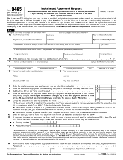


© Copyright 2026