
4-Manifolds Selman Akbulut November 7, 2014 (v.16)
4-Manifolds
(v.16)
Selman Akbulut
November 7, 2014
2
Preface
This book is an attempt to present the topology of smooth 4-manifolds in an intuitive
self contained way, as it was developed over the years. I tried to refrain long winded
pedagogic explanations, instead favoring concise direct approach to key constructions
and theorems, and then supplementing them with exercises to help reader fill in the
details which are not covered in the proofs. In short, I tried to present the material
direct way I learnt and thought to myself over the years. When there was a chance to
explain some idea with pictures I always went with pictures staying true to the saying “A
picture is worth a thousand words”. Clearly the material covered in this book is biased
towards my interest. I tried to ordered the material in historical order when possible,
while avoiding to be encyclopedic complete referencing when discussing various results.
For the sake of simplicity, I made no attempts to cover all the related results around
the materials discussed, and later I picked various examples to show how to analyze
them with the techniques developed in the earlier chapters. I want to thank many of
the friends and the collaborators R. Kirby, C. Taubes, R. Matveyev, Y. Eliashberg, R.
Fintushel, B. Ozbagci, A. Akhmedov, S. Durusoy, C. Karakurt, F. Arikan, and K. Yasui
who helped me understand this rich filed of 4-manifolds as well as patiently tutoring me
in the related fields of symplectic topology and gauge theory over the years.
i
0 Preface
ii
Contents
Preface
1 4-manifold handlebodies
1.1 Carving . . . . . . . . .
1.2 Sliding handles . . . . .
1.3 Canceling handles . . .
1.4 Carving ribbons . . . .
1.5 Non-orientable handles
i
.
.
.
.
.
.
.
.
.
.
.
.
.
.
.
.
.
.
.
.
.
.
.
.
.
.
.
.
.
.
.
.
.
.
.
.
.
.
.
.
.
.
.
.
.
.
.
.
.
.
.
.
.
.
.
.
.
.
.
.
.
.
.
.
.
.
.
.
.
.
.
.
.
.
.
.
.
.
.
.
.
.
.
.
.
.
.
.
.
.
.
.
.
.
.
.
.
.
.
.
5
8
10
12
14
18
2 Building low dimensional manifolds
2.1 Plumbing . . . . . . . . . . . . . . . . . . .
2.2 Self plumbing . . . . . . . . . . . . . . . . .
2.3 Some useful diffeomorphisms . . . . . . . .
2.4 Algebraic topology . . . . . . . . . . . . . .
2.5 Examples . . . . . . . . . . . . . . . . . . .
2.6 Constructing diffeomorphisms by carving
2.7 Shake slice knots . . . . . . . . . . . . . . .
.
.
.
.
.
.
.
.
.
.
.
.
.
.
.
.
.
.
.
.
.
.
.
.
.
.
.
.
.
.
.
.
.
.
.
.
.
.
.
.
.
.
.
.
.
.
.
.
.
.
.
.
.
.
.
.
.
.
.
.
.
.
.
.
.
.
.
.
.
.
.
.
.
.
.
.
.
.
.
.
.
.
.
.
.
.
.
.
.
.
.
.
.
.
.
.
.
.
.
.
.
.
.
.
.
.
.
.
.
.
.
.
.
.
.
.
.
.
.
.
.
.
.
.
.
.
.
.
.
.
.
.
.
21
23
24
25
26
27
31
34
3 Gluing 4 manifolds along their boundaries
3.1 Constructing −M ⌣f N by upside down method . . . . . . . . . . . . . . .
3.2 Constructing −M ⌣f N and M(f ) by cylinder method (ropes) . . . . . . .
3.3 Codimension zero surgery M ↦ M ′ . . . . . . . . . . . . . . . . . . . . . . .
35
35
37
40
4 Bundles
4.1 T4 = T 2 × T 2 . . . . . . . . . . . . . .
4.2 Cacime surface . . . . . . . . . . . . .
4.3 General surface bundles over surfaces
4.4 Circle bundles over 3-manifolds . . .
41
41
43
50
50
.
.
.
.
.
.
.
.
.
.
.
.
.
.
.
.
.
.
.
.
.
.
.
.
.
.
.
.
.
.
.
.
.
.
.
1
.
.
.
.
.
.
.
.
.
.
.
.
.
.
.
.
.
.
.
.
.
.
.
.
.
.
.
.
.
.
.
.
.
.
.
.
.
.
.
.
.
.
.
.
.
.
.
.
.
.
.
.
.
.
.
.
.
.
.
.
.
.
.
.
.
.
.
.
.
.
.
.
.
.
.
.
.
.
.
.
.
.
.
.
.
.
.
.
.
.
.
.
.
.
.
.
.
.
.
.
.
.
.
Contents
4.5
3-manifold bundles over the circle . . . . . . . . . . . . . . . . . . . . . . . .
5 3-manifolds
5.1 Dehn surgery . . . . . . . . . . . . . . . .
5.2 From framed links to Heegard diagrams
5.3 Gluing knot complements . . . . . . . . .
5.4 Carving 3-manifolds . . . . . . . . . . . .
5.5 Rohlin invariant . . . . . . . . . . . . . .
51
.
.
.
.
.
53
54
55
57
59
60
.
.
.
.
.
.
61
61
64
65
66
68
71
.
.
.
.
.
73
75
76
79
82
87
.
.
.
.
.
.
.
91
92
94
95
97
99
100
101
9 Exotic 4-manifolds
9.1 Constructing small exotic manifolds . . . . . . . . . . . . . . . . . . . . . .
9.2 Iterated 0-Whitehead doubles are non-slice . . . . . . . . . . . . . . . . . .
9.3 An exotic non-orientable closed manifold . . . . . . . . . . . . . . . . . . .
103
103
105
108
6 Operations
6.1 Gluck twisting . . . . . .
6.2 Blowing down ribbons . .
6.3 Logarithmic transform . .
6.3.1 Luttinger surgery
6.4 Knot surgery . . . . . . .
6.5 Rational blowdowns . . .
7 Lefschetz Fibrations
7.1 E(n) . . . . . . . .
7.2 Dolgachev surfaces
7.3 PALFs . . . . . . .
7.4 ALFs . . . . . . .
7.5 BLFs . . . . . . .
. .
.
. .
. .
. .
.
.
.
.
.
.
.
.
.
.
.
.
.
.
.
.
.
.
.
.
.
.
.
.
.
.
.
.
.
.
.
.
.
.
.
.
.
.
.
.
.
.
.
.
.
.
.
.
.
.
.
.
.
.
.
.
.
.
.
.
.
.
.
.
.
.
.
.
.
.
.
.
.
.
.
.
.
.
.
.
.
.
.
.
.
.
.
.
.
.
.
.
.
.
.
.
.
.
.
.
.
.
.
.
.
.
.
.
.
.
.
.
.
.
.
.
.
.
.
.
.
.
.
.
.
8 Symplectic Manifolds
8.1 Contact Manifolds . . . . . . . . . . . . . .
8.2 Stein Manifolds . . . . . . . . . . . . . . . .
8.3 Eliashberg’s characterization of Stein . . .
8.4 Convex decomposition of 4-manifolds . . .
8.5 M 4 = ∣BLF ∣ . . . . . . . . . . . . . . . . . .
8.6 Stein = ∣P ALF ∣ . . . . . . . . . . . . . . .
8.7 Imbedding Stein to Symplectic via PALF
2
.
.
.
.
.
.
.
.
.
.
.
.
.
.
.
.
.
.
.
.
.
.
.
.
.
.
.
.
.
.
.
.
.
.
.
.
.
.
.
.
.
.
.
.
.
.
.
.
.
.
.
.
.
.
.
.
.
.
.
.
.
.
.
.
.
.
.
.
.
.
.
.
.
.
.
.
.
.
.
.
.
.
.
.
.
.
.
.
.
.
.
.
.
.
.
.
.
.
.
.
.
.
.
.
.
.
.
.
.
.
.
.
.
.
.
.
.
.
.
.
.
.
.
.
.
.
.
.
.
.
.
.
.
.
.
.
.
.
.
.
.
.
.
.
.
.
.
.
.
.
.
.
.
.
.
.
.
.
.
.
.
.
.
.
.
.
.
.
.
.
.
.
.
.
.
.
.
.
.
.
.
.
.
.
.
.
.
.
.
.
.
.
.
.
.
.
.
.
.
.
.
.
.
.
.
.
.
.
.
.
.
.
.
.
.
.
.
.
.
.
.
.
.
.
.
.
.
.
.
.
.
.
.
.
.
.
.
.
.
.
.
.
.
.
.
.
.
.
.
.
.
.
.
.
.
.
.
.
.
.
.
.
.
.
.
.
.
.
.
.
.
.
.
.
.
.
.
.
.
.
.
.
.
.
.
.
.
.
.
.
.
.
.
.
.
.
.
.
.
.
.
.
.
.
.
.
.
.
.
.
.
.
.
.
.
.
.
.
.
.
.
.
.
.
.
.
.
.
.
.
.
.
.
.
.
.
.
.
.
.
.
.
.
.
.
.
.
.
.
.
.
.
.
.
.
.
.
.
.
.
.
.
.
.
.
.
.
.
.
.
.
.
.
.
.
.
.
.
.
.
.
.
.
.
.
.
.
.
.
.
.
.
.
.
.
.
.
.
.
.
.
.
.
.
.
.
.
.
.
.
.
.
.
.
Contents
10 Cork decomposition
10.1 Corks . . . . . . . .
10.2 Anticorks . . . . .
10.3 Knotting corks . .
10.4 Plugs . . . . . . . .
.
.
.
.
111
113
117
119
120
11 Covering spaces
11.1 Handlebody of coverings . . . . . . . . . . . . . . . . . . . . . . . . . . . . .
11.2 Handlebody of branched coverings . . . . . . . . . . . . . . . . . . . . . . .
11.3 Branched covers along ribbon surfaces . . . . . . . . . . . . . . . . . . . . .
125
125
127
133
12 Complex surfaces
12.1 Milnor fibers of isolated singularities . . .
12.2 Hypersurfaces that are branched covers of
12.2.1 Handlebody descriptions of Vd . .
12.3 Σ(a, b, c) . . . . . . . . . . . . . . . . . . . .
.
.
.
.
135
135
138
140
143
.
.
.
.
.
.
.
.
.
147
148
150
155
157
158
164
165
172
173
.
.
.
.
.
.
177
177
181
183
190
190
201
.
.
.
.
.
.
.
.
.
.
.
.
.
.
.
.
.
.
.
.
.
.
.
.
.
.
.
.
.
.
.
.
.
.
.
.
.
.
.
.
.
.
.
.
.
.
.
.
.
.
.
.
.
.
.
.
.
.
.
.
.
.
.
.
. . .
CP2
. . .
. . .
13 Seiberg-Witten invariants
13.1 Representations . . . . . . . . . . . . . . . . . .
13.2 Action of Λ∗ (X) on W ± . . . . . . . . . . .
13.3 Dirac Operator . . . . . . . . . . . . . . . . . .
13.4 A Special Calculation . . . . . . . . . . . . . .
13.5 Seiberg-Witten invariants . . . . . . . . . . . .
13.5.1 Seiberg-Witten for X with b+2 (X) = 1
13.6 Almost Complex and Symplectic Structures .
13.7 Seiberg-Witten equations on R × Y 3 . . . . .
13.8 Adjunction inequality . . . . . . . . . . . . . .
14 Some applications
14.1 10/8 Theorem . . . . . . . . . . . . . .
14.2 Antiholomorphic quotients . . . . . .
14.3 Cappell-Shaneson homotopy spheres
14.4 Some small closed exotic manifolds .
¯ 2 . . . . .
14.4.1 An exotic CP2 #3CP
¯ 2 . . . . .
14.4.2 An exotic CP2 #2CP
.
.
.
.
.
.
.
.
.
.
.
.
.
.
.
.
.
.
.
.
.
.
.
.
.
.
.
.
.
.
.
.
.
.
.
.
.
.
.
.
.
.
.
.
.
.
.
.
.
.
.
.
.
.
.
.
.
.
.
.
.
.
.
.
.
.
.
.
.
.
.
.
.
.
.
.
.
.
.
.
.
.
.
.
.
.
.
.
.
.
.
.
.
.
.
.
.
.
.
.
.
.
.
.
.
.
.
.
.
.
.
.
.
.
.
.
.
.
.
.
.
.
.
.
.
.
.
.
.
.
.
.
.
.
.
.
.
.
.
.
.
.
.
.
.
.
.
.
.
.
.
.
.
.
.
.
.
.
.
.
.
.
.
.
.
.
.
.
.
.
.
.
.
.
.
.
.
.
.
.
.
.
.
.
.
.
.
.
.
.
.
.
.
.
.
.
.
.
.
.
.
.
.
.
.
.
.
.
.
.
.
.
.
.
.
.
.
.
.
.
.
.
.
.
.
.
.
.
.
.
.
.
.
.
.
.
.
.
.
.
.
.
.
.
.
.
.
.
.
.
.
.
.
.
.
.
.
.
.
.
.
.
.
.
.
.
.
.
.
.
.
.
.
.
.
.
.
.
.
.
.
.
.
.
.
.
.
.
.
.
.
.
.
.
.
.
.
.
.
.
.
.
.
.
.
.
.
.
.
.
.
.
.
.
.
.
.
.
.
.
.
.
.
.
.
.
.
.
.
.
.
.
.
.
.
.
.
.
.
.
.
.
.
.
.
.
.
.
.
.
.
.
.
.
.
.
.
.
.
.
.
.
.
.
.
.
.
.
.
.
.
.
.
.
.
.
.
.
.
.
.
.
.
.
.
.
.
.
.
.
.
.
.
.
3
Contents
4
Chapter 1
4-manifold handlebodies
Let M m and N m be smooth manifolds. We say M m is obtained from N m by attaching a
k-handle and denote M = N ⌣ϕ hk , if there is an imbedding ϕ ∶ S k−1 × B m−k ↪ ∂N, such
that M is obtained from the disjoint union N and B k × B m−k by identification
M m = [N ⊔ B k × B m−k ]/ϕ(x) ∼ x
(and the corners smoothed)
Here ϕ(S k−1 × 0) is called the attaching sphere, and 0 × S m−k−1 is called the belt sphere of
this handle. We say ∂M is obtained from ∂N by surgering the k − 1 sphere ϕ(S k−1 × 0).
There is always a Morse function f ∶ M → R on M inducing a handle decomposition
M = ∪m
k=0 Mk , with φ = M−1 ⊂ M0 ⊂ .. ⊂ Mm = M, and Mk is obtained from Mk−1
by attaching k-handles [M1]. This is called a handlebody structure of M. If M m is
compact and connected we can assume that it has one 0-handle and one m-handle. So
in particular in the case of dimension four, M 4 is obtained from B 4 (the zero handle) by
attaching 1, 2, and 3-handles and then capping it off with B 4 at the top (the 4-handle).
In [S] Smale, and also independently in [W] Wallace, defined and studied handlebody structures on smooth manifolds. Smale went further by turning the operations on
handlebody structures into a great technical machine to solve difficult problems about
smooth manifolds, such as the smooth h-cobordism theorem which implied the proof of
the topological Poincare conjecture in dimensions ≥ 5. The two basic techniques which
he utilized were the handle sliding operation and handle canceling operation [H].
Given a smooth connected 4-manifold M 4 , by using its handlebody we can basically
see the whole manifold as follows: As shown in Figure 1.1 we place ourselves on the
boundary S 3 of its 0-handle B 4 and watch the feet (the attaching regions) of the 1- and
2- handles. The feet of the 1-handles will look like the pair of balls of same color, and
the feet of 2-handles will look like imbedded framed circles (framed knots) which might
go over the 1-handles. This is because the 2-handles are attached after the 1-handles.
5
1 4-manifold handlebodies
2-handles
1-handle
B
4
3-handles
2-handles
S
1-handles
3
4
B
4
B
M
4
Figure 1.1: Handlebody of a 4-manifold
Fortunately we don’t need to visualize the attaching S 2 ’s of the 3-handles, because
of an amazing theorem of Laudenbach and Poenaru [LP], which says that connected
smooth 4-manifolds are determined by their 1- and 2-handles (i.e. if there are 3-handles
they are attached uniquely!)
The feet of a 1-handle in S 3 will appear as a pair of balls B 3 , where on the boundary they are identified by the map (x, y, z) ↦ (x, −y, z) (with respect to the standard
coordinate axis placed at their origins)
z
z
y
-y
x
x
Figure 1.2
Any 2-handle which does not go over the 1-handles is attached by an imbedding
ϕ ∶ S 1 × B 2 → R3 ⊂ S 3 , which we call a framing. This imbedding is determined by the
knot K = ϕ(S 1 × (0, 0)), together with an orthonormal framing e = {u, v} of its normal
bundle in R3 . This framing e determines the imbedding ϕ by
ϕ(x, λ, ν) = (x, λu + νv)
6
Also note that by orienting K and using the right hand rule, one normal vector field u
determines the other normal vector v. Hence any normal vector field of K determines
a framing, which is parametrized by π1 (SO2 ) = Z. We make the convention that the
normal vector field induced from the collar of any Seifert surface of K to be the zero
framing u0 (check this is well defined, because linking number is well defined). Once
this is done, it is clear that any k ∈ Z corresponds to the vector field uk which deviates
from u0 by k-full twist. Put another way, uk is the vector field when we push K along
it, we get a copy of K which has linking number k with K. So we denote framings by
integers. The following exercise gives a useful tool of deciding the k-framing.
Exercise 1.1. Orient a diagram of the knot K, and let C(K) be the set of its crossing
points, define writhe w(K) of a knot K to be the integer
w(K) = ∑ ǫ(p)
p∈C(K)
where ǫ(p) is +1 or −1 according to right or left handed crossing at p. Show that the
blackboard framing (parallel on the surface of the paper) of a knot equals to its writhe
u0
K
Figure 1.3: w(K) = 3 and u0 is the zero framing
When the attaching framed circles of 2-handles go over 1-handles their framing can
not be a well defined integer. For example, by the isotopy of Figure 1.4 the framing
can be changed by adding or subtracting 2. One way to prevent this framing changing
isotopy is to fix an arc, as shown in Figure 1.2, connecting the attaching balls of the
1-handle, and make the rule that no isotopy of framed knots may cross this arc. Only
after this unnatural rule, we can talk about well defined framed circles. Most of the
work of [AK1] is based on this convention.
7
1 4-manifold handlebodies
Figure 1.4
1.1
Carving (invariant notation of 1-handle)
Carving is based on the following simple observation: If the attaching sphere ϕ(S k−1 ×0)
of the k-handle of M = N m ⌣ϕ hk , bounds a disk in ∂N, then M can be obtained
from N by excising (drilling) out an open tubular neighborhood of a properly imbedded
disk D m−k−1 ⊂ N. This is because we can cancel the k-handle by the obvious (k + 1)handle and get back N (Section 1.3), then we can undo the (k +1)-handle by puncturing
(carving) it, as indicated in Figure 1.5. In particular if M 4 is connected, attaching a
1-handle to M 4 is equivalent to carving out a properly imbedded 2-disk D 2 ⊂ B 4 from
the 0-handle B 4 ⊂ M. This simple observation has many useful consequences (e.g. [A1]).
2
2
B
1-handle
1
B
3
B
N + (1-handle)
x
D
2
0 x D removed
N
drill
cancel
=
N-D
Figure 1.5: Attaching 1-handle is the same as drilling 2-disk
To distinguish the boundary of the carved disk ∂D ⊂ S 3 from the attaching cirlces
of the 2-handles, we will put a “dot” on that circle. In particular this means a path
going through this dotted circle is going over the associated 1-handle. So the observer
in Figure 1.1 standing on the boundary of B 4 will see the 4-manifold as in Figure 1.6.
As discussed before, the framing of the attaching circle of each 2-handle is specified by
an integer, so the knots come with integers (in this example the framings are 2 and 3).
8
1.1 Carving
This notation of 1-handle has the advantage of not creating ambiguity on the framings
of framed knots going through it, as it happens in Figure 1.4. Also this notation can
be helpful in constructing hard to see diffeomorphisms between the boundaries of 4manifolds (e.g. Exercise 1.3, Section 2.6).
3
2
Figure 1.6
We will denote an r-framed knot K by K r , which will also denote the corresponding
4-manifold (B 4 plus 2-handle). Since any smooth 4-manifold M 4 is determined by its 0,
1 and 2-handles, M can be denoted by a link of framed knots K1r1 , K2r2 , .. (2-handles),
along with “circle with dots” C1 , C2 , .. (1-handles). Note that we have the option of
denoting the 1-handles either by dotted circles, or pair of balls (each notation has its
own advantages). Also for convenience, we will orient the components of this link:
Λ = {K1r1 , .., Knrn , C1 , .., Cs }
We notate the corresponding 4-manifold by M = MΛ . For example, Figure 1.6 is the
4-manifold MΛ with Λ = {K12 , K23 , C}, where K1 is the trefoil knot, and K2 is the circle
which links K1 , and C is the 1-handle. Notice that a 0-framed unknot denotes S 2 × B 2 ,
it also denotes S 4 if we state that there is a 3-handle is present. Also a ±1-framed unknot
denotes a punctured (that is a 4-ball removed) ±CP2
Exercise 1.2. Show that S 1 × B 3 and B 2 × S 2 are related to each other by surgeries of
their core spheres (i.e. the zero and dot exchanges in Figure 1.7)
surgery to S
S
2
xB
2
=
2
0
=
surgery to S
1
S xB
3
1
Figure 1.7
9
1 4-manifold handlebodies
Exercise 1.3. Show that the manifold W in Figure 1.8 is a contractible manifold, and
surgeries in its interior (corresponding to zero and dot exchanges on the symmetric link)
gives an involution on its boundary f ∶ ∂W → ∂W , where the indicated loops a, b are
mapped to each other by the involution f .
b
a
a
0
b
b
f
0
W
W
0
a
=
W
Figure 1.8
1.2
Sliding handles
As explained in [S], [H] we can change a given handlebody of M to another handlebody
of M, by sliding any k-handle over another r-handles with r ≤ k.
Figure 1.9: Sliding a 2-handle over another 2-handle
In particular in a 4-manifold we can perform the following handle sliding operations:
We can (a) slide a 1-handle over another 1-handle, or (b) slide a 2-handle over a 1-handle
or (c) slide a 2-handle over another 2- handle. This process alters the framings of the
attaching circles of the 2-handles in a well defined way as follows.
10
1.2 Sliding handles
Exercise 1.4. Let Λ = {K1r1 , .., Knrn , C1 , .., Cs } be an oriented framed link with circle with
dots, let µij be the linking number of Ki and Cj , and λij be the linking number of Ki
and Kj . Also let Ki′ denote a parallel copy of Ki (Ki pushed off by the framing ri ), and
Ci′ be a parallel copy of the circle Ci . Show that the handle slides (a), (b), (c) above
corresponds to changing one of the elements of Λ as indicated below (j ≠ s):
(a) Ci ↦ Ci + Cj′ ∶= The circle obtained, by connected summing Ci to Cj′ along any arch
which does not go through any of the Ck′ ’s.
¯ r¯i The framed knot obtained, by connected summing Ki to Cs′
(b) Kiri ↦ Ki + Cj′ ∶= K
i
along any arc, with framing r¯i = ri + 2µij
¯ r¯i The framed knot obtianed, by connected summing Ki to K ′
(c) Kiri ↦ Ki + Kj′ ∶= K
j
i
along any arc, with framing r¯i = ri + rj + 2λij
These rules are best explained by the following examples:
(a)
(b)
3
2
1
2
(c)
0
1
0
-1
Figure 1.10: Examples of handle slides (a), (b), (c)
11
1 4-manifold handlebodies
1.3
Canceling handles
We can cancel a k-handle hk with a (k + 1)-handle hk+1 provided that the attaching
sphere of hk+1 meets the belt sphere of hk transversally at a single point (as explained
in [S] and [H]). This means that we have a diffeomorphism:
N ⌣ϕ hk ⌣ψ hk+1 ≈ N
For example, in Figure 1.5 a canceling 1 and 2-handle pairs, of a 3-manifold, was drawn.
Any 1-handle, and a 2-handle whose attaching circle (framed knot) goes through the
1-handle geometrically once, forms is a canceling pair. If no other framed knot goes
through the 1-handle of the canceling pair, simply erasing the pair from the picture
corresponds to canceling operation. Figure 1.11 gives three equivalent descriptions of a
canceling handle pair, so if you want to cancel just erase them from the picture.
-2
-2
=
-2
=
Figure 1.11
It follows from the handle sliding description that, if there are other framed knots
going through the 1-handle of a canceling handle pair, the extra framed knots must
be slid over over the 2-handle of the canceling pair, before the canceling operation is
performed (erasing the pair from the picture)
-2
cancel
slide
...
=
...
...
...
Figure 1.12
Notice that since 3-handles are attached uniquely, introducing a canceling 2- and 3handle pair is much simpler operation. We just draw the 2-handle as 0-framed unknot,
12
1.3 Canceling handles
which is S 2 × B 2 , and then state that there is a canceling 3-handle on top of it. In a
handle picture of 4-manifold, no other handles should go through this 0-framed unknot
to be able to cancel it with a 3-handle.
Exercise 1.5. Verify the diffeomorphisms of Figure 1.13 by handle slides (the integers
±1 across the stands indicate ±1 full twist). Also show that this operation changes the
framing of any framed knot, which links the ±1 framed unknot r times, by r 2 .
1
-1
-1
-1
1
1
slide
slide
Figure 1.13
¯ 2 are diffemorphic to each
Exercise 1.6. Show that S 2 × S 2 #CP2 and CP2 #CP2 #CP
other by sliding operations as shown in Figure 1.14 (the identification of these two 4manifolds is originally due to Hirzebruch).
0
0
0
-1
-1
slide
=
1
-1
0
slide
1
-1
0
-1
slide
Figure 1.14
The operation M ↦ M# ± CP2 is called blowing up operation, and its converse is
called blowing down operation. If C ±1 is an unknot with ±1 framing in a framed link
Λ, then by the handle sliding operations of Exercise 1.5, we obtain a new framed link
Λ′ containing C ±1 such that C ±1 does not link any other components of Λ′ . So we can
write Λ′ = Λ′′ ⊔ {C ±1 }. Therefore we have the identification MΛ = MΛ′′ #(±CP2 ), and
hence a diffeomorphism of 3-manifolds ∂MΛ ≈ ∂MΛ′′ . Sometimes the operations Λ ↔ Λ′′
on framed links are called blowing up/down operations (of the framed links).
13
1 4-manifold handlebodies
-1
-1
1
1
Figure 1.15: Blowing up/down operation
Recall that the set Λ of framed links encodes handle information on the corresponding
4-manifold M = MΛ , which comes from a Morse function f ∶ M → R. Cerf theory studies
how two different Morse function on a manifold are related to each other [C]. In [K1],
by using Cerf theory, Kirby studied the map Φ defined by Λ ↦ ∂MΛ , from framed links
to 3-manifolds. It is known that Φ is onto [Li] (see Chapter 5).
Φ ∶ {Framed links} ↦ {closed oriented 3 − manifolds}
In [K1] it was shown that under Φ any two framed links are mapped to the same 3manifold if and only if they are related to each other by handle sliding operation of
Exercise 1.4 (c), and blowing up or down operations. For this reason, in literature
manipulating framed links by these two operations is usually called Kirby calculus.
1.4
Carving ribbons
In some cases carving operation allows us to slide a 1-handles over a 2-handles, which
is in general prohibited (the attaching circle of the 2-handle might go through the 1handle). But as in the configuration of Figure 1.16, we can imagine the carved disk
(painted yellow inside) as a trough (or a groove) just below the surface; then sliding it
over the 2-handle (imagine as a surface of a helmet) by indicated isotopy makes sense.
k
slide
k
Figure 1.16
14
k
1.4 Carving ribbons
Exercise 1.7. Justify the isotopy of Figure 1.16, by first breaking the 1-handle into a
1-handle and a canceling 1 and 2-handle pair, as in the first picture of Figure 1.17, then
by sliding the new 2-handle over the 2-handle of Figure 1.16, then at the end by canceling
back the 1 and 2-handle pair. Also verify the second picture of Figure 1.17.
0
...
0
...
cancel
...
0
cancel
...
...
...
...
0
...
Figure 1.17
This move can turn a 1-handle, which is a carved disk in B 4 bounding an unknot (in
a nonstandard handlebody of B 4 ) into a carved ribbon disk bounding a ribbon knot (in
the standard handlebody of B 4 ), as in the example of Figure 1.18.
0
0
isotopy
cancel
slide
-1
0
Figure 1.18
We can also consider this operation in the reverse, namely given a ribbon knot, how
can we describe complement of the slice disk which ribbon knot bounds in B 4 ? i.e.
what is the ribbon complement obtained by carving this ribbon disk from B 4 ? Clearly
by ribbon moves (i.e. cutting and regluing along bands) we can turn the ribbon knot
into disjoint union of unknotted circles, which we can use to carve B 4 along the disks
they bound, getting some number of connected sum #k (S 1 × B 3 ). Now we can do the
reverse of the ribbon moves, which describes a cobordism from the boundary #k (S 1 ×S 2 )
of the carved B 4 to the ribbon complement in S 3 . During this cobordism every time
two circles coalesce the complement gains a 2-handle as in Figure 1.19. To sum up, to
construct the complement of the ribbon which K bounds in B 4 , we perform k ribbon
moves (for some k) turning K into k disjoint unknots {Cj }kj=1, and after every ribbon
move we add a 2 handle as indicated in Figure 1.19, and put dots on the circles {Cj }kj=1.
15
1 4-manifold handlebodies
...
ribbon
move
...
...
reverse
ribbon
move
carved disjoint circles
ribbon knot
0
...
=
carved ribbon knot
Figure 1.19
For example, applying this process to the ribbon knot K of Figure 1.20 gives the
handlebody at the bottom right picture of Figure 1.20 (this knot appears in [A2] playing
important role in exotic smooth structures of 4-manifolds). Note that this process turns
carving a ribbon from the standard handlebody picture of B 4 into carving the trivial
disks from an non standard handlebody picture of B 4 . Clearly the top left picture is
the handlebody of the complement of an imbedding S 2 ↪ S 4 obtained by doubling this
ribbon complement in B 4 as in Figure 1.21 (we build this handlebody from the bottom
#2 (S 1 × B 3 ) to top by attaching 2-handles corresponding to the reverse ribbon moves).
0
reverse
ribbon
move
K
0
ribbon move
along the
dotted line
0
K
reverse
ribbon
move
Figure 1.20
16
1.4 Carving ribbons
K
Figure 1.21
Exercise 1.8. Show that the indicated ribbon move to the ribbon knot of Figure 1.22 gives
the ribbon complement in B 4 (the second picture), which consisting of two 1-handles and
one 2-handle, and the third picture (with an extra 2-handle and an invisible 3-handle)
is the complement of the double of this ribbon disk (i.e. a copy of S 2 ) in S 4 . Also by
handle slides verify the last diffeomorphism.
0
0
0
K
ribbon
move
K
0
0
double
K
K
Figure 1.22
So in general, imbeddings S 2 ⊂ S 4 obtained by doubling ribbons look like Figure 1.23,
which is consistent with the doubling process discussed in Section 3.1.
0
K
0
0
Figure 1.23: Complement of the double of a ribbon S 2 ⊂ S 4
17
1 4-manifold handlebodies
1.5
Non-orientable handles
3
If we attach a 1-handle B 1 × B 3 to B 4 along a pair of balls {B−3 , B+∣
} with the same
4
orientation of ∂B we get a orientation reversing 1-handle, which is the nonoriented B 3 bundle over S 1 . So to an observer, located at the boundary of B 4 , this will be seen as a
pair of balls with their interiors identified by the map (x, y, z) ↦ (x, −y, −z). To denote
this in pictures, we use the notation adapted in [A3], by drawing a pair of balls with
little arcs passing through their centers, which means that the usual oriented 1-handle
identification is augmented by reflection across the plane which is orthogonal to these
arcs (Figure 1.24). When drawing the frame knots going through these handles, one
z
=
-y
y
x
x
-z
Figure 1.24
should not forget which points of the spheres ∂B−3 and ∂B+3 correspond to each other
via the 1-handle. Also framings of the framed knots going through these handles are
not well defined, not just because of the isotopies of Figure 1.4, but also going through
an orientation reversing handle the framing changes sign. For that reason when these
handles are present, we will conservatively mark the framings by circled integers (with
the knowledge that pushing them through the handle that integer changes its sign). For
the same reason, any small knot tied to a strand going through this handle will appear
as its mirror image when its is pushed though this handle, as indicated in Figure 1.25.
push
=
-m
m
Figure 1.25
Sometimes to simplify the handlebody picture, we place one foot of a orientation
reversing 1- handle at the point of infinity ∞ (continue traveling west to ∞ you will
appear to be coming back from the east with your orientation reversed), as in the example
of Figure 1.26. Notice that when we attach B 4 an orientation reversing 1-handle, we get
∼
the orientation reversing D 3 bundle over S 1 , denoted by D 3 × S 1 .
18
1.5 Non-orientable handles
Exercise 1.9. Show that the diffeomorphism type of the manifold M(p, q) in Figure 1.26
∼
depends only on parity of p+q, it is D 2 ×RP2 if the parity is even, or else it is D 2 × RP2 (a
∼
twisted D 2 -bundle over RP2 ). Also prove that there is the identification ∂(D 2 × RP2 ) ≈
∼
∂(D 3 × S 1 ).
p
p
=
q
q
Figure 1.26: M(p,q)
∼
Now if D 2 × RP2 ⊂ M 4 , we define Blowing down RP2 operation as:
M ↦ (M − D 2 × RP2 ) ⌣∂ (D 3 × S 1 )
∼
∼
Figure 1.27 shows how this operation is performed in a handlebody.
other
framed
knots
...
1
...
...
-1
...
...
-1
Figure 1.27: Blowing down RP2 operation
∼
By using this, in [A3], an exotic copy of S 3 × S 1 # S 2 × S 2 was constructed (the
second picture of Figure 1.28). A discussion of this manifold is given in Section 9.3.
0
0
1
Standard
Exotic
∼
Figure 1.28: Standard and exotic S 3 × S 1 # S 2 × S 2
19
1 4-manifold handlebodies
20
Chapter 2
Building low dimensional manifolds
Just as we visualized 4-manifolds by placing ourselves on the boundary of its 0-handle
(Figure 1.1) and observing the feet of 1 and 2-handles, we can visualize 2 and 3 manifolds by placing ourselves on the boundary of their 0 handles. By this way we get
analogous handlebody pictures as in Figures 2.1 and 2.2, except in this case we don’t
need to specify the framings of the attaching circles of the 2-handles. The 3-manifold
handlebody pictures obtained this way are called Heegaard diagrams. Clearly we can
thicken these handlebodie pictures by crossing them with balls to get higher dimensional
handlebodies as indicated in these figures. For example, the middle picture of Figure 2.1
is a Heegard diagram of T 2 × I and the last picture is T 2 × B 2 , and the Figure 2.2 is a
Heegaard diagram of S 3 , and a handlebody of S 3 × B 1 .
0
T
2
2
T xI
Figure 2.1
21
2
T xB
2
2 Building low dimensional manifolds
0
=
0
Y
Y
3
3
3
Y xI
Figure 2.2: Y 3 = S 3
After this, by changing the 1-handle notations to the circle with dot notation, in
Figure 2.3 we get a handlebody picture of T 2 × B 2 , and proceeding in the similarly way
we get a handlebody of Fg × B 2 , where Fg denotes the surface of genus g.
g
0
0
T2
...
F
x B2
g
x
B
2
Figure 2.3
Exercise 2.1. By using this method verify Exercise 1.9, and also show that the handlebody pictures in Figure 2.4 are twisted D 2 bundles over S 2 , RP2 , and Fg , respectively
(more specifically they are all Euler class k D 2 -bundles).
g
k
k
k
Figure 2.4
22
...
2.1 Plumbing
2.1
Plumbing
For i = 1, 2 let Di ↪ Ei → Si be two Euler class ki disk bundles over the 2-spheres Si ,
≈
and let Bi ⊂ Si be the disks giving the trivializations Ei ∣Bi → Bi × Di . Plumbing E1
and E2 is the process of gluing them together by identifying D1 × B1 with B2 × D2 (by
switching base and fiber directions). Hence, in this manifold if we locate ourselves on
the boundary of D1 × B1 = B 4 we will see a two 2-handles attached to B 4 along the link
of Hopf circles {∂D1 , ∂B1 } with framings k1 , k2 . This plumbed manifold is symbolically
denoted by a graph with one edge and two vertices weighted by integers k1 and k2 .
k2
k1
Figure 2.5
By iterating this process we can similarly construct 4-manifolds corresponding to any
graph whose verticies weighted with integers. Also in this construction Si ’s don’t have
to be spheres, they can be any surfaces (orientable or not), but in this case when we
abbreviate these plumbings by graphs, to each of its vertex we need to specify a specific
surface along side an integer weight. Reader can check that the manifolds corresponding
to the graphs in Figure 2.6 are given by the handlebodies on the right.
2
3
F
-2
5
RP
2
#
RP
3
2
T
2
=
3
3
2
=
2
-2
5
4
4
Figure 2.6
23
2 Building low dimensional manifolds
The following plumbed manifolds have special names: E8 and E10 .
E
-2
8
-2
-2
-2
-2
-2
-2
-2
-2 -2 -2 -2 -2
=
=
-2
-2
-2
E
10
-2
-2
-2
-2
-2
-2
-2
-2
-2 -2
-2
=
-2 -2 -2 -2 -2 -2 -2
=
-2
-2
Figure 2.7
An alternative way to denote a plumbing diagram of 2-spheres is to draw the dual
of the plumbing graph, where the weighted vertices are replace by weighted intersecting
arc segments, intersecting according to the graph (e.g. Figure 2.8).
-2
-3
-2
-2
-2
-2
=
-2
-3
-2
-2
Figure 2.8
2.2
Self plumbing
By a method similar to the one above, we can plumb a disk bundle D ↪ E → S to itself.
So the only difference is, when we locate ourselves on the boundary of D1 × B1 = B 4 , we
will see a link of thickened Hopf circles being identified with each other by a cylinder
(S 1 × [0, 1]) × D 2 . This is equivalent to first attaching a 1-handle to B 4 (thickened point
×[0, 1]), followed by attaching a 2-handle to the connected sum of the two circles over
the 1-handle (a tunnel). Figure 2.9 gives self-plumbings of Euler class k bundles over S 2
and over T 2 (see the “round handle” discussions in Definition 7.7 and Figure 3.10).
24
2.3 Some useful diffeomorphisms
k
k
=
self plumb
k
k
self plumb
Figure 2.9
2.3
Some useful diffeomorphisms
...
As shown in Figure 2.10, by introducing a canceling pair of 1 and 2-handles, and sliding
new 1-handle over the existing 1-handle, and then canceling the resulting 1 and 2-handle
pair, we get an interesting diffeomorphism between the first and last handlebodies of
this figure. These diffeomorphisms are used in [AK2] identifying various 3-manifolds.
...
1
-1
introduce
canceling
pair
-1
slide
1
-1
1
cancel
Figure 2.10
Exercise 2.2. Let W ± (l, k) be the contractible manifolds given in Figure 2.11 (where
the integer l denotes l-full twist between the stands). By using the above diffeomorphisms
construct the following diffeomorphisms:
• W (l, k) ≈ W (l + 1, k − 1)
• W − (l, k) ≈ −W + (−l, −k + 3)
25
2 Building low dimensional manifolds
k
-
k
+
W(l , k ) =
W( l , k) =
l
l
Figure 2.11: W (l, k)
2.4
Algebraic topology
Algebraic topolology of a 4-manifold M 4 can easily be red off from its handlebody
description. For example if M = MΛ , where Λ = {K1r1 , .., Knrn , C1 , .., Cs } and no 3-handle
present, to compute π1 (M) for each circle-with-dot Ci we introduce a generator xi , then
each loop Kj gives a relation rj (x1 , .., xs ) recording how it goes through the 1-handles.
Also homology groups of M can be computed from the cell complex given by its 1 and
2-handles. For example, to any α = ∑j cj Kj with cj ∈ Z we can associate [α] ∈ H1 (M)
(by thinking Kj as loops). Alternatively, when [α] = 0, we can view α as a CW 2-cycle
and think of α ∈ H2 (M). The intersection form (α, β) ↦ α.β on H2 (M)
qM ∶ H2 (M; Z) ⊗ H2 (M; Z) Ð→ Z
r
can be computed from these classes: For example if α = ∑i ci Kiri and β = ∑j c′j Kj j ,
then α.β = ∑i,j ci c′j L(Ki , Kj ), where L(Ki , Kj ) is the linking number of Ki and Kj . In
particular L(Kj , Kj ) is given by the framing rj of Kj . The signature of the bilinear
form qM is defined to be the signature σ(M) of M. When M is closed and simply
connected the intersection form qM determines the homotopy type of M ([Wh], [M2],
[MS]). Note that changing the orientation of the manifold MΛ corresponds changing Λ
to −Λ = {−K1−r1 , .., −Kk−rk , C1 , .., Cs }, where −K denotes the mirror image of the knot K.
So in short −Mλ = M−Λ . Also notice that in Λ replacing the dotted circles C1 , .., Cs with
0-framed unknots does not change the boundary ∂MΛ (Exercise 1.2).
Every closed 3-manifold Y 3 bounds a compact smooth 4-manifold M consisting of
0- and 2-handles (Chapter 5). When Λ = {K r } the following alternative notations will
be used interchangibly:
MΛ = B 4 (K, r) = K r
So ∂(K r ) will be the 3-manifold obtained by surgering S 3 along K with framing r. If
K ⊂ Y , then we will denote the 3-manifold obtained by surgering Y along K with framing
r by the notations Y (K, r) or Yr (K) (provided the framing r in Y is well defined).
26
2.5 Examples
2.5
Examples
Links of hypersurfece singularities provide rich class of 3-manifolds (Section 12.3), they
are obtained by intersecting hypersurfaces in C3 with isolated singularities at the origin
with a sphere Sǫ5 of small radius ǫ, centered at the origin. In particular the Brieskorn
3-manifolds are the boundaries of the following interesting 4-manifolds (Exercise 12.4)
Σ(a, b, c) ∶= {(x, y, z) ∈ C3 ∣ xa + y b + z c = 0} ∩ Sǫ5
0
1
-1
(2, 3, 5)
(2, 3, 9)
(2, 3, 7)
-1
0
0
(2, 3, 11)
(2, 7, 13)
(2, 3, 13)
-2
2
Figure 2.12
Σ(2, 3, 5) is called the Poincare homology sphere. There is a useful boundary identi≈
fication f ∶ Σ(2, 3, 5) → ∂E8 (see Fig 2.7) given by the steps of Figure 2.13
-1
3
-1
=
3
1
2
=
1
1
blow up
blow up
3
5
4
2
blow up
1
1
f
=
-1
-2
1
-2
-2
-2
-2
-2
-2
-2
-2
blow
downs
-2
-2
-1
4
2
1
-2
-2
-1
blow
ups
5
1
blow up
-2
-1
-1
3
2
1
-1
E8
Figure 2.13
27
2 Building low dimensional manifolds
Exercise 2.3. By imitating the steps of Figure 2.13 show that Σ(2, 3, 7) ≈ ∂E10 . Also
by justifying the diffeomorphisms in Figure 2.14 show that ∂E10 ≈ M 4 , where M 4 is a
manifold obtained from E8 by attaching pair of 2-handles, and M has the intersection
form of E8 # (S 2 × S 2 ).
-1
1
0
-1
-2
-1
Blow up then
blow down
0
-2
Figure 2.14
Exercise 2.4. By justifying steps of Figure 2.15 construct a closed simply connected
smooth manifold with signature −16 and the second Betti number 22 (In the figure M =
A + B means M contains each of the handlebodies A and B, and the handles of A and
B has zero algebraic linking number, in which case we can write M = A + handles =
B + handles, and M is homology equivalent to A # B).
1
-1
S
3
E8 +
1
0
E
8
+
E
0
0
-2
-2
+
10
E
Figure 2.15
28
+
8
-2
1
0
-2
2.5 Examples
Σ(2, 3, 13) bounds a contractible manifold, which can be seen by the identification
∂Σ(2, 3, 13) ≈ ∂W + (1, 0) as indicated in Figure 2.16.
1
0
0
-1
(2, 3, 13)
blow
up/down
blow
up
-2
-1
0
1
blow
down
1
surgery
2
1
-1
blow
down
twice
blow
up
Figure 2.16
Exercise 2.5. By blowing up and down operations verify the diffeomorphism of Figure 2.17 (Hint: imitate the initial steps of Figure 2.16).
-1
(2, 3, 11)
Figure 2.17
Exercise 2.6. By verifying the identifications of Figure 2.18, show that Σ(2, 3, 11)
bounds a definite manifold with intersection form E8 ⊕ (−1), and also bounds a smooth
simply connected manifold with signature −16 and the second Betti number 20.
29
2 Building low dimensional manifolds
-1
-1
-1
(2, 3, 11)
E8+
-1
0
E
8
+
E
0
0
-2
-2
+
8
E +
8
-2
-1
0
-2
Figure 2.18
Exercise 2.7. By thickening the handlebody of RP2 in two different ways get two diferent
D 2 bundles of RP2 , one is the trivial bundle with nonorientable total space, the other is
the twisted bundle with oriented total space (Figure 2.19). The second one is the normal
bundle of an imbedding RP2 ⊂ R4 .
isotopy
thicken
thicken
thicken
0
0
RP
2
Figure 2.19
30
2.6 Constructing diffeomorphisms by carving
2.6
Constructing diffeomorphisms by carving
≈
Given a diffeomorphism f ∶ ∂M → ∂N, when does f extend to a diffeomophism inside
F ∶ M → N? Some instances carving can provide a solution. One necessary condition
is that f must extend to a homotopy equivalence inside, so let us assume this as a
hypothesis. Now let us start with M = MΛ , where Λ = {K1rn , .., Knrn , C1 , .., Cs }, and let
{γ1 , .., γk } be the dual circles of the 2-handles. i.e. γj = ∂Bj , where Bj is the co-core of
r
the dual 2-handle of Kj j . Then if {f (γ1 ), .., f (γk )} is a slice link in N, that is if each
f (γj ) = ∂Dj where Dj ⊂ N are properly imbedded disjoint disks. Then we can extend f
to a diffeomorphism:
f ′ ∶ M ′ ∶= ∂Mǫ ⌣ ∪j ν(Bj ) → ∂Nǫ ⌣ ∪j ν(Dj ) ∶= N ′
where ∂Mǫ and ∂Nǫ are the collar neighborhoods of the boundaries, and ν(Bj ), ν(Dj )
are the tubular neighborhoods of the disks Bj , Dj .
B
j
f
K
r
carve
Dj
Figure 2.20
This reduces the extension problem to the problem of extending f ′ to complements
M − M ′ → N − N ′ . Notice that M − M ′ = #s (S 1 × B 3 ) and N − N ′ is a homotopy
equivalent to #s (S 1 × B 3 ). Since every self diffeomorphism #s (S 1 × S 2 ) extends to a
unique self diffeomorphism of #s (S 1 × B 3 ), the only way f ′ doesn’t extend to M − M ′ →
N − N ′ is N − N ′ is an exotic copy of #s (S 1 × B 3 ). The case of s = 0 is particularly
interesting, since the only way the last extension problem M − M ′ → N − N ′ fails is
when the 4-dimensional smooth Poincare conjecture fails (in examples usually this step
goes through). Even in the cases of single 2-handle M = K r and N = Lr extending
a diffeomorphism f ∶ ∂(K r ) → ∂(Lr ) can be difficult task without carving. Because
there are no other handles to slide over to construct a diffeomorphisms in a conventional
way! Cerf theory says that, if they are diffeomorphic there must be canceling handle
pairs, but we don’t know where they are? Carving at least gives us a way to start.
For example, Figure 2.21 describes a diffeomorphism between the boundaries of two
4-manifolds ([A1]).
≈
f ∶ ∂(K 1 ) Ð→ ∂(L1 )
31
2 Building low dimensional manifolds
0
1
-1
K
1
=
-1
blow up
=
0
f
blow up
0
1
L
0
=
1
1
1
isotop
and
surger
cancel
0
Figure 2.21
Figure 2.22 shows the dual circle γ and its image f (γ) under this diffeomorphism. By
carving along γ and f (γ) we can extend f to a diffeomorphism. To do this we put dots
on these circles (making 1-handles). Then we only have to check that the picture on the
right is B 4 . For this we slide two stands of the 2-handle over the 1-handle as indicated
in the figure, and then check that we get B 4 .
1
1
f
f(
)
Figure 2.22
32
2.6 Constructing diffeomorphisms by carving
The following is a generalization of the previous example from [A4]. We claim that
for each r ∈ Z − 0, there are of distinct knot pairs K and Lr (one is slice the others are
non-slice knots) such that for all r ≠ 0
K r ≈ Lrr
(2.1)
The previous example gives a hint of how to see this by Cerf theory, for this we introduce
and then cancel 1- and 2-handle pairs as shown in Figure 2.23.
r
K
r
r
r+1
= L
=
r
r
f
=
cancel
r
r-2
0
slide
0
Figure 2.23
Exercise 2.8 ([O], [T]). Show that in the boundaries ∂M and ∂N of the manifolds of
Figure 2.24 the loops a and b are isotopic to each other (Hint: slide them over the 2handle). From this produce distinct knots Kr and Lr with Kr0 ≈ Ks0 and L4r ≈ L4s for all
r ≠ s (Hint: consider repeated ±1 surgeries to a and b).
b
b
M =
a
0
a
N =
-1
0
Figure 2.24
33
2 Building low dimensional manifolds
2.7
Shake slice knots
Definition 2.1. We call a knot K r-shake slice if the link L = {K, K+ , .., K+ , K− , .., K− }
consisting of K and an even number of oppositely oriented parallel copies of K (pushed
off by the framing r) bounds disk with holes. We call L an r-shaking of the knot K.
As in the (2.1) examples, if K is a knot and L is a slice knot, such that the 4-manifods
and K r are diffeomorphic, then K is an r-shake slice. This is because L being slice
there is a smooth 2-sphere S ⊂ Lr representing the generator of the homology group
H2 (Lr ) ≅ Z (namely the slice disk which L bounds in B 4 together with the core of the
handle), then if F ∶ Lr → K r is a diffeomorphism, by making F transversal to the cocore
of the 2-handle of K r and by an isotopy, we can make the link F (S) ∩ S 3 an r-shaking
of the knot K, clearly this link bounds disk with holes (Figure 2.25). Theorem 9.4 gives
an example of pair of knots K1 and K2 , such that one is slice the other is not, and K1−1
is homeomorphic to K2−1 , even though they are not diffeomorphic to each other. So not
all knots are shake slice.
Lr
cocore
S
F
F(S)
Lr
K
r
Figure 2.25
Exercise 2.9. Tristram inequality ([Tr]) states that if an oriented link L bounds a disk
with holes in B 4 , then for any prime p:
∣σp (L)∣ + np (L) ≤ µ(L)
where σp (L), np (L) and µ(L) denote p-signature, p-nullity, and the number of components of the link L. Prove that if ∣σp (K)∣ ≥ 2 and p divides r, then K is not r-shake
slice (Hint: show that r-shaking doesn’t change the p-signature, whereas it increases the
nullity by 2m where m is the number of pairs of oppositely oriented copies to K, [A1]).
34
Chapter 3
Gluing 4 manifolds along their
boundaries
Given two connected smooth 4-manifolds with boundary M, N, and an orientation
preserving diffeomorphism f ∶ ∂M → ∂N, we can ask how to draw a handlebody of the
oriented manifold obtained by gluing with this map:
−M ⌣f N
Also we can ask when given two disjoint copies of codimension zero submanifolds L⊔−L ⊂
∂M, how can we draw the manifold M(f ) obtained from M by identifying these two
copies by a diffemorphism f ∶ L → L?
M(f ) = M ⊔ (L × [0, 1]) /
(x, 0) ∼ x ∈ L
(f (x), 1) ∼ x ∈ −L
There are two ways of doing this: The upsidedown method, and the cylinder method.
3.1
Constructing −M ⌣f N by upside down method
Let M = MΛ with Λ = {K1r1 , .., Knrn , C1 , .., Cs } and N = NΛ′ . Let {γ1 , .., γn } be the
dual zero-framed circles of the 2-handles K1 , .., Kn . Then −M ⌣f N is represented
by QΛ′′ where Λ′′ = Λ′ ⌣ {f (γ1 ), .., f (γn )}. In particular, if we apply this process to
M 0 ∶= M − {3 and 4-handles} and any diffeomorphism f ∶ ∂(M 0 ) → ∂#p (S 1 × B 3 ) (p is
the number of 3-handles), we get the upsidedown handlebody of M. In the special case
of when M has no 3-handles, then clearly the framed link {f (γ1 ), .., f (γn )} in ∂B 4 gives
its upside down handlebody of M.
35
3 Gluing 4 manifolds along their boundaries
4
B
B
4
3-handles
3-handles
M
4
2-handles
=
2-handles
-M
=
f
1-handles
4
#p
B
f(
3
B)
1
(S x
4
)
1-handles
B
4
Figure 3.1
The manifold −M ⌣id M is called the double of M and denoted by D(M). For
example, from the above description we can construct handlebody for D(T 2 × B 2 ) =
T 2 × S 2 . The Cusp is defined to be the 4-manifold K 0 , where K is the right handed
trefoil knot. By using this method, we can easily check that the double D(C) of the
cusp C is diffeomorphic to S 2 × S 2 (see Figure 3.2).
0
0
0
0
0
0
double
double
2
T xB
2
2
T xS
2
C = Cusp
2
S xS
2
Figure 3.2
Exercise 3.1. The Fishtail is defined to be the manifold of the first picture of Figure 3.3.
Let f ∶ ∂F → ∂F be the diffeomorphism on the boundary of the Fishtail described in
Figure 3.3 (obtained by the dot and 0 exchange). Show that −F ⌣f F = S 4 (given by a
canceling pair of 2 and 3-handles).
36
3.2 Constructing −M ⌣f N and M(f ) by cylinder method (ropes)
0
0
0
0
f
F = Fishtail
-F
F
f
F
=
S
4
Figure 3.3
Exercise 3.2. Let M be B 4 with a 2-handle attached to the left handed trefoil knot with
−1 framing, and f ∶ ∂M → ∂E8 be the diffeomorphism described in Figure 2.13, show
¯ 2 (Hint Figure 3.4).
that −M ⌣f E8 = CP2 # 8CP
-1
0
-1
-2 -2 -2 -2 -2 -2 -2
M =
=
f
E
8
-2
Figure 3.4
3.2
Constructing −M ⌣f N and M (f ) by cylinder
method (ropes)
For this we attach a cylinder ∂M × [0, 1] to disjoint union −M ⊔ N, where one end of
the cylinder is attached by the identity the other end is attached by the diffeomorphism
f ∶ ∂M → ∂N.
−M ⌣f N = −M ⌣id (∂M × [0, 1]) ⌣f N
Similary, for M(f ) we glue a cylinder to M running from −L to L
M(f ) = M ⌣id⊔f (∂L × [0, 1])
37
3 Gluing 4 manifolds along their boundaries
Think of f as a force field hovering over −M ⊔ N carrying points of ∂M to ∂N. To
observe the effects of f , we lower ropes (from a central point) with hooks tied at their
ends, and the hooks go through the cores γj of the 1-handles of the 3-manifold ∂M, then
we watch where f takes them, as indicated in Figure 3.5.
f
2-handles
1-handles
1-handles
2-handles
Figure 3.5: The affect of f
To describes the process of gluing the two boundary components by f , we attach
2-handles to γj # f (γj ) by using the ropes as guide, as shown in Figure 3.6, which is
−M ⌣f N. Put another way, f connects the 0-handle of M with 0-handle of N by a
1-handle (so this 1-handle cancels one of the two 0-handles), then by going over this
1- handle it identifies the neighborhoods of γj with f (γj ), which amounts to attaching
2-handles to γj #f (γj ) (i.e. creating tunnels). We don’t need to describe how f identifies
the 2- and 3-handles of M with that of N, since by the similar description, they amount
to adding 3- and 4- handles to −M ⊔ N. Recall that describing 4-manifold handlebodies
we don’t need to specify 3- and 4-handles, because they are always attached canonically.
2-handles
2-handles
-M
N
Figure 3.6: −M ⌣f N
38
M
Figure 3.7: M(f )
3.2 Constructing −M ⌣f N and M(f ) by cylinder method (ropes)
The handlebody of M(f ) can be constructed almost the same way, except we must
have an extra 1-handle as shown in Figure 3.7, because in this case the identifying
cylinder L × [0, 1] is attached to a single connected manifold M, as opposed between
two disjoint manifolds −M ⊔ N. In the former case, this 1-handle was cancelled by one
of the 0-handles of −M ⊔ N.
reference arcs
(hooks)
id
f
M
N
f
-M
N
Figure 3.8: −M ⌣f N
id
-L
L
M
Figure 3.9: M(f )
f
C1
C2
M
Figure 3.10: Round 1-handle
A simple but useful example of this process is so called round 1-handle attachment
(Definition 7.7), which is obtained by identifying the tubular neighborhoods of two
disjoint framed circles{C1 , C2 } lying in ∂M 4 , hence it can be described by attaching a
1 and 2 handle pair, where the 2-handle is attached to the curve obtained by connected
summing C1 and C2 along the 1-handle as shown in Figure 3.10 by the framing induced
from the framings of C1 and C2 .
39
3 Gluing 4 manifolds along their boundaries
3.3
Codimension zero surgery M ↦ M ′
Let N ⊂ M be a codimension zero submanifold giving the decomposition M = N ⌣∂ C
where N is the complement of C, and let f ∶ ∂N → ∂N ′ be a diffeomorphism. We call
the process of cutting N out and gluing N ′ by f a codimension zero surgery.
M ↦ M ′ ∶= N ′ ⌣f C
To visualize this process think of all the handles of C as placed at the top of N.
Notice that only the 2-handles of C interacts with the handles of N. So think of N as
hanging from the 2-handles of C (Figure 3.11) like hangers in a dress closet, where f
shuffles the hangers below. So while the handles of N are hanging from the top, they
look differently according to how f rearranged them below.
2-handles
from top
(hangers)
C
C
id
N
f
f
N
Figure 3.11: Codimension zero surgery M ↦ M ′
More precisely, we apply diffeomoprhism f ∶ ∂N → ∂N ′ keeping track of where f
throws the 2-handles of C in N ′ . That is, if N = NΛ and N ′ = NΛ′ ′ such that M = MΛ
r
r
with Λ = Λ ⌣ {K1r1 , .., Kp p }, then M ′ = MΛ′ ′ where Λ′ = Λ′ ⌣ {f (K1r1 ), ..f (Kp p )}.
In this case we say that M is obtained from M ′ by cutting out N ′ , and gluing N
r
via f ∶ ∂N → ∂N ′ . So if M ′ = MΛ′ ′ with Λ′ = Λ′ ⌣ {Lr11 , .., Lpp }, then M = MΛ where
r
Λ = Λ ⌣ {f −1 (Lr11 ), ..f −1 (Lpp )}.
40
Chapter 4
Bundles
Here we describe handlebodies of 4-manifolds which are bundles. First a simple example:
4.1
T4 = T 2 × T 2
We start with T 2 (Figure 2.1) then thicken it to T 2 × [0, 1], then by identifying the front
and the back faces of T 2 × [0, 1] we form T 3 Figure 4.1 (recall the recipe of Section 3.2),
we then construct T 4 by identifying the front and back faces of T 3 × [0, 1] (Figure 4.2).
v
=
Figure 4.1: T 3
41
4 Bundles
u
v
Figure 4.2: T 4
By converting the 1-handle notation to the circle-with-dot notation of Section 1.1, in
Figure 4.5 we get another handlebody picture of T 4 . For the benefit of the reader we do
this conversion gradually: For example we first flatten the middle 1-handle balls as in
Figure 4.3 obtaining Figure 4.4, then convert them to the circle with dot notation with
ease obtaining the final Figure 4.5.
Figure 4.3
Exercise 4.1. Show that without the 2-handle v, Figure 4.2 describes T02 × T 2 , and
deleting two 3-handles from T02 × T 2 gives just T02 × T02 , where T02 = T 2 − D 2 is the
punctured T 2 .
42
4.2 Cacime surface
u
v
Figure 4.4: T 4
u
v
Figure 4.5: T 4
4.2
Cacime surface
Cacime is a particular surface bundle over a surface, which appears naturally in complex
surface theory [CCM]. Understanding this manifold is instructive, because it is a good
test case for understanding many of the difficulties one encounters constructing handlebodies of surface bundles over surfaces. We will first draw a handlebody of this manifold,
then from this drive a recipe for drawing surface bundles over surfaces in general.
Let Fg denote the surface of genus g. Let τ2 ∶ F2 → F2 be the elliptic involution
with two fix points, and τ3 ∶ F3 → F3 be the free involution induced by 180o rotation
(Figure 4.6). The Cacime surface M is the complex surface obtained by taking the
quotient of F2 × F3 by the product involution:
M = (F2 × F3 )/τ2 × τ3
By projecting to the second factor we can describe M as a F2 -bundle over F2 = F3 /τ3 .
43
4 Bundles
2
3
Figure 4.6: T 4
Let A denote the twice punctured 2-torus A = T 2 − D−2 ⊔ D+2 . Clearly M is obtained by
identifying the two boundary components of F2 × A by the involution induced by τ2
(notice that A is a fundamental domain of the action τ3 ).
A
F2
=
F2
=
F2 T
2
F2
2
2
2
Figure 4.7: T 4
By deforming A as in Figure 4.7, we see that M = E ♮ E ′ is the fiber sum of two F2
bundles over T 2 , where E = F2 × T 2 → T 2 is the trivial bundle and E ′ is the bundle:
E ′ = F2 × S 1 × [0, 1]/(x, y, 0) ∼ (τ2 (x), y, 1) → T 2
Now by using the techniques developed in Chapter 3, step by step we will construct
the following manifolds and diffeomorphisms:
(a) E0 ∶= E − F2 × D 2 = F2 × T02
≈
(b) f1 ∶ ∂E0 Ð→ F2 × S 1
(c) E0′ = E ′ − F2 × D 2
≈
(d) f2 ∶ ∂E0′ Ð→ F2 × S 1
(e) M = −E0 ⌣f2−1 ○f1 E0′
44
4.2 Cacime surface
=
Figure 4.8: F2 × S 1
c
c
=
Figure 4.9: F2 × T 2
(a) By imitating the construction of T 4 in the Figures 4.1 through 4.5, in Figures 4.8
through 4.9 we build F × T 2 .
Exercise 4.2. Show that if we remove the 2-handle c from the Figure 4.9, we get a
handlebody picture for E0 = F2 × T02
≈
(b) We claim that there is a diffeomorphism f1 ∶ ∂E0 Ð→ F2 × S 1 which takes the
ropes with hooks of Figure 4.9 to the corresponding ropes as indicated in Figure 4.10
(see Section 3.2 for discussion of ropes).
Exercise 4.3. Show that this diffeomorphism f1 can be obtained by the handle slides on
the boundary as indicated in Figure 4.11 (Hint just perform the indicated handle slides
while keeping track of the ropes)
45
4 Bundles
c
~
~
f1
c
0
Figure 4.10: Diffeomorphism ∂E0 ≈ F2 × S 1 made concrete
c
Figure 4.11: Describing f1
(c) E0′ = E ′ − F2 × D 2 is a twisted version of E0 , we proceed as in Figure 4.8 except
that we identify the front and back faces of F2 × [0, 1] by τ ∶ F2 → F2 (Figure 4.12
depicts the induced map on F2 by τ ) and get Figure 4.13, which is a twisted version
of Figure 4.8. To construct E ′ we simply cross this twisted F2 bundle over the circle
F2 ×τ S 1 with S 1 . This gives Figure 4.14 (drawn in two different 1-handle notations),
which is the analogous version of Figure 4.9.
46
4.2 Cacime surface
=
2
2
Figure 4.12: The action of τ ∶ F2 → F2
=
Figure 4.13: F2 ×τ S 1
c
c
=
-1
Figure 4.14
Exercise 4.4. Show that without the 2-handle c Figure 4.14 describes E0′ = E ′ − F2 × D 2
47
4 Bundles
≈
(d) Similar to (b) there is a diffeomorphism f2 ∶ ∂E0′ Ð→ F2 × S 1 obtained by the
handle slides described in Figure 4.15. As before, to describe this diffeomorphism geometrically in pictures we lower ropes (with hooks) and trace out what f does to these
ropes during the diffeomorphism of Figure 4.15. This gives Figure 4.16.
-1
Figure 4.15: Describing f2
c
-1
~
~
f2
c
0
Figure 4.16: Diffeomorphism ∂E0′ ≈ F2 × S 1 made concrete
48
4.2 Cacime surface
(e): Finally by applying the recipe of Section 3.2 we construct the manifold M =
−E0 ⌣f2−1 ○f1 E0′ , which is Figure 4.17. Notice that the ropes in ∂E0 at the left picture of
Figure 4.10 are mapped to the ropes at the left picture of Figure 4.16 by f2−1 ○ f1 .
-1
Figure 4.17: Cacime surface
49
4 Bundles
4.3
General surface bundles over surfaces
Now it is clear how to proceed drawing a handlebody picture of a general Fg bundle over
˜ Fp : We first decompose M as a fiber sum of Fg bundles over
Fp denoted by M = Fg ×
2
T , with monodromies τj ∶ Fg → Fg (j = 1, .., p), as shown in Figure 4.18. By removing
Fg × D 2 from each, we write M =⌣∂ Ej where each Ej is a Fg bundle over T02 , then we
perform gluing operations along the boundaries described in Chapter 3.
...
2
p
Fg
...
Fg
=
1
F
g
2
1
Figure 4.18
4.4
Circle bundles over 3-manifolds
Let Y 3 = Hg ⌣f Hg be a 3-manifold given by its Heegard decomposition, i.e. Hg is the
solid handlebody bounding Fg , and f ∶ Fg → Fg is a diffeomorphism (see Chapter 5).
Exercise 4.5. Show that any oriented circle bundle M 4 over Y 3 is a union of two copies
of S 1 × Hg glued along their boundaries by a diffeomorphism. A handlebody for M can be
constructed by applying the gluing techniques of Chapter 3 to two copies of the handlebody
of S 1 × Hg (Figure 4.19).
0
0
0
...
Figure 4.19: S 1 × Hg
50
4.5 3-manifold bundles over the circle
4.5
3-manifold bundles over the circle
Section 3.2 essentially gave a recipe for drawing the handlebody picture of a 3-manifold
bundle over the circle with a monodromy f ∶ Y 3 → Y 3 :
M 4 = M(f ) = Y × [0, 1]/(x, 0) ∼ (f (x), 1)
To put this technique in practice, we will apply it to a very interesting example Q4 of
[CS], which is an exotic copy of RP4 . Recall that RP4 = N ⌣∂ C is a union of codimension
zero submanifolds N and C, glued along their common boundaries, where N is a twisted
B 2 - bundle over RP2 , and C is the nonorientable B 3 - bundle over RP1 (see Section 1.5).
Similarly Q4 = N ⌣∂ CA is the union of codimension zero submanifolds N and CA , glued
along their common boundaries, where CA is the mapping torus of the diffeomorphism
fA ∶ T03 → T03 induced by the following integral matrix A ∶ R3 /Z3 → R3 /Z3 (4.1). It is
easy to see that CA is homology equivalent to C, and π1 (Q) = Z2 .
⎛ 0 1 0 ⎞
A=⎜ 0 0 1 ⎟
⎝ −1 1 0 ⎠
(4.1)
The exotic manifold of Figure 1.28 [A3] was derived from Q4 . Also, the double
covering of Q is the homotopy sphere Σ = D 2 × S 2 ⌣ CB , where CB is the mapping torus
of the diffeomorphism fB ∶ T03 → T03 induced from B = A2 . Σ is the first member Σ0
of a similarly defined infinite family of homotopy spheres Σm , which turned out to be
diffeomorphic to the standard 4-sphere ([AK1], [G3], [A5]).
Let us draw a handlebody picture of Σ (following [AK1]). Notice that CB = M(f ),
where M = T 3 × [0, 1] and f is the diffeomorphism fB . By applying the technique of
Section 3.2 we draw M(f ). For this we start with a Heegaard picture of T 3 as drawn 1and 2-handles on S 2 (Figure 4.1).
Figure 4.20: T 3
We then study fB ∶ T 3 → T 3 by first checking what it does the coordinate axis,
i.e. the cores of the 1-handles corresponding to the hooks of the “ropes with hooks”
51
4 Bundles
technique of Section 3.2. Then Figure 4.22 gives M(f ). For the sake of simplicity we
put one of the attaching balls of the 1-handle (the companion of the center ball) at ∞.
0 1 ⎞
⎛ 0
B = ⎜ −1 1 0 ⎟
⎝ 0 −1 1 ⎠
f
(4.2)
B
...
Figure 4.21: Isotoping fB so that it takes the coordinate axis to axis to coordinate axis
...
...
...
...
...
Figure 4.22
Exercise 4.6. Convert the 1-handles of Figure 4.22 to the circle-with dot notation.
Locate the framed circle of the 2-handle corresponding to D 2 × S 2 of Σ, and decide the
parity of its framing (in [AK1] this was mistakenly assumed to be even, but in [ARu] it
was shown to be odd).
52
Chapter 5
3-manifolds
Every closed orientable 3-manifold Y 3 bounds an closed orientable 4-manifold (e.g.[Li],
[W]), in fact it bounds a 4-manifold MΛ consisting of 0- and 2-handles. One can see
this from the Heegard decomposition of Y 3 = Hg ∪τ −Hg , which is basically union of two
copies of a solid handlebody (i.e. the handles of index ≤ 1, and the handles of index
≥ 2 respectively) glued along their boundary ∂Hg ∶= Fg by an orientation preserving
diffeomorphism τ ∶ Fg → Fg . It is known that any surface diffeomorphism can be written
as a composition of Dehn twists τ = τC1 ...τCn along imbedded curves Cj ⊂ Fg .
Definition 5.1. Dehn twist τC ∶ F → F along C is a diffeomorphism, which is identity
outside of a cylinder C × [−1, 1] ⊂ F centered at C, and a (right or left) full rotation
inside the cylinder as in Figure 5.1 so that τC ∣ ∶ C → C is the antipodal map (c.f. [Iv]).
C
Figure 5.1: τC
Repeated applications of the following implies that any closed oriented Y 3 is obtained
by an integral surgery to a framed link, i.e. Y 3 = ∂MΛ for some Λ.
Exercise 5.1. For 0 ≤ k ≤ n let Yk = Hg ∪τk Hg , where τk = τC1 ...τCk with τ0 = id. Show
that Y0 = #g S 1 × S 2 , and Yk is obtained from Yk−1 by an integral surgery to a knot in
Yk−1 istopic to Ck (Hint: Push the last curve Ck to the interior of the solid handlebody
Hg , then compare the manifolds Yk−1 and Yk , cf. [Sa]).
53
5 3-manifolds
5.1
Dehn surgery
Dehn surgery of a 3-manifold Y 3 is an operation of taking out an imbedded copy of
S 1 × B 2 from Y 3 and regluing it back by some diffeomorphism of its boundary. Let
K ⊂ Y 3 be a null homologous knot, and N(K) be its tubular neighborhood. Let µ and
λ be the meridian and longtitute of ∂N(K). This means λ is the parallel copy of K
which is null homologous in Y − K. Let p, q be coprime integers. Fix a trivialization:
≈
φ ∶ B 2 × S 1 → N(K)
such that φ(1, 0) = µ and φ(0, 1) = λ, where (1, 0) and (0, 1) denotes the two generators
of S 1 × S 1 . For simplicity we will view φ as an identification, and parametrize the curves
on ∂N(K) by (p, q) ↔ pµ + qλ. Then r = p/q surgery to Y 3 is the manifold.
Y (K, r) = [ Y − N(K) ] ⌣φr (B 2 × S 1 )
where φr ∶ ∂B 2 × S 1 → ∂N(K) is the unique diffeomorphism with φr (1, 0) = (p, q). With
above identifications we can express the gluing map by the matrix (cf. [Ro])
φr = (
p r
)
q s
where ps − qr = 1. In particular Y (K, ∞) = Y . For brevity, when there is no danger of
confusion we will abbreviate K r = Y (K, r), even though previously when r is an integer
we used this notation for the 4-manifold obtained B 4 by attaching 2-handle to K.
Exercise 5.2. Let K ⊂ S 3 be a knot. By using the identity (5.1), justify the 3-manifold
diffeomorphism in Figure 5.2 (Hint: By the diffeomorphism of Figure 5.3 reduce this to
the case {K, µ} is the Hopf link, and also note that in S 3 (K, n), the circle µ isotopes to
the center circle in the surgery solid torus of B 2 × S 1 )
(
n −1
p r
np − q nr − s
)(
)=(
)
1 0
q s
p
r
(5.1)
Exercise 5.3. By iterating the diffeomorphism of Exercise 5.2 justify the 3-manifold diffeomorphisms of Figure 5.4, where p/q = [a1 , a2 , .., ak ] is the continued fraction expension
(when ai ≥ 2 the expression is unique).
1
p/q = a1 −
a2 −
1
⋱−
54
1
ak
5.2 From framed links to Heegard diagrams
(
p r
a −1
a −1
a −1
)=( 1
)( 2
) .. ( k
)
q s
1 0
1 0
1 0
n - q/p
n
n
~
=
p/q
K
p/q
=~
a k-1 a k
K
0
0
K
Figure 5.3
Figure 5.2
...
n
K
K
a1
a2 a 3
p/q
a1
a2 a 3
=~
p/q
a k-1
...
K
1
ak
...
=~
K
Figure 5.4
5.2
From framed links to Heegard diagrams
Given a 4-manfold M 4 = MΛ , with Λ = {K1r1 , .., Knrn }, how can we construct the Heegard diagram of its boundary 3-manifold YΛ3 ∶= ∂MΛ ? First note that if the complement
C(Λ) ∶= S 3 −∪j N(Kj ) of the tubular neighborhood of the framed link Λ is a 1-handlebody
(i.e. B 3 with 1-handles), then (C(Λ), K1 , .., Kn ) gives a Heegard decomposition of YΛ .
To use this fact, we first remove solid pipes (i.e. properly imbedded thickened arcs) from
C(Λ) to turn it to a 1-handlebody C ′ (Λ) = C(Λ) − ∪N(Ij ). To undo the damage we
caused by removing pipes Ij from the complement, we attach 2-handles γj to the meridians of Ij ’s. Then the end result is a Heegaard decomposition, given by the 3-dimensional
1- handlebody C ′ (Λ) along with simple disjoint simple closed curves {K1 , .., Kn , γ1 , ..γs }
lying on its boundary, signifying the 2-handles. Any Heegard diagram can be described
by a genus g surface F with two sets of disjoint simple closed curves α and β (compressing curves), each describing a solid handlebody. Here in our case F = ∂C ′ (Λ) and
β = {K1 , .., Kn , γ1 , ..γs }, and α = {α1 , .., αr }, (r = n + s) are the obvious collection of
curves on F compressing in C ′ (Λ). For example, by applying this process to Λ = {K 2 },
where K is the trefoil knot, we get Figure 5.6.
55
5 3-manifolds
...
...
N (K j )
...
...
...
...
j
j
...
...
isotopy
...
...
Figure 5.5: Adding solid pipes to the complement
2
i
K
j
Figure 5.6: Constructing a Heegaard picture of ∂(K 2 )
Exercise 5.4. By considering moving pictures (and the above process), identify the
complement of a properly imbedded 2-disk in B 4 , with a single transverse self intersection,
with the Fishtail (Hint: Consider the isotopies of Figure 5.7). Compare this with the
self plumbing operation of Figure 2.9.
0
C
0
0
0
=
B4
Figure 5.7
56
C
5.3 Gluing knot complements
5.3
Gluing knot complements
≈
Let K, L ⊂ S 3 be knots, and let φ ∶ ∂N(K) → ∂N(L) be a diffeomorphism, between the
boundaries of the tubular neighborhoods of these knots. We want to find a 4-manifold
Mϕ (K, L) whose boundary is the 3-manifold formed by gluing the knot complements:
∂Mϕ (K, L) ≈ (S 3 − N(K)) ⌣φ (S 3 − N(L))
We do this by the method of Section 3.2. First by using {µ, λ} coordinates express
φ=(
p r
)
q s
When K and L are the unknots U, we get ∂Mϕ (U, U) = L(p, q) (Lens space). Therefore we can take the plumbing Mϕ (U, U) = Cp,q described in Figure 5.8, where p/q =
[a1 , a2 , ..ak ] (e.g. [Ro]). Write C = S 3 − N(U) ≈ S 1 × B 2 so that L(p, q) = C ⌣φ C.
a1 a 2 a3
...
ak
Figure 5.8: Cp,q
Next we will extend this process to any knots. Let γ and γ ′ be the dual circles of
K and L in S 3 , respectively. Let N(γ) denote the tubular neighborhood of γ in ∂(K 0 ).
Notice that we have ∂(K 0 ) − N(γ) ≈ S 3 − N(K). We need to identify boundaries two
such knot complements with a cylinder (S 1 × S 1 ) × [0, 1] via φ, which is the boundary of
the manifod obtained from the disjoint union K 0 ⊔ Cp,q ⊔ L0 , by identifying N(γ) with
one copy of C in L(p, q), and identifying the other copy of C with N(γ ′ ):
Mϕ (K, L) = K 0 ⌣ U ⌣ Cp.q ⌣ U ′ ⌣ L0
.
57
5 3-manifolds
U
U
C
K
C
0
0
L
Cp q
Figure 5.9: Mϕ (K, L)
Exercise 5.5. Show that Figure 5.10 gives a handlebody for Mφ (K, L).
0
0
a1 a2
ak
0
0
...
L
K
Figure 5.10
Exercise 5.6. Show that Figure 5.11 gives ∂Mφ (K, L) when φ = (
p −1
).
1 0
Exercise 5.7. By modifying above construction verify that Figure 5.12 also describes
∂Mφ (K, L) for some φ, where K is the trefoil knot, and L is the figure eight knot.
1
p
K# L
Figure 5.11
58
Figure 5.12
5.4 Carving 3-manifolds
5.4
Carving 3-manifolds
By applying the carving principle of Section 1.1 to 3-manifolds, we can view any 1-handle
of a 3-manifold as a craved out (complement of) properly imbedded unknotted thickened
arc in B 3 ; for this we can introduce a 3-manifold analogue of “circle with dot” notation:
We denote this by a pair of thick dots and a dotted line connecting them signifying the
1-handle membrane (any arc intersecting this is going over the 1-handle) (Figure 5.13)
Figure 5.13
By this we can give a 3-dimensional analogue of the “Carving ribbons from B 4 ”
operation discussed in Section 1.4. Here we are carving knotted arcs in B 3 . The analogy
is completely similar. For example in Figure 5.14 we start with S 0 at top, then by
moving pictures introduce 1 and 2- canceling handle pair, and end up with a pair of
1-handles (represented by S 0 ⊔ S 0 ) and a 2 handle (the view from the bottom). In this
case we get the manifold of Figure 5.13.
Figure 5.14
59
5 3-manifolds
5.5
Rohlin invariant
Let Y 3 be an orientable closed 3-manifod with H 1 (Y ; Z2 ) = 0. We know that Y 3 = ∂MΛ ,
for some framed link Λ = {K1r1 , ..., Knrn }. In fact we can assume that Λ is an even framed
link, i.e. all r1 , .., rn are even integers. This can be seen by first choosing a framed knot
K = λ1 K1r1 + .. + λn Knrn
with λj ∈ Z2 , representing a homology class α ∈ H2 (MΛ ) (Section 2.4) satisfying
λ1 a1j + .. + λn anj = rj
j = 1, .., n
(5.2)
where aij = L(Ki , Kj ) (so ajj = rj ). These equation can easily be solved (why). Clearly
the solutions are not unique. For example, when Λ is an even link K = 0 is a solution.
Exercise 5.8. Show that and the homology class α obtained from the equations (5.2)
satisfies the so called Wu relation α.x = x.x (mod 2), ∀x ∈ H2 (MΛ ).
This implies that when M ∶= MΛ is a closed 4-manifold, the class α (mod 2) represents
the dual of the second Steifel-Whitney class w2 (MΛ ), and it satisfies σ(M) = α.α (mod 8)
([Bl], [MS]). In short any class α obtained this process is characterized by the Wu
property: “A class intersecting odd classes odd times, even classes even times”.
Exercise 5.9. Show that we can choose Λ with ∂MΛ = Y , so that α = [K], where K is
the connected sums of trefoil knots (Hint: Write a Seifert surface F of K as a disk with
handles, then by blowing up M respecting the Wu property ( ±1 blowup circles should
always link K odd times) make the handles unknotted and unlinked from each other, and
then by blowings up across three stands as in Figure 2.16 change the twisting on each
handle by 2, so to end up with 1 twisting). Then show that by blowups we can transform
K to a 1-framed unknot, and by blowing it down we transform Λ to an even framed link.
By this we can choose the bounding 4-manifold MΛ even, by making K to the empty
knot, this means that the corresponding M 4 has a spin structure s (i.e. w2 (M) = 0).
Let s = s∣Y be the induced spin structure on Y (which is a trivialization of the tangent
bundle T Y ). A theorem of Rohlin states that the signature of a closed spin 4-manifold
(M, s) satisfies σ(M) = 0 (mod 16) ([Roh], [K3]). So the following is well defined:
Definition 5.2. (Rohlin invariant) Let (Y 3 , s) be a spin 3-manifold, let (M 4 , s) be a
spin 4-manifold bunding (Y, s), then
µ(Y, s) = σ(M) (mod 16)
Note that when Y is a homology sphere, it has a unique spin structure, so from the
definition we can drop the dependency to spin structure s and write µ(Y, s) = µ(Y ). For
example, by using Section 2.5 we compute µ(Σ(2, 3, 5)) = µ(Σ(2, 3, 7)) = −8.
60
Chapter 6
Operations
6.1
Gluck twisting
≈
It is known that any diffeomorphism S 2 × S 1 → S 2 × S 1 is either isotopic to the identity,
or isotopic to the map ϕ ∶ S 2 × S 1 → S 2 × S 1 defined by (e.g. [Wa3])
ϕ(x, t) = (ϕt (x), t)
where S 1 ∋ t ↦ ϕt ∈ SO(3) is the nontrivial element of π1 SO(3) = Z2 . Let X be a smooth
4-manifold, and S ⊂ X be a copy of S 2 imbedded with trivial normal bundle S 2 × B 2 ⊂ X
(i.e. homological self intersection is zero: S.S = 0). We call the operation
X ↦ XS ∶= (X − S 2 × B 2 ) ⌣ϕ (S 2 × B 2 )
Gluck twisting. Best way to understand how a Gluck twisting operation alters the
handles of X is by drawing a handlebody of X as handles attached to the top of this
particular S 2 × B 2 (an unknot with 0-framing). Then the Gluck twisting corresponds to
the operation of putting one twist to all the stands going through the 0-framed circle:
other
2-handles
1
0
0
S
...
...
Figure 6.1
61
6 Operations
Exercise 6.1. Show that the Gluck twisting operation is equivalent to either one the
following operations:
(i) The operation described in Figure 6.2 (where n, m are arbitrary).
(ii) The zero and dot exchange operation of Figure 6.3.
m
n
strands strands
other
2-handles
n
m
1
-1
0
0
S
Figure 6.2
other
2-handles
1
1
0
0
S
...
...
Figure 6.3
If X is simply connected and S ⊂ X is null homologous, then it is clear that the
operation X ↦ XS does not change the homology groups and the intersection form of
X, and also keeps X simply connected, hence XS is h-cobordant to X and hence it is
homemorphic to X by [F]. Also, when the intersection form of X is odd then the Gluck
twisting does not change the smooth structure of X under some conditions (e.g. [AY1]).
Theorem 6.1. Let X be simply connected smooth 4-manifold, and S ⊂ X be a 2-sphere
with trivial normal bundle, then XS ≈ X, provided in X − S there is a 2-dimensional
spherical homology class with odd self intersection.
Proof. Let X (i) denote the union of handles index ≤ i. Let α ∈ H2 (X, Z) be a spherical
homology class represented by f ∶ S 2 → X − S with α.α odd. First we claim α can be
represented by a 2-handle in X − S whose attaching circle is null homotpic in X (1) . This
62
6.1 Gluck twisting
is because after a homotopy we may assume that f is an immersion, and its image is
contained in X (2) (since the cocores of a 3-handles are codimension 3). Let p1 , p2 , . . . , pn
be the transverse intersection points of f (S 2 ) and the cocores of 2-handles of X. Let Di
(1 ≤ i ≤ n) be a small 2-disk neighborhoods of f −1 (pi ) in S 2 . We may assume that each
f (Di ) is a core of a 2-handle of X and that f (S 2 − ∐ni=1 Di ) is contained in X (1) . For each
i, take an arc γi ⊂ S 2 connecting Di and Di+1 , with ν(γi ) its tubular neighborhood, so
2
that Σ ∶= (∪ni=1 Di ) ∪ (∪n−1
i=1 ν(γi )) is a 2-disk in S . We can assume f ∣ν(γi ) are embeddings
(1)
2
into ∂X . This gives a 2-handle h of X representing α, whose attaching circle f (∂Σ)
is null homotopic in X (1) (introduce a canceling 2/3-handle pair and slide its 2-handle
over the 2-handles of X until it becomes f (∂Σ)).
The Gluck twisting operation corresponds to zero and dot exchanges between the
zero framed 2-handle S and the dotted circle T as in Figure 6.4. Let K be the attaching
circle of h. By first sliding the middle 1-framed handle over K we can make its framing
even, and then by sliding over T make it zero, and finally by using the “null-homotopy”
assumption we can slide it over T as shown in Figure 6.5 to make it unknotted and
end get the third picture of Figure 6.4. Now it is clear that the zero and dot exchange
between S and T does not change the diffeomorphism type, i.e. XS ≈ X.
odd
K
..
p
1
0
=
S
T
...
even
0
S
...
=
0
0
0
0
S
T
...
Gluck
S
T
...
Figure 6.4
K
T
T
Figure 6.5
63
6 Operations
6.2
Blowing down ribbons
Let us decompose the 2-sphere as a union of upper and lower hemispheres S 2 = D−2 ∪∂ D+2 ,
then since the diffeomorphism t ↦ ϕt (x) is an isotopy of (doner kebab) rotation of S 2
by the north-south-pole axis, along the circle; we can restrict it to pieces S 1 × D±
Diff(S 1 × S 2 ) → Diff(S 1 × D ± )
Also we can arrange any imbedding S 2 ⊂ X 4 so that D+ lies in the top 4-handle B 4 as
the trival disk, and D− as a slice disk in X0 ∶= X − B 4 bounding the unknot ∂D+ . Then
we can perform the Gluck twisting operation on two parts separately then take their
union: (1) Twist X0 along D− , and (2) Twist B 4 along D+ which gives back B 4 .
+
D
D
4
B
Figure 6.6
It is particularly interesting when D− is a ribbon in X0 , since we know how to draw
pictures of ribbons (Section 1.4). For example a typical ribbon in X0 will look like
Figure 6.7 (plus the handles of X0 which is not drawn in the figure), then the Gluck
twisting operation to X0 along D− corresponds to attaching a ±1 framed 2 handle to the
trivially linking circle C of K (why?). When X0 = B 4 this gives a contractible manifold.
0
0
-
+1
K
C
0
Figure 6.7
0
0
0
Figure 6.8
Exercise 6.2. Show that Figure 6.8 is the picture of S 4 Gluck twisted by the 2-sphere,
which is the double of the ribbon surface described in Figure 6.7. Conclude that Gluck
twisting S 4 along a 2-knot S 2 ⊂ S 4 which is the double of a ribbon, gives S 4 (Hint: By
sliding 2-handles over the small 0-framed linking circles move them to trivial position).
64
6.3 Logarithmic transform
6.3
Logarithmic transform
Given a smooth 4-manifold X 4 and an imbedding T 2 ×B 2 ⊂ X 4 , the operation of removing
this T 2 × B 2 and then gluing it back by a nontrivial diffeomorphism of its boundary
ϕ ∶ T 3 → T 3 is called T 2 -surgery operation. It is known that any closed smooth 4manifold can be obtained from a connected sum of number of copies of S 1 × S 3 and
±CP2 by a sequence of these operations. [I].
A special version of this operation is called p-log transform operation, where the map
φp ∶ T 2 × S 1 → T 2 × S 1 is the following self-diffeomorphism given by (p ∈ Z)
⎛ 1 0 0 ⎞
φp = ⎜ 0 0 1 ⎟
⎝ 0 −1 p ⎠
This operation X ↦ Xp is also called logarithmic transform of order p, because the
degree of the composition of the maps below has order p.
φp
inc
proj
S 1 Ð→ T 2 × S 1 Ð→ T 2 × S 1 Ð→ S 1
By using technique of Section 3.3 we can draw a handlebody picture of this operation
(compare to [AY2], [GS]). The recipe of Section 3.3 says that given T 2 × D 2 ⊂ X, write
X = T 2 × D 2 ⌣ (other handles), then carry the other handles by the inverse diffeomor2
2
phism φ−1
p to top of T × D .
φ−1
p
⎛ 1 0 0 ⎞
= ⎜ 0 p −1 ⎟
⎝ 0 1 0 ⎠
Figure 6.9 describes this handlebody operation with pictures (check the three circles of
T 3 is mapped by φ−1
p ). This figure gives a picture recipe of how to modify a 4-manifold
handlebody, containing a framed torus T 2 × D 2 , in order to get the handlebody of the
p-log transformed 4-manifold along this torus. For example Figure 6.9 describes how
the linking loop B is changed by this operation. To emphasize the core torus, sometimes
this operation is referred as the p-log transformation operation done along (S 1 × S 1 , S 1 ).
65
6 Operations
B (p)
a loop
0
-p
p
p
B
0
-p
cancel
slide
cancel
0
0
p
0
p
Figure 6.9: p log-transform operation φ−1
p ∶ X ↦ Xp
6.3.1
Luttinger surgery
In the case when (X 4 , ω) is a symplectic manifold (Chapter 8) and T 2 ⊂ X a Lagrangian
torus (i.e. ω∣T 2 = 0), there is a special kind of T 2 -surgery called a Luttinger surgery
([Lu],[EP],[ADK1]), which preserves the symplectic structure of X. Luttinger surgery
operation X ↦ Xm,n corresponds to the diffeomorphism φ(x, y, θ) = (x + mθ, y + nθ, θ).
⎛ 1 0 m ⎞
ϕm,n = ⎜ 0 1 n ⎟
⎝ 0 0 1 ⎠
Since T 2 is Lagrangian, in an open neighborhood T 2 the symplectic structure of (X, ω)
can be identified by the symplectic structure T ∗ (T 2 ) ≅ T 2 × R2 (e.g. [MSa]) and
ω = d (r[(cos2πθ)dx + (sin2πθ)dy])
where [(x, y), (r, θ)] are the coordinates of T 2 ×R2 , and the boundary of a closed tubular
neighborhood T 2 ⊂ N is represented by the hypersurface r = 1. Clearly on ∂N we
have φ∗m,n ω = ω, so the symplectic structure of N extends to a symplectic structure on
Xm,n . As before, to perform this operation we carry other handles to top of T 2 × D 2
by the diffeomorphism ϕ−1
m,n = ϕ−m,−n as in the example of Figure 6.10. In the literature
sometimes Luttinger surgery just refers to the operation X ↦ X0,±1 and its related to
the (±1)-log transformation by the following Exercise.
66
6.3 Logarithmic transform
Exercise 6.3. For simplicity abbreviate ϕ± ∶= ϕ0,±1 and φ± ∶= φ±1 . Then show that (a)
ϕ± = φ± ○ γ±, where γ± is the restriction of the self diffeomorphism of T 2 × D 2 e.g.
⎛ 1 0 0 ⎞ ⎛ 1 0 0 ⎞⎛ 1 0 0 ⎞
φ + = ⎜ 0 0 1 ⎟ = ⎜ 0 1 1 ⎟ ⎜ 0 1 0 ⎟ = ϕ+ ○ γ −
⎝ 0 −1 1 ⎠ ⎝ 0 0 1 ⎠ ⎝ 0 −1 1 ⎠
−1
More specifically γ± is the map (x, y, θ) ↦ (x, y, ±y + θ), (b) ϕ−1
+ = ϕ− and γ+ = γ− , (c)
There is a diffeomorphism X±1 ≈ X0,±1 , in particular if X is symplectic and T 2 ⊂ X
Lagrangian, then log transformation X ↦ X±1 produces a symplectic manifold.
loops
-1
0
A
B
0 exchange
first
blow up slide blow down
then 0
exchange
A (-1)
1
0
B (1 )
Figure 6.10: Luttinger operation ϕ−1
+ ∶ X ↦ X0,1
Remark 6.2. By comparing Figures 6.10 and 6.2 we see that the Luttinger surgery
operation is a certain generalization of the Gluck twisting operation (where the 0-framed
2-handle need not represents an imbedded 2-sphere).
Exercise 6.4. Verify that Figure 6.11 describes p log- transformation operation φ+ .
B
B
0
loops
p
A
A
0
Figure 6.11: 1-log transformation operation φ−1
+ ∶ X → X1
67
6 Operations
6.4
Knot surgery
Let X be a smooth 4-manifold, and T 2 ×B 2 ⊂ X be an imbedded torus with trivial normal
bundle, K ⊂ S 3 be a knot and N(K) its tubular neighborhood. The Fintushel-Stern
knot surgery operation is the operation of replacing T 2 × B 2 with (S 3 − N(K)) × S 1 , so
that the meridian p × ∂B 2 of the torus coincides with the longitude of K [FS1].
X ↝ XK = (X − T 2 × D 2 ) ∪ (S 3 − N(K)) × S 1
A handlebody of this operation was constructed in [A6]. Notice (S 3 − N(K)) × S 1 is
obtained by identifying two ends of (S 3 −N(K))×[0, 1]. Since 4-manifolds are determined
by their 1- and 2- handles, it suffices to draw (B 3 −N(K0 ))×[0, 1] with its ends identified,
where K0 ⊂ B 3 is a properly imbedded arc with the knot K tied on it (the rest is a 3handle). The second picture of Figure 6.12 describes (B 3 − N(K0 )) × [0, 1]; identifying
its two ends (up to 3-handles) corresponds attaching a new 1-handle, and attaching
2-handles to the knots obtained by connected summing (over the new 1-handle) of the
core circles of the 1-handles of two boundary components of (B 3 − N(K0 )) × [0, 1], as
shown in the third picture of Figure 6.12 (this is the M(f ) technique of Section 3.2,
here we can use Section 5.2 for locating the 1-handle core circles of 3-manifolds).
K
Identify top
and bottom
3
(S - K) x I
K # -K
1
3
SxB
(3-handle)
=
-
0
0
3
(S - K) x S
1
Figure 6.12: (S 3 − K) × S 1 , where K is the trefoil knot
68
6.4 Knot surgery
Summarizing: Figure 6.13 gives a recipe of how to modify a 4-manifold handlebody,
containing a framed torus T 2 ×B 2 to get the handlebody of the knot surgered 4-manifold
along this torus, by using a knot K (in the Figure K is taken to be trefoil knot).
Figure 6.13 describes how the linking loops a, b, c changes by this operation. For example
in this figure, if we attach −1 framed 2-handle to either (both) of the loops a, c we get
Fishtail (Cusp) on the left, and the knot surgered Fishtail (Cusp) on the right (see
Section 3.1).
Figure 6.14 describes the slow evolution of the two pictures of Figure 6.13, from
left to right (i.e. description of the boundary diffeomorphism). In Figure 6.14, first
we introduce a canceling 2/3 handle pair, and then replace dot with zero in the middle
1-handle turning it to a 2-handle, then do the indicated handle slides, and then put back
the dot on the resulting ribbon 2-handle. To go reverse, from right to left, we perform
the same operation to (T 2 × B 2 )K , this time by using the dotted arrows in Figure 6.13.
b
0
c
3
c
a
b
0
0
2
2
T x D
a
Figure 6.13: The operation T 2 × B 2 ↦ (T 2 × B 2 )K
0
0
T
2
x
B
0
0
0
2
Figure 6.14
69
6 Operations
As an example, let us take the elliptic surface E(1) (see Chapter 7) and apply a knot
surgery operation to the cusp inside. The first picture of Figure 6.15 is a handlebody
of E(1) (from [A7]), the second picture of this figure is E(1)K which is obtained by
applying the algorithm above.
-2 -2 -2 -2 -2 -2 -2
-2 -2 -2 -2 -2 -2
-2
-1
3
-2
-2
-1
-1
-1
0
0
0
-1
-1
Figure 6.15
Remark 6.3. Let [T ] ∈ H2 (X; Z) be the homology class of the imbedded torus T 2 ⊂
X discussed above. Formally write t = exp(2[T ]), and let ∆K (t) be the (symmetric)
Alexander polynomial of the knot K ⊂ S 3 . Then by [FS1] the Seiberg-Witten invariant
(Chaper 13) SWXK of XK is given by SWXK = SWX .∆K (t).
70
6.5 Rational blowdowns
6.5
Rational blowdowns
Let C ⊂ X 4 be a negative definite plumbing in a smooth 4-manifold, such that ∂C ≈ ∂B
for some rational ball B. The operation
X ↦ X ∗ ∶= (X − C) ⌣ B
is called a rational blowing down operation. When ∂C is a Lens space this operation
was introduced in [FS2] as a tool in gauge theory. An important special case is when
Cp,q is the 4-manifold given by the plumbing Figure 6.16 ([P]), where each bi ≥ 2, and
p2 /pq − 1 = [bk , bk−1 , .., b1 ]
-bk -bk-1
...
-b1
Figure 6.16: Cp,q
The boundary is the Lens space: ∂Cp,q = L(p2 , pq − 1), which by [CH] bounds a
rational ball. In [LM] it was shown that in fact L(p2 , pq − 1) bounds the very simple
rational ball Bp,q shown in Figure 6.17.
=pq-1
q half
twist
p
...
Figure 6.17: Bp,q
Exercise 6.5. Prove that there is a diffeomorphism ∂Cp,q ≈ ∂Bp,q , and describe this
diffeomorphism (Hint: First identify ∂Bp,q ≈ S 3 (U, p2 /pq − 1), where U is the unknot)
(see Section 5.1, and [Go]).
71
6 Operations
In the special case of q = 1 the manifold Cp,1 is the plumbing of p − 1 spheres with
Euler numbers −p − 2, −2, −2, .., −2. Figure 6.18 demonstrates a concrete diffeomorphism
∂Bp,1 ≈ ∂Cp , which allows us to perform the blowing down operation concretely on
handlebodies.
0
p-1
-1
-1
-1
...
p
...
p
-2p
-1
-1
-1
-p
blow up
p-1 times,
then do dot/zero
exchange
-p-2
-2
-2
-2
slide
-p-1
-1
-1
-2
cancel
...
...
p-2
slide
-1
-1
Figure 6.18: Describing a diffeomoprphism ∂Bp ≈ ∂Cp
72
Chapter 7
Lefschetz Fibrations
Let π ∶ X → Σ be a map from an oriented 4-manifold to a surface, we say p ∈ X is a
Lefschetz singularity of π, if we can find charts (C2 , 0) ↪ (X, p) and C ↪ Σ, on which
π is given by (z, w) ↦ zw. A Lefschetz fibration (LF in short) is a map π ∶ X → Σ
which is a submersion in the complement of a finitely many Lefschetz singularities P,
and an injection on P. Here we will only consider the case Σ = S 2 (and later Σ = D 2 ).
The set of finite points π(P) = C is called the singular values of π. Let C = {p1 , .., pk }.
Clearly over S 2 − C the map π is a fiber bundle map with fiber a smooth surface F . Pick
p0 ∈ D ⊂ X − C where D is a disk, then we have can identify π −1 (D) ≈ D × F . Now
connect p0 to pj with a path γj in the complement of C. Let Dj = D ⌣ N(γj ), where
N(γj ) is the tubular neighborhood of γj .
D
j
p
0
p
j
Figure 7.1: Dj
In [Ka] Kas sowed that π −1 (Dj ) is obtained by attaching a 2-handle h2j to π −1 (D),
along a circle Cj ⊂ p×F ⊂ S 1 ×F (for some p ∈ S 1 ) with framing one less than the framing
induced from the surface F .
π −1 (Dj ) = π −1 (D) ⌣ h2j
(7.1)
h2j is called a Lefschetz handle. After attaching h2j , the trivial fibration π∣ ∶ S 1 × F → ∂D
becomes a nontrivial fibration over ∂Dj , with monodromy given by the right handed
73
7 Lefschetz Fibrations
Dehn twist τj ∶ F → F along Cj . By continuing with this process we obtain Lefschetz
handles h21 , .., h2k which extends the Lefschetz fibration over DI = D ⌣ ∪kj=1 N(γj ) with
π −1 (DI ) = π −1 (D) ⌣ ∪h2j
(7.2)
so that the compositions of the mondromies is identity τk τk−1 ..τ1 = id. Since S 2 − DI =
D∞ is a disk, we can extend the fibration over D∞ trivially D∞ × F → D∞ , since the
monodomy on the boundary is identity.
Conversely, any collection of imbedded curves {Cj }kj=1 in F describes a Lefschetz
fibration over D 2 with vanishing cyles {Cj }; furthermore if we have τCk τCk−1 ..τC1 = id,
then they describe a Lefschetz fibration π ∶ X → S 2 .
Exercise 7.1. Let a, b be the two circle generators of T 2 = S 1 × S 1 , then show that the
vanishing cycles {a} and {a, b} on T 2 give Lefschetz fibration structures (over D 2 ) on
the Fishtail and the Cusp, respectively (Figure 7.2) (Hint: Change the 1-handles in the
middle of Figure 7.2 to the circle with dot notation).
0
0
=
Fishtail
0
0
0
-1
-1
-1
2
T xB
=
2
Figure 7.2: Making Fishtail and Cusp Lefschetz fibrations over D 2
74
Cusp
7.1 E(n)
7.1
E(n)
Let a, b be the two circle generators of T 2 = S 1 × S 1 . It is known that (τa τb )6 = id. Let
E(1) be the corresponding Lefschetz fibration. Figure 7.3 describes how to construct a
handlebody of E(1) starting with D 2 × T 2 (framings of all the middle 2-handles are −1).
In [A7] this handlebody was identified with the handlebody of Figure 7.4, from which it
¯ 2 . More generally the Lefschetz fibration corresponding to
follows that E(1) ≈ CP2 #9CP
the relation (τa τb )6n = id is called E(n), which has 12n handles (vanishing cycles), each
one after the other attached to D 2 × T 2 with the same weaving pattern of Figure 7.3.
-1
0
-1
0
T
2
2
T xB
1
2
T xB
-1
2
6n-horizontal
and vertical -1’s
E (n)
Figure 7.3: E(n) when n = 1
-1
-2
-2
-2
-2
-2
-2
-2
0
1
1
Figure 7.4
Exercise 7.2. Show that in Figure 7.3 the small circle with −1 framing corresponds to
the 2-handle extending the fibration over D∞ × T 2 → D∞ .
75
7 Lefschetz Fibrations
7.2
Dolgachev surfaces
Let E(1)p,q denote the manifold obtained from the Lefschetz fibration π ∶ E(1) → S 2
by performing log transformations of order p and q to two parallel T 2 -fibers. These
manifolds are known as Dolgachev surfaces. In [D1] Donaldson proved that, when p, q
relatively prime integers all E(1)p,q are distinct exotic copies of E(1). Following [A13]
here we draw a handlebody for E(1)p,q . In Figure 7.5 we start with the handlebody of
T 2 × [0, 1] (cf. Figure 4.1), and then by gluing two copies T 2 × [0, 1] along one of their
faces (by Section 3.2) we get a Heegaard picture of T 2 × [0, 1] so that two parallel copies
of T 2 inside are visible.
=
Figure 7.5
By thickening this Heegaard picture, in Figure 7.6 we obtain a handle picture for
× D 2 where two parallel T 2 × D 2 ’s inside are visible. By applying the same process
to the cusp C (which is T 2 × D 2 with two vanishing cycles) we get Figure 7.7. Now
by Section 6.3, we apply log transforms of order p and q to these parallel tori and get
(T 2 × D 2 )p,q , and also Cp,q (Figure 7.8). To apply this to the cusp inside E(1), we first
push two parallel tori from the cusp inside E(1) in Figure 7.4 and get Figure 7.9 (where,
for empasis the 1-handles are drawn in pair of balls notation), then we apply the log
transforms as in Figure 7.8 obtain Figure 7.10, which is E(1)p,q .
T2
0
0
0
=
0
0
0
=
0
0
0
0
0
Figure 7.6: T 2 × D 2 with two disjoint tori inside visible
76
7.2 Dolgachev surfaces
-1
-1
0
0
-1
0
0
=
0
0
0
-1
-1
-1
0
-1
0
Figure 7.7: The cusp C with two disjoint tori inside visible
-1
0
0
0
0
q
p
p+q
p
q
p -1
q -1
Figure 7.8: (T 2 × D 2 )p,q and Cp,q
1
-1
-2
-2
-2
-2
-2
-2
-2
-1
-1
Figure 7.9: E(1) with two copies of T 2 inside its cusp
77
7 Lefschetz Fibrations
Exercise 7.3. Verify that converting 1-handles of Figure 7.9 to circle with dot notation,
and applying the log transforms as described in Figure 7.8 gives Figure 7.10
-1
1
0
0
-1
-2
-2
-2
-2
-2
-2
-2
p
p-1
q
q-1
Figure 7.10: E(1)p,q
78
7.3 PALFs
7.3
PALFs
An interesting case of Lefschetz fibration π ∶ X → D 2 is when the regular fiber is a smooth
surface with boundary, and the base is D 2 . We will call such Lefschetz fibration a Positive
Lefschetz Fibration or PLF for short, if every vanishing cycle is a homotopically essential
curve on the fiber. Following [AO1], we will call a PLF a Positive Allowable Lefschetz
Fibration or PALF for short, if every vanishing cycle is a homologically essential curve
on the fiber. We will view a PALF F as an extra structure on the underlying smooth
manifold X, and express this by denoting X = ∣F ∣ (similar to viewing triangulation as
an additional structure on a manifold). The boundary ∂F of a PALF F defines an a
open book structure on the boundary of the underlying manifold ∣∂F ∣ = ∂X.
Binding
Regular fiber
Surface with
boundary
Boundary
open book
Base
Figure 7.11: A PALF and its boundary open book
Definition 7.1. An open book structure (or decomposition) of a 3-manifold Y is a
surjective map π ∶ Y → D 2 such that π −1 (intD) is a disjoint union of solid tori and
(a) π is a fibration over S 1 = ∂D 2 .
(b) On each of the solid torus, π is the projection map S 1 × D 2 → D 2 .
The centers of these solid tori are called binding.
So in the complement of the binding π is a fibration over S 1 , with fibers surfaces with
boundary. Alternatively, we can define an open book structure on Y just in terms of
its pages and the monodromy (F, φ) of the fibration π∣ ∶ Y → S 1 . Here F is an oriented
surface with boundary and φ ∶ F → F is a diffeomorphism which is identity on ∂F . Then
Y is the union the mapping torus of φ and solid tori glued along their boundaries in the
obvious way. The monodromy of the open books arising from the boundary of PALF’s
are composition of right handed Dehn twists (coming from the vanishing cycles).
79
7 Lefschetz Fibrations
Exercise 7.4. Let π ∶ X → S 2 be a Lefschetz fibration with closed surface fibers and a
section, then show that removing the tubular neighborhood of the section and a regular
fiber as indicated in Figure 7.12 gives a PALF ([AO2]).
reguler fiber
X
section
2
S
Figure 7.12
Remark 7.2. This exercise gives so called concave-convex decomposition of any Lefschetz fibration π ∶ X → S 2 with closed fibers and a section: The closed tubular neighborhood of the section union a regular fiber is the concave part, called concave LF; and
the closure of its complement is the convex part, which is a PALF. Notice attaching
2-handles to the bindings of a PALF π ∶ Z → D 2 gives an LF over D 2 with closed fibers,
and then by attaching 2-handles to LF (over D 2 with closed fibers) along the sections of
π∣ ∶ ∂Z → S 1 gives the concave part of LF. Notice the boundary of a concave LF is also
an open book (pages live in the part of the boundary which is close to the regular fiber).
Just as in the case of Lefschetz fibrations any PALF can be described a collection of
imbedded curves C = {Cj } (vanishing cycles) lying on a surface with boundary F , with
framings one less then the framing induced from F. A basic example is the standard
PALF of B 4 = ∣F0 ∣, which consists of an annulus with the center circle C (Figure 7.13).
We can either draw B 4 as a canceling pair of 1 and 2-handles with F as a thin cylinder
containing the vanishing cycle C, or draw B 4 as an empty set (after cancellation) with
F as looking like a twisted annulus (right picture of Figure 7.13).
More generally a PALF F = (F, C) can be enlarged to another PALF F ′ = (F ′ , C ′ ),
where F ′ is the surface obtained from F by attaching a 1-handle to ∂F , and C ′ is the
union of C with the new vanishing cycle C consisting of the core of the 1-handle union
any imbedded arc in F connecting the ends of the core (Figure 7.14). The operation
F ↦ F ′ is called positive stablization of the PALF F . It is clear that ∣F ∣ = ∣F ′ ∣ since
this is just the operation of introducing canceling 1 and 2-handles. In particular the
operation ∂F ↦ ∂F ′ is called positive stabilization of the corresponding open book.
80
7.3 PALFs
The second picture of Figure 7.14 is an abstract picture of the PALF F ′ , the third
picture should be thought of F ′ being obtained from a PALF F0 on B 4 by introducing
vanishing cycles to the pages of the induced open book S 3 = ∣∂F0 ∣. Stabilization had an
affect of plumbing with the Hopf band.
new
vanishing
cycle
-1
F
=
-1
F
...
C
Figure 7.13: A PALF on B 4
...
......
Figure 7.14: Positive stabilization
In some instances this process can be reversed as follows (cf [AKa3]):
Exercise 7.5. Let C be a non-seperating curve on a surface F ⊂ S 3 , such that the
framing on C induced from this surface corresponds to the −1 framing. Then F is
isotopic rel C to the plumbing of another surface with a Hopf band whose core is C
(Hint: find a transverse arc intersecting C at one point with end points on ∂F , then do
the indicated finger move of Figure 7.15 along C).
C
Figure 7.15
Figure 7.16: F (p, q)
The (p, q) torus knot K(p, q) can be described as the boundary of the surface F (p, q)
in S 3 , obtained by connecting p long horizontal squares and q vertical squares underneath, by bands as shown in Figure 7.16 (figure drawn for (p, q) = (4, 4)), [Ly]. A repeated application of Excercise 7.5 shows that K(p, q) is obtained from S 3 by a sequence
plumbings by Hopf bands. So the Seifert surface F (p, q) (fiber) of K(p, q) represents a
PALF of B 4 . For future references we will denote this PALF of the 4-ball by Fp,q
81
7 Lefschetz Fibrations
7.4
ALFs
Let π ∶ X → Σ be a map from an oriented 4-manifold to a surface with Σ = S 2 or D 2 . We
say p ∈ X is an achiral Lefschetz singularity of π, if we can find charts (C2 , 0) ↪ (X, p)
and C ↪ Σ, on which π is given by (z, w) ↦ z w.
¯ An achiral Lefschetz fibration (ALF
in short) is a map π ∶ X → Σ which is a submersion in the complement of a finitely
many Lefschetz singularities P, some of which are achiral, and π is injection on P. So
basically an ALF is a general version of a PALF’s, where we allow achiral singularities.
Similar to the description of Lefschetz singularities in (7.2), any ALF is obtained from
the trivial fibration D 2 ×F → D 2 (F being the regular fiber) by attaching 2-handles {hj }
to a collection of curves C = {Cj } in p × F ⊂ S 1 × F , with framing one less or one more
than the page framing, corresponding to Lefschetz or achiral Lefschetz singularities of π,
respectively. So any ALF is represented by such a pair (F, C). We call any curve Cj with
framing one more than the page framing a defective handle. A defective 2-handle hj has
the affect of introducing a left handed Dehn twist τ¯j ∶ F → F (i.e. the left handed version
of Figure 5.1) to the monodromy of the boundary fibration over the circle, starting with
S 1 × F → S 1 . For example, Figure 7.17 describes an ALF structure of B 4 . We call
the operation of Figure 7.18 negative stabilization; which introduces left handed Hopf
band. Similar to PALF, the boundary of an ALF’s is an open book (F, φ), where the
mondromy φ is composition of is right and also left Dehn twists.
+1
F
=
C
Figure 7.17: An ALF on B 4
+1
F
...
new
vanishing
cycle
...
......
Figure 7.18: Negative stabilization
Proposition 7.3. ([Ha]) Every 4-manifold X without 3 and 4-handles, admits an ALF
structure π ∶ X → D 2 , with fibers having nonempty boundary.
Proof. ([AO1]) We are given X = XΛ , where Λ = {K1r1 , .., Knrn , C1 , .., Cs }. We will first
prove the claim when there are no 1-handles Cj present. First by an isotopy we can put
the link L = {K1 , .., Kn } in a square bridge position (why?).
82
7.4 ALFs
This means that the link consists of vertical and horizontal line segments glued along
their corners, and at the crossings the horizontal segments go over the vertical segments.
Figure 7.21 demonstrates this for the trefoil knot. This implies that we can put the link
L on the surface F (p, q) as demonstrated in Figure 7.19. If the framings {k1 , k2 , ..} were
one more, or one less then the page framings of the surface F (p, q) we would be done,
i.e. X would be the ALF obtained by attaching vanishing cycles to the PALF Fp,q of
B 4 . If not, by positively (or negatively) stabilizing the PALF, as shown in Figure 7.20,
we can increase (or decrease) page framing (why?) and hence put ourselves in this case.
These operations has the affect of attaching canceling pair of 1 and 2-handles to X to
create the ALF.
+- 1
n +- 1
+- 1
n (page framing)
(p,q) torus
knot L
Figure 7.20
Figure 7.19
Now we do the case when there are 1-handles present (i.e. Cj ’s of Λ). First by
treating each unknotted circle C with dot as part of the framed link L, by the same
process we put C on the surface F (p, q). Then by an isotopy we make C transversal
to the pages, so that it intersects each page of the open book ∂Fp,q once, as indicated
in Figure 7.22 (see the last paragraph). Then as explained in Section 1.1, to create the
1-handle which C represents, we push the interior of the disk D, which C bounds, into
B 4 then excise the tubular neighborhood of D from B 4 . This has the affect of puncturing
each fiber of the ALF given by L once. Clearly this makes X an ALF.
+
C
C
+
+
Figure 7.21: K
Figure 7.22
83
7 Lefschetz Fibrations
Finally, here is an explanation how we make C transversal all the pages: C being an
unknot, when putting the link L in a square bridge position, we can make sure that C
looks like Figure 7.23 on the surface F (p, q). Hence in the handle notation of the PALF
Fp,q (as in Figure 7.13) C will look like in Figure 7.24; note that the second equivalent
picture of this figure (after the indicated handle slides) makes it clear that C meets each
fiber of Fp,q once, since it is isotopic to the small linking circle of ∂F (p, q).
other
handles
-1
-1
0
C
-1
C
Figure 7.23: C
F(p , q)
1
Figure 7.24: Fp,q
Let Y = ∂XΛ with Λ = {K1r1 , .., Knrn , C1 , .., Cs }. By replacing the circles with dots Cj
(1-handles) with zero framed circles, we can assume that Y bounds a 4-manifold with no
1-handles. Hence Y is the boundary of the ALF obtained by stabilizing the PALF Fp,q
on B 4 , and then attaching vanishing cycles it. We will call such an ALF an extension
of a PALF on B 4 . More generally we will call an ALF F an extension of another ALF
F ′ , if it is obtained from F ′ by adding vanishing cycles.
Remark 7.4. Since any diffeomorphism φ ∶ F → F can be written as a composition of
(right or left) Dehn twists along imbedded curves of F , for any given open book (F, φ) on
Y , there is an ALF F such that ∂F gives this open book. Furthermore we can assume
F is an extension of a PALF on B 4 .
To justify the last claim of this remark we first compose the monodromy φ by pair of
right and left Dehn twists, along two parallel copies of each of the core 1-handle curves
of F . This does not change the isotopy class of φ. Then by using the right handed
monodromy curve (−1 curve) we cancel all the corresponding 1-handles of the ALF of
(F, φ). We are left with a PALF on B 4 obtained from the trivial PALF of B 4 = B 2 × B 2
by positive stablizations, along with (right or left) vanishing cycles on it.
Exercise 7.6. Given X = XΛ with Λ = {K1r1 , .., Knrn , C1 , .., Cs }, put an ALF structure
F on X which is an extension of an ALF structure F ′ on the 1-handles #s (S 1 × B 3 )
(Hint: first put the 2-handles in a square bridge position in #s (S 1 × B 3 ), and put them
on the surface of Figure 7.26. Then construct the required ALF F ′ on #s (S 1 × B 3 ) by
first stabilizing Fp,q in S 3 then taking away vanishing cycles).
84
7.4 ALFs
monodromy
curves
(F, )
+1
(F, )
-1
open books
-1
+1
monodromy
curves
improved ALF
ALF
Figure 7.25
Cs
...
Fp q
,
...
=
...
C1
Fp q
,
Figure 7.26
Exercise 7.7. Let K ⊂ R3 be an oriented knot in a square bridge position, sitting on the
surface F (p, q). Show that the framing of K induced from the surface F (p, q) is given
by the so called Thurston-Benequin number:
T B(K) = w(K) − c(K)
where w(K) is the writhe (Exercise 1.1), and c(K) is the number of south-west corners.
For example, the unknot of Figure 7.23 has T B(C) = −1, and the trefoil knot K of
Figure 7.21 has T B(K) = 3 − 2 = 1. Also for a given an oriented Knot K ⊂ R3 in square
bridge postion, we define a corner of K an up-corner (or a down-corner) if it is either
south-west or north-east corner, and the orientation arrow turns up (or turns down) as
it traverses around this corner.
85
7 Lefschetz Fibrations
Definition 7.5. The rotational number of an oriented knot K in square bridge position:
r(K) = 1/2 (number of down corners − number of up corners)
For example, the knot K of Figure 7.27 we have r(K) = 1/2( 1 − 3) = −1.
K
Figure 7.27: r(K) = 1
Definition 7.6. If an ALF F on X has no 1-handles, and it is in square bridge position
(i.e. an extension of Fp,q ), we define the characteristic class c = c(F ) ∈ H 2 (X; Z) by
c(F ) = ∑ r(Kj )Kj∗
r
(7.3)
j=1
where Kj∗ ∈ H 2 (X) are the hom duals of the 2-dimensional homology classes represented
by the framed knots Kj of X, i.e. < Kj∗ , Ki >= δi,j . If F has 1-handles, by turning its
1-handles (dotted circles) to zero-framed circles, while twisting everything going through
them −1 times (cf. Figure 7.26), we transform F to an ALF F ′ without 1-handles then
we define c(F ) = c(F ′ ) (relate this to the process in Remark 7.4).
Exercise 7.8. Show that the ALF modification in Figure 7.28 doesn’t change the underlying smooth manifold X, while changing the ALF so that r(K) changes by ±2
K
-1
Figure 7.28
86
+1
K
7.5 BLFs
7.5
BLFs
A Broken Lefschetz fibration (BLF in short) is a singular version of LF, it is a Lefschetz
fibration X 4 → S 2 with closed surfaces as regular fibers, where we allow circle singularities away from the Lefschetz singularities (so called fold singularities). This means
on neighborhoods of some imbedded circles in X we can choose coordinates such that
map π looks like the map S 1 × B 3 → R2 is given by (t, x1 , x2 , x3 ) → (t, x21 + x22 − x23 ),
otherwise outside of these circles π is a Lefschetz fibration. Obviously these imbedded
circles (along with LF singularities) are the singular points of π. Similarly we can define
BLF over a disk π ∶ X → D 2 , where the fold singularities are in the interior of X. So
a BLF π ∶ X → S 2 is a LF with varying fiber genus, that is there are imbedded circles
C ⊂ S 2 where the genus of the fiber π −1 (t) changes as t moves across C. The circles
C are the images of the singular circles of π mentioned above. BLF’s first introduced
in [ADK2]. In [GK2] it was observed that by enlarging PALF handlebodies by round
handle attachments we can construct BLF’s; this helps to produce examples.
Definition 7.7. Let X be a 4-manifold with boundary. A round 1-handle is a copy of
S 1 × D 1 × D 2 attached to ∂X along S 1 × {−1} × D 2 ⌣ S 1 × {1} × D 2 . A round 2-handle is
a S 1 × D 2 × D 1 attached to ∂X along S 1 × S 1 × D 1 .
Figure 3.10 gives a handlebody description of a round 1-handle attached to X along
pair of circles {C1 , C2 } in ∂X.
Exercise 7.9. Show that any BLF π ∶ X → D 2 extends to another BLF after performing
the following operations:
(a) Attaching a round 1-handle along pair of circles, which are sections of the boundary
fibration π∣ ∶ ∂X → S 1 . Also show that this operation increases the fiber genus,
introducing a fold singularity along S 1 × 0 × 0.
(b) Attaching a round 2-handle along a (page framed) circle lying on a fiber of the
fibration π∣ ∶ ∂X → S 1 (that is lying on a page of the open book). Show that
this move decreases the fiber genus if the attaching circle is essential on the page,
introducing a fold singularity along S 1 × 0 × 0.
Broken Lefschetz fibrations can be used to convert convex LF’s to concave LF’s by
introducing broken singularity. Following are constructions from [GK2], as presented in
[AKa3] (also see [Ba1]).
87
7 Lefschetz Fibrations
Proposition 7.8. Let F be a closed oriented surface, then F ×D 2 can be made a concave
BLF over D 2 .
Proof. To turn the fibration π ∶ F × D 2 → D 2 to a concave fibration we need to attach
a 2-handle along a section of π∣ ∶ F × S 1 → S 1 (Remark 7.2), but we have to do this
without changing the topology of F × D 2 . For this, we attach a canceling pair of 2 and
3-handles, and notice that this is equivalent a (−1 framed) section 2-handle and a round
handle as shown in Figure 7.29.
0
0
-1
0
=
Figure 7.29
A concave (or convex) BLF is a concave (or convex) LF where we allow fold singularities. Introducing fold singularities allows us to perform some operations otherwise
impossible. The following exercise is a good example.
Exercise 7.10. Given a concave BLF X, show that we can modify the BLF structure
on X so that the corresponding open book on ∂X gets positively stabilized, and also
gets negatively stabilized (Hint: First introduce a canceling 2/3 handle pair, then as in
Figures 7.30 and 7.31 describe them with round handles. Check that −1 framed handles
on the right side of the both figures live on the page, and round handles are attached
along the sections. Keep in mind that handles can pass through the bindings since they
are not handles).
binding
0
0
0
0
-1
-1
=
+1
+1
=
-1
binding
binding
Figure 7.30: positive stablization
88
binding
Figure 7.31: negative stablization
7.5 BLFs
Exercise 7.11. Let X be a closed smooth 4-manifold. Show that we can find a closed
imbedded surface with trivial normal bundle F × D 2 ⊂ X, such that its complement has
no 3 and 4-handles (Hint: As in Figure 7.32, introduce canceling 2/3 handle pairs to
turn the 4-ball with 1-handles to F × D 2 , also recall Figure 2.3, then push the excess 2
and 3-handles to the other side as 1 and 2 handles).
0
0
...
0
...
=
0
Figure 7.32
89
7 Lefschetz Fibrations
90
Chapter 8
Symplectic Manifolds
A symplectic structure on a closed oriented smooth 4-manifold X 4 is a non-degenerate
closed 2-form ω (non-degenerate means ω ∧ ω > 0 pointwise). It is known that any
symplectic manifold (X, ω) admits a compatible almost complex structure J, which is
a bundle map J ∶ T X → T X satisfying the following (e.g. [MSa]):
(a) J 2 = −id.
(b) ω(Ju, Jv) = ω(u, v).
(c) ω(u, Ju) > 0, for all u ≠ 0.
(c) implies that g(u, v) ∶= ω(u, Jv) is a metric on X. The set of compatible complex
structures is contractible. In particular, all such almost complex structures are homotopic to each other. Hence we can talk about Chern classes ci (X) = ci (X, ω) ∈ H 2i (X; Z)
and splitting Λp,q (T ∗ XC ), and hence the canonical line bundle K → X.
Definition 8.1. The canonical line bundle of (X, ω) is defined to be
K = Λ2,0 (T ∗ XC ) ∶= Λ2 (T 1,0 X) → X
An interesting class of symplectic 4-manifolds are Kahler surfaces (X, ω), which are
complex surfaces X ⊂ CPN (for some N), where ω is induced from the Kahler form of
CPN . A celebrated theorem of Taubes (Theorem 13.14) states that symplectic manifolds
have nonzero Seiberg-Witten invariants.
Theorem 8.2. ([Ta]) Let (X, ω) be a closed symplectic 4-manifold with b+2 (X) > 1, then
SWX (K) = ±1.
91
8 Symplectic Manifolds
Theorem 8.3. ([KM], [MST]) If X is a closed smooth 4-manifold with b+2 (X) > 1 with
a nonzero Seiberg-Witten invariant corresponding to a line bundle L → X, and Σ ⊂ X
be a closed oriented surface with Σ.Σ ≥ 0. Then if S is not a sphere we have
2g(Σ) − 2 ≥ Σ.Σ + ∣⟨c1 (L).Σ⟩∣
Theorem 8.4. ([B], [MF], [FS3]) A minimal Kahler surface X satisfying b+2 (X) > 1,
can not contain a smooth 2-sphere S ⊂ X with S.S ≥ −1.
The proofs of Theorems 8.2 and 8.3 will be given in Sections 13.6 and 13.8.
8.1
Contact Manifolds
A contact structure ξ on an oriented 3-manifold Y 3 is a totally non-integrable 2-plane
field on its tangent bundle. The 2-plane field ξ can be given by the kernel of a 1-form
α ∈ Ω1 (Y ), and totally non-integrable condition means that α ∧ dα > 0 pointwise. We
call a contact structure overtwisted if ξ ca be made transversal to the boundary of and
imbedded 2-disk In Y , otherwise it is called tight. For example, Figure 8.1 is the picture
of the tight contact structure (R3 , dz + xdy), given by the 2-plane field on Euclidean
3-space (along lines parallel to x-axis planes rotate 900 uniformly from −∞ to ∞).
z
x
y
Figure 8.1: The tight contact structure of R3
Exercise 8.1. Show that restriction of the complex lines defines a contact structure on
zj − z¯j dzj )
S 3 ⊂ C2 , given by the kernel of the 1-form α0 = i/4 ∑2J=1 (zj d¯
We say that two contact structures ξ1 and ξ2 on Y 3 are isomorphic if ξ2 = f ∗ (ξ1 ) for
some diffeomorphism f ∶ Y → Y , if furthermore f is isotopic to identity then we say that
ξ1 and ξ2 are isotopic contact structures.
92
8.1 Contact Manifolds
Definition 8.5. We say a contact structure ξ = ker(α) on Y 3 is carried by (or supported
by) the open book (F, φ) structure on Y , if dα is a positive area form on each page of
the open book, and α > 0 on the binding ∂F .
It is known that every closed oriented 3-manifold Y 3 admits an open book structure,
and every open book on Y 3 supports a contact structure, conversely Giroux proved that
every contact structure comes from (supported by) an open book, and furthermore:
Theorem 8.6. ([Gi]) Two open book structures on an oriented 3-manifold Y 3 have
common positive stabilization if and only if they support isotopic contact structures.
Classifying contact structures ξ on Y 3 is a hard problem, but classifying the homotopy
classes of the underlying oriented 2-plane fields of ξ is easier. They are determined by
two basic invariants: c1 (ξ) ∈ H 2 (Y ; Z) and d(ξ) ∈ Q ([G2]). The first one is the Chern
class of the complex line bundle ξ → Y . Note that c1 (ξ) is always an even homology
class (why?), and when it is a torsion homology class, the second invariant is defined by
1
d(ξ) = (c1 (X, J)2 − 2χ(X) − 3σ(X))
4
(8.1)
1
d(ξ) = (c2 − 2χ(X) − 3σ(X)) + q
4
(8.2)
where (X 4 , J) is an almost complex manifold bounding (Y 3 , ξ), extending ξ as complex
lines in X i.e. ξ = T Y ∩ J(T Y ), and χ(X) and σ(X) are the Euler characteristic and
the signature of X, respectively. To make c1 (X, J)2 ∈ Q a well defined quantity, we
needed c1 (ξ) = c1 (X, J)∣Y to be torsion. To compute these we choose an open book
(F, φ) supporting the contact structure ξ, then by using Remark 7.4 find an ALF F
on X which induces this open book on its boundary Y = ∂X, and given by a framed
link in a square bridge position F = {K1 , .., Kr }, such that each component has framing
T B(Kj ) ± 1. Then even though X 4 may not be almost complex we can compute ([St]):
where c ∈ H 2 (X) is the characteristic homology class of the ALF F as defined in Definition 7.6, and q is the number of defective 2-handles, i.e. the number of Kj ’s with framing
T B(Kj ) + 1. Also we can compute c1 (ξ) by restricting the homology class c1 (ξ) ∶= c∣Y .
The two invariants c1 (ξ) and d(ξ) determine the homotopy class of the 2-plane fields on
Y when c1 (ξ) is torsion (e.g.[OSt]).
Theorem 8.7. ([E3]) Two overtwisted contact structures on a 3-manifold have homotopic 2-plane fields if and only if they are isotopic.
93
8 Symplectic Manifolds
8.2
Stein Manifolds
Let (X 4 , J) be an almost complex manifold, then a map f ∶ X → R is called a J-convex
function if the symmetric 2-form
(u, v) ↦ gf (u, v) ∶= −d(J ∗ df )(u, Jv)
defines a metric on X (e.g. [CE]). This implies ω ∶= −d(J ∗ df ) is a symplectic form on
X. Also if we call α = J ∗ df , by solving the equation iu ω = α for u, we get a vector field
u. Since df (u) = ω(u, Ju) it is easy to check that this vector field has the properties
u(f ) ≥ 0 (it is gradient like), and Lu ω = ω (it is ω-convex). Here we can perturb f
to a Morse function still stisfying these properties. These properties imply that X 4 is
collared at infinity Y 3 × [0, ∞), and u is an outward pointing vector field, and α induces
a contact structure (Y, ξ) on Y , where Y = f −1 (c) for some regular value c of f .
Y
c
f
u
R
X
Figure 8.2
Grauert proved that all properly imbedded complex submanifolds X ⊂ CN admit
J-convex functions. We define any proper complex submanifold X ⊂ CN to be a Stein
manifold, and using this we define a compact Stein manifold to be a region M ⊂ X cut
out from X by f ≤ c, where f ∶ X → R is a J-convex proper Morse function, where c is
¯ .
a regular value of f . Then ω = 21 ∂ ∂f
Definition 8.8. We say that (M, ω) is a Stein filling of the boundary contact manifold (Y, α) = ∂(M, ω). The contact 2-plane field ξ = ker(α) can be identified with the
restriction of the dual K∗ of the canonical line bundle K → M (see Definition 8.1).
For example, the unit ball B 4 ⊂ C2 is a Stein manifold with the J-convex function
f (z1 , z2 ) = ∣z1 ∣2 + ∣z2 ∣2 , and it induces the so called “standard tight” contact structure
(S 3 , ξ), where the contact planes are restrictions of the complex lines in C2 . This is the
contact structure of Example 8.1.
94
8.3 Eliashberg’s characterization of Stein
8.3
Eliashberg’s characterization of Stein
Let (Y 3 , ξ) be a contact 3-manifold. We call a curve K ⊂ Y a Legendrian knot if it is
tangent to the contact plane filed ξ. Every knot in (Y, ξ) can be isotoped to a Legenderian
position (knot). For example in (R3 , dz + xdy), the Legenderian curves appear as the
knots with left handed crossings and cusps (southeast-northwest line going over the
southwest-northest line), as sown in the middle picture of Figure 8.3. Of course rotating
Legendrian knot counterclockwise 45○ turns it to square bridge position. By attaching a
1-handle to B 4 , we can extend the Stein structure on B 4 to a Stein structure on S 1 × B 3
(see Theorem 8.9). In particular this extends the contact structure (S 3 , ξ) to a contact
structure on S 1 × S 2 , where the Legenderian knots look like curves with left handed
crossings and cusps, that are placed between the attaching balls of the 1-handles, as in
the last picture of Figure 8.3. By repeating this process we get a contact structure on
#k (S 1 × S 2 ) with the similar description of the Legenderian knots inside ([G2])
K
K
L
=
square bridge position
TB(K) = 0 rot(K) = 1
TB(L) = 2 rot(L) = 0
Figure 8.3
The framing of a Legendrian knot K ⊂ (Y, ξ) induced by the contact planes is called
the Thurston-Benequin framing, denoted by T B(K). In case (Y, ξ) = (R3 , dz + xdy),
or more generally the induced contact structure on #k (S 1 × S 2 ), this framing can be
computed by the integer:
T B(K) = w(K) − c(K)
(8.3)
where the first term is the writhe (Exercise 1.1) and the second term is the number of
right (or left) cusps. Notice that by introducing zig-zags to K we can always decrease
TB(K) as much as we want. Notice also this is the surface framing of the knot when it
is rotated to square bridge position and put on the surface F (p, q) (Exercise 7.7). The
following is the 4-dimensional version of the Stein characterization theorem ([E2], [G2]).
95
8 Symplectic Manifolds
Theorem 8.9. ([E2]) Let X 4 be a 4-manifold consisting of B 4 with 1 and 2-handles,
i..e. X = XΛ , where Λ = {K1r1 , .., Knrn , C1 , .., Cs }. Then
(i) The standard Stein structure of B 4 extends to a Stein structure over the 1-handles
XΛ′ , where Λ′ = {C1 , .., Cs }.
(ii) If {K1r1 , .., Knrn } is a Legendrian framed link in #si=1 (S 1 × S 2 ) with rj = T B(Kj ) − 1
for all j, then the Stein structure extends over X.
Furthermore, every Stein manifold admits such a handlebody structure.
Exercise 8.2. Show that the manifold Bp,q of Figure 6.17 is Stein.
Let (X, ω) be a Stein manifold and (Y, ξ) be the induced contact structure on its
boundary Y = ∂X. Let K ⊂ (Y, ξ) be an oriented Legendrian knot bounding an imbedded
oriented surface F in X. We define the rotational number as the evaluation of the relative
Chern class of the restriction K∗ → F of the canonical line bundle K∗ → X
rot(K, F ) = ⟨c1 (K∗ , v), F ⟩
with respect to the tangent vector field v of K (the obstruction to extending v to a
section of K∗ over F ). In case X = B 4 , rot(K, F ) of an oriented Legendrian knot K ⊂ S 3
does not depend on the choice of the Seifert surface F it bounds in S 3 , and it can be
calculated as r(K) of Definition 7.5 (after rotating K into square bridge position):
rot(K, F ) = 1/2 (number of down cusps − number of up cusps)
(e.g [AM1], [G2]). Let X = XΛ with Λ = {K1r1 , .., Knrn , C1 , .., Cs } be the Stein manifold
obtained by Theorem 8.9. As in Section 2.4 by viewing each Kj as a 2-chain, then we
can compute ⟨c1 (X), Kj ⟩ = rot(Kj ), hence we have (compare Definition 7.6)
c1 (K∗ ) = c1 (X) = ∑ rot(Kj )Kj∗
j
where Kj∗ ∈ H 2 (M) are the hom duals of Kj , i.e. ⟨Kj∗ , Ki ⟩ = δij .
96
8.4 Convex decomposition of 4-manifolds
8.4
Convex decomposition of 4-manifolds
The following theorem says that every closed smooth manifold is a union of two Stein
manifolds glued along their common boundaries. It is a good application of the carving
technique discussed in Section 1.1.
Theorem 8.10. ([AM3]) Given any decomposition of a closed smooth 4-manifold M =
N1 ∪∂ N2 by codimension zero submanifolds, such that each piece consists of 1-and 2handles, after altering pieces by a homotopy inside M, we can get a similar decomposition
M = N1′ ∪ N2′ , where both pieces N1′ and N2′ are Stein manifolds, which are homotopy
equivalent to N1 and N2 , respectively.
Proof. Theorem 8.9 (and remarks before) says that manifolds with 1- and 2-handles are
Stein if the attaching framings of the 2-handles are sufficiently negative (say admissible),
that is any 2-handle h has to be attached along a Legenderian knot K with framing less
than T B(K). Call Σ = ∂N1 . The idea is by local handle exchanges near h (but away
from h) to alter the boundary (Σ, K) ↝ (Σ′ , K ′ ) by homotopy so that it results an
increase of the Thurston-Bennequin framing:
T B(K) ↝ T B(K ′ ) = T B(K) + 3
h
improved
h
N’2
N2
K
N’1
N1
Figure 8.4
This is done by first carving N1 (which means expanding N2 ), then homotopically
undoing this carving, as demonstrated by Figure 8.4.
For example, as indicated in Figure 8.5, by carving out a tubular neighborhood of a
properly imbedded 2-discs a from the interior of N1 increases T B(K) by 3. Carving in
the N1 side corresponds to attaching a 2-handle A from the other N2 side, which itself
might be attached with a“bad” framing. To prevent this, we also attach a 2-handle B
to N1 linking a, which corresponds to carving a 2-disk from the N2 side. This makes the
97
8 Symplectic Manifolds
framing of the 2-handle A in the N2 side admissible, also B itself is admissible. So by
carving a 2-disc a and attaching a 2-handle B we improved the framing of the attaching
circle K of the 2-handle h to K’, without changing other handles (we only moved Σ by
a homotopy).
K’
K
0
K’
View from N 1 :
0
=
Carve
a
a
B
B
0
View from N 2 :
0
=
A
b
A
b
Figure 8.5: Making N1 and N2 Stein
Exercise 8.3. Show that by using Section 8.6, and by positive and negative stabilizing
(Sections 7.3, and 7.4) we can arrange so that:
(a) The induced contact 2-plane fields in the middle level Σ ∶= ∂N1′ = ∂N2′ are homotopic
(Hint: Equate the two contact invariants defined in Section 8.1).
(b) By applying Theorems 8.6 and 8.7, we can make the induced open books in the
middle level Σ match, up to orientation; and furthermote after vanishing cycle
exchanges from one side to other we can make both N1′ and N2′ PALF’s ([Ba2]).
Definition 8.11. A scarfed 2-handle is a 2-handle attached along a Legendrian knot K,
plus a small circle (scarf ) trivially linking K positively several times (e.g. Figure 8.6)
...
scarf
K ...
Figure 8.6
Exercise 8.4. Show that carving a Stein 4-manifold X, along the scarf of the 2- handle
in Figure 8.6 (as in the proof of Theorem 8.10) increases T B(K) by 2.
98
8.5 M 4 = ∣BLF ∣
8.5
M 4 = ∣BLF ∣
In [GK2] it was shown that any closed smooth 4-manifold admits a weaker version of
BLF, which is a BLF π ∶ X → S 2 with achiral fibers, which they named BALF . In [Le]
and [AKa3] two independent proofs that all closed 4-manifolds are BLF have been given;
the first is a proof by singularity theory, and the second is a proof by handlebody. Also
independent, in [Ba3] another singularity theory proof was given, with slightly weaker
conclusion, where on the circle singularities π is not required to be injective.
Theorem 8.12. Every closed smooth 4-manifold admits a BLF structure.
Proof. ([AKa3]) First by Exercise 7.11 we can decompose X as a union of two codimension zero submanifolds along their common boundaries X = W ∪ −(F × D 2 ). Then by
Propositions 7.3 and 7.8 we can make W an ALF, and (F × D 2 ) a concave BLF over
D 2 . Now we need to match the induced open books in the middle: Using Exercise 7.8
and (8.2) by positively and negatively stabilizing both sides we can first match the two
contact invariants (note that positively stabilizing one sides corresponds to negatively
stabilizing the other side), and then by Theorems 8.6 and 8.7 we can make the induced
open books (induced from W and F × D 2 sides) agree. We know how to stabilize ALF
W , and by Exercise 7.10 know how to stabilize the concave BLF (F 2 × D 2 ) side, and
furthermore know that negative stabilizations on the concave side can be gotten rid of
by introducing more folds there. So we are left with a convex ALF and a concave BLF
over D 2 , with matching open books on their common boundary. Now during all these
processes we carry a scarf (maybe several scarfs, maybe none) for each 2-handle on the
W side (Defintion 8.11). While moving things into square bridge position (during the
process of turning W into ALF), we treat scarfs as part of the framed link of W and
make them lie on the page of the surface F (p, q) as well. Then we make them transverse
to all the pages of the boundary open book (just as we treated circles with dots in the
proof of Proposition 7.3), and carve W side along these scarfs, turning the ALF structure
on W to a PALF structure (carving makes achiral 2-handles of W chiral as in the proof
of the Theorem 8.10). By Remark 7.2 this keeps the other side concave BLF.
Remark 8.13. (Making achiral singularity chiral by carving) The proof in [Le] starts
with the result of [GK2], and then by using singularity theory turns the achiral fibers to
chiral fibers. The magic of carving can also handle this approach, e.g. as in Figure 8.7
first by carving make the achiral singularity chiral, then by attaching a round 2-handle
to keep its topology unchanged (check that the zero framed knot in the third picture can
be made to lie on the page of the open book, then recall Exercise 7.9).
99
8 Symplectic Manifolds
+1
+1
carve
+1
fold
0
Figure 8.7
8.6
Stein = ∣P ALF ∣
Here we prove that for every Stein manifold X, we can choose an underlying PALF
stucture X = ∣F ∣. Existence of this structure on Stein manifolds was first proven in
[LoP], later in [AO1] an algorithmic topological proof along with its converse was given.
More generally, consider the inclusion from (Section 7.3) {P ALF ′ s} ⊂ {P LF ′ s}, then
Theorem 8.14. There is a surjection Ψ ∶ {P LF ′ s} Ð→ {Stein Manifolds}, given by the
map F ↦ ∣F ∣. Morover, the restriction Ψ to {P ALF ′ s} is a surjection.
Proof. ([AO1]) The proof that a PALF F defines a Stein manifold ∣F ∣ proceeds as follows:
By Chapter 7 (and Section 7.3) a PALF F is obtained by starting with the trivial
fibration X0 = F × B 2 → B 2 and attaching sequence of 2-handles to some curves ki ⊂ F ,
i = 1, 2.. with framing one less that the page framing: X0 ↝ X1 ↝ .. ↝ Xn = F . We start
with the standard Stein structure on F ×B 2 and assume that on the contact boundary F
is a convex surface with the divider c = ∂F ([To]). By applying the Legendrian realization
principle “LRP” ([Ho]), by an isotopy we make the surface framings of ki ⊂ F agree with
Thurston-Bennequin framings, then result follows from Theorem 8.9.
In case F is only PLF proof proceeds exactly the same with a small tweak (this was
remarked in [AO1] without proof). The only part of the proof we need to be careful is
when applying LPR to k, because to apply it we need each k ⊂ F to be nonisolating
(i.e. the components of F − k must touch the divider curves). For this we choose any
nonisolating curve α ⊂ F and isotope to a Legendrian, then by folding principle of
Giroux, turn α to a divider curve ([Ho]), this makes k nonisolating, hence LRP applies.
k
c
Figure 8.8
100
8.7 Imbedding Stein to Symplectic via PALF
Conversely, the proof that a Stein manifold X is a PALF, can be obtained by an easier
version of the proof of Proposition 7.3: When there are no 1-handles by Theorem 8.9
X is a handlebody consisting of 2-handles, attached along Legendrian framed link L in
S 3 , such that each of its components K is framed with T B(K) − 1 framing. Then by
isotoping L to square bridge position (by turning each component counterclockwise 45
degrees), we put the framed link F on the surface F (p, q) as in Figure 7.19. Now by
Excercise 7.7 the framings induced from F (p, q) of each component K coincides with
T B(K). Hence F gives a PALF which is extension of the PALF Fp,q on B 4 . When there
are 1-handles the proof is the same as the the proof of Proposition 7.3 (by carving). In
particular this time we use Figure 7.26 instead of Figure 7.19. An improved version of
this theorem was proven in [Ar].
Remark 8.15. One Stein manifold can have many PALF structures. For example B 4
has a unique Stein structure, whereas it has infinitely many PALF structures coming from
different fibered links (why?). This means in some sense PALF’s are finer structure then
Stein structures.
8.7
Imbedding Stein to Symplectic via PALF
Choosing an underlying PALF structure on a Stein manifold can be a useful tool for
solving problems about Stein manifolds. A good application of this principle was the
approach of [AO2] to the compactification problem of Stein manifolds, which was later
generalized to symplectic category in [E1] and [Et]. The problem of compactifying a
Stein manifold W into a minimal Kahler surfaces was first solved in [LMa], then in
[AO2] by using PALF’s an algorithmic solution of the symplectic version was given.
Theorem 8.16. ([AO2]) Any PALF more generally PLF F determines a compactification of the corresponding Stein manifold X = ∣F ∣ into a closed symplectic manifold.
Proof. Given X = ∣F ∣, by attaching a 2-handle to the binding of the open book on the
boundary (Figure 8.9) we get a closed surface bundle over the 2-disk with monodromy
consisting of product of positive Dehn twists α1 .α2 ..αk . Let F ∗ be the new closed fiber.
Next we extend this fibration by adding new monodromies α1 , α2 ..αk αk−1 ..α1−1 (i.e.
attaching corresponding 2-handles) and capping off with F ∗ × B 2 on the other side
(the outside monodromy is identity). We do this after converting each negative Dehn
twist αi−1 in this expression, into products of positive Dehn twists by using the relation
(a1 b1 ...ag bg )4g+2 = 1 of the standard Dehn twist generators of the genus g surface F ∗ .
In particular this imbeds X into a Lefschetz Fibration Z → S 2 with closed fibers,
which is a symplectic manifold by [GS]
101
8 Symplectic Manifolds
2-handle to
binding
Binding
Figure 8.9
b1
a1
a2
b2
...
bn
an
Figure 8.10
Exercise 8.5. Show that we can always choose b+2 (Z) > 1 (Hint: First expand X to a
larger Stein manifold by introducing extra vanishing cycles to F so that b+2 (X) > 1, then
continue with the compactification process).
After choosing a PALF F on X, compactifying X becomes an algorithmic process.
Different PALF’s on X could give different compactifications. Even in the case of Stein
ball B 4 , different PALF’s on B 4 we can get different symplectic compactifications.
Exercise 8.6. Show that this process compactifies B 4 = ∣Unknot ∣ to S 2 × S 2 , and compactifies B 4 = ∣Trefoil ∣ into the K3 Surface.
102
Chapter 9
Exotic 4-manifolds
9.1
Constructing small exotic manifolds
Theorem 9.1. ([AM1]) Let X 4 be a compact Stein manifold, and F 2 ⊂ X be a properly
imbedded surface, such that K = ∂F ⊂ ∂X is Legendrian with respect to the induced
contact structure. Let n be the framing of K induced from trivialization of the normal
bundle of F , then
− χ(F ) ≥ (T B(K) − n) + ∣rot(K)∣
(9.1)
Proof. Attach 2-handle h2 to M with the framing T B(K) − 1, by Theorem 8.9 we can
extend the Stein structure of X to X ⌣ h2 . By Theorem 8.6 there is a PALF F with
X ⌣ h2 = ∣F ∣. By Theorem 8.16 and Exercise 8.5, we can compactify ∣F ∣ to a closed
symplectic manifold S with b+2 > 1. Then applying Theorems 8.2, 13.16 to S and the
closed surface F ′ = F ∪∂ D (where D is the core of the 2-handle h2 ) gives the result
Theorem 9.2. ([A11]) Let W be the contractible manifold given in Figure 9.1, and let
f ∶ ∂W → ∂W be the involution induced from the obvious involution of the symmetric
link in S 3 , with f (γ) = γ ′ where γ, γ ′ are the circles in ∂W as shown in the figure. Then
f ∶ ∂W → ∂W does not extend to a diffeomorphism F ∶ W → W (but it does extends to
a homeomorphism)
Proof. ([AM1]) From the Theorem 8.9, we see that W is Stein (for this we use the
description of W given in the second picture of Figure 9.1). Since γ ′ is slice and f (γ ′ ) = γ,
if f extended to a diffeomorphism F ∶ W → W then γ would also be slice in W . But this
violates the inequality of Theorem 9.1 (here F = D 2 , n = 0 and T B(γ) = 0). The fact
that f extends to a homemorphism of W follows from the Freedman’s theorem [F].
103
9 Exotic 4-manifolds
f
0
=
W
W
Figure 9.1
Remark 9.3. If F ∶ W → W is a homeomorphism exetending f , it pulls back the smooth
structure of W to a smooth structure which is exotic copy of W rel boundary.
Theorem 9.4. ([A12]) Let Q1 and Q2 be the manifolds obtained by attaching 2-handles
along the knots K1 and K2 with −1 framing respectively, as shown in Figure 9.2. Then
Q1 and Q2 are homemorphic but not diffeomorphic to each other, even their interiors
are not diffeomorphic to each other.
-1
-1
K
K
1
2
Figure 9.2
Proof. ([AM1]) By Theorem 8.9, Q1 is a Stein manifold. By [LMa] Q1 is a domain
in a minimal Kahler surface X with b+2 (X) > 1. If Q1 and Q2 were diffeomorphic to
each other the generator of H2 (Q1 ; Z) would be represented by a smoothly imbedded
2-sphere with −1 self intersection (since K2 is a slice knot, the generator of H2 (Q2 ; Z) is
represented by a smoothly imbedded sphere). This violates Theorem 8.4.
Exercise 9.1. By using the alternative descriptions of Q1 and Q2 given in Figure 9.3,
show that Q1 and Q2 both contain a copy of W , and they are obtained from each other
by removing this copy of W and regluing with the involution f of Theorem 9.2.
The contractible manifolds with the properties of W are called corks, they will be
studied more formally in Chapter 10.
104
9.2 Iterated 0-Whitehead doubles are non-slice
-1
-1
0
f( )
0
Q1
Q2
Figure 9.3
9.2
Iterated 0-Whitehead doubles are non-slice
The inequality of Theorem 9.1 can give obstruction to sliceness of some knots as follows.
Let K ⊂ S 3 be a Legendrian knot, and let K0′ be a 0-framing push off of K, then:
Proposition 9.5. ([AM1]) We can move K0′ to a Legendrian representative K0 by an
isotopy which fixes K, such that T B(K0 ) = −∣T B(K)∣.
Proof. Figure 9.4 shows 0-framing push offs of K, when w(K) ≤ 0 and w(K) ≥ 0,
respectively. Clearly in the first case of w(K) ≤ 0 we have w(K0 ) = w(K) and c(K0 ) =
c(K), hence T B(K0 ) = T B(K) (see Section 8.3 to recall definitions).
knot
K
knot
K0
K
K0
2w(K) half twist
-2w(K) half twist
Figure 9.4: w(K) ≤ 0 and w(K) ≥ 0 cases
When w(K) > 0 and T B(K) ≤ 0, the c(K) ≥ w(K), hence there are enough (right
and left) cusps to accommodate 2w(K) half twist between two strands as shown in
Figure 9.5. Hence T B(K0 ) = T B(K).
...
...
...
...
...
Figure 9.5: The case w(K) > 0 and T B(K) ≤ 0
105
9 Exotic 4-manifolds
If w(K) > 0 and T B(K) > 0, then w(K) > c(K). Place 2c(K) half twist near the
cusps, and leave the remaining 2w(K) − 2c(K) half twist with zig-zags (Figure 9.6) to
make it Legendrian.. Hence T B(K0 ) = T B(K)−[2w(K)−2c(K)] = T B(K)−2T B(K) =
−T B(K).
...
...
...
...
...
Figure 9.6: The case w(K) > o and T B(K) > 0
The n = 1 case of the following theorem was first proved by the author (unpublished)
via branched covers (see Exercise 11.4), and the general case was proven by Rudolph
[R]. The following is a strengthening of this from [AM1], which is an easy consequence
of Theorem 9.1.
Theorem 9.6. If K ⊂ S 3 a Legedrian knot with T B(K) ≥ 0, then all iterated positive
0-Whithead doubles W hn (K) are not slice. In fact if Qrn (K) is the manifold obtained
by attaching a 2-handle to B 4 along W hn (K) with framing −1 ≤ r ≤ 0, then there is no
smoothly imbedded 2-sphere in Qrn (K) representing the generator of H2 (Qrn (K); Z).
Proof. Since T B(K) ≥ 0, T B(K0 ) = −T B(K) (Proposition 9.5). First Whitehead double
W h(K) is obtained by connecting K and K0 by a left handed cusp as in Figure 9.7 which
contributes +1 to T B, hence
T B(W h(K)) = T B(K) + T B(K0 ) + 1 = T B(K) − T B(K) + 1 = 1
By iterating this process we get T B(W hn (K)) = 1. But Theorem 9.1 (applied to the
case X = B 4 , hence n = 0) says that any slice knot L must have T B(L) ≤ −1
Figure 9.7
For the second part, observe that since T B(W hn (K)) − 1 = 0, the manifold Qrn (K)
is Stein when r ≤ 0, hence it can be imbedded into a minimal Kahler surface S. Then by
Theorem 8.4 we can not have a smoothly imbedded 2-sphere Σ ⊂ Qrn (K) ⊂ S representing
H2 (Qrn (K); Z), since Σ.Σ = r ≥ −1. (why can we assume b+2 (S) > 1?)
106
9.2 Iterated 0-Whitehead doubles are non-slice
Remark 9.7. The 0-Whitehead double W h(K) of any knot K may not be slice in B 4 as
we have seen above, but it is slice in some contractible manifold, when it is imbedded on
its boundary [Lit]. Let W be the contractible manifold obtained blowing down B 4 along
the obvious ribbon D− which K# − K bounds (see Section 6.2), and let W h(K) ⊂ W be
the imbedding as shown in the first picture of Figure 9.8. Then the moving pictures of
Figure 9.8 demonstrates how W h(K) bounds an imbedded disk in W . More specifically
the ribbon move performed in the second picture results two disjoint circles in W which
we can cap by disjoint disks. The two disjoint circles first appear as a linked Hopf circles
in fourth picture, but they get separated in the final picture after blowing down D− .
-1
-K
K
-1
-1
K
-K
K
-K
K
-K
K
-K
Wh(K)
K #-K
K
-K
-1
-1
Figure 9.8
107
9 Exotic 4-manifolds
9.3
An exotic non-orientable closed manifold
An exotic copy of RP4 was constructed in [CS]. There is also an exotic copy Q4 of the
∼
nonorientable manifold M 4 ∶= S 3 × S 1 # S 2 × S 2 [A15]. An interesting feature of Q4 is
that it can be obtained from M by a Gluck twisting (Section 6.1). We construct Q by
identifying the two boundary components of a compact manifold homotopy equivalent
to S 3 × [0, 1]#S 2 × S 2 . Each boundary component of this manifold is the homology
sphere Σ(2, 3, 7) (Section 2.5). We construct an upside down handlebody of Q starting
with the handlebody of Σ(2, 3, 7) × [0, 1] Figure 9.9 (Section 6.4), then attaching an
orientation reversing 1-handle (Section 1.5), a pair of 2-handles and a 3 and a 4-handle
as in Figure 9.10 (3 and 4-handles are not drawn since they are attached in unique way).
0
-1
0
-1
Figure 9.9: Σ(2, 3, 7) × [0, 1]
Figure 9.10: Q
Exercise 9.2. By isotoping the attaching circles across the orientation reversing 1handle identify the manifold in Figure 9.10 with Figure 9.11 then check that its boundary
˜ S 1 (Hint: By circle with dot and 0-framed circle exchanges, turn the two linking
is S 2 ×
0-framed circles in the middle a canceling 1 and 2-handle pairs then cancel them).
0
-1
0
Figure 9.11: Q
108
9.3 An exotic non-orientable closed manifold
Proposition 9.8. Q is an exotic copy of M.
Proof. By composing with the collapse map, any homotopy equivalence Q → M gives
∼
rise to a degree 1 normal map f ∶ Q → S 3 × S 1 (normal means f pulls back the stable
normal bundle to the stable normal bundle [Br]). Let S(M) be the set of equivalence
∼
classes of pairs (Q4 , f ), where Q4 is a closed smooth 4-manifold and f ∶ Q → S 3 × S 1
is a degree 1 normal map. We define the equivalence (Q1 , f1 ) ∼ (Q2 , f2 ) as a compact
∼
smooth cobordism Z 5 between Q1 and Q2 , and a normal map F ∶ Z → S 3 × S 1 which
restricts to f1 ⊔ f2 on the boundary. Define λ ∶ S(M) → Z (mod 32) as follows: For
(Q, f ) ∈ S(M), make f transverse to S 3 and let Σ be the framed 3-manifold f −1 (S 3 )
λ(Q, f ) = 2µ(Σ) − σ(W ) (mod 32)
where W = Q − Σ. This is a well defined invariant of (Q, f ), this is because if we cut
open Z along a transverse inverse image N = F −1 (S 3 ), we get an oriented 5-manifold
H = Z −N with boundary ∂H = −W1 ∪N ∪W2 ∪N (Figure 9.12) for some spin 4-manifold
N (why?) with ∂N = Σ1 − Σ2 , and hence the signature of its boundary is zero, and by
definition µ(Σ1 ) − µ(Σ2 ) = σ(N) (mod 16) (Section 5.5).
W2
W2
2
Z
5
N
4
N
H
5
N
cut open
W1
W1
1
Figure 9.12
Now we can compute λ(Q, f ) for the specific manifold we constructed above:
λ(Q, f ) = 2µ(Σ(2, 3, 7)) − σ(S 3 × [0, 1] # S 2 × S 2 ) = 2µ(Σ(2, 3, 7)) = −16 (mod 32)
∼
We claim Q can not even be h-cobordant to S 3 × S 1 # S 2 × S 2 , because if it is, by
attaching a 3-handle to this cobordism we can extend f across the cobordism and get
∼
∼
∼
(Q, f ) ∼ (S 3 × S 1 , g), where g ∶ S 3 × S 1 → S 3 × S 1 is a homotopy equivalence. Therefore
∼
.
λ(Q, f ) = λ(S 3 × S 1 , g) = 0 (why?). Hence Q can not be standard.
109
9 Exotic 4-manifolds
∼
Exercise 9.3. Show that Q is obtained from S 3 × S 1 # S 2 × S 2 by a Gluck twisting
across an imbedded 2-sphere (Hint: observe that the −1 framed circle of Figure 9.11 is
isotopic to the trivially linked −1 framed circle of Figure 9.13 (see Section 6.2)
0
-1
0
Figure 9.13
∼
¯ 2 by a Gluck
Exercise 9.4. Show that Q is also obtained from (S 3 × S 1 ) # CP2 #CP
twisting across an imbedded 2-sphere (Hint: Slide −1 framed circle of Figure 9.13 across
the orientation reversing 1-handle, then slide it over the 0-framed 2-handle, and then
slide the other 0-framed handle over it to obtain Figure 9.14).
-1
1
0
Figure 9.14
110
Chapter 10
Cork decomposition
In higher dimensions 1-handles of simply connected manifolds can be eliminated (this is
the first step of the proof of the h-cobordism theorem). In dimension 4 it is not clear
if this can be done, in fact when the manifold has boundary, this can not be done by
the Example 7.5 of [AY2]. Nevertheless in dimension 4 there is a useful weaker analogue
of this (e.g. [Ma] and [GS]). That is, we can decompose X 4 = W ⌣∂ N as a union of
contractible manifold W and a manifold N without 1-handles glued top of W along its
boundary, and furthermore by applying Theorem 8.10 we can make each piece Stein.
N
N
W
Figure 10.1: X 4
Proposition 10.1. Let X be a smooth 1-connected 4-manifold given as a handlebody
with X (2) = XΛ where Λ = {K1r1 , .., Knrn , C1 , .., Cp }, where X (i) denotes the subhandlebody
of X consisting of handles of index ≤ i. Then by introducing pairs of canceling 2 and
3-handles, we can obtain a new enlarged handlebody for X with X (2) = XΛ′ , where
Λ′ = {K1r1 , .., Knrn , Ls11 , .., Lpp , C1 , .., Cp }
s
such that the attaching circle of each 2-handle Lj is homotopic in X (1) to the core of the
1-handle Cj . Hence this gives the decomposition of X = W ∪ N as in Figure 10.1 such
s
that W = WΛ′′ with Λ′′ = {Ls11 , .., Lpp , C1 , .., Cp }, and N = NΛ′′′ with Λ′′′ = {K1r1 , .., Knrn }.
111
10 Cork decomposition
Proof. Let γ be the core circle of a 1-handle C (the linking circle of the circle with
dot). If γ bounded a disk in ∂X (2) , by attaching a canceling pair of 2- and 3-handles,
along γ, we could create canceling 2-handle for C. But we don’t know this. To prove the
proposition we only have to create a 2-handle in X whose attaching circle L is homotopic
to γ in X (1) . Since X is simply connected we can find an immersed cylinder H in X (2)
connecting γ to an unknotted trivial circle c ⊂ ∂X (2) . By general position, H misses the
cores of the 1-handles of X, but might meet 2-handles of X along points. By piping these
points to γ as shown in Figure 10.2, we obtain a circle γ ′ ⊂ ∂X (2) , which is homotopic
to c in in the complements of the cores of 1- and 2-handles (and also homotopic to γ in
X (1) ). Hence this homotopy H can be pushed into the 3-manifold ∂X (2) , where it can
be viewed as moving pictures starting at γ ′ occasionally self crossing and ending at c.
So by replacing γ ′ by connected summing with the small dual circles of itself (when self
crossings occur) we obtain L which is isotopic to c, and still homotopic to γ in X (1) .
So after attaching a canceling 2/3-handle pair to c, we see that L bounds an imbedded
disk, which we can viewed as the attaching frame circle of a 2-handle. By repeating this
s
process all the 1-handles we get the required frame link {Ls11 , .., Lpp }.
c
2-handle
of X
H
(2)
X
X
(1)
Figure 10.2
Remark 10.2. When dim(X) ≥ 5 we can get a stronger conclusion with less work. In
the beginning of the proof, we can make the cylinder H miss all the 2-handles by general
position, and imbed it into ∂X (2) , which we can use to construct the 2-handle canceling
the 1-handle. By this process we can cancel all the 1-handles of X.
112
10.1 Corks
10.1
Corks
Definition 10.3. A Cork is a pair (W, f ), where W is a compact contractible Stein
manifold, and f ∶ ∂W → ∂W is an involution, which extends to a self-homemorphism of
W , but it does not extend to a self-diffeomorphism of W . We say (W, f ) is a cork of
M, if W ⊂ M and cutting W out of M and re-glueing with f produces an exotic copy
M ′ of M (a smooth manifold homeomorphic but not diffeomorphic to M). This means
that we have the following decomposition: (where N = M − int(W ))
M = N ∪id W , M ′ = N ∪f W
W
W
f
id
N
NN
M
(10.1)
M
A Cork of 4-manifold first appeared in [A11] (Theorem 9.2 and Exercise 9.1). More
generally in [Ma] and [CFHS] it was shown that any exotic copy M ′ of a closed simply
connected 4-manifold M differs from its original copy by a cork (this was also discussed
in [K2]). In [AM3], by using the convex decomposition Theorem 8.10, it was shown that
in the cork decompositions (10.1), each W and N pieces can be made Stein manifolds.
Since then the Stein condition has become a part of the definition of cork. Note that
a cork is a fake copy of itself relative to its boundary. There are some natural infinite
¯ n , n ≥ 1 as shown in Figure 10.3 ([AM3], [AY2]), where their
families of corks: Wn , W
involutions f are induced by the zero and dot exchanges on their underlying symmetric
¯ 2 ([A11]), and W
¯1 is a a cork of E(1)2,3 ([A7]). We call
links. W1 is a cork of E(2)#CP
′
Wn ’s Mazur corks, since W1 is the Mazur manifold. In [AM3] W¯n s are called positrons.
¯ n are corks (Hint: By attaching −1 framed 2-handles
Exercise 10.1. Prove Wn and W
to γ or f (γ), where γ is the linking circle of the 1-handle, obtain two manifolds Q1 and
Q2 , such that Q1 is Stein. Then by compactifying Q1 to a Kahler surface conclude that,
if Q1 ≈ Q2 we get violation to Theorem 8.4).
Next we outline R. Matveyev’s proof of the general Cork theorem, here we will present
a weaker version where two different contractible manifolds W are allowed on two sides
of the decomposition Definition 10.3.
113
10 Cork decomposition
f
0
0
0
f
n+1
n
f
2n+1
W
=
Wn
W1
Wn
Figure 10.3: Variety of corks
Proof. ([Ma]) Let f ∶ M → M ′ be a homotopy equivalence between closed smooth simply
connected 4-manifolds. This implies that there is a 5-dimensional h-cobordism Z 5 between M and M ′ ([Wa2]). We can assume that Z has no 1 and 4-handles (Remark 10.2).
So M ′ is obtained from M by attaching by 2 and 3-handles. Upside down 3-handles are
2-handles. Let N be the middle level between 2 and 3-handles.
M2
3-handles
Z
2-handles
5
N
2-handles
M1
Figure 10.4
In the middle level we have following diffeomorphisms. This because surgering a
circle in a 1-connected 4-manifold has an affect of connected summing S 2 × S 2 (why?).
φ1 ∶ M # (S 2 × S 2 ) → N
k
φ2 ∶ M ′ # (S 2 × S 2 ) → N
k
After introducing canceling 2 and 3-handle pairs we can assume:
(φ−1
2 ○ φ1 )∗ ∣H2 (M ) = f∗
and assume that the 2-spheres are mapped to homotopic copies of the corresponding
2-spheres by φ−1
2 ○ φ1 in the connected sum decomposition. For simplicity assume k = 1.
114
10.1 Corks
So we have two homotopic imbeddings ci ∶ S12 ∨ S22 ↪ N, i = 1, 2, giving rise to an
algebraically dual imbedded 2-spheres {S, P } in N, where S = c1 (S12 ) and P = c2 (S22 ),
with the property that surgering N along S gives M, and surgering N along P gives
M ′ . Take the tubular neighborhood of the union of these two spheres
V0 = N(S ∪ P )
Now we need to expand V0 a little bit so that surgering S and P inside would give the
two contractible manifolds W1 and W2 to be used in (10.1). If S and P intersect more
than one point, we can take a pair of oppositely signed intersection points, and take
the corresponding Whitney circle λ. Clearly λ is null homotopic in the complements
of either S or P (because surgering N along them gives simply connected manifolds M
and M ′ ). Let D and E be two immersed disks which λ bounds in the complements of
S and P , respectively. Then as homology we have
[D ∪ −E] ∈ H2 (M) ⊕ ⟨S, P ⟩
So we can decompose [D ∪ −E] = a + α[S] + β[P ]. After possibly by connected summing
D (and E) by immersed 2-spheres lying in the complement of S (and in the complement
of P ), we can assume that D and E are homotopic to each other relative to the boundary
λ. We can put this homotopy ϕt ∶ B 2 → N in general position so that the middle level
K = ϕ1/2 (B 2 ) might meet both S and P , but D and E are obtained from K by a series of
Whitney moves. This means that there are imbedded Whitney disks X = {Xi } between
K and S, and Y = {Yj } between K and P , with interiors disjoint from everything else
(but their boundaries might meet in K). Whitney moves across them produces the disks
D and E. Now take the union of V0 with the tubular neighborhood of K ∪ X ∪ Y
S
Y
P
X
K
Figure 10.5
V1 = V0 ∪ N(K ∪ X ∪ Y )
We have the following properties (first two follow from the construction):
115
10 Cork decomposition
X
S
P
Y
K
Figure 10.6: V1
(a) π1 (V1 ) is a free group.
(b) H2 (V1 ) = Z ⊕ Z generated by {S, P }
(c) S, P have geometric duals S , P ⊂ V1
(immersed spheres intersecting S and P at one point)
To prove (c), by using disks X we push K to a new disk K ′ , whose interior is disjoint
from S. Then by using K ′ we do the immersed Whitney trick to P eliminate the pair
of points of opposite sign in S ∩ P . By continuing this way we obtain S . Similarly we
construct P .
S
S
S
Y
Y
Y
P
P
S
P
X
K
K’
Figure 10.7: Creating a geometric dual S to S
Finally, by first representing the free generators of π1 (V1 ) by 1-handles, and then enlarging V1 by attaching the 2-handles algebraically canceling each one of these 1-handles
(provided by Proposition 10.1), we obtain a simply connected manifold V2 satisfying (b)
and (c). Then surgering S (or P ) from V2 we get the required W1 and W2
116
10.2 Anticorks
10.2
Anticorks
When the involution f of a cork (W, f ) fixes the boundary of a properly imbedded disk
D ⊂ W up to isotopy, f (∂D) bounds a disk in W as well (isotopy in the collar union D),
hence we can extend f across the tubular neighborhood of N(D) of D by the carving
process of Section 2.6. This results a manifold Q = W − N(D) homology equivalent to
B 3 × S 1 , and an involution on its boundary τ ∶ ∂Q → ∂Q which doesn’t extend to Q as a
diffeomorphism (otherwise f would extend to a self diffeomorphisim of W ). Clearly when
τ takes a null-homotopic loop δ ⊂ Q in Q to an essential loop in Q, it can not extend to
Q by homotopical reason. Of course the interesting case is when τ extends to a as self
homeomorphism of Q, in which case we can conclude that τ gives an exotic structure
to Q relative to its boundary (just as in cork case). This happens when π1 (Q) = Z by
[F]. For example, when we apply this process to the Mazur cork we get the manifold Q
shown in Figure 10.8 (cf [A2]). This leads us to the following definition.
Definition 10.4. An Anticork is a pair (Q, τ ), where Q is a compact manifold which
is homotopy equivalent to S 1 , and an involution τ ∶ ∂Q → ∂Q, which extends to a selfhomemorphism of Q, but it does not extend to a self-diffeomorphism of Q.
f
f
0
0
D
carve
W
Q
slide
cancel
=
0
=
Q
Figure 10.8
117
10 Cork decomposition
The reason we call (Q, τ ) an anticork, is because when it comes from a cork (W, f )
as above, twisting Q by the involution τ undoes the effect of twisting W by f . Notice
that the loop γ = ∂D bounds two different disks in B 4 with the same complement Q
(where the identity map between their boundaries does not extend to a diffeomorphism
inside), they are described by the two different ribbon moves indicated in the last picture
of Figure 10.8. These two disks correspond to the obvious disks which γ bounds in the
next to last picture of Figure 10.8, before and after zero and dot exchanges in the figure.
Remark 10.5. Let M be the 4-manifold obtained by attaching a 2-handle to B 4 along
the ribbon knot γ of Figure 10.8, with +1 framing. Clearly M has two imbedded 2spheres Si , i = 1, 2 of self intersection +1 representing H2 (M) ≅ Z, corresponding to the
two different 2-disks which γ bounds in B 4 . Blowing down either S1 or S2 turns M into
¯1 of Figure 10.3, and the two different blowings down process turns
the (positron) cork W
¯1 , i.e. the maps in
the identity map ∂M → ∂M to the cork involution f ∶ ∂ W¯1 → ∂ W
Figure 10.9 commute (this can be seen by blowing down γ of Figure 10.8 by using the
¯1 #CP2 , this shows that the blowing up
two different disks). In particular since M = W
¯1 , f ) (cf [A20]).
CP2 operation undoes the cork twisting operation of the cork (W
S1
S2
+1
+1
=
Id
M = W1 # CP 2
M
Blow down S1
Blow down S2
a
f (a)
0
f
0
W1
W1
Figure 10.9
Exercise 10.2. Explain why 2-spheres S1 , S2 ⊂ M above are not isotopic to each other in
M, but they become isotopic in M#S 2 ×S 2 (Hint use next to last picture of Figure 10.8).
118
10.3 Knotting corks
10.3
Knotting corks
Even though corks are contractible objects, any one cork in a 4-manifold f ∶ W ↪ X 4
should be thought of analogous to a knot in R3 . The imbedding of W can be knotted
with different isotopy types, detected by different exotic smooth structures it induces on
X. The question whether all different exotic smooth structures of X can be detected by
a fixed cork is an intriguing one.
Theorem 10.6 ([AY3]). There exists a closed smooth 4-manifold X 4 , and infinitely
many non-isotopic imbeddings fk ∶ W ↪ X of a cork W , such that by cork twisting X
along fk (W ) for different k = 1, 2.. gives infinitely many different exotic copies of X.
Proof. ([AY6]) Let S be the Stein manifold in Figure 10.10 (consider as a PALF). Compactify S to a symplectic manifold S˜ (Theorem 8.16). Notice that S contains the cork
W ∶= W1 and the cusp C, imbedded disjointly. Then commutativity of the diagram in
Figure 10.11, along with the facts (a), (b), and (c) gives the proof.
S
0
0
0
2
1
-2
2
C
~
S
Figure 10.10
C
W
C
cork twist
W
2
2
SxS
~
S
X
knot
surgery
~
SK
knot
surgery
fK
cork
twist
CK
W
f K (W)
XK
CK
W
2
2
SxS
Figure 10.11
119
10 Cork decomposition
(a) Knot surgery of S˜ ↦ S˜K along C, by using knots K with different Alexander
polynomials, produces different exotic manifolds (Section 6.4). This is indicated
by the left vertical arrow.
(b) Cork twisting S˜ along W1 splits an S 2 × S 2 (top horizontal arrow).
(c) Knot surgery operation gets undone when connected summing with S 2 × S 2 , hence
we have a diffeomorphism fK ∶ X → XK ([A14], [Au]).
fK ∶ X → XK being a diffeomorphism, we can view fK (W ) ⊂ X as an image of the
fix cork under different imbedding W ↪ X, which cork twisting gives S˜K .
10.4
Plugs
Similar to corks there are different behaving codimension zero submanifolds appearing
naturally, which are also responsible for exoticness of 4-manifolds, they first appeared
in [AY2], where they are named plugs. Plugs generalize the Gluck twisting operation.
Definition 10.7. A plug is a pair (W, f ), where W is a compact Stein manifold, and
f ∶ ∂W → ∂W is an involution satisfying the conditions: (a) f does not extend to a
self-homemorphism of W , (b) W imbeds into some smooth manifold W ⊂ M such that
the operation M = N ∪id W ↦ M ′ = N ∪f W produces an exotic copy M ′ of M.
Manifold Wm,n of Figure 10.12, with m ≥ 1, n ≥ 2, is an example of a plug, where f
is the involution induced by 1800 rotation.
-m
0
n
f( )
Figure 10.12: Wm,n
If the involution f ∶ ∂Wm.n → ∂Wm,n extended to a homeomorphism inside, we would get
1
2 , obtained by attaching 2-handles to α and f (α)
homeomorphic manifolds Wm,n
and Wm.n
2
1
with −1 framings, respectively. But Wm,n
and Wm,n
have non-isomorphic intersection
forms (Show that one of them does not have an element of square −1)
(
120
−2n − mn2 −1 − mn
−2n − mn2 1
),
),(
−1 − mn
−1 − m
1
−1
10.4 Plugs
Exercise 10.3. Verify that (Wm.n , f ) satisfies the second condition of being plug (Hint:
Use the hint of Exercise 10.1).
Exercise 10.4. By canceling the 1-handle and the −m framed 2-handle, show that Wm,n
can be obtained from B 4 by attaching a 2-handle to a knot with −2n − n2 m2 framing.
The degenerate case of plug twisting (W1,0 , f ) corresponds to the Gluck twisting
operation (Exercise 6.1). Recall that there is an example of an exotic non-orientable
manifold which is obtained from the standard one by the Gluck operation (Exercises 9.3).
Corks and plugs can also be used to construct exotic Stein manifold pairs as follows:
Theorem 10.8. ([AY2]) The manifold pairs {Q1 , Q2 } and {M1 , M2 } of Figures 10.13
and 10.14 are simply connected Stein manifolds which are exotic copies of each other.
0
Q
1
-1
-1
Q
=
3
2
0
=
0
3
0
Figure 10.13: Q1 and Q2
0
0
M =
1
0
0
M
2
=
Figure 10.14: M1 and M2
Proof. Let us show {M1 , M2 } are exotic Stein pairs (the proof of the other case is similar).
By Theorem 8.9 both M1 and M2 are Stein manifolds. Then we compactify M1 into a
symplectic manifold S (Theorem 8.16). From the Legendrian handle picture of M1 in
Figure 10.15, we can compute KS .γ = rot(γ) = ±2 (Section 8.3). Then if γ is represented
by a surface Σ of genus g in S, by the adjunction formula 2g − 2 ≥ Σ.Σ + ∣KS .Σ∣ = 2.
121
10 Cork decomposition
M2 =
=
f
= M
1
Figure 10.15
Hence g ≥ 2. But on the other hand, we see from the picture of M2 that the homology
class γ ′ is respresented by a torus. So M1 and M2 can not be diffeomorphic
.
Notice from the pictures that, there are transformations M1 ↝ M2 , and Q1 ↝ Q2
which are obtained by twisting along the cork W , and twisting along the plug W1,3 ,
respectively. It is easy to check that the boundary diffeomorphisms extends to a homotopy equivalence inside, since they have isomorphic intersection forms (e.g [Bo]). Hence
by Freedman’s theorem they are homeomorphic.
The existence of infinitely many simply connected Stein manifolds which are exotic
copies of each other was established in [AEMS], where they produced such manifolds as
fillings of a fixed contact manifold. Here we prove the same result in a more concrete way,
by drawing small 4-dimensional handlebodies (of Betti number 2) with this property.
Theorem 10.9. ([AY5]) There are infinitely many simply connected Stein manifolds
(with Betti number 2), which are exotic copies of each other, furthermore they are Stein
fillings of the same contact 3-manifold.
Proof. Let Xp be the 1-connected Stein manifold drawn in Figure 10.16 (the second
picture is the same manifold drawn as a Stein handlebody). First of the boundaries of
all Xp are diffeomorphic to each other, we can see this by replacing the dotted circle
with 0-framed circle and blowing up a −1 circle on it and sliding this −1 circle over the 0framed handle and blowing it down (this describes a diffeomorphism ∂Xp ≈ ∂Xp+1 ). Note
that Xp ↦ Xp+1 is just the Luttinger surgery operation performed along the obvious torus
inside Xp , which is discussed in Section 6.3.1. Luttinger surgery preserves symplectic
structure inducing isomorphic contact structures on the boundaries of Xp and Xp+1 (cf
[EP]). Now it follows that all Xp are homotopy equivalent to each other, and hence by
[F] are homemorphic to each other. Next we will show that for infinitely many different
values of p these manifolds are exotic copies of each other.
122
10.4 Plugs
-2
T
Xp =
=
p
0
T
p-1
p-3
Figure 10.16
First notice that ∂Xp is a homology sphere. Compactify Xp into a closed Symplectic
manifold S (Theorem 8.16). Let α, β, and T be the homology classes of S with self
intersections p − 3, −2, and 0, respectively. By computing rotational numbers from the
picture, we get KS .(α − pβ) = 1 ± p (depending upon how we draw the zig-zag). Also
KS .T = 0 (this follows from the adjunction inequality since T is represented by a self
intersection zero torus). Then by taking p odd we can assume that the self intersection
number (α − pβ)2 = p − 3 − 2p2 is some even integer 2k. Then the class γ = α − pβ − kT
has self intersection zero and KS .γ = 1 ± p, hence if γ is represented by a surface Σ of
genus g, then 2g − 2 ≥ ∣1 ± p∣. Hence g ↦ ∞ as p ↦ ∞. So as p ↦ ∞ infinitely many Xp′ s
are not mutually diffeomorphic.
Exercise 10.5. ([A13]) By using the description of E(1)p,q in Figure 7.10, show that
¯ 2 contains the Stein submanifold Mp,q of Figure 10.18 inducing the decomE(1)p,q #5CP
position E(1)p,q = Mp,q ⌣∂ N for some codimension zero submanifold N ⊂ E(1)p,q (Hint:
Identify Figure 10.18 with the second picture of Figure 10.17).
Remark 10.10. ([A13]) It turns out that the infinite family of exotic manifolds E(1)p,2
with p odd, differ from each other by codimension zero Stein submanifolds Zp with the
same property of the manifolds of Theorem 10.9, i.e. as p → ∞ they become distinct
exotic Stein manifolds filling the same contact 3-manifold on their boundary.
123
10 Cork decomposition
-1
0
0
-1
0
-2
-1
p
0
q
p
q
p-3
q-3
blow up
p-1
q-1
Figure 10.17
p-1
q-1
Figure 10.18: Mp,q
124
Chapter 11
Covering spaces
11.1
Handlebody of coverings
A quick way to draw a handlebody of a covering space of a 4-manifold is to first draw
the part of the covering space lying over its 1-handles, which is a wedge of thickened
circles #k (S 1 × B 3 ), then extend the covering space over its 2-handles. By uniqueness
extending over the 3-handles is automatic. 1-handles of a 4-manifold X 4 give generators x1 , x2 , .., xn , and the 2-handles h1 , .., hk give the relations of the fundamental group
π1 (X) = ⟨x1 , x2 , .., xn ∣h1 (x1 , .., xn ) = 1, .., hk (x1 , .., xn ) = 1⟩. Let π1 (X) → G be an epimorphism mapping x1 , x2 , ..xk to the generators of G (k ≤ n). To draw the covering
corresponding to the subgroup given by kernel of this map, we first draw the Cayley
graph KG of the group G, which is a 1-complex with vertices consisting of elements of G,
and any two vertex a and b are connected by a 1 simplex whenever a = xb for some generator x±1 ∈ G. Then thicken this 1-complex to get the 1-handles of the covering space,
then over them naturally extend it to covering of the 2-handles. The other 1-handles
xk+1 , ..xn just lift trivially to ∣G∣ copies of 1-handles upstairs. For example Figure 11.1
˜ → X of the Fishtail X.
describes the 4-fold cyclic covering π ∶ X
k+2
k
k+2
k+2
k+2
~
X
X
Figure 11.1
125
11 Covering spaces
˜ → W corresponding to the
Figure 11.3 describes the 60-fold covering space π ∶ W
symmetric group A5 = ⟨x, y ∣ x5 = y 3 = (xy)2 = 1⟩. Here the handlebody of W consists
of one 0-handle, two 1-handles x, y, and one 2-handle attached along the contractible
−1 framed knot K as shown in the Figure 11.3. Hence π1 (W ) is the free group ⟨x, y⟩
in two generators with the obvious epimorphism π1 (W ) = ⟨x, y⟩ → A5 . Figure 11.2 is
the Cayley graph of A5 (covering wedge of two circles). By thickening this, we first get
a 60-fold covering space of #2(S 1 × B 3 ), then by lifting the attaching circle K of the
2-handle to the 60 framed circles, as shown in the picture, we get the handlebody of the
˜ → W ([A18]).
covering space π ∶ W
+1
+1
+1
+1
+1
+1
+1
+1
+1
+1
y
+1
+1
+1
+1
+1
y2
+1
1
xy
x
x5
x2
+1
+1
+1
+1
+1
x3
+1
+1
+1
+1
+1
+1
+1
+1
+1
+1
+1
+1
+1 +1
+1
+1
+1
+1
+1
~
W
+1
+1
+1
+1
+1
+1
+1
+1
+1
+1
+1
K
W=
Figure 11.2
-1
Figure 11.3
Exercise 11.1. In the examples in Figure 11.1 and Figre 11.3, by lifting the normal
˜ and W
˜ , verify
vector fields of the attaching circles of the 2-handles of X and W to X
that the framings on the lifted 2-handles are as indicated in the figures.
126
11.2 Handlebody of branched coverings
11.2
Handlebody of branched coverings
Let F ⊂ B 4 a properly imbedded surface obtained by pushing the interior of an imbedded
surface F ⊂ S 3 into B 4 by a small isotopy. We want to draw a handlebody picture of
the cyclic branched covering π ∶ B˜4 → B 4 branched along F ([AK3]). First of all, when
F = D 2 the n-fold cyclic branched covering of B 4 is B 4 . We can construct this by first
cutting B 4 open along the trace of this small isotopy of D 2 , creating a ball with a small
codimension zero “lip” A ∪ A′ on ∂B 4 , then by cyclically gluing n-copies of balls pairs
(Bi4 , Ai ∪ A′i ), i = 1, ..n with identification A′i ↔ Ai+1 , B 4 = ⊔ Bi4 (where A′n+1 = A1 ).
A′i =Ai+1
4
B
4
K
B
F
A A’
K
=
cut
open
F
F
branched
cover
Figure 11.4
This process easily generalizes to the case D 2 ⊂ M 4 = B 4 + 2 − handles, provided
the attaching circles of the 2-handles of M link the circle ∂D 2 zero (mod n) times.
˜ → M we first take the
In this case, to form the n-fold cyclic branched covering π ∶ M
branched covering B 4 along D, then simply lift n copies of each handle (i.e. a framed
knot) upstairs as a framed knot in the most natural way with appropriate framing.
¯ 2 − B4.
Figure 11.5 demonstrates this when M = CP
-2
-1
D
2-fold
branched
cover
-2
Figure 11.5
Exercise 11.2. In Figure 11.5 by lifting normal vector field of the −1 framed attaching
circle of the 2-handle verify that two lifted 2-handles are attached with framings −2.
127
11 Covering spaces
One useful application of this is, if K ⊂ S 3 is a knot and we are only interested in
finding the 3-manifold which is the cyclic branched covering of S 3 along K, we simply
blow up the interior of B 4 to M = B 4 # ± kCP2 for some k, where the knot K ⊂ ∂M
looks like an unknot K = ∂D for some properly imbedded D 2 ⊂ B 4 and the handles of
M link ∂D zero times, we then apply this technique (e.g. the example in Figure 11.6).
+1
-1
-1
-1
K
K
-1
blow
up
5-fold
branched
cover
-1
-1
Figure 11.6: Σ(2, 3, 5) as the 5-fold branched cover of the trefoil knot K
Exercise 11.3. By the steps in Figure 11.7 show that the homology sphere Σ(2, 3, 11)
(Excercise 2.6) is the 2-fold branched covering of the knot K in the figure. Σ(2, 3, 11) is
also the 2-fold branched covering space of the (3, 11)-torus knot (Section 12.1).
-1
K
-1
K
-1
blow
up
3
3
K
K
2-fold
branched
cover
-1
-1
-1
blow
down
-1
-1
blow
up
Figure 11.7
128
4
2
-1
-1
-1
-1
11.2 Handlebody of branched coverings
Exercise 11.4. By the steps of Figure 11.8 and blowing up the last figure once, show
that 2-fold branched covering of the 0-Whitehead double W h(K) of the trefoil knot (Section 9.2) bounds a compact smooth manifold X 4 with intersection form E8 ⊕ ⟨−1⟩ ⊕ ⟨−1⟩.
Show that this implies W h(K) is not slice (Hint: If W h(K) was slice, branched covering
of B 4 branched along the slice disk would give a rational ball, together with X you get a
closed 4-manifold realizing a nondiagonizable definite intersection form, violating [D3])
K
4
2
K
2
-1
-1
-1
2
2
=
Blow up
-1
K
2-fold
branched
cover
Figure 11.8
Now we can construct the n-fold cyclic branched covering π ∶ M˜ 4 → B 4 branched
along a properly imbedded connected surface F ⊂ B 4 (isotoped from S 3 ). As described
˜ is obtained by cutting B 4 along F then gluing n copies of the resulting
in Figure 11.4 , M
“balls with lips” along their lips ≅ F × I. By writing F as a 2-disk with handles D 2 ∪ h
we obtain a ball with 1-handles F × I = A ∪ a. We do the gluings in two steps: First glue
along the balls, then extend it to the identification of the 1-handles. By cutting B 4 open
along F we create lips which are the two halves of a ball with 1-handles (A∪a)∪(A′ ∪a′ ).
Then as before, we glue 4-balls with lips (Bi4 , (Ai ∪ ai ) ∪ (A′i ∪ a′i )), i = 1, ..n, along the
balls to get B 4 = ⊔ Bi4 , then identify a′i ↔ ai+1 by attaching n − 1 2-handles to B 4 .
A′i =Ai+1
a i+1
h
=
a’i
slide
Figure 11.9
129
11 Covering spaces
This process is demonstrated in Figure 11.9. By sliding the 2-handles over each other
we can make all the half arcs Ki′ of the attaching circles Ki = Ki′ ∪∂ Ki′′ , i = 1, 2, ..n − 1
of the 2-handles go over one copy of h of the surface F , the other halves Ki′′ are just
doubling of Ki′ s where they pile over each other as if lying on a different pages of a
book. Framings of Ki are twice the page framing induced from F (e.g. Figure 11.10).
k
k
h
K’i
2k
F
K’’
i
2k
2k
Figure 11.10
For example, the right and left pictures of Figure 11.11 give the handlebodies of the 2and 3-fold branched coverings of B 4 branched along the surface F shown in the middle,
respectively (also compare to Figure 11.14). Also the case F ⊂ M 4 = B 4 +handles, where
the attaching circles of the 2-handles of M link the circle ∂F zero (mod n), proceeds as
before, that is we lift the handles as the most natural way.
-2
-1
6
-2
2-fold
branched
cover
F
3-fold
branched
cover
6
-2
6
-2
6
Figure 11.11
Next we discuss the case of branched covering B 4 along disconnected surface F .
As before, we first deal the simple case of when the surface is a disjoint union disks
F = ⊔ni=1 Dj . Surprisingly, even in this case there are variety of very different branched
coverings. To see these, as before we cut B 4 along the disks of F create n lips on B 4
(Figure 11.12). We codify this picture of B 4 by denoting it with a star shaped graph,
130
11.2 Handlebody of branched coverings
where the outer edges are indexed by integers k1 , ..., kn , call this graph a (k1 , .., kn ) switch
or just simply a switch.
...
2
2
k2
...
cut
open
4
kr
k2
...
kr
=
2
B
k
1
k1
Figure 11.12
To construct various (regular or irregular) branch coverings of B 4 branched along
⊔ni=1 Dj we glue many copies of these switches (i.e. balls) along their outer vertices, with
the rule that k copies of index k vertices of switches meet at a vertex (index 1 switches
are unmatched). Imagine an index k vertex of a switch as a lip of a 4-ball with 2π/k
solid angle, so that k of them nicely fit together creating a k-fold branching around that
disk. So this process constructs a branched covering π ∶ #k S 1 × B 3 → B 4 as indicated in
Figure 11.13 (to emphasize various S 1 × B 3 ’s we put circle with dots in the figure).
1
1
2
4
4
2
2
=
1
1
1
Figure 11.13
Now again by the gluing process of Figure 11.9, we can extend the handlebody of
branched covers #k S 1 × B 3 → B 4 of B 4 branched along ⊔j Dj to the branched covers
branched along the (disconnected) surfaces F ⊂ B 4 which are obtained from ⊔j Dj by
attaching 1-handles (bands). In fact as before, we can go one step further and extend
this to the case of disconnected surfaces F ⊂ M 4 = B 4 + handles, provided the attaching
circles of the 2-handles of M link the ∂(⊔j Dj ) zero (mod n) times.
131
11 Covering spaces
Exercise 11.5. By first taking the branched covering of B 4 branched over the disjoint
union of two disks D = D1 ⊔ D2 , and then extending this over the surface F consisting
of D with two 1-handles, show that the picture on the right in Figure 11.14 gives the
handlebody of the 3-fold branched cover of B 4 branched over F .
knot K
slide
K
knot K tied
to the strand
6
6
6
K
K
K
=
6
K
K
-2
-2
3- fold
branched
cover
-2
-2
Figure 11.14
Exercise 11.6. By first taking the branched covering of B 4 along ⊔3j=1 Dj by the switches
indicated in Figure 11.15, and extending over the handles of the surface F = D + bands,
and extending over the −2 framed 2-handle, show that figure on the right gives the irregular 3-fold covering space of the manifold on the left branched along the surface F .
1
F
-2
F
0
2
2
0
=
-2
F
branched
cover of
disks
1
3-fold irreguler
branched cover
Figure 11.15
132
extending
branched
cover to F
2
1
-2
0
11.3 Branched covers along ribbon surfaces
11.3
Branched covers along ribbon surfaces
In the previous section we described the handlebodies of various branched covering spaces
˜ → M branched along properly imbedded surface F ⊂ M, which is
of 4-manifolds π ∶ M
an isotopic copy of a surfaces lying on the boundary of the 0-handle F ⊂ ∂B 4 ⊂ M.
Now we generalize this to the case of when the surfaces F ⊂ M is an isotopic copy of a
ribbon-immersed surface f ∶ F ↬ ∂B 4 . This case can be dealt similar to the imbedded
case ([Mo]), because a ribbon surface F = ⊔Dj + ∑ hi is just collection of disks D = ⊔Dj
connected with ribbon 1-handles {hi }, rather then imbedded 1-handles. Hence once we
put the ribbons into standard position as shown in the second picture of Figure 11.16,
we extend the branched covering space of B 4 branched over D to F by the same way as
before (the third picture of Figure 11.16).
h
3
=
2-fold
branched
cover
F
F
Figure 11.16: Mazur manifold as the 2-fold branched cover of B 4
Now it is clear from Figure 11.16 that this process can be reversed, if the 2-handles
of the 4-manifold exhibit some symmetry in the following sense:
Definition 11.1. A link {K1 , .., Kk } in #k S 1 × S 2 is called strongly invertible if the
“standard” involution of #k S 1 × S 2 (induced by 1800 degree rotation) induces an involution on each of the knots Kj with two fixed points.
-2
-1
180
-1
F
o
X
Figure 11.17: X as a 2-fold branched cover over B 4
133
11 Covering spaces
Theorem 11.2. ([Mo]) If a compact smooth 4-manifold has only handles of index ≤ 2,
and its 2-handles are attached along a strongly invertible link in #k S 1 × S 2 , then M is a
2-fold branched covering space of B 4 branched along a properly imbedded surface F ⊂ B 4 .
Corollary 11.3. If the 2-handles of any closed smooth 4-manifold M are attached along
a strongly invertible link in #k S 1 × S 2 , then M is a 2-fold branched covering space of S 4
branched along a closed smooth 2 manifold F ⊂ S 4
Proof. Let M (2) be the sub-handlebody of M consiting of handles of index ≤ 2, we have
M −int(M (2) ) = #k S 1 ×B 3 . By Theorem 11.2 we have a branched covering π ∶ M (2) → B 4
branched along properly imbedded F ⊂ B 4 , and by [KT] the induced branched covering
on the boundary (by restriction) π∣ ∶ #k S 1 × S 2 → S 3 has to be standard with branch
set S 1 ⊔ .. ⊔ S 1 . We can then extend π∣ trivially to another branched covering map
π ′ ∶ #k S 1 × B 3 → B 4 . By putting π and π ′ together we get the desired branched covering
M → S 4.
Exercise 11.7. Show that there is a 2-fold branched covering T 3 → S 3 branched along
the link L of Figure 11.18 (with branching index 2 each components).
Figure 11.18: L
We can easily draw handlebodies of the k-fold cyclic branched coverings of plumbed
4-manifolds, where the branching spheres have Euler class divisible by k and they are
separated from each other by other 2-spheres, as in the example of Figure 11.19.
Exercise 11.8. Show that the k-fold cyclic branched covering of the manifold M of
˜ (Hint:
Figure 11.19 branched along 2-spheres A ⊔ B ⊔ C ⊔ D is given by the plumbing M
Compute how the branched covering changes the Euler class of each 2-spheres).
f
ka
e
kf
kc
C
kb
M =
A
B
g
D
kd
a
k-fold
branched
cover
Figure 11.19
134
ke
c
b
~
= M
kg
d
Chapter 12
Complex surfaces
A rich source of 4-manifolds are complex surfaces (2-dimensional complex algebraic
varieties). Next we will construct handlebodies complex surfaces in C3 and CP3 ([AK3]).
12.1
Milnor fibers of isolated singularities
Let F ∶ C3 → C be a complex polynomial map with isolated singularity, that is dF (z) is
nonzero on U − {0}, where U is some connected open subset of C3 containing the origin.
Let z0 ∈ intF (U) be a regular value, then the compact smooth manifold with boundary
MF = F −1 (w0 ) ∩ B 6 , where B 6 ⊂ U is a ball centered at the origin, is called the Milnor
Fiber of F . When F (x, y, z) = f (x, y)+z d , the manifold MF is the d-fold cyclic branched
covering of the unit ball B 4 branched over the Milnor fiber Mf of f ∶ C2 → C.
-1
F ( w0 )
6
B
C
2
Figure 12.1
135
12 Complex surfaces
An interesting special case is when F (x, y, z) = xa + y b + z c . Denote the Milnor fiber
by M(a, b, c) = MF . So M(a, b, c) is c-fold cyclic branched covering space of B 4 branched
along the Milnor fiber M(a, b) of xa + y b . The boundary ∂M(a, b, c) ∶= Σ(a, b, c) is called
Brieskorn manifold. The Milnor fiber M(a, b) is the Seifert surface of the (a, b) torus
link whose interior is pushed into B 4 ([M3] p. 53). Hence M(a, b) is the fiber (a, b)
torus link obtained by by stacking a plates connected by b half twisted bands.
Figure 12.3: M(3, 5)
Figure 12.2: M(4, 4)
Figure 12.4 is M(2, 3, 5) as 5-fold branched cover of B 4 branched along M(2, 3).
all framings -2
-1
M(2,3)
-1
5-fold
branched
cover
=
all framings -2
Figure 12.4: M(2, 3, 5) = E(1)
B4
We can easily identify M(2, 3, 5) with E8 by taking the 2-fold branched covering of
branched along M(3, 5) (Figure 12.3), and by doing the indicated handle slides.
-2
-2
-2
-2
-2
-2
-2
-2
Figure 12.5: M(2, 3, 5) = E(1)
136
12.1 Milnor fibers of isolated singularities
Proposition 12.1. M(2, 3, k) is given by Figure 12.6 when k = 2m + 1, and given by
Figure 12.7 when k = 2m.
m-1
m
1
0
1
1
1
1
1
1
...
...
2
1
1
3
3
3
-1
-1
-1
3
3
3
3
-1
-1
3
3
-1
.....
.....
3m+1
3m
Figure 12.6
Figure 12.7
Proof. Let us do the case k = 5 (the general case is similar). The first picture is the 5-fold
branched covering of M(2, 3) (check), the subsequent steps establishes the proof.
each
framing -1
-1
-1
=
-1
-1
-1
-1
-1
-1
-2
slide
-1
-2
-1
slide
1
0
-1 -1
-1
slide
0
0
-1
-1
-1
...
...
7
7
0
slide
-1
-1
-1
-1
-1
...
6
Figure 12.8
Exercise 12.1. By using the description given in Proposition 12.1 identify M(2, 3, 5)
with E8 (Hint: Figure 12.9).
137
12 Complex surfaces
1
-8
-1 -2 -2 -2 -2 -2 -2 -2
-1 -1
-1
...
1
-2 -2 -2 -2 -2 -2 -2
-1
cancel
slide
slide
8
Figure 12.9
12.2
Hypersurfaces that are branched covers of CP2
A degree d hypersurface in CPn is the set Vd ⊂ CPn induced by the locus of any degree d
homogeneous polynomial f (z0 , z1 , .., zn ) = 0. We say Vd is nonsingular if df (z) nonzero on
n+1 , hence any V is the
Z. Let {mj (x)}N
d
j=0 be the collection of degree d monomials on C
locus of ∑ aj mj (x) = 0 for some a = [a1 , .., aN ]. All degree d nonsingular hypersurfaces
in CPn are diffeomorphic to each other, because they are inverse images of the regular
values of π (the set of singular values has codimension 2 since it is a complex algebraic
set).
π
Z = {(x, a) ∣ ∑ aj mj (x) = 0 } ⊂ CPn × CPN → CPN
When n ≥ 3, Vd are simply connected, because we can describe Vd as a hyperplane section
λ(CPn ) ∩ H of the imbedding, given by λ ∶ CPn → CPN , λ(x) = [m0 (x), .., mN (x)], and
by Lefschetz hyperplane theorem (e.g. [M1]) πr (λ(CPn ), λ(CPn ) ∩ H) = 0 for k ≤ n − 1.
3
(CP )
H
a j yj = 0
Figure 12.10
Since Vd ⊂ CP3 is simply connected its homotopy type is determined by its intersection form I(Vd ) [M2]. In tern the intersection form is determined by 3 data: signature
σ(Vd ), second Betti number b2 (Vd ), and the parity of I(Vd ) (i.e. the knowledge of
whether the intersection form is even or odd).
138
12.2 Hypersurfaces that are branched covers of CP2
Proposition 12.2. Vd ⊂ CP3 is spin if and only if d is even and
• b2 (Vd ) = d(6 − 4d + d2 ) − 2
• σ(Vd ) = (4 − d2 )d/3
• If d is odd I(Vd ) = λd ⟨1⟩ ⊕ µd ⟨−1⟩, where
λd = (d3 − 6d2 + 11d − 3)/3,
µd = (2d3 − 6d2 + 7d − 3)/3,
• If d is even I(Vd ) = md (E8 ) ⊕ ld (
md = (d2 − 4)d/24,
0 1
), where
1 0
Lemma 12.3. If S is a nonsingular compact complex surface then
(a) c2 (S) = e(S)
(b) w2 (S) = c1 (S) mod(2)
(c) c21 (S) = 3σ(S) + 2e(S)
(ci (S), p1 (S), e(S) denote Chern, Pontryagin and Euler class respectively).
Proof. (a), (b) are standard facts, and p1 (S) = 3σ(S) is the index theorem. To prove
(c) we use the splitting principle (e.g. [Sh]), which says that it is sufficient to prove the
case when T (S) = L1 ⊕ L2 is sum of line bundles. By definition pi (S) = (−1)i c2i (S) so:
p1 (L1 ⊕ L2 ) =
=
=
=
=
−c2 (L1 ⊕ L¯1 ⊕ L2 ⊕ L¯2 )
−c2 ((1 − x1 )(1 + x1 )(1 − x2 )(1 + x2 ))
−c2 (1 − (x1 + x2 )2 + 2x1 x2 + x21 x22 )
(x1 + x2 )2 − 2x1 x2
c21 − 2c2
Proof. (of Proposition). Recall H ∗ (CP3 ) = Z[h]/⟨h4 ⟩, where h is the hyperplane class.
Let j ∶ Vd ↪ CP3 be the inclusion, then deg (Vd ) = d Ô⇒ j∗ [Vd ] is the Poincare dual of
dh, so the Euler class of the normal bundle ν(Vd ) is j ∗ (dh). Also j ∗ h2 = d[Vd]∗ since
⟨j ∗ h2 , [Vd ]⟩ = ⟨h2 , j∗ [Vd ]⟩ = ⟨h2 , dh ∩ [CP3 ]⟩ = d⟨h2 , h ∩ [CP3 ]⟩ = d⟨h3 , [CP3 ]⟩ = d
139
12 Complex surfaces
By taking the Chern classes of both sides of j ∗ T (CP3 ) = T (Vd ) ⊕ ν(Vd ) we get
j ∗ (1 + h)4 = (1 + c1 + c2 )(1 + dj ∗ h)
Hence c1 (Vd ) = (4 − d)j ∗ h, and c2 (Vd ) = (6 − 4d + d2 )j ∗ h2 = (6 − 4d + d2 )d[Vd ]. So by
Lemma 12.3 w2 (Vd ) = 0 ⇔ d is even, and b2 (Vd ) = e(Vd ) − 2 = d(6 − 4d + d2 ) − 2. By using
the expression of c1 (Vd ) and by (c) of Lemma 12.3 we calculate σ(Vd ) = (4 − d2 )d/3.
Clearly λd = (b2 + σ)/2 and µd = (b2 − σ)/2 computes the expressions of λd and µd .
12.2.1
Handlebody descriptions of Vd
By using the techniques of Section 11.2 we can draw handlebody pictures of all Vd ’s.
First of all since the smooth manifold structure of Vd is independent of which polynomial
equation we choose to describe it, we choose the following simplest one:
f (z0 , z1 , z2 , z3 ) = z0d + z1d + z2d + z3d = 0
Though the projection [z0 , z1 , z2 , z3 ] ↦ [z0 , z1 , z2 ] is not a well defined map at all points
of CP3 , its restriction to Vd gives a well defined d-fold cyclic branched covering map
π ∶ Vd → CP2 , branched over the degree d complex curve Ld ⊂ CP2 given by the equation
z0d + z1d + z2d = 0. By decomposing CP2 = N ∪ B 4 , where N is the tubular neighborhood of
CP1 (Euler class +1 disk bundle over S 2 ) and its complement B 4 , we can describe Ld ∩N
as the Milnor fiber M(d, d) (Section 12.1) union Ld ∩ B 4 which is d disjoint copies of
trivial disks. Figure 12.12 demonstrates how Ld sits in CP2 = N ∪ B 4 .
4
B
CP
2
(d,d)
torus link
(d,d-1)
torus knot
Vd
Vd
CP
1
isotopy
Figure 12.11
Now by a small isotopy of Ld we can move d half bands of M(d, d) from N side to
B 4 side, so that Ld ∩ N appears as the Milnor fiber M(d, d − 1) union Ld ∩ B 4 which is
a single trivial disks D ⊂ B 4 (Figure 12.13). Now by using the technique of Section 11.2
140
12.2 Hypersurfaces that are branched covers of CP2
we can take the branched cover of N branched along Ld ∩ N, the branched cover of B 4
along D is just B 4 (the 4-handle) so we don’t need to draw that part of it. To apply this
process of course we first need to draw M(d, d − 1) as disk with handles then proceed.
+1
+1
Figure 12.12: Ld = M(4, 4) ∪ ⊔4j=1 Dj
-1/2
-1/2
-1/2
Figure 12.13: Ld = M(4, 3) ∪ D
-1/2
-1/2
-1/2
-1/2
-1/2
-1/2
-1/2
-1/2
-1/2
-1/2
-1/2
-1/2
-1/2
Figure 12.14: M(5,4)
2
¯ (Hint Figure 12.15).
Exercise 12.2. Show that V3 = CP2 #6CP
-2
+1
-1
-1
-1
-2
-1
-1
-2
-1
-2
-1
Figure 12.15: Constructing V3
141
12 Complex surfaces
For example by this process we get the following handlebody of V5
all other framings = -2
-1/2
-1/2
-1/2
-3
-3
X
X
X
X
X
X
X
X
-1/2 -1/2 -1/2 -1/2
-3
-3
X
=
-1/2 =
Figure 12.16: V5
More generally we can construct complex surfaces by taking k-fold branched coverings
π ∶ Vk (d) → CP2 branched along Ld , where k divides d. For example, it is known that
Kummer surface V4 is V2 (6) (Figure 12.17).
all framings = -2
Figure 12.17: V4
142
12.3 Σ(a, b, c)
12.3
Σ(a, b, c)
One way to study Brieskorn manifold Σ(a, b, c) is to resolve the singularity of the complex
hypersurface V (a, b, c) = {(x, y, z) ∈ C3 ∣ xa + y b + z c = 0} at the origin, to get a smooth
manifold M(a, b, c) which Σ(a, b, c) bounds. The topology of resolutions is a rich subject,
which have not yet been completely understood (e.g. [AKi]), but in this special case
there are concrete ways of doing this. A nice approach
is explained in [HNK]: The idea
√
c
a
is to uniformize the algebraic function f (x, y) = x + y b by successive blowing ups C2
at the origin π ∶ C˜2 → C2 , until V (a, b) = {(x, y) ∣ xa + y b = 0} becomes a smooth curve
Γ, with π −1 (0) consisting of a union of 2-spheres P (a, b), all transversal to each other.
V(a,b,c)
6
B
V(a,b)
f
C
M(a,b,c)
C
blowups
2
P(a,b)
~2
C
Figure 12.18
This process is continued until the 2-spheres α1 , α2 , .. of P (a, b), on which f ○ π has
multiplicity 0 (mod c), are disjoint from each other. Also the other spheres β1 , β2 , .. of
P (a, b) and Γ are disjoint from each other, and the framings of βj are divisible by c.
n
2
1
3
2
=
n
1
cn 2
2
1
cm 1
n
3
cm 2
Branched
cover
cn 1
m
1
cn 3
m2
Figure 12.19
√
This means on ∪αj the function z ↦ c z is uniformized, and taking the c-fold
branched covering of C˜3 along ∪βj ∪ Γ, (as in the Exercise 11.8) gives M(a, b, c).
143
12 Complex surfaces
M(a, b, c) is the plumbing obtained from the plumbing of the spheres P (a, b) by
simply dividing the framings of βj spheres by c, and multiplying the framings of αj
spheres by c. The idea basically is: V (a, b, c) is the c-fold branched covering space
of C2 branched along V (a, b), and throughout the blowing ups this branched covering
information is carried along so that M(a, b, c) is the branched covering space of C˜2 ,
branched along ∪βj ∪ Γ.
Let us do the example Σ(2, 3, 5) by hand using the above recipe. Recall that blowing
(y, z) chart gives two new charts (u, v) and (u′ , v ′ ), they are related to the old chart by
(y, z) = (uv, u) and (y, z) = (u′ , u′ v ′ ) (where u = 0 and u′ = 0 is the equation of the new
−1 sphere appeared as the result of the blowup). Here we will only trace the pictures on
selected charts and guess the other parts. (cf. [Mu], [Lau], [AKi])
u
d
b
-1
-1
1
-1
3
9
1
v
a
3
-2
5
-2
1
5
3
Figure 12.21:
(u, v) = (ab, a)
a5 b3 (a + b2 ) = 0
Figure 12.20:
(y, z) = (uv, u)
u3 (v 3 + u2 ) = 0
c
-3
Figure 12.22:
(a, b) = (cd, c)
c9 d5 (d + c) = 0
-4
f
-1
-4
5
-3
5
20
-2
-2
e
-1
-2
1
16
1
-2
-1
15
-3
-2
24
9
3
9
12
-1
-4
-4
-1
15
Figure 12.23:
(c, d) = (e, ef )
e15 f 5 (1 + f ) = 0
144
3
Figure 12.24:
P(3,5)
-2
-2
-2
-2
Figure 12.25:
M(2,3,5)
-2
12.3 Σ(a, b, c)
We first blow up the curve y 3 + z 5 = 0 at the origin to get Figure 12.20, then by
successive blowups at the indicated points we get Figures 12.20, through 12.23. The
self intersections of spheres are indicated by integers, and their multiplicities (which can
be red from the equations) are denoted by circled integers. The algebraic curve itself is
assigned the multiplicity 1 (as a rule a blow up at a point p results a new −1 sphere,
whose multiplicity is the sum of multiplicities of the spheres meeting at that point p).
Then finally to separate the odd multiplicity spheres from the even ones we perform the
indicated blowups to get Figure 12.24. Then applying the above mentioned branched
covering process, from Figure 12.24 we get Figure 12.25, which is M(2, 3, 5).
Exercise 12.3. By resolving singularities verify the following identifications.
-3
-1
-4
-2
-1
-5
-1
-2
-3
-2
-1
-3
-3
-4
-6
-7
-2
-2
-2
-2
Figure 12.26:
M(3, 4, 5)
Figure 12.27:
M(2, 5, 7)
Figure 12.28:
M(2, 3, 11)
Figure 12.29:
M(2, 3, 13)
In fact by [HJ], when aj ’s pairwise coprime M(a1 , a2 , a3 ) is the following plumbing:
- bs3
3
-b
3
1
-b
-b
1
1
- b1s
1
2
- b1
- b s2
2
Figure 12.30
where aj /bj = [bj1 , ..., bjsj ], with bji ≥ 2, and ba1 a2 a3 = 1 + b1 a2 a3 + a1 b2 a3 + a1 a2 b3 , where
bk are given by 0 < bk < ak and ai aj bk = −1 (mod ak ) for {i, j, k} = {1, 2, 3}.
Exercise 12.4. By using Exercise 12.3 verify the the identifications of Figure 2.12.
145
12 Complex surfaces
Exercise 12.5. By using Exercise 12.3 show that we have the following identifications
with the boundaries of the indicated contractible manifolds defined in Figure 2.11 (Hint:
Figure 12.31 indicates a diffeomorphism Σ(2, 5, 7) ≈ ∂W − (0, 3) then use Exercise 2.2.
The others are similar cf [AK2]).
Σ(2, 5, 7) ≈ ∂W + (0, 0)
Σ(3, 4, 5) ≈ ∂W + (−1, 0)
Σ(2, 3, 13) ≈ ∂W + (1, 0)
-3
-1
-4
-1
-3
1
-1
2
Blow down
twice
=
-1
-3
2
2
-1
-1
Handle
slide
Figure 12.31: Σ(2, 5, 7) ≈ ∂W − (0, 3)
146
Chapter 13
Seiberg-Witten invariants
Seiberg-Witten invariants are smooth 4-manifold invariants discovered by N. Seiberg and
E. Witten, they help to distinguish smooth manifolds. Here we will give an introduction
to these invariants by mostly following the exposition in [A8]. Let X be a closed smooth
4-manifold with b+2 (X) ≠ 0. A Spinc structure (or a characteristic class) on X is an
integral lift of its second Steifel-Whitney calass w2 (X) ∈ H 2 (X, Z2 ) under the reduction
map H 2(X, Z) → H 2 (X, Z2 ), given by a ↦ a (mod 2). Then the Seiberg-Witten invariant
is a function SWX ∶ S(X) → Z, defined on the set of Spinc structutes on X:
S(X) = {L ∈ H 2 (X; Z) ∣ w2 (X) = c1 (L) (mod 2)}
It turns out that the set of so called basic classes B(X) ∶= {L ∈ S(X) ∣ SWX (L) ≠ 0}
is a finite set. Also, every compact oriented smooth 4-manifold has a Spinc structure.
This is because the map x → x2 (mod 2) defines a homomorphisim H2 (X; Z) → Z2 ,
hence there is a a ∈ H2 (X; Z) with x.a = x2 (mod 2) for all x. Recall that the class
w2 ∶= w2 (X) also satisfies x.w2 = x2 for all x ∈ H2 (X, Z2 ) (Wu relation [MS]). So if α is
the Poincare dual of a, the class b = w2 − ρ(α) lies in the kernel of the evaluation map
h in the universal coefficient sequence (here ρ denotes the Z2 reduction map):
0 → Ext(H1 (X); Z2 ) Ð→ H 2 (X; Z2 ) Ð→ Hom(H2 (X); Z2 ) → 0
h
↑
0→
Ext(H1 (X); Z)
↑ρ
Ð→
H 2 (X; Z)
↑
Ð→
Hom(H2 (X); Z)
→0
So b comes from Ext(H1 (X); Z2 ). The universal coefficient sequence is natural with
respect to coefficient homomorphisim and the first vertical arrow is onto, hence we get
b = ρ(β) for some β, which implies that w2 comes from an integral class.
147
13 Seiberg-Witten invariants
13.1
Representations
Let us recall some basic identifications: SU(2) = S 3 ⊂ H are the unit quaternions and:
Spin(4)
Spinc (4)
SO(4)
Spinc (3)
=
=
=
=
SU(2) × SU(2)
(SU(2) × SU(2) × S 1 )/Z2 = (Spin(4) × S 1 )/Z2
(SU(2) × SU(2))/Z2
(SU(2) × S 1 )/Z2 = U(2)
There is also the idetification {(A, B) ∈ U2 × U2 ∣ det(A) = det(B)} = Spinc (4) via:
(A, B) ↝ (A.(detA)−1/2 I , B.(detB)−1/2 I , (detA)1/2 )
By projecting the above descriptions to various factors we get fibrations:
S 1 Ð→ Spinc (4) → SO(4)
Z2 Ð→ Spinc (4) → SO(4) × S 1
The fibrations above naturally extend to fibrations:
S 1 → Spinc (4) → SO(4) → K(Z, 2) → BSpinc (4) → BSO(4) → K(Z, 3)
The last map in the sequence is given by the Bokstein of the universal second SteifelWhitney class δ(w2 ), which is the obstruction to lifting w2 to an integral class. This
explains why this corresponds to a Spinc (4) structure. We also have the fibration:
Z2 → Spinc (4) → SO(4) × S 1 → K(Z2 , 1) → BSpinc (4) → BSO(4) × BS 1 → K(Z2 , 2)
The last map in this sequence is given by w2 ×1+1×ρ(c1 ) which clearly vanishes exactly
when δ(w2 ) = 0 . Finally we have the fibration:
Z2 → Spin(4) × S 1 → Spinc (4) → K(Z2 , 1) → BSpin(4) × BS 1 → BSpinc (4) → K(Z2 , 2)
The last map is given by w2 . This sequence says that locally a Spinc (4) bundle consists
a pair of a Spin(4) bundle and a complex line bundle. Also recall we have identifications:
H 2 (X; Z) = [X, K(Z, 2)] = [X, BS 1 ] = {Complex line bundles L → X}
148
(13.1)
13.1 Representations
Definition 13.1. Let L → X be a complex line bundle over a smooth oriented closed
4-manifold with w2 (T X) = c1 (L) (mod 2) (i.e. L is a characteristic line bundle). A
Spinc (4) structure on X, corresponding L, is a principal Spinc (4)-bundle P → X
such that the associated framed bundles of T X and L satisfy:
PSO(4) (T X) = P ×ρ0 SO(4)
PS 1 (L) = P ×ρ1 S 1
where (ρ0 , ρ1 ) ∶ Spinc (4) → SO(4) × S 1 are the obvious projections.
So we have the following natural pojections:
Spin(4) × S 1
↓π
↙ ρ+
U(2)
Ad ↓
Spinc (4)
Ð→
↓ ρ0
ρ− ↘
ρ1
SO(4)
↙ p+
S1
U(2)
p− ↘
SO(3)
↓ Ad
SO(3)
Let ρ˜± = Ad ○ ρ± , also call ρ¯± = ρ± ○ π . For x ∈ H = R4 we have
ρ1 [ q+ , q− , λ ]
ρ0 [ q+ , q− , λ ]
ρ± [ q+ , q− , λ ]
ρ˜± [ q+ , q− , λ ]
ρ¯± ( q+ , q− , λ )
=
=
=
=
=
λ2
[ q+ , q− ] i.e. x z→ q+ xq−−1
[ q± , λ ] i.e. x z→ q± xλ−1
Ad ○ q± i.e. x z→ q± xq±−1
λq±
Besides T X and L, a Spinc (4) bundle P → X induces a pair of U(2) bundles:
W ± = P ×ρ± C2 Ð→ X
149
13 Seiberg-Witten invariants
Let Λp (X) = Λp T ∗ (X) be the bundle of exterior p forms over a Riemanian manifold
(X, g) (g is metric), we can construct the bundle of self (antiself)-dual 2-forms Λ2± (X)
which we abbreviate by Λ± (X). We can identify Λ2 (X) by the Lie algebra so(4)-bundle
Λ2 (X) = P (T ∗ X) ×ad so(4)
by Σ aij dxi ∧ dxj ←→ (aij )
where ad ∶ SO(4) → so(4) is the adjoint representation. The adjoint action preserves
the two summands of so(4) = spin(4) = so(3) × so(3) = R3 ⊕ R3 . By above identification
it is easy to see that the ±1 eigenspaces Λ± (X) of the star operator ∗ ∶ Λ(X) → Λ(X)
corresponds to these two R3 -bundles; this gives:
Λ2± (X) ∶= Λ± (X) = P ×ρ˜± R3 = PSO(4) (T X) ×p˜± R3
If the Spinc (4) bundle P → X lifts to Spin(4) bundle P¯ → X (i.e. when w2 (X) = 0),
corresponding to the obvious projections r± ∶ Spin(4) → SU(2), r± (q− , q+ ) = q± we get a
pair of SU(2) bundles:
V ± = P ×r± C2
Clearly since x z→ q± xλ−1 = q± x (λ2 )−1/2 in this case we have:
W ± = V ± ⊗ L−1/2
13.2
Action of Λ∗(X) on W ±
From the definition of Spinc (4) structure above we can identify (H denotes quaternions):
T ∗ (X) = P × H/(p, v) ∼ (˜
p, q+ v q−−1 ) , where p˜ = p[ q+ , q− , λ ]
We define left actions (Clifford multiplications), which is well defined by
T ∗ (X) ⊗ W + Ð→ W − , by [ p, v ] ⊗ [ p, x ] z→ [ p, −¯
vx ]
T ∗ (X) ⊗ W − Ð→ W + , by [ p, v ] ⊗ [ p, x ] z→ [ p, vx ]
From identifications, we can check the well definededness of these actions, e.g.:
v x)λ−1 ] ∼ [ p, −¯
vx ]
[p, v ] ⊗ [ p, x ] ∼ [ p˜, q+ v q−−1 ] ⊗ [ p˜, q+ xλ−1 ] z→ [ p˜, q− (−¯
Alternatively we can describe this actions by using only complex numbers with the
aid of the following obvious fact:
150
13.2 Action of Λ∗ (X) on W ±
Lemma 13.2. Let P → X be a principal G bundle and Eρi → X be vector bundles
associated to representations ρi ∶ G → Aut(Vi ), i = 1, 2, 3. Then a map λ ∶ V1 × V2 → V3
induces an action Eρ1 × Eρ2 → Eρ3 if
λ(ρ1 (g)v1 , ρ2 (g)v2 ) = ρ3 (g)λ(v1 , v2 )
By dimension reason complexification of these representation give
ρ ∶ T ∗ (X)C Ð→ Hom(W ± , W ∓ ) ≅ W ± ⊗ W ∓
≅
We can put them together as a single representation (which we still call ρ)
ρ ∶ T ∗ (X) Ð→ Hom(W + ⊕ W − ) , by v z→ ρ(v) = (
0 v
)
−¯
v 0
We have ρ(v) ○ ρ(v) = −∣v∣2 I . By universal property of the Clifford algebra this
representation extends to the Clifford algebra C(X) = Λ∗ (X) (exterior algebra)
Λ∗ (X)
↓
↘
T ∗ (X) Ð→ Hom (W + ⊕ W − )
One can construct this extension without the aid of the universal property of the Clifford
algebra, for example since
1
Λ2 (X) = { v1 ∧ v2 = (v1 ⊗ v2 − v2 ⊗ v1 ) ∣ v1 , v2 ∈ T ∗ (X) }
2
The action of T ∗ (X) on W ± determines the action of Λ2 (X) = Λ+ (X) ⊗ Λ−(X), and
since 2Im (v2 v¯1 ) = −v1 v¯2 + v2 v¯1 we have the action ρ with property:
Λ+ (X) ⊗ W + Ð→ W +
to be [ p, v1 ∧ v2 ] ⊗ [ p, x ] Ð→ [ p, Im (v2 v¯1 )x ]
ρ ∶ Λ+ Ð→ Hom(W + , W + )
ρ(v1 ∧ v2 ) =
1
[ ρ(v1 ), ρ(v2 ) ]
2
(13.2)
Let us write the local descriptions of these representations: We first choose a local
orthonormal basis of covectors {e1 , e2 , e3 , e4 } for T ∗ (X), then we can take
1
1
1
{ f1 = (e1 ∧ e2 ± e3 ∧ e4 ), f2 = (e1 ∧ e3 ± e4 ∧ e2 ), f3 = (e1 ∧ e4 ± e2 ∧ e3 ) }
2
2
2
151
13 Seiberg-Witten invariants
to be a basis for Λ± (X). After the local identification T ∗ (X) = H we can take
e1 = 1, e2 = i, e3 = j, e4 = k. Let us identify W ± = C2 = {z + jw ∣ z, w ∈ C }, then
the multiplication by 1, i, j, k (action on C2 as multiplication on left) induce the representations ρ(ei ) , i = 1, 2, 3, 4. From this we see that Λ+ (X) acts trivially on W − ; and
the basis f1 , f2 , f3 of Λ+ (X) acts on W + as multiplication by i, j, k, respectively (these
are called Pauli matrices).
1 0 ⎞
⎛
0 1 ⎟
⎜
⎟
ρ(e1 ) = ⎜
⎟
⎜ −1 0
⎠
⎝ 0 −1
i 0 ⎞
⎛
0 −i ⎟
⎜
⎟
ρ(e2 ) = ⎜
⎟
⎜ i 0
⎠
⎝ 0 −i
0 −1 ⎞
⎛
1 0 ⎟
⎜
⎟
ρ(e3 ) = ⎜
⎜ 0 −1
⎟
⎝ 1 0
⎠
0 −i ⎞
⎛
−i 0 ⎟
⎜
⎟
ρ(e4 ) = ⎜
⎜ 0 −i
⎟
⎝ −i 0
⎠
ρ(f1 ) = (
0 −i
0 −1
i 0
)
) ρ(f3 ) = (
) ρ(f2 ) = (
−i 0
1 0
0 −i
In particular we get an isomorphism ρ ∶ Λ+ (X) Ð→ su (W + ) (traceless skew adjoint
endemorphism of W + ). After complexifying this isomorphism extends to an isomorphism
ρ ∶ Λ+ (X)C ≅ sl (W + ) (traceless endemorphism of W +)
Λ+ (X)
Ð→ su (W + )
≅
⋂
⋂
Λ+ (X)C Ð→ sl (W + )
ρ
152
13.2 Action of Λ∗ (X) on W ±
Since Hom(W +, W + ) ≅ W + ⊗ (W + )∗ , we identify the dual space (W + )∗ naturally
¯ + (= W + with scalar multiplication c.v = c¯v) by the pairing
with W
¯ + Ð→ C
W+ ⊗ W
¯ + )0 and the trace map
given by z ⊗ w → z w.
¯ Usually sl (W + ) is denoted by (W + ⊗ W
gives the identification:
¯ + = (W + ⊗ W
¯ + )0 ⊕ C
W+ ⊗ W
Let σ ∶ W + Ð→ Λ+ (X) be the map [ p, x ] z→ [ p, 21 (xi x¯) ] (multiplications in H).
By local identification as above W + = C2 and Λ+ (X) = R ⊕ C, we see σ corresponds to
∣z∣2 − ∣w∣2
) − k Re(z w)
¯ + j Im(z w)
¯
(13.3)
2
Here i, j, k correspond to the basis elements f1 , f2 , f3 of Λ+ (X). By applying the
isomorphism ρ we make the composition σ ∶= ρ ○ σ take values in sl (W + )
σ(z, w) = i (
σ(z, w) = ρ [
∣z∣2 − ∣w∣2
f1 + Im(z w)
¯ f2 − Re(z w)
¯ f3 ]
2
By plugging in the values of the Pauli matrices ρ(f1 ), ρ(f2 ), ρ(f3 ) we calculate
(z, w) z→ σ(z, w) = i (
( ∣z∣2 − ∣w∣2)/2
z w¯
)
2
z¯w
( ∣w∣ − ∣z∣2 )/2
(13.4)
¯ + onto the
Put another way, σ is the projection of the diagonal elements of W + ⊗ W
¯ +)0 , that is if we write x = z + jw we get σ(z, w) = i(z w¯ t )0 . We get
subspace (W + ⊗ W
∣ σ(ψ) ∣ =
∣ ρ(u) ∣ =
∣ σ(ψ) ∣2 =
⟨ σ(ψ) ψ, ψ ⟩ =
⟨ρ(u) ψ , ψ⟩ =
1
∣ ψ ∣2
2
√
2∣u∣
1
∣ ψ ∣4
2
i
∣ ψ ∣4
2
i ⟨ρ(u) , σ(ψ)⟩
(13.5)
(13.6)
(13.7)
(13.8)
(13.9)
Here the norm in su(2) is induced by the inner product ⟨A, B⟩ = −trace(AB) .
153
13 Seiberg-Witten invariants
¯ + by
By renaming σ(ψ, ψ) ∶= σ(ψ) we can extend the definition of σ to W + ⊗ W
⟨ρ(u) ψ , ϕ⟩ = i ⟨ρ(u) , σ(ψ, ϕ)⟩
W+
Ð→
σ
⋂
su(W +)
⋂
¯ + Ð→
W+ ⊗ W
σ
¯ + )0
sl (W + ) = (W + ⊗ W
Remark 13.3. A Spinc (4) structure can also be defined as a pair of U(2) bundles:
W ± Ð→ X with det(W + ) = det(W − ) Ð→ X (a complex line bundle),
and an action c± ∶ T ∗ (X) Ð→ Hom(W ± , W ∓ ) with c± (v)c∓ (v) = −∣v∣2 I
The first definition clearly implies this, and conversely we can obtain the first definition
by letting the principal Spinc (4) bundle to be:
P = {(p+ , p− ) ∈ P (W + ) × P (W − ) ∣ det(p+ ) = det(p− )}
Clearly, Spinc (4) = {(A, B) ∈ U2 ×U2 ∣ det(A) = det(B)} acts on P freely. This definition
generalizes and gives way to the following definition:
Definition 13.4. A Dirac bundle W Ð→ X is a Riemannian vector bundle with an
action ρ ∶ T ∗ (X) Ð→ Hom(W, W ) satisfying ρ(v) ○ ρ(v) = −∣v∣2I. W is also equipped
with a connection D satisfying:
⟨ρ(v)x, ρ(v)y⟩ = ⟨x, y⟩
DY (ρ(v)s) = ρ(∇X v)s + ρ(v)DY (s)
where ∇ is the Levi-Civita connection on T ∗ (X), and Y is a vector filed on X
An example of a Dirac bundle is W = W + ⊕ W − Ð→ X and D = d + d∗ with
= ⊕Λ2k (X) and W − = ⊕Λ2k+1 (X) where ρ(v) = v ∧ . + v .. (exterior + interior
product with v). In this case ρ ∶ W ± → W ∓. In the next section we will discuss the
natural connections D for Spinc structures W ± .
W+
154
13.3 Dirac Operator
13.3
Dirac Operator
Let A(L) denote the space of connections on a U(1) bundle L → X over a smooth
4-manifold. Note that after choosing a base connection a0 we can identify A(L) =
{a0 } + Ω1 (X). Any A ∈ A(L) and the Levi-Civita connection A0 on the tangent bundle
coming from Riemanian metric of X defines a product connection on PSO(4) × PS 1 .
Since Spinc (4) is the two fold covering of SO(4) × S 1 , they have the same Lie algebras
spinc (4) = so(4) ⊕ i R. Hence we get a connection A˜ on the Spinc (4) principle bundle
P Ð→ X. In particular the connection A˜ defines connections to all the associated bundles
of P, giving back A, A0 on L, T (X) respectively, and two new connections A± on bundles
W ± . We denote the corresponding covariant derivative by
∇A ∶ Γ(W + ) → Γ(T ∗ X ⊗ W + )
Locally, by choosing orthonormal tangent vector field e = {ei }4i=1 and the dual basis of
1-forms {ei }4i=1 in a neighborhood U of a point x ∈ X we can write
∇A = ∑ ei ⊗ ∇ei
where ∇ei ∶ Γ(W + ) → Γ(W + ) is the covariant derivative ∇A along ei . Composing this
map with the map Γ(T ∗ X ⊗ W + ) → Γ(W − ) induced by the Clifford multiplication
/ A ∶ Γ(W + ) → Γ(W − ), i.e.
(Section 13.2) gives the Dirac operator D
D
/ A = ∑ ρ(ei )∇ei
Locally W ± = V ± ⊗ L−1/2 , and the connection A gives the untwisted Dirac operator
∂/ ∶ Γ(V + ) → Γ(V − )
Notice that as in W ± , forms Λ∗ (X) act on V ± . Now let ω = (ωij ) be the Levi-Civita
connection 1-form, which is an so(4) = su(2) ⊕ su(2) valued equivariant 1-form on
PSO(4 ) (X). Let e∗ (ω) ∶= ω
˜ = (˜
ωij ) ⊕ (ω˜′ ij ) be the pull-back 1-form on U. Since
PSO(4 ) (U) = PSpin(4 ) (U) the orthonormal basis e ∈ PSO(4) (U) determines an orthonormal basis σ = {σ k } ∈ PSU2 (U), then (e.g. [LM] pp.110)
∂/ (σ k ) = ∑ ρ(˜
ωij ) σ k
A metric on T (X) give metrics on
adjoint ∇∗A ∶ Γ(T ∗ X ⊗ W − ) → Γ(W + ).
i<j
W±
and T ∗ (X) ⊗ W ± , hence we can define the
∇∗A = ∑ ei ⌟ ∇ei
155
13 Seiberg-Witten invariants
Similarly we define D
/ A ∶ Γ(W − ) → Γ(W + ) which turns out to be the adjoint of the previous D
/ A and makes the following commute (vertical maps are Clifford multiplications):
Γ(W + ) Ð→ Γ( T ∗ X ⊗ W + ) Ð→ Γ( T ∗ X ⊗ T ∗ X ⊗ W + )
∥
↓
↓
∇A
Γ(W + ) Ð→
D
/A
∇A
Γ(W − )
Ð→
D
/A
Γ(W + )
Let FA = iFA ∈ Λ2 (X; iR) be the curvature of the connection A on L and FA+ ∈ Λ+ (X) be
the self dual part of FA and s be the scalar curvature of X. Weitzenbock formula says:
s
i
D
/ 2A (ψ) = ∇∗A ∇A ψ + ψ − ρ(FA+ )ψ
4
2
(13.10)
To check this we we can assume ∇ei (ej ) = 0 at the point x
D
/ 2A ψ = ∑ ρ(ei ). ∇ei [ ∑ ρ(ej ). ∇ej ψ ]
= ∇∗A ∇A ψ + ∑ ρ(ei ) ρ(ej ) (∇ei ∇ej − ∇ej ∇ei ) ψ
i<j
= ∇∗A ∇A ψ +
1
∑ ρ(ei ) ρ(ej ) ΩA
ij ψ
2 i,j
i
+
−1/2 (endemorphism of W + valued 2-form). R
ΩA
ij
ij = Rij − 2 Fij is curvature on V ⊗ L
is the Riemannian curvature, and the imaginary valued 2-form FA = ∑ iFij ei ∧ ej is the
curvature of A of the complex line bundle L. So if ψ = σ ⊗ α ∈ Γ(V + ⊗ L−1/2 ), then
1
1
(∑ ρ(ei ) ρ(ej ) Rij σ) ⊗ α
∑ ρ(ei ) ρ(ej ) ΩA
ij (σ ⊗ α) =
2 i,j
2
i
− ∑ ρ(ei ) ρ(ej )σ ⊗ (Fij α)
4
=
1
∑ ρ(ei ) ρ(ej ) ρ(ek ) ρ(el ) Rijkl (ψ)
8
i
− ρ (∑ Fij ei ∧ ej ) (ψ)
2
i<j
It is a standard calculation that the first term is s/4 (e.g. [LM] pp. 161, 398), and since
Λ− (X) act as zero on W + the second term can be replaced by
i
i
1
− ρ (∑ Fij+ ei ∧ ej ) ψ = − ρ (FA+ ) ψ = − ρ (F+A ) ψ
2
2
2
156
13.4 A Special Calculation
13.4
A Special Calculation
In coming sections we need some a special case (13.7). For this, suppose
V + = L1/2 ⊕ L−1/2
where L1/2 Ð→ X is some complex line bundle with L1/2 ⊗ L1/2 = L. Hence W + =
(L1/2 ⊕ L−1/2 ) ⊗ L−1/2 = L−1 ⊕ C. In this case there is a unique connection 12 A0 in
L−1/2 → X such that the induced Dirac operator DA0 on W + restricted to the trivial
summand C → X is the exterior derivative d. This is because for σ± ∈ Γ(L±1/2 ), the
following determines ∇ A0 (σ− ) :
2
∇A0 (σ+ + 0) ⊗ σ− = ∂/ (σ+ + 0) ⊗ σ− + (σ+ + 0) ⊗ ∇ A0 (σ− )
∇A0 (σ+ ⊗ σ− ) = d(σ+ ⊗ σ− )
2
The following is essentially the Leibnitz formula for Laplacian applied to Weitzenbock
formula 13.10
Proposition 13.5. Let A, A0 ∈ A(L−1 ) and i a = A − A0 . Let ∇a = d + i a be the
covariant derivative of the trivial bundle C Ð→ X, and α ∶ X → C. Let u0 be a section
of W + = L−1 ⊕ C with a constant C component and D
/ A0 (u0 ) = 0 then:
1
D
/ 2A (αu0 ) = (∇∗a ∇a α)u0 + ρ(Fa ) α u0 − 2 < ∇a α , ∇A0 (u0 ) >
2
(13.11)
Proof: By writing ∇A = ∇A for the sake of not cluttering notations, and abbreviating
∇ej = ∇j and ∇aj (α) = ∇j (α) + i aj α , and leaving out summation signs for repeated
indices (Einstein convention) we calculate:
∇A (αu0) =
=
=
D
/ A (αu0) =
∇A (α)u0 + α∇A (u0 )
ej ⊗ ∇j (α)u0 + α(∇A0 (u0 ) + i ej ⊗ aj u0 )
ej ⊗ (∇j (α) + i aj α )u0 + α∇A0 (u0 )
/ A0 (u0 ) = ρ(ej ) ∇aj (α) u0
ρ(ej ) ∇aj (α) u0 + α D
(13.12)
By abbreviating µ = ∇aj (α) we calculate:
157
13 Seiberg-Witten invariants
A0
k
j
∇A (ρ(ej ) µ u0 ) = ek ⊗ ρ(ej ) ∇A
k (µ)u0 + e ⊗ ρ(e ) µ (∇k (u0 ) + i ak u0 )
0
= ek ⊗ ρ(ej ) ∇ak (µ) u0 + ek ⊗ ρ(ej ) µ ∇A
k (u0 )
0
D
/ A (ρ(ej ) µ u0 ) = ρ(ek )ρ(ej ) ∇ak (µ) u0 + ρ(ek )ρ(ej ) µ ∇A
k (u0 )
1
= −∇aj (µ) u0 + ∑ ρ(ek )ρ(ej )(∇ak (µ) − ∇aj (µ))u0
2 k,j
A0
k
j
0
−µ ∇A
j (u0 ) − µ ρ(e ) ∑ ρ(e )∇k (u0 )
(13.13)
k≠j
A0
0
Since 0 = D
/ A0 (u0 ) = ∑ ρ(ek )∇A
k (u0 ) the last term of (13.10) is −µ ∇j (u0 ).
By plugging µ = ∇aj (α) in (13.10) and summing over j we get
1
a
0
D
/ 2A (αu0 ) = −∇aj ∇aj (α)u0 + ρ(∑ Fk,j
ek ∧ ej ) α u0 − 2 ∑ ∇aj (α)∇A
j (u0 ) ◻
2
Remark 13.6. Notice since u0 has constant C component and ∇A0 restricts to the usual
d on the C component, the term < ∇a α , ∇A0 (u0 ) > lies entirely in L component of W +
13.5
Seiberg-Witten invariants
Let X be a closed oriented Riemannian manifold, and L → X a characteristic complex
line bundle. Seiberg -Witten equations are defined for (A, ψ) ∈ A(L) × Γ(W + ),
D
/ A (ψ) = 0
F+A = σ(ψ)
(13.14)
(13.15)
Remark 13.7. Since the curvature of L is an imaginary valued 2-form FA = iFA ,
alternatively (13.15) can be written in terms of the real valued 2-form FA = −iσ(ψ)
˜
Definition 13.8. Gauge group G(L) = Map(X, S 1 ) acts on B(L)
= A(L) × Γ(W + ) as
if
follows: for s = e ∈ G(L)
s∗ (A, ψ) = (s∗ A, s−1 ψ) = (A + s−1 ds , s−1 ψ) = (A + i df , s−1 ψ)
From this, and by using ds−1 = −idf s−1 we calculate
D
/ s∗ A (s−1 ψ) =
=
=
Fs+∗ A =
158
D
/ A (s−1 ψ) + ρ(idf ) (s−1 ψ)
ρ(ds−1 )ψ + s−1 D
/ A (ψ) + ρ(idf ) ρ(s−1 ψ)
s−1 D
/ A (ψ)
s−1 FA+ s = FA+ = σ(ψ) = σ(s−1 ψ)
(13.16)
13.5 Seiberg-Witten invariants
˜
˜
Hence the solution set M(L)
⊂ B(L)
of Seiberg-Witten equations is preserved by
∗
˜
the action (A, ψ) z→ s (A, ψ) of G(L) on M(L).
Define
˜
˜
M(L) = M(L)/G(L)
⊂ B(L) = B(L)/G(L)
We call a solution (A, ψ) of (13.11) and (13.12) an irreducible solution if ψ ≠ 0. G(L)
˜ ∗ (L) of the irreducible solutions freely, we denote
acts on the subset M
˜ ∗ (L)/G(L)
M∗ (L) = M
Any solution (A, ψ) of Seiberg -Witten equations satisfies the C 0 bound
∣ψ∣2 ≤ max(0, −s)
(13.17)
where s is the scalar curvature function of X. This follows by plugging (13.15) in the
Weitzenbock formula 13.10 we get
s
i
D
/ 2A (ψ) = ∇∗A ∇A ψ + ψ − σ(ψ)ψ
4
2
(13.18)
Then at the points of X where where ∣ψ∣2 is maximum, we calculate
1 ∗
1
1
d d < ψ, ψ >= d∗ ( < ∇A ψ, ψ > + < ψ, ∇A ψ > )
0 ≤ ∆∣ψ∣2 =
2
2
2
1 ∗
¯ A ψ >+ < ψ, ∇A ψ > ) = d∗ < ψ , ∇A ψ > R
=
d ( < ψ, ∇
2
= < ψ, ∇∗A ∇A ψ > −∣∇A ψ∣2 ≤ < ψ, ∇∗A ∇A ψ >
s
1
≤ − ∣ ψ ∣2 − ∣ ψ ∣4
4
4
The last step follows from (13.18) and (13.6).
Proposition 13.9. M(L) is compact
Proof: Given a sequence [An , ψn ] ∈ M(L) we claim that there is a convergent subsequence (which we will denote by the same index), i.e. there is a sequence of gauge
transformations gn ∈ G(L) such that gn∗ (An , ψn ) converges in C ∞ . Let A0 be a base
connection. By Hodge theory of the elliptic complex:
Ω0 (X) Ð→ Ω1 (X) Ð→ Ω2+ (X)
d0
d+
159
13 Seiberg-Witten invariants
A − A0 = hn + an + bn ∈ H ⊕ im(d+ )∗ ⊕ im(d)
where H are the harmonic 1-forms. After applying gauge transformation gn we can
assume that bn = 0, i.e. if bn = i dfn we can let gn = eif . Also
hn ∈ H = H 1 (X; R) and a component of G(L) is H 1 (X; Z)
Hence after a gauge transformation we can assume hn ∈ H 1 (X; R)/H 1 (X; Z) so hn has
convergent subsequence. Consider the first order elliptic operator:
D = d∗ ⊕ d+ ∶ Ω1 (X)Lpk Ð→ Ω0 (X)Lpk−1 ⊕ Ω2+ (X)Lpk−1
The kernel of D consists of harmonic 1-forms, hence by Poincare inequality if a is a
1-form orthogonal to the harmonic forms, then for some constant C
∣∣a∣∣Lpk ≤ C∣∣D(a)∣∣Lpk−1
Now an = (d+ )∗ αn implies d∗ (an ) = 0. Since an is orthogonal to harmonic forms, and by
calling An = A0 + an we see :
∣∣an ∣∣Lp1 ≤ C ∣∣D(an )∣∣Lp ≤ C∣∣d+an ∣∣Lp = C ∣∣FA+n − FA+0 ∣∣Lp
Here we use C for a generic constant. By (13.15), (13.5), and along with the bound on
∣∣ψn ∣∣ given by (13.17) there is a C depending only on the scalar curvature s with
∣∣an ∣∣Lp1 ≤ C
(13.19)
By iterating this process we get ∣∣an ∣∣Lpk ≤ C for all k , hence ∣∣an ∣∣∞ ≤ C. From the elliptic
estimate and D
/ An (ψn ) = 0 :
∣∣ψn ∣∣Lp1 ≤ C( ∣∣D
/ A0 ψn ∣∣Lp + ∣∣ψn ∣∣Lp ) = C( ∣∣an ψn ∣∣Lp + ∣∣ψn ∣∣Lp )
∣∣ψn ∣∣Lp1 ≤ C( ∣∣an ∣∣∞ ∣∣ψn ∣∣Lp + ∣∣ψn ∣∣Lp ) ≤ C
(13.20)
By repeating this (boothstrapping) process we get ∣∣ψn ∣∣Lpk ≤ C, for all k, where C
depends only on the scalar curvature s and A0 . By Rallich theorem we get convergent
subsequence of (an , ψn ) in Lpk−1 norm for all k. So we get this convergence to be C ∞
convergence.
◻
It is not clear that the solution set of Seiberg-Witten equations is a smooth manifold.
However we can perturb the Seiberg-Witten equations (13.14), (13.15) by any self dual
2-form δ ∈ Ω+ (X), in a gauge invariant way, to obtain a new set of equations whose
solutions set is a smooth manifold
160
13.5 Seiberg-Witten invariants
Definition 13.10. The parametrized Seiberg-Witten equations with δ ∈ Ω+2 (X) are:
D
/ A (ψ) = 0
F+A = σ(ψ) + i δ
(13.21)
(13.22)
˜ δ (L), and parametrized solution space by
Denote this solution space by M
˜ = ⋃ M
˜ δ (L) × { δ } ⊂ A(L) × Γ(W + ) × Ω+ (X)
M
δ∈Ω+
˜ δ (L) /G(L) ⊂ M = M
˜ /G(L)
Mδ (L) = M
(13.23)
˜ δ (L)∗ ⊂ M
˜ ∗ be the corresponding irreducible solutions (i.e. ψ ≠ 0 solutions), and
Let M
∗
also let Mδ (L) ⊂ M∗ be their quotients by Gauge group. We will soon prove that when
b2 (X) > 1 for generic choice of δ, Mδ (L) = M∗δ (L). But first we will show that for a
generic choice of δ, the set Mδ (L)∗ is a closed smooth manifold.
˜ is a smooth manifold. The projection π ∶ M
˜ Ð→ Ω+ (X) is a
Proposition 13.11. M
2
proper surjection of Fredholm index: (here we identify c1 (L) =< c1 (L)2 , [X] >):
1
d(L) = [ c1 (L)2 − (2χ + 3σ) ]
4
where χ and σ are Euler characteristic and the signature of X.
Proof: The linearization of the map (A, ψ, δ) z→ (FA+ − σ(ψ) − iδ , D
/ A (ψ)) at
(A0 , ψ0 , δ0 ) is given by (recall σ(ψ) is a quadratic function):
P ∶ Ω1 (X) ⊕ Γ(W + ) ⊕ Ω+ (X) Ð→ Ω+ (X) ⊕ Γ(W − )
P (a, ψ, ǫ) = (d+ a − 2σ(ψ, ψ0 ) − iǫ , D
/ A0 ψ + ρ(a)ψ0 )
To see that this is onto we pick (κ, θ) ∈ Ω+ (X) ⊕ Γ(W − ), by varying ǫ we can see that
(κ, 0) is in the image of P . To see (0, θ) is in the image of P , we prove that if it is
orthogonal to image(P ) then it is (0, 0); i.e. assume
<D
/ A0 ψ, θ > + < ρ(a)ψ0 , θ >= 0
for all a and ψ. By choosing a = 0 and by the self adjointness of Dirac operator we get
D
/ A0 θ = 0. Also since ψ0 ≠ 0 and D
/ A0 ψ0 = 0, by analytic continuation ψ0 ≠ 0 on some open
set U. By choosing ψ = 0 and a to be a “bump” form on U, we see that < ρ(a)ψ0 , θ >= 0
for all a on an arbitrarily small open set U. This implies < ρ(a)ψ0 , θ >= 0 pointwise on
U, for all a and ψ0 ≠ 0, hence θ = 0 on U hence by analytic continuation θ = 0.
161
13 Seiberg-Witten invariants
˜ is a smooth manifold, and by Sard’s theorem
By implicit function theorem M
˜ δ (L) are smooth manifolds, for generic choice of δ’s. Hence their free quotients M∗
M
and Mδ (L)∗ are smooth manifolds.
After taking “gauge fixing” account, the dimension of Mδ (L) is given by the index
of P + d∗ (c.f. [DK]). P + d∗ is the compact perturbation of
S ∶ Ω1 (X) ⊕ Γ(W + ) Ð→ [ Ω0 (X) ⊕ Ω2+ (X) ] ⊕ Γ(W − )
S=(
By Atiyah-Singer index theorem
(13.24)
d∗ ⊕ d+ 0
)
0
D
/ A0
dim Mδ (L) = ind(S) = index(d∗ ⊕ d+ ) + indexR D
/ A0
1
1
= − (χ + σ) + (c1 (L)2 − σ)
2
4
1
=
[ c1 (L)2 − (2χ + 3σ) ]
4
c1 (L)2 − σ
− (1 + b+ )
=
4
(13.25)
where b+ is the dimension of positive define part H+2 of H 2 (X; Z). Clearly ind(S) is
even, and when b+ is odd this expression is even, so for the characteristic line bundle L
we have c1 (L)2 = σ mod 8.
◻
Now assume that H 1 (X) = 0, then G(L) = K(Z, 1). Therefore being a free quotient
of a contractible space by G(L) we have
B ∗ (L) = K(Z, 2) = CP∞
By (13.24) the orientation of H+2 gives an orientation to Mδ (L). Now by Proposition 13.11, when b+ is odd Mδ (L) ⊂ B ∗ (L) is an even 2d = 2d(L) dimensional smooth
closed oriented submanifold, then we can define Seiberg-Witten invariants as:
SWX (L) = ⟨Mδ (L) , [ CPd ]⟩
(13.26)
Even though Mδ (L) depends on the perturbation term δ and on the metric, when
b+2 (X) ≥ 2 the invariant SWL (X) is independent of these choices. To see this this let
π+ ∶ Ω2+ (X) → H+2 be projection to self dual harmonic forms
162
13.5 Seiberg-Witten invariants
Lemma 13.12. The set of δ ∈ Ω2+ (X) such that Mδ (L) contains a reducible (ψ =
0) solution is given by Z = {δ ∈ Ω2+ (X) ∣ π+ (δ) = −2πc1 (L)+ }. Furthermore, Z is a
codimension b+2 (X) affine subspace of Ω2+ (X), which we can identify Z ⊥ = H+2 .
Proof. If Mδ (L) contains a reducible solution, then by (13.22) FA+ − iδ = 0 for some A.
But since c1 (L) = [ 2πi FA ], we get π+ (δ) = −2πc1 (L)+ , which means δ ∈ Z.
Fix a connection A0 with FA+0 − iδ0 = 0, then any other solution FA+ − iδ = 0 we get
+
δ − δ0 = i(FA0
− FA+ ) = d+ (σ) for some σ ∈ Ω1 (X). This gives an affine identification
Z = im(d+ ). Now we claim Ω2+ = H+2 ⊕ im(d+ ). Clearly this claim implies the result.
To prove the claim we need to show that coker(d+ ) = H+2 where d+ ∶ Ω1 → Ω2+ . If
⟨d+ β, α⟩ = 0 , ∀β ⇒ ⟨β, d∗ α⟩ = 0 ⇒ d∗ α = 0. Also since ∗α = α ⇒ dα = 0, so α ∈ H+2
.
Hence when b+2 (X) ≥ 1 we can choose a generic δ ∈ Z ⊥ ⊂ Ω2+ (X) to make Mδ (L) =
M∗δ (L) smooth, and when b+2 (X) ≥ 2 any two such choices for δ can be connected by
a path in δ ∈ Z ⊥ which has an affect of connecting the corresponding manifolds Mδ (L)
by a cobordism. Mδ (L) also depends on the metric on X, similarly by connecting any
two choices of by a path of metrics will result changing Mδ (L) by a cobordism. So if
b+2 (X) ≥ 2 Definition 13.26 is consistent, it does not depend on generic choice of (g, δ).
Also by 13.17 if X has nonnegative scalar curvature then all the solutions are re˜ =∅
ducible, i.e. ψ = 0. This implies H+2 = 0. Hence for b+ ≥ 1 and for a generic metric M
which implies SWL (X) = 0. It is a conjecture that only 0-dimensional moduli spaces
Mδ (L) give nonzero invariants SWL (X).
As we saw in Definition 13.1 we can identify Spinc structures with characteristic line
bundles C(X), and hence can assume SWX as a function defined on C(X)
SWX ∶ C(X) = {L ∈ H 2 (X; Z) ∣ w2 (T X) = c1 (L) (mod 2)} → Z
(13.27)
Lemma 13.13. For any closed oriented smooth 4-manifold X with b2 (X) ≥ 2, there are
finitely many L ∈ C(X) for which SWX (L) ≠ 0
Proof. It is enough to show that in order to have nonempty solution set Mδ the integral
class c1 (L) must lie in a fixed bounded subset of H2 . We know c1 (L) = {F } where
F = 2πi FA ∈ Ω2 (X) write F = F + + F − , hence ∣∣F ∣∣2 = ∣∣F +∣∣2 + ∣∣F −∣∣2 , and by 13.25
c1 (L)2 = ∣∣F +∣∣2 − ∣∣F −∣∣2 ≥ 2χ(X) + 3σ(X)
(13.28)
Also by (13.22) and (13.17) ∣∣F +∣∣2 is bounded in terms of scalar curvature of X, and
.
hence by 13.28, ∣∣F −∣∣2 is bounded as well, so ∣∣F ∣∣ is bounded
163
13 Seiberg-Witten invariants
We can define Seiberg-Witten invariants as a single Laurent polynomial (tkL ∶= tkL )
SWX = ∑ SWX (L)tL
L∈C(X)
There is a “connected sum theorem” for Seiberg-Witten invariants: If Xi , i = 1, 2
are oriented compact smooth manifolds such that b+ (Xi ) > 0 and with common boundary, which is a 3-manifold with a positive scalar curvature; then gluing these manifolds together along their boundaries produces a manifold X = X1 ⌣ X2 with vanishing
Seiberg-Witten invariants (cf [FS3]).
13.5.1
Seiberg-Witten for X with b+2 (X) = 1
Let (X 4 , g) be a closed Riemannian manifold with b+2 (X) = 1. In this case SeibergWitten invariant depens on the perturbation terms SWX = SWX,g,δ . Let ωg be the unique
harmonic form in Ω2+ representing 1 ∈ H+2 (X) ≅ R. By Lemma 13.12 the condition that
Mδ (L) can not contain any reducible solution (ψ ≠ 0) is (2πc1 (L) − δ)+ ≠ 0, which can
be expressed by (2πc1 (L) − δ). ωg ≠ 0 ⇒ (g, δ) lies in one of the (plus/minus) chambers:
C± = {(g, δ) ∣ ± (2πc1 (L) − δ). ωg > 0 }
Varying (g, δ) in the same chamber does not change SWX,g,δ . Let H ∈ H2 (X, R) be the
±
Poincare dual of ωg , then we define SWX,H
= SWX,g,δ if (g, δ) ∈ C± . By [KM] and [LL]
+
−
SWX,H
(L) − SWX,H
(L) = (−1)1+d
So for any basic class L at least one of SWX± (L) is nonzero. We can also reduce the
dependence to δ by taking it to be arbitrarily small generic perturbation and define
SWX,H (L) = {
+
SWX,H
(L) if L.H > 0
−
SWX,H (L) if L.H < 0
where L denotes Poincare dual of c1 (L). In particular in this case we can use the
chambers C± = {L ∈ H2 (X, R) ∣ ± L.H > 0 }. It follows that if H ′ and H ′′ are homology
classes of positive square with H ′ .H > 0 and H ′′ .H > 0, then for k.H ′ < 0 and k.H ′′ > 0
SWX,H ′′ (k) − SWX,H ′ (k) = (−1)1+d(k)
164
13.6 Almost Complex and Symplectic Structures
13.6
Almost Complex and Symplectic Structures
Now assume that X has an almost complex structure. This means that there is a principal GL(2, C)-bundle Q Ð→ X such that, as complex bundles, there is an isomorphism
T (X) ≅ Q ×GL(2,C) C2
By choosing Hermitian metric on T (X) we can assume Q Ð→ X is a U(2) bundle, and
the tangent frame bundle PSO(4) (T X) comes from Q by the reduction map
U(2) = ( S 1 × SU(2) )/Z2 ↪ ( SU(2) × SU(2) )/Z2 = SO(4)
Equivalently there is an endemorphism I ∈ Γ(End(T X)) with I 2 = −Id
T (X)
Ð→
I
↘
↙
T (X)
X
The ±i eigenspaces of I splits the complexified tangent space T (X)C
T (X)C ≅ T 1,0 (X) ⊕ T 0,1 (X) = Λ1,0 (X) ⊕ Λ0,1 (X)
This gives us a complex line bundle which is called the canonical line bundle:
K = KX = Λ2,0 (X) = Λ2 (T 1,0 ) Ð→ X
Both K ± are characteristic, i.e. c1 (K ± ) = w2 (X) mod 2. The line bundle K → X
defines a canonical Spinc (4) structure on X, given by the lifting of f [λ, A] = ([λ, A], λ2 )
F↗
U(2)
Ð→
f
Spinc (4)
l↓
SO(4) × S 1
where l is the canonical projection and F [λ, A] = [λ, A, λ]. Transition function λ2 gives
K, and the corresponding C2 -bundles are given by:
W + = Λ0,2 (X) ⊕ Λ0,0 (X) = K −1 ⊕ C
W − = Λ0,1 (X)
165
13 Seiberg-Witten invariants
We can check this from the transition functions, e.g. for W + , x = z + jw ∈ H
¯ = z + jw λ
¯λ
¯ = z + jwλ−2
x z→ λxλ−1 = λ(z + jw)λ
¯ 0,1 (X) ≅ Λ1,0 (X), and Λ0,2 (X)⊗Λ1,0 (X) ≅ Λ0,1 (X) we readily
Since we can identify Λ
¯ − . As real bundles we have
see the decomposition T (X)C ≅ W + ⊗ W
Λ+ (X) ≅ K ⊕ R
We can verify this by taking {e1 , e2 = I(e1 ), e3 , e4 = I(e3 )} to be a local orthonormal
basis for T ∗ (X), then
Λ1,0 (X) = < e1 − ie2 , e3 − ie4 > , and Λ0,1 (X) = < e1 + ie2 , e3 + ie4 >
K = < f = (e1 − ie2 ) ∧ (e3 − ie4 ) >
1
1
1
Λ+ (X) = < ω ∶= f1 = (e1 ∧ e2 + e3 ∧ e4 ), f2 = (e1 ∧ e3 + e4 ∧ e2 ), f3 = (e1 ∧ e4 + e2 ∧ e3 ) >
2
2
2
ω is the global form ω(X, Y ) = g(X, IY ) where g is the hermitian metric (which makes
the basis {e1 , e2 , e3 , e4 } orthogonal). Also since f = 2(f2 − if3 ), we see as R3 -bundles
Λ+ (X) ≅ K ⊕ R(ω). We can check
¯ + ≅ C⊕C⊕K ⊕K
¯ = (K ⊕ R)C ⊕ C
W+ ⊗ W
We see that ω, f2 , f3 act as the Pauli matrices ρ ∶ Λ+C → sl(W + ):
ρ(ω) = (
i 0
)
0 −i
ρ(f ) = 2 (
0 −4
0 −i
0 −1
)
)=(
) − 2i (
0 0
−i 0
1 0
ρ(f¯) = 2 (
0 −1
0 −i
0 0
) + 2i (
)=(
)
1 0
−i 0
4 0
(13.29)
If we write a section ψ ∈ Γ(W + ) = Γ(C ⊕ K −1 ) by ψ = (α, β), then in terms of the
basis {ω, f, f¯} the formula 13.3, the map σ ∶ W + → Λ+C and the equality σ(ψ) = FA is:
σ(ψ) = (
∣α∣2 − ∣β∣2
i
¯ f + i (¯
) ω − (α β)
α β) f¯
2
4
4
∥
FA = i FA = i [FA1,1 + FA2,0 + FA0,2 ]
166
13.6 Almost Complex and Symplectic Structures
From the second Seiberg-Witten equation σ(ψ) = FA = iFA we get:
FA = −iσ(ψ) = (
1
∣β∣2 − ∣α∣2
¯ f + 1 (¯
) i ω − (α β)
α β) f¯
2
4
4
1
¯ f
FA2,0 = − (α β)
4
1
FA0,2 =
(¯
α β) f¯
4
∣β∣2 − ∣α∣2
)iω
FA1,1 = (
2
(13.30)
(13.31)
(13.32)
(13.33)
In case X is a Kahler surface the Dirac operator is given by (c.f. [LaM])
∗
D
/ A = ∂¯/ A + ∂¯/ A ∶ Γ(W + ) → Γ(W − )
Hence from the Dirac part of the Seiberg-Witten equation (13.14) we have
∗
∗
∂¯/ A (β) + ∂¯/ A (α) = 0 Ô⇒ ∂¯/ A ∂¯/ A (β) + ∂¯/ A ∂¯/ A (α) = 0
(13.34)
Notice ∂¯/ A ∂¯/ A (α) = FA0,2 α = 41 ∣α∣2β. By taking inner product of both sides the last
equation by β and integrating over X we get the L2 norms satisfy
∗
∣∣α∣∣2∣∣β∣∣2 + ∣∣∂¯/ A (β)∣∣2 = 0
∗
Hence both of the terms must be zero, in particular α
¯ β = 0 and ∂¯/ A (β) = 0. Then
by (13.31) A is a holomorphic connection on K, and by (13.33) α is a holomorphic
function, and β is anti-holomorphic section of K −1 , hence it is a holomorphic 2-form
values in K → X. Also we must have at any point one of α or β must be zero. Since
the following quantity is constant
c1 (K).ω = ∫ c1 (K) ∧ ω = ∫
X
X
i
1
FA ∧ ω =
(∣β∣2 − ∣α∣2)dvol
2π
4π ∫X
either α or β must be zero. This argument eventually computes SWX (K) = 1 ([Wi],
[Mor]). We will not repeat the argument here, instead we will review a stronger result
of C.Taubes for symplectic manifolds which implies this result.
167
13 Seiberg-Witten invariants
We call an almost complex manifold with Hermitian metric {X, I, g} syplectic if
dω = 0. Clearly a nondegenerate closed form ω and a hermitian metric determines the
almost complex structure I by g(u, v) = ω(u, Iv). Given ω, then I is called an almost
complex structure taming the symplectic form ω
By Proposition 13.5 there is a unique connection A0 in K Ð→ X such that the
induced Dirac operator DA0 on W + restricted to the trivial summand C → X is the
exterior derivative d. Let u0 = (z, 0) be the section of W + = C ⊕ K −1 with constant C
component and ∣∣u0 ∣∣ = 1. Taubes’s first fundamental observation is
D
/ A (u0 ) = 0
if and only if
dω = 0
This can be seen by applying the Dirac operator to both sides of iu0 = ρ(ω).u0 , and
observing that by the choice of u0 the term ∇A0 (u0 ) lies entirely in K −1 component:
iD
/ A0 (u0 ) = ∑ ρ(ei )∇i (ρ(ω) u0 )
= ∑ ρ(ei ) [ ∇i (ρ(ω)) u0 + ρ(ω) ∇i (u0 ) ]
= ∑ ρ(ei )∇i (ρ(ω)) u0
2i D
/ A0 (u0 ) = ρ((d + d∗ )ω) u0 = ρ((d − ∗d)ω) u0
Last equality holds since ω ∈ Λ+ (X)C ⊕ C, and by naturality, the Dirac operator on
Λ∗ (X)C is d + d∗ , and since d = − ∗ d∗ on 2 forms and ω is self dual
2i D
/ A0 (u0 ) = −ρ(∗dω)u0
Theorem 13.14. (Taubes) Let (X, ω) be a closed symplectic manifold with b2 (X)+ ≥ 2,
then SWX (L) = ±1.
Proof. Let ψ = αu0 + β = (α, β) ∈ Γ(W + ) = Γ(C ⊕ K −1 ) where α ∶ X → C, and u0 is a
constant section. Consider the perturbed Seiberg-Witten equations:
D
/ A (ψ) = 0
FA+ = FA+0 + r [ −iσ(ψ) + i ω ]
(13.35)
(13.36)
where (A, ψ) ∈ A(L) × Γ(W + ). By 13.30 the second equation is:
FA+ − FA+0 = r [ (
168
∣β∣2 − ∣α∣2
1 ¯
1
+ 1) iω − (αβ)f
+ (¯
αβ)f¯ ]
2
4
4
(13.37)
13.6 Almost Complex and Symplectic Structures
Clearly (A, ψ) = (A0 , u0 ) and r = 0 trivially satisfy these. We will show that up
to gauge equivalence there is a unique solution to these equations. Write A = A0 + ia,
after a gauge transformation we can assume that a is co-closed, d∗ (a) = 0. It suffices
to show that for r z→ ∞ these equations admit only (A0 , u0 ) as a solution. From
Proposition 13.5, Weitzenbock formula 13.10, and abbreviating ∇A0 (u0 ) = b we get
1
D
/ 2A (ψ) = D
/ 2A (β) + (∇∗a ∇a α)u0 − 2 < ∇a α, b > + ρ(FA+ − FA+0 ) αu0
2
1
1
s
D
/ 2A (β) = (∇∗A ∇A β) + β + ρ(FA+0 ) β + ρ(FA+ − FA+0 ) β
4
2
2
(13.38)
(13.39)
By applying ρ to 13.37, using 13.29, and recalling ψ = αu0 + b = (α, β) we get
1
(∣α∣2 − ∣β∣2 − 2) r/4
αβ¯ r/2
)
ρ(FA+ − FA+0 ) = (
2
αβ
¯ r/2
−(∣α∣ − ∣β∣2 − 2) r/4
2
1
r
r
ρ(FA+ − FA+0 )αu0 =
α ( ∣α∣2 − ∣β∣2 − 2) u0 + ∣α∣2β
2
4
2
1
r
r
ρ(FA+ − FA+0 ) β = − ( ∣α∣2 − ∣β∣2 − 2) β + α∣β∣2u0
2
4
4
(13.40)
(13.41)
(13.42)
By substituting (13.41) in (13.38) we get
r
D
/ 2A (ψ − β) = [ ∇∗a ∇a α + α (∣α∣2 − ∣β∣2 − 2) ] u0
4
r
−2 < ∇a α, b > + ∣α ∣2 β
2
(13.43)
By substituting (13.42) in (13.39), then substituting (13.39) in (13.43) we obtain:
r
0=D
/ 2A (ψ) = [ ∇∗a ∇a α + α (∣α∣2 − 2) ] u0 − 2 < ∇a α, b >
4
r
s 1
∗
+[ ∇A ∇A + + ρ(FA+0 ) + (∣α∣2 + ∣β∣2 + 2) ] β
4 2
4
(13.44)
By recalling that β and u0 are orthogonal sections of W + , we take inner product of both
sides of (13.44) with β and integrate over X and obtain:
r 4 r 2 r 2 2
2
∫ ( ∣∇A β ∣ + 4 ∣β∣ + 2 ∣β∣ + 4 ∣α∣ ∣β∣ ) =
X
1
s
2 ∫ (<< ∇a α , b > , β > − ∣β∣2 − < ρ(FA+0 )β , β >
4
2
X
169
13 Seiberg-Witten invariants
r
r
r
Hence ∫ ∣∇A β ∣2 + ∣β∣4 + ∣β∣2 + ∣α∣2∣β∣2 ≤ ∫ c1 ∣β∣2 + c2 ∣β∣∣∇aα∣
4
2
4
X
X
where c1 and c2 are positive constants depending on the Riemanian metric and the base
connection A0 . Choose r ≫ 1, by calling c2 = 2c3 we get :
r 4 r 2 r 2 2
r
2
2
∫X ( ∣∇A β ∣ + 4 ∣β∣ + 4 ∣β∣ + 4 ∣α∣ ∣β∣ ) ≤ ∫X (c1 − 4 ) ∣β ∣ + 2c3 ∣β ∣∣∇a α∣ =
− ∫ [ (r/4 − c1 )1/2 ∣β ∣ − c3 (r/4 − c1 )−1/2 ∣∇a α∣ ] +
2
X
c23
C
∣∇a α∣2 ≤ ∫
∣∇a α∣2
(r/4 − c1 )
X r
For some C depending on the metric and A0 . In particular we have
4C
2
2
∫ r ∣β∣ − r ∣∇a α∣ ≤ 0
X
4C
2
2
∫X 4c2 ∣β ∣ ∣∇a α∣ − r ∣∇a α∣ ≤ ∫X (r − 4c1 ) ∣β ∣
Hence
2C
2
∫X c2 ∣β ∣ ∣∇a α∣ − r ∣∇a α∣ ≤ 0
(13.45)
Now by self adjointness of the Dirac operator, and by αu0 = ψ − β we get:
<D
/ 2A (ψ) , αu0 > = < D
/ 2A (ψ − β) , αu0 > + < D
/ 2A (β) , αu0 >
= <D
/ 2A (ψ − β) , αu0 > + < β , D
/ 2A (ψ − β) >
We can calculate (13.46) by using (13.43) and obtain the inequalities:
r
r
r
0 =< D
/ 2A (ψ) , αu0 > = ∣∇a α∣2 + ∣α∣4 − ∣α∣2 ∣β∣2 − ∣α∣2
4
4
2
r 2 2
+ ∣α∣ ∣β∣ − 2 << ∇a α, b >, β >
2
r 4 r 2
r 2 2
2
∫ ∣∇a α∣ + 4 ∣α∣ − 2 ∣α∣ ≤ ∫ 2 << ∇a α, b >, β > − 4 ∣α∣ ∣β∣
X
X
≤ ∫ 2 << ∇a α, b >, β > ≤ ∫ c2 ∣∇a α∣ ∣β ∣
X
170
X
(13.46)
13.6 Almost Complex and Symplectic Structures
By choosing c4 = 1 − 2C/r and by (13.45), we see
r 4 r 2
2
∫ c4 ∣∇a α∣ + 4 ∣α∣ − 2 ∣α∣ ≤ 0
(13.47)
X
Since for a connection A in K Ð→ X the class (i/2π)FA represents the Chern class
c1 (K), and since ω is a self dual 2-form we can write:
∫ ω ∧ FA = −2π i ωc1 (K)
X
+
∫ ω ∧ FA = ∫ ω ∧ FA
X
X
+
+
∫ ω ∧ (FA − FA0 ) = 0
X
By 13.37 this implies:
r
(2 − ∣α∣2 + ∣β∣2 ) = 0
∫
2 X
(13.48)
By adding (13.48) to (13.47) we get
1 2 2
r 2
2
∫ c4 ∣∇a α∣ + 2 ∣β∣ + r(1 − 2 ∣α∣ ) ≤ 0
X
(13.49)
√
Assume r ≫ 1, then c4 ≥ 0 and hence ∇a α = 0 and β = 0 and ∣α∣ = 2, hence:
√
β = 0 and α = 2ei θ and ∇a (ei θ ) = d(ei θ ) + i a ei θ = 0
Hence a = d(−θ), recall that we also have d∗ (a) = 0 which gives
0 =< d∗ d(θ), θ >=< d(θ), d(θ >) >= ∣∣d(θ)∣∣2
Hence a = 0 and θ =constant. So up to a gauge equivalence (A, ψ) = (A0 , u0 )
171
13 Seiberg-Witten invariants
13.7
Seiberg-Witten equations on R × Y 3
Let X 4 = R × Y 3 , if a Spinc structure on X (an integral lifting of w2 (X) ∈ H 2 (X; Z2 )
which is represented by a complex line bundle L → X) comes from a Spinc structure
on Y , we can identify both C2 -bundles W ± → R × Y 3 with the pull back of a C2 -bundle
W → Y by the projection R × Y → Y . Clifford multiplication with dt identifies W + with
W − . More specifically, Spinc structures on R × Y are induced from the imbedding:
Spinc (3) = (SU(2) × S 1 )/Z2 ↪ (SU(2) × SU(2) × S 1 )/Z2 = Spinc (4)
given by the map [q, λ] ↦ [q, q −1 , λ]. In the notation of Section 13.1 the isomorphism
W + ↦ W − is induced by [q, λ] ↦ [q −1 , λ]. Also we have the following identification:
1
Λ1 (Y ) ≅ Λ2+ (X) given by the map a ↦ [ dt ∧ a + ∗3 a ]
2
For example if a ∈ Ω1 (X), we identify d+ (a) ↔ da/dt + ∗3 dY (a) ∈ Ω1 (Y ) since
da
da
+ dY (a) + ∗4 [ dt ∧
+ dY (a) ]
dt
dt
da
da
= dt ∧ [ + ∗3 dY (a)] + ∗3 [ + ∗3 dY (a)]
dt
dt
2d+ (a) = da + ∗4 da = dt ∧
By viewing Seiberg-Witten equations 13.14, 13.15 as equations in the quotient space
˜
B(L) = B(L)/G(L),
we can apply gauge transformations 13.16 to change the dt component of the connection parameter A = A0 +a ∈ {A0 }+Ω1 (X) by any f (x, t)dt, hence make
it zero. Such a connection is called a connection in temporal gauge. So A = A(t, x) can
be viewed as a family of connections on Y parametrized by t, hence the Dirac operator
on X is D
/ A (ψ) = dψ/dt+∂A (ψ), where ∂A is the Dirac operator on Y , which is expressed
by ∂A ψ = ∂A0 ψ + a.ψ. For simplicity here we are abbreviating ρ(a)ψ = aψ. Then the
Seiberg-Witten equations on R × Y become
da/dt = − ∗3 FA − iσ(ψ)
dψ/dt = −∂A (ψ)
˜
These are the downward gradient flow equations of the function C/2 ∶ B(L)
→R
C(A, ψ) = ∫ (A − A0 ) ∧ (FA + FA0 ) + ⟨ψ, ∂A (ψ)⟩
Y
172
(13.50)
(13.51)
13.8 Adjunction inequality
To see this take a variation A = A0 + a(t) ⇒ A˙ = a˙ and use FA = FA0 + da, FA˙ = da,
˙
the Stokes theorem, and the self adjointedness of the Dirac operator:
˙ = ∫ a˙ ∧ (FA + FA ) + a ∧ F ˙ + ⟨ψ,
˙ ∂A ψ⟩ + ⟨ψ, ∂A ψ⟩
˙ + ⟨ψ, a.ψ⟩
˙ ψ)
dC(A,ψ) (A,
˙
0
A
Y
˙ ∂A ψ⟩] + ⟨a.ψ,
= ∫ 2[a˙ ∧ da + a˙ ∧ FA0 + ⟨ψ,
˙ ψ⟩
Y
˙ ∂A ψ⟩] + 2i⟨a,
= ∫ 2[a˙ ∧ FA + ⟨ψ,
˙ σ(ψ)⟩
Y
from(13.7)
= 2 ∫ [⟨a˙ , ∗3 FA ⟩ + ⟨a˙ , iσ(ψ)⟩ + ⟨ψ˙ , ∂A ψ⟩]
Y
˙ (∗3 FA + iσ(ψ), ∂A ψ) >
= 2 < (a˙ , ψ),
˜
where < ., . > is the metric on B(L).
In particular at the gradient flow solutions we have
˙ = 2 < (a,
˙ (−a,
˙ >= −2(∣a∣
˙ 2)
dC(a,
˙ ψ)
˙ ψ),
˙ −ψ)
˙ 2 + ∣ψ∣
(13.52)
Remark 13.15. A gauge transformation s ∶ X → S 1 ( 13.16) alters C by
−1
−1
2
∫ s ds ∧ da = ∫ s ds ∧ FA = ⟨8π c1 (L) ∪ h, i∗ [Y ]⟩
Y
Y
where s−1 ds = s∗ (dθ) ∈ Ω1 (Y ) is a closed 1-form representing a class h ∈ H 1 (Y ; Z), and
i ∶ Y ↪ X is the inclusion.
13.8
Adjunction inequality
Theorem 13.16. ([KM], [MST]) If X is a closed smooth 4-manifold with b+2 (X) > 1
with a nonzero Seiberg-Witten invariant corresponding to a line bundle L → X, and
Σ ⊂ X be a closed genus g = g(Σ) > 1 oriented surface with Σ.Σ ≥ 0. Then we have
2g(Σ) − 2 ≥ Σ.Σ + ∣⟨c1 (L).Σ⟩∣
Proof. ([KM]) We prove this when Σ.Σ = 0 and. Let Y = S 1 × Σ ⊂ ∂(D 2 × Σ) ⊂ X. We
first stretch X near Y metrically, i.e. we pick a metric ds2R on X which is the product
metric dt2 + ds2Y on [−R, R] × S 1 × Σ ⊂ X. Call this metrically stretched Riemaninan
manifold XR . Over [−R, R] × Y we identify Spinc (4) bundles W ± → [−R, R] × Y with
the pull back of the Spinc (3) bundle W → Y . Choose a base connection A0R on XR such
173
13 Seiberg-Witten invariants
that A0R is fixed in the complement X± of the product region, independent of R. Also
since the homology class i∗ [Y ] = 0 by Remark 13.15 the function C is defined on the
˜
quotient B(L) not just on B(L).
C ∶ B(L) → R
Y
X+
X[-R , R] x Y
Figure 13.1: Deforming the metric of X to get XR
Now we pick a solution (AR , ψR ) = (A0R + aR , ψR ) on XR for R sufficiently large,
such that AR is in temporal on the product region. Then the change in the quantity
∆C(R) = C(aR , ψ) − C(a−R , ψ) is independent of R, call it C0 . So there is an interval
[−1, 1]×Y on which the change ∆C(1) is at most C0 /R. By Proposition 13.9 the solution
space is compact, so by taking the limit of the solutions as R ↦ ∞ we get ∆C(1) = 0.
0 = ∆C(1) = ∫
1
0
1
1
dC
˙
˙ 2 )dt
dt = ∫ dC(a,
˙ ψ)dt
= −2 ∫ (∣a∣
˙ 2 + ∣ψ∣
dt
0
0
Hence (A(t), ψ(t)) is constant, giving a translation invariant solution (A, ψ) on R × Y
in temporal gauge. Here Σ is a 2-manifold with constant scalar curvature s, we chose
the metric so that Σ has the unit area so that its scalar curvature (twice the Gaussian
curvature) is −2π(4g−4). Say c1 (L) ≥ 0 (similar proof when c1 (L) < 0), so c1 (L) = c+1 (L).
So ⟨c1 (L), [Σ]⟩ = ⟨c+1 (L), [Σ]⟩. Also by 13.15, 13.5, and 13.17 we calculate
1
∣FA+ ∣ = ∣σ(ψ)∣ = ∣ψ∣2 ≤ 2π(2g − 2)
2
Therefore ⟨c1 (L), [Σ]⟩ =
i
1
F+A ≤
(sup∣FA+ ∣) Area(Σ) ≤ 2g − 2
∫
2π Σ
2π
Exercise 13.1. If X is a closed smooth 4-manifold with b+2 (X) > 1 with a nonzero
Seiberg-Witten invariant corresponding to a line bundle L → X, then then the blown
¯ 2 = X#CP
¯ 2 # .. #CP
¯ 2 has nonzero Seiberg-Witten invariant
˜ = X#k CP
up manifold X
1
˜ = L + CP
¯ + .. + CP
¯ 1 (This is called blowup formula).
corresponding to the line bundle L
174
13.8 Adjunction inequality
Exercise 13.2. Prove Theorem 13.16 under the condition Σ.Σ = k > 0 (Hint blow up
¯ 2 so that the condition Σ.Σ = 0 holds, then by using Exercise 13.1 apply
X ↦ X#k CP
the proof of the Theorem).
Exercise 13.3. If X is a closed smooth 4-manifold with b+2 (X) > 1 with nonzero SeibergWitten invariant, show that it can not contain an imbedded 2-Sphere S ⊂ X with
[S].[S] ≥ 1 (Hint use CP2 has positive scalar curvature and 13.17).
Exercise 13.4. If X is a closed smooth 4-manifold with b+2 (X) > 1 with nonzero SeibergWitten invariant, show that X can not decompose as X1 #X2 with b+2 (Xj ) > 0, j = 1, 2
(Hint use the dimension formula Proposition 13.11, if still stuck consult [Sal1]).
175
13 Seiberg-Witten invariants
176
Chapter 14
Some applications
14.1
10/8 Theorem
Let X be a simply connected closed smooth 4-manifold. By J.H.C.Whitehead the intersection form
qX ∶ H2 (X; Z) ⊗ H2 (X; Z) Ð→ Z
determines the homotopy type of X. By C.T.C Wall in fact qX determines the hcobordism class of X. Donaldson (c.f. [DK]) showed that if qX is definite then it is
dioganalizable, i.e.
qX =< 1 > ⊕ < 1 > ⊕... < 1 >
We call qX is even if q(a,a) is even for all a, otherwise we call qX odd. Since integral
liftings c of the second Steifel Whitney calass w2 of X are characterized by c.a = a.a
for all a ∈ H2 (X; Z), the condition of qX being even is equivalent to X being spin. From
classification of unimodular even integral quadratic forms and the Rohlin theorem it
follows that the intersection form of a closed smooth spin manifold is in the form:
qX = 2kE8 ⊕ lH
(14.1)
where E8 is the 8 × 8 intersection matrix given by the Dynikin diagram Figure 14.1
-2
-2
-2
-2
-2
-2
-2
Figure 14.1
177
-2
14 Some applications
0 1
) . The intersection form of the manifold S 2 × S 2 realizes
1 0
the form H, and the K3 surface (quadric in CP3 ) realizes 2E8 ⊕ 3H. Donaldson had
shown that if k = 1, then l ≥ 3 ([D2]). Clearly connected sums of K3 surface realizes
2kE8 ⊕ 3kH. In general it is a conjecture that in 14.1 we must necessarily have l ≥ 3k
(sometimes this is called 11/8 conjecture). By using Seiberg-Witten theory M.Furuta
has shown that
and H is the form H = (
Theorem 14.1. ([Fu]) Let X be a simply connected closed smooth spin
4-manifold with the intersection form qX = 2kE8 ⊕ lH, then l ≥ 2k + 1
Proof: We will only sketch the proof of l ≥ 2k. We pick L Ð→ X to be the trivial
bundle (it is characteristic since X is spin). Notice that the spinor bundles
V ± = P ×ρ± C2 Ð→ X
ρ± ∶ x z→ q± x , are quoternionic vector bundles. That is, there is an action j ∶ V ± → V ±
defined by [p, x] → [p, xj], which is clearly well defined. This action commutes with
∂/ ∶ Γ(V + ) Ð→ Γ(V − )
Let A0 be the trivial connection, and write ±A = A0 ± i a ∈ A(L). Recalling 13.1 that
the bundle V + = V + ⊗ L−1/2 → X is obtained from the action action x ↦ qxλ−1
∂/ A (ψj) = ∑ ρ(ek ) [ ∇k + i a ] (ψj) = ∑ ρ(ek ) [ ∇k (ψ)j + (ψj)(−ia) ]
= ∑ ρ(ek ) [ ∇k (ψ)j + ψ(ia)j ] = ∂/ −A (ψ)j
Z4 action (A, ψ) z→ (−A, ψj) on Ω1 (X) × Γ(V + ) preserves the compact set
˜ ∩ ker(d∗ ) ⊕ Γ(V + )
M0 = M
˜ = {(a, ψ) ∈ Ω1 (X) ⊕ Γ(V + ) ∣ ∂/ A (ψ) = 0 , F + = σ(ψ)}. For example from the
where M
A
local description of σ in Section 13.2 we can check that
+
σ(ψj) = σ(z + jw)j = σ(−w¯ + j z¯) = −σ(ψ) = − FA+ = F−A
This Z4 in fact extends to an action of the subgroup G of SU(2) which is generated by
< S 1 , j >, where S 1 acts trivially on Ω∗ and by complex multiplication on Γ(V + ), and
178
14.1 10/8 Theorem
j acts by −1 on Ω∗ , and by quaternionic multiplication on Γ(V + ). In particular we get
a G-equivariant map
ϕ ∶ V = ker(d∗ ) ⊕ Γ(V + ) Ð→ W = Ω2+ ⊕ Γ(V − )
L=(
d+ 0
) and θ(a, ψ) = ( σ(ψ) , aψ )
0 ∂/
with ϕ−1 (0) = M0 and ϕ(v) = L(v) + θ(v) with L linear Fredholm and θ quadratic.
We apply the “usual” Kuranishi technique (cf [La]) to obtain a finite dimensional local
model V z→ W for ϕ as follows:
We let V = ⊕Vλ and W = ⊕Wλ , where Vλ and Wλ be λ eigenspaces of L∗ L ∶ V → V
and LL∗ ∶ W → W repectively. Since LL∗ is a multiplication by λ on Vλ , for λ > 0 we
≅
have isomorphisms L ∶ Vλ Ð→ Wλ . Now pick Λ > 0 and consider projections:
⊕λ≤Λ Wλ ←Ð W Ð→ ⊕λ>Λ Wλ
pΛ
1−pΛ
Consider the local diffeomorphism fΛ ∶ V Ð→ V given by:
u = fΛ (v) = v + L−1 (1 − pΛ )θ(v) ⇐⇒ L(u) = L(v) + (1 − pΛ )θ(v)
The condition ϕ(v) = 0 is equivalent to pΛ ϕ(v) = 0 and (1 − pΛ ) ϕ(v) = 0, but
(1 − pΛ ) ϕ(v) = 0 ⇐⇒ (1 − pΛ ) L(v) + (1 − pΛ ) θ(v) = 0 ⇐⇒
(1 − pΛ ) L(v) + L(u) − L(v) = 0 ⇐⇒ L(u) = pΛ L(v) ⇐⇒ u ∈ ⊕λ≤Λ Vλ
Hence ϕ(v) = 0 ⇐⇒ pΛ ϕ(v) = 0 and u ∈ ⊕λ≤Λ Vλ , let
ϕΛ ∶ V = ⊕λ≤Λ Vλ Ð→ W = ⊕λ≤Λ Wλ where ϕΛ (u) = pΛ ϕ fΛ−1 (u)
Hence in the local diffeomorphism fΛ ∶ O Ð→ O ⊂ V takes the piece of the compact
set fλ (O ∩ M0 ) into the finite dimensional subspace V ⊂ V, where O is a neighborhood
of (0, 0). As a side fact note that near (0, 0) we have
≈
M(L) ≈ M0 (L)/S 1
We claim that for λ ≫ 1 , the local diffeomorphism fΛ ∶ O Ð→ O ⊂ V extends to a ball
BR of large radius R containig the compact set M0 (L), i.e. we can make the zero set
ϕ−1
Λ (0) a compact set. We see this by applying the Banach contraction principle. For
example, for a given u ∈ BR , showing that there is v ∈ V with fΛ (v) = u is equivalent to
≈
179
14 Some applications
showing that the map Tu (v) = u − L−1 (1 − pΛ )θ(v) has a fixed point. Since L−1 (1 − pΛ )
has eigenvalues 1/λ on each Wλ in appropriate Sobolev norm we can write
∣∣Tu (v1 ) − Tu (v2 )∣∣ ≤
C
C
∣∣θ(v1 ) − θ(v2 )∣∣ ≤ ∣∣v1 − v2 ∣∣
Λ
Λ
Vector subspaces Vλ and Wλ are either quaternionic or real depending on whether
they are subspaces of Γ(V ± ) or Ω∗ (X). For a generic metric we can make the cokernel
of ∂/ zero hence the dimension of the kernel (as a complex vector space) is ind(∂/ ) =
−σ/8 = 2k , and since H 1 (X) = 0 the dimension of the cokernel of d+ (as a real vector
space) is b+ = l. Hence ϕΛ gives a G-equivariant map
ϕ ∶ Hk+y ⊕ Rx Ð→ Hy ⊕ Rl+x
with compact zero set. From this Furuta shows that l ≥ 2l + 1. Here we give an easier
argument of D. Freed which gives a slightly weaker result of l ≥ 2k. Let E0 and E1 be
the complexifications of the domain and the range of ϕ; consider E0 and E1 as bundles
over a point x0 with projections πi ∶ Ei → x0 , and with 0-sections si ∶ x0 → Ei , i = 0, 1.
Recall KG (x0 ) = R(G), and we have Bott isomorphisms β(ρ) = πi∗ (ρ) λEi , for i = 0, 1
where λEi are the Bott classes. By compactness we get an induced map ϕ∗ :
KG (B(E1 ), S(E1 )) Ð→ KG (B(E0 ), S(E0 ))
ϕ∗
≈↑β
R(G)
≈↑β
R(G)
Consider s∗i (λEi ) = ∑(−1)k Λk (Ei ) = Λ−1 (Ei ) ∈ R(G), then by some ρ we have
Λ−1 (E1 ) = s∗1 (λE1 ) = s∗0 ϕ∗ (λE1 ) = s∗0 (π0∗ (ρ) λE0 ) = ρ Λ−1 (E0 )
So in particular trj (Λ−1 (E0 )) divides trj (Λ−1 (E1 )). By recalling j ∶ Ei → Ei
trj (Λ−1 (Ei )) = det(I − j)
for i = 0, 1
Since (z, w)j = (z + jw)j = −w¯ + j z¯ = (−w,
¯ z¯) j acts on H ⊗ C by matrix
⎛
⎜
A=⎜
⎜
⎝
0
0
−1
0
0
0
0
1
1 0 ⎞
0 −1 ⎟
⎟
0 0 ⎟
0 0 ⎠
so det(I − A) = 4, and j acts on R ⊗ C by j(x) = −x so det(I − (−I)) = 2 . Hence
4k+y 2x divides 4y 2l+x which implies l ≥ 2k
◻
180
14.2 Antiholomorphic quotients
14.2
Antiholomorphic quotients
There is another nice application of Seiberg-Witten invariants: It is an old problem
whether the quotient of a simply connected smooth complex surface by an antiholomor˜ →X
˜ (an involution which anticommutes with the almost complex
phic involution σ ∶ X
homomorphism σ∗ J = −Jσ∗ ) is a “standard” manifold (i.e. connected sums of S 2 × S 2
and ±CP2 ). A common example of a antiholomorphic involution is the complex conjugation on a complex projective algebraic surface with real coefficients. It is known
that the quotient of CP2 by complex conjugation is S 4 (Arnold, Massey, Kuiper); and
for every d there is a curve of degree d in CP2 whose two fold branched cover has a
standard quotient ([A17]). This problem makes sense only if the antiholomorphic involution has a fixed point, otherwise the quotient space has fundamental group Z2 and
hence it can not be standard. By “connected sum” theorem, Seiberg-Witten invariants
of “standard” manifolds vanish, so it is natural question to ask whether Seiberg-Witten
invariants of the quotients vanish. Shugang Wang has shown that this is the case for
free antiholomorphic involutions.
˜ be a minimal Kahler surface of general type, and σ ∶ X
˜→
Theorem 14.2 ([Wg]). Let X
˜
˜
X be a free antiholomorphic involution, then the quotient X = X/σ has all Seiberg-Witten
invariants zero
˜ i.e. ω(X, Y ) = h(X, JY ) is the Kahler form.
Proof. Let h be the Kahler metric on X,
∗
˜ with the Kahler form ω
Then g˜ = h + σ h is an invariant metric on X
˜ = ω − σ∗ω .
Let g be the “push-down” metric on X. Now we claim that all SWL (X) = 0 for all
L → X, in fact we show that there are no solutions to Seiberg-Witten equations for X:
Otherwise if L Ð→ (X, g) is the characteristic line bundle supporting a solution (A, ψ),
˜ is a solution for the pull-back line bundle L
˜ ψ)
˜ Ð→ X
˜ with
then the pull-back pair (A,
c
the pull-back Spin structure, hence
˜ = 1 c21 (L)
˜ − 1 (3σ(X)
˜ + 2χ(X))
˜
0 ≤ dimML˜ (X)
4
4
˜ being a minimal Kahler suface of general type 3σ(X)
˜ + 2χ(X)
˜ = K 2 > 0 , hence
But X
˜
X
2 ˜
˜
˜
c1 (L) > 0. This implies that (A, ψ) must be an irreducible solution (i.e. ψ ≠ 0), otherwise
˜ < 0 . Now by (13.25) the nonzero solution ψ = αu0 + β must
FA+˜ = 0 would imply c21 (L)
have either one of α or β is zero (so the other one is nonzero), and since ω
˜ ∧ω
˜ is the
volume element:
˜ =
ω
˜ .c1 (L)
i
∣β∣2 − ∣α∣2
i
+
ω
˜
∧
F
=
ω
˜
∧
(
)iω
˜ ≠0
˜
A
2π ∫
2π ∫
2
181
14 Some applications
˜ = c1 (L)
˜ , and σ is an orientation preserving map we
But since σ ∗ (˜
ω ) = −˜
ω , σ ∗ c1 (L)
get a contradiction
˜ = σ ∗ (˜
˜ = −˜
˜
ω
˜ .c1 (L)
ω .c1 (L))
ω .c1 (L)
182
◻
14.3 Cappell-Shaneson homotopy spheres
14.3
Cappell-Shaneson homotopy spheres
In [CS] Cappell and Shaneson constructed a family of homotopy spheres Σm , m = 0, 1, ..,
some of them covering exotic RP4 ’s. They asked whether they are diffeomorphic to S 4 .
Σm is obtained by first taking the mapping torus M(f ) of the punctured 3-torus T03
with a diffeomorphism f ∶ T03 → T03 induced by an integral matrix Cm ∈ SL(3, Z)
0 ⎞
⎛ 0 1
1 ⎟
Cm = ⎜ 0 1
⎝ 0 1 m+1 ⎠
and then by gluing it to a S 2 × B 2 with the nontrivial diffeomorphism of S 2 × S 1 along
their common boundaries. By [ARu] C0 is conjugate to the matrix B of 4.2. In [AK1]
it was shown that Σ0 is obtained from S 4 by Gluck twisting (Section 6.1). Already in
Section 4.5 a handlebody of the mapping torus M(f ) was constructed. So Figure 14.2
describes Σ0 , which is just the Figure 4.22 drawn in circle-with-dot notation. The extra
1-framed 2-handle linking 1-handle A describes the S 2 × B 2 part of Σ0 = M(f ) ⌣ S 2 × B 2 .
b2
b3
A
b1
1
a3
a1
a2
Figure 14.2: Σ0
It turns out all Σm are diffeomorphic to S 4 (m = 0 case in [G3], and all other
cases in [A5]). Both proofs are based on the basic Proposition 14.3 below, proved by
the techniques developed earlier. Let us go through it. First let M = Σ0 − B 4 be the
punctured homotopy sphere Σ0 , clearly proving M = B 4 is equivalent to proving Σ0 = S 4 .
183
14 Some applications
Proposition 14.3. ([AK4]) The Figure 14.3 which consists of two 1-handles and two
2-handles describes a handlebody of the homotopy ball M. Furthermore, M smoothly
imbeds into S 4 (Hence by Schoenflies theorem [Bn], [Maz] it is homemorphic to B 4 )
+1
-1
Figure 14.3: M
Proof. First notice that two of the three 2-handles a1 , a2 , a3 (coming from T03 ) of the
Figure 14.2 are cancelled by 3-handles, i.e. by sliding them over each other we can make
them parallel, so after further sliding we get two unknotted zero-framed circles away
from the main figure. This is because, if we erase 1-handle A from the figure, what is
left collapses and becomes B 4 , if we follow the 1-handle circle of A during this isotopy
we get Figure 14.4. Hence if we wish we can erase a2 and a3 from the Figure 14.2.
A
a2
1
a1
a3
Figure 14.4
Next, we redraw Figure 14.2 in all circle-with-dot notation. For this we ned to identify
the framings of the 2-handles. It is easy to see that 2-handle a1 has zero framing, but we
must be extra careful identifying the framings of the handles b1 , b2 , b3 in this transition.
For this, we draw the figure without the handle a1 as Figure 14.5 and carefully check
the writhe of each of b1 , b2 , b3 circles, and see the framings are b1 = −1, b2 = 2, b3 = −1.
184
14.3 Cappell-Shaneson homotopy spheres
2
b2
-1
1
-1
b3
b1
Figure 14.5
Having identified the framings, we go back to Figure 14.2 and obtain Figure 14.6 by
first sliding b1 over a1 , b3 over a3 (thereby changing their framings) and then drawing
the resulting figure in the circle-with-dot notation.
1
a1
1
0
b2
2
b3
1
b1
Figure 14.6
Then by canceling the 2-handle b2 with the middle 1-handle in Figure 14.6 we get
Figure 14.7, and in that figure by canceling the 2-handle b3 with the left 1-handle we
get Figure 14.8, and then by an isotopy we get Figure 14.9. Then finally in Figure 14.9
by canceling 2-handle b1 with the 1-handle next to it we obtain Figure 14.10. Then by
further isotopies we arrive to the first picture of Figure 14.11. The dotted lines in the
Figures 14.10 and 14.11 signify the “ribbon move” of the ribbon 1-handle.
185
14 Some applications
1
b1
1
a1
1
b3
Figure 14.7
0
1
a1
b1
1
Figure 14.8
1
0
1
b1
Figure 14.9
186
a1
14.3 Cappell-Shaneson homotopy spheres
Similar to the Figure 1.20 (and Exercises 1.8) the Figure 14.11 describes an imbedding
↪ S 4 consisting of the union of two ribbon disks (one is in the upper hemisphere the
other is in the lower hemisphere) meeting along the common boundary ribbon knot K.
The small 1-framed linking circle in the figures shows that this 2-sphere is being Glucktwisted (Section 6.1). Now we need to Gluck twist S 4 along this imbedding S 2 ↪ S 4 .
S2
0
0
1
a1
1
isotopy
a1
Figure 14.10
0
0
=
a1
1
a1
1
K
2
S
moving
picture
3
B
4
B
Figure 14.11
187
14 Some applications
The first two pictures of Figure 14.12 is the Gluck twisting of S 4 along this 2sphere. In the third picture we are introducing a canceling 2/3 handle pair, for a future
convenience (check that the 2-handle of this pair is attached to the unknot).
2-handle of the
2/3 handle pair
1
1
0
1
1
0
1
1 twist
1 twist
0
Figure 14.12
By sliding over the new 2-handle, we can unlink the clasp of one of the 1-framed 2handles from the rest (this changes its framing to −1), as shown in the first picture of
Figure 14.13. Now clearly the −1 framed 2-handle is free to cancel the 1-handle. So
the first picture of Figure 14.13 can be viewed as a handlebody consisting of a pair of
2-handles and a pair of 3-handles. Now we immediately turn this handlebody upside
down (by using the method of Section 3.1) and obtain a handlebody of M consisting of
a pair of 1-handles and a pair of 2-handles.
0
0
0
0
1
0
0
0
0
0
-1
0
1
1 twist
0
0
Figure 14.13
188
1
14.3 Cappell-Shaneson homotopy spheres
For this, we take the dual circles of the 2-handles (as indicated in the first picture
of Figure 14.13) and find any diffeomorphism from the boundary to the boundary of
(S 1 × B 3 )#(S 1 × B 3 ) and attach 2-handles to (S 1 × B 3 )#(S 1 × B 3 ) along the images of
these dual circles. The second and the third pictures of Figure 14.13 are obtained by
first blowing up-sliding-blowing down operations, and then by a handle slide. By the
similar steps we obtain the first second and third pictures of Figure 14.14. Then finally
in the last picture, we blow down ±1 framed circles to arrive Figure 14.3,which was our
goal. The proof of the last part of this proposition is in the the following exercise
2
0
0
-2
0
1
-1
0
0
0
0
-2
1
1
0
0
2
0
Figure 14.14
Exercise 14.1. (a) Show that M imbeds into S 4 (Hint attached two 2-handles to
M as indicated in Figure14.15 to show that the handlebody collapses to become S 4 )
(b) Show as 2-complex M has the fundamental group presentation
π1 (M) = {x, y ∣ xyx = yxy, x4 = y 5 } (a presentation of the trivial group)
x
+1
-1
y
Figure 14.15
Remark 14.4. By using Proposition 14.3 one can prove M is in fact diffeomorphic to
B 4 not just homemorphic to it (see [G3] for the first proof, and [A21] for somewhat
easier recent proof ).
189
14 Some applications
14.4
Some small closed exotic manifolds
By techniques developed in the earlier chapters, here we will construct handlebodies of
some closed symplectic 4-manifolds built by A.Akhmedov and D.Park in [AP1], [AP2].
They are closed smooth 4-manifolds M and N, which are exotic copies of the standard
¯ 2 and CP2 #2CP
¯ 2 , respectively. We will construct their handlebodmanifolds CP2 #3CP
ies, from which it will follow that they are homotopy equivalent to (and hence by [F]
homemorphic to) the standard manifolds (cf [A9], [A10]). They are symplectic because
they are obtained by symplectic gluing process from basic symplectic pieces, and they
are exotic because their Kodaira dimensions (a symplectic invariant defined in [L]) are
different from that of the standard manifolds [HL], [LZ].
14.4.1
¯ 2
An exotic CP2#3CP
M is obtained from two codimension zero pieces, glued along their common bondaries:
M = E˜0 ⌣∂ E˜2
To construct the pieces, we start with the product of a genus 2 surface and the torus
E = Σ2 × T 2 , and let E0 = Σ2 × T 2 be the punctured E. Figure 4.10 shows E0 and
≈
the adiffeomorphism f ∶ ∂E0 Ð→ Σ2 × S 1 . As explained in Section 3.2, to describe the
diffeomorphism f we are indicating where the “basic” arcs of the figure are thrown by
f . Now let < a1 , b1 , a2 , b2 > and < C, D > be the standard circles generating the first
homology of Σ2 and T 2 respectively, i.e. the cores of the 1-handles (as indicated at the
top of Figure 14.16). Let E˜0 be the manifold obtained from E0 by doing 1-log transforms
to the four subtori (a1 × C, a1 ), (b1 × C, b1 ), (a2 × C, C) (a2 × D, D) (see Section 6.3).
≈
Lemma 14.5. The handlebody of E˜0 and the diffeomorphism f ∶ ∂ E˜0 Ð→ Σ2 × S 1 is as
shown in Figure 14.16.
Proof. By performing the indicated handle slide to E0 (indicated by dotted arrow) in
Figure 14.17, we obtain a second equivalent picture of E0 . By performing 1-log transforms to Figure 14.17 along (a1 ×C, a1 ), (b1 ×C, b1 ) (as described in Section 6.3) we obtain
the first picture of Figure 14.18, and then by handle slides obtain the second picture.
First by an isotopy then a handle slide to Figure 14.18 we obtain the first and second
pictures in Figure 14.19. By a further isotopy we obtain the first picture of Figure 14.20,
and then by 1-log transforms to (a2 × C, C), (a2 × D, D) we obtain the second picture
in Figure 14.20. By introducing canceling handle pairs we express this last picture by a
simpler looking first picture of Figure 14.21. Then by indicated handle slides we obtain
the second picture of Figure 14.21, which is E˜0 as drawn in Figure 14.16.
190
14.4 Some small closed exotic manifolds
a2
a
b1
1
D
C
b2
f
~~
E0
0
~~
f
-1
1
1
0
-1
0
1
-1
1
-1
~
E0
≈
≈
Figure 14.16: f ∶ ∂E0 Ð→ Σ2 × S 1 and f ∶ ∂ E˜0 Ð→ Σ2 × S 1
191
14 Some applications
a2
a
1
D
a
D
1
b1
b1
b2
a2
Figure 14.17
192
b2
C
C
14.4 Some small closed exotic manifolds
C
D
1
a2
1
b2
-1
1
1
D
a2
b2
-1
C
Figure 14.18
193
14 Some applications
-1
1
C
1
D
-1
-1
1
1
-1
Figure 14.19
194
14.4 Some small closed exotic manifolds
C
-1
D
1
1
-1
-1
1
-1
1
0
0
1
-1
0
Figure 14.20
195
14 Some applications
-1
0
1
1
0
-1
0
1
0
-1
-1
0
1
0
1
-1
1
-1
1
-1
Figure 14.21
196
14.4 Some small closed exotic manifolds
To built the other piece, let K ⊂ S 3 be the trefoil knot, and S03 (K) be the 3-manifold
obtained doing 0-surgery to S 3 along K. Being a fibered knot, K induces a fibration
T 2 → S03 (K) → S 1 and the fibration
T 2 → S03 (K) × S 1 → T 2
(14.2)
Let T12 and T22 be the vertical (fiber) and the horizontal (section) tori of this fibration,
intersecting at one point p . Smoothing T12 ∪ T22 at p gives an imbedded genus 2 surface
with self intersection 2, so by blowing up the total space twice (at points on this surface)
¯ 2 with trivial normal bundle. Define:
we get a genus 2 surface Σ2 ⊂ (S03 (K) × S 1 )#2CP
¯ 2 − Σ2 × D 2
E˜2 = (S03 (K) × S 1 )#2CP
¯ 2 so that Σ2 × D 2 is
Now to see E˜2 we construct a handlebody of (S03 (K) × S 1 )#2CP
clearly visible inside. This process is explained in the steps of Figure 14.22:
(1) The first picture is S03 (K) × S 1 (Section 6.4). In this picture the horizontal T2 × D 2
is visible, but not the vertical torus T12 (which consist of the Seifet surface of K
capped off by the 2-handle given by the zero framed trefoil).We redraw the first
picture so that both vertical and horizontal tori are visible (reader can check this
by canceling 1- and 2- handle pairs from the second picture to obtain the first
picture).
¯ 2 by sliding the 2-handle of T1 over the 2-handle of T2 (and
(2) In (S03 (K) × S 1 )#2CP
¯ 1 ’s of the CP
¯ 2 ’s) we obtained a picture of the imbedding
by sliding over the two CP
¯ 2.
Σ2 × D 2 ⊂ (S03 (K) × S 1 )#2CP
(3) The rest of the steps (4) and (5) are isotopies and handle slides (indicated by
¯ 2 , where Σ2 × D 2 is
dotted arrows) to obtain the last picture (S03 (K) × S 1 )#2CP
clearly visible inside.
Figure 14.23 is the combination of the last picture of Figure 14.22 and Figure 14.16,
except in the figure by using Exercise 1.8 we replaced the ribbon complement by a pair
of 1-handles and a 2-handle. We now want to remove this Σ2 × D 2 from the handlebody
¯ 2 and replace it with E˜0 by the boundary identification. The arcs
of (S03 (K) × S 1 )#2CP
in Figure 14.16 and Figure 14.23 describe the diffeomorphism f , which guides us how
to do the bounday identification, resulting with the handlebody of M in Figure 14.24.
197
14 Some applications
+1
4
0
0
(1)
+1
cancel
0
T1 x D
0
2
0
0
T2 x D 2
slide
blow up
+1
T2 x D
(2)
2
+1
+1
0
(3)
0
+1
isotopy
-1
0
0
0
-1
0
-1
slide
-1
(4)
+1
(5)
+1
+1
cancel
slide
0
+1
1
0
-1
0
-1
-1
-2
0
-1
-1
¯ 2
Figure 14.22: (S03 (K) × S 1 )#2CP
198
14.4 Some small closed exotic manifolds
0
+1
0
+1
0
1
-1
-2
0
-1
0
~~
f
-1
1
1
0
-1
0
1
-1
1
-1
199
Figure 14.23: Getting ready to replace Σ2 × D 2 with E˜0
14 Some applications
y
x
0
+1
0
+1
-1
1
0
-2
-1
-1
1
0
1
-1
0
1
-1
1
Figure 14.24: M
200
-1
14.4 Some small closed exotic manifolds
14.4.2
¯ 2
An exotic CP2#2CP
Akhmedov-Park’s other manifold N consists of two codimension zero pieces glued along
˜0 (which is defined in the previous section) and E˜1 .
the common boundaries: E
N = E˜0 ⌣∂ E˜1
E˜1 defined as follows: As before let S03 (K) be the 3-manifold obtained by 0-surgering
S 3 along trefoil knot K. Consider the induced fibration T 2 → S03 (K) × S 1 → T 2 of 14.2.
Let T12 and T22 be the vertical (fiber) and the horizontal (section) tori of this fibration,
transversally intersecting one point p. The degree 2 map S 1 → S 1 induces an imbedding
S 1 × D 3 ↪ S 1 × D 3 , and by using one of the circle factors of T 2 this induces an imbedding
ρ ∶ T 2 × D 2 ↪ T12 × D 2 . The torus T32 ∶= ρ(T 2 × 0) ⊂ T12 × D 2 intersects a normal disk
D 2 of T12 transversally at two points {p1 , p2 }, hence it intersects T22 transversally at
{p1 , p2 }. Therefore by blowing up the total space at p1 , we get a pair of imbedded
¯ 2 , each with self intersection −1, and transversally
pair tori T32 ∪ T22 ⊂ (S03 (K) × S 1 )#CP
intersecting each other at one point p2 . Smoothing T22 ∪ T23 at p2 gives a genus 2 surface
¯ 2 with trivial normal bundle Σ2 × D 2 , then let:
Σ2 ⊂ (S03 (K) × S 1 )#CP
¯ 2 − Σ2 × D 2
E˜1 = (S03 (K) × S 1 )#CP
-1 sphere
p
1
Blow up
T
2
2
T2
3
p
p
2
2
Figure 14.25
The first picture of Figure 14.26 is S03 (K) × S 1 (Figure 6.12), where in this picture
the horizontal T2 × D 2 is visible, but not the vertical torus T12 (which consists of the
Seifert surface of K capped off by the 2-handle bounded by the trefoil knot). In the
second picture of Figure 14.26 as before, we redraw this handlebody so that both the
vertical and the horizontal tori are visible. By an isotopy and creating a canceling 1and 2- handle pair we obtain the third and the forth pictures of Figure 14.26.
201
14 Some applications
+1
4
0
=
0
+1
cancel
0
T1 x D
2
0
0
0
T2 x D 2
T2 x D 2
T1 x D
+1
+1
0
0
isotopy
2
+1
+1
0
=
cancel
0
0
Figure 14.26: S03 (K) × S 1
Now we want to find an imbedded copy of T 2 ×D 2 inside of the neighborhood T12 ×D 2
of the vertical torus (indicated by dotted rectangle) imbedded by the degree two map,
i.e. we want to locate T32 . For this, we first start with S 1 × D 2 inside of another S 1 × D 2
imbedded by a degree two map. This the first picture of Figure 14.27 (Heegaard picture).
Here the 1-handle of the sub S 1 × D 2 is B and the 1-handle of the ambient S 1 × D 2 is
A. Crossing this picture S 1 we get a handle description of T 2 × D 2 inside of another
T 2 × D 2 imbedded by the degree two map, which is the second picture of Figure 14.27.
By changing 1-handle notations to circle with dot notation, we get the last picture of
Figure 14.27, where the degree two imbedding of T 2 × D 2 inside of T 2 × D 2 is clearly
visible. This picture is just T 2 × D 2 , drawn in a nonstandard way so that the degree two
imbedded copy of the sub T 2 × D 2 is clearly visible inside. Next we want to install this
picture inside of the dotted rectange (i.e. inside of T12 × D 2 ) in Figure 14.26.
202
14.4 Some small closed exotic manifolds
C
0
A
0
A
A
A
B
B
B
B
2
C
Figure 14.27: Degree 2 imbedding S 1 × (S 1 × D 2 ) ↪ S 1 × (S 1 × D 2 )
Figure 14.28, describes a concrete diffeomorphism h (in terms of handle slides) from
the nonstandard copy of T 2 × D 2 in Figure 14.27 to the standard copy of T 2 × D 2 . Then
we apply the inverse h−1 of this diffeomorphism to the region enclosed by the dotted
rectangle in Figure 14.26. This gives the second picture of Figure 14.29. Think of
Figure 14.29 as a piece of S03 (K) × S 1 (i.e. the region enclosed by dotted rectangle
in Figure 14.26). Now we want to work only in this region (i.e. manipulate it by
diffeomorphisms), then at the end install it back in Figure 14.26. This will help to
simplify our pictures, otherwise we have to carry the rest of whole Figure 14.26 every
step of the way, even though we are only working inside of T12 × D 2 .
After blowing up the second picture of Figure 14.29 at the indicated point we get
the first picture of 14.30, i.e. we performed the operation
¯ 2
S03 (K) × S 1 ↦ (S03 (K) × S 1 )#CP
(actually the figure shows only piece of it). The thick arrow in Figure 14.29 indicates
where we performed the blowing up operation. Then by isotopies, handle slides (indicated by dotted arrows), and handle cancelations we go from first to the last picture of
Figure 14.30. By installing this last picture inside of the dotted square in Figure 14.26
¯ 2 , which is Figure 14.31 (two pictures
we obtain the whole picture of (S03 (K) × S 1 )#CP
are the same, in the second one we draw the slice 1-handle as a pair standard 1-handles
and a 2-handle as discussed in Exercises 1.8), where we see clearly the imbedded copy
¯ 2 discussed in the introduction. To obtain N we need to
Σ2 × D 2 ⊂ (S03 (K) × S 1 )#CP
¯ 2 and replace it with E˜0 .
remove this copy of Σ2 × D 2 from inside of (S03 (K) × S 1 )#CP
The arcs in Figure 14.32 (describing the diffeomorphism f ) show us how to do this,
resulting with the handlebody picture of M in Figure 14.33. Here we have used the
convention that, when not indicated the framings of the 2- handles are zero.
203
14 Some applications
0
0
0
0
=
2
2
0
0
0
2
2
0
0
0
0
0
0
0
Figure 14.28: Checking the boundary diffeomorphism
1
1
1
1
0
=
...
0
0
0
0
2
Blow up here
Figure 14.29: T 2 × D 2 containing a degree 2 imbedded copy of itself, with some reference
arcs drawn to describe the imbedding T 2 × D 2 ⊂ S03 (K) × S 1
204
14.4 Some small closed exotic manifolds
1
1
0
-1
-1
1
1
2
0
2
slide
-1
-1
-1
2
0
-1
slide
0
1
1
0
...
-1
1
2
2
0
slide
2
2
0
-1
-1
-1
0
slide
0
0
1
1
0
0
-1
-1
2
2
2
0
0
slide
-1
-1
cancel
1
1
-1
0
0
-1
0
0
0
...
-1
2
0
...
0
2
slide
0
0
-1
0
¯ 2
Figure 14.30: Simplifying (T 2 × D 2 )#CP
205
14 Some applications
0
+1
-1
0
0
0
0
0
2
-1
0
0
0
1
y
-1
0
x
0
0
-1
0
2
0
0
¯
Figure 14.31: (T 2 × D 2 )#CP
206
2
0
14.4 Some small closed exotic manifolds
0
1
-1
0
0
0
0
-1
0
2
0
0
0
~~
f
-1
1
1
0
-1
0
1
-1
207
1
-1
Figure 14.32: Getting ready to replace Σ2 × D 2 with E˜1
14 Some applications
0
-1
0
2
0
0
-1
0
-1
1
0
1
-1
0
1
-1
1
Figure 14.33: N
208
-1
Bibliography
[A1]
S. Akbulut, On 2-dimensional homology classes of 4-manifolds, Math. Proc.
Camb. Phil. Soc. 82 (1977), 99-106.
[A2]
S. Akbulut, A solution to a conjecture of Zeeman, Topology, vol.30, no.3,
(1991), 513-515.
[A3]
S. Akbulut, A fake 4-manifold, 4-Manifold Topology, Contemporary Math. 35
(1984), 75-141.
[A4]
S. Akbulut, Knots and Exotic Structures on 4-Manifolds, Jour. of Knot Theory and its Ramifications, vol.2 No. 1 (1993) 1-10
[A5]
S. Akbulut, Cappell-Shaneson homotopy spheres are standard, Ann. of Math.,
171 (2010) 2171-2175.
[A6]
S. Akbulut, A fake cusp and a fishtail, Turkish Jour. of Math 1 (1999), 1931.arXiv:math.GT/9904058.
[A7]
S. Akbulut, The Dolgachev Surface (Disproving Harer-Kas-Kirby Conjecture),
Comm. Math. Helvetici, vol 87, issue 1 (2012) 187-241.
[A8]
S. Akbulut, Lectures on Seiberg-Witten invariants, Turkish Jour. Math, 20
(1996) 95-118
[A9]
¯ 2 , arXiv:1106.3924
S. Akbulut, The Akhmedov-Park exotic CP2 #3CP
[A10]
¯ 2 , arXiv:1107.3073
S. Akbulut, The Akhmedov-Park exotic CP2 #2CP
[A11]
S. Akbulut, A Fake compact contractible 4-manifold, Journ. of Diff. Geom.
33, (1991), 335-356.
[A12]
S. Akbulut, An exotic 4-manifold, Journ. of Diff. Geom. 33, (1991), 357-361.
209
Bibliography
[A13]
S. Akbulut, Topology of multiple log transforms of 4-manifolds, Int. J. Math.,
24, 1350052 (2013)
[A14]
S.Akbulut Variations on Fintushel-Stern Knot Surgery on 4-manifolds,
Proc.GGT 1-12
[A15]
S.Akbulut Constructing a fake 4-manifold by Gluck construction to a standard
4-manifold, Topology vol.27, no.2 (1988) 239-243
[A16]
S.Akbulut Twisting 4-manifolds along RP 2 , Proceedings of GGT/2009, Int.
Press (2010) 137-141.
[A17]
S. Akbulut Quotients of Complex Surfaces under complex conjugation, Journal
reine angew. Math. 447 (1994), 83-90.
[A18]
S. Akbulut On representing homology classes of 4-manifolds, Inventiones
Math. 49 (1978), 193-198.
[A19]
S. Akbulut Scharlemanns manifold is standard, Ann of Math, 149 (1999),
497-510.
[A20]
S. Akbulut Isotoping 2-spheres in 4-manifolds,
http://arxiv.org/abs/1406.5654v1
[A21]
S. Akbulut Cork twisting Schoenflies problem,
http://arxiv.org/pdf/1406.6803.pdf
[AD]
S. Akbulut and S. Durusoy An involution acting non-trivially on HeegaardFloer homology, Fields Institute Communications, vol 47, (2005),1-9.
[AKa1]
S. Akbulut and C. Karakurt, Action of the cork twist on Floer homology
[AKa2]
S. Akbulut and C. Karakurt, Heegaard Floer homology of Mazur type manifolds
[AKa3]
S. Akbulut and C. Karakurt, Every 4-manifold is BLF, Jour. of GGT, vol 2
(2008) 83-106.
[AK1]
S. Akbulut and R. Kirby, An exotic involution on S 4 , Topology 18 (1979),
75-81.
[AK2]
S. Akbulut and R. Kirby, Mazur manifolds, Mich. Math. J. 26 (1979), 259-284.
210
Bibliography
[AK3]
S. Akbulut and R. Kirby, Branched covers of surfaces in 4-manifolds, Math.
Ann. 252, 111-131 (1980).
[AK4]
S. Akbulut and R. Kirby, A potential smooth counterexample in dimension
4 to the Poincare Conjecture, The Schoenflies Conjecure, and the AndrewsCurtis Conjecture, Topology, vol 24, no. 4 (1985), 375-390.
[AKi]
S. Akbulut and H. C. King, Topology of real algebraic sets, MSRI book series
no. 25, Springer-Verlag (1992) ISBN-10 1461397413
[AM1]
S. Akbulut and R. Matveyev, Exotic structures and adjunction inequality,
Turkish Jour. Math, 21 (1997) 47-53.
[AM2]
S. Akbulut and R. Matveyev, A note on contact structures, Pac. Jour Math.
182, (1998) 201-204.
[AM3]
S. Akbulut and R. Matveyev, A convex decomposition theorem for 4manifolds, Int. Math. Res. Notices, no. 7 (1998) 371-381.
[AO1]
S. Akbulut and B. Ozbagci, Lefschetz Fibrations on Compact Stein Surfaces,
Geometry and Topology, vol.5 (2001) 319-334.
[AO2]
S. Akbulut and B. Ozbagci, On the Topology of Compact Stein Surfaces,
IMRN, vol 15 (2002), 769-782.
[AY1]
S. Akbulut and K. Yasui, Gluck twisting 4-manifolds with odd intersection
form, (to appear Math Research Letters) arXiv:1205.6038v1
[AY2]
S. Akbulut and K. Yasui, Corks, Plugs and exotic structures, Journal of
G¨okova Geometry Topology, volume 2 (2008), 40–82.
[AY3]
S. Akbulut and K. Yasui, Knotting corks. Jour of Topology, 2(4) (2009) 823839.
[AY4]
S. Akbulut and K. Yasui, Small exotic Stein manifolds, Comment. Math.
Helv. 85 (2010), 705721.
[AY5]
S. Akbulut and K. Yasui, Infinitely many small exotic Stein fillings,
arXiv:1208.1053.
[AY6]
S. Akbulut and K. Yasui, Stein manifolds and corks, arXiv:1010.4122.
211
Bibliography
[AY7]
S. Akbulut and K. Yasui,
arXiv:1102.3049
[ARu]
I. Aitchison and J. Rubinstein, Fibered knots and involutions on homotopy
spheres, Four manifold theory, AMS Contemporary Math. 35 (1984) 1-74
[AEMS]
A. Akhmedov, J. B. Etnyre, T. E. Mark, and I. Smith, A note on Stein fillings
of contact manifolds, Math. Res. Lett. 15, no. 6, (2008)1127-1132.
[AP1]
A. Akhmedov, B. D. Park, Exotic 4-manifolds with small Euler characteristic,
Inventiones Mathematicae, 173 (2008), 209-223.
[AP2]
A. Akhmedov, B. D. Park, Exotic smooth structures on small 4-manifolds with
odd signatures, Inventiones Mathematicae, 181 (2010), 209 - 223.
[Ar]
M. F. Arikan, On support genus of a contact structure, Journal of G¨okova
Geometry Topology, Volume 1 (2007), 96-115.
[Au]
D. Auckly, Families of four dimensional manifolds that become mutually diffeomorphic after one stabilization. GT/0009248
[ADK1]
D. Auroux, S. K. Donaldson and L. Katzarkov, Luttinger surgery along Lagrangian tori and non-isotopy for singular symplectic plane curves, Math.
Ann. 326, 185-203 (2003)
[ADK2]
D. Auroux, S. K. Donaldson and L. Katzarkov, Singular Lefschetz pencils,
Geom. Topol. 9 (2005), 10431114.
[BK]
S. Baldridge, P. Kirk, A symplectic manifold homeomorphic but not diffeomorphic to CP2 #3CP2 , Geometry and Topology 12, (2008), 919-940.
[Ba1]
I. Baykur, Topology of broken Lefschetz fibrations and near-symplectic 4manifolds, Pacific Journal of Mathematics 240. 2 (2009): 201-230.
[Ba2]
I. Baykur, Kahler decomposition of 4-manifolds, AGT 6 (2006) 1239-1265.
[Ba3]
I. Baykur, Existence of broken Lefschetz fibrations, IMRN (2008), 1-15.
[Bi]
Z. Bizaca, An explicit family of exotic Casson handles, PAMS, vol 123, no.4,
(1995) 1297-1302.
[Bl]
F. van der Blij An invariant of quadratic forms mod 8, Indag. Math. 21 (1959),
291-293.
212
Cork twisting exotic Stein 4-manifolds,
Bibliography
[Bo]
S. Boyer, Simply-connected 4-manifolds with a given boundary, Trans. Amer.
Math. Soc. 298, no.1 (1986) 331-357.
[Br]
W. Browder, Surgery on simply-connected manifolds, Springer Verlag (1972)
[Bn]
M. Brown, A proof of the generalized Schoenflies theorem, Bull. Amer. Math.
Soc., vol. 66, (1960), 7476
[B]
R. Brusse, The Kahler class and the C ∞ properties of Kahler surfaces, NY
Jour. Math, vol 2 (1996) (alg-geom 9503004)
[CS]
S. Cappell and J. Shaneson, Some new four-manifolds, Ann. Math. 104 (1976),
61-72.
[CH]
A. Casson and J. Harer, Some homology lens spaces which bound rational
homology balls Pacific J. Math. 96 (1981), 23-36.
[C]
J. Cerf, La stratification naturelle des espaces de fonctions diffrentiables reeles
et la theoreme de la pseudoisotopie, Publ. Math. I.H.E.S.39 (1970)
[CCM]
F. Catanese, C. Ciliberto, M. Mendes Lopes, On the classification of irregular
surfaces of general type with non birational bicanonical map, Trans. Amer.
Math. Soc. 350 (1998), 275-308.
[CE]
K. Cieliebak and Y. Eliashberg, Symplectic geometry of Stein manifolds (book
draft).
[CFHS]
C. L. Curtis, M. H. Freedman, W. C. Hsiang, and R. Stong, A decomposition theorem for h-cobordant smooth simply-connected compact 4-manifolds,
Invent. Math. 123 (1996), no. 2, 343–348.
[CGK]
V.Colin, E. Giroux, and K. Honda, Finitude homotopique et isotopique des
structures de contact tendues, arXiv:0805.3051v1
[DG]
F. Ding and H. Geiges, A Legendrian surgery presentation of contact 3manifolds, Math. Proc. Camb. Phil. Soc. 136 (2004), 583-598.
[D1]
S.K. Donaldson, Irrationality and the h-cobordism conjecture, JDG 26 (1987)
141-168.
[D2]
S.K. Donaldson, Connections, cohomology and the intersection forms of 4Manifolds, Jour.Diff.Geom. 24 (1986), 275-34.
213
Bibliography
[D3]
S.K. Donaldson, An application of gauge theory to four-dimensional topology,
J. Differential Geom. 18 (1983), no. 2, 279315.
[DK]
S. K. Donaldson and P. Kronheimer, The Geometry of 4-manifolds, Oxford
Math. Monographs (1990).
[E1]
Y.Eliashberg, Few remarks about symplectic filling, arXiv:math/0311459
(2003)
[E2]
Y.Eliashberg, Topological characterization of Stein manifolds of dimension
> 2, Int. Jour. of Math vol 1, no 1, (1990) 29-46.
[E3]
Y. Eliashberg, Classification of overtwisted contact structures on 3-manifolds,
Invent. Math. 98 (1989), 623-637.
[EP]
Y. Eliashberg and L. Polterovich New applications of Luttinger’s surgery,
Comment. Math. Helvetici (1994), 512-522.
[Et]
J.Etnyre, On symplectic fillings, arXiv:math.SG/0312091.pdf (2003)
[EF]
J. Etnyre and T. Fuller, Realizing 4-Manifolds as Achiral Lefschetz Fibrations,
IMRN, vol 2006, 1-21
[F]
M. Freedman, The topology of 4-dimensional manifolds, J. Differential Geometry 17 (1982) 357-453.
[FPS]
R. Fintushel, B. D. Park, R. J. Stern Reverse engineering small 4-manifolds,
Algebraic and Geometric Topology, 8 (2007), 2103-2116.
[FS1]
R. Fintushel and R. Stern, Knots, links, and 4-manifolds, Invent. Math. 134,
no. 2 (1998), 363400.
[FS2]
R. Fintushel and R. J. Stern, Rational blowdowns of smooth 4manifolds, J.
Differential Geom. 46 (1997), no. 2, 181235
[FS3]
R. Fintushel and R. J. Stern, Immersed spheres in 4-manifolds and the immersed Thom Conjecture, Proc GGT 3, 27-39 (1994)
[Fu]
M. Furuta, Monopole equation and the 11/8-conjecture, Math. Res. Lett. 8
(2001), no. 3, 279291.
[Ge]
H. Geiges, An introduction to contact topology, Cambridge Studies in Advanced Math 109, ISBN 9780521865852.
214
Bibliography
[GK1]
D. Gay and R. Kirby, Constructing symplectic forms on 4-manifolds which
vanish on circles, Geom. Topol. 8 (2004) 743-777.
[GK2]
D. Gay and R. Kirby, Constructing Lefschetz-type fibrations on fourmanifolds, Geom. Topol. 11 (2007), 20752115.
[Gi]
E. Giroux, Contact geometry: from dimension three to higher dimensions,
Proceedings of the International Congress of Mathematicians (Beijing 2002),
405-414.
[G1]
R. Gompf, On Cappell-Shaneson 4-spheres, Topology Appl. 38, No.2
(1991)123-136.
[G2]
R. Gompf, Handlebody contruction of Stein surfaces, Ann. of Math. 148,
(1998), 619-693.
[G3]
R. Gompf Killing the Akbulut-Kirby 4 -sphere, with relevance to the AndrewsCurtis and Schoenies problems, Topology 30 (1991) 97115.
[GS]
R.Gompf and A.Stipsicz, 4-manifolds and Kirby calculus , Graduate Studies
in Mathematics, 20. American Mathematical Society, 1999.
[Go]
C. McA. Gordon, Dehn surgery and satellite knots, TAMS, v. 275, no. 2 (1983)
[Ha]
J. Harer, Pencils of curves on 4-manifolds, PhD thesis, UC Berkeley, 1974.
[H]
M.W. Hirsch, Differential Topology, Grad texts in math 33, ISBN 0-387-901485 Springer-Verlag
[HJ]
F. Hirzebruch, K. J¨anich, Involutions and singularities, Algebraic Geometry,
Bombay Coll. Oxford Univ. Press (1969) 219-240.
[HNK]
F. Hirzebruch, W. D. Neumann, and S. S. Koh, Differential manifolds and
quadratic forms, Lec notes in pure and applied math vol.4 Marcel Dekker,
inc, ISBN: 0-8247-1309-5
[Ho]
K. Honda, On the classification of tight contact structures I, Geometry and
Topology 4 (2000), 309-368
[HL]
C.Ho and T-J Li , Luttinger surgery and Kodaira dimension, Asian J. Math,
vol 16, no. 2 (2012), 299-318
215
Bibliography
[Iv]
N. V. Ivanov, Mapping class groups. Handbook of geometric topology, 523633,
North-Holland, Amsterdam, (2002).
[I]
Z. Iwase, Dehn surgery along a torus T 2 -knot II, Japan Jour. of Math vol.16,
no.2 (1990), 171-196.
[Ka]
A. Kas, On the handlebody decomposition associated to a Lefschetz fibration,
Pac. J. Math. 89 (1980) 89-104.
[K1]
R. Kirby, A calculus of framed links in S 3 , Invent. Math. 45 (1978) 35-56.
[K2]
R. Kirby, Akbulut’s corks and h-cobordisms of smooth, simply connected 4manifolds, Turkish J. Math. 20, (1996), no. 1, 85–93.
[K3]
R. Kirby, The topology of 4-manifolds, Lecture Notes in Math, 1374, SpringerVerlag (1989)
[K4]
R. Kirby, Problems in Low-Dimensional Topology, Book (1996).
[KM]
P. Kronheimer and T. Mrowka, On genus of imbedded surfaces in the projective
plane, Math. Res. Letteres 1 (1994), 797-808.
[KT]
P. K. Kim and J. L. Tollefson, , Splitting the PL involutions of nonprime
3-manifolds, Michigan Math. J. 27, no. 3 (1980) 259274.
[La]
B. Lawson, The theory of gauge fields in four dimensions, Conference board
of math. sciences regional series in math. no.58 (1983)
[LaM]
B. Lawson, M. Michelson, Spin geometry, Princeton University Press (1989).
[LP]
F. Laudenbach and V. Poenaru, A note on 4-dimensional handlebodies, Bull.
Math. Soc. France 100 (1972) 337-344.
[Lau]
H. B. Laufer, Normal two-dimensional singularities, Annals of Math series-71,
ISBN: 9780691081007
[LMa]
P. Lisca and G. Matic, Tight contact structures and Seiberg-Witten invariants,
Invent. Math. 129 (1997), 509-525.
[Le]
Y. Lekili, Wrinkled fibrations on near-symplectic manifolds, (Appendix B by
I. Baykur), Geom. Topol. 13, no. 1 (2009), 277-318.
216
Bibliography
[LM]
Y. Lekili and M. Maydanskiy, Floer theoretically essential tori in rational
blowdowns, arXiv:1202.5625v2 [math.SG]
[L]
T. J. Li, Symplectic 4-manifolds with Kodaira dimension zero, J. Differential
Geometry 74 (2006) 321-352
[LL]
T. J. Li, and A. Liu, Symplectic structure on ruled surfaces and a generalized
adjunction formula, Math. Res. Lett. 2 (1995), no. 4, 453471.
[LZ]
T. J Li and W.Zhang, Additivity and Relative Kodaira dimensions
http://arxiv.org/abs/0904.4294v1
[Li]
W. B. R. Lickorish, A representation of orientable combinatorial 3-manifolds,
Ann. of Math. (2), 76 (1962), 531-540.
[Lit]
R.A. Litherland, Slicing Doubles of Knots in Homology 3-Spheres, Inventiones
math. 54, 69 - 74 (1979)
[LoP]
A. Loi and R. Piergallini, Compact Stein surfaces with boundary as branched
covers of B4, Invent. Math. 143 (2001) 325-348.
[Lu]
K. M. Luttinger Lagrangian tori in R4 , J. Diff. Geom. 42 (1995), no. 2, 220228.
[Ly]
H. Lyon, Torus knots in the complements of links and surfaces, Michigan
Math. J. 27 (1980), 39-46.
[Ma]
R.Matveyev A decomposition of smooth simply-connected h-cobordant 4manifolds, J. Differential Geom. 44 (1996), no. 3, 571–582.
[Mar]
M. Marcolli Seiberg-Witten gauge theory, Hindustan book agency, Text and
reading math no. 17
[Maz]
B. Mazur, On embeddings of spheres, BAMS 65 (1959), 59-65.
[MSa]
D. McDuff, D. Salamon Introduction to symplectic topology, Oxford Math
Monographs, ISBN 019 850 451
[M1]
J. Milnor, Morse theory, Princeton university press (1963)
[M2]
J. Milnor, On simply connected 4-manifolds, Proc. Int. Symp. Algebraic Topology, Mexico (1958), 122-128.
217
Bibliography
[M3]
J. Milnor, Singular points of complex hypersurfaces, Annals of Mathematical
Studies No. 61. Princeton: Princeton University Press (1968)
[MH]
J. Milnor, D. Husemoller Symmetric Bilinear Forms, Springer-Verlag, Berlin
and New York (1973)
[MS]
J. Milnor, J. D. Stasheff Characteristic classes, Princeton university press
(1974)
[Mo]
J.M. Montesinos, 4-Manifolds, 3-fold covering spaces and ribbons, TAMS,
vol.245, Nov (1978)
[Mor]
J.W. Morgan, The Seiberg-Witten equations and applications to the topology
of smooth four-manifolds, Math Notes, Princeton University Press 44 (1996).
[MF]
J. Morgan and R. Friedman, Algebraic surfaces and Seiberg-Witten invariants
[Mu]
D. Mumford, Algebraic geometry 1: Complex projective varieties, Springer
(Classics in math), ISBN: 3-540-58657
[NR]
W.D. Neumann, F. Raymond Seifert manifolds, plumbing, µ-invariant and
orientation reversing maps, Algebraic and Geometric Topology, Lecture Notes
in Math. 664, Springer, Berlin (1987) 163196.
[MST]
J. Morgan, Z. Szabo, and C.H. Taubes, A product formula for the SeibergWitten invariants and the generalized Thom conjecture, J. Diff. Geom 44, no.
4 (1996) 706788.
[OW]
P. Orlik, P. Wagreich Isolated singularities of algebraic surfaces with C∗ action, Ann of Math 93 (1971) 205-228.
[O]
J. Osoinach Jr, Manifolds obtained by surgery on an infinite number of knots
in S 3 , Topology 45 (2006), 725-733.
[OSt]
B. Ozbagci and A.I. Stipsicz, Surgery on contact 3-manifolds and Stein surfaces, Springer ISBN 3-540-22944-2
[P]
J. Park, Seiberg-Witten invariants of generalized rational blow-downs Bull.
Austral. Math. Soc. vol 56 (1997) (363-384)
[Ro]
D. Rolfsen, Knots and Links, AMS Chelsea Publishing, AMS (1990)
218
Bibliography
[Roh]
V. A. Rohlin, New results in the theory of four-dimensional manifolds, Doklady Acad. Nauk SSSR 84 (1952), 221-224
[R]
L. Rudolph, An obstruction to sliceness via contact geometry and “classical”
gauge theory, Invent. math. 119, (1995) 155-163.
[Sa]
N. Saveliev, Lectures on the topology of 3-manifolds: an introduction to the
Casson invariant, De Gruyter text book, ISBN 3-11-016271-7 (1999)
[Sal1]
D. Salamon, Removable singularities and vanishing theorem for SeibergWitten invariants, Turkish jour. of math 20 (1996) 61-73
[Sal2]
D. Salamon, Spin geometry and Seiberg-Witten invariants, University of Warwick notes (1996)
[Sc]
A. Scorpan, The Wild World of 4-Manifolds, AMS, ISBN-10: 0-8218-3749-4.
[Sh]
P. Shanahan, The Atiyah-Singer index theorem, Lec. Notes Math. 638
Springer-Verlag, ISBN: 0-387-08660-9
[S]
S. Smale, Generalized Poincare’s conjecture in dimensions greater than four,
Ann. of Math. (2) 74 (1961) 39 - 406
[St]
A. I. Stipsicz, Surgery diagrams and open book decompositions of contact 3manifolds, Acta Math. Hungar. 108 (2005), no. 1-2.
[Ta]
C. Taubes, The Seiberg-Witten invariants and symplectic forms, Math. Res.
Letters 1 (1994) 809-822.
[T]
M. Teragaito, A Seifert manifold with infinitely many knot-surgery decriptions, IMRN, vol (2007) Article ID rnm028,
[To]
I. Torisu, Convex contact structures and fibered links in 3-manifolds, Int.
Math. Research Notices 9 (2000), 441-454.
[Tr]
A.G. Tristram, Some cobordism invariants of links, Proc. Cambridge Philos.
Soc. 66 (1969), p. 251
[W]
A.H. Wallace, Modifications and cobounding manifolds, Canad. J. Math. 12
(1960) 503 - 528.
[Wa1]
C. T. C Wall, Diffeomorphisms of 4-manifolds, J. London Math Soc. 39 (1964)
131-140.
219
Bibliography
[Wa2]
C. T. C Wall, On simply connected 4-manifolds, J. London Math Soc. 39
(1964) 141-149.
[Wa3]
C. T. C Wall, Surgery on compact manifolds, Academic Press, London, 1970.
MR0431216
[Wg]
S. Wang,
A vanishing
Math.Res.Letters, 2, (1995)
[Wh]
J. H. C. Whitehead, On simply connected 4-dimensionl polyhedra, Comm.
Math. Helv. 22 (1949), 48-92.
[Wi]
E. Witten, Monopoles and four manifolds, Math. Research Letters,1 (1994),
769-796
220
theorem
for
Seiberg-Witten
invariants,


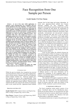

© Copyright 2026