1. No category

Lecture 6
Fourier Analysis: Applied Concepts
This lecture focuses on the application of Fourier analysis to real-world signals, which are
usually non-periodic, finite-length, and causal.
6.1
The Discrete Fourier Transform
The discrete Fourier series (DFS), introduced in the previous lecture, showed that an infinitely
long and periodic signal can be represented as a finite sum of complex exponentials. In this
section we introduce the discrete-time discrete Fourier transform (DT DFT, or simply DFT).
The DFT is very useful in practice since it is used for finite length sequences, which are usually encountered in real-world experiments.
Let {x[n]} be a sequence with finite length N and let xe [n] = x[n mod N ] for all n. The
sequence xe is known as the periodic extension of x. Note that xe is periodic with period N
and can therefore be represented by its DFS:
xe [n] =
where Xe [k] =
N −1
2π
1 X
Xe [k]ejk N n
N
k=0
N
−1
X
for all n,
2π
xe [n]e−jk N n
for all k.
n=0
The original sequence x is of finite length N and only defined for n = 0, . . . , N − 1. The DFS
representation of the signal’s periodic extension is valid for all n, and thus still holds over this
reduced interval. The sequence x can therefore be represented as
x[n] =
N −1
2π
1 X
X[k]ejk N n
N
for n = 0, . . . , N − 1,
k=0
where X[k] =Xe [k] =
N
−1
X
2π
x[n]e−jk N n
for k = 0, . . . , N − 1.
n=0
The sequence {X[k]} are known as the DFT coefficients of the signal. Furthermore, as we
have seen above, the DFT coefficients of a finite-length signal are the DFS coefficients of the
signal’s periodic extension.
Updated: October 30, 2014
1
6.1.1
The fast Fourier transform
Although mathematically simple to describe, direct calculation of the DFT is a very inefficient method of computing the transformation, and is thus rarely used in practice. Instead,
based on properties of the signal (eg. real-valued, even length, power of two length), many
simplifications and optimizations can be made to drastically reduce the number of operations
required to compute the DFT. The fast Fourier transform (FFT) refers to any such efficient
implementation.
Example (of a FFT calculation when N is even)
Let WN := e−j(2π/N ) , and let the signal x be of finite length N , where N is even. The DFT
coefficients are
X[k] =
N
−1
X
x[n]WNkn .
n=0
For each coefficient, the number of multiplications is N and the number of additions is N − 1.
Since there are N coefficients, the total number of multiplications is N 2 and the total number
of additions is N 2 − N .
The DFT can, however, be calculated in a more efficient way. Let
x0 [n] = x[2n],
x1 [n] = x[2n + 1],
n = 0, 1, . . . , N/2 − 1,
where x0 and x1 are sequences of length N/2. The respective DFT coefficients are
N/2−1
X0 [k] =
X
kn
x0 [n]WN/2
,
n=0
N/2−1
X1 [k] =
X
kn
x1 [n]WN/2
.
n=0
In this case, the total number of multiplications is 2(N/2)2 = N 2 /2, and the total number of
additions is 2(N/2)(N/2 − 1) = N 2 /2 − N .
Note that WN/2 = WN2 . Therefore, the DFT coefficients X0 and X1 can be rewritten as
N/2−1
X0 [k] =
X
x[2n]WN2kn ,
n=0
N/2−1
X1 [k] =
X
(2n+1)k
x[2n + 1]WN
WN−k .
n=0
It is then easy to show that
X[k] =X0 [k] + WNk X1 [k].
For each of the N coefficients, one additional multiplication and one additional addition
are required. Therefore, the total number of multiplications needed to compute the N DFT
coefficients X[k] is N 2 /2 + N and the total number of additions is N 2 /2. For large N , the
DFT can thus be calculated with half the calculations required with a direct implementation.
2
Example (of a FFT calculation when N is a power of 2)
Let the signal x be of finite length N , where N is a power of 2. In this case, the above process
can be repeated M = log2 N times. Focusing on multiplication (a similar result holds for
addition), we have:
1. X[k] = X0 [k] + WNk X1 [k]
2. X0 [k] = X00 [k] +
X1 [k] = X10 [k] +
..
3.
.
→ N multiplications
k
X01 [k]
WN/2
k
WN/2 X11 [k]
→ N/2 multiplications
→ N/2 multiplications
Each of the M steps requires N multiplications. Therefore, the required number of multiplications to compute the N coefficients X[k] is N log2 N , which is significantly smaller than N 2 :
N = 103
6
N = 10
6.2
N 2 = 106
2
12
N = 10
N log2 N ≈ 104
100 times smaller
7
50,000 times smaller
N log2 N ≈ 2 × 10
The Effect of Causal Inputs
We have previously seen that complex exponentials of the form ejΩn are eigenfunctions of an
LTI system G:
G{ejΩn } = H(ejΩ ){ejΩn },
where H(z) is the transfer function of system G, and H(ejΩ ) = H(z)z=ejΩ . Note that the
input signal has bi-infinite length (u[n] = ejΩn for all n ∈ (−∞, ∞)). We now investigate the
effects of applying a causal input sequence u, as would be the case in a real-world experiment.
Let u be defined as:
(
ejΩn
u[n] =
0
n≥0
n < 0,
and let y = Gu be the resulting output. In general, it is not true that
(
H(ejΩ )ejΩn n ≥ 0
y[n] =
0
n < 0.
However, we have the following useful result:
Theorem
Let
(
ejΩn
u[n] =
0
n≥0
n < 0.
Let the LTI system G be stable, and let y = Gu. Then
y[n] → H(ejΩ )ejΩn as n → ∞.
3
Proof
Let the LTI system G be stable, and let
(
ejΩn
u[n] =
0
(
0
v[n] =
ejΩn
n≥0
n<0
y = Gu
n≥0
n<0
w = Gv.
It is clear that {u[n] + v[n]} = {ejΩn }. By linearity, we have
{y[n] + w[n]} = G{u[n] + v[n]}
= G{ejΩn }
= H(ejΩ ){ejΩn }.
It follows that w[n] = H(ejΩ )ejΩn − y[n]. From w = Gv and since v[n − k] = 0 for k ≤ n, we
have that
w[n] =
=
∞
X
h[k]v[n − k]
k=−∞
∞
X
h[k]v[n − k].
k=n+1
Therefore
∞
X
|w[n]| = h[k]v[n − k]
≤
∴ |H(ejΩ )ejΩn − y[n]| ≤
k=n+1
∞
X
|h[k]||v[n − k]|
k=n+1
∞
X
|h[k]|,
k=n+1
since |v[n − k]| = 1 for all k > n. Since G is stable,
∞
X
k=−∞
|h[k]| < ∞ ⇒
∞
X
|h[k]| → 0 as n → ∞,
k=n+1
and therefore
|H(ejΩ )ejΩn − y[n]| → 0 as n → ∞
⇒
y[n] → H(ejΩ )ejΩn as n → ∞,
as required. Note that G does not have to be causal in the above theorem; however, in practice,
it is.
4
6.3
The DFT of Non-Periodic Signals
In this lecture, we have seen that there is a correspondence between the DFS and the DFT. It
follows that the coefficients {X[k]} of a sequence’s N -point DFT will exist at finite frequencies
Ω = k 2π
N for k ∈ [0, N − 1]. In this section, we investigate the DFT coefficients of periodic
and non-periodic signals.
Consider the complex exponential sequence {x[n]} = {ejΩ0 n }. We have shown in previous
lectures that its Fourier transform is given by
X(Ω) = 2πδ(Ω − Ω0 ).
2π
If Ω0 is an integer multiple of 2π
N , there exists a k0 ∈ [0, N − 1] such that k0 N = Ω0 . In this
case, the DFT coefficient X[k0 ] is located at the location of the delta function and captures
all of the signal’s power. Consider now the case where Ω0 is not an integer multiple of 2π
N,
which can happen for two reasons: N is not large enough; or the signal is simply not periodic
(the case for most real-world signals). In this case, the signal’s power is spread over all DFT
components. We illustrate this in the following example.
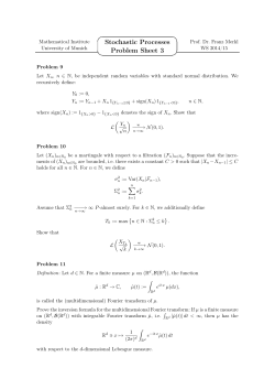
Example
Let {x[n]} = {ejΩ0 n } with Ω0 = π3 , and let X(Ω) = 2πδ(Ω − Ω0 ) be the DT Fourier transform of x. We choose to take a DFT of the first N = 12 samples of x. That is, let
xN [n] = x[n] for n = 0, . . . , N − 1, and let {X[k]} be the N -point DFT of {xN [n]}.
The following figure shows the locations of the N DFT coefficients and the location of the
Fourier transform’s delta function at Ω = Ω0 . Note that X[2] is at the same location as the
delta function, since k 2π
N = Ω0 for k = 2.
Im(z)
X[3]
X[4]
X[2]
X(Ω0 )
X[5]
Ω0
X[1]
2π
N
X[6]
X[0]
X[7]
X[11]
X[8]
X[10]
X[9]
5
Re(z)
Considering the magnitude of the DFT coefficients {X[k]}, we see that the power of the
sequence {xN [n]} is concentrated in the single DFT coefficient X[2]:
|X[k]|
12
8
4
0
0π
6
1π
6
2π
6
3π
6
4π
6
5π
6
6π
6
7π
6
8π
6
9π
6
10π
6
11π
6
Ω
Now let N = 10, xN [n] = x[n] for n = 0, . . . , N − 1, and let {X[k]} be the N -point DFT
of {xN [n]}. Note that Ω0 is not an integer multiple of 2π
N and thus no DFT coefficients exist
at the location of the delta function.
Im(z)
X[3]
X[2]
X[4]
X[1]
X(Ω0 )
Ω0
2π
N
X[5]
X[0]
X[6]
Re(z)
X[9]
X[7]
X[8]
Since no DFT coefficient exists at the location of the delta function, the power of the signal
is spread across all DFT coefficients:
|X[k]|
12
8
4
0
0π
5
1π
5
2π
5
3π
5
4π
5
5π
5
6
6π
5
7π
5
8π
5
9π
5
Ω
6.4
Aliasing
We saw that, in discrete time, a signal can be expressed as a sum of sinusoids:
Zπ
1
x[n] =
2π
X(Ω)ejΩn dΩ.
−π
A similar result holds in continuous time:
Z∞
1
x(t) =
2π
X(ω)ejωt dω.
−∞
Since sampling is a linear process, to understand the effects of sampling on a CT signal, it
suffices to explore what effect it has on one component.
In particular, consider x(t) = ejωt . When sampled with sampling period Ts , it becomes the
following DT signal:
{x[n]} = {ejΩn }, where Ω = ωTs .
But because ejΩn is periodic in Ω, with period 2π, the following different CT signals all
become the same when sampled:
2πk
x(t) = ej(ω+ Ts )t , where k is any integer.
Therefore, if we want to maintain a one-to-one relationship between a CT signal and its sampled version, we must restrict the frequency range of the CT signal to a width of 2π
Ts , and
ensure that the components do not overlap when sampled.
One common way of doing this is as follows:
π
π
− <ω< .
Ts
Ts
In particular, if we can ensure that ω ∈ (− Tπs , Tπs ), then when x(t) is sampled with sampling
period Ts , there is a one-to-one correspondence between the DT signal {x[n]} = {ejωTs n } and
x(t) = ejωt .
In general, given a DT signal {x[n]} (not necessarily a complex exponential sequence), one
can reconstruct the CT signal that generated it as follows:
X(Ω) =
x(t) =
∞
X
x[n]e−jΩn
n=−∞
π
ZTs
Ts
2π
X(Ω = ωTs )ejωt dω,
π
−T
s
where Ts is the sampling period, and it is assumed that the CT signal that generated {x[n]}
had all of its frequency content in the range |ω| < Tπs .
In fact, other ranges of width
2π
Ts
will work. For example,
7
•
π
Ts
< ω < 3π
Ts also gives a one-to-one correspondence, but is not very useful since it
excludes real-valued signals: As in DT, the continuous Fourier transform X(ω) of a real
signal x(t) must satisfy X(−ω) = X ∗ (ω).
•
π
Ts
< |ω| < 2π
Ts also gives a one-to-one correspondence. It is, however, not commonly
used because 0 is not in the range, thus excluding constant signals.
Example (Sampling a CT sinusoid)
Consider the CT sinusoid given by
x(t) = cos(ωt).
The signal is sampled with sampling period Ts = 1, resulting in the DT signal
x[n] = cos(Ωn),
where Ω = ωTs = ω. We will now see what happens for different values of ω. Let ω = π/10:
Now, consider the following two examples: ω = π − π/10 and ω = π + π/10.
The CT sinusoids are different, but the sampled DT sequences are the same, as shown by the
overlap of the two plots:
8
This shows that different CT frequencies can map to the same DT frequency. This is very
evident in the following example, where ω = 2π.
In this case, a CT frequency of ω = 2π corresponds to the DT frequency Ω = 0 and the
sampled signal is indistinguishable from a constant.
To summarize, aliasing is the effect of multiple CT frequencies mapping to the same DT
frequency. It is usually avoided by ensuring that all the signal’s frequency content is in the
range |ω| < Tπs . The frequency Tπs is called the Nyquist frequency and is in radians per second.
In Hertz, it is given by 2T1 s .
9