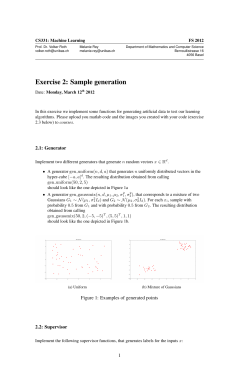
Automatica 45 (2009) 851–862
Contents lists available at ScienceDirect
Automatica
journal homepage: www.elsevier.com/locate/automatica
Harmonic analysis of pulse-width modulated systemsI
Stefan Almér ∗ , Ulf Jönsson
Optimization and Systems Theory, Royal Institute of Technology, 10044 Stockholm, Sweden
article
info
Article history:
Received 4 January 2008
Received in revised form
30 August 2008
Accepted 22 October 2008
Available online 22 January 2009
Keywords:
Pulse-width modulation
Harmonic analysis
Dynamic phasors
Periodic systems
Switched-mode circuits
a b s t r a c t
The paper considers the so-called dynamic phasor model as a basis for harmonic analysis of a class of
switching systems. The analysis covers both periodically switched systems and non-periodic systems
where the switching is controlled by feedback. The dynamic phasor model is a powerful tool for exploring
cyclic properties of dynamic systems. It is shown that there is a connection between the dynamic phasor
model and the harmonic transfer function of a linear time periodic system and this connection is used to
extend the notion of harmonic transfer function to describe periodic solutions of non-periodic systems.
© 2008 Elsevier Ltd. All rights reserved.
1. Introduction
The paper investigates the use of the so-called dynamic phasor
model (DPM) as a tool for harmonic analysis of a class of switching
systems. The systems considered are a class of pulse-width
modulated (PWM) systems that switch between subsystems in a
given order. In open loop, the switching is periodic and the PWM
systems are linear time periodic (LTP). In the closed loop case
the switching instants are determined by feedback of sampled
values of the state. In closed loop, the PWM systems are no longer
periodic. However, the pulses that excite the system begin at
periodically repeated time instants and the non-periodic systems
retain a cyclic property which is explored in the analysis.
The analysis is motivated mainly by switched-mode power
converters. Such devices can cause excessive harmonics in power
systems and may lead to instability (Möllerstedt & Bernhardsson,
2000). To be able to predict harmonics in switched-mode circuits
is important also in micro-electronics. Switched converters are
used extensively in portable radio frequency (RF) amplifiers (in
e.g., cellular phones) to increase efficiency and save power (Sahu &
Rincón-Mora, 2004). However, for RF devices there are strict limits
on the disturbance brought to neighboring channels. Spurious
I This work was supported by the Swedish Research Council and by the European
Commission research project FP6-IST-511368 Hybrid Control (HYCON). The material
in this paper was partially presented at IFAC 2008, Seoul, South Korea. This paper
was recommended for publication in revised form by Associate Editor Mario Sznaier
under the direction of Editor Roberto Tempo.
∗ Corresponding author. Tel.: +46 8 790 7504; fax: +46 8 225320.
E-mail addresses: [email protected] (S. Almér), [email protected] (U. Jönsson).
0005-1098/$ – see front matter © 2008 Elsevier Ltd. All rights reserved.
doi:10.1016/j.automatica.2008.10.029
frequency content caused by switched converters is therefore a
major concern in circuit design. Conventionally, harmonic analysis
of switched circuits is done with extensive simulations and the
FFT. Part of the contribution of this paper is to provide a tool for
harmonic analysis which may facilitate circuit verification.
The DPM is a powerful tool for exploring cyclic properties of
dynamic systems. It is obtained from a Fourier series expansion
of the system state over a moving time-window. It yields an L2 equivalent representation of the system in terms of an infinite
dimensional dynamic system which describes the evolution of
the time dependent Fourier coefficients (also known as dynamic
phasors).
To our knowledge, the DPM was introduced in the field of
power electronics as a tool for modeling the transients of switched
converters, see e.g., Caliskan, Verghese, and Stanković (1999)
and Sanders, Noworolski, Liu and Verghese (1991). It has also
been used for stability analysis (van der Woude, de Koning, &
Fuad, 2003) and for efficient simulation of switched converters,
see Maksimović, Stanković, Thottuvelil, and Verghese (2001) and
the references therein.
The DPM is conceptually appealing but poses some mathematical difficulties. The main problem is that the Fourier series expansion of the system state over a given time-window in general
does not converge uniformly. These convergence problems and the
corresponding differentiability problems are revealed in Tadmor
(2002) which provides useful analysis tools. The paper (Tadmor,
2002) derives conditions for the existence of a steady state solution to the phasor system. The current paper also contains results
on the existence of solutions to fixed point equations, but for a different situation. We consider the presence of an external disturbance of arbitrary frequency with the intention of establishing an
input–output mapping in the frequency domain.
852
S. Almér, U. Jönsson / Automatica 45 (2009) 851–862
In open loop, the PWM systems are LTP and the corresponding
DPM is an infinite dimensional time invariant system. In the
closed loop case however, the phasor system is not only infinite
dimensional but also nonlinear and it depends on sampled values
of the state with a delay. To obtain a tractable model we consider
a truncated averaged approximation of the phasor system. The
averaging and truncation yield a hierarchy of finite dimensional
nonlinear systems that become increasingly more accurate as the
size of the truncation increases. It is shown that the approximation
error can be made arbitrarily small provided that the switch period
is small enough and the truncation is large enough.
For harmonic analysis of the open loop (LTP) systems we
review some results on the so-called harmonic transfer function
(HTF) (Bittanti & Colaneri, 1999; Möllerstedt, 2000; Sandberg,
Möllerstedt, & Bernhardsson, 2005; Wereley & Hall, 1990; Zhou &
Hagiwara, 2001, 2002; Zhou, Hagiwara, & Araki, 2002) and provide
a time domain interpretation. The HTF generalizes the concept of
transfer function to LTP systems and is thus an efficient tool for
illustrating the frequency coupling between input and output. We
show that the HTF and the DPM are connected in the sense that the
DPM yields an explicit expression for the HTF.
For harmonic analysis of the closed loop PWM systems we
linearize the plant and derive an (approximate) HTF which is
analogous to the HTF of a LTP system. It is not obvious how to
linearize the closed loop PWM system, especially since we consider
sampled feedback. In our approach we rely on the truncated
averaged phasor system. This model accounts for the harmonics
generated by switching, but is still continuous and therefore
suitable for linearization.
The approximate phasor model represents the PWM system in
terms of dynamic phasor coefficients which capture the inherent
periodicity caused by switching. We assume that the approximate
phasor model is subjected to a periodic disturbance and that the
corresponding response is also periodic. The harmonics of the
phasor model is represented by (static) Fourier coefficients which
are determined by harmonic balance equations. We prove that
the harmonic balance equations have a solution provided that
the disturbance is small enough and we obtain an approximate
solution by linearizing the equations. The linearized harmonic
balance equations provide an approximate HTF for the closed loop
system. This HTF describes the steady state response of the nonperiodic PWM system to periodic disturbances.
The analysis techniques discussed in this paper are applied to
a realistic example; a step-up DC–DC converter. The steady state
response to a periodic disturbance is approximated for both open
and closed loop operation and the predicted responses are verified
by simulations in MatlabTM . The approximated and simulated
responses correspond well and the approximations capture the
nonlinear phenomena caused by switching.
Notation
In this paper L2 [−T , 0] denotes the set of square integrable
functions x : [−T , 0] → Rn with inner product
hx, yiL2 =
1
T
0
Z
x(τ )0 y(τ )dτ
−T
1/2
and norm kxkL2 = hx, xiL2 . l2 denotes the set of square summable
n
¯ k = x−k where
sequences x = {xk }∞
k=−∞ where xk ∈ C satisfies x
x¯ k is the complex conjugate of xk . The set is equipped with inner
product
hx, yil2 =
∞
X
x∗k yk
k=−∞
1/2
and norm kxkl2 = hx, xil2 . l2,N is the finite subspace of l2 where
xk = 0, ∀|k| > N. When the vector space is clear form context,
Fig. 1. Synchronous boost converter with external disturbance w in the source
voltage.
the subindices of k · kL2 and k · kl2 are often dropped. The Euclidean
norm is denoted |·|. For any bounded signal x(t ) we define kxk∞ =
supτ |x(τ )| and kxkt ,∞ = supτ ∈[t −Ts ,t ] |x(τ )| where Ts > 0.
πN denotes both a projection on l2 and a truncation as follows:
Firstly, πN : l2 → l2 is defined by the relation
(πN x)k =
xk , |k| ≤ N
0, |k| > N .
Secondly, πN : l2 → l2,N is defined by the relation (πN x)k =
xk , −N ≤ k ≤ N. The interpretation of πN will be clear from
context. The transformation T maps a complex valued sequence
ξ = {ξk }∞
k=−∞ to a doubly infinite dimensional block Toeplitz
matrix according to

..
.



T [ξ ] = 
. . .


..
.
ξˇ0
ξˇ−1
ξˇ−2
..
.
ξˇ1
ξˇ0
ˇξ−1
..
.
..
ξˇ2
ξˇ1
ξˇ0
.




. . .



..
.
where ξˇk = ξk In if ξk is scalar and ξˇk = ξk otherwise. TN [ξ ] is a
finite dimensional matrix consisting of the 2N + 1 central blocks
∗
∗
of T [ξ ]. col{ξk } = [. . . ξ1∗ ξ0∗ ξ−
1 . . .] is an infinite dimensional
column vector where ξk appear in descending order. I is used
for the identity operator on both finite and infinite dimensional
spaces. We use σ¯ to denote the maximum singular value of a matrix
and ⊗ is the Kronecker product.
2. Harmonic analysis; a motivating example
The paper considers harmonic analysis of a general class of
PWM systems. The analysis is motivated mainly by switchedmode DC–DC converters. As a motivating example we consider
the synchronous step-up (boost) converter (Schlecht, Kassakian,
& Verghese, 1991) shown in Fig. 1. The purpose of the boost
converter is to transform the source DC voltage vs into a DC voltage
at a reference level vref > vs which is to be supplied to the load. The
source voltage is transformed by switching the switch between onmode (s = 1) and off-mode (s = 0) at high frequency.
Defining ξ = [il , vc ]0 where il is the inductor current and vc is
the capacitor voltage the converter dynamics are
ξ˙ (t ) = (A0 + s(t )A1 ) ξ (t ) + B0 + D0 w(t )
where w is the disturbance in the source voltage and
 1

ro rc
1 ro
" vs #
−
rl +
−
 xl

r
+
r
x
r
+
r
o
c
l o
c
A0 = 
B0 = xl
,
1
ro
1
1
0
−
xc ro + rc
xc r o + r c
(1)
 1 rr

1 ro
"1#
o c

xl ro + rc  ,
A1 =  xl1ro +r rc
D0 = xl

o
0
−
0
xc r o + r c
and where s(t ) ∈ {0, 1} is the switch function.
We consider the case where the switch is controlled using fixed
frequency switching. This means that the time axis is partitioned
S. Almér, U. Jönsson / Automatica 45 (2009) 851–862
into intervals [kTs , (k + 1)Ts ] where k ∈ N and Ts > 0 is the
switch period. At the beginning of each switch interval a duty cycle
dk ∈ [0, 1] is chosen. The duty cycle determines the fraction of
time the switch is in the on-mode; at time kTs the switch turns
on. It remains on until time (k + dk )Ts when it turns to off-mode
and remains off until time (k + 1)Ts where a new duty cycle is
determined and the procedure is repeated.
Ideally, the converter attains a periodic solution ξ 0 (t ) =
0
ξ (t + Ts ) when the duty cycle is constant so that dk = d0 ∀k.
For a properly designed boost converter, the voltage part of the
periodic solution will have small ripple and a dominant DC part
at approximately vs /(1 − d0 ).
In many applications it is not sufficient to keep the duty cycle
constant. Variations in the source voltage and the load imply
that the duty cycle must be varied to keep the output voltage
constant at the reference level. In other words, the duty cycle must
be determined by feedback. In practice, the duty cycle is often
determined by sampled values of the state according to
d0 + F (ξ (kTs ) − ξ 0 (kTs ))
(2)
dk = sat[0,1]
where F is a feedback vector and sat[0,1] denotes the saturation
between zero and one.
We consider the boost converter in closed loop operation and
state the following problem: Given a disturbance w with a certain
spectrum, what is the spectral content of a certain output signal?
This is a highly complicated problem due to the nonlinear and
discontinuous nature of the system. We will address this problem
by first embedding the dynamics of the boost converter in a general
class of pulse-width modulated switching systems in Section 3. To
capture the harmonic content in the system signals we introduce
the dynamic phasor model in Section 4 and prove in Theorem 1 that
it can be approximated by the dynamics of a continuous nonlinear
finite dimensional system. This allows us to determine the spectral
contents using harmonic balance techniques in Section 5, where
we show in Theorem 2 that a certain closed loop harmonic transfer
function can be used to approximate solutions to the nonlinear
harmonic balance equation.
3. A class of switching systems
The paper considers a class of PWM systems which is
particularly suited to model switched-mode power converters. The
systems switch between subsystems in a given order and are of the
form
ξ˙ (t ) = (A0 + s(t )A1 ) ξ (t ) + B0 + s(t )B1 + (D0 + s(t )D1 ) w(t )
(3)
ζ (t ) = C (t )ξ (t )
where ξ (t ) ∈ Rn , w(t ) : R → Rm is an external disturbance
assumed to be in L2 [t0 , t1 ] for any finite time interval [t0 , t1 ], Ai ∈
Rn×n , Bi ∈ Rn , Di ∈ Rn×m are constant matrices, C (t ) ∈ Rp×n is a
Ts -periodic matrix and s is the PWM function
s(t ) =
1,
0,
t ∈ [kTs , (k + dk )Ts )
t ∈ [(k + dk )Ts , (k + 1)Ts ).
We denote the deviation from ξ 0 as x := ξ −ξ 0 and in what follows
we consider the error dynamics
x˙ (t ) = (A0 + s(t )A1 ) x(t ) + s(t ) − sd0 (t )
× A1 ξ 0 (t ) + B1 + (D0 + s(t )D1 ) w(t )
=: A(t )x(t ) + B(t ) + D(t )w(t )
y(t ) = C (t )x(t )
Assumption 1. Consider the unperturbed system (3) where w ≡
0. There exists at least one point (ξ0 , d0 ) ∈ Rn × [0, 1] such
that (3) attains a Ts -periodic solution ξ 0 (t ) = ξ 0 (t + Ts ) when
the initial condition is ξ (0) = ξ0 and the duty cycle is constant,
i.e., dk = d0 ∀k.
dk = sat[0,1]
1
d0 +
Ts
kTs
Z
(k−1)Ts
F (τ )x(τ )dτ
(6)
where sat[0,1] denotes the saturation between zero and one and
where the feedback vector F (t ) is of the form
F (t ) =
N
X
ejkωs t Fk
k=−N
where ωs = 2π /Ts and where Fk ∈ Rn satisfy Fk = F−k . We note
that if Fk = F ∀k, then the feedback (6) is an approximation of the
sampled feedback (2) which is often used in practice, see Almér
(2008) for details. We also note that the integral in (6) implies that
the feedback can be expressed as a linear function of the dynamic
phasor coefficients defined in (7). It is thus easily represented in
the DPM (9) defined below.
4. The dynamic phasor model
We use the idea of Sanders et al. (1991) and Caliskan et al.
(1999) to represent the solution of (5) in the frequency domain
where we can distinguish how the various harmonics develop over
time. The nth phasor (Fourier coefficient) of x is defined as
hxin (t ) =
1
t
Z
Ts
x(τ )e−jnωs τ dτ
(7)
t −Ts
where ωs = 2π /Ts . Note that the phasors are defined over a
moving time-window and are thus time dependent. Note also that
if x is periodic with period Ts , then hxin (t ) is constant. As was
remarked above, the solution x of (5) is absolutely continuous. This
implies that the sequence {hxin (t )}∞
n=−∞ is in l2 for all t. For brevity,
the time dependence of the phasors is often suppressed.
The time domain signal x is reconstructed on the interval [t −
Ts , t ] according to
∞
X
x(t , τ ) =
hxin (t )ejnωs (t +τ ) ,
τ ∈ [−Ts , 0].
(8)
n=−∞
Note that x(t ) 6= x(t , τ ), but the equality x(t + τ ) = x(t , τ ) holds
a.e. on the set {τ | τ ∈ [−Ts , 0]}.
Using partial integration one can show that the phasor
coefficients satisfy
d
dt
hxin =
d dt
x
n
− jnωs hxin .
Introducing the notation
ξˆ 0 = col{ ξ 0 n },
sˆ = col{hsin },
sˆd0 = col{ sd0 n }
F = (F−N , . . . , F0 , . . . , FN )
xˆ = col{hxin },
1 The assumption is natural for switched converters as such systems are typically
designed to have periodic solutions.
(5)
where sd (t ) is defined according to (4) with the duty cycle fixed at
d (dk = d ∀k). Note that sd (t ) is a periodic function but s(t ) need
not be periodic. It can be shown that (5) has a unique absolutely
continuous solution for every initial condition.
The duty cycle dk is determined by sampling a weighted average
of the state. The feedback is of the form
(4)
Here, Ts > 0 is the period time, k ∈ N and dk ∈ [0, 1] is
the duty cycle. The duty cycle determines the fraction of time
each mode is active and thus controls the system dynamics. The
unperturbed system (where w ≡ 0) is assumed1 to satisfy the
following assumption.
853
w
ˆ = col{hwin }
854
S. Almér, U. Jönsson / Automatica 45 (2009) 851–862
the phasor dynamics can be written in the compact form
d
dt
ˆ (ˆs)w
xˆ = (−jωs Eˆ n + Aˆ (ˆs))ˆx + Bˆ (ˆs − sˆd0 ) + D
ˆ
(9)
yˆ = Cˆ xˆ
dk = sat[0,1] (d0 + F πN xˆ (kTs ))
where
Eˆ n = blkdiag(. . . , 2In , In , 0, −In , −2In , . . .)
Aˆ (ˆs) = I ⊗ A0 + (I ⊗ A1 )T [ˆs]
(10)
Bˆ = I ⊗ B1 + (I ⊗ A1 )T [ξˆ 0 ]
and where Cˆ = T [C (t )]. Note that the feedback (6) corresponds
to sampling the 2N + 1 low order phasors hxin and that sˆ depends
on these samples.
In the open loop case (where the duty cycle is constant and
equal to d0 ), T [ˆs] is constant and the affine term Bˆ (ˆs − sˆd0 )
disappears. In this case the time periodic switched system (5) is
represented by a linear time invariant system in the frequency
domain. However, when s is determined by the feedback (6), the
DPM (9) is an infinite dimensional, nonlinear system that depends
on the sampled state with a delay. To obtain a tractable model we
introduce an approximation in two steps:
In the first step we replace the phasor coefficients hsin with the
nonlinear averaged approximation
sav,n (d) =
d,
n=0
j
−jn2π d
(11)
(e
− 1), n 6= 0.
n2π
which is the nth Fourier coefficient of a square wave with constant
duty cycle equal to d. In other words, if the duty cycle is fixed so
that dk = d ∀k, then hsin (t ) = hsd in (t ) = sav,n (d). This implies
that if the duty cycle varies slowly (compared to the switch period
Ts ), then sav,n (d) is a good approximation of hsin .
In the second step we truncate the infinite state vector to obtain
a finite dimensional system which approximates the low order
phasor coefficients. We also describe the dynamics as a function of
the deviation δ := d − d0 from the stationary duty cycle. For a fixed
integer N ≥ 0 the approximation of the phasors hxi−N , . . . , hxiN
is given by the system
d
dt
Theorem 1. Consider the DPM (9) and let w be the signal
corresponding to the phasor vector w
ˆ . Let xˆ (t ) be the solution with
xˆ (t0 ) = 0 and let Z(t ) be the solution of the approximate system (12)
with Z(t0 ) = 0. Define the approximation error as
eˆ := (ˆe1 , eˆ 2 ) ∈ l2,N × l2,N¯
ˆ (ˆs) = I ⊗ D0 + (I ⊗ D1 )T [ˆs]
D
(
function of d whereas hsin is determined by the samples dk =
d(kTs ) of d.
When the switch period Ts is small, the system (12) provides a
good approximation of the DPM. To prove this claim we now show
that the solutions xˆ and Z are close on infinite time intervals. Since
the approximation Z is finite dimensional, it is natural to define
the error in two components in the next theorem.
Z = (−jωs N + A(δ))Z + BS (δ) + D (δ)W
Y = CZ
(12)
δ = sat[−d0 ,1−d0 ] (F Z)
where C = πN Cˆ πN , B = πN Bˆ πN , W = πN w
ˆ and
N = blkdiag(NIn , . . . , In , 0, −In , . . . , −NIn )
A(δ) = πN Aˆ (Sav (δ))πN
ˆ (Sav (δ))πN
D (δ) = πN D
(13)
S (δ) = πN (Sav (δ) − Sav (0))
where eˆ 1 := πN xˆ − Z and eˆ 2 := (I − πN )ˆx and let the error norm
be kˆek := (|ˆe1 |2 + kˆe2 k2l2 )1/2 . Assume that the unforced approximate
system
d
dt
Z = (−jωs N + A(δ))Z + BS (δ)
δ = sat[−d0 ,1−d0 ] (F Z)
is (locally) exponentially stable. Under these assumptions there exists
a number rw > 0 s.t. if kwkL∞ < rw and kwk
˙ L∞ < rw , then
∀ > 0 ∃ T0 > 0 s.t. kˆe(t )k ≤ ∀t if Ts ≤ T0
where Ts is the switch period.
Proof. See Appendix A.
In the theorem above we assume that the unforced system (12)
is exponentially stable. A systematic procedure to verify stability
of (12) can be adopted from Almér and Jönsson (2007) and Almér,
Jönsson, Kao and Mari (2007).
5. Harmonic analysis
In Section 5.1 we review the HTF (Bittanti & Colaneri, 1999;
Möllerstedt, 2000; Sandberg et al., 2005; Wereley & Hall, 1990;
Zhou & Hagiwara, 2001, 2002; Zhou et al., 2002) and provide a time
domain interpretation. We also show that the DPM provides an
explicit formula for the HTF. In Section 5.2 we consider (5) in closed
loop (then the system is non-periodic) and use the approximate
phasor model to derive a harmonic transfer function which is
analogous to the HTF of a LTP system.
5.1. The harmonic transfer function; a review
LTP systems do not have the property of frequency separation
which is characteristic for LTI systems. If the input to a LTP system
is a sinusoid with frequency ω, the steady state output will be a
sum of sinusoids with frequencies ω + kωs where k ∈ Z and ωs
is the frequency of the system. The HTF generalizes the transfer
function to LTP systems and is thus a powerful tool for describing
the frequency coupling between input and output.
Consider the LTP system
x˙ (t ) = Ap (t )x(t ) + Dp (t )w(t )
(14)
Sav (δ) = col{sav,n (d0 + δ)}
y(t ) = Cp (t )x(t )
ˆ (·) are defined in (10).
where Aˆ (·), Bˆ (·) and D
where Ap , Dp and Cp are Ts -periodic matrices. Under loose
assumptions (Sandberg et al., 2005), the impulse response h of (14)
can be expanded in a Fourier series and the response y to the input
w can be expressed as the convolution
Remark 1. It should be noted that Z is an approximation of the
2N + 1 phasors hxi−N , . . . , hxiN in (9) and thus, Z ∈ C(2N +1)n .
The kth approximate phasor is denoted Z[k] ∈ Cn , k =
−N , . . . , N. Analogously, the kth approximate phasor of the output
is denoted Y[k].
The system (12) is a nonlinear differential equation and is therefore
tractable for analysis. The important distinctions from (9) is that
the state space is finite dimensional and that sav,n is a continuous
y(t ) =
Z
t
∞
X
hk (t − τ )ejkωs t w(τ )dτ
0 k=−∞
=
∞
X
k=−∞
hk (·)ejkωs (·) ∗ w(·)ejkωs (·) (t )
(15)
S. Almér, U. Jönsson / Automatica 45 (2009) 851–862
 
..
..
.
.

 
Y (ω + ωs ) 

 
 Y (ω)  = . . .
Y (ω − ω ) 
s 


..
.
..
.
|

H0 (ω + ωs )
H−1 (ω + ωs )
H−2 (ω + ωs )
..
.
H1 (ω)
H0 (ω)
H−1 (ω)
..
.
{z
..
H2 (ω − ωs )
H1 (ω − ωs )
H0 (ω − ωs )
H (ω)
.
855

..
.


W (ω + ωs )


 W (ω) 
W (ω − ω )
s 

..
.




. . .


..
.
}
Box I.
where hk are the Fourier coefficients of h. Let Y (ω) := (Fy)(ω),
W (ω) := (Fw)(ω) be the Fourier transform of the output and
input. Applying the Fourier transform to (15) one can express
Y (ω + nωs ), n ∈ Z as a function of W (ω + kωs ), k ∈ Z as shown
in Box I. In Box I, the doubly infinite matrix H (ω) is the harmonic
transfer function with entries Hk (ω) = (Fhk )(ω).
The HTF extends the concept of transfer function to LTP systems.
From the transfer function of a LTI system one can immediately
determine the response to a sinusoidal input and it can be shown
that the HTF has the corresponding property for LTP systems. The
steady state response to the input signal w(t ) = sin(ωt ) is
∞
P
y(t ) =
|Hk (ω)| sin((ω + kωs )t + φk )
(16)
k=−∞
where φk = arg Hk (ω).
An explicit formula for the HTF can be obtained from the DPM
corresponding to (14). To see this, let hwin be the nth phasor
coefficient of w . One can show that the Fourier transform of hwin
satisfies
(F hwin )(ω) = W (ω + nωs )
1 − e− j ω T s
jωTs
.
Using the relation (15) we can also derive the equality
(F hyin )(ω)
∞
X
1 − e−jωTs
Hk (ω + (n − k)ωs )W (ω + (n − k)ωs )
=
.
jωTs
k=−∞
By identifying F hwin−k in this expression we recognize that the
relation between F hwin and F hyin is given by the HTF, i.e.,
..
.

 (F hyi1 )(ω)

 (F hyi0 )(ω)
(F hyi )(ω)
−1

..
.

..
.



 (F hwi1 )(ω)


 = H (ω)  (F hwi0 )(ω)

(F hwi )(ω)
−1


..
.






.


dt
ˆ (ˆsd0 )w
xˆ = −jωs Eˆ n + Aˆ (ˆsd0 ) xˆ + D
ˆ
To estimate the effect of the disturbance on the system (5) we
consider the corresponding truncated averaged phasor model (12).
We assume that the approximate phasor system is subjected to
a periodic disturbance W and we assume that the steady state
response of the phasor coefficients is also periodic. To determine
the response of the phasor coefficients we state the corresponding
harmonic balance equations and suggest an approximate solution
to the nonlinear equations. A first order approximation where all
frequencies except the zero and first order terms are dropped
results in a harmonic transfer function that maps periodic
disturbances to the corresponding (approximate) periodic output.
We assume that the steady state response of (12) to a periodic
disturbance W (t ) with frequency ω is periodic with period
T = 2π /ω. In other words, we assume that
W (t ) =
∞
X
W k ejkωt ,
Z(t ) =
∞
X
By formally applying the Fourier transform to (17) we obtain an
explicit formula for the HTF H (ω) corresponding to the open loop
system (5)
(18)
Well posedness of the HTF is discussed in Sandberg et al. (2005) and
Zhou and Hagiwara (2002). Our derivation is strictly formal and is
merely used to show an analogy between the HTF of a LTP system
Zk ejkωt
δk ejkωt ,
Y (t ) =
∞
X
(19)
Yk ejkωt
k=−∞
is a periodic solution of (12). In Section 5.2.2 we show that
this assumption is valid for small disturbances W . Since δ(t ) is
periodic, A(δ(t )), S (δ(t )) and D (δ(t )) are also periodic and can
be represented by the Fourier series
A(δ(t )) =
∞
X
Ak ejkωt ,
S (δ(t )) =
k=−∞
D (δ(t )) =
(17)
∞
X
k=−∞
k=−∞
k=−∞
yˆ = Cˆ xˆ .
ˆ (ˆsd0 ).
H (ω) = Cˆ (jωI − (−jωs Eˆ n + Aˆ (ˆsd0 )))−1 D
5.2. A HTF approximation of the closed loop system
δ(t ) =
The relation above implies that the HTF of a LTP system can be
derived by applying the Fourier transform to the corresponding
DPM.
Consider the DPM of the open loop system (5), i.e.,
d
and the transfer function derived in Section 5.2. Our numerical
examples in Section 6 are based on a truncated version of (17),
which can be justified by the conclusions of Theorem 1.
In Section 5.2 we consider (5) in closed loop. In this case,
Theorem 1 implies that for small disturbances w , the truncated
phasor model (12) approximates the DPM arbitrarily well. The
approximate model (12) will next be used to extend the notion of
HTF to describe periodic solutions of the non-periodic closed loop
system (5).
∞
X
∞
X
Sk ejkωt
k=−∞
(20)
Dk ejkωt
k=−∞
where the Fourier coefficients Ak , Sk , Dk are functions of {δk }∞
k=−∞ .
We assume that the disturbance W is small enough so that the
feedback in (12) does not saturate and consider the harmonic
balance equations associated with the periodic solution (19). By
introducing the notation
ˆ = col{Zk },
Z
Yˆ = col{Yk },
δˆ = col{δk }
ˆ = col{Sk }
Sˆ(δ)
ˆEq = blkdiag(. . . , 2Iq , Iq , 0, −Iq , −2Iq , . . .)
Wˆ = col{W k },
856
S. Almér, U. Jönsson / Automatica 45 (2009) 851–862
where q = (2N + 1)n, the balance equations are written
ˆ Zˆ + Bˆ Sˆ(δ)
ˆ + Dˆ (δ)
ˆ Wˆ
ˆ = −jωs Nˆ + Aˆ (δ)
jωEˆ q Z
(21)
ˆ
Yˆ = Cˆ Z
δˆ = Fˆ Zˆ
where Nˆ = I ⊗ N , Cˆ = I ⊗ C , Fˆ = I ⊗ F , Bˆ = I ⊗ B and
ˆ = T [A(δ(t ))], Dˆ (δ)
ˆ = T [D (δ(t ))] are infinite block
where Aˆ (δ)
Toeplitz matrices. To find an approximate solution to the (highly
nonlinear) equations (21) we use a first order approximation of the
term Sav (δ) defined in (13). We have for n 6= 0
sav,n (d0 + δ(t )) ≈ sav,n (d0 ) + e−jn2π d
0
∞
P
δk ejkωt
k=−∞
where we used the approximation ex ≈ 1 + x. Since sav,0 (δ(t )) =
d0 + δ(t ) the approximation of Sav (δ) is
Sav (δ) ≈ Sav (0) + Ψ
∞
X
δk e
jkωt
= Sav (0) + Ψ δ(t )
k=−∞
where Ψ = col{e−j2π d n }. The approximation above is used to derive linear approximations (linear in δk ) of the Fourier coefficients
Ak , Sk , Dk . By using the linearity of TN [·] one can show that
0
A(0) + δ0 (I ⊗ A1 )TN [Ψ ],
ˆ
Ak (δ ) ≈
δk (I ⊗ A1 )TN [Ψ ], k 6= 0
where Hcl,0,0 denotes the central block of the matrix. It should
be noted that Hcl does not have the same structure as Box I. This
structure is lost because of the feedback and pulse modulation. The
matrix in (24) is of size (2N + 1)n × (2N + 1)n.
5.2.1. Connection to the time domain
Eq. (23) gives an approximate steady state response of the
approximate phasor model (12) in terms of a transfer function from
Fourier coefficients W k to Yk . In the section below we express the
corresponding time domain representation. For simplicity, we only
consider the case of a sinusoidal disturbance.
Let the disturbance in (5) be w(t ) = sin(ωt ) where ω ωs .
The phasors of w(t ) are approximated as hwi0 (t ) ≈ sin(ωt ) and
hwin (t ) ≈ 0 for n 6= 0. In other words, the truncated phasor
representation of w(t ) is approximately
W ( t ) = W − 1 e− j ω t + W 1 ej ω t
1
where W ±1 = [0, . . . , 0, ± 2j
, 0, . . . , 0]0 . The frequency separation property of (22) implies that the only nonzero coefficients in
Yˆ are Y1 and Y−1 . The approximate response of (5) to the sinusoidal disturbance is therefore given by
y(t ) ≈
k=0
D (0) + δ0 (I ⊗ D1 )TN [Ψ ],
δk (I ⊗ D1 )TN [Ψ ], k 6= 0
ˆ ≈
Dk (δ)
≈
k=0
efficients in (21) are replaced by the linear approximations above
and all cross terms are dropped. In other words, all products of δk ,
Zl and W m are removed from the equation. In doing so, we remove
the connection between Fourier coefficients of different order and
obtain the block diagonal system of equations
ˆ = −jωs Nˆ + Aˆ 0 Zˆ + Bˆ Ψˆ δˆ + Dˆ 0 Wˆ
jωEˆ q Z
Y1 ejωt + Y−1 e−jωt [n]ejnωs t
N
X
Hcl (ω)W 1 ejωt + Hcl (−ω)W −1 e−jωt [n]ejnωs t
n=−N
where Y[n] denotes the nth approximate phasor coefficient of y
(see Remark 1). We now use that only the zero coefficient of W ±1
is nonzero and that Hcl,n,0 (−ω) = Hcl,−n,0 (ω). It follows
y(t ) ≈
(22)
=
δˆ = Fˆ Zˆ
N
X
N
X
Hcl,n,0 (ω)
ej(ω+nωs )t
2j
− Hcl,n,0 (−ω)
e−j(ω−nωs )t
2j
|Hcl,n,0 (ω)| sin((ω + nωs )t + φn,0 )
(25)
n=−N
ˆ 0 = I ⊗ D (0).
where Ψˆ = I ⊗ ΨN , Aˆ 0 = I ⊗ A(0), Bˆ = I ⊗ B and D
The matrices in (22) are block diagonal and there is no
coupling between the Fourier coefficients. This means that the
approximation of the kth Fourier coefficient Zk is a linear function
of (only) the kth Fourier coefficient W k of the disturbance. The
relation is written
Yk = Hcl (kω)W k ∀k ∈ Z
(23)
where
Hcl (ω) = C (jωI − (−jωs N + A(0)) − B ΨN F )−1 D (0)
is a transfer function of dimension (2N + 1)n. As was noted
ˆ (ˆsd0 )πN and N =
above, A(0) = πN Aˆ (ˆsd0 )πN and D (0) = πN D
πN Eˆ n πN . In light of the expression (18) for the HTF, Hcl can be
seen as a truncated version of H with an additional term B ΨN F
representing the effect of the feedback. In the section below we use
the individual entries of Hcl . They are indexed as
Hcl (ω)
.



= . . .


..
=
n=−N
ˆ
Yˆ = Cˆ Z
..
N
X
n=−N
where A(0) = πN Aˆ (Sav (0))πN = πN Aˆ (ˆsd0 )πN , D (0) =
πN Dˆ (Sav (0))πN = πN Dˆ (ˆsd0 )πN and ΨN = πN Ψ . The Fourier co-

Y[n]ejnωs t
n=−N
ˆ ≈ δk ΨN
Sk (δ)
N
X
.
Hcl,1,1 (ω)
Hcl,0,1 (ω)
Hcl,−1,1 (ω)
..
.
Hcl,1,0 (ω)
Hcl,0,0 (ω)
Hcl,−1,0 (ω)
..
.
..
Hcl,1,−1 (ω)
Hcl,0,−1 (ω)
Hcl,−1,−1 (ω)
.
5.2.2. Existence of solution to the harmonic balance equations
To justify the assumption that the harmonic balance equations
have a solution we show that for small disturbances W this is
indeed the case. The harmonic balance equations (21) have a
solution iff there is a solution δˆ to
ˆ Wˆ + ∆
ˆ
ˆ 1 (δ)
ˆ 2 (δ)
δˆ = Fˆ H1 (ω)Dˆ 0 Wˆ + Fˆ H1 (ω) ∆
where
H1 (ω) = jωEˆ q − (−jωs Nˆ + Aˆ 0 ) − Bˆ Ψˆ Fˆ
−1
(26)
−1
ˆ = I − (Aˆ (δ)
ˆ − Aˆ 0 )H1 (ω)
ˆ − Dˆ 0
ˆ 1 (δ)
∆
Dˆ (δ)
−1 ˆ = I − (Aˆ (δ)
ˆ − Aˆ 0 )H1 (ω)
ˆ − Ψˆ δˆ .
ˆ 2 (δ)
∆
Bˆ Sˆ(δ)




. . .


..
.
where Hcl,n,k is the (n, k)-block of Hcl (see (24)) and where φn,0 =
arg Hcl,n,0 (ω). The expression above is analogous to the expression
given in Section 5.1 for the response of a LTP system to a sinusoidal
input.
(24)
ˆ 0 Wˆ is the
From (22) it is clear that the first term Fˆ H1 (ω)D
approximate solution given by the linearized harmonic balance
S. Almér, U. Jönsson / Automatica 45 (2009) 851–862
857
equations while the second term is a higher order function of δˆ . We
note that the operator H1 (ω) is block diagonal and can be written
H1 (ω) = blkdiag(. . . , H2 (ω), H2 (0), H2 (−ω), . . .)
where H2 (ω) = (jωI − (−jωs N + A(0)) − B ΨN F )−1 . It follows
that the operator jωEˆ q H1 is also block diagonal and the induced
l2 -norms satisfy
kH1 (ω)k = sup σ¯ (H2 (kω))
k∈Z
kjωEˆ q H1 (ω)k = sup σ¯ (jωkH2 (kω)).
Fig. 2. Harmonic transfer function H (ω) (left) and closed loop harmonic transfer
function Hcl (ω) (right) of the boost converter. The left plot shows the coefficients
Hk , k = −2, . . . , 2 as a function of frequency and the right plot shows the
coefficients Hcl,k,0 , k = −2, . . . , 2.
k∈Z
We note that an analogous equality holds for Fˆ H1 .
Let
ˆ Wˆ ) = Fˆ H1 (ω)
H (δ,
ˆ Wˆ + ∆
ˆ .
ˆ 1 (δ)
ˆ 2 (δ)
Dˆ 0 + ∆
(27)
There exists a solution to the harmonic balance equations (21) iff
ˆ Wˆ ).
there exists a solution to the fixed point equation δˆ = H (δ,
Clearly, for Wˆ = 0 there is the solution 0 = H (0, 0). We will show
that three is a solution also for nonzero disturbances Wˆ if they are
small enough. The claim is formalized in the following theorem.
Theorem 2. Let rw > 0 and let r > 0 be such that
sup σ¯ (A(δ) − A(0)) < 1/(2kH1 k)
(28)
|δ|<r
C1 (r )rw + C2 (r )r 2 < r
(29)
where Ci > 0 are defined as

C1 (r ) = kFˆ H1 k σ¯ (D (0)) +
+ σ¯ (D (0))) + c
1
√
√ + 2π
2r
γ22 + (γ1 (γ2 r
2 !1/2

2
√
C2 (r ) = kFˆ H1 k2 2c σ¯ (B ) 1 +

1
√ + γ1 r
2 !1/2
2 2
where
1/2
γ1 = c kH1 k2 + T 2 kjωEˆ q H1 k2
+ cT kjωEˆ q H1 k
γ2 = 2c (1 + kH1 kσ¯ (D (0)))
and where c > 0 is a constant satisfying
sup |S (δ) − ΨN δ| < cr 2
(30)
|δ|<r
sup |S 0 (δ) − ΨN | < cr
(31)
|δ|<r
sup σ¯ (A(δ) − A(0)) < cr
(32)
|δ|<r
sup σ¯ (D (δ) − D (0)) < cr
(33)
|δ|<r
sup σ¯ (A0 (δ)) < c
(34)
|δ|<r
sup σ¯ (D 0 (δ)) < c .
(35)
|δ|<r
Then the harmonic balance equations (21) have a solution for all Wˆ
2
such that 2(kWˆ k2l2 + T 2 kjωEˆ q Wˆ k2l2 ) ≤ rw
.
Proof. See Appendix B.
Remark 2. For r and rw small enough, the first term of (27) will
be dominating. From Theorem 2 we can thus infer that the linear
approximation provides an accurate prediction of a solution to the
harmonic balance equation (22). We may improve this solution
using a fixed point iteration but for the example in the next section
the improvement is negligible.
6. Example
To illustrate the theory presented in the paper we return to
the boost converter considered in Section 2. We use the results of
Section 5 to investigate the harmonic properties of this system in
both open and closed loop. Further examples can be found in Almér
and Jönsson (2007).
The system is on the form (3) with B0 = D0 = 0 and the
remaining system matrices defined in (1) We take C (t ) = [0, 1]
so that the capacitor voltage is the output signal. The dynamics
have been scaled to obtain switch period Ts = 1 and the parameter
values are expressed in the per unit system. They are xl = 3/10π
p.u., xc = 70/10π p.u., rl = 0.05 p.u., rc = 0.005 p.u., ro = 1 p.u.
and the source voltage is vs = 0.75 p.u. It should be noted that the
inductance and capacitance are chosen quite small. This is to make
the effect of the disturbance appear more clearly.
The reference output voltage is vref = 1. The stationary duty
cycle d0 is chosen to make the average output voltage equal to vref
and the corresponding periodic stationary solution is denoted ξ 0 .
The dynamics of the error x := ξ − ξ 0 is considered in both open
loop (i.e., dk = d0 ∀k) and in closed loop with the linear feedback (2)
with F = [−0.1021, 0.1555]. In the open loop case we consider
the DPM (17) corresponding to (5). The DPM is truncated and we
apply the Fourier transform to obtain a truncated HTF H (ω). The
gains |Hk (ω)| (see Box I for the definition) of H (ω) are plotted for
k = −2, . . . , 2 in Fig. 2.
In the closed loop case we consider the averaged dynamic
phasor system (12) and derive the corresponding closed loop
harmonic transfer function Hcl (ω). The gains |Hcl,k,0 (ω)| (see (24)
for the definition) of H (ω) are plotted for k = −2, . . . , 2 in Fig. 2.
The plots in Fig. 2 can be interpreted in the light of formulas (16)
and (25) which give the steady state response to a sinusoidal
disturbance. The formulas (16) and (25) imply that when the
system is subjected to a sinusoidal disturbance with angular
frequency ω, the output will be a sum of sinusoids with shifted
frequencies ω + kωs . The central plot (which has index zero) shows
the amplification of the fundamental term sin(ωt ) and the offdiagonal plots (with index k) show the amplitude of the additional
shifted frequencies sin((ω + kωs )t ). The fact that the off-diagonals
in Fig. 2 are nonzero explains why the responses plotted below are
not purely sinusoidal but contain ripple.
The harmonic transfer functions of the open and closed loop
systems are used in formulas (16) and (25) respectively to
approximate the steady state response to a sinusoidal disturbance.
We consider the disturbance w(t ) = a sin(2π ft ) where a = 0.1
and f = 0.1 Hz.
The approximate steady state responses predicted by the HTFs
are verified by simulation in Matlab. The predicted and simulated
steady state responses of the capacitor voltage are shown in Fig. 3.
This figure shows that in the open loop case, the HTF provides a
858
S. Almér, U. Jönsson / Automatica 45 (2009) 851–862
perfect match with the simulation. The harmonics caused by the
switching is clearly visible. These harmonics correspond to the offdiagonal elements of the HTF in Fig. 2. In the closed loop case
the match is not perfect, but the closed loop HTF still provides a
good approximation which accounts for the harmonics caused by
switching.
7. Conclusions
The dynamic phasor model was used as a tool for harmonic
analysis of a class of PWM systems. A connection between the
dynamic phasor model and the HTF of a LTP system was shown
and the notion of HTF was extended to describe periodic solutions
of the non-periodic PWM systems.
Acknowledgement
The authors would like to thank Dr. Sébastien Cliquennois for
valuable comments on possible applications to the theory in this
paper.
Appendix A. Proof of Theorem 1
The complete proof of Theorem 1 is rather lengthy since one
must consider both the truncation of the infinite dimensional state
and the averaging approximation. The main difficulty in the proof
is to provide a norm estimate of the difference sˆ − Sav (δ), between
the phasor vector of the PWM switching function in (4) and its
corresponding nonlinear approximation in (11). The difficulty lies
in that the former is determined by the duty ratio function (6),
which is determined at the sampling times kTs while the latter is
determined by the duty ratio function in (12) which is a continuous
function of the state. Because of space limitations we have omitted
the details on how the above mentioned difference is estimated
and simply state the result. See Almér (2008) for a complete proof.
In the proof below we use the following definitions
kAk := sup σ¯ A(s(t )),
s
kBk := sup σ¯ B(s(t ))
s
kDk := sup σ¯ D(s(t ))
s
where the optimization is over all possible Ts -periodic on–off
sequences of the form (4). We also use the following lemmas.
Proofs are found in Almér and Jönsson (2007). Lemmas similar
to Lemma 1 can also be found in Zhou and Hagiwara (2001) and
Tadmor (2002), respectively.
Lemma 1. Let x be a solution of (5) and suppose the disturbance
satisfies kwkL∞ ≤ rw where rw > 0. The corresponding phasor vector
xˆ satisfies
√
k(I − πN )ˆxk ≤ kAkkˆxk + kBk + rw kDk
√
2Ts
π N +1
.
Lemma 2. Suppose the solution xˆ of (9) remains in the set 2 Ω :=
{ˆx ∈ l2 | kˆxk ≤ R} ∀t ∈ [t0 , t1 ] where R > 0 and [t0 , t1 ] is any
closed interval. Also assume that kwkL∞ ≤ rw and kwk
˙ L∞ ≤ rw
where rw > 0. For t ∈ [t0 , t1 ] it holds
d
dt
k(I − πN )ˆxk2 = 2R
nD
Eo
(I − πN )ˆx, Aˆ (ˆs)ˆx + Bˆ (ˆs − sˆd0 ) + Dˆ (ˆs)w
ˆ
and thus, the derivative is well defined.
Main part of proof. To facilitate the proof we introduce some
notation. Let
f (t , xˆ , w)
ˆ = (−jωs Eˆ n + Aˆ (ˆs))ˆx + Bˆ (ˆs − sˆd0 ) + Dˆ (ˆs)w
ˆ
fav (Z, W ) = (−jωs N + A(δ))Z + BS (δ) + D (δ)W
Fig. 3. Steady state response of the voltage vc to the disturbance w(t ) =
a sin(2π ft ) with a = 0.1, f = 0.1. The two top figures show the open loop
response and a close-up. The two bottom figures show the closed loop response
and a close-up.
be the vector fields of the DPM and the truncated averaged
approximation respectively. By Zu (t ) we denote the solution to the
S. Almér, U. Jönsson / Automatica 45 (2009) 851–862
˙ = fav (Z, 0) and Z(t ) denotes the solution to
unforced system Z
˙ = fav (Z, W ).
the forced system Z
Let r 0 = γ 0 /kF k where γ 0 = min{d0 , 1 − d0 }. Then the
feedback of the approximate phasor model does not saturate on the
set {Z ∈ C(2N +1)n | |Z| < r 0 } and thus, the vector field fav (Z, 0) is
continuously differentiable on this set. By assumption, there exists
numbers k ≥ 1, λ > 0 and r ∈ (0, r 0 /k) such that the solution to
the unforced system satisfies
We note that assumption (a2) implies that eˆ is in the domain of
definition of V .
To bound the derivative of V we make use of a number of
inequalities. Firstly, it can be shown analogously with the proof of
Theorem 9.1 in Khalil (2002) that there exist constants L1 > 0 and
L2 > 0 such that
|∆(Z, eˆ 1 )| ≤ L1 |ˆe1 |2 + L2 |Z||ˆe1 |
≤ (L1 r1 + L2 1 )kˆek
|Zu (t )| ≤ k|Zu (t0 )|e−λ(t −t0 ) ∀ Zu (t0 ) ∈ Ω , ∀ t ≥ t0
where Ω := {Z ∈ C(2N +1)n | |Z| < r }. By using the arguments of
the converse Lyapunov theorem2 , see e.g., Theorem 4.14 in Khalil
(2002), one can show that there exists a Lyapunov function Vav :
Ω → R satisfying
(A.2)
where we have used assumptions (a1) and (a2). Secondly, we note
that Lemma 1 implies that
kˆe2 k2 = k(I − πN )ˆxk2 ≤ α1 kˆxk2 + α2
4T 2
∂ Z ∂ Vav ∂ Z ≤ c4 |Z|
(A.1)
for all Z ∈ Ω where ci are positive constants. The existence of a
˙ = fav (Z, W )
Lyapunov function implies that the forced system Z
is locally input-to-state stable (Khalil, 2002; Sontag & Wang, 1996).
0
Thus, there exist numbers rw
> 0, r0 ∈ (0, r ) and functions
β ∈ KL, γ ∈ K∞ such that for all initial values Z(t0 ) ∈ Ω0 :=
{Z ∈ C(2N +1)n | |Z| ≤ r0 } it holds
!
sup |W (τ )|
τ ∈[t0 ,t ]
α1 := kAk2 π 2 (Ns+1)
4T 2
α2 := (kBk + rw kDk)2 π 2 (Ns+1) .
Thirdly, we use that g1 can be bounded as (see Almér (2008) for a
proof).
|g1 (t , xˆ , w)|
ˆ ≤ α3 kˆxk2 + α4 kˆxk + α5
where
α3 := kA1 k(1 + Ts kAk)C1 (Ts )
√
+ kA1 k(1 + Ts kAk)C2 (Ts )
α4 := (2kA1 k + kAk)kAk √
π N +1
+ ((1 + Ts kA1 k)kBk + (Ts kA1 kkDk + kD1 k)rw ) C1 (Ts )
√
2Ts
α5 := ((2kA1 k + kAk)(kBk + rw kDk) + rw kDk) √
π N +1
+ ((1 + Ts kA1 k)kBk + (Ts kA1 kkDk + kD1 k)rw ) C2 (Ts )
(a1) |Z(t )| ≤ 1 ∀t for some 1 > 0
(a2) kˆe(t )k ≤ r1 ∀t for some r1 ∈ (0, r ).
and where
According to the discussion above, (a1) can always be satisfied
for some rw > 0. Assumption (a2) will be verified at the end of the
proof.
The dynamics of the error terms eˆ 1 and eˆ 2 are written
C2 (Ts ) := C1 (Ts )(kBk + rw kDk)/kAk.
dt
d
dt
(A.4)
2Ts
∀t ≥ t 0
0
provided supt |W (t )| < rw
. Since we only consider the case when
the initial condition is zero, it follows that for any number 1 >
0 there exists a number rw > 0 such that |Z(t )| ≤ 1 ∀t if
supt |W (t )| ≤ rw . We now make two assumptions:
d
(A.3)
where
c1 |Z|2 ≤ Vav (Z) ≤ c2 |Z|2
∂ Vav
fav (Z, 0) ≤ −c3 |Z|2
|Z(t )| ≤ β(|Z(t0 )|, t − t0 ) + γ
859
eˆ 1 = fav (ˆe1 , 0) + ∆(Z, eˆ 1 ) + g1 (t , xˆ , w)
ˆ
C1 (Ts ) := kF k (2Ts kAk + 1) ekAkTs + ekAk2Ts − 2
Finally, we bound the derivative of c1 kˆe2 k2 = c1 k(I − πN )ˆxk2 .
We use Lemmas 1 and 2 and the fact that kwkL∞ < rw and
kwk
˙ L∞ < rw implies that kwk
ˆ ≤
d
eˆ 2 = g2 (t , xˆ , w)
ˆ
dt
c1 kˆe2 k2 = 2c1 R
+ πN Dˆ (I − πN )w
ˆ
g2 (t , xˆ , w)
ˆ := (I − πN )f (t , xˆ , w).
ˆ
To prove that the error is small we consider the Lyapunov
candidate
V (ˆe) := Vav (ˆe1 ) + c1 kˆe2 k2 : Ω × l2,N¯ → R.
2 The phasor dynamics are complex. However, the dynamics are highly
structured and the proof in Theorem 4.14 in Khalil (2002) goes through with slight
modifications. See Almér (2008) for details.
q
2T 2
1 + π 2 (Ns+1) rw to show that
(I − πN )ˆx, g2 (t , xˆ , w)
ˆ
≤ α6 kˆxk2 + α7
where
∆(Z, eˆ 1 ) := fav (Z + eˆ 1 , 0) − fav (Z, 0) − fav (ˆe1 , 0)
g1 (t , xˆ , w)
ˆ := πN Aˆ (I − πN )ˆx + πN Aˆ πN − A(δ) πN xˆ
+ πN Bˆ (ˆs − sˆd0 ) − BS (δ) + πN Dˆ πN − D (δ) W
(A.5)
where
√
α6 := 4c1 kAk
2
√
2Ts
π N +1
α7 := 4c1 kBk + kDk 1 +

2Ts2
π 2 (N + 1)
12
2 √
2Ts
rw  √
.
π N +1
The inequalities (A.3), (A.4) and (A.5) are now written in terms of
the error eˆ . For (A.3) and (A.5) we use the inequality kˆxk ≤ 2(|Z|2 +
kˆek2 ) and for (A.4) we use kˆxk ≤ |Z| + kˆek. These inequalities are
used together with the bounds |Z| ≤ 1 and kˆek ≤ r1 and we get
kˆe2 k2 ≤ L3 (Ts )kˆek2 + L4 (Ts , 1 )
(A.6)
|g1 (t , xˆ , w)|
ˆ ≤ L5 (Ts , r1 )kˆek + L6 (Ts , 1 )
(A.7)
d
dt
c1 kˆe2 k2 ≤ L7 (Ts )kˆek2 + L8 (Ts , 1 )
(A.8)
860
S. Almér, U. Jönsson / Automatica 45 (2009) 851–862
where
L3 (Ts ) := 2α1 ,
L4 (Ts , 1 ) := 2α + α2
2
1 1
L5 (Ts , r1 ) := 2α3 r1 + α4
L6 (Ts , 1 ) := 2α3 12 + α4 1 + α5
L7 (Ts ) := 2α6 ,
L8 (Ts , 1 ) := 2α6 12 + α7 .
Using the inequalities (A.6), (A.7) and (A.8) we bound V˙ according
to
V˙ (ˆe) =
∂ Vav
d
fav (ˆe1 , 0) + ∆(Z, eˆ 1 ) + g1 (t , xˆ , W ) +
c1 kˆe2 k2
∂Z
dt
≤ −c3 |ˆe1 |2 + c4 |ˆe1 |(|∆| + |g1 |) +
≤−
c3
c2
d
dt
+ c4 L6 kˆek + L8
c2
−
κ1
c1
−
κ2
2c1
V (ˆe) +
1
2
κ2 + κ3
x(τ )∗ y(τ )dτ . We introduce the Sobolev space
W2 := {f ∈ L2 (T) | f periodic, f˙ ∈ L2 (T)}
and on this space we introduce the inner product
κ1 (Ts , 1 , r1 ) :=
c1 c3
L3 (Ts ) + L7 (Ts ) + c4 (L1 r1 + L2 1 + L5 (Ts , 1 ))
c2
κ2 (Ts , 1 ) := c4 L6 (Ts , 1 )
c1 c3
κ3 (Ts , 1 ) :=
L4 (Ts , 1 ) + L8 (Ts , 1 ).
c2
In summary we have
V˙ (ˆe) ≤ −κ4 (Ts , 1 , r1 )V (ˆe) + κ5 (Ts , 1 )
where
κ4 (Ts , 1 , r1 ) :=
1
2
c3
c2
−
κ1 (Ts , 1 , r1 )
c1
−
κ2 (Ts , 1 )
2c1
κ2 (Ts , 1 ) + κ3 (Ts , 1 ).
We note that κ4 (Ts , 1 , r1 ) → c3 /c2 − (c4 /c1 )(L1 r1 + L2 1 ) and
κ5 (Ts , 1 , r1 ) → 0 as Ts → 0 and we pick 1 , r1 small enough to
satisfy
c3
c4
− (L1 1 + L2 r1 ) =: c¯ > 0.
c2
c1
This implies that for any α ∈ (0, c¯ ), and ∈ (0, r1 ) there exists
T0 > 0 such that κ4 (Ts , 1 , r1 ) < α and κ5 (Ts , 1 ) < c1 α for all
Ts ≤ T0 . The first inequality implies
V (ˆe(t )) ≤ (1 − e
1/2
with the corresponding norm kf kW2 := hf , f iW2 . The space W2 is
isometrically isomorphic with the space
)
∞
X
2 ˆ
2
ˆ
G := f ∈ l2 (1 + (2π n) )|f (n)| < ∞
n=−∞
(where fˆ is a sequence of Fourier coefficients) equipped with the
inner product
D
fˆ , gˆ
E
G
:= 2
D
fˆ , gˆ
E
l2
D
E + T 2 jωEˆ q fˆ , jωEˆ q gˆ
and corresponding norm kfˆ kG :=
where
κ5 (Ts , 1 ) :=
0
(
where we have used inequalities (A.2), (A.4), (A.5) and c2 kˆe1 k2 ≥
Vav (ˆe1 ). We now use that Vav (ˆe1 ) = V (ˆe) − c1 kˆe2 k2 and the
bound (A.3) to obtain
c3
V˙ (ˆe) ≤ − V (ˆe) + κ1 kˆek2 + κ2 kˆek + κ3
c2
c3
RT
2 (T)
Vav (ˆe1 ) + (c4 (L1 r1 + L2 1 + L5 ) + L7 ) kˆek
≤−
1
T
hf , g iW2 := 2 hf , g iL2 (T) + T 2 f˙ , g˙ L
c1 kˆe2 k2
2
that the inequalities (30)–(35) imply the inequalities (B.1)–(B.6) in
Lemma 4. The inequalities (B.1)–(B.6) are essential to the proof, but
they are nontrivial to verify. The inequalities (30)–(35) on the other
hand are finite dimensional and straightforward to check.
The underlying space is defined as follows: Let T := [0, T ]
where T = 2π /ω. We define L2 (T) as the space of complex valued
square integrable functions on T with inner product hx, yiL2 (T) :=
−α t
1
) κ5 (T , 1 )
α
which together with the second inequality implies that kˆe(t )k ≤
∀t. Note that < r1 and thus, assumption (a2) is satisfied. This
concludes the proof.
Appendix B. Proof of Theorem 2
To prove the claim we consider (27) as an operator on a Sobolev
space and apply the Schauder fixed point theorem (Zeidler, 1995).
The reason for embedding the solution in a Sobolev space and
for defining the inner product with a factor 2 as is done below
is that we need the norm on the space to be an upper bound
off the supremum norm (see Lemma 3). This is crucial to show
make use of the following lemmas.
l2
D
fˆ , fˆ
E1/2
. In the proof we will
G
Lemma 3. Let kf k∞ := maxt ∈T |f (t )| be the maximum norm
defined on W2 . The norm satisfies
kf k∞ ≤ kf kW2 = kfˆ kG .
Proof of Lemma 3. We may without loss of generality assume
that |f (0)| = mint ∈T |f (t )| (we may otherwise translate the time
axis since we consider periodic functions) and we note that this
assumption implies |f (0)| ≤ kf kL2 (T) . It holds
Z t
Z T
kf k∞ = max |f (0) +
f˙ (τ )dτ | ≤ |f (0)| +
|f˙ (τ )|dτ
t ∈T
0
0
√ q
≤ 2 kf k2L2 (T) + T 2 kf˙ k2L2 (T) = kf kW2
where on the second line we used the Schwarz inequality.
Lemma 4. Suppose there exists a number c > 0 such that (30)–
(35) are satisfied for some r > 0. Then for any δ ∈ W2 such that
kδkW2 < r it holds
sup |S (δ(τ )) − ΨN δ(τ )| < cr 2
(B.1)
sup |S 0 (δ(τ )) − ΨN | < cr
(B.2)
sup σ¯ (A(δ(τ )) − A(0)) < cr
(B.3)
sup σ¯ (D (δ(τ )) − D (0)) < cr
(B.4)
sup σ¯ (A0 (δ(τ ))) < c
(B.5)
sup σ¯ (D 0 (δ(τ ))) < c .
(B.6)
τ ∈T
τ ∈T
τ ∈T
τ ∈T
τ ∈T
τ ∈T
Proof of Lemma 4. Here we give a proof of (B.1). The proofs
of (B.2)–(B.6) are analogous. As stated in Lemma 3, the Sobolev
norm satisfies kδk∞ ≤ kδkW2 . It follows that for any δ ∈ W2
satisfying kδkW2 < r it holds
S. Almér, U. Jönsson / Automatica 45 (2009) 851–862
sup |S (δ(τ )) − ΨN δ(τ )| ≤
τ ∈T
sup sup |S (δ(τ )) − ΨN δ(τ )|
kDˆ 0 Wˆ kG = kD (0)W kW2 ≤ σ¯ (D (0))rw .
kδkW2 <r τ ∈T
kδk∞ <r τ ∈T
= sup |S (δ) − ΨN δ| < cr 2
|δ|<r
where the last inequality is by assumption (30). Note that in the
first two lines, δ is a function defined on T while in the last
inequality δ is a scalar. It can be shown that the finite dimensional
nonlinear function |S (δ) − ΨN δ| is O (δ) and indeed there exists a
constant c > 0 such that (30) is valid for small r.
Corollary 1. The bounds in (B.1)–(B.6) have implications in the
frequency domain. For example, (B.1) implies that
ˆ − Ψˆ δk
ˆ l2 =
sup kSˆ(δ)
sup kS (δ) − ΨN δkL2 (T)
≤ sup sup |S (δ(τ )) − ΨN δ(τ )| < cr 2 .
Corollary 2. Inequality (28) implies that
ˆ − Aˆ 0 )H1 kl2 →l2 < 1/2. This implies
ˆ (δ)
supkδk
ˆ <r k(A
l2 →l2
ˆ − Dˆ 0 kl →l + k(Aˆ (δ) − Aˆ 0 )H1 Dˆ 0 kl →l kWˆ k
× kDˆ (δ)
2
2
2
2
ˆ − Dˆ 0 kl →l + σ¯ (D (0))k(Aˆ (δ) − Aˆ 0 )H1 kl →l kWˆ kG
≤ 2 kDˆ (δ)
2
2
2
2
G
l2 →l2
ˆ − Aˆ 0 )H1 kl2 →l2
1 − k(Aˆ (δ)
≤ 2c (1 + σ¯ (D (0))kH1 k) rw r
< 2.
Ωw := {Wˆ ∈ G | kWˆ kG ≤ rw }
Ω := {δˆ ∈ G | kδˆ kG ≤ r }.
ˆ Wˆ ) has a
We will now show that the fixed point equation δˆ = H (δ,
solution for all Wˆ ∈ Ωw . To do this we show the following claims:
(i) H (Ω , Wˆ ) ⊆ Ω ∀ Wˆ ∈ Ωw
(ii) H (·, Wˆ ) is a compact operator on Ω ∀ Wˆ ∈ Ωw .
kFˆ H1 (ω)kG→G := sup kFˆ H1 (ω)ˆykG
kˆykG =1
√ q
2 kFˆ H1 (ω)ˆyk2l2 + T 2 kjωEˆ q Fˆ H1 (ω)ˆyk2l2
and (B.8) and we get
ˆ Wˆ )kG ≤ C1 (r )rw + C2 (r )r 2 < r
kH (δ,
where the last inequality follows from the assumption (29). The
inequality above shows that H (Ω , Wˆ ) ⊆ Ω and thus we have
shown (i).
We now show (ii): The operator H (·, Wˆ ) can be written
as
H (·, Wˆ ) = H1 H2 (·, Wˆ ) where H1 = Fˆ H1 and H2 =
there is a constant γ˜ > 0 such that
ˆ Wˆ )kG < γ˜
kH2 (δ,
ˆ Wˆ ) ∈ Ω × Ωw .
∀(δ,
Since H1 is block-diagonal it is easy to show that it is compact
(see Almér and Jönsson (2007) for a proof). It follows that the
ˆ Wˆ ) = H1 H2 (δ,
ˆ Wˆ ) maps bounded sets
composite operator H (δ,
into relatively compact sets. Since H is also continuous, it follows
that H is compact. This concludes the proof. ˆ 2 (δˆ ) satisfies
Lemma 5. For all δˆ ∈ Ω , the term jωEˆ q ∆
√ q
≤ sup kFˆ H1 k 2 kˆyk2l2 + T 2 kjωEˆ q yˆ k2l2 = kFˆ H1 k
where we have used that Fˆ H1 is block diagonal so that
jωEˆ q Fˆ H1 yˆ = Fˆ H1 jωEˆ q yˆ (see the discussion in Section 5.2.2). It
follows that
(B.7)
To bound the right-hand side above we use a number of
ˆ 0 Wˆ kG satisfies
inequalities. Firstly we note that kD
2c σ¯ (B )
1
√ + cT kjωEˆ q H1 kr
T
2 2
1/2 2
2
2
ˆ
+ c kH1 k + T kjωEq H1 k
r r 2.
ˆ l2 ≤
ˆ 2 (δ)k
kjωEˆ q ∆
kˆykG =1
ˆ Wˆ )kG ≤ kFˆ H1 kk(Dˆ 0 + ∆
ˆ Wˆ + ∆
ˆ G.
ˆ 1 (δ))
ˆ 2 (δ)k
kH (δ,
ˆ 1 (δˆ )wk
kjωEˆ q ∆
ˆ l2 . We use the bounds in Lemmas 5 and 6.
Let C1 (r ) and C2 (r ) be defined as in Theorem 2. Using Lemmas 5
ˆ G and
ˆ 2 (δ)k
and 6 and the inequalities (B.9) and (B.10) we bound k∆
ˆ w)k
kH (δ,
ˆ G . These bounds are combined with inequalities (B.7)
ˆ . The inequalities above show that
ˆ Wˆ + ∆
ˆ 1 (δ)
ˆ 2 (δ)
D (0) + ∆
Since Ω is clearly a nonempty, closed, bounded and convex
subset of a Banach space the Schauder fixed point theorem (Zeidler,
1995) implies that the fixed point equation δˆ = H (δˆ , Wˆ ) has a
solution ∀ Wˆ ∈ Ωw .
We begin to show (i): We first note that
kˆykG =1
(B.10)
where in the last inequality we used (B.3) and (B.4) in
ˆ l2 and
ˆ 2 (δ)k
Lemma 4. Finally, we need to bound the terms kjωEˆ q ∆
Main part of Proof. We first note that |S (δ)−ΨN δ| (which is a finite
dimensional nonlinear function) is O (δ) and thus, there is indeed
a constant c > 0 such that (30) holds for r small enough. Similar
arguments apply to (31)–(35).
Let rw > 0, r > 0 be such that there is a constant c > 0
satisfying (30)–(35) and such that (28) and (29) hold. Let
= sup
where we have used Corollary 2 and in the last inequality we
ˆ Wˆ . We again use
ˆ 1 (δ)
used (B.1) in Lemma 4. Thirdly we bound ∆
ˆ
Corollary 2 and for all δ ∈ Ω it holds
−1 ˆ
ˆ
ˆ
sup I − (A(δ) − A0 )H1
ˆ G <r
kδk
(B.9)
l2
ˆ
ˆ
ˆ
ˆ
ˆ
ˆ
ˆ
× D (δ) − D0 + (A(δ) − A0 )H1 D0 W l2
− 1 ˆ ˆ
ˆ
≤
I − (A(δ) − A0 )H1
Analogous bounds hold for (B.2)–(B.6).
≤ sup
l2 →l2
ˆ − Ψˆ δˆ × σ¯ (B ) Sˆ(δ)
≤ 2c σ¯ (B )r 2
kδkW2 <r τ ∈T
1
−1 ˆ
ˆ
ˆ
ˆ
ˆ
ˆ
ˆ
ˆ
ˆ
ˆ
B S (δ) − Ψ δ k∆2 (δ)kl2 = I − (A(δ) − A0 )H1
l2
−1 ˆ ˆ
ˆ
≤
I − (A(δ) − A0 )H1
−1
ˆ Wˆ kl = I − (Aˆ (δ)
ˆ − Aˆ 0 )H1
ˆ 1 (δ)
k∆
2
kδkW2 <r
ˆ G <r
kδk
(B.8)
Secondly, we note that for all δˆ ∈ Ω it holds
≤ sup sup |S (δ(τ )) − ΨN δ(τ )|
ˆ G <r
kδk
861
ˆ satisfies
ˆ 2 (δ)
Proof of Lemma 5. We note that vˆ 2 := ∆
ˆ − Aˆ 0 )H1 vˆ 2 + Bˆ Sˆ(δ)
ˆ − Ψˆ δˆ
vˆ 2 = (Aˆ (δ)
and the time domain representation v2 satisfies
862
S. Almér, U. Jönsson / Automatica 45 (2009) 851–862
v2 = (A(δ) − A(0))y2 + B (S (δ) − ΨN δ)
where y2 is the time domain representations of H1 vˆ 2 . For any
δˆ ∈ Ω it holds
ˆ l2 = kjωEˆ q vˆ 2 kl2 = k˙v2 kL2 (T)
ˆ 2 (δ)k
kjωEˆ q ∆
≤ kA0 (δ)δ˙ y2 kL2 (T) + k(A(δ) − A(0))˙y2 kL2 (T)
˙ L2 (T) .
+ σ¯ (B )k(S 0 (δ) − ΨN )δk
To bound the terms in the sum above we first note that
kA0 (δ)δ˙ y2 kL2 (T) ≤ sup σ¯ (A0 (δ(τ ))) sup |y2 (τ )|kδ˙ kL2 (T)
τ ∈T
≤c
2c σ¯ (B ) T
τ ∈T
kH1 k + T kjωEˆ q H1 k2
2
2
1/2
r3
where we have
√ used inequality (B.5) in Lemma 4, the fact that
˙ L2 < r /( 2T ) and
kδk
sup |y2 (τ )| ≤ kH1 vˆ 2 kG =
τ ∈T
≤
√ 2 kH1 vˆ 2 k2l2 + T 2 kjωEˆ q Hˆ 1 v2 k2l2
√ 2 kH1 k2 + T 2 kjωEˆ q H1 k2
1/2
1/2
2c σ¯ (B )r 2
ˆ 2 kl2 in (B.9) were
where Lemma 3 and the bound on kˆv2 kl2 = k∆
used. Secondly we note that
k(A(δ) − A(0))˙y2 kL2 (T) ≤ sup σ¯ (A(δ) − A(0))k˙y2 kL2 (T)
τ ∈T
≤ 2c 2 σ¯ (B )kjωEˆ q H1 kr 3
where we have used inequality (B.3) in Lemma 4 and
k˙y2 kL2 (T) = kjωEˆ q H1 vˆ 2 kl2 ≤ kjωEˆ q H1 kkˆv2 kl2 and the bound
ˆ 2 kl2 in (B.9). Finally we note that
on kˆv2 kl2 = k∆
˙ L2 (T) ≤ sup σ¯ (S 0 (δ(τ )) − ΨN )kδk
˙ L2 (T)
k(S 0 (δ) − ΨN )δk
τ ∈T
√
≤ c /( 2T )r 2
√
˙ L2 < r /( 2T ). Combining
where we used (B.2) in Lemma 4 and kδk
these bounds we have the result above.
ˆ Wˆ satisfies
ˆ 1 (δ)
Lemma 6. For all δˆ ∈ Ω , the term jωEˆ q ∆
ˆ Wˆ kl2
ˆ 1 (δ)
kjωEˆ q ∆
rw r
c
≤
√ + 2π c + (2cr + (1 + 2c kH1 kr )σ¯ (D (0)))
T
2
1/2 2
2
2
ˆ
ˆ
× cT kjωEq H1 k + c kH1 k + T kjωEq H1 k
.
Proof of Lemma 6. The proof is analogous to the proof of Lemma 5
and is omitted due to space constraints.
References
Almér, S. (2008). Control and analysis of pulse-modulated systems. Ph.D. thesis.
Royal Institute of Technology.
Almér, S., & Jönsson, U. (2007). Dynamic phasor analysis of pulse modulated
systems. Proceedings of IEEE Conference on Decision and Control, 3252–3259.
Almér, S., & Jönsson, U. (2007). Stability and harmonic analysis of a class of PWM
systems. TRITA MAT 07 0S 04 ISSN 1401-2294. KTH Mathematics.
Almér, S., Jönsson, U., Kao, C.-Y., & Mari, J. (2007). Stability analysis of a class of PWM
systems. IEEE Transactions on Automatic Control, 52(6), 1072–1078.
Bittanti, S., & Colaneri, P. (1999). Periodic control. In J. Webster (Ed.), Encyclopedia
of electrical and electronics engineering: Vol. 16 (pp. 59–73). Wiley.
Caliskan, V. A., Verghese, G. C., & Stanković, A. M. (1999). Multifrequency averaging
of DC/DC converters. IEEE Transactions on Power Electronics, 14(1), 124–133.
Schlecht, Martin F., Kassakian, John G., & Verghese, George C. (1991). Principles of
power electronics. Reading, MA: Addison-Wesley.
Khalil, H. K. (2002). Nonlinear systems (third ed.). New Jersy: Prentice Hall.
Maksimović, D., Stanković, A. M., Thottuvelil, V. J., & Verghese, G. C. (2001). Modeling
and simulation of power electronic converters. Proceedings of the IEEE, 89(6),
898–912.
Möllerstedt, E. (2000). Dynamic analysis of harmonics in electrical systems. Ph.D.
thesis. Lund Institute of Technology.
Möllerstedt, E., & Bernhardsson, B. (2000). Out of control because of harmonics —
an analysis of the harmonic response of an inverter locomotive. IEEE Control
Systems Magazine, 20(4), 70–81.
Sahu, B., & Rincón-Mora, G. A. (2004). A high-efficiency linear RF power
amplifier with a power-tracking dynamically adaptive buck-boost supply. IEEE
Transactions on Microwave Theory and Techniques, 52(1), 112–120.
Sandberg, H., Möllerstedt, E., & Bernhardsson, B. (2005). Frequency-domain analysis
of linear time-periodic systems. IEEE Transactions on Automatic Control, 50(12),
1971–1983.
Sanders, S. R., Noworolski, J. M., Liu, X. Z., & Verghese, G. C. (1991). Generalized
averaging model for power conversion circuits. IEEE Transactions on Power
Electronics, 6(2), 251–259.
Sontag, E. D., & Wang, Y. (1996). New characterizations of input-to-state stability.
IEEE Transactions on Automatic Control, 41(9), 1283–1293.
Tadmor, G. (2002). On approximate phasor models in dissipative bilinear systems.
IEEE Transactions on Circuits and Systems I: Fundamental Theory and Applications,
49(8), 1167–1179.
van der Woude, J. W., de Koning, W. L., & Fuad, Y. (2003). Stability aspects of
a multifrequency model of a PWM converter. International Journal of Control,
76(3), 309–317.
Wereley, N. M., & Hall, S. R. (1990). Frequency response of linear time periodic
systems. Proceedings of IEEE Conference on Decision and Control, 3650–3655.
Zeidler, E. (1995). Applied functional analysis: Applications to mathematical physics.
Springer Verlag.
Zhou, J., & Hagiwara, T. (2001). Computing frequency response gains of linear
continuous-time periodic systems. IEE Proceedings of Control Theory Applications, 148(4), 291–297.
Zhou, J., & Hagiwara, T. (2002). Existence conditions and properties of the frequency
response operators of continuous-time periodic systems. SIAM Journal on
Control and Optimization, 40(6), 1867–1887.
Zhou, J., Hagiwara, T., & Araki, M. (2002). Stability analysis of continuous-time
periodic systems via the harmonic analysis. IEEE Transactions on Automatic
Control, 47(2), 292–298.
Stefan Almér was born in Stockholm, Sweden. He received
the M.Sc. degree in Engineering Physics in 2003 and
the Ph.D. degree in Optimization and Systems Theory in
2008, both from the Royal Institute of Technology (KTH),
Stockholm. He currently holds a research position at the
Automatic Control Laboratory, ETH Zürich, Switzerland.
His research involves switching and pulse-modulated
systems.
Ulf Jönsson was born in Barsebäck Sweden. He received
the Ph.D. degree in Automatic Control from Lund Institute
of Technology in 1996. He held postdoctoral positions at
California Institute of Technology and at Massachusetts
Institute of Technology during 1997–1999. In 1999 he
joined the Division of Optimization and Systems Theory,
Royal Institute of Technology, Stockholm, where he is an
associate professor. His current research interests include
design and analysis of nonlinear and uncertain control
systems, periodic system theory, control of switching
systems, and control of network interconnected systems.
Dr. Jönsson served as an associate editor of IEEE Transactions on Automatic
Control between 2003–2005.