
Document 439904
Buried Pipe
Design
A. P. Moser, Ph.D.
Mechanical Engineering
Utah State University
Logan, Utah
Second Edition
McGraw-Hill
New York Chicago San Francisco Lisbon London Madrid
Mexico City Milan New Delhi San Juan Seoul
Singapore Sydney Toronto
Copyright © 2001, 1990 by The McGraw-Hill Companies, Inc. All rights reserved. Manufactured in the
United States of America. Except as permitted under the United States Copyright Act of 1976, no part of
this publication may be reproduced or distributed in any form or by any means, or stored in a database
or retrieval system, without the prior written permission of the publisher.
0-07-141801-6
The material in this eBook also appears in the print version of this title: 0-07-043503-0
All trademarks are trademarks of their respective owners. Rather than put a trademark symbol after
every occurrence of a trademarked name, we use names in an editorial fashion only, and to the benefit
of the trademark owner, with no intention of infringement of the trademark. Where such designations
appear in this book, they have been printed with initial caps.
McGraw-Hill eBooks are available at special quantity discounts to use as premiums and sales promotions, or for use in corporate training programs. For more information, please contact George Hoare,
Special Sales, at [email protected] or (212) 904-4069.
TERMS OF USE
This is a copyrighted work and The McGraw-Hill Companies, Inc. (“McGraw-Hill”) and its licensors
reserve all rights in and to the work. Use of this work is subject to these terms. Except as permitted
under the Copyright Act of 1976 and the right to store and retrieve one copy of the work, you may not
decompile, disassemble, reverse engineer, reproduce, modify, create derivative works based upon,
transmit, distribute, disseminate, sell, publish or sublicense the work or any part of it without McGrawHill’s prior consent. You may use the work for your own noncommercial and personal use; any other
use of the work is strictly prohibited. Your right to use the work may be terminated if you fail to comply with these terms.
THE WORK IS PROVIDED “AS IS”. McGRAW-HILL AND ITS LICENSORS MAKE NO GUARANTEES OR WARRANTIES AS TO THE ACCURACY, ADEQUACY OR COMPLETENESS OF
OR RESULTS TO BE OBTAINED FROM USING THE WORK, INCLUDING ANY INFORMATION THAT CAN BE ACCESSED THROUGH THE WORK VIA HYPERLINK OR OTHERWISE,
AND EXPRESSLY DISCLAIM ANY WARRANTY, EXPRESS OR IMPLIED, INCLUDING BUT
NOT LIMITED TO IMPLIED WARRANTIES OF MERCHANTABILITY OR FITNESS FOR A
PARTICULAR PURPOSE. McGraw-Hill and its licensors do not warrant or guarantee that the functions contained in the work will meet your requirements or that its operation will be uninterrupted or
error free. Neither McGraw-Hill nor its licensors shall be liable to you or anyone else for any inaccuracy, error or omission, regardless of cause, in the work or for any damages resulting therefrom.
McGraw-Hill has no responsibility for the content of any information accessed through the work.
Under no circumstances shall McGraw-Hill and/or its licensors be liable for any indirect, incidental,
special, punitive, consequential or similar damages that result from the use of or inability to use the
work, even if any of them has been advised of the possibility of such damages. This limitation of liability shall apply to any claim or cause whatsoever whether such claim or cause arises in contract, tort
or otherwise.
DOI: 10.1036/0071418016
Want to learn more?
We hope you enjoy this McGraw-Hill
,
eBook! If you d like more information
about this book, its author, or related
books and websites, please click here.
For more information about this title, click here.
Contents
Preface to Second Edition
Acknowledgments xiii
ix
Chapter 1. Introduction and Overview
Soil Mechanics
Strength of Materials
Pipe Hydraulics
Water Systems
Wastewater Systems
Design for Value
Chapter 2. External Loads
Soil Pressure
Rigid Pipe
Flexible Pipe
Longitudinal Loading
Nonuniform Bedding Support
Differential Settlement
Ground Movement
Wheel Loading (Live Loads)
Boussinesq Solution
Highway and Railway Loads
Aircraft Loads
Minimum Soil Cover
Soil Subsidence
Loads due to Temperature Rise
Seismic Loads
Wave Passage
Permanent Ground Deformation
Frost Loading
Loads due to Expansive Soils
1
2
4
5
6
7
7
9
9
10
22
30
30
32
32
33
33
35
38
38
53
53
54
55
56
57
58
iii
Copyright 2001, 1990 by The McGraw-Hill Companies, Inc. Click here for Terms of Use.
iv
Contents
Flotation
Soil Wedge
Liquefaction
Soil Bearing
Internal Vacuum
References
Chapter 3. Design of Gravity Flow Pipes
Soils
Soil Classes
Soil-Pipe Interaction
Embedment
Compacting Techniques
Trench Width
Wheel Loads
Water Table
Soil Particle Migration
Voids in the Embedment
Heavy Equipment
Rigid Pipe Analysis
Three-Edge Bearing Strength
Bedding Factors and Classifications
Installation Design
Flexible Pipe Analysis
Installation Design
Spangler’s Iowa Formula
Use of the Constrained Soil Modulus for Flexible Pipe Design
Deflection Lag and Creep
Watkins’s Soil-Strain Theory
Empirical Method
Pipe Design Criteria
Performance Limits
Safety Factors
Parallel Pipes and Trenches
Rigid Pipes
Safety Factors
Parallel Trench
Vertical Trench Walls
Sloped Trench Walls
Excavation
Analytical Methods for Predicting Performance of Buried Flexible Pipes
Introduction
Flexible Pipe Design and Analysis
Methods for Predicting Pipe Performance
Finite Element Methods
Introduction
Enhancements to the Finite Element Program SSTIPN
Analysis Procedure
The Computer Code PIPE
Enhancements Included in PIPE
Example Applications
Summary and Conclusions
References
58
58
60
62
62
63
65
65
65
69
71
72
74
76
76
76
77
77
77
77
78
79
83
83
84
92
94
102
105
107
109
119
121
128
128
128
129
132
133
136
136
137
138
146
146
148
150
151
158
166
178
179
Contents
Chapter 4. Design of Pressure Pipes
Pipe Wall Stresses and Strains
Hydrostatic Pressure
Surge Pressure
External Loads
Combined Loading
Longitudinal Stresses
Design Bases
Rigid Pipes
Flexible Pipes
Thrust Restraint
Safety Factors
References
Chapter 5. Rigid Pipe Products
Asbestos-Cement Pipe
Clay Pipe
Concrete Pipe
Prestressed Concrete Cylinder Pipe
Reinforced Concrete Cylinder Pipe
Reinforced Concrete Noncylinder Pipe
Pretensioned Concrete Cylinder Pipe
AWWA Design of Reinforced Concrete Pressure Pipe
Design Procedure
Design Procedure for Rigid Pipe (AWWA C300 and C302 Types)
Design Procedure for AWWA C303 Type of Pipe
Lined-Cylinder Pipe
Embedded-Cylinder Pipe
Indirect Methods
Three-Edge Bearing Design Criteria
The Direct Method
Design Strengths for Concrete Pipes
Soil-Pipe Interaction Design and Analysis (SPIDA)
References
Chapter 6. Steel and Ductile Iron Flexible Pipe Products
Steel Pipe
Corrugated Steel Pipes
Tests on Spiral Ribbed Steel Pipe
Tests on Low-Stiffness Ribbed Steel Pipe
AISI Handbook
AWWA M11, Steel Pipe—A Guide for Design and Installation
Ductile Iron Pipe
Testing of Ductile Iron Pipe
Methods of Design
Prequalification Testing of Pipes Used in Underground Heating
Distribution Systems
Introduction
Test Protocol
References
v
183
183
183
186
192
193
195
198
198
201
239
244
245
247
247
257
260
260
262
264
265
265
266
266
267
270
271
272
273
275
278
281
282
285
285
285
301
307
327
330
337
341
365
368
368
369
385
vi
Contents
Chapter 7. Plastic Flexible Pipe Products
Thermoplastic Pipe Materials
Polyvinyl Chloride
Long-Term Stress Relaxation and Strain Limit Testing of PVC Pipes
Frozen-in Stresses
PVC Pressure Pipe
Polyethylene (PE) Pipes
Handling Factor
Long-Term Ductility of Polyethylene Materials
The ESCR Test
The HDB Requirement for PE
The NCTL Test
Structural Performance of Buried Profile-Wall HDPE Pipe
Performance Limits and Preliminary Design Recommendations for
Profile-Wall HDPE Pipes
Acrylonitrile-Butadiene-Styrene Pipes
Other Thermoplastic Pipes
Thermoset Plastic Pipe
Reinforced Thermosetting Resin Pipe
References
Chapter 8. Pipe Installation and Trenchless Technology
Introduction
Transportation
Trenching
Dewatering
Pipe Installation
Making the Joint
Thrust Blocks
Pipe-Zone Soil
Bedding and Backfill
Embedment Density
Safety Procedures for Construction and Related Activities
Introduction
Pipe Storage
Shoring and Bracing
Hard Hats
Lifting
Safe Distance
Ladders
Adequate Means of Trench Exit
Edge of Excavation
Falling Tools
Keep Open Traffic Lanes Clear
Posting Barricades and Warning Signs
Debris in Excavation
Heavy Rains or Freezing Weather
Cave-ins
Overhanging Bank
Other Utility Lines
Protective Clothing
387
387
387
397
415
418
459
461
465
467
467
468
469
501
505
507
508
509
517
521
521
521
522
525
525
526
527
527
527
528
528
528
528
529
530
530
530
530
530
530
530
530
530
531
531
531
531
532
532
Contents
Machines
Work Breaks
Trenching Machines
Blasting Operations
Storing Explosives
Working in Confined Spaces
Trenchless Technology
Introduction
Design of Pipe Liners
Bases for Evaluation of Liners
Liners in Broken Casings
Legal Liability for Performance
Testing of Insituform Pipes
Introduction
Procedure
Test 1
Results of Test 1
Test 2
Results of Test 2
Trenchless Technology Methods
New Installation Methods
Renewal Methods
Trenchless Construction Methods (TCMs)
Microtunneling
Jacking Forces
Joints
Major Advantages
Major Limitations
Components of Microtunnel Boring Machine
Conclusions
References
Index
593
vii
532
532
532
533
534
535
536
536
537
538
538
540
540
540
540
544
545
548
549
549
550
551
561
574
579
581
581
581
583
589
591
This page intentionally left blank.
Preface to
Second Edition
In American cities, piping systems are complex and marvelous. But
the average city dweller does not know of, and could not care less
about, buried pipes and simply takes them for granted. This person
cannot contemplate the consequences if these services were to be disrupted. City managers and pipeline engineers are sobered by the present-day reality of deteriorating pipe systems. The problem is almost
overwhelming. Engineers who deal with piping systems will be key in
helping to solve this problem. The First (1990) Edition of this book was
well received and hopefully has been of some help to the various practitioners who deal with buried piping systems. It is also hoped that
this Second Edition will be helpful in designing, installing, replacing,
and rehabilitating buried pipe systems.
There has been progress and changes in the 11 years since the First
Edition was published. Thus there are many expansions of and additions to the material in this new edition. Most of the material that
appeared in 1990 is also included here, resulting in a book almost
twice the size. In addition, there have been many small changes, such
as corrections of the errors that were pointed out by readers. For this
kind help, I offer my sincere thanks.
Following is a list of the subjects covered in each chapter, with special
mention of new material.
Chapter 2, External Loads. Methods are given for the determination of loads that are imposed on buried pipes, along with the various
factors that contribute to these loads.
The following topics have been added to this Second Edition: minimum soil cover, with a discussion of similitude; soil subsidence; load
due to temperature rise; seismic loads; and flotation.
Chapter 3, Design of Gravity Flow Pipes. Design methods that are
used to determine an installation design for buried gravity flow pipes
ix
Copyright 2001, 1990 by The McGraw-Hill Companies, Inc. Click here for Terms of Use.
x
Preface to Second Edition
are described. Soil types and their uses in pipe embedment and backfill are discussed. Design methods are placed in two general classes,
rigid pipe design and flexible pipe design. Pipe performance limits are
given, and recommended safety factors are reviewed. The powerful
tool of the finite element method for the design of buried piping systems is discussed.
The following topics have been added: compaction techniques, E´
analysis, parallel pipes and trenches, and analytical methods for predicting performance of buried flexible pipes.
Chapter 4, Design of Pressure Pipes. This chapter deals with the
design methods for buried pressure pipe installations. Included in this
chapter are specific design techniques for various pressure piping
products. Methods for determining internal loads, external loads, and
combined loads are given along with design bases.
The following topics have been added: corrected theory for cyclic life
of PVC pipe, and strains induced by combined loading in buried pressurized flexible pipe.
Chapter 5, Rigid Pipe Products. This chapter deals with generic
rigid pipe products. For each product, selected standards and material
properties are listed. The standards are from standards organizations
such as the American Water Works Association (AWWA) and American
Society for Testing and Materials (ASTM). Actual design examples for
the various products are given.
The following topics have been added: the direct method, design
strengths for concrete pipe, and SPIDA (soil-pipe interaction design and
analysis).
Chapter 6, Steel and Ductile Iron Flexible Pipe Products. This
chapter deals with generic steel and ductile iron pipe products. For
each product, selected standards and material properties are listed.
The standards are from standards organizations such as AWWA and
ASTM. Actual design examples for the various products are given.
The following topics have been added: three-dimensional FEA modeling of a corrugated steel pipe arch, tests on spiral ribbed steel pipe,
test on low-stiffness ribbed steel pipe, and testing of ductile iron pipe.
Chapter 7, Plastic Flexible Pipe Products. This chapter deals with
generic rigid pipe products. For each product, selected standards and
material properties are listed. The standards are from standards organizations such as AWWA and ASTM. Actual design examples for the
various products are given.
The following topics have been added: long-term stress relaxation
and strain testing of PVC pipes, frozen-in stresses, cyclic pressures and
elevated temperatures, the AWWA study on the use of PVC, long-term
ductility of PE, the ESCR and NCTL tests for PE, and full-scale testing
of HDPE profile-wall pipes.
Preface to Second Edition
xi
Chapter 8, Pipe Installation and Trenchless Technology. The material in this chapter is entirely new to this book. It includes information
on pipe handling and trenching as well as some safety aspects. The
“Trenchless Technology” section contains information for the fastgrowing trenchless methods for installing and rehabilitating pipelines.
A. P. Moser, Ph.D.
This page intentionally left blank.
Acknowledgments
Truly, piping system theory and application has been largely developed
starting with Marston’s premiere paper on loads, published in 1913, and
Spangler’s paper on flexible pipe, published in 1941. One could say that
we are where we are today because we have been carried on the backs of
giants who went before us. As the author of this book, I realize how much
I am indebted to others who had the foresight and a desire to obtain
answers where sometimes there were only questions. As an undergraduate student, I had the opportunity to work for Dr. R. K. Watkins on his
buried structures projects. He had worked with Prof. Spangler. After
obtaining a Ph.D. degree and returning to Utah State University (USU),
I again worked with Dr. Watkins, this time as a colleague. It was at this
time, in 1967, that USU, under the direction of Dr. Watkins, constructed
the large pipe testing facility, under a contract from the American Iron
and Steel Institute (AISI). Those on the technical committee of AISI at
the time were people whom I consider to be giants in their profession,
engineers with great foresight. Much of the material in this book is tied
in some way to these individuals. I am indebted (indeed, we are all
indebted) to them. In the testing facility archives, I found photographs of
the committee taken at USU about 1967. Also in the photos are some
USU personnel. (See Figs. P.1 and P.2.)
In the preparation of this Second Edition, I have drawn greatly from
the First Edition. Also, source material is used from various standards
and handbooks. Acknowledgment is given throughout the book where
this material is used.
I express my deepest appreciation to those who helped to make this
edition possible. I am indebted to:
Dr. Mohammad Najafi of Missouri Western State College, who provided much of the material on trenchless technology found in Chap. 8.
Thanks goes to Dr. Najafi and others who helped with the publications he supplied. His works with his coauthors are found in the
References of Chap. 8.
xiii
Copyright 2001, 1990 by The McGraw-Hill Companies, Inc. Click here for Terms of Use.
xiv
Acknowledgments
Figure P.1
AISI committee with newly completed test cell. (Photograph taken about 1967.)
Figure P.2 AISI committee and some USU personnel in a USU conference room. (Photograph taken about 1967.)
Acknowledgments
xv
Dr. Reynold K. Watkins (Professor Emeritus) of Utah State University,
for his many years of help and encouragement.
The many sponsors of pipe research and testing who, over the years,
have allowed me to gain both theoretical and practical knowledge,
understanding, and insight into problems and solutions pertaining
to buried piping systems. This understanding forms the foundation
of this book.
The many publishers who graciously gave permission to use their
materials.
My staff assistants at Utah State University, Andrea and Janet, for
their tremendous help.
My wife Kay for proofreading the manuscript, and for her general
patience and understanding during the preparation of this new
edition.
This page intentionally left blank.
Chapter
1
Introduction and Overview
Underground conduits have served to improve people’s standard of
living since the dawn of civilization. Remnants of such structures from
ancient civilizations have been found in Europe, Asia, and even the
western hemisphere, where some of the ancient inhabitants of South
and Central America had water and sewer systems. These early engineering structures are often referred to as examples of the art of
engineering. Nevertheless, whether art or science, engineers and scientists still stand amazed at these early water and sewer projects.
They seem to bridge the gap between ancient and modern engineering
practice. The gap referred to here is that period known as the “dark
ages” in which little or no subsurface construction was practiced—a
time when most of the ancient “art” was lost.
Today, underground conduits serve in diverse applications such as
sewer lines, drain lines, water mains, gas lines, telephone and electrical
conduits, culverts, oil lines, coal slurry lines, subway tunnels, and heat
distribution lines. It is now possible to use engineering science to design
these underground conduits with a degree of precision comparable with
that obtained in designing buildings and bridges. In the early 1900s,
Anson Marston developed a method of calculating the earth load to
which a buried conduit is subjected in service. This method, the Marston
load theory, serves to predict the supporting strength of pipe under various installation conditions. M. G. Spangler, working with Marston,
developed a theory for flexible pipe design. In addition, much testing
and research have produced quantities of empirical data which also can
be used in the design process. Digital computers, combined with finite
element techniques and sophisticated soil models, have given the engineering profession design tools which have produced, and will undoubtedly continue to produce, even more precise designs.
1
Copyright 2001, 1990 by The McGraw-Hill Companies, Inc. Click here for Terms of Use.
2
Chapter One
Engineers and planners realize that the subsurface infrastructure is
an absolute necessity to the modern community. It is true we must
“build down” before we can “build up.” The underground water systems
serve as arteries to the cities, and the sewer systems serve as veins to
carry off the waste. The water system is the lifeblood of the city, providing culinary, irrigation, and fire protection needs. The average man or
woman on the street takes these systems for granted, being somewhat
unaware of their existence unless they fail. In the United States today,
people demand water of high quality to be available, instantaneously, on
demand. To ensure adequate quality, the distribution systems must be
designed and constructed so as not to introduce contaminants.
Sewage is collected at its source and carried via buried conduits to a
treatment facility. Treatment standards and controls are becoming continually more stringent, and treatment costs are high. Because of these
higher standards, the infiltration of groundwater or surface water into
sewer systems has become a major issue. In the past, sewer pipe joining systems were not tight and permitted infiltration. Today, however,
tight rubber ring joints or cemented joints have become mandatory.
Even though septic tanks and cesspools are still widely used today,
they are no longer accepted in urban or suburban regions. Only in the
truly rural (farm) areas are they sanctioned by health departments.
Today, more sewer systems are being installed. This produces a
demand for quality piping systems. Thus, the need for water systems
that deliver quality water and for tight sanitary sewers has produced
a demand for high-quality piping materials and precisely designed systems that are properly installed.
Old and deteriorating conduits frequently fail. These failures can
cause substantial property damage that results in tremendous cost,
inconvenience, and loss of public goodwill. Utilities have programs to
replace or rejuvenate deteriorating pipes to minimize failures and
associated costs. In urban areas, trenching to remove the old and
install the new can be very difficult and extremely expensive. Relining
and microtunneling are viable options in certain situations where it is
difficult and extremely disruptive to construct an open trench.
Soil Mechanics
Various parameters must be considered in the design of a buried piping system. However, no design should overlook pipe material properties or the characteristics of the soil envelope surrounding the pipe.
The word soil means different things to different people. To engineers,
soil is any earthen material excluding bedrock. The solid particles of
which soil is composed are products of both physical and chemical
action, sometimes called weathering of rock.
Introduction and Overview
3
Soil has been used as a construction material throughout history. It
is used for roads, embankments, dams, and so forth. In the case of sewers, culverts, tunnels, and other underground conduits, soil is important, not only as a material upon which the structure rests, but also as
a support and load-transfer material. The enveloping soil transfers
surface and gravity loads to, from, and around the structure. Much has
been written about soil mechanics and soil structure interaction. Such
variables as soil type, soil density, moisture content, and depth of the
installation are commonly considered. If finite element analysis is
used, many soil characteristics are required as input to the mathematical soil model. These soil properties are usually determined from
triaxial shear tests.
Standards organizations such as the American Association of State
Highway and Transportation Officials (AASHTO) and the American
Society for Testing and Materials (ASTM) issue standard test methods
for classifying soil and for the determination of various soil properties.
Of the various methods of soil classification, the Unified Soil
Classification System (USCS) is most commonly used in the construction industry. Complete details on this system can be found in any
textbook or manual of soils engineering. (For example, see Soils
Manual MS-10, The Asphalt Institute, College Park, Md., 1978.)
Soils vary in physical and chemical structure, but can be separated
into five broad groups:
Gravel. Individual grains vary from 0.08 to 3 in (2 to 75 mm) in
diameter and are generally rounded in appearance.
Sand. Small rock and mineral fragments are smaller than 0.08 in
(2 mm) in diameter.
Silt. Fine grains appear soft and floury.
Clay. This very fine-textured soil forms hard lumps when dry and
is sticky to slick when wet.
Organic.
This is peat.
Soils are sometimes classified into categories according to the ability of the soil(s) to enhance the structural performance of the pipe when
installed in the particular soil. One such classification is described in
ASTM D 2321, “Standard Practice for Underground Installation of
Flexible Thermoplastic Sewer Pipe.”
The project engineer often requires a soil survey along the route of
a proposed pipeline. Information from the survey helps to determine
the necessary trench configuration and to decide whether an imported
soil will be required to be placed around the pipe. Soil parameters such
as soil type, soil density, and moisture content are usually considered
4
Chapter One
in a design. Soil stiffness (modulus) is an extremely important soil
property and is the main contributor to the pipe-soil system performance. Experience has shown that a high soil density will ensure a
high soil stiffness. Therefore, soil density is usually given special
importance in piping system design.
Economy in any design is always a prime consideration. The engineer must consider the cost of compaction compared to the cost of
bringing in a select material such as pea gravel which will flow into
place in a fairly dense state. For piping systems, a compacted, wellgraded, angular, granular material provides the best structural support. However, such is not always required. In selecting a backfill
material, the designer will consider such things as depth of cover,
depth of water table, pipe materials, compaction methods available,
and so forth.
Strength of Materials
There are many types of piping materials on the market today, ranging from rigid concrete to flexible thermal plastic. Proponents of each
lay claim to certain advantages for their material. Such things as
inherent strength, stiffness, corrosion resistance, lightness, flexibility,
and ease of joining are some characteristics that are often given as reasons for using a particular material.
A pipe must have enough strength and/or stiffness to perform its
intended function. It must also be durable enough to last for its design
life. The term strength as used here is the ability to resist stress.
Stresses in a conduit may be caused by such loadings as internal pressure, soil loads, live loads, differential settlement, and longitudinal
bending, to name a few. The term stiffness refers to the material’s ability to resist deflection. Stiffness is directly related to the modulus of elasticity of the pipe material and the second moment of the cross section of
the pipe wall. Durability is a measure of the pipe’s ability to withstand
environmental effects with time. Such terms as corrosion resistance and
abrasion resistance are durability factors.
Piping materials are generally placed in one of two classifications: rigid
or flexible. A flexible pipe has been defined as one that will deflect at least
2 percent without structural distress. Materials that do not meet this criterion are usually considered to be rigid. Claims that a particular pipe is
neither flexible nor rigid, but somewhere in between have little importance since current design standards are based either on the concept of a
flexible conduit or on the concept of a rigid conduit. This important subject will be discussed in detail in subsequent chapters. See Fig. 1.1.
Concrete and clay pipes are examples of materials which are usually
considered to be rigid. Steel and plastic pipes are usually considered to
Introduction and Overview
5
Figure 1.1 The effect of soil settlement on (a) rigid and (b) flexible pipes. Here S represents settlement of backfill for a rigid pipe; D represents vertical deflection of a flexible
pipe as it deflects under earth pressure. (Reprinted, by permission, from AWWA Manual
M-11, Steel Pipe Design and Installation, American Water Works Association, 1964.)
be flexible. Each type of pipe may have one or more performance limits which must be considered by the design engineer. For rigid pipes,
strength to resist wall stresses due to the combined effects of internal
pressure and external load is usually critical. For flexible pipes, stiffness may be important in resisting ring deflection and possible buckling. Each manufacturer or industry goes to great lengths to establish
characteristics of its particular product. These parameters are readily
available to the design engineer. The desire to have products with high
strength has given rise to reinforced products such as steel-reinforced
concrete and glass-reinforced thermal setting plastic. For such products, other performance limits often arise such as a strain limit to prevent cracking. For a thermal plastic pipe, such as PVC pipe, strength
is measured in terms of a long-term hydrostatic design hoop stress.
Thus, it can be seen that not all installations of all products will be
designed in exactly the same manner. The engineer must be familiar
with design criteria for the various pipe products and know where
proper design parameters can be obtained.
Pipe Hydraulics
The field of study of fluid flow in pipes is often referred to as
hydraulics. Designers of water or sewer systems need some knowledge
of pipe hydraulics.
Flow in pipes is usually classified as pressure flow for systems where
pipes are flowing full or open-channel flow when pipes are not flowing
full. Water systems are pressure systems and are considered to be
6
Chapter One
flowing full. On the other hand, sewer systems, for the most part, are
open-channel systems. The exception to this is forced sewer mains
where lift pumps are used to pump sewage under pressure. The relatively small concentration of solids found in sanitary or storm sewage
is not sufficient to make it behave hydraulically significantly differently from water. Thus, sewage is accepted to have the same hydraulic
flow characteristics as water. Of course, the design engineer must be
aware of the possibility of the deposition of solids and hydrogen sulfide
gas generation in sanitary sewers. These considerations are not within
the scope of this text.
In either case, pressure flow or open-channel flow, the fluid encounters frictional resistance. This resistance produces head loss, which is
a function of the inside surface finish or pipe roughness. The smoother
the inside surface, the better the flow. Many theories and empirical
equations have been developed to describe flow in pipes. The solution
of most flow problems requires experimentally derived coefficients
which are used in conjunction with empirical equations. For pressure
flow, the Hazen-Williams equation is widely accepted. Another equation that has a more theoretical basis is attributed to Darcy and
Weisback. For open-channel flow, the Manning equation is normally
used. These equations, or others, are used to calculate head loss as a
function of flow or vice versa.
Water Systems
Water systems are lifelines of communities. They consist of such items
as valves, fittings, thrust restraints, pumps, reservoirs, and, of course,
pipes and other miscellaneous appurtenances. The water system is
sometimes divided into two parts: the transmission lines and the distribution system. The transmission system is that part of the system
which brings water from the source to the distribution system.
Transmission lines have few, if any, interconnections. Because of this,
flow in such a line is usually considered to be quasi-steady with only
relatively small transients. Such lines are normally placed in fairly
shallow soil cover. The prime design consideration is internal pressure.
Other design considerations include longitudinal stresses, ring deflection, buckling, and thrust restraints.
The distribution piping system distributes water to the various
users. It includes many connections, loops, and so forth. The design is
somewhat similar to that of transmission lines except that a substantial surge allowance for possible water hammer is included in the pressure design. Also, greater care is usually taken in designing the backfill
for around the pipe, fittings, and connections. This is done to prevent
longitudinal bending and differential settlement. Distribution systems
Introduction and Overview
7
are made up of an interconnected pipe network. The hydraulic analysis
of such a system is almost impossible by “hand” methods, but is readily accomplished using programming methods via digital computers.
Wastewater Systems
A sewage system is made up of a collection system and a treatment
system. We are concerned only with the collection part. For the most
part, sanitary sewers and storm (street) sewers are separate. However,
there are a few older cities in North America which use combined sewers. The ills of these combined sewers have been recognized by modern
engineers, and such systems are no longer designed. Most state and
regional engineering and public works officials and agencies no longer
permit installation of these dual-purpose lines. Unfortunately, many
combined sewers are used throughout the world, and some still exist
in the United States.
Some sanitary sewers are pressurized lines (sewer force mains), but
most are gravity flow lines. The sanitary sewer is usually buried quite
deep to allow for the pickup of water flow from basements. Due to this
added depth, higher soil pressures, which act on the pipe, are probable. To resist these pressures, pipe strength and/or pipe stiffness
become(s) important parameters in the design. Soil backfill and its
placement and compaction also become important to the design engineer. The installation may take place below the water table so construction procedures may include dewatering and wide trenching. For
such a system, the pipe should be easy to join with a tight joint that
will prevent infiltration. The soil-pipe system should be designed and
constructed to support the soil load. The pipe material should be chemically inert with respect to soil and sewage, including possible hydrogen sulfides. The inside wall should be relatively smooth so as not to
impede the fluid flow.
Storm sewer design conditions are not as rigorous as they are for
sanitary sewers. Storm sewers are normally not as deep. The requirements for the joining system are often very lax and usually allow exfiltration and infiltration. Because of the above, loose joining systems are
often acceptable for storm sewers. The design life for any sewer system
should also be 100 years minimum.
Design for Value
The piping system must be strong enough to withstand induced
stresses, have relatively smooth walls, have a tight joining system,
and be somewhat chemically inert with respect to soil and water. The
piping systems must be designed to perform for an extended period.
8
Chapter One
The normal design life for such systems should be 50 years minimum.
However, 50 years is not long enough. Government and private agencies cannot afford to replace all the buried pipe infrastructures on a
50-year basis. A 100-year design life should be considered minimum.
Pipe manufacturers warrant their products to be free from manufacturing defects, but cannot guarantee the pipe will perform for a given
length of time. This is because the life of the pipe, after it is installed,
is not just a function of the pipe material, but is largely a function of
the loading conditions and the environment to which it is subjected.
It is the design engineer’s responsibility to assess all factors and formulate a design with a predicted design life. The cost of the system
should be based on life considerations, not just initial cost.
Most piping system contracts are awarded to the lowest bidder.
Contractors will usually bid materials and construction methods
which allow for the lower initial cost with little thought to future
maintenance or life of the system. Even for the owner, the lowest initial cost is often the overriding factor. However, the owner and the
engineer should insist on a design based on value. For engineers, economics is always an important consideration; any economic evaluation
must include more than just initial cost. Annual maintenance and life
of the system must also be considered.
Initial cost may include such things as piping materials, trenching,
select backfill, compaction, site improvements and restoration, and
engineering and inspection. Pipe cost is related to pipe material and to
pipe diameter. Diameter is controlled by the design flow rate and pipe
roughness. That is, a smaller diameter may be possible if a pipe with
a smooth interior wall is selected. Annual maintenance cost includes
cleaning, repair, and replacement due to erosion, corrosion, and so
forth. Life is directly related to durability and is affected by such
things as severe loading conditions, corrosion, erosion, and other types
of environmental degradation. It is important to design the installation to minimize detrimental effects.
The question is not whether the pipe will last, but how long it will
perform its designed function. Generally, metals corrode in wet clayey
soils and corrode at an accelerated rate in the presence of hydrogen
sulfide sewer gas. Concrete-type structures are also attacked by hydrogen sulfide and the resulting sulfuric acid. Care should be taken when
selecting a pipe product for any service application and installation
conditions to ensure that environmental effects upon the life of the
system have been taken into consideration. The system should be
designed for value.
Chapter
2
External Loads
Loads are exerted on buried pipes by the soil that surrounds them.
Methods for calculating these loads are given in this chapter.
Marston’s theory for loads on buried conduits is discussed along with
the various factors which contribute to these loads. Underground pipes
are placed in tunnels, buried under highways, buried under railways,
and buried under airports. Methods are given for the determination of
loads which are imposed on pipes in these and other applications.
Soil Pressure
The subject of soil structure interaction has been of engineering interest
since the early 1900s. The horseless carriage had its volume-production
start with the Oldsmobile in 1902, and the need for improved roads was
immediately apparent. Many projects for road drainage were begun
using clay tile and concrete drain tile. One major problem existed, however. There was no rational method of determining the earth load these
buried drains would be subjected to. As a result, there were many failures of pipelines.
The loads imposed on conduits buried in the soil depend upon the
stiffness properties of both the pipe structure and the surrounding
soil. This results in a statically indeterminate problem in which the
pressure of the soil on the structure produces deflections that, in turn,
determine the soil pressure.
When designing rigid pipes (for example, concrete or clay pipes), it
is customary to assume that the pipe is affected mainly by a vertical
pressure caused by soil and traffic; a horizontal reacting pressure is
either nonexistent or negligible. For flexible pipes, the vertical load
causes a deflection of the pipe, which in turn results in a horizontal
9
Copyright 2001, 1990 by The McGraw-Hill Companies, Inc. Click here for Terms of Use.
10
Chapter Two
supporting soil pressure. If the horizontal soil pressure and vertical
pressure are close to being equal, the load around the pipe approximates a hydrostatic load. The stresses in the pipe wall are then mainly
circumferential (hoop) compressive stresses, and for deep burial will
give rise to buckling.
Rigid pipe
Marston load theory. Anson Marston, who was dean of engineering at
Iowa State University, investigated the problem of determining loads
on buried conduits. In 1913, Marston published his original paper,
“The Theory of Loads on Pipes in Ditches and Tests of Cement and
Clay Drain Tile and Sewer Pipe.”15 This work was the beginning of
methods for calculating earth loads on buried pipes. The formula is
now recognized the world over as the Marston load equation. More
recently, demands to protect and improve our environment and rising
construction costs have produced research that has substantially
increased our knowledge of soil structure interaction phenomenon.
However, much of this knowledge has yet to be applied to design practice. Many questions are as yet unresolved.
Anson Marston
External Loads
11
Trench condition. The Marston load theory is based on the concept of
a prism of soil in the trench that imposes a load on the pipe, as shown
in Fig. 2.1. A trench (ditch) conduit as defined by Marston was a relatively narrow ditch dug in undisturbed soil. Marston reasoned that
settlement of the backfill and pipe generates shearing or friction forces
at the sides of the trench. He also assumed that cohesion would be negligible since (1) considerable time would have to elapse before cohesion
could develop and (2) the assumption of no cohesion would yield the
maximum load on the pipe.
The vertical pressure V at the top of any differential volume element
Bd (1) dh is balanced by an upward vertical force at the bottom of the
element V dV (see Fig. 2.1). The volume element is Bd wide, dh tall,
and of unit length along the axis of the pipe and trench. The weight of
the elemental section is its volume times its unit weight, expressed as
w Bd (dh) (1) where (Bd)(dh)(1) is volume of the element and is the specific weight
density.
The lateral pressure PL at the sides of the element at depth h is
active lateral unit pressure
PL (vertical unit pressure)
vertical unit pressure
or
V
PL K (Rankine’s ratio) Bd
The shearing forces per unit length Fs on the sides of the differential
element, induced by these lateral pressures, are Fs K(V/Bd )(′) dh
where ′ coefficient of friction. The vertical forces on the element are
summed and set equal to zero.
Fv 0
Or, the upward vertical forces are equal to the downward vertical
forces. Thus, for equilibrium, vertical force at bottom shear force at
sides vertical force at top weight of the element, or
2K′ V
(V dV) V Bd dh
Bd dh
(dimensionally, force per length) or
12
Chapter Two
Figure 2.1 Basis for Marston’s theory of loads on buried pipe. Wd load
on conduit per unit length along conduit in pounds per linear foot; e base of natural logarithms; unit weight of backfill, i.e., pounds per
cubic foot; V vertical pressure on any horizontal plane in backfill, in
pounds per unit length of ditch; Bc horizontal breadth (outside) of
conduit, in feet; Bd horizontal width of ditch at top of conduit, in feet;
H height of fill above top of conduit, in feet; h distance from ground
surface down to any horizontal plane in backfill, in feet; Cd load coefficient for ditch conduits; tan coefficient of internal friction of
backfill; ′ tan coefficient of friction between backfill and sides
of ditch; K ratio of active lateral unit pressure to vertical unit pressure. (Reprinted from Spangler and Handy, Soil Engineering, 4th ed.,
Harper & Row, 1982, by permission of the publisher.)
External Loads
2K′V
0 Bd Bd
dh
dV
13
(2.1)
The solution to the differential Eq. (2.1) is
Bd2
V (1 e2K′(hBd))
2K′
(2.2)
Substituting h H, we get the total vertical pressure at the elevation
of the top of the conduit. How much of this vertical load V is imposed
on the conduit is dependent upon the relative compressibility (stiffness)
of the pipe and soil. For very rigid pipe (clay, concrete, heavy-walled
cast iron, and so forth), the sidefills may be very compressible in relation to the pipe, and the pipe may carry practically all the load V. For
flexible pipe, the imposed load will be substantially less than V since
the pipe will be less rigid than the sidefill soil (see Fig. 2.3). The maximum load on ditch conduits is expressed in Eq. (2.2) with h H. For
simplicity and ease of calculation, the load coefficient Cd is defined as
1 e2K′(H/Bd)
Cd 2K′
(2.3)
Now the load on a rigid conduit in a ditch is expressed as
Wd CdBd2
(2.4)
The function
1 e2K′(H/Bd)
Cd 2K′
is then plotted as H/Bd versus Cd for various soil types as defined by
their K′ values, where K′ is a function of the coefficient of internal
friction of the fill material (see Fig. 2.2). The values of K, , and ′
were determined experimentally by Marston, and typical values are
given in Table 2.1.
What is the maximum load on a very rigid pipe in a
ditch excavated in sand? The pipe outside diameter (OD) is 18 in, the trench
width is 42 in, the depth of burial is 8 ft, and the soil unit weight is 120
lb/ft3.
Example Problem 2.1
1. Determine Cd. From Table 2.1 for sand, K K′ 0.165.
12 in
H
8 ft
2.29
Bd
42 in
1 ft
14
Chapter Two
Figure 2.2 Computational diagram for earth loads on trench conduits completely buried
in trenches. (Reprinted, by permission, from Gravity Sanitary Sewer Design and
Construction, Manuals & Reports on Engineering Practice, No. 60, American Society of
Civil Engineers, and Manual of Practice, No. FD-5, Water Pollution Control Federation,
1982, p. 170.)
From Fig. 2.2, Cd 1.6.
2. Calculate the load from Eq. (2.4):
42
Wd CdBd2 1.6 (120) 12
2
2352 lb/ft
Not all pipes are installed in ditches
(trenches); therefore, it is necessary to treat the problem of pipes
buried in embankments. An embankment is where the top of the pipe
Embankment conditions.
External Loads
15
TABLE 2.1
Approximate Values of Soil Unit Weight, Ratio of Lateral to Vertical
Earth Pressure, and Coefficient of Friction against Sides of Trench
Soil type
Partially compacted
damp topsoil
Saturated topsoil
Partially compacted
damp clay
Saturated clay
Dry sand
Wet sand
Unit weight,
lb/ft3
Rankine’s ratio
K
Coefficient of
friction 90
110
0.33
0.37
0.50
0.40
100
120
100
120
0.33
0.37
0.33
0.33
0.40
0.30
0.50
0.50
is above the natural ground. Marston defined this type of installation
as a positive projecting conduit. Typical examples are railway and
highway culverts. Figure 2.4 shows two cases of positive projecting
conduits as proposed by Marston. In case I, the ground at the sides of
the pipe settles more than the top of the pipe. In case II, the top of the
pipe settles more than the soil at the sides of the pipe. Case I was
called the projection condition by Marston and is characterized by a
positive settlement ratio rsd , as defined in Fig. 2.4. The shear forces are
downward and cause a greater load on the buried pipe for this case.
Case II is called the ditch condition and is characterized by a negative
settlement ratio rsd . The shear forces are directed upward in this case
and result in a reduced load on the pipe.
In conjunction with positive projecting conduits, Marston determined
the existence of a horizontal plane above the pipe where the shearing
forces are zero. This plane is called the plane of equal settlement. Above
this plane, the interior and exterior prisms of soil settle equally. The
condition where the plane of equal settlement is real (it is located within the embankment) is called an incomplete projection or an incomplete
ditch condition. If the plane of equal settlement is imaginary (the shear
forces extend all the way to the top of the embankment), it is called a
complete ditch or complete projection condition.
All the above discussed parameters affect the load on the pipe and
are incorporated in Marston’s load equation for positive projecting
(embankment) conduits
Wc CcBc2
(2.5)
e±2K(H/Bc) 1
Cc ±2K
(2.6)
where
or
16
Chapter Two
Figure 2.3 Measured loads on rigid and flexible pipe over a period of 21
years. (Reprinted from Spangler and Handy, Soil Engineering, 4th ed.,
Harper & Row, 1982, by permission of the publisher.)
e±2K(He/Bc) 1
H
He
Cc e±2K(He/Bc)
±2K
Bc
Bc
(2.7)
Equation (2.6) is for the complete condition. The minus signs are for
the complete ditch, and the plus signs are for the complete projection
condition. Equation (2.7) is for the incomplete condition, where the
minus signs are for the incomplete ditch and the plus signs are for the
incomplete projection condition. And He is the height of the plane of
equal settlement. Note that if He H, the incomplete case of Eq. (2.7)
becomes the complete case and Eq. (2.6) applies for Cc.
Although the above equations are difficult and cumbersome, they have
been simplified and can be found in graphical form in many references.
Note that value Cc is a function of the ratio of height of cover to pipe
diameter, the product of the settlement ratio and projection ratio,
Rankine’s constant, and the coefficient of friction.
H
Cc f , rsd p, K, Bc
The value of the product K is generally taken as 0.19 for the projection
condition and 0.13 for the ditch condition. Figure 2.5 is a typical diagram
of Cc for the various values of H/Bc and rsdp encountered. Table 2.2 gives
the equations of Cc as a function of H/Bc for various values of rsd p and K.
External Loads
Figure 2.4 Comparison of positive projecting conduits: (a) Projection
conditions; (b) ditch condition. rsc [(Sm Sg) (Sf dc)]/Sm; rsd settlement ratio; sm compression of soil at sides of pipe; sg settlement
of natural ground surface at sides of pipe; sf settlement of foundation
underneath pipe; dc deflection of the top of pipe. (Reprinted from
Spangler and Handy, Soil Engineering, 4th ed., Harper & Row, 1982, by
permission of the publisher.)
17
18
Chapter Two
Figure 2.4 (Continued)
The settlement ratio rsd is difficult, if not impossible, to determine
even empirically from direct observations. Experience has shown that
the values tabulated in Table 2.3 can be used with success. Note that
when rsd p 0, Cc H/Bc and Wc HBc. This is the prism load (i.e.,
the weight of the prism of soil over the top of the pipe). When rsd 0,
the plane at the top of the pipe called the critical plane settles the
External Loads
19
Diagram for coefficient Cc for positive projecting conduits. (Reprinted from
Spangler and Handy, Soil Engineering, 4th ed., Harper & Row, 1982, by permission of
the publisher.)
Figure 2.5
TABLE 2.2
Values of Cc in Terms of H/Bc
Incomplete projection condition K 0.19
Incomplete ditch condition K 0.13
rsd p
Equation
rsd p
0.1
0.3
0.5
0.7
1.0
2.0
Cc 1.23 H/Bc 0.02
Cc 1.39 H/Bc 0.05
Cc 1.50 H/Bc 0.07
Cc 1.59 H/Bc 0.09
Cc 1.69 H/Bc 0.12
Cc 1.93 H/Bc 0.17
0.1
0.3
0.5
0.7
1.0
Equation
Cc 0.82 H/Bc 0.05
Cc 0.69 H/Bc 0.11
Cc 0.61 H/Bc 0.20
Cc 0.55 H/Bc 0.25
Cc 0.47 H/Bc 0.40
SOURCE: Reprinted from Spangler and Handy, Soil Engineering, 4th ed., Harper & Row,
1982, by permission of the publisher.
20
Chapter Two
TABLE 2.3
Design Values of Settlement Ratio
Conditions
Settlement ratio
Rigid culvert on foundation of rock or unyielding soil
Rigid culvert on foundation of ordinary soil
Rigid culvert on foundation of material
that yields with respect to adjacent natural ground
Flexible culvert with poorly compacted side fills
Flexible culvert with well-compacted side fills*
1.0
0.5 to 0.8
0 to 0.5
0.4 to 0
0.2 to 0.8
*Not well established.
SOURCE: Reprinted from Spangler and Handy, Soil Engineering, 4th ed.,
Harper & Row, 1982, by permission of the publisher.
same amount as the top of the conduit (see Fig. 2.4). The settlement
ratio is defined as
(Sm Sg) (Sf dc)
rsd Sm
(2.8)
Critical plane settlement Sm (strain in side soil) Sg (ground settlement). Settlement of the top of the pipe Sf (conduit settlement) dc (vertical pipe deflection). If Sm Sg Sf dc, then rsd 0.
When a pipe is installed in a narrow, shallow trench with the top of
the pipe level with the adjacent natural ground, the projection ratio p
is zero. The distance from the top of the structure to the natural
ground surface is represented by pBc.
The question may be asked, Is Marston’s equation for the earth load
on a rigid pipe in a ditch valid regardless of the width of the trench?
The answer to this question was given by W. J. Schlick, a colleague of
Marston, in 1932.21 Schlick found that Marston’s equation, Eq. (2.4),
for Wd was valid until the point where the ditch conduit load Wd was
equal to the projection conduit load Wc. That is, the load will continue to increase according to Eq. (2.4) for an increasing trench width
until the ditch load is equal to the embankment load. Once this point
is reached, the correct load must be calculated by Eq. (2.5). The trench
width at which this occurs is called the transition width. Figure 2.6 is
a plot of values of H/Bc and rsdp that give Bd/Bc values that represent
the transition width. That is, Wc Wd. It is generally suggested that
an rsdp value of 0.5 be used to determine the transition width.
If the calculation of Bd /Bc is:
■
Greater than that of Fig. 2.6, use Wd.
■
Less than that of Fig. 2.6, use Wc.
■
Equal to that of Fig. 2.6, then Wc Wd.
External Loads
21
Figure 2.6 Curves for transition-width ratio. (Reprinted from Spangler and
Handy, Soil Engineering, 4th ed., Harper & Row, 1982, by permission of the
publisher.)
Example Problem 2.2
What is the transition width for a 12-in pipe buried 6
ft deep?
12 in
H
6 ft
6
BC
12 in
1 ft
From Fig. 2.6,
Bd
2.35
Bc
rsd p 0.5
Bd
Bd (transition) Bc 2.35 (1 ft) 2.35 ft
Bc
Tunnel construction. Marston’s theory may be used to determine soil
loads on pipes that are in tunnels or that are jacked into place through
undisturbed soil. The Marston tunnel load equation is
22
Chapter Two
Wt CtBt (Bt 2C)
(2.9)
where Wt is the load on the pipe in pounds per linear foot and is specific weight. The load coefficient Ct is obtained in the same way that
Cd was determined (see Fig. 2.2). And Bt is the maximum tunnel
width; or if the pipe is jacked, Bt is the OD of the pipe. The coefficient
C is called the cohesion coefficient and is, dimensionally, force per unit
area (lb/ft2).
Equation (2.3) can be used in calculating Ct as well as Cd. This
equation indicates that for very large values of H/B, Ct approaches a
limiting value of 1/(2K′). Thus, for very deep tunnels, the load can be
closely estimated by using the value of 1/(2K′) for Ct.
It is readily apparent that the theory for loads on pipes in tunnels or
being jacked through undisturbed soil is almost identical to the theory for loads on pipes in trenches. The tunnel load will be somewhat
less because of the soil cohesion. It is also apparent from Eq. (2.9) that
C is very important in determining the load. Unfortunately, values of
the coefficient C have a wide range of variation even for similar soils.
The value of C may be determined by laboratory tests on undisturbed
samples. Conservative values of C should be used in design to account
for possible saturation of the soil. It has been suggested that about
one-third of the laboratory determined value should be used for
design. The Water Pollution Control Federation (WPCF) Manual of
Practice, No. FD-5, recommends the use of values given in Table 2.4 if
reliable laboratory data are not available or if such tests are impractical. It is also suggested that this coefficient be taken as zero for any
zone subjected to seasonal frost and cracking or loss of strength
because of saturation. The factor Bt 2C cannot be negative.
Therefore, 2C cannot be larger than Bt.
Flexible pipe
A flexible pipe derives its soil-load-carrying capacity from its flexibility.
Under soil load, the pipe tends to deflect, thereby developing passive
soil support at the sides of the pipe. At the same time, the ring deflection relieves the pipe of the major portion of the vertical soil load which
is picked up by the surrounding soil in an arching action over the pipe.
The effective strength of the flexible pipe-soil system is remarkably
high. For example, tests at Utah State University indicate that a rigid
pipe with a three-edge bearing strength of 3300 lb/ft buried in class C
bedding will fail by wall fracture with a soil load of about 5000 lb/ft.
However, under identical soil conditions and loading, a PVC sewer pipe
deflects only 5 percent. This is far below the deflection that would cause
External Loads
TABLE 2.4
23
Recommended Safe Values of Cohesion C
Values of C
Material
kPa
lb/ft2
Clay, very soft
Clay, medium
Clay, hard
Sand, loose, dry
Sand, silty
Sand, dense
2
12
50
0
5
15
40
250
1000
0
100
300
damage to the PVC pipe wall. Thus the rigid pipe has failed, but the
flexible pipe performed successfully and still has a factor of safety
with respect to failure of 4 or greater. Of course, in flat-plate or
three-edge loading, the rigid pipe will support much more than the
flexible pipe. This anomaly tends to mislead some engineers because
they relate low flat-plate supporting strength with in-soil load
capacity—something one can do for rigid pipes but cannot do for
flexible pipes.
For the special case when the sidefill and pipe
have the same stiffness, the amount of load V that is proportioned to
the pipe can be found merely on a width basis. This means that if the
pipe and the soil at the sides of the pipe have the same stiffness, the
load V will be uniformly distributed as shown in Fig. 2.7. By simple
proportion the load becomes
Marston load theory.
WdBc
CdBd2Bc
Wc Bd
Bd
or
Wc CdBcBd
(2.10)
Pipe stiffness versus soil compressibility. Measurements made by
Marston and Spangler revealed that the load on a flexible pipe is substantially less than that on a rigid pipe (see Fig. 2.3). The magnitude
of this difference in loads may be a little shocking. The following analogy will help us to understand what happens in the ground as a flexible pipe deflects. Suppose a weight is placed on a spring. We realize
the spring will deform, resisting deflection because of its spring stiffness. When load versus deflection is plotted, we find that this relationship is linear up to the elastic limit of the spring (Fig. 2.8). When
a load is placed on a flexible pipe, the pipe also deflects and resists
deflection because of its stiffness. It is even possible to think of soil as
24
Chapter Two
Figure 2.7 Load proportioning according to Marston’s theory
for a flexible pipe.
being a nonlinear spring that resists movement or deflection because
of its stiffness (Fig. 2.9).
When we draw an analogy between a rigid pipe represented by a
stiff spring in comparison to soil at its sides, represented by more flexible springs, and then place a load or weight on this spring system
representing a rigid pipe in soil, we can easily visualize the soil
deforming and the pipe carrying the majority of the load (see a in Fig.
2.10). If the situation is reversed and we place a flexible spring
between two springs which are much stiffer, representing the soil, we
can again picture the pipe deflecting as a load is applied and the soil
in this case being forced to carry the load to a greater extent (see b in
Fig. 2.10).
When a flexible pipe is buried in the soil, the pipe and soil then work
as a system in resisting the load (Fig. 2.11). The system is statically
indeterminate. That is, the deflection of the pipe is a function of the
load on the pipe, but the load on the pipe is a function of the deflection.
The reduction in load imposed on a pipe because of its flexibility is
sometimes referred to as arching. However, the overall performance of
a flexible pipe is not just due to this so-called arching, but is also due
to the soil at the sides of the pipe resisting deflection (see Fig. 2.12).
Equation (2.10) has become known as the Marston load equation for
flexible pipes. It should be remembered, however, that the assumption
of soil friction resisting the downward movement of the central soil
External Loads
25
Figure 2.8 Graphic of linear spring.
Figure 2.9 Graphic of spring, pipe, and soil.
prism has been used in its development, and that it should not be used
merely because a pipe is flexible. The maximum loads on rigid and
flexible pipes as predicted by the Marston equations, (2.4) and (2.10),
do not take place instantaneously and may not occur for some time. In
certain cases the initial load may be 20 to 25 percent less than the
maximum load predicted by Marston, and the long-term load may be
greater than that predicted.
Example Problem 2.3 For Example Problem 2.1, what would be the load if
the pipe and side soil had approximately the same stiffness?
26
Chapter Two
Figure 2.10 Flexible and stiff springs working together.
Figure 2.11 Graphic of pipe and soil working together as a system.
42
Wc CdBcBd 1.6 (120) 12
18
1008 lb/ft
12 (2.10)
Again, Eq. (2.4) represents a maximum-type loading condition, and Eq. (2.10) represents a minimum. For a flexible pipe, the
maximum load is always much too large since this is the load acting
on a rigid pipe. The minimum is just that, a minimum. The actual load
will lie somewhere between these limits.
Prism load.
External Loads
27
Figure 2.12 Graphic showing the contribution of sidefill
soil in the performance of a flexible pipe.
A more realistic design load for a flexible pipe would be the prism
load, which is the weight of a vertical prism of soil over the pipe. Also,
a true trench condition may or may not result in significant load
reductions on the flexible conduit since a reduction depends upon the
direction of the frictional forces in the soil. Research data indicate
that the effective load on a flexible conduit lies somewhere between
the minimum predicted by Marston and the prism load. On a longterm basis, the load may approach the prism load. Thus, if one desires
to calculate the effective load on a flexible conduit, the prism load is
suggested as a basis for design. The prism or embankment load is given by the following equation (see Fig. 2.13):
P H
(2.11)
where P pressure due to weight of soil at depth H
unit weight of soil
H depth at which soil pressure is required
Example Problem 2.4 Assume an 8-in-OD flexible pipe is to be installed in a
24-in-wide trench with 10 ft of clay soil cover. The unit weight of the soil is
120 lb/ft3. What is the load on the pipe?
For the Marston load, use Eq. (2.10) for minimum W:
Wd CdBcBd
where Cd 2.8, from Fig. 2.2
120 lb/ft3
Bd trench width 2 ft
Bc OD 8 in 2
3 ft
Marston load Wd (2.8) (120) (2) (2
3) 448 lb/ft
28
Chapter Two
The prism load is the
h weight of the prism of
soil over the pipe.
Figure 2.13 Graphic depiction of the prism load on a pipe.
For the prism load, use Eq. (2.11):
P H 120 (10) 1200 lb/ft2
To obtain load in pounds per foot, multiply the above by the pipe OD in feet:
W 1200 (2
3) 800 lb/ft
The Marston load for this example is 56 percent of the prism load and is
unconservative for design. Again, for flexible conduits, the prism load theory represents a realistic estimate of the maximum load and is slightly conservative.
Trench condition. The Marston-Spangler equation for the load on a
flexible pipe in a trench is given by Eq. (2.10). The load coefficient Cd
is obtained from Fig. 2.2. One may ask, Under what conditions, if any,
will the prism load and the ditch (trench) load be equal?
Prism load P H
lb/ft2
Marston load Wd CdBdBc
Multiply the prism load by Bc (to express in pounds per foot, as in the
Marston load) and set it equal to the Marston load.
External Loads
29
PBc HBc Wd CdBdBc
Solve for
H
Cd Bd
Thus the prism load is a special case of the Marston-Spangler trench
load. In Fig. 2.2, Cd H/Bd is plotted as a straight 45° line. One of the
advantages of the prism load is that it is independent of trench width.
Embankment condition. The load on a flexible pipe in an embankment
may be calculated by the Marston-Spangler theory via Eq. (2.5).
Wc CcBc2
This equation does not include a trench width term since a trench is not
involved. Again it is interesting to set this load equal to the prism load.
Prism load Bc PBc HBc
Marston embankment load Wc CcBc2
Equating the two loads,
HBc CcBc2
or
H
Cc Bc
and Cc can be determined from Fig. 2.5. The above equation plots as a
straight 45° line on Fig. 2.5. This is the line shown for rsdp 0. Thus
for an embankment, the prism load is the same as the Marston load
for rsd p 0.
Tunnel loadings. There are few documented data dealing with loads on
flexible pipes placed in unsupported tunnels. However, since a flexible
pipe develops a large percentage of its load-carrying capacity from passive side support, this support must be provided, or the pipe will tend
to deflect until the sides of the pipe are being supported by the sides of
the tunnel.
When a flexible pipe is jacked into undisturbed soil, the load may be
calculated by either the prism load, Eq. (2.11), or Eq. (2.9).
B t Bc
30
Chapter Two
Wp PBt HBt
Wt CtBt (Bt 2C)
(2.11)
(2.9)
The prism load in this case will be very conservative because it
neglects not only friction but also the cohesion of the soil. If Ct is taken as H/Bt and the cohesion coefficient is zero, then the two methods
of calculating loads give the same results.
Longitudinal Loading
Certain types of pipe failures which have been observed over the years
are indicative of the fact that only under ideal conditions is a pipeline
truly subjected to only vertical earth loading. There are other forces
that in some way produce axial bending stresses in the pipe. These
forces can be large, highly variable, and localized and may not lend
themselves to quantitative analysis with any degree of confidence.
Some of the major causes of axial bending or beam action in a pipeline
area are
1. Nonuniform bedding support
2. Differential settlement
3. Ground movement for such external forces as earthquakes or frost
heave
Nonuniform bedding support
A nonuniform bedding can result from unstable foundation materials,
uneven settlement due to overexcavation and nonuniform compaction,
and undermining, such as might be produced by erosion of the soil into
a water course or by a leaky sewer.
One of the advantages of a flexible conduit is its ability to deform
and move away from pressure concentrations. The use of flexible joints
also enhances a pipe’s ability to yield to these forces and reduces the
risk of rupture. These advantages, coupled with good engineering and
a proper installation, virtually eliminate axial bending as a cause of
failure in a flexible pipe. The examples which follow in Figs. 2.14, 2.15,
and 2.16 give an indication of the magnitude of bending moments that
might be induced.
Axial bending of a long tube in a horizontal plane will produce vertical ring deflection (y/D) due to the bending moments created.
Reissner20 has amplified the work of others in this area, and the following formula results from his work on pure bending of a long pressurized tube:
External Loads
31
Figure 2.14 Longitudinal bending of conduits.
Figure 2.15 Longitudinal bending of conduits.
Figure 2.16 Longitudinal bending of conduits.
y
1
D
16
D
2
D
t R 2
where D nominal pipe diameter
t pipe thickness
R radius of curvature of longitudinally deflected pipe
y
ring deflection
D
(2.12)
32
Chapter Two
Figure 2.17 Ring deflection due to axial bending.
Although Reissner’s derivation included internal pressure, it has been
omitted from Eq. (2.12) because the nonpressure case is the more critical for ring deflection (see Fig. 2.17). This type of bending frequently
occurs when pipes are bent around corners.
Differential settlement
Differential settlement of a manhole or other structure to which the
pipe is rigidly connected can induce not only high bending moments,
but also shearing forces. These forces and moments are set up when
the structure and/or the pipe moves laterally with respect to the
other. Quantitatively, these induced stresses are not easily evaluated. Effort should be made during design and during construction to
see that differential settlement is eliminated or at least minimized.
This can be accomplished by the proper preparation and compaction
of foundation and bedding materials for both the structure and the
connecting pipe.
Ground movement
Certain types of soils (mostly expansive clays) are influenced by moisture content. Such soil may be subjected to seasonal rise and fall due
to changes in moisture. Good practice does not allow pipes to be
External Loads
33
embedded directly in such soils. Nevertheless, such shifting by adjacent soil can and will affect a pipeline. Normally these movements are
relatively small but may be large enough to adversely affect the pipe
performance.
To mitigate such adverse effects for rigid pipe, short lengths are
used with flexible joints. In the case of flexible pipe, the pipe’s natural
flexibility tends to allow the pipe to conform to these movements without structural distress. In this case, both longitudinal flexibility and
diametrical flexibility are important.
Tidal water may also cause ground movement. These movements
may be designed for as described above.
Wheel Loading (Live Loads)
Boussinesq solution
Here, live loads mean static or quasi-static surface loads. Buried conduits may be subjected to such applied loads produced by ground
transportation traffic. The French mathematician Boussinesq calculated the distribution of stresses in a semi-infinite elastic medium due
to a point load applied at its surface. This solution assumes an elastic,
homogeneous, isotropic medium, which soil certainly is not. However,
experiments have shown that the classical Boussinesq solution, when
properly applied, gives reasonably good results for soil.
Figure 2.18 compares the percent of a surface load that is felt by a
buried pipe as a function of depth of burial as calculated by the
Boussinesq equation and as found from measurements.
Hall and Newmark integrated the Boussinesq solution to obtain
load coefficients. The integration developed by Hall for Cs is used for
calculating concentrated loads (such as a truck wheel) and is given in
the following form:
CsPF′
Wsc L
(2.13)
where Wsc load on pipe, lb/unit length
P concentrated loads, lb
F′ impact factor (see Table 2.5)
L effective length of conduit (3 ft or less), ft
Cs load coefficient which is a function of Bc /(2H) and L/(2H),
where H height of fill from top of pipe to ground
surface, ft; and Bc diameter of pipe, ft
The integration developed by Newmark for Cs is used for calculating
distributed loads and is given in the form
Wsd Cs pF′Bc
(2.14)
34
Chapter Two
Figure 2.18 Distribution of surface live loads versus loads on a plane at
depths of cover. Boussinesq solutions versus actual measurement.
(Reprinted from Spangler and Handy, Soil Engineering, 4th ed., Harper &
Row, 1982, by permission of the publisher.)
TABLE 2.5
Impact Factor F' versus Height of Cover
Installation surface condition
Height of
cover, ft
Highways
Railways
Runways
Taxiways,
aprons,
hardstands,
run-up pads
0 to 1
1 to 2
2 to 3
Over 3
1.50
1.35
1.15
1.00
1.75
*
*
*
1.00
1.00
1.00
1.00
1.50
†
†
†
*Refer to data available from American Railway Engineering
Association (AREA).
†Refer to data available from Federal Aviation Administration (FAA).
26 by permission.
SOURCE: Reprinted from Uni-Bell Handbook
External Loads
35
where the only new term is p, which is the intensity of the distributed
load in pounds per square foot. The load coefficient Cs is a function of
D/(2H) and M/(2H), where D and M are the width and length, respectively, of the area over which the distributed load acts. The values of
the impact factor F′ can be determined from Table 2.5 and the load
coefficient Cs from Table 2.6.
Highway and railway loads
Figure 2.19 is a plot of an H-20 live load, prism earth load, and the
sum of the two. An H-20 loading is designed to simulate a highway
load of a 20-ton truck. Figure 2.14 includes a 50 percent impact factor
to account for the dynamic effects of the traffic.
Figure 2.20 is a plot of an E-80 live load, prism earth load, and the
sum of the two. An E-80 loading is designed to represent a railway
load, and again this includes a 50 percent impact factor.
An H-20 load consists of two 16,000-lb concentrated loads applied
to two 18-in by 20-in areas, one located over the point in question
and the other located at a distance of 72 in away. It is interesting to
note (Fig. 2.19) that for the example considered, the minimum total
load would occur at about 41
2 ft of cover. Also, it is evident from Fig.
2.19 that live loads have little effect on pipe performance except at
shallow depths. Thus, design precautions should be taken for shallow installations under roadways. If the live load is an impact-type
Figure 2.19 Combined H-20 highway live load and dead load is
a minimum at about 1.5 m (5 ft) of cover. Live load is applied
through a pavement 305 mm (1 ft) thick.
36
0.067
0.079
0.089
0.097
0.103
0.108
0.112
0.117
0.121
0.124
0.019
0.1
0.037
0.072
0.103
0.131
0.155
0.174
0.189
0.202
0.211
0.219
0.229
0.238
0.244
0.2
0.053
0.103
0.149
0.190
0.224
0.252
0.274
0.292
0.306
0.318
0.333
0.345
0.355
0.3
0.067
0.131
0.190
0.241
0.284
0.320
0.349
0.373
0.391
0.405
0.425
0.440
0.454
0.4
0.079
0.155
0.224
0.284
0.336
0.379
0.414
0.441
0.463
0.481
0.505
0.525
0.540
0.5
0.089
0.174
0.252
0.320
0.379
0.428
0.467
0.499
0.524
0.544
0.572
0.596
0.613
0.6
0.097
0.189
0.274
0.349
0.414
0.467
0.511
0.546
0.574
0.597
0.628
0.650
0.674
0.103
0.202
0.292
0.373
0.441
0.499
0.546
0.584
0.615
0.639
0.674
0.703
0.725
M/(2H) or L/(2H)
0.7
0.8
0.108
0.211
0.306
0.391
0.463
0.524
0.584
0.615
0.647
0.673
0.711
0.742
0.766
0.9
0.112
0.219
0.318
0.405
0.481
0.544
0.597
0.639
0.673
0.701
0.740
0.774
0.800
1
0.117
0.229
0.333
0.425
0.505
0.572
0.628
0.674
0.711
0.740
0.783
0.820
0.849
1.2
0.121
0.238
0.345
0.440
0.525
0.596
0.650
0.703
0.742
0.774
0.820
0.861
0.894
1.5
0.124
0.244
0.355
0.454
0.540
0.613
0.674
0.725
0.766
0.800
0.849
0.894
0.930
2
0.128
0.248
0.360
0.460
0.548
0.624
0.688
0.740
0.784
0.816
0.868
0.916
0.956
5.0
Values of Load Coefficients Cs for Concentrated and Distributed Superimposed Loads Vertically Centered over Conduit*
*Influence coefficients for solution of Hall and Newmark’s integration of the Boussinesq equation for
vertical stress.
SOURCE: Gravity Sanitary Sewer Design and Construction, Manuals & Reports on Engineering
Practice, No. 60, American Society of Civil Engineers, and Manual of Practice, No. FD-5, Water Pollution
Control Federation, 1982, p. 190. Reprinted by permission.
0.100
0.037
0.053
0.400
0.500
0.600
0.700
0.800
0.900
1.000
1.200
1.500
2.000
D/(2H) or
B/(2H)
TABLE 2.6
External Loads
37
Figure 2.20 Cooper E-80 live loading. (Reprinted from
Handbook of Steel Drainage and Highway Construction
Products,2 by permission of the American Iron and Steel
Institute, Washington, D.C.)
load, it can be as much as twice the static surface load. However,
from a practical standpoint, the impact factor will usually be less
than 1.5. At extremely shallow depths of cover, a flexible pipe may
deflect and rebound under dynamic loading. Special precautions
should be taken for shallow burials in roadways to prevent surface
breakup.
The effect of heavy loads at the soil surface, such as highway traffic,
railroad, or structures built above buried pipe, is often controlled in
design practice by providing a minimum depth of cover above the pipe.
Indeed,8 the pressure Pp applied on the pipe wall from a concentrated
surface load Ps placed right above the pipe decreases as the square of
the height of cover H
3Px
Pp 2H2 [1 (ds/H)2]5/2
where Pp pressure transmitted to pipe wall, lb/in2
Ps concentrated load at surface, above pipe, lb
H height of cover, in
ds offset distance from pipe to line of application of surface
load, in
38
Chapter Two
The design of water piping for surface loads is provided in AWWA
C101 (cast iron), AWWA C150, C151, and C600 (ductile iron), AWWA
M11 (steel), AWWA M45 (fiberglass), and AWWA M23, C605, and C900
(PVC). In all cases, the depth of cover is to be established by the engineer on the basis of earth and surface load formulas to calculate the
demand, and pipe stress and deflection limits to calculate the capacity.
Minimum depth of cover is provided in AWWA M45 for fiberglass pipe.
In civil engineering applications, the Handbook of Steel Drainage
and Highway Construction Products (American Iron and Steel
Institute) applies to low-pressure, large-D/t buried pipes. In this case,
the minimum cover for surface live loads is established on the basis of
experience. The minimum cover specified is one-eighth (D/8) for highway conduits, D/4 and D/5 for railway conduits, but not less than 12
in. Deeper covers may be needed during construction for traffic of
heavy equipment.
Where surface loads are of an impact nature, such as the impact of
wheels on uneven roads, an impact factor is added to the surface load.
For gas and liquid pipelines, a minimum depth of cover is usually used
in place of detailed design analysis or encasement of the pipe.
Minimum depths of cover for ductile iron gas pipelines follow the rules
of AWWA C150.
Aircraft loads
Design live loads for modern airports may be very large. Airports are
often designed for wheel loads of aircraft which have not yet been
designed. Table 2.7 lists live loads for an aircraft loading of 180,000-lb
dual-tandem gear assembly.
In the design for live loads on pipe buried under runway pavement,
the impact factor is taken as 1.0. This is because the load is partially
taken by the aircraft’s wings when the aircraft is landing. For taxiways, aprons, and so on, an impact factor may be necessary (see Table
2.5). The design engineer should seek current data available from the
Federal Aviation Administration.
Minimum soil cover
Figure 2.19 is copied from AISI graphs of vertical pressures on buried
pipes (Handbook of Steel Drainage and Highway Construction
Products2). As soil cover decreases, live load pressure on a buried pipe
increases. There exists a minimum height of soil cover. If the soil cover is less than the minimum, the surface live load may damage the pipe.
Less obvious is a minimum height of soil cover for dead load (weight of
soil only). Each of these cases is discussed for rigid and flexible rings.
39
Live Loads
12.50
5.56
4.17
2.78
1.74
1.39
1.22
0.69
§
§
1
2
3
4
5
6
7
8
10
12
—
26.39
23.61
18.40
16.67
15.63
12.15
11.11
7.64
5.56
Railway
E-80*
—
13.14
12.28
11.27
10.09
8.79
7.85
6.93
6.09
4.76
Airport‡
14
16
18
20
22
24
26
28
30
35
40
Height of
cover, ft
§
§
§
§
§
§
§
§
§
§
§
Highway
H-20†
4.17
3.47
2.78
2.08
1.91
1.74
1.39
1.04
0.69
§
§
Railway
E-80*
3.06
2.29
1.91
1.53
1.14
1.05
§
§
§
§
§
Airport‡
Live load transferred to pipe, lb/in*
*Simulates 80,000 lb/ft railway load impact.
†Simulates 20-ton truck traffic impact.
‡180,000-lb dual-tandem gear assembly, with 26-in spacing between tires and 66-in center-to-center spacing between fore and aft tires under a rigid pavement 12 in thick impact.
§Negligible live-load influence.
26 by permission.
SOURCE: Reprinted from Uni-Bell Handbook
Highway
H-20†
Height of
cover, ft
Live load transferred to pipe, lb/in*
TABLE 2.7
40
Chapter Two
TABLE 2.8
Minimum Depth of Cover for Fiberglass Pipe (AWWA M45-1996)
Condition
High-stiffness soils with crushed
rock and gravel with 15% sand
and 75% fines (soil stiffness
category SC1), with AASHTO-20 live load
Lower-stiffness soils (SC2 to 4) with
AASHTO-20 live loads
Use of hydrohammer for compaction
Other conditions
Minimum cover, in
24
36
48
Established by engineer
NOTE: The H-20 load assumes two 16,000-lb concentrated loads, one over the pipe,
the other 72 in away, corresponding to a 20-ton truck load.
Only cohesionless soil is considered because vehicles are unable to
maneuver on poor soil such as wet cohesive soil.
Notation
A cross-sectional area of pipe wall per unit length of pipe
c
distance from neutral surface of pipe wall cross section to most
remote fiber
D mean diameter of pipe
E modulus of elasticity of pipe material
H′ installed height of soil cover (see Fig. 2.24)
H rutted height of soil cover
I
centroidal moment of inertia of pipe wall cross-sectional area
per unit length of pipe
M moment in wall due to ring deformation
P vertical soil pressure at level of top of pipe due to a surface
load distributed over a rectangular area
r
mean radius of pipe
S compressive strength of pipe wall
T circumferential thrust in ring
W weight of a surface load
unit weight of soil
soil density in percent standard Proctor (AASHTO T-99, ASTM
D 698) for granular soil cover and embedment
y yield stress of pipe
ring compression stress
External Loads
41
Figure 2.21 Flexible ring in the process of collapse under minimum dead load soil cover
showing the load wedges advancing against the ring, and lighter restraint wedges being
lifted.
Dead load. Cohesionless soil cover is minimum if the pipe is unable to
resist the variation in soil pressure. This concept is shown in Fig. 2.21,
where top pressure is H but shoulder pressure is greater than H. If
the pipe cannot resist the difference in pressures, shoulder wedges
slide in against the pipe, deforming the ring which lifts the top wedges.
Collapse of the pipe is catastrophic. If the pipe is rigid (brittle), collapse is fragmentation. If the pipe is flexible, equations of equilibrium
of soil wedges provide values of minimum soil cover. For typical granular backfill, based on analysis confirmed by tests, minimum cover is
about H D/10. An often specified minimum allowable is H D/6, but
this applies to a perfectly flexible ring. In fact, pipes have ring stiffness
and so provide resistance to dead load collapse.
The Boussinesq and Newmark procedures
for calculating live load pressure on a buried pipe are based on the
assumption that soil is elastic. The assumption does not apply to minimum-cover analysis. Pipe damage due to surface loads on less-thanminimum cover occurs after a truncated soil pyramid or cone is
punched through. Figure 2.22 shows a truncated pyramid and cone. If
the loaded surface area is circular, a truncated cone is punched
through. If the loaded surface area is a rectangle, a truncated pyramid is punched through. Pyramids are imperfect because sharp corners do not form. Nevertheless, using a conservative pyramid slope ,
the analysis is applicable. The tire print of dual wheels is nearly rectangular.
Pyramid/cone soil stress.
42
Chapter Two
Figure 2.22 Soil stress models for minimum cover are free-body
diagrams of truncated pyramid and cone showing shear planes on
slope at “punch-through.”
Figure 2.23 shows a surface live load W on a rectangular area (tire
print) of breadth B and length L. If W is great enough to punch
through granular soil and damage the pipe, then shear planes must
form in the soil, isolating a truncated pyramid—a pedestal that supports the load.
The total load on the pipe is surface load W plus the weight of the
pyramid of soil. The weight of the soil is ignored because it is small
compared to any surface load great enough to punch through. The vertical soil pressure on the pipe is load W divided by the base area of the
pyramid. The angle which the shear planes make with the vertical is
the pyramid angle 45° /2, where is the soil friction angle.
From tests on cohesionless soil, the pyramid angle is roughly 35°, for
which tan 0.5, and the base area is approximately (B H)(L H).
The precision is as good as can be justified for typical installations.
Analysis is conservative. At punch-through, the pressure on the pipe is
the pressure at the base of the pyramid, i.e.,
W
P (B H) (L H)
(2.15)
For H-20 dual-wheel load on a firm surface, B 180 mm (7 in) and L
560 mm (22 in) if tire pressure is 7 MPa (105 lb/in2).
External Loads
43
Figure 2.23 Truncated pyramid punched through a minimum soil
cover H by an approaching wheel load W. Shear planes form on a
1:2 slope. Typical angles are less than 45°. Pressure is approximately P W/[(B H)(L H)].
Live load. Minimum height of soil cover can be found by solving Eq.
(2.15) for H if the surface load W is known and if the allowable pressure P on the pipe can be evaluated for any given pipe and for any given performance limit, such as inversion or ring compression at yield.
Evaluation of allowable pressure P must include ring compression
strength, ring stiffness, and the critical location of the load.
An unsuspected problem in the minimum-cover analysis is the definition of the height of soil cover. For paved highways, the height of soil
cover remains constant during passes of live loads. But during construction, a heavy load leaves ruts. See Fig. 2.24. In fact, successful
passes of the load may increase the depth of the ruts. If the depth of
ruts approaches a limit as the number of passes increases, the pipesoil system is stable. But if the depth of ruts continues to increase with
each pass of the surface load, it is obvious that the pipe may be in the
process of inversion. Whatever the ultimate damage may be, a performance limit has been exceeded. Minimum soil cover is defined as that
soil cover H less than which the pipe-soil system becomes unstable
upon multiple passes of surface load W. The height of cover to be used
in Eq. (2.15) for soil stress on the pipe is H after the ruts have reached
their maximum depth.
For rigid pipes, failure is fracture of the pipe and possible fragmentation. Critical load is located either symmetrically over the pipe,
44
Chapter Two
Figure 2.24
Sketch of a surface wheel load passing over a pipe buried in
loose soil.
shown in Fig. 2.22, or, less often, on approach, shown in Fig. 2.23. For
flexible pipes, failure is ring inversion as live load approaches, shown
in Fig. 2.23. The leading edge of the base area of the truncated pyramid is at the crown of the pipe. From observations of granular soil
cover, the inversion angle is 30° to 40°, or, to be conservative,
assume 45°.
Analysis entails evaluation of the maximum moment caused by
the live load. Dead load is neglected. The weights of soil wedges are
small compared to the live load. Shear between wedges and between
pipe and soil is neglected. The ring is fixed at both ends of the collapse arch. See Fig. 2.25. Vertical soil pressure P becomes radial P
on a flexible ring. Castigliano’s equation is used to find the reactions, the maximum moment M, and thrust T. Maximum M is located by equating its derivative to zero. If wall crushing is critical,
thrust T is pertinent.
If circumferential stress is of interest,
T
Mc
A
I
elastic limit
(2.16)
The thrust term T/A is usually so small compared to the moment term
that it can be neglected. And T Hr circumferential thrust due to
External Loads
45
Free-body diagram of the inversion arch for finding maximum moment M in
terms of pressure P due to a surface wheel load W approaching a pipe with minimum
soil cover H. Locations of four potential plastic hinges are shown as circles. Hinging
starts at the location of maximum moment.
Figure 2.25
deadweight of the soil cover on the right side of the crown. It is more
likely that the performance limit is inversion at plastic hinging. As
hinging progresses, four hinges develop and isolate a three-link mechanism. See Fig. 2.25. For plain pipes and corrugated pipes, the
moment at plastic hinging (by plastic analysis) is approximately 3/2
times the elastic moment at yield stress. Therefore,
2Mc
3I
plastic hinging
(2.17)
Live load soil pressure is constant radial pressure P over 45° left of
the crown, point A. From Castigliano’s equation, the maximum
moment occurs at the point of minimum radius of curvature, about 12°
to the right of the crown A, and is
M 0.022Pr2
For design of pipes based on flexural yield stress f, the minimum
required section modulus I/c is
I
sf
(0.022Pr2) c
f
elastic limit
(2.18)
sf
I
(0.015Pr2) c
f
plastic hinging
(2.19)
where sf is the safety factor and I/c is the required section modulus of
the pipe wall cross section per unit length of pipe. For plain pipe, I/c t2/6. It can be found from tables of values for corrugated metal pipes
and can be calculated for other pipes. Tests show that I/c from these
46
Chapter Two
equations is conservative. A safety factor of 1.5 is usually adequate,
and it does not need to be greater than 2 for highway culverts. With M
and T known, Eq. (2.16) can be solved for the maximum stress whenever stress (or strain) is of concern, as in the case of bonded linings in
pipes. And H does not appear in Eqs. (2.18) and (2.19) because the
weight of the soil is negligible.
Example Problem 2.5 Find the minimum cover of granular soil over corrugated polyethylene pipe with 460-mm (18-in) inside diameter (ID). The polyethylene is HDPE (high-density polyethylene). The soil cover is compacted
to 85 percent density (AASHTO T-99, ASTM D 698). The yield strength of
HDPE at sudden inversion is 21 MPa (3 ksi). The surface load is a highway
truck dual wheel for which the area of the tire print is 180 mm (7 in) by 560
mm (22 in). The procedure is to substitute values of P from Eq. (2.15) into
Eq. (2.18). By including values of r and I/c for 460-mm (18-in) HDPE pipe,
the resulting equation becomes a quadratic, (H 14.5 in)2 56.25 in2 25W in2/kip. Solutions are as follows:
W, kN (kips)
H, mm (in)
25 (5.5)
15 (0.6)
31 (7)
18 (0.7)
48 (9)
58 (2.3)
71 (16)
175 (6.9)
W dual-wheel load of 70 kN (16 kips H-20 load)
H rutted soil cover—no surface pavement
A safety factor of 2 is often applied to H because loads are dynamic—not
static. Some specifications require a minimum cover of 1 ft of compacted
granular backfill. The negative H 15 mm at W 25 kN indicates that
soil cover is not needed for such a light load. The pipe can carry a 25-kN
dual-wheel even though the top of the pipe is exposed. Of course, enough soil
cover should be provided to allow for rutting, prevent surface rocks from
denting the pipe, and prevent crushing of corrugations. This example is confirmed by field tests. A similar analysis for 610-mm (24-in) HDPE pipes is
almost identical. Apparently manufacturers provide equivalent properties
for their pipes in both sizes. Installation techniques are about the same for
460-mm (18-in) and 610-mm (24-in) corrugated HDPE pipes.
When pipes are buried in soil under water, the minimum
height of soil cover to prevent flotation of an empty pipe is about H D/2. But the soil should be denser than the critical density in order to
prevent liquefaction. Because a safety factor is advisable, specifications often call for minimum H D.
Flotation.
Two performance limits for buried rigid pipes subjected to
surface loads are longitudinal fractures and broken bells.
Circumferential fractures can occur, but less frequently. They occur at
midlength of a pipe acting as a simply supported beam under a heavy
load at midspan.
Rigid pipe.
External Loads
47
Longitudinal fractures. Longitudinal fractures occur if vertical pressure
P exceeds the ring strength. Generally, the worst location of the surface load is directly above the pipe, as shown in Fig. 2.22. Minimum
soil cover H is based on punch-through of a pyramid or cone.
Longitudinal fractures occur at 12 and 6 o’clock and 9 and 3 o’clock.
This is not collapse of the pipe. Many gravity flow pipes serve even
when cracked. The soil envelope holds the ring in nearly circular
shape. But for some rigid pipes, such as pressure pipes, longitudinal
cracks are unacceptable. Occasionally one longitudinal hairline crack
occurs—at 12 o’clock, or possibly at 6 o’clock if the pipe is on a rigid
bedding. If the embedment is compacted select soil, a crack at 12
o’clock might be caused either by a surface wheel load or by a conscientious installer who compacts the first layer above the pipe directly
against the pipe. It is prudent to compact sidefills; however, one should
leave the first layer uncompacted over the pipe within one pipe diameter. For many buried rigid pipes, longitudinal cracks are not the performance limit. Good embedment holds the pipe in shape such that the
pipe is in ring compression—not flexure. It performs in the same way
as brick sewers with no mortar. Brick sewers function structurally, but
are not leakproof.
The vertical pressure is P Pl Pd where the live load pressure Pl is
found by the pyramid/cone theory. For minimum cover analysis, dead
load pressure Pd is negligible. The live load pressure Pl is a function of
height of cover H. Minimum cover can be found from equating Pcr Pl,
where critical pressure Pcr is a function of class of bedding and class of
pipe. Values are published for each class.
Broken bells. If a pipe section acts as a beam, the performance limit
may be signaled a broken bell. Under heavy live load and minimum
soil cover, rigid pipes require support under the haunches. If soil is not
deliberately placed under the haunches, a void remains. See Fig. 2.26.
If the angle of repose of the embedment is ′ 40°, the void is wider
than one-half the outside diameter [0.643(OD)]. Live load on the pipe
could cause the top of the pipe to move downward either by cracking
the pipe or by pressing the pipe into the bedding. Under the haunches,
loose soil at its angle of repose offers little resistance. As a pipe section
deflects downward, it becomes a simply supported beam with reactions
at the ends of the pipe section. See Fig. 2.27. It is this reaction Q that
fractures the bell. Clay pipes and nonreinforced concrete pipes are vulnerable because of low tensile strength. The maximum tensile stress is
in the bell near the spring line. Once it is cracked, a shard forms
roughly one diameter in length, as shown in Fig. 2.27. An approximate
analysis is done by equating the Q that can be withstood by the bell to
the Q reaction caused by the surface load on the pipe section acting as
a beam.
48
Chapter Two
Rigid pipe cross section showing how voids are left if soil is not
deliberately placed under the haunches.
Figure 2.26
Figure 2.27 Bell end of a section of rigid pipe subjected to live load pressure, but acting
as a simply supported beam. Reactions Q at the ends are provided by contiguous pipe
sections.
A nonreinforced concrete pipe, with ID of 380 mm (15
in), bell and spigot, C-14, class 3, is to be used as a storm drain. The outside
diameter is OD 480 mm (19 in). What is the minimum cover H if the fracture is a broken bell? The length of nonreinforced pipes is L 2.4 m (8 ft).
Assume (estimate) that the cross-sectional area of the thin part of the bell
is A 3230 mm2 (5 in2). Tensile stress at the spring lines is Q/(2A), from
which maximum Q 2Af, where f tensile strength of the concrete.
Reaction Q at fracture is Q 2Af 44.5 kN (10 kips). But Q is the reaction to pressure Pl on the pipe which is caused by surface live load W. From
the punch-through cone analysis, Pl 4W/[(32 in H)2]. Conservatively, it
can be assumed that W is located at midspan, and that reaction Q 0.5P(OD)(32 in H). Substituting for P and equating the two Q values give
Example Problem 2.6
W (OD)
Af
(32 in H)
(2.20)
External Loads
49
From Eq. (2.20), the minimum soil cover is H 724 mm (28.5 in). In this
analysis, the pipe section is a simply supported beam (no support from the
soil). Minimum cover is 724 mm (28.5 in). This is an upper limit.
It is prudent to specify good bedding and embedment, and to require a
minimum cover of 0.9 m (3 ft) for the impact loads of heavy construction
equipment. To place and compact embedment under the haunches, a
windrow of soil along the pipe can be shoved into place by laborers with Jbars working on top of the pipe, by flushing the windrow under the haunches with a water jet, or by mechanical compactors. Some installers pour soil
cement or slurry under the haunches. The slump should be about 10 in, and
the strength should be low—maybe 100 lb/in2.
Example Problem 2.7 What is the minimum cover H for the pipe in the
above examples based on maximum longitudinal tensile stress Mc/I in
the bottom of a simply supported beam? With a uniform load w at
midspan, M wL2/8, where w is the load per unit length of beam; that is,
w P(OD) 4W/[(32 in H)2]. And I/c (/32)[(OD)4 (ID)4]/OD. If
tensile strength is f 7 MPa (1 ksi), substituting values into the equation f M/(I/c) gives H 665 mm (26.2 in). Failure by a broken bell is
slightly more critical.
Similitude. Engineering is basically design and analysis with attention paid to cost, risk, safety, etc. In this section, the design considered
is a buried pipe. Analysis is a model that predicts performance.
Performance must not exceed performance limits. Mathematical models are convenient. Physical, small-scale models are better for complex
pipe-soil interaction. The most dependable models are full-scale prototypes. Mathematical models are often written to describe prototype
performance because it is impractical to perform a full-scale prototype
study for every buried pipe to be installed. The set of principles upon
which a model can be related to the prototype for predicting prototype
performance is called similitude. Similitude applies to all models—
mathematical, small-scale, and prototype.
There are three basic steps in achieving similitude.
1. Fundamental variables (FVs) are all the variables that affect the
phenomenon. All the FVs must be uniquely interdependent. However,
no subset of FVs can be uniquely interdependent. For example, force,
mass, and acceleration of gravity cannot all be used as fundamental
variables in a more complex phenomenon, because force equals mass
times acceleration. Therefore the subset is uniquely interdependent.
Only two of the three fundamental variables could be used in the phenomenon to be investigated.
2. Basic dimensions (BDs) are the dimensions in which the FVs can
be written. The basic dimensions for buried pipes are usually force F,
distance L, and sometimes time T and temperature.
50
Chapter Two
3. Pi terms are combinations of the FVs that meet the following
three requirements: (a) The number of pi terms must be at least the
number of FVs minus the number of BDs. (b) The pi terms must all be
dimensionless. (c) No subset of pi terms can be interdependent. This is
ensured if each pi term contains a fundamental variable not contained
in any other pi term.
Pi terms can be written by inspection.
Write a set of pi terms for investigating the maximum
wheel load W that can pass over a buried flexible pipe without denting the
top of the pipe. See Fig. 2.28 for a graphical model and Fig. 2.29 for the laboratory test for the determination of soil modulus E′. Following the three piterm requirements yields the following:
Example Problem 2.8
FVs
W wheel load
EI wall stiffness
H height of soil cover
P all pressures
D pipe diameter
E′ soil modulus
soil unit weight
BDs
F
FL
L
FL2
L
FL2
FL3
7 FVs 2 BDs 5 pi terms required
Here are the pi terms:
(W/E′D2)
(EI/D3)
(H/D)
(P/E′)
(D/E′)
1
2
3
4
5
This set of five pi terms, by inspection, is not the only possible set. If this
set is not convenient for investigating the phenomenon, a different set can
be written. For these pi terms, the maximum wheel load is given by the
mathematical function
1 f (2, 3, 4, 5)
(2.21)
This functional relationship of pi terms needs to be found. Principles of
physics provide one possibility. Prototype studies allowing the writing of
empirical best-fit equations of graphs of data are another option. If smallscale model studies are to be used, Eq. (2.21) must describe the performance
of both model and prototype. Therefore, the model must be designed such
that corresponding pi terms on the right side of Eq. (2.21) are equal for both
model and prototype. This can be accomplished, even for small-scale models,
because pi terms are dimensionless and therefore have no feel for size—or
any other dimension, for that matter. If the subscript m designates model, in
order to design the model, the design conditions (DCs) are (m)2 (2), etc.:
External Loads
51
Figure 2.28 Sketch of a physical model for evaluating
the wheel load passing over a buried flexible pipe that
dents the top of the pipe.
Figure 2.29 Confined compression soil test.
1.
2.
3.
4.
(EI/D3)m (EI/D3)
(H/D)m (H/D)
(P/E′)m (P/E′)
(D/E′)m (D/E′)
Using subscript r to represent the ratio of prototype to model, each of the
design conditions can be met according to the following:
1. (EI)r (Dr)3
2. (Hr) (Dr)
where Dr is length scale ratio
geometric similarity
52
Chapter Two
3. (Pr) (Er′)
4. (r) (Er′)/(Dr)
Because soil is a complex material, it would be convenient if the
same soil could be placed and compacted in the same way in both
model and prototype. The results are Er′ 1 and r 1. But now
design conditions 3 and 4 are not met. From design condition 3, Pr 1. Therefore, all pressures P must be the same in the model as at
corresponding points in the prototype. For example, tire pressures
must be the same in model and prototype. The soil pressure must be
the same at corresponding depths in the model and prototype. But
this is impossible for a small-scale model if the soil has the same
unit weight. One remedy is to test the model in a long-arm centrifuge such that centrifugal force plus gravity increases the effective unit weight of the soil in the model. Another approximate
remedy is to draw seepage stresses down through the model (air or
water if the soil is to be saturated) in order to increase the effective
unit weight of the model soil. For most minimum soil cover studies,
the effect of soil unit weight is negligible, so DC 4 is ignored. From
tests on the model, weight W can be observed when the buried pipe
is dented.
The prediction equation (PE) is the equation of pi terms on the left
sides of Eq. (2.21) for model and prototype, i.e.,
(W/E′D2) (W/E′D2)m
If Er′ 1, then the prediction equation is
W Wm (Dr)2
where Dr is the length scale ratio of prototype to model. If the length
scale ratio is 5 (that is, 5:1 prototype to model), the load W on the prototype that will dent the buried pipe is 25 times the load Wm that dents
the model pipe.
In order to write a mathematical equation (model) for the phenomenon, enough tests must be made to provide graphs of data for 1 f(2) with 3 held constant and for 1 f′(3) with 2 held constant.
From the best-fit graphs plotted through the data, an equation of
combination can be written for 1 f(2, 3). This becomes a mathematical model.
In fact, neglecting dead load, design condition 3 is met when tire
pressures are the same in model and prototype. Then the mathematical model is simply the equation of the best-fit graph of 1 f(2). It
can be written in terms of the original fundamental variables.
External Loads
53
Soil Subsidence
Buried pipe is typically routed in competent soil and installed in a
compacted trench. These precautions provide reasonable assurance
that the soil will not deform, and therefore this effect is rarely included in design. Where the potential for natural soil subsidence is real or,
more often, when subsidence has occurred, the buried line is analyzed
to assess its integrity. The soil movements are applied to the buried
pipe, either through soil springs or by directly deforming the pipe as a
beam following the soil contour. Stresses or strains are calculated. In
the case of a simple longitudinal pull of a straight buried pipe, as
would occur, e.g., at the interface between a buried pipe and a building penetration as the building settles, the axial stress imposed on the
pipe end would be
where E
A
f
2Ef
A
Young’s modulus of pipe, lb/in2
building movement pull along pipe axis, in
cross section of pipe wall, in2
pipe-soil longitudinal friction, lb/in
In certain cases, designers prefer to evaluate strains based on the
deformed shape. However, there is no consensus standard specifying
allowable strains for permanent deformation such as sustained from
soil subsidence.
Loads due to Temperature Rise
Buried pipelines are often operated at temperatures that do not significantly differ from the surrounding soil temperature. In these cases, there will be little or no differential expansion and contraction
between the pipe and soil, and a thermal design analysis is not
required. In cases where the fluid is hot or cold, stresses are generated as the pipe expansion is constrained by the surrounding soil.9 For
long sections of straight pipelines, the resulting longitudinal stress is
SL E (T2 T1) Sh
where SL
E
T2
T1
longitudinal compressive stress, lb/in2
modulus of elasticity of steel, lb/in2
coefficient of thermal expansion, 1/°F
maximum operating temperature, °F
installation temperature, °F
54
Chapter Two
Poisson’s ratio
Sh hoop stress due to fluid pressure, lb/in2
At changes in direction, such as bends and tees, the soil-to-pipe friction may not be sufficient to prevent expansion of the pipe relative to
the soil. As a result of the pipe movement relative to the soil, the pipe
is subject to bending stresses in addition to the longitudinal stress SL.
In these cases, the current practice would be to account for the thermal bending stresses in one of two ways:
1. By using formulas such as provided in Appendix VII of ASME B31.1.
2. By a pipe-soil spring model to which the temperature rise is
applied. Special-purpose PC-based computer codes have been developed to perform these calculations.
Seismic Loads
In certain critical zones, large ground movement associated with an
earthquake may be devastating to a pipeline. These critical zones are
primarily those where high differential movement takes place such as
a fault zone, a soil shear plane, or transition zones where the pipe
enters a structure. Also certain soils will tend to liquefy during the
earthquake vibration, and buried pipelines may rise or tend to float.
On the other hand, most buried flexible pipelines can survive an
earthquake. Again, a more flexible piping material with a flexible joint
will allow the pipe to conform to the ground movement without failure.
In practice, the design of buried pipe for seismic loads is limited to critical applications. In earthquake-prone areas, seismic design is a consideration for piping that must perform an essential function (such as
providing fire protection water) or prevent the release of toxic or flammable contents (such as from a gas leak). A large body of data on the
behavior of buried pipe during earthquakes has been collected in the
last 20 years. The data point to a few critical characteristics that govern the seismic integrity of buried pipe (O’Rourke, FEMA): In general,
1. Modern (post-1930s) pipelines constructed with full-penetration
shielded arc welds and proper weld examination performed well.
2. Segmented construction (nonwelded segments assembled by
mechanical joints) have experienced damage in large earthquakes.
3. Failures are more often due to soil failures (liquefaction, landslides,
fault movement) than to the transient passage of seismic waves.
4. Seismic damage of storage tanks (sliding, rupture, buckling, or foundation settlement) has caused failures in connected buried pipe.
External Loads
55
5. Buried pipe made of ductile materials [steel, or more recently
polyvinyl chloride (PVC) and high-density polyethylene (HDPE)]
performed well.
Understanding this track record is important when developing design
criteria, to emphasize the positive characteristics and avoid those that
resulted in failures.
An earthquake may affect the integrity of a buried pipe in two possible ways: through wave passage (transient ground deformation) and
through permanent ground deformation.
Wave passage
The passage of seismic waves in the soil generates compressive, tensile, and bending strains in a buried pipe. Extensive research in the
seismic performance of buried pipelines points to the fact that wave
passage alone does not seem to fail arc-welded steel pipe or polyethylene pipe.19 Older buried piping assembled with oxyacetylene welds or
with mechanical joints is more susceptible to transient seismic ground
movements due to wave passage. Techniques do exist to analyze the
effects of seismic wave passage on a buried pipe (ASCE). This analysis
can be carried out with several levels of complexity.
In the simplest of cases, the pipe strain is set equal to the soil strain
and compared to a strain limit. The value of the strain limit is not
standardized. Compressive strain limits to avoid wrinkling of the pipe
wall on the order of 0.4t/D or 2.42(t/D)1.6 have been proposed.27 In the
1970s Hall and Newmark12 had proposed strain limits of 1 to 2 percent. Tensile strain limits on the order of 3 to 6 percent have been used
for modern steel pipeline construction.
In a more detailed analysis, the soil is modeled as three-directional
springs around the pipe. The soil strain is applied to the model, and
the axial and bending stresses are computed and compared to an
allowable. In this case, two difficulties remain to be solved: the choice
of a stress equation (and stress intensification factor) and the allowable stress. Unintensified stress limits of Sy (ISO/DIS 13623) and
intensified elastically calculated stress limits of 2Sy have been proposed by Bandyopadhyay.9 As a shortcut for applying the soil strain to
the model, the seismic problem may be approached as a thermal
expansion problem: The soil strain is converted to an equivalent temperature rise, which is applied to the pipe.10
A more detailed analysis would include finite element models of the
pipe and the soil and would subject the model to time-history input
motions. The waves would be applied at several angles of incidence relative to the buried pipe. Strain or plastic stress criteria have been used
in these cases.
56
Chapter Two
In light of the many uncertainties associated with the initiating
earthquake, the soil response, and the pipe behavior, it is often necessary to perform sensitivity analyses where key parameters are varied
around a best-estimate value to ensure that the design is safe,
accounting for uncertainties.
Permanent ground deformation
Ground deformation from earthquakes includes lateral spread of
sloped surfaces, liquefaction, and differential soil movement at fault
lines. Ideally, the routing of a buried pipe is selected to avoid these
seismic hazards. Where this is not possible, the effects of postulated
ground motions are considered in design.15
The first step is to establish the seismic hazard, or design basis
earthquake, and predict the corresponding ground movement.
The second step is to establish the performance requirement for the
buried pipe. For example:
1. The pipe may need to remain serviceable and allow, e.g., the passage of pig inspection tools.
2. The pipe may need to remain operational, with valves opening on
demand to deliver flow or closing to isolate a hazardous material.
3. The pipe may only need to retain its contents, without being operational following the earthquake.
Based on the performance requirement, an allowable stress or strain
limit is established.
The third step is to analyze the pipe response to the postulated movement, and the resulting tensile, bending, and compressive loads
applied to the buried pipe. This may be done very easily by hand calculations to the extent that the deformations are small. For large deformations, preferably the calculations should be done by finite element
analysis of the soil-pipe interaction. Finally, the computed stresses or
strains are compared to allowable limits established earlier based on
the required performance of the pipe following the earthquake.
The design for seismic loads and deformations associated with buried
piping depends on the accuracy of the predicted ground movement and
soil properties as well as the accuracy of the pipe-soil interaction model.
Parametric variations of the input and model are usually necessary to
bound the problem. Costs are therefore incurred in (1) developing the
range of soil and pipe properties used in analysis and (2) conducting the
parametric analyses, which may be linear for small displacements or nonlinear for large displacements. A cost-benefit decision must therefore be
made regarding the seismic design of buried pipe. To help in the process,
the designer may turn to the lessons learned from actual earthquakes.
External Loads
57
Frost Loading
When freezing atmospheric conditions exist continuously for several
hours, ice layers or lenses form as shallow soil moisture freezes. As
the frost penetrates downward, additional small volumes of water
freeze. This freezing has a drying effect upon the soil since the water
is no longer available to satisfy the soil’s attraction for capillary
water. Thus, groundwater from below the frost layer is attracted by
capillary action to the area of lower potential. This water also freezes
as it reaches the frost, and the process continues until equilibrium is
reached. The freezing of ice below existing ice layers causes pressure
to develop because of the expansion due to growth (volume increase)
of ice.
It has been shown that this expansive pressure can substantially
increase vertical loads on buried pipes. A paper authored by W. Harry
Smith (AWWA Journal, December 1975) indicates almost a doubling of
load during the deepest frost penetration. For this study, the test pipe
setup was essentially nonyielding.
The test pipe was split longitudinally in two halves, and load cells
were placed inside the pipe (see Fig. 2.30) such that the load cell was
between the two halves. The maximum deflection of the load cells
was 0.003 in. The test pipe simulated an extremely rigid pipe. Due
to this rigidity, the load increase was greatly magnified. The previously discussed spring analogy can be applied here. In this case, the
test pipe is represented by a very stiff spring, and the soil sidefills
by softer springs. It is clear that the stiffer spring will take most of
the load.
The increase in load, due to frost penetration, is less pronounced for
flexible pipes. For example, plastic pipes such as PVC may have a
small increase in deflection without any structural distress.
Normally, designs require pipes to be placed 1 or 2 ft below the frost
line. The design engineer should be aware that frost action may
increase loads on a rigid pipe.
Schematic of split
pipe with supporting load cell.
Figure 2.30
58
Chapter Two
Loads due to Expansive Soils
Expansive soils were mentioned briefly in the “Longitudinal Loading”
section concerning possible ground movement. Certain soils, primarily
bentonite clays, expand and contract severely as a function of moisture
content. Soil expansion can cause an increase in soil pressure just as
frost can cause an increase in soil pressure. This rise in pressure is
directly due to expansion and is a function of confinement.
Tremendously high pressures can result if such soils are confined
between nonyielding surfaces. However, data are lacking concerning
such forces which may be induced on buried conduits. This lack of data
can probably be attributed to design practices that do not allow such
soils to be placed directly around the pipe. Also, in the case of gravity
sewers, designs usually require such material to be removed for certain
depths below the pipe if moisture content is variable at such depths. The
primary reason for this requirement is to ensure that the grade is maintained. The design engineer should be cognizant that expansive soils do
pose certain potential problems. He or she should seek advice from a
component soils (geotechnical) engineer and then take appropriate steps
in the installation design to mitigate adverse effects of expanding soils.
Flotation
Buried pipes and tanks are often placed below the water table. High
soil cover can prevent flotation, but in shallow cover, holddowns,
weights, etc., may be required to prevent flotation. Reinforced concrete
pavement over a pipe helps to resist flotation. Holddowns require
anchors—a concrete slab or deadmen. When the water table is a problem, soil at the bottom of the excavation is so wet that a concrete slab
is used as a platform on which to work. In some cases, two longitudinal footings (deadmen) may be adequate anchors. Straps are sometimes used to tie the pipe or tank to the anchors.
Soil wedge
If the embedment is granular and compacted, a floating pipe must lift
a soil wedge. See Fig. 2.31. If the buoyant force of the pipe exceeds the
pipe weight and the effective weight of the soil wedge, anchors must
restrain the difference.
Example Problem 2.9 Suppose that a large-diameter steel pipe is buried
under 2 ft of soil cover. Is any anchorage required if the pipe is empty when
the water table rises to or above the ground surface?
Steel pipe:
D 105 in
Pipe weight 580 lb/ft
External Loads
59
17.19 ft
Shear Plane
5
Pipe
Weight
Buoyant
Force
Soil Wedge
2
1
Effective Soil Wt.
4
2’
Water Table
3
= 56.5°
105”
Soil Surface
Sketch of 105-in-diameter buried pipe with water table at the soil surface.
Sketch shows acting vertical forces—the buoyant force, the effective soil resistance, and
the pipe weight. The pipe is empty.
Figure 2.31
Soil:
d 110 lb/ft3 dry unit weight of soil
e 0.52 void ratio
d w
b 69.0 lb/ft3 1e
23° soil friction angle from lab tests
f 56.5° soil slip angle 45° 2
H 3.0 ft soil cover
(1 e) 110
G 2.68 specific gravity of soil grains
62.4
The specific gravity of most soil is in the range of 2.65 to 2.7.
Will the pipe float? To calculate, first find the volume of the soil wedge per
foot of pipe. This is the area of the soil wedge in Fig. 2.31.
Total area A 2 (A1 A2 A3 A4)
hR
A1 hR tan
1
1 hh
1 h2
A2 hb2 2
2 tan
2 tan
1 R2
A3 2 tan
60
Chapter Two
1
A4 R2 A5 0.215R2
2
1
1
1
1
A5 R2 R2 R2 0.285R2
4
2
4
2
Then
1 (h R)2
Total area A 2 hR 0.215R2 2
tan
W Ww Ws Wp
where Ww 3.752 kips/ft buoyant uplift force per unit length of tank.
This is the weight of water per foot displaced by the pipe. R2
(w) (52.5/12)2 (62.4)
Ws 3.631 kips/ft effective soil wedge (ballast) on top per unit
length at f 45° /2
Ab
52.63 (69) 3631 lb/ft3 for this example
Wp 0.580 kip/ft weight of steel pipe
W 0.459 kip/ft net downward force
Thus, if the 17.19-ft soil wedge forms, as supposed, the pipe will not float.
However, tests show that planes are well established near the tank, but are
not well established at the ground surface. In fact, the “plane” may be more
nearly a spiral cylinder that breaks out on the ground surface at a width
less than the 17.19 ft shown. In design, a factor of safety is required and
should be at least 2.0. That is, the downward forces (soil and pipe) should
be at least 2 times the buoyant uplift force.
Liquefaction
If there is any possibility of soil liquefaction, flotation will be a major
concern and additional considerations are required. Soil can liquefy if
it is saturated and shaken, and if the density is less than about 80 percent modified Proctor density (AASHTO T-180). The shaking can be a
result of seismic activity. If the soil is completely saturated to ground
level and the pipe is empty, there will be little resistance to flotation
and the empty pipe will rise through the liquid soil.
The concept of liquefaction is as follows: Pour loose sand into a quart
jar to the top, then carefully fill to the top with water. Put on the lid
and shake the soil-water mixture. Remove the lid and turn the jar
upside down, and the liquefied soil will run out. Now repeat the
process, but this time carefully compact the sand in layers. The density must be greater than 80 percent modified Proctor. Another way of
saying this is that the void ratio must be less than the critical void
ratio. After the jar is completely full with compacted sand, again care-
External Loads
61
Figure 2.32 Pressure distribution on a pipe in a liquefied
soil. Buckling at bottom is possible.
fully fill the jar to the top with water. Replace the lid and shake as
before; remove the lid and turn upside down. The wet sand will stay in
the jar because it has not liquefied.
If the embedment liquefies when a circular pipe is empty, the ring
may be subjected to the hydrostatic pressures shown in Fig. 2.32. If
somehow flotation is prevented, catastrophic collapse may occur from
the bottom according to the classical buckling equation
Pr 3
3
EI
r E
h 4
or
t
3
for plain pipe
What is the height h of the water table above the bottom of a steel pipe in embedment so loose that it can liquefy and cause catastrophic ring collapse?
Example Problem 2.10
Pipe:
D 105 in
t 0.5
r
105
t
Soil:
125 lb/ft3 saturated
h height of water table above invert
P h
r E
Solving yields h 4
t
3
30 106
(0.00952)3 89.6 in 7.46 ft
4 (125/1728)
62
Chapter Two
The pipe is 8.75 ft in diameter, so the water does not even have to be to the
top of the pipe. Thus, if a water table can rise in the embedment, the importance of densifying the embedment soil, including soil under the haunches, is
evident. If the soil does not liquefy, the soil gives support to the pipe and prevents buckling. Then the buckling equation is
Pcr h 1.15 Pb E′
where Pb
Pcr
E′
E
(2E/1 2) (t/D)3
h
soil modulus
pipe modulus of elasticity
pipe Poisson’s ratio
Soil bearing
An empty pipe below the water table may rise through the soil by the
means of penetration if the soil’s bearing capacity is too low. This may
be more critical than the soil wedge for resisting flotation.
Example Problem 2.11 In the previous example, suppose that the soil is so
poor that the bearing capacity is only 300 lb/ft2. Soil resistance is Ws (105/12 tank diameter)(300 lb/ft2) 2.625 kips/ft, where
Ww 3.752 kips/ft buoyant uplift force per unit length of tank
Ws 2.625 kips/ft effective bearing capacity
Wp 0.580 kip/ft weight of steel pipe
W Ww Ws Wp
0.543 kip/ft and is a net upward force
The pipe will rise through the soil by penetration because of a low bearing capacity. To prevent this, a better soil with higher bearing capacity must
be used, or the pipe must never be allowed to be empty.
Internal vacuum
For a pipe with an internal vacuum, treat the vacuum as a positive
external pressure and add it to any acting external water pressure
before making the buckling analysis. The performance limit for internal vacuum and/or external soil pressure only is ring inversion.
Embedment usually prevents total collapse. Critical vacuum p is sensitive to the radius of curvature. Ring deflection reduces critical vacuum. Because vertical radius of curvature ry is greater than r, ring
stiffness EI/ry3 is less than EI/r3 and the vacuum at collapse is less for
a deflected ring than for a circular ring.
External Loads
63
References
1. Autopipe Pipe Stress Analysis [software manual], App. D. Walnut Creek, Calif.:
Rebis, 1999.
2. American Iron and Steel Institute. 1971. Handbook of Steel Drainage and Highway
Construction Products, 5th ed. Chicago.
3. American Railway Engineering Association. Manual of Recommended Practice, REA
Spec 1-4-28. Chicago.
4. American Society of Civil Engineers. 1984. Guidelines for the Seismic Design of Oil
and Gas Pipeline Systems. New York.
5. American Society of Civil Engineers. 1984. Structural Analysis and Design of
Nuclear Plant Facilities.
6. American Society of Civil Engineers and Water Pollution Control Federation. 1982.
Gravity Sanitary Sewer Design and Construction. New York.
7. American Water Works Association. Thickness Design of Ductile Iron Pipe, AWWA
C150-96. Denver.
8. Antaki, G. A. 1997. A Review of Methods for the Analysis of Buried Pressure Piping.
Welding Research Council Bulletin 425. New York.
9. Bandyopadhyay, K., et al. 1995. Seismic Design and Evaluation Guidelines for the
Department of Energy High-Level Waste Storage Tanks and Appurtenances, BNL52361.
10. Federal Emergency Management Agency. 1992. Earthquake Resistant Construction
of Gas and Liquid Fuel Pipeline Systems Serving, or Regulated by, the Federal
Government, FEMA-233. Washington, D.C.
11. Goodling, E. C. 1983. Buried Piping—An Analysis Procedure Update. ASME PVP.
12. Hall, W. J., and N. M. Newmark. 1977. Seismic Design Criteria for Pipelines
Facilities. In Proceedings of the Conference on the Current State of Knowledge of
Lifeline Earthquake Engineering. American Society of Civil Engineers. New York.
13. Honegger, D. G. 1997. Evaluating Pipeline Performance for Earthquake Induced
Lateral Spread Ground Movement. ASME PVP.
14. ISO/DIS 13623, draft, 1998.
15. Marston, Anson, and A. O. Anderson. 1913. The Theory of Loads on Pipes in Ditches
and Tests of Cement and Clay Drain Tile and Sewer Pipe. Bulletin 31. Ames: Iowa
Engineering Experiment Station.
16. Moser, A. P., R. K. Watkins, and O. K. Shupe. 1976. Design and Performance of PVC
Pipes Subjected to External Soil Pressure. Logan: Buried Structures Laboratory,
Utah State University.
17. Newmark, N. M. 1942. Influence Charts for Computation of Stresses in Elastic
Foundations. Bulletin 338. University of Illinois: Engineering Experiment Station.
18. O’Rourke, M. J., and J. Liu. 1998. Seismic Loading Behavior of Buried Pipelines.
ASME PVP.
19. Piping Systems Institute. 1980. Course Notebook. Logan: Utah State University.
20. Reissner, E. 1959. On Final Bending of Pressurized Tubes. Journal of Applied
Mechanics (Trans. ASME). September, pp. 386–392.
21. Schlick, W. J. 1932. Loads on Pipe in Wide Ditches. Bulletin 108. Iowa State
Engineering Experiment Station.
22. Spangler, M. G. 1941. The Structural Design of Flexible Pipe Culverts. Bulletin 153.
Ames: Iowa Engineering Experiment Station.
23. Spangler, M. G., and R. L. Handy. 1982. Soil Engineering, 4th ed., New York: Harper
& Row.
24. Stephens, D. R., et al. 1991. Pipeline Monitoring—Limit State Criteria, Batelle
Report NG-18 no. 188 for AGA.
25. Terzaghi, K., and R. B. Beck. 1967. Soil Mechanics in Engineering Practice. Wiley.
26. Uni-Bell PVC Pipe Association. 1982. Handbook of PVC Pipe Design and
Construction. Dallas.
27. Watkins, R. K., and L. R. Anderson. 2000. Structural Mechanics of Buried Pipes.
New York: CRC Press.
28. Watkins, R. K., and A. P. Moser. 1971. Response of Corrugated Steel Pipe to External
Soil Pressures. Highway Research Record, 373:88–112.
29. Watkins, R. K., and A. P. Moser. 1998. Soil and Surface Loads on Buried Pipes
Including Minimum Cover Requirements. ASME PVP, 360.
This page intentionally left blank.
Chapter
3
Design of Gravity Flow Pipes
Design methods which are used to determine an installation design for
buried gravity flow pipes are described in this chapter. Soil types and
their uses in pipe embedment and backfill are discussed. Design methods are placed in two general classes—rigid pipe design and pressure
pipe design. Pipe performance limits are given, and recommended
safety factors are reviewed.
The finite element method for design of buried piping systems is relatively new. The use of this powerful tool is increasing with time. A
detailed discussion of this method is included.
Soils
The importance of soil density (compaction) and soil type in contributing
to buried pipe performance has long been recognized by engineers. The
pipe-zone backfill, which is often referred to as the soil envelope around
the pipe, is most important. An introduction and a brief discussion of
embedment soils are presented in Chap. 1. In this chapter, additional
information on soil classification and soil-pipe interaction is provided.
Soil classes
Professor Arthur Casagrande proposed a soil classification system
for roads and airfields in the early 1940s. This system, now called
the Unified Soil Classification System (USCS), has been adopted by
many groups and agencies, including the Army Corps of Engineers
and the Bureau of Reclamation. The American Society for Testing
and Materials (ASTM) version of the USCS is entitled “Classification of Soils for Engineering Purposes” and carries the designation
D 2487.
65
Copyright 2001, 1990 by The McGraw-Hill Companies, Inc. Click here for Terms of Use.
66
Chapter Three
The USCS is based on the textural characteristics for those soils
with a small amount of fines such that the fines have little or no influence on behavior. For those soils where fines affect the behavior, classification is based on plasticity-compressibility characteristics. The
plasticity-compressibility characteristics are evaluated by plotting the
plasticity chart. The position of the plotted points yields classification
information. The following properties form the basis of soil classification and identification:
1. Percentages of gravel, sand, and fines [fraction passing 0.75-mm
(no. 200) sieve]
2. Shape of grain-size distribution curve (see Fig. 3.1)
3. Plasticity and compressibility characteristics (see Fig. 3.2)
A soil is given a descriptive name and letter symbol to indicate its principal characteristics. (See ASTM D 2487 or any text on soil mechanics.)
Embedment materials listed here include the soil types defined
according to the USCS and a number of processed materials. ASTM D
2321, “Underground Installation of Flexible Thermoplastic Sewer
Pipe,” breaks down embedment materials into five classes. These
classes along with the USCS letter designation and description are
given in Table 3.1.
Class I comprise angular, 1
4- to 11
2-in (6- to 40-mm) graded stone,
including a number of fill materials that have regional significance
such as coral, slag, cinders, crushed shells, and crushed stone. Note:
The size range and resulting high voids ratio of class I material make
it suitable for use to dewater trenches during pipe installation. This
permeable characteristic dictates that its use be limited to locations
where pipe support will not be lost by migration of fine-grained natural material from the trench walls and bottom, or migration of other
embedment materials into the class I material. When such migration
is possible, the material’s minimum size range should be reduced to
finer than 1
4 in (6 mm) and the gradation properly designed to limit
the size of the voids.
Class II comprises coarse sands and gravels with maximum particle
size of 11
2 in (40 mm), including variously graded sands and gravels
containing small percentages of fines, generally granular and noncohesive, either wet or dry. Soil types GW, GP, SW, and SP are included
in this class.
Sands and gravels that are clean or borderline between clean and
with fines should be included. Coarse-grained soils with less than 12
percent but more than 5 percent fines are neglected in ASTM D 2487
and the USCS and should be included. The gradation of class II material influences its density and pipe-support strength when loosely
Design of Gravity Flow Pipes
67
Grain-size distribution curve for a particular soil. (Reprinted, by permission,
from ASTM D 2487, Fig. 4.)
Figure 3.1
Plasticity chart. (Reprinted, by permission, from Asphalt
Institute Soils Manual.1)
Figure 3.2
68
Chapter Three
TABLE 3.1
Description of Embedment Material Classifications
Soil class
Soil type
Description of material classification
Class I soils*
—
Manufactured angular, granular material, 1
4 to 11
2 in
(6 to 40 mm) in size, including materials having regional significance such as crushed stone or rock, broken
coral, crushed slag, cinders, or crushed shells.
Class II soils†
GW
Well-graded gravels and gravel-sand mixtures, little or
no fines. 50 percent or more retained on no. 4 sieve.
More than 95 percent retained on no. 200 sieve. Clean.
Poorly graded gravels and gravel-sand mixtures, little or
no fines. 50 percent or more retained on no. 4 sieve.
More than 95 percent retained on no. 200 sieve. Clean.
Well-graded sands and gravelly sands, little or no fines.
More than 50 percent passes no. 4 sieve. More than 95%
retained on no. 200 sieve. Clean.
Poorly graded sands and gravelly sands, little or no
fines. More than 50% passes no. 4 sieve. More than
95% retained on no. 200 sieve. Clean.
GP
SW
SP
Class III soils‡
GM
GC
SM
SC
Class IV soils
ML
CL
MH
CH
Class V soils
OL
OH
PT
Silty gravels, gravel-sand-silt mixtures. 50% or more
retained on no. 4 sieve. More than 50% retained on no.
200 sieve.
Clayey gravels, gravel-sand-clay mixtures. 50% or more
retained on no. 4 sieve. More than 50% retained on no.
200 sieve.
Silty sands, sand-silt mixtures. More than 50% passes
no. 4 sieve. More than 50% retained on no. 200 sieve.
Clayey sands, sand-clay mixtures. More than 50% passes no. 4 sieve. More than 50% retained on no. 200 sieve.
Inorganic silts, very fine sands, rock flour, silty or clayey
fine sands. Liquid limit 50% or less. 50% or more
passes no. 200 sieve.
Inorganic clays of low to medium plasticity, gravelly
clays, sandy clays, silty clays, lean clays. Liquid limit
50% or less. 50% or more passes no. 200 sieve.
Inorganic silts, micaceous or diatomaceous fine sands or
silts, elastic silts. Liquid limit greater than 50%. 50%
or more passes no. 200 sieve.
Inorganic clays of high plasticity, fat clays. Liquid limit
greater than 50%. 50% or more passes no. 200 sieve.
Organic silts and organic silty clays of low plasticity.
Liquid limit 50% or less. 50% or more passes no. 200
sieve.
Organic clays of medium to high plasticity. Liquid limit
greater than 50%. 50% or more passes no. 200 sieve.
Peat, muck, and other highly organic soils.
*Soils defined as class I materials are not defined in ASTM D 2487.
†In accordance with ASTM D 2487, less than 5 percent pass no. 200 sieve.
‡In accordance with ASTM D 2487, more than 12 percent pass no. 200 sieve. Soils with 5 to
12 percent pass no. 200 sieve fall in borderline classification, e.g., GP-GC.
SOURCE: Reprinted by permission. Copyright ASTM.
Design of Gravity Flow Pipes
69
placed. The gradation of class II material may be critical to the pipe
support and stability of the foundation and embedment if the material is imported and is not native to the trench excavation. A gradation
other than well-graded, such as uniformly graded or gap-graded, may
permit loss of support by migration into void spaces of a finer-grained
natural material from the trench wall and bottom.
Class III comprises fine sand and clayey (clay-filled) gravels, including fine sands, sand-clay mixtures, and gravel-clay mixtures. Soil
types GM, GC, SM, and SC are included in this class.
Class IV comprises silt, silty clays, and clays, including inorganic
clays and silts of low to high plasticity and liquid limits. Soil types
MH, ML, CH, and CL are included in this class. Note: Caution should
be used in the design and selection of the degree and method for compaction for class IV soils because of the difficulty in properly controlling the moisture content under field conditions. Some class IV soils
with medium to high plasticity and liquid limits greater than 50 percent (CH, MH, CH-MH) exhibit reduced strength when wet and should
only be used for bedding, haunching, and initial backfill in arid locations where the pipe embedment will not be saturated by groundwater, rainfall, and/or exfiltration from the pipeline system. Class IV soils
with low to medium plasticity and with liquid limits lower than 50 percent (CL, ML, CL-ML) also require careful consideration in design and
installation to control moisture content, but need not be restricted in
use to arid locations.
Class V includes the organic soils OL, OH, and PT as well as soils
containing frozen earth, debris, rocks larger than 11
2 in (40 mm) in
diameter, and other foreign materials. These materials are not recommended for bedding, haunching, or initial backfill.
Soil-pipe interaction
Design of a buried conduit has a basic objective of adequate overall
performance at minimum cost. Overall performance includes not only
structural performance, but also service life. Minimum cost analysis
should consider all costs including lifetime maintenance.
Initial cost is often broken down into piping material cost and installation cost. Various pipe products have differing strengths and stiffness characteristics and may require differing embedment materials
and placement techniques depending on the in situ soil and depth of
burial. Products which allow for minimum initial or installation costs
may not be the lowest-cost alternative when consideration is given to
total lifetime cost. Soil-structure interaction influences pipe performance and is a function of both the pipe properties and embedment
soil properties, and therefore impacts total system costs. The design
70
Chapter Three
engineer should consider soil-structure interaction in the installation
design and lifetime cost estimates.
The soil-pipe system is highly statically indeterminate. This means
that the interface pressure between the soil and pipe cannot be calculated by statics alone—the stiffness properties of both soil and pipe
must also be considered. The ratio of pipe stiffness to soil stiffness
(PS/E′) determines to a large degree the load imposed on the conduit.
For example, a “rigid pipe” will have a much greater load than a “flexible pipe” installed under the same or similar conditions.
Soil to be placed in the pipe zone should be capable of maintaining
the specified soil density. Also, to eliminate pressure concentrations,
the soil should be uniformly placed and compacted around the pipe.
Various placement methods can be used depending upon system
parameters such as soil type, required density, burial depth, pipe stiffness, and pipe strength. The following are suggested as methods which
will achieve desirable densities with the least effort (see Table 3.2).
Certain manufactured materials may be placed by loose dumping
with a minimum of compactive effort. These materials must be angular and granular such as broken coral, crushed stone or rock, crushed
shells, crushed slag, or cinders and have a maximum size of 11
2 in (40
mm). Care should be taken to ensure proper placement of these materials under pipe haunches.
With coarse-grained soils containing less than 5 percent fines such
as GW, GP, SW, SP, GW-GP, and SW-SP, the maximum density will be
obtained by compacting by saturation or vibration. If internal vibrators are used, the height of successive lifts or backfill should be limited to the penetrating depth of the vibrator. If surface vibrators are
used, the backfill should be placed in lifts of 6 to 12 in (150 to 300 mm).
This material may also be compacted by hand tamping or other means,
provided that the desired relative density is obtained.
Coarse-grained soils which are borderline between clean and those
with fines containing between 5 and 12 percent fines, such as GW-GM,
SW-SM, GW-GC, SW-SC, GP-GM, SP-SM, GP-GC, and SP-SC, should
be compacted either by hand or by mechanical tamping, saturation or
vibration, or whichever method meets the required density.
Coarse-grained soils containing more than 12 percent fines, such as
GM, GC, SM, SC, and any borderline cases in the group (that is, GMTABLE 3.2
Bedding Factors
Bedding class
Load factor
A
B
C
D
2.8–3.4
1.9
1.5
1.1
Design of Gravity Flow Pipes
71
SM), should be compacted by hand or by mechanical tamping. The
backfill should be placed in lifts of 4 to 6 in (100 to 150 mm). Finegrained soils such as MH, CH, ML, CL, SC-CL, SM-ML, and ML-CL
should be compacted by hand or by mechanical tamping in lifts of 4 to
6 in (100 to 150 mm).
Embedment
Soil is a major component of the soil-pipe interaction system and is
actually part of the structure that supports the load. The following are
some basic rules of thumb that may be of use in the evaluation of
buried pipe structures.
1. A common installation is a narrow trench with only enough side
clearance to align the pipe and to permit placement of embedment. A
trench should never be so narrow that it is difficult to place and compact soil in the haunch zone of the pipe.
2. The arching action of the soil helps to support the load. The soil
acts like a masonry arch. No cement is needed because the soil is confined in compression. Soil protects the pipe. The sidefill is the soil arch.
It must be compacted up and over the pipe in order to create a soil
arch. Bedding provides abutments for the soil arch so the bedding
must be compacted.
3. If mechanical compactors are used, the soil arch should be compacted in lifts of less than 1 ft on alternate sides of the pipe, so that the
compaction surfaces are at the same elevation. Soil should not be compacted directly on top of the pipe. Compaction right over the pipe creates a load concentration and can produce a worst-case Marston load.
4. Very good buried pipe installations are those which disturb the
native soil the least. A bored tunnel of exact pipe OD, into which the pipe
is inserted, would cause the least disturbance. Microtunneling, with a
bore slightly greater than the inserted pipe, is used successfully.
5. In saturated soil, most pipes tend to float rather than sink.
6. All voids in the backfill should be eliminated. Voids can cause
pressure concentrations against the pipe and may become channels for
groundwater flow along the pipe (under the haunches). Full contact of
embedment against the pipe should be achieved.
7. Soil density is the most important soil property to ensure that the
soil will provide the structural support for the pipe. Its importance
cannot be overemphasized—in actual tests, the ring deflection of flexible pipes 3 ft in diameter, in an embedment of loose silty sand, was
reduced to approximately one-half by merely stomping soil under the
haunches. For many soils the required density can only be achieved by
mechanical compaction. For select embedment such as pea gravel,
compaction can be achieved by merely moving the gravel into place in
72
Chapter Three
contact with the pipe. Crushed angular stone provides ideal support
but often requires vibration or compaction to move the stone under the
haunches and in contact with the pipe.
Below the water table, soil density is extremely important. At void
ratios greater than the critical void ratio, the addition of water will
cause relative shifting of soil particles and tends to “shake down” the
soil grains into a smaller volume. When a loose soil is saturated, the
volume decrease and the voids left are occupied by only the noncompressible water that cannot support stresses. The soil mass becomes
liquefied, and the pipe may collapse. If the soil has initially been
placed at a density greater than the critical density (void ratio less
than critical), under disturbance (vibration) the soil volume tries to
increase but is confined, and cannot increase. For many soils, the critical density is fairly high and is in the range of 88 to 92 percent standard Proctor density.
Compacting techniques
Select embedment. Carefully graded select soils, such as pea gravel
and crushed stone, fall into place at densities greater than critical density. The only requirement is to actually move the soil in against the
pipe especially under the haunches, to provide intimate contact
between embedment and pipe.
Mechanical compaction. Mechanical compaction of the soil in lifts (layers) is an effective method for densifying soils. Mechanical compactors
densify the soil by rolling, kneading, pressing, impacting, vibrating, or
any combination. Instructions are available on mechanical compactors
and on procedures such as optimum heights of soil lifts and moisture
content. Efficiencies of various compactors in various soils have been
studied. In most cases, density tests are required to ascertain that the
specified density is being achieved. Heavy equipment (compactors,
loaders, scrapers, etc.) must not operate close to the structure—especially flexible structures, since misalignment, deflection, and high
induced stress may occur.
Loose soil can be compacted by vibrating it with vibroplates
and vibrating rollers on each soil lift. Some compaction of the embedment can be achieved by vibrating the pipe itself. Concrete vibrators
are effective in the placement of embedment around pipes if enough
water is mixed with the soil to form a viscous, concretelike mix. The
contractor may saturate a lift of sidefill and then settle it with concrete
vibrators. This technique places, but does not compact, the soil.
Saturated soil is noncompressible, therefore, noncompactible. If such a
Vibration.
Design of Gravity Flow Pipes
73
method is used, the soil must be free-draining. Also no load (soil on top
of pipe) should be placed until, after vibration, the soil has drained and
has developed its strength. If the soil is not free-draining, particles
flow into place, but settle only under buoyant weight. The result is the
same as ponding. The soil gradation must be controlled just as concrete aggregate is controlled. Flotation must be avoided.
Flooding (ponding). A lift of free-draining soil is placed up to the
spring line of the pipe, then the soil is irrigated. A second lift to the top
of the structure is often specified. Enough water must be applied that
the lift of soil is saturated. The soil should be free-draining and must
be dewatered to settle the soil. The compaction mechanism is downward seepage stress which compacts the soil. Soil is washed into voids
and under the haunches of the pipe. The pipe must not float out of
alignment. This is the least effective method (yet often adequate) for
compaction.
Jetting. Soil density greater than critical can be achieved by jetting.
This technique is particularly attractive for soil compaction around
large buried structures. Soil is placed in high lifts, such as 3 to 5 ft, or
to the spring line (midheight) of large-diameter pipes. A stinger pipe
(1-in diameter and 5 or 6 ft long, attached to a water hose) is injected
vertically down to near the bottom of the soil lift. A high-pressure
water jet moves the soil into place at a density greater than critical if
the soil is free-draining and immediately dewatered. Jet injections are
made on a grid every few feet. Five-foot grids have been used successfully for 5- or 6-ft lifts of cohesionless soil. Gangjets can be mounted on
a tractor. They can be injected into a lift of sidefill up to the spring line.
To fill the holes left when jets are withdrawn, the stingers are vibrated. A second lift up to the top is jetted in a similar manner. The technique works well in sand. As with vibration, no load (soil on top of pipe)
should be placed until, after the jetting of the soil around the pipe, the
soil has drained and has developed its strength. Pipe overdeflection
and pipe failures have been reported when soil, several feet in depth,
was placed on the pipe before jetting took place. In such a case, jetting
causes the soil to collapse and liquefy around the pipe, giving no support to the pipe and no arching to help support the soil on the pipe. In
any compaction technique, it is absolutely essential that the required
pipe zone density be achieved before overburden is placed on the pipe.
Soil densities greater than critical can be achieved if a highpressure water jet is used to flush soil into place against the pipe. A
high-pressure water jet plays the stream onto the inside slope of the
windrow of soil on the trench bank until a soil slide develops. This soil
Flushing.
74
Chapter Three
slide can be directed by the jet into place against the pipe with enough
energy to fill in the voids. Windrows are added on both sides simultaneously in order to keep the soil in balance. Of course, the water must
drain out rapidly for best compaction.
Slurry and flowable fill. Under some circumstances, the best way to
ensure support under the haunches is by flowable fill (soil cement or
slurry). The pipe is aligned on mounds. Flowable fill is poured into the
haunch area on one side of the pipe. If flowable fill is required to a
depth greater than the flotation depth, it can be poured in lifts. Full
contact is ensured when the flowable fill rises on the other side of the
pipe. Flowable fill should not shrink excessively. Some agencies specify compressive strength of 200 lb/in2. Less strength (40 lb/in2) may be
desirable to reduce stress concentration and to facilitate subsequent
excavations. Recommended slump is about 10 in.
High-velocity impact. Soil compaction can be achieved by dropping
from a sufficient height, blowing, slinging, etc. Better control is
achieved if the embedment is “shot-creted” into place or if dry soil is
blown or slung into place.
Trench Width
Trenches are kept narrow for rigid pipes. The Marston load on a pipe is
the weight of backfill in the trench reduced by frictional resistance of
the trench walls. The narrower the trench, the lighter is the load on the
pipe. The pipe has to be strong enough to support the load. The trench
only needs to be wide enough to align the pipe and to place embedment
between the pipe and trench wall. If ring deflection is excessive, or if
the pipe has less than minimum soil cover when surface loads pass
over, the soil at the sides can slip. Ring inversion is incipient. If there
is any possibility of soil liquefaction, the embedment should be denser
than critical density. Ninety percent standard density (AASHTO T-99
or ASTM D 698) is often specified. In loose saturated soil, liquefaction
can be caused by earth tremors. Soil compaction may or may not be
required depending upon the quality of the embedment. For example,
gravel falls into place at densities greater than 90 percent. Loss of
embedment by washout of soil particles by groundwater flow (piping)
should be prevented. Spangler observed that a flexible ring depends
upon support from sidefill soil. His observation led to the inference that
if the trench is excavated in poor soil, the trench walls cannot provide
adequate horizontal support. The remedy appeared to be wider trenches, especially in poor native soil. Both principles of stability and experience show a wide trench is seldom justified.
Design of Gravity Flow Pipes
75
P
y
y
P
x
P
x
B
At Soil Slip:
= K
x
y
K=
1+sinø
1–sinø
ø = Soil Friction Angle
Figure 3.3 Infinitesimal soil cube B. Conditions for soil slip are Px Ky.
For small deflection (5 percent or less), theoretically, the embedment
needs little horizontal strength. Good sidefill soils add a margin of
safety. See Fig. 3.3, where the infinitesimal soil cube is in equilibrium
as long as the pipe pressure does not exceed sidefill soil strength x.
For stability, P x Ky.
As long as the pipe is nearly circular, in poor native soils, the pipe
depends little on the side support from the trench wall and the trench
does not need to be wider than half a diameter on each side for both
rigid and flexible pipes. If ring deflection of a flexible pipe is no more
than 5 percent, the effect of ring deflection can be neglected. On a rigid
pipe, Pd is the Marston load.24 On a flexible pipe, Pd is more nearly the
prism load H.41,42
The height of soil cover H is not a pertinent variable in the analysis of
trench width. As soil load is increased, the pressure on the pipe increases; but the strength of the sidefill soil increases in direct proportion.
Rules of thumb for required trench width for flexible pipes
1. Trench must be wide enough for proper soil placement.
2. In poor soil, specify a minimum width of sidefill of one-half a diameter D/2 from the pipe to the walls of the trench, or from the pipe to
the windrow slopes of the embedment in an embankment.
3. In good soil, the width of sidefill can be less, provided that the
embedment is placed at adequate density.
Some concerns for embedments
Wheel loads over a pipe with less than minimum soil cover
76
Chapter Three
Water table above the pipe and/or vacuum in the pipe
Migration of soil particles out of the embedment
Voids left by a trench shield or sheet piling
Heavy equipment near pipe
Wheel loads
(See the section “Minimum Soil Cover” in Chap. 2.) Sidefill soil
strength must support the pipe under a live load. However, minimum
cover of compacted granular soil is about H 1 ft for HS-20 dualwheel, and H 3 ft for the single wheel of a scraper. Manufacturers of
large steel pipes with mortar linings recommend that a margin of safety of 1.5 ft be added to the minimum cover. Recommended minimum
cover is 2.5 ft for HS-20 loads and 4.5 ft for scraper wheel loads. With
soil cover greater than minimum, wheel load pressure is less than Pl W/(2H2). Trench width could be critical if the sidefill embedment were
so poor that it could not support wheel loads anyway.
Water table
(See the section “Flotation” in Chap. 2.) When the water table is above the
pipe, sidefill soil strength is effective (buoyant) strength x Ky. The
effective vertical soil stress is (y)eff y u, where u is the pore water
pressure; that is, u wh, where w is the unit weight of water and h is
the height of the water table (head) above the spring line of the pipe. If
the pipe tends to float, for analysis, P is the hydrostatic buoyant pressure
on the bottom of the pipe, P w(h r), rather than soil pressure on top.
Soil particle migration
ASTM D 2321 has some rules to follow concerning soil particle size and
possible soil particle migration. In general, open-grained coarser material should not be used for foundation and bedding if finer materials are
used in haunching and initial backfill. In such a case, the finer material can migrate down in the coarser material, and pipe support can be
lost. Also, groundwater flow may wash trench wall fines into the voids
in coarser embedments.
Wheel loads and earth tremors may shove or shake coarser particles
from the embedment into the finer soil of the trench wall. If fines
migrate from the trench wall into the embedment, the trench wall may
settle, but the pipe is unaffected. If embedment particles migrate into
the trench wall, the shift in sidefill support may allow slight ring
deflection. This could occur only if the trench wall soil is loose enough,
or plastic enough, that the embedment particles can migrate into it.
Design of Gravity Flow Pipes
77
Soil particle migration is unusual, but must be considered. Remedies
include: (1) embedment with enough fines to filter out migrating particles in groundwater flow and (2) trench liners. Geotextile liners may
be required under some circumstances.
Voids in the embedment
Soil should be in contact with the pipe in order to avoid piping (channels of groundwater flow) under the haunches. Voids are avoided if the
embedment is flowable fill—a good idea when trench widths are too
narrow for placement of soil under the haunches. Trench boxes and
sheet piling should be designed so that the tips of the piles or shield
are above the spring lines of the pipe. If they are designed and used
properly, voids left by the withdrawal of sheet piling or trench shield
will not affect the performance of the pipe.
Heavy equipment
If the buried structure has a low inherent strength or is so flexible that
heavy compactors can deform it, then only light compactors can be used
close to it. Heavy compactors must remain outside of planes tangent to
the structure and inclined at an angle less than 45° /2 from horizontal. Soil cover H greater than minimum is required above the structure.
The heavy equipment zone is often specified and is usually 2 ft or D/2,
whichever is greater. Operators should be reminded that a large structure gives a false illusion of strength. It achieves its strength and stability only after the embedment has been placed about it. Because the
structure cannot resist high sidefill pressures during soil placement,
operators should think, “If it were not there, how far back from the edge
of the sidefill would I keep this equipment in order not to cause a soil
slope failure?” The answer is found from experience and from the tangent plane concept. A margin of safety is usually applied to the 45° /2
plane by specifying a 45° tangent plane. The minimum cover Hmin for various types and weights of equipment can be determined by the methods
suggested in Chap. 2. As a rule of thumb, the minimum soil cover should
not be less than 3 ft for H-20 truck loads, D8 tractors, etc. For scrapers
and super-compactors, 5 ft of soil may be a more comfortable minimum.
Rigid Pipe Analysis
Three-edge bearing strength
Rigid nonpressure pipes are of four general types and are covered by
four ASTM specifications. Asbestos-cement pipe is governed by ASTM
78
Chapter Three
W
Pipe
sample
D
R = 1/2 in
C
R = 1/2 in
Figure 3.4 Three-edge bearing (wood block) schematic.
C 428. Vitrified clay pipe is specified in two strength classes by ASTM
C 700. Nonreinforced concrete pipe is covered by ASTM C 14.
Reinforced concrete nonpressure pipe is specified by its so-called D
load strength as given in ASTM C 76. The D load is the three-edge
bearing strength divided by diameter. Designs of the various types of
rigid pipe for nonpressure applications to resist external loads require
knowledge of available pipe strengths as well as the construction or
installation conditions to be encountered.
Rigid pipe is tested for strength in the laboratory by the three-edge
bearing test (see Fig. 3.4 for diagram of test). Methods for testing are
described in detail in the respective ASTM specifications for the specific
pipe product. The three-edge bearing strength is the load per length
(usually pounds per foot) required to cause crushing or critical cracking
of the pipe test specimen. This strength is the load at failure in a testing
machine. It is not necessarily the load that will cause failure in the soil.
Bedding factors and classifications
In Chap. 2 we learned that for rigid pipe, the soil load can be calculated by Marston’s equation Wd CdBd2. Experience has shown that the
Marston load, to cause failure, is usually greater than the three-edge
bearing strength and depends on how the pipe was bedded (Fig. 3.4).
The Marston load that causes failure is called the field strength. The
ratio of field strength to three-edge bearing strength is termed the bedding factor since it is dependent upon how the pipe was bedded
Design of Gravity Flow Pipes
79
(installed). The term bedding factor as used by Marston is sometimes
called the load factor. The two terms refer to the same parameter and
may be used interchangeably.
field strength
Bedding factor three-edge bearing strength
(3.1)
Major pipe manufacturing associations recommend bedding factors
that correspond to those listed in the Water Pollution Control
Federation Manual of Practice, No. FD-5, Gravity Sanitary Sewer
Design and Construction.
These bedding types (classes) are shown in Fig. 3.5, and corresponding bedding factors (load factors) are given in Table 3.2.
Installation design
Equation (3.1) may be solved for the three-edge bearing strength as
follows:
field strength
Three-edge bearing strength bedding factor
(3.2)
The field strength is the Marston load that will cause failure in the
field. Most designers and specifications require a factor of safety in the
design. Thus the required strength is as follows:
Required three-edge bearing strength design load factor of safety
bedding factor
(3.3)
A design procedure to select the appropriate pipe classification or
strength is outlined as follows:
1. Determine the earth load.
2. Determine the live load.
3. Select the bedding requirement.
4. Determine the load factor.
5. Apply the safety factor.
6. Select the appropriate pipe strength.
The following example will illustrate the use of the six design steps
and basic rigid pipe principles in selecting the appropriate pipe. It is
not within the scope of this text to discuss pipe material design [i.e.,
how much material (reinforcing steel, asbestos fiber, cement, and so
forth) is required to meet a specific crush strength is not included].
80
Chapter Three
Figure 3.5 Class of bedding for rigid sewer pipes. [Note: In rock trenches, excavate at
least 6 in below bell. In unstable material, such as peat or expansive material, remove
unstable material and replace with a select fill material (consult competent soils engineer).] (Reprinted with permission of Water Pollution Control Federation.)
Since ASTM specifies minimum crush strengths, these will be used as
a beginning point for design in the discussion here.
Example Problem 3.1 A 15-in-diameter sanitary sewer line is to be installed
14 ft deep in native material, which is sand. If the trench width is 3.0 ft,
what pipe and bedding classes should be selected?
1. Determine the earth load.
H
14/3 4.67
Bd
Design of Gravity Flow Pipes
K 0.165
81
sand
From Fig. 2.2, Cd 2.4, so
Wd CdBd2 2.4 (120) (3.0)2 2592 lb/ft
2. Determine the live load (assume H-20 highway loading). From Fig.
2.21, note that the live load is negligible for 14 ft of cover.
3. Select bedding. Economic and practical engineering judgment is
required. Compare classes D, C, and B (Fig. 3.4).
4. Determine the load factor. From Table 3.2
Class D
Class C
Class B
BF 1.1
BF 1.5
BF 1.9
5. Apply the safety factor.
Recommendations:
Concrete (ACPA)
Reinforced concrete (ACPA)
Clay (CPI)
Asbestos cement (ACPPA)
SF 1.25–1.5
SF 1.0 based on 0.01-in crack
SF 1.0–1.5
SF 1.0–1.5
6. Select pipe strength.
SF
W3-edge Wc BF
SF
WD load Wc D
BF
SF
W3-edge 2592 BF
SF
WD load 2074 BF
Minimum Required Strength for SF 1.5
Bedding class
B
C
D
Three-edge, lb/ft
2046
2592
3535
D load, (lb/ft)/ft
1637
2074
2828
Choice may be based on job details including economic consideration of pipe
versus bedding cost. Choose a strength class that equals or exceeds
strengths given in the table above.
Example Problem 3.2 Suppose the trench width of 3.0 ft cannot be main-
tained at the top of the pipe in Example Problem 3.1. What are the required
strengths if the transition trench width is reached?
82
Chapter Three
1. Determine transition width.
14
H
11.20
Bc
1.25
rsd p 0.5
From Fig. 2.6, Bd/Bc 2.9 and
Bd
15
2.9 3.6 ft
Bd (transition) BcBc
12
2. Determine the earth load.
H
14
3.9
Bd
3.6
K 0.192
granular
From Fig. 2.2, Cd 2.0 and
Wd CdBd2 2.0 (120) (3.6)2 3110 lb/ft
Alternately,
14
H
11.20
Bc
1.25
rsd p 0.5
From Table 2.2,
1.5 H
Cc 0.07 16.73 ≈ 16.7
Bc
Wc CcBc2 16.7 (120) (1125)2 3131 lb/ft
At the transition width Wc ≈ Wd
SF
W3-edge 3131 LF
SF
WD load 2505 LF
Minimum Required Strength for SF 1.5
Bedding class
B
C
D
Three-edge, lb/ft
2472
3131
4270
D load, (lb/ft)/ft
1977
2505
3416
Design of Gravity Flow Pipes
83
Flexible Pipe Analysis
Installation design
Three parameters are most essential in the design or the analysis of
any flexible conduit installation:
1. Load (depth of burial)
2. Soil stiffness in pipe zone
3. Pipe stiffness
The design load on the pipe is easily calculated using the prism load
theory, as discussed in Chap. 2. This load is simply the product of the soil
unit weight and the height of cover. Research has shown that the longterm load on a flexible pipe approaches the prism load. Thus, if this load
is used in design, the deflection lag factor should be taken as unity.
The soil stiffness is usually expressed in terms of E′ (effective soil
modulus, lb/in2). Effective soil modulus E′ is dimensionally the load
per square inch. The soil modulus E′ is a function of soil properties
such as soil density, soil type, and moisture content. Experience has
shown that soil density is the most important parameter influencing
soil stiffness.
For flexible pipes, pipe stiffness rather than crush strength is usually the controlling pipe material property. Pipe stiffness may be
expressed in terms of various parameters as follows:
Pipe stiffness terminology
Stiffness factor EI
EI
EI
Ring stiffness (or sometimes 3 )
r3
D
EI
F
Pipe stiffness 6.7 y
r3
where E modulus of elasticity, lb/in2
I moment of inertia of wall cross section per unit length of
pipe, in4/in in3
r mean radius of pipe, in
D mean diameter of pipe, in
F force, lb/in
y vertical deflection, in
The most commonly used terminology is pipe stiffness (F/y). For a given pipe product, this term is readily determined in the laboratory by a
84
Chapter Three
parallel-plate loading test. In this test, a pipe sample is placed
between two horizontal parallel plates in a testing machine. A compressive load is applied and increased until the vertical deflection y
reaches 5 percent of the diameter. And F/y is the load at 5 percent
divided by the sample length and divided by the vertical deflection y.
Typical units for F/y are pounds per square inch. This is evident from
the third equation, as it is clear that F/y has the same units as the
modulus of elasticity E.
In summary, the three most important parameters for flexible pipe
analysis and design are (1) load, (2) soil stiffness, and (3) pipe stiffness.
Any design method that does not include a consideration of these three
parameters is incomplete.
For a flexible pipe, vertical deflection is the variable that must be
controlled by proper installation design. This deflection is a function of
the three parameters discussed above.
Spangler’s Iowa formula
M. G. Spangler, a student of Anson Marston, observed that the
Marston theory for calculating loads on buried pipe was not adequate
for flexible pipe design. Spangler noted that flexible pipes provide little inherent stiffness in comparison to rigid pipes, yet they perform
remarkably well when buried in soil. This significant ability of a flexible pipe to support vertical soil loads is derived from (1) the redistribution of loads around the pipe and (2) the passive pressures induced
as the sides of the pipe move outward against the surrounding earth.
These considerations, coupled with the idea that the ring deflection
may form a basis for flexible pipe design, prompted Spangler to study
flexible pipe behavior to determine an adequate design procedure. His
research and testing led to the derivation of the Iowa formula, which
he published in 1941.42
Spangler incorporated the effects of the surrounding soil on the
pipe’s deflection. This was accomplished by assuming that Marston’s
theory of loads applied and that this load would be uniformly distributed at the plane at the top of the pipe. He also assumed a uniform
pressure over part of the bottom, depending upon the bedding angle.
On the sides, he assumed the horizontal pressure h on each side would
be proportional to the deflection of the pipe into the soil. The constant
of proportionality was defined as shown in Fig. 3.6 and was called the
modulus of passive resistance of the soil. The modulus would presumably be a constant for a given soil and could be measured in a simple
lab test. He derived the Iowa formula through analysis as follows:
DLKWcr3
X EI 0.061er4
(3.4)
Design of Gravity Flow Pipes
85
M. G. Spangler
where DL deflection lag factor
K bedding constant
Wc Marston’s load per unit length of pipe, lb/in
r mean radius of pipe, in
E modulus of elasticity of pipe material, lb/in2
I moment of inertia of pipe wall per unit length, in4/in in3
e modulus of passive resistance of sidefill, lb/(in2) (in)
X horizontal deflection or change in diameter, in
Equation (3.4) can be used to predict deflections of buried pipe if the
three empirical constants K, DL, and e are known. The bedding constant K accommodates the response of the buried flexible pipe to the
opposite and equal reaction to the load force derived from the bedding
under the pipe. The bedding constant varies with the width and angle
of the bedding achieved in the installation. The bedding angle is shown
in Fig. 3.7. Table 3.3 contains a list of bedding factors K dependent
upon the bedding angle. These were determined theoretically by
Spangler and published in 1941. As a general rule, a value of K 0.1
is assumed.
86
Chapter Three
Figure 3.6 Basis of Spangler’s derivation of the Iowa formula for deflection
of buried pipes. X DLKWcr3/(EI 0.061er4) (the Iowa formula), where e
2h/X, 2r D pipe diameter, K bedding constant, DL deflection lag
factor, and EI stiffness factor (related to pipe stiffness). (Reprinted with
permission of Utah State University.)
Figure 3.7 Bedding angle.
In 1958, Reynold K. Watkins, a graduate student of Spangler, was
investigating the modulus of passive resistance through model studies
and examined the Iowa formula dimensionally.52 The analysis determined that e could not possibly be a true property of the soil in that its
dimensions are not those of a true modulus. As a result of Watkins’
Design of Gravity Flow Pipes
TABLE 3.3
87
Values of Bedding Constant K
Bedding angle, deg
K
0
30
45
60
90
120
180
0.110
0.108
0.105
0.102
0.096
0.090
0.083
effort, another soil parameter was defined. This was the modulus of soil
reaction E′ er. Consequently, a new formula called the modified Iowa
formula was proposed. This equation is also often referred to as
Spangler’s equation or the Iowa formula and may be so referenced in
this text.
DLKWcr3
X EI 0.061E′r3
(3.5)
Two other observations from Watkins’ work are of particular note.
(1) There is little point in evaluating E′ by a model test and then
using this modulus to predict ring deflection, as the model gives ring
deflection directly. (2) Ring deflection may not be the only performance limit.
Another parameter that is needed to calculate deflections in the
Iowa formula is the deflection lag factor, DL. Spangler recognized that
in soil-pipe systems, as with all engineering systems involving soil, the
soil consolidation at the sides of the pipe continues with time after
installation of the pipe. His experience had shown that deflections
could increase by as much as 30 percent over a period of 40 years. For
this reason, he recommended the incorporation of a deflection lag factor of 1.5 as a conservative design procedure. However, recall that the
load proposed by Spangler was the Marston load for a flexible pipe. For
most sewer pipe installations, the prism load is at least 1.5 times
greater than the Marston load (see Chap. 2 for soil loads on pipe). If
the prism load is used for design, a design deflection lag factor DL 1.0 should be used.
Soil modulus E′ analysis. The remaining parameter in the modified
Iowa formula is the soil modulus E′. Spangler’s Iowa formula predicts
ring deflection based on elastic pipe and elastic soil. Spangler, a soil
engineer, included a horizontal elastic soil modulus E′ which he called
the modulus of passive resistance of soil. In fact, horizontal passive
resistance is Ky, where K (1 sin)/(1 sin). Soil slip planes
occur at 45° /2—not at 45°.
88
Chapter Three
Soil slip planes in an
embankment of sand compacted
to 85 percent standard Proctor
density.
Figure 3.8
Eventually (at a high enough load), general soil shear will occur. By
Mohr’s circle analysis, horizontal soil resistance is Ky. Accordingly,
soil slip planes should occur at spring lines at angle 45° /2 with the
horizontal. The analysis is conservative. The soil friction angle is not
constant. It varies with depth of cover and ring deflection. In a controlled test, planes of soil slip were observed in the sand embedment
of a flexible ring. See Fig. 3.8.
Soil modulus E′ may vary as the depth of cover (confining pressure
increases). In a confined compression test of soil, the slope of the
stress-strain (load-deflection) curve increases as the load increases.
That is, the load-deflection curve is concave upward. Thus, the slope
of the curve increases with load or depth. There have been suggestions that a pipe buried in the soil performs in the same manner.
Therefore, E′ should increase with depth (degree of confinement). If
such were true, then the slope of the load-deflection curve of a buried
pipe should increase with depth of cover, and the load-deflection
curve should be concave upward. In fact, only in select fills such as
crushed stone is this true. In other soils, the load-deflection curves
are concave downward and usually have a knee that is a function of
the preconsolidation occurring because of soil compaction in the pipe
zone.
A pipe buried in soil is not like a confined compression test. The pipe
effectively introduces a hole in the soil which in turn introduces pressure concentration. And in the case of a flexible pipe, the soil is not
Design of Gravity Flow Pipes
89
Figure 3.9 Vertical deflection curves for 60-in HDPE pipe at various soil densities. Solid lines are actual test data, and the dashed lines are approximated curves for intermediate densities. For the most part, curves are concave
downward. The 95 percent curve could be approximated by a straight line.
All curves could be approximated by bilinear lines.
confined but deflects with the pipe and may actually slide on the pipe
surface. Soil is not elastic and cannot take tension. (It is not attached
to the pipe.) The net effect of the deflection is the formation of micro
shear planes in the soil. The effective soil modulus decreases because
of the failing soil along the shear planes.
Figures 3.9 and 3.10 are load-deflection curves for steel and polyethylene pipes which are flexible pipes. One can see in these figures
that the curves are concave downward, indicative of a decreasing
soil modulus because of micro shear failure in the soil. Also one can
see the knees in the curves that result from the preconsolidation of
the soil.
Many research efforts have attempted to measure E′ without much
success. The most useful method has involved the measurement of
deflections of a buried pipe for which installation conditions are
known, followed by a back calculation through the Iowa formula to
determine the effective value of E′. This requires assumed values for
the load, the bedding factor, and the deflection lag factor. Inconsistent
assumptions have led to a variation in reported values of E′.
One attempt to acquire information on values of E′ was conducted
by Amster K. Howard of the U.S. Bureau of Reclamation.11 Howard
90
Chapter Three
Figure 3.10 Vertical deflections for the six load-deflection tests on steel pipe.
Note that the curves are concave downward and have knees corresponding to
preconsolidation (compaction) of the soil.
used data from laboratory and field tests to compile a table of average
E′ values for various soil types and densities (see Table 3.4). He
assigned values to E′, K, and Wc and then used the Iowa formula to calculate a theoretical value of deflection. This theoretical deflection was
then compared with actual measurements. By assuming the E′ values
of Table 3.4 and a bedding constant K 0.1, Howard was able to correlate the theoretical and empirical results to within ±2 percent deflection when he used the prism soil load. This means that if theoretical
deflections using Table 3.4 were approximately 5 percent, measured
deflections would range between 3 and 7 percent. Howard is reported
to have used a deflection lag factor DL 1.5 in his calculations.
However, if the prism load were used as reported, a lag factor DL 1.0
would have to have been used to be theoretically correct. In any case,
the data in Table 3.4 are consistent with field and laboratory data taken over a 20-year period at Utah State University if the prism load is
used along with a value of 1.0 for the deflection lag factor. Although the
vast majority of data from Howard’s study were taken from tests on
steel and reinforced-plastic mortar pipe with diameters greater than
24 in, they do provide some useful information to guide designers of all
flexible pipe, including PVC pipe, since the data help to give an understanding of the Iowa deflection formula.
91
High,
95% Proctor,
70% relative density
±2
±2
3000
1000
400
200
±1
3000
2000
1000
400
±0.5
3000
3000
2000
1000
*ASTM D 2487, USBR E-3.
†LL liquid limit.
‡Or any borderline soil beginning with one of these symbols (i.e., GM-GC, GC-SC).
§For ±1 percent accuracy and predicted deflection of 3 percent, actual deflection would be between 2 and 4 percent.
NOTE: Values applicable only for fills less than 50 ft (15 m). Table does not include any safety factor. For use in predicting initial deflections only, appropriate deflection lag factor must be applied for ling-term deflections. If bedding falls on the borderline between two compaction categories, select lower
E′ value or average the two values. Percentage Proctor based on laboratory maximum dry density from test standards using about 12,500 ftlb/ft3
(598,000 J/m3)(ASTM D 698, AASHTO T-99, USBR E-11). 1 lb/in2 6.9 kN/m2.
SOURCE: Amster K. Howard, U.S. Bureau of Reclamation, Denver, “Modulus of Soil Reaction (E′) Values for Buried Flexible Pipe,” J. Geotech. Eng.
Div., January 1977, pp. 33–43. Reprinted with permission from American Society of Civil Engineers.
Accuracy in terms of percentage of deflection§
1000
200
Coarse-grained soils with little or no fines
GW, GP, SW, SP‡ containing less than 12% fines
50
100
Crushed rock
Moderate,
85–95% Proctor,
40–70% relative density
No data available. Consult a competent soils engineer; otherwise, use E′ 0
Dumped
Fine-grained soils (LL 50)
Soils with medium to no plasticity
CL, ML, ML-CL with more than
25% coarse-grained particles
Coarse-grained soils with fines
GM, GC, SM, SC containing more than 12% fines
Fine-grained soils (LL 50)
Soils with medium to no plasticity
CL, ML, ML-CL with less than 25%
coarse-grained particles
Fine-grained soils (LL 50)†
Soils with medium to high plasticity
CH, MH, CH-MH
Slight,
85% Proctor,
40% relative density
E′ for degree of compaction of bedding, lb/in2
Average Values of Modulus of Soil Reaction E ′ (for Initial Flexible Pipe Deflection)
Soil type-pipe bedding material
(Unified Soil Classification System*)
TABLE 3.4
92
Chapter Three
Use of the constrained soil modulus for
flexible pipe design
In design of buried flexible pipe, the soil stiffness has traditionally
been modeled using the modulus of soil reaction E′. This is a semiempirical parameter required as input to the Iowa formula for predicting
the deflection of buried pipe. An alternate would be to use the onedimensional constrained modulus Ms. The relationship between E′ and
Ms has often been discussed in the literature, with a few researchers
concluding that the two parameters are interchangeable. Design values for Ms as used in finite element programs are derived using the
hyperbolic model for Young’s modulus developed by Duncan. The
development of the hyperbolic soil model5,38,39 provides a nonlinear soil
model that has been used successfully in finite element analyses of
buried pipe. Thus, the hyperbolic model is incorporated in most finite
element programs that are used in buried pipe analysis. Examples are
CANDE and PIPE5.
The Iowa formula, as proposed by Spangler, predicted the change
in the horizontal diameter of the pipe due to soil placed over the top
of the pipe. Watkins and Spangler52 proposed the use of the modulus
of soil reaction E′ with units of force per length squared. Later
Watkins, Spangler, and others showed that the vertical and horizontal deflections were about equal for small deflection. They also
showed that the vertical deflection was the better predictor relating
to pipe performance. While the Iowa formula has been criticized by
some, it remains the best known simplified method for computing
deflections.
Howard’s E′ values (Table 3.4), back-calculated from measured
vertical deflections of many flexible pipe installations, are conservative. For the back-calculation, he had to assume the bedding factor and the lag factor. Some have proposed an increasing soil
modulus with depth of cover, but Howard found no correlation
between E′ and depth of fill. His data were limited to 50 ft of cover,
so he stated that his proposed values of E′ may not be valid for cover greater than 50 ft.
As noted, many researchers have attempted to correlate the modulus of soil reaction E′ with other true soil properties that can be evaluated by test. The most common parameter used in these efforts is the
constrained modulus Ms, which is the soil stiffness under three-dimensional strain, where strain is assumed to be zero in two of the dimensions because of restraint (Fig. 3.11).
Hooke’s law for z in three dimensions is as follows:
E
z εz (εx εy εz)
1 2
1
Design of Gravity Flow Pipes
93
Figure 3.11 Constrained compression test schematic.
where E is the elastic soil modulus (Young’s modulus) and is
Poisson’s ratio.
For the constrained compression test (Fig. 3.11), both εx and εy are
assumed to be zero. In this case, Hooke’s law above takes on the following form:
E (1 )
z εz
(1 ) (1 2)
The term in brackets is the effective modulus and is called the constrained modulus Ms.
Thus, Ms is related to Young’s modulus for the soil Es and Poisson’s
ratio by the following equation:
Es (1 )
Ms (1 ) (1 2)
(3.6)
where Ms constrained soil modulus
Es Young’s modulus of soil, MPa, lb/in2
Poisson’s ratio of soil
Typically, values for Ms are computed as the slope of the secant from
the origin of the stress-strain curve to the stress level on the curve that
represents the free field soil stress at the side of the pipe (the average
modulus in Fig. 3.11).
Krizek et al.21 reported that Ms could vary from 0.7 to 1.5 times E′.
Hartley and Duncan9 and McGrath26 proposed a direct substitution, that
is, E′ Ms. In developing an elasticity model for a pipe embedded in uniform soil mass, Burns and Richard3 used the constrained modulus as the
soil property most representative of soil behavior in the ground. For purposes of buried pipe installations, the precision of the design models is
sufficiently low that an approximate relationship is acceptable.
94
Chapter Three
TABLE 3.5
Suggested Design Values for Constrained Soil Modulus Ms
Stress
level,
kPa
SW95
SW90
SW85
ML95
ML90
ML85
CL95
CL90
CL85
7
35
69
138
275
413
13.8
17.9
20.7
23.8
29.3
34.5
8.8
10.3
11.2
12.4
14.5
17.2
3.2
3.6
3.9
4.5
5.7
6.9
9.8
11.5
12.2
13.0
14.4
15.9
4.6
5.1
5.2
5.4
6.2
7.1
2.5
2.7
2.8
3.0
3.5
4.1
3.7
4.3
4.8
5.1
5.6
6.2
1.8
2.2
2.4
2.7
3.2
3.6
0.9
1.2
1.4
1.6
2.0
2.4
Soil type and compaction condition, MPa
1 MPa 145 lb/in2.
The constrained modulus can be derived directly from the hyperbolic soil model. Two constants are required to define the behavior of an
elastic material. The hyperbolic model uses Young’s modulus and the
bulk modulus as the parameters. The bulk modulus K in terms of E
and is as follows:
E
K 3 (1 2)
If both K and E are known, can be calculated as follows:
E
1
2
6K
Thus, the constrained modulus Ms can be calculated if the E and K values for the hyperbolic model are known.
McGrath26 has suggested design values for Ms, for use as a soil stiffness parameter. These suggested values are proposed for use in the
Iowa formula for deflection of buried pipe and other design equations
that had adopted the use of E′. The proposed values are secant moduli
and are listed in Table 3.5.
Deflection lag and creep
The length of time that a buried flexible pipe will continue to deflect
after the maximum imposed load is realized is limited. This time is a
function of soil density in the pipe zone. The higher the soil density at
the sides of the pipe, the shorter the time during which the pipe will
continue to deflect, and the total deflection in response to the load will
be less. Conversely, for lower soil densities, the creep time is longer,
and the resulting deflection due to creep is larger.
After the trench load reaches a maximum, the pipe-soil system continues to deflect only as long as the soil around the pipe is in the
Design of Gravity Flow Pipes
95
process of densification. Once the embedment soil has reached the density required to support the load, the pipe will not continue to deflect.
The full load on any buried pipe is not reached immediately after
installation unless the final backfill is compacted to a high density.
The increase in load with time is the largest contribution to timedependent deflection. However, for a flexible pipe, the long-term load
will not exceed the prism load. Therefore, for design, the prism load
should be used, which effectively compensates for the time-dependent
increase in load with trench consolidation and the resulting timedependent deflection. Thus, when deflection calculations are based on
the prism load, the deflection lag factor DL should be 1.0.
Creep is normally associated with the pipe material and is defined
as continuing deformation with time when the material is subjected to
a constant load. Most plastics exhibit creep. As temperature increases,
the creep rate under a given load increases. Also, as stress increases,
the creep rate for a given temperature increases. Materials that creep
are also subject to stress relaxation. Stress relaxation is defined as the
decrease in stress, with time, in a material held in constant deformation. Figure 3.12 shows stress relaxation curves for PVC pipe samples
held in a constant deflection condition. It is evident that stresses in
PVC pipes do relax with time.
Figure 3.13 shows long-term data for buried PVC pipe. Long-term
deflection tests were run at Utah State University by imposing a given soil load that was held constant throughout the duration of the test.
PVC pipe material creep properties have little influence on deflection
lag, but soil properties such as density exhibit great influence.
Figure 3.12 Stress relaxation curves.
96
Chapter Three
Figure 3.13 PVC pipe creep response.
Temperature-controlled tests of buried PVC pipe were run to
determine the temperature effect on the long-term behavior. Data
from these tests are given in graphical form in Fig. 3.14. The following procedures were used in conducting these tests. The pipe to
be tested was placed in the load cell. It was then embedded in soil
which was compacted to the specified percentage of Proctor density.
The load on the soil was increased until the desired starting vertical
deflection of the pipe was reached. At this point, the load as well as
the temperature was held constant, and the resulting time-dependent deflection was determined. The starting deflections are somewhat arbitrary. Four of these tests were begun at about 4.75 percent
deflection, and two were begun between 9 and 9.5 percent deflection.
The loads required to produce these deflections were different in
each case.
Note that for the temperature range tested, an equilibrium state is
reached, and the pipe does not deflect beyond that point. The limiting
deflection and the time required to reach it are largely controlled by
the soil density. However, it is interesting to note in Fig. 3.14 for tests
at different temperatures with the same soil density:
1. The equilibrium deflection is slightly larger for higher temperatures because the effective pipe stiffness is lower.
2. The time for equilibrium to be reached is shorter for higher temperatures since the soil-pipe system can interact at a faster rate in
achieving equilibrium.
The above-described long-term tests were carried out in a soil cell.
The imposed load on a pipe in a soil cell is almost instantaneous
Design of Gravity Flow Pipes
97
Figure 3.14 Time deflection curves in temperature-controlled soil cell test.
because the loading plane is only about 30 in above the pipe. This provides a significant advantage over tests in either trench or embankment conditions. In both the trench and the embankment, it takes
substantial time for the full load to reach the pipe—months and years
have been reported. When long-term tests are carried out in trenches
and embankments, the change in deflections with time is due to
increasing loads and soil consolidation. Figure 3.15 shows long-term
deflection curves for PVC pipe buried in an embankment.
During September 1975, an embankment installation reaching a
depth of cover of 22 ft was constructed over four test pipe sections that
extended radially from a single access manhole. The test site became
known as the mole hole and provided an excellent opportunity to easily monitor buried performance of PVC pipes for a 14-year period. In
the fall of 1989, the test pipes were excavated for a posttest examination. The test site was part of a gravel pit where the in situ soil is a
fine blow sand with 18 percent silt. The soil is moisture-sensitive and
is subject to soil collapse when saturated. Except in dry years, the site
itself experiences seasonal groundwater level changes which place the
pipe below the water table in the spring months and above the water
table in summer and most winter months.
Pipes were made of two different PVC compounds. Two samples
were 12364B cell class per ASTM D 1784. They have a calcium carbonate filler content of 30 parts per 100 to each 100 parts per 100
resin by weight. Two other samples were foamed PVC with a specific
98
Chapter Three
Figure 3.15 Deflection versus time for 10-in-diameter PVC sewer pipe (22-ftdeep embankment).
gravity of 1.2. Tables 3.6 and 3.7 provide basic dimensions and property data for the test pipe. Typical properties for unfilled, unfoamed
PVC cell class 12454B are also given in Table 3.6 for comparison purposes.
Long-term deflection data. In-ground vertical deflection data were taken for 14 years and are plotted in Fig. 3.15. A stable deflection period
was reached at 40 days (960 h) after installation, and was constant
until the first instance of the groundwater table reaching the level of
the pipe zone bedding. During the first spring season at about 150
TABLE 3.6
Compound
Filled
Foamed
Unfilled/
unfoamed
Basic Properties of Pipe Samples
Cell
class*
Pipe stiffness,
lb/in2
Thickness, in
SDR,
OD/tmin
E,
lb/in2
Sp.
gravity
12364B
Exp.†
45–50
32–36
0.327–0.331‡
0.381–0.417
39–41
31–32
630,000
218,000
1.62
1.2
12454B
46 min.
0.320
35
400,000
1.4
*Per ASTM D 1784.
†Experimental (not classified).
‡tmin was varied to produce pipes with the same pipe stiffness.
Design of Gravity Flow Pipes
TABLE 3.7
99
Test Pipe Parameters
Pipe
F/y, lb/in2
Soil density (% std. Proctor)
A
B
C
D
34
45
38
50
82
83
85
87
days (3600 h) following installation, the groundwater table rose above
the level of the pipe. This groundwater condition caused the soil to consolidate and the load to increase. This caused a somewhat rapid
increase in deflection for all pipe samples during this period. A new
stable or equilibrium deflection level was reached at about 400 days
(9600 h). The water table continued to fluctuate on an annual basis for
the 14-year test period. These subsequent water table movements
influenced deflection readings only slightly since the initial saturation
of the pipe zone.
Again, the soil around these pipes was a silty fine sand. For this soil,
over 92 percent standard Proctor density is necessary to ensure a void
ratio less than the critical value. The installed densities were less than
92 percent, resulting in void ratios greater than the critical. Thus,
when the water table rose into the pipe zone, soil consolidation took
place and caused pipe deflections to increase. This indicates that for
pipe installation below the groundwater table, additional deflection
control can be obtained if the density is such that the void ratio is
below the critical value. The test site area was also subjected to small
earthquake tremors during the test period. Any effects are included in
the deflection results.
The change in deflection, with respect to time, for this embankment
condition is greater than that measured in soil cell tests. This timedependent deflection is due to the increasing load that is taking place
in the embankment tests, whereas in the soil cell tests the load is
applied to soil just over the pipe and is held constant. The equilibrium
deflections, being approached by the curves in Fig. 3.15, are the same
deflections which would result if similar pipes were tested in the soil
cell at the same soil pressure, with the same initial soil density, and
with the addition of water.
Pipe samples excavated from the site
were examined visually, and no signs of cracking, crazing, or other
polymer damage were evident. Specific gravity, pipe stiffness, and wall
thickness measurements were taken for each sample and are given in
Table 3.8. Notably, the pipe stiffness for the foamed samples varied
from 34 to 38 lb/in2 initially and ranged from 36 to 40 lb/in2 after 14
Postevaluation of buried samples.
100
Chapter Three
TABLE 3.8
Postexcavation Properties of Embankment Pipe Samples
Pipe sample
designation
Compound
type
Thickness
average, in
Specific
gravity
Pipe*
stiffness,
lb/in2
60%
flattening
A
B
C
D
Foamed
Filled
Foamed
Filled
0.381
0.327
0.417
0.331
1.2
1.6
1.2
1.6
36.8
44.0
40.5
49.0
No cracking
No cracking
No cracking
No cracking
*Postevaluation pipe stiffness per ASTM D 2412.
years. The filled pipe samples varied from 45 to 50 lb/in2 initially and
measured 44 to 49 lb/in2 after 14 years of buried service. These small
variations are probably within the expected experimental error, and no
change in the pipe’s capacity to resist deflection occurred over this
time period.
These pipes were each subjected to a 60 percent deflection test prescribed in D 3034, F 789, F 798, F 784, etc., to determine ductility.
Each sample sustained that deflection level without cracking.
Additional mole hole data. After the above pipes were excavated, four
new PVC pipes were installed in the same location in an embankment
installation with 22 ft of cover. This installation was completed on
October 20, 1989. Deflections were monitored for the next 7 years. The
2 years following this installation were fairly dry years, and groundwater did not rise into the pipe zone during these years. The winter of
1991–1992 was fairly wet. During the mountain snowmelt period in the
spring of 1992, after the pipes had been in the ground for 30 months,
groundwater rose above the pipe and saturated the pipe zone soils.
In-ground vertical deflection data are plotted in Fig. 3.16. It can be seen
that the deflection became almost stable after about 10 months and was
totally stable after 20 months. For the silty sand, the critical density is
about 92 percent of standard Proctor density. Thus, the pipe that was
installed at 88 percent had an increase in density when the soil became
saturated and became more dense. The two pipes that were installed in
dumped gravel showed a small increase in deflection. This shows that the
water serves as a lubricant for the gravel particles and allow some densification. The pipe that was installed in silty sand compacted to 93 percent
standard Proctor density had almost no increase in deflection. This is a
direct indication that pipe should be installed in soils compacted to densities higher than critical if deflection control is pertinent.
A new stable or equilibrium deflection level was reached at about 32
months. The water table continued to fluctuate on an annual basis for
the remaining test period. These subsequent water table movements
had no measurable influence on the deflection readings.
Design of Gravity Flow Pipes
101
Embankment data for pipes installed 22 ft deep. Note the increase
when groundwater rose above the top of pipes 30 months after installation.
Figure 3.16
This test location became a victim to progress. Thirty months after
installation, a subdivision moved into the area. The access pipe was
removed and homes now stand over the pipes which are 22 ft down.
Extensive research has established that any buried flexible pipe
(i.e., steel, fiberglass, or plastic) will continue to deflect as long as the
surrounding soil consolidates. Thus, as previously stated, the creep
properties of pipe materials have little effect on the long-term deflection behavior of flexible pipe when buried in soil, and in most cases, a
deflection lag factor DL of 1.5 conservatively accounts for long-term
effects due to time-dependent load increases and due to consolidation
of soil in the pipe zone. Alternatively, design can be based upon the
anticipated prism load and a DL of 1.0.
PVC versus steel. Time-versus-deflection curves for pipe under constant load in a soil test cell are given in Fig. 3.17. The two pipes are
from totally different materials (steel and PVC) but have exactly the
102
Chapter Three
PERCENT DEFLECTION
7
6
PVC
5
STEEL
4
0
20
40 60
80 100 120 140 160 180 200
TIME (HOURS)
Figure 3.17 Steel and PVC pipes with the same pipe stiffness
(F/y 46 lb/in2) and installed in the same manner with 85
percent standard Proctor density in silty sand soil.
same pipe stiffness (F/y 6.7EI/r3 46 lb/in2). Both pipes are
installed in the same soil (silty sand) compacted to the same soil density (85 percent standard Proctor density). For these constant-load
tests, equilibrium is achieved in about 25 h. This shows that the basic
material properties of the pipe have little to do with overall performance of the pipe. For instance, PVC creeps at a much higher rate
than does steel, but this difference in creep properties has no effect on
performance. Also, the modulus of elasticity of steel is 75 times that of
PVC. The two most important properties that have the principal influence on the performance of a buried pipe are first and foremost, soil
density, second, pipe stiffness.
In very simple terms, the soil stiffness is primarily a function of soil
density, and the soil stiffness and the pipe stiffness work together in
supporting the imposed loads. Thus, the two contribute directly to the
overall pipe performance.
Watkins’s soil-strain theory
A number of variations of Spangler and Watkins’s modified Iowa formula have been proposed. All can be represented in simple terms as
follows:
load
Deflection pipe stiffness (constant) (soil stiffness)
(3.7)
Design of Gravity Flow Pipes
103
Upon analyzing data from many tests, Watkins wrote the Iowa formula in terms of dimensionless ratios as follows:
y
PRs
D
Es ARs B
(3.8)
where P vertical nominal pressure at the top of pipe level, lb/in2, and
Rs stiffness ratio. (This is the ratio of soil stiffness Es to pipe-ring
stiffness EI/D3. This quantity includes all the properties of materials,
soil as well as pipe.) Since for a solid wall pipe of constant cross section I t3/12, then
EsD3
Rs 12 Et
where
Es slope of stress-strain curve for soil at load in question in
a one-dimensional consolidation test
P/ε
ε vertical soil strain
A, B empirical constants which include such terms as DL and
K of the Iowa formula
Through transposition, Eq. (3.8) can be restated as
y
Rs
Dε
ARs B
(3.9)
In this form, the above equation represents a simple relationship
between two dimensionless variables: ring deflection ratio y/(Dε) and
stiffness ratio Rs. Figure 3.18 represents the design curve that can be
used for predicting ring deflection. It is based on current theoretical as
well as empirical data generated in Europe and the United States.
In most flexible pipe installations, the pipes are relatively flexible
compared to recommended sidefill. Thus, the pipe follows the soil
down, and the deflection ratio approaches unity. The stiffness ratio Rs
is usually greater than 300, which is to the right of the plot of Fig. 3.18.
Even if Rs is usually greater than 300, it is conservative to assume
(y/D)/ε 1. So the ring deflection becomes
y
ε
D
(3.10)
This demonstrates that a flexible pipe is deflected down about as
much as the sidefill settles. The vertical soil strain in the fill depends
upon the soil compressibility and the nominal load (Fig. 3.19). Curves
shown in Fig. 3.20 relate soil strain to the soil pressure.
104
Chapter Three
Figure 3.18 Ring deflection factor as a function of stiffness ratio.
Figure 3.19 Concept for predicting settlement of soil by means of
stress-strain compression data from field or laboratory.
The use of soil strain to predict pipe deflection then becomes a simple
exercise. The ratio of pipe deflection to soil strain can be determined from
Fig. 3.18. This value will usually be unity for most flexible pipe installations. The load on the pipe is calculated using the prism (embankment)
load theory, and the soil strain can be determined from Fig. 3.20.
Design of Gravity Flow Pipes
105
Figure 3.20 Plot of vertical stress-strain data for typical trench backfill (except clay)
from actual tests.
For the soil to be used as embedment, a series of simple laboratory
tests can be run to produce data similar to those shown in Fig. 3.20.
However, experience has shown that data given in Fig. 3.20 are representative of most soils and can be used for design. Thus it is evident that
soil density is the most important parameter in limiting pipe deflection.
Empirical method
Each of the methods discussed so far for determining load and deflection has a theoretical basis, and except for the prism load theory, all
require experimental investigation to determine the unknown constants. In the past several years, techniques have evolved whereby a
model or prototype pipe is tested until failure occurs and the total performance of the pipe is studied. Suppose a pipe is to be designed with
a certain earth cover in an embankment. Without a pipe in place, no
arching occurs, and the soil pressure at any height is easily calculated
(the prism theory load at that depth). When a pipe having good flexibility is in place, the static pressure will not be greater than the prism
load pressure applied. Trying to calculate the actual pressure has frustrated researchers for years. If a pipe is installed in a prism load condition (e.g., soil cell), the resulting deformation can be monitored
without the need to calculate the actual static pressure.
106
Chapter Three
This procedure has been used with great success at various research
laboratories such as at Utah State University under the direction of
Reynold K. Watkins and at the U.S. Bureau of Reclamation under the
direction of Amster K. Howard. Data obtained in this manner can be
used directly in the design of soil-pipe systems and in the prediction of
overall performance. The possibility of buckling, overdeflection, and
wall crushing is evaluated simultaneously by actual tests. No attempt
to explain the soil-pipe interaction phenomenon is necessary in the use
of this method, and the end results leave nothing to be estimated on
the basis of judgment.
For example, if tests show that for a given soil compaction at 25 ft
(7.6 m) of cover a flexible pipe deflects 3 percent, and in every other
way performs well, the actual load on the pipe and the soil modulus
are academic. Thus, a pipe installation can be designed with a known
factor of safety provided that enough empirical test data are available.
In collection of these data, pipe was installed in a manner similar to
that used in actual practice, and the height of cover was increased
until performance levels were exceeded. The procedure was repeated
many times, and a reliable empirical curve of pipe performance versus
height of fill was plotted. The use of these empirical curves or data
eliminates the need to determine the actual soil pressure since the
pipe performance as a function of height of cover is determined directly. Equally good empirical approaches to study of the deflection mechanism are
■
The study of actual field installations
■
The simulation of a large enough earth cover in a soil test box to
exceed the performance limits of the pipe
To avoid the problem of having to establish design data for the infinite variety of installations and bedding conditions that are found in
the field, the following design bases have been chosen:
■
The embankment condition is selected as critical. (The results are
conservative for other than embankment conditions.)
■
Time lag or settlement of the embankment is included by analyzing
long-term values of deflection.
An added advantage of this system is that by a single test, not only
can ring deflection be determined, but also performance limits such as
ring crushing, strain, and wall buckling can be noted and analyzed.
The use of such data may be considered the most reliable method of
design and is recommended when available. Some of the pipe products
for which empirical test data have been determined are as follows:
Design of Gravity Flow Pipes
107
Asbestos-cement (AC) pipe
Corrugated steel pipe
Ductile iron pipe
Fiberglass-reinforced plastic (FRP) pipe
Polyethylene (PE) pipe
Polyvinyl chloride (PVC) pipe
Reinforced-plastic mortar (RPM) pipe
Steel pipe (CMC-CML)
Substantial data are available for PVC sewer pipe made in accordance with ASTM D 3034 with minimum pipe stiffness of 46 lb/in2 and
have been compiled by researchers at the Buried Structures
Laboratory, Utah State University. The results of many measurements
are categorized in Table 3.9 according to soil type, soil density, and
height of cover. Deflections presented in Table 3.9 represent the
largest deflections encountered under the conditions specified. Data
presented in this manner are designed to provide various options for
design engineers. Their use, in most cases, will show that several engineering solutions may be available, and economic inputs may suggest
a proper solution.
For example, suppose PVC sewer pipe (ASTM D 3034 DR 35) with a
minimum pipe stiffness of 46 lb/in2 is to be installed where the native
soil is a class IV clay. Ninety percent of the line will be at depths as
great as 20 ft. The engineer has selected 7.5 percent deflection as his
design limit. According to Table 3.9, the native class IV material could
be used for that portion of the pipeline with less than 14 ft of cover if
compacted to 75 percent of standard Proctor, thereby ensuring deflections less than 7.5 percent. However, groundwater conditions may
make compaction difficult, even impossible, or may result in subsequent reduction in soil strength. If this is the case, class I, II, or III
material may be imported and used with appropriate embedment procedures to limit deflection to 7.5 percent. The choice will be based on
availability, convenience, and consequently, cost. For the deep portion
of the line, class III material compacted to 85 percent, class II material compacted to 80 percent, or class I material without compaction
could be used successfully.
Pipe Design Criteria
Design methods for installation design have been discussed. However,
no design can be effected without performance criteria. Performance
criteria are usually established by the design engineer based upon
108
90
85
75
65
85
75
65
Sand and gravel (class III)
with fines
Silt and clay (class IV)
5
0.9
2.3
2.4
0.4
0.9
1.8
2.4
0.3
1.4
0.3
8
1.7
3.3
3.6
0.6
1.7
2.9
3.6
0.5
2.3
0.4
10
2.2
4.3
4.7
0.8
2.2
3.8
4.7
0.7
3.2
0.5
12
2.6
5.0
5.5
0.9
2.6
4.5
5.5
0.8
3.6
0.6
14
3.0
6.5
8.0
1.1
3.0
5.5
6.8
0.9
4.1
0.7
3.5
7.8
10.5
1.2
3.5
6.8
8.5
1.1
5.0
0.9
16
3.9
9.5
12.5
1.4
3.9
8.5
9.6
1.2
5.5
1.0
18
4.3
10.6
15.0
1.6
4.3
9.9
11.4
1.3
6.0
1.1
20
Height of cover, ft
4.8
12.2
17.6
1.7
4.8
11.3
13.0
1.4
6.4
1.2
22
*Test data indicate no length of pipe installed under conditions specified will deflect more than is indicated; the pipe
will deflect less than the amount indicated if specified density is obtained.
†Listed deflections are those caused by soil loading only and do not include initial out-of-roundness, etc.
‡Embedment material classifications are per ASTM D 2321, Underground Installation of Flexible Thermoplastic
Sewer Pipe.
SOURCE: Data obtained from Utah State University report.
0.65
1.3
1.3
0.2
0.7
1.1
1.3
0.2
0.9
90
80
Clean sand (class II)
and gravel
3
0.2
Manufactured (class I)
granular angular
Density
(Proctor)
AASHTO
T-99, percent
Long-Term Deflections of PVC (SDR 35) Pipe (Percent)*†
ASTM embedment
material classifications‡
TABLE 3.9
5.2
13.5
20.0
1.9
5.2
12.7
14.5
1.6
7.3
1.3
24
5.6
15.0
22.0
2.1
5.6
14.1
16.0
1.7
7.7
1.4
26
6.0
16.3
24.0
2.2
6.0
15.5
17.3
1.8
8.2
1.5
28
6.5
17.0
26.0
2.83
6.5
16.8
18.0
2.0
9.1
1.6
30
Design of Gravity Flow Pipes
109
required performance and capabilities of specified products. When a
capability of a product is reached or exceeded, it is said that a performance limit has been reached. Each product will exhibit one or more
performance limits for each application. Performance limits are established for each product to prevent conditions that may interfere with
the design function, including the life of the product.
Performance limits
For buried pipes, as for most structures, performance limits are directly related to stress, strain, deflection, or buckling. It is not implied that
stress, strain, deflection, and buckling are independent, but only convenient parameters on which to focus attention. For a particular product, certain performance limits are not considered because others will
always occur first. The following is a list of performance limits that are
often considered in design and could be thought of as possible responses to soil pressure:
Wall crushing (stress)
Wall buckling
Reversal of curvature (deflection)
Overdeflection
Strain limit
Longitudinal stresses
Shear loadings
Fatigue
Delamination
Wall crushing. Wall crushing is the term used to describe the condition
of localized yielding for a ductile material or cracking failure for brittle materials. This performance limit is reached when the in-wall
stress reaches the yield stress or the ultimate stress of the pipe material. The ring compression stress is the primary contributor to this performance limit. (See Fig. 3.21.)
Pv D
Ring compression (3.11)
2A
where Pv vertical soil pressure
D diameter
A cross-sectional area per unit length
However, wall crushing can also be influenced by the bending stress.
110
Chapter Three
Figure 3.21 Wall crushing at the
3 and 9 o’clock positions.
Mt/2
Bending stress I
(3.12)
where M bending moment per unit length
t wall thickness
I moment of inertia of wall cross section per unit length
Wall crushing is the primary performance limit or design basis for
most “rigid” or brittle pipe products. This performance limit may also
be reached for stiffer flexible pipes installed in highly compacted backfill and subjected to very deep cover. A quick check for this performance limit can be made by comparing the ring compression stress
with yield and/or ultimate strengths.
Wall buckling. Buckling is not a strength performance limit, but can occur
because of insufficient stiffness. The buckling phenomenon may govern
design of flexible pipes subjected to internal vacuum, external hydrostatic pressure, or high soil pressures in compacted soil. (See Fig. 3.22.)
The more flexible the conduit, the more unstable the wall structure
will be in resisting buckling. For a circular ring in plane stress subjected to a uniform external pressure, the critical buckling pressure is
3EI
Pcr R3
Figure 3.22 Localized wall buckling.
(3.13)
Design of Gravity Flow Pipes
111
For a long tube in plane strain, E must be replaced by
E
E 2
1
Also, I may be replaced by
t3
I 1
12
in Eq. (3.13). Then
Et3
Pcr 4 (1 2) R3
(3.14)
For buckling in the inelastic range (materials with pronounced yield
points), the critical buckling pressure in terms of the yield point y is
y
t
Pcr R 1 yR2/(Et2)
(3.15)
The limiting value of the above equation as the pipe thickness becomes
small is
Et3
3
4R
which is less than Eq. (3.14). In fact, in all cases Eq. (3.15) is less than
yt
R
or less than the pressure corresponding to the yield point stress. The
above equations apply only to a hydrostatic condition, i.e., for a conduit
completely submerged in a medium that has zero shear strength. The
above equations would therefore be valid for checking the buckling
resistance of a pipeline used for a river crossing, for a liner pipe, for a
pipe in a saturated soil, or for a line subjected to an internal vacuum.
This analysis does not include the initial ellipticity of the conduit.
Most conduits are buried in a soil medium that does offer considerable shear resistance. An exact rigorous solution to the problem of
buckling of a cylinder in an elastic medium would call for some
advanced mathematics, and since the performance of a soil is not very
predictable, an exact solution is not warranted. Meyerhof and Baike
developed the following formula for computing the critical buckling
force in a buried circular conduit:25
112
Chapter Three
2
Pcr R
KEI
2
1
(3.16)
If the subgrade modulus K is replaced by the soil stiffness E′/R, we have
Pcr 2
KE′
EI
2 3
1 R
(3.17)
In both Eqs. (3.16) and (3.17), initial out-of-roundness is neglected,
but this reduction in Pcr because of this is assumed to be no greater
than 30 percent. As a result, it is recommended that a safety factor of
2 be used with the above formula in the design of a flexible conduit to
resist buckling. The Scandinavians have rewritten the above formula
for critical buckling pressure as follows:
Pcr 1.15
P
b E′
2E
Pb 2
1
D t
3
(3.18)
Actual tests show that while the above equations work fairly well
for steel pipe, the equations are conservative for either plastic pipe
or fiberglass-reinforced plastic pipe. However, one of the above equations should be used for design, keeping in mind that the predicted
buckling pressure will be on the conservative side for most plastic
pipe.
A more exact approach to buckling follows:
The summation of external loads should be equal to or less than the
allowable buckling pressure. The allowable buckling pressure qa may
be determined by the following:
1
EI 1⁄2
qa 32 R w B′E′ 3
FS
D
where qa allowable buckling pressure, lb/in2
FS design factor
2.5
h
for 2
D
3.0
h
for 2
D
h height of ground surface above top of pipe, in
D diameter of pipe, in
Rw water bouyancy factor
hw
1 0.33 h
0 hw h
Design of Gravity Flow Pipes
113
Coefficient B′ as a function of H/D, where H is height of cover over
top of pipe and D is diameter.
Figure 3.23
hw height of water surface above top of pipe, in
B′ empirical coefficient of elastic support (dimensionless)
Coefficient B′ was given by Luscher in 1966. The equation is as follows:
4 (h2 Dh)
B′ (1 ) [ (2h D)2 D2 (1 2) ]
Coefficient B′ has some dependence on Poisson’s ratio for the soil.
However, this effect is small, as is shown in Fig. 3.23. The above equation simplifies when the value for Poisson’s ratio is taken as 1
2. This
equation is conservative and should be used for the calculation of B′.
4 (h2 Dh)
B′ 2
1.5 (2h D)
Buckling for typical pipe installations. For determination of external loads
in normal pipe installations, use the following equation:
W
whw Rw c Pv qa
D
where hw height of water above conduit, in
w specific weight of water (0.0361 lb/in3)
114
Chapter Three
Pv internal vacuum pressure, lb/in2
atmospheric pressure less absolute pressure inside pipe,
lb/in2
Wc vertical soil load on pipe per unit length, lb/in
In some situations, it may be appropriate to consider live loads as
well. However, simultaneous application of live load and internal-vacuum transients need not be considered. Therefore, if live loads are also
considered, the buckling requirement is satisfied by
W
WL
whw Rw c qa
D
D
where WL live load on the conduit (lb/lin in of pipe).
Extreme caution should be used when considering large-diameter
pipes. The above equations assume the external pressure (or internal
vacuum) to be essentially constant around the pipe. This condition is
not met when a very large pipe is placed in shallow burial below the
water table. In this case, the hydrostatic pressure can vary substantially from the top to the bottom of the pipe.
Deflection is a design parameter for flexible pipes and
semirigid or semiflexible pipes. It is rarely, if ever, considered in the
design of rigid pipe installations.
Flexible pipe products will have a deflection design limit (Fig. 3.24).
This design limit is not a performance limit, but is often based on a
performance limit with a safety factor. For example, PVC pipes will
not start a reversal of curvature until about 30 percent deflection. (See
Fig. 3.25.) Thus a design deflection of 7.5 percent is based on a safety
factor of 4.
Not all design deflections are based on reversal of curvature. For
cement-lined steel and ductile iron pipe, the design deflections are
based on deflection limits (performance limits) which produce substantial cracking in the cement lining. Other products have deflection
Overdeflection.
Figure 3.24 Ring deflection in a flexible pipe.
Design of Gravity Flow Pipes
115
Reversal of curvature due to overdeflection.
Figure 3.25
limits to limit bending stresses or strains. The design engineer must
be aware of each product’s limitations for design calculations and to
assess adequate safety.
The semirigid and semiflexible products depend on their deflection
capability to carry the imposed soil load—just as all flexible products
do. Thus, a deflection consideration must be made in design. For such
products, bending stress and bending strain may also become limiting
performance criteria. Such products are often cited as having only the
positive attributes of both rigid and flexible pipe. However, tests have
shown that these same products can and do exhibit the combination of
performance limits of both rigid and flexible pipes which makes design
analysis more complicated.
The calculated design deflection should always be equal to or less
than the design deflection limit for the particular product. The design
deflection is calculated by one of the methods described under the flexible pipe analysis section of this chapter. Traditionally, Spangler’s
Iowa formula has been used. Finite element methods are starting to be
used and will be the method of the near future.
Reversal of curvature. Reversal of curvature is a deflection phenomenon
and will not occur if deflection is controlled. A reverse curvature performance limit for flexible steel pipe was established shortly after publication of the Iowa formula. It was determined that corrugated steel pipe
would begin to reverse curvature at a deflection of about 20 percent.
Design at that time called for a limit of 5 percent deflection, thus providing a structural safety factor of 4.0. From this early design consideration, an arbitrary design value of 5 percent deflection was selected.
Buried PVC sewer pipe (D 3034 DR 35), when deflecting in response
to external loading, may develop recognizable reversal of curvature at
a deflection of 30 percent. This level of deflection has been commonly
designated as a conservative performance limit for PVC sewer pipe.
Research at Utah State University has demonstrated that the loadcarrying capacity of PVC sewer pipe continues to increase even when
116
Chapter Three
deflections increase substantially beyond the point of reversal of curvature. With consideration of this performance characteristic of PVC
sewer pipe, engineers generally consider the 7.5 percent deflection
limit recommended in ASTM D 3034 to provide a very conservative
factor of safety against structural failure.
The strain must be limited in certain pipe materials, such
as some fiberglass-reinforced pipes. This limit is necessary to prevent
strain corrosion. Strain corrosion is an environmental degradation of
the pipe material which takes place in a finite time only after the pipe
wall strain is greater than some threshold strain. Proper design calls
for the design strain to be lower than this strain limit with some safety factor.
Strain is related to deflection. Therefore, most manufacturers of
such products will propose installation techniques for their particular
product which will limit deflection and thus limit the strain. Usually
only brittle, composite, or highly filled materials have installation
designs which are controlled by strain.
Strain described in this section refers to total circumferential strain,
which is made up of bending strain, ring compression strain, hoop
strain due to internal pressure, and strain due to Poisson’s effect. For
gravity sewer pipe, the bending strain is largest, and other components may be small in comparison.
Strain limit.
Bending strain. The bending strains can be calculated by using the
following equation. The equation requires ring deflection y/D and
the dimension ratio D/t. The equation is based on the pipe’s deforming into an elliptical shape. The assumption of an elliptical shape
has been shown to be a very close approximation for most solid wall
pipe.
3 y/D
t
ε ± D 1 2 y/D
where
(3.19)
ε maximum strain in pipe wall due to ring bending (can be
assumed to occur at crown or invert of pipe)
t pipe wall thickness
D pipe diameter
y vertical decrease in diameter
For example, if t 0.132, d 4, and the ring deflection is 10 percent,
the bending strain is calculated as follows:
0.132
3 (0.10)
ε ± 0.0124 or 1.24 percent strain
4
1 2 (0.10)
Design of Gravity Flow Pipes
117
The following simplified equation for calculating maximum strain
due to ring deflection has been proposed.
t y
εb 6 D D
(3.20)
This equation predicts strains that are too high for low ring deflections
and does not work well for solid wall pipes. However, it is the preferred
equation for profile wall pipes. The two equations predict the same
bending strain when y/D is 0.25.
Ring compression strain
PvD
εc 2tE
(3.21)
Hoop strain (due to internal pressure)
PD
εp 2tE
(3.22)
Poisson’s circumferential strain
ε (longitudinal strain)
(3.23)
where εb bending strain
εc ring compression strain
εp internal pressure strain
ε circumferential Poisson’s strain
t wall thickness
D diameter
y vertical deflection
Pv vertical soil pressure
E Young’s modulus
p internal pressure
Poisson’s ratio
Installation design and construction should be
such that longitudinal stresses are minimized. Rigid pipe products and
many flexible pipe products are not designed to resist high longitudinal stresses. Longitudinal stresses are produced by
Longitudinal stresses.
1. Thermal expansion (contraction) (major design consideration in
welded steel lines)
2. Longitudinal bending
3. Poisson’s effect (due to internal pressure)
118
Chapter Three
Thermal stresses in welded steel lines are often produced by welding the pipe during the high-temperature period in the day. Cooling
later can cause extremely high tensile stresses. These stresses can be
minimized by providing closure welds during cool temperatures or by
the use of expansion joints.
Some of the major causes of longitudinal bending or beam action in
a pipeline area are
1. Differential settlement of a manhole or structure to which the pipe
is rigidly connected
2. Uneven settlement of pipe bedding or undermining, e.g., erosion of
the soil below it into a water course or leaky sewer
3. Ground movement associated with tidal water
4. Seasonal rise and fall of soil effected by changes in moisture content
(e.g., most expansive clays)
5. Nonuniformity of the foundation
6. Tree-root growth pressure
This type of bending frequently occurs when pipes are bent to conform
to direction changes. Such bending can cause ring buckling. Reissner
has also provided an equation for calculating the radius of curvature
that will cause ring buckling as follows:
D
Rb 1.12 t/D
(3.24)
Shear loadings. Shear loadings often accompany longitudinal bending. The cause can usually be attributed to nonuniform bending or differential settlement. Forces can be large, highly variable, and localized
and may not lend themselves to quantitative analysis with any degree
of confidence. For this reason, shear force must be eliminated or minimized by design and proper installation.
Fatigue. The fatigue performance limit may be a necessary consideration in both gravity flow and pressure applications. However, normal
operating systems will function in such a manner as not to warrant
consideration of fatigue as a performance limit, although some fatigue
failures have been reported in forced sewer mains.
Pipe materials will fail at a lower stress if a large number of cyclic
stresses are present. Pressure surges due to faulty operating equipment and resulting water hammer may produce cyclic stress and
fatigue. Cyclic stresses from traffic loading are usually not a problem
except in shallow depths or burial. The design engineer should consult
the manufacturer for applications where cyclic stresses are the norm.
Design of Gravity Flow Pipes
119
Delamination. Reinforced and laminated products may experience
delamination when subjected to ring deflection. Delamination is
caused by radial tension and interlaminar shear. In the design of reinforced products, the radial strength is often neglected and radial reinforcement is omitted. However, the resulting radial strength may be
adequate if deflections are controlled. Radial tension is given by
r T/[t (R y)]
T
where r
t
R
y
c
y
–c
da
radial tension stress
wall thickness
radius
distance from neutral axis to point in question
t/2
stress in tangential direction as function of position in
wall (My/I)
da dy (unit length)
A discussion of radial tension in curved members can be found in most
advanced solid mechanics texts.
Delamination may also be caused by chemical action. A prime example is the corrosion of reinforcing steel. When corrosion takes place,
corrosion products produce interlaminar pressure which can result in
delamination. Reinforcement is usually protected and will not corrode
except in the case of product misapplication.
Safety factors
The need for selecting a design load that is less than the performance
limit load arises mainly from uncertainties. These uncertainties exist
in service conditions, loads, uniformity in materials, and assumptions
made in design. Thus, a reduction factor is needed and is usually
referred to as a safety factor or factor of safety.
Rigid pipe. The safety factor for rigid pipe is usually based on the performance limit of injurious cracking.
Wf load to cause failure (cracking)
Ww safe working load
Wf
Ww SF
SF safety factor
120
Chapter Three
The acceptable safety factor is
SF 1.5
Thus, if a load of 2000 lb/ft will cause cracking, the safe design load
should be 2000/1.5 1333 lb/ft.
Flexible pipe. Performance limits for flexible pipes are usually deflection-related. Safety factors are then often based on deflection instead
of on load. For example, if a cement-lined pipe has injurious cracking
at 3 percent deflection, a design deflection of 2 percent would be based
on a safety factor of 1.5. The design engineer has the responsibility to
design the installation (pipe, bending, backfill, and so forth) so that
the calculated design deflection does not exceed 2 percent.
Each product will exhibit different performance limits, and the factor of safety is usually 1.5 or greater. For flexible products which
exhibit only deflection as a performance limit, the design deflection is
7.5 percent, and the factor of safety is 4 or greater.
The inexperienced design engineer should consider each possible
performance limit, in succession, until the performance limit which
occurs at the lowest load or deflection is arrived at. The factor of safety is then based on that performance limit. Literature published by the
pipe manufacturer is very helpful in assessing the capabilities and
limitations of pipe products.
When a pipe deflects under load, bending strains are induced in the
pipe wall. These strains vary linearly through the pipe wall.
Somewhere within the wall section (usually about the center) these
bending strains will be zero.
Profile-wall pipes are designed and manufactured to minimize the
use of material by increasing the section modulus of the pipe wall.
Profile-wall is a relatively new designation, but the concept is not new.
Corrugated steel pipe is truly a profile-wall pipe. Some of the newer
plastic products introduced in the last several years are of this type.
That is, the plastic is placed primarily at the inside and outside walls
or in ribs for greater pipe stiffness. Many of these products have been
shown to perform with the profile section acting as a unit as designed.
For adequate safety, for any such product, the design should include
sufficient plastic between the inner and outer walls and/or between
the ribs to carry shear and to ensure that the profile section indeed
acts as a unit.
The placement of a rigidlike filler material between walls as a substitute will impart a brittlelike behavior to the pipe and will interfere
with the pipe’s ability to deflect without cracking. Such pipes often
deflect as a flexible pipe and have a brittle behavior and crack under
Design of Gravity Flow Pipes
121
deflection. Some pipes manufactured in this manner are sometimes
referred to as semirigid. This is simply a misnomer. Many solid wall
PVC and ductile iron pipes are actually more rigid and still behave as
flexible pipes.
Parallel Pipes and Trenches
When buried pipes are installed in parallel, principles of analysis for
single pipes still apply. Soil cover must be greater than minimum.
However, the design of parallel buried pipes requires an additional
analysis for heavy surface loads. Consider a free-body-diagram of the
pipe-clad soil column between two parallel pipes. See Fig. 3.26. Section
AA is the minimum cross section. This column must support the full
weight of the soil mass, shown crosshatched, plus part of the surface
load W shown as a live load pressure diagram. The soil column is critical at its minimum section AA at the spring lines.
= UNIT WT
OF SOIL
Pd = H
1
r
LIVE LOAD
X
D = 2r
y
A
SOIL
H
W
A
r
x
Px
y
PIPE WALLS ARE CLADDING
FOR THE SOIL COLUMN
X
SECTION AA
Soil column between parallel pipes showing minimum section AA. This section must be able to resist the entire live load plus part of the dead load.
Figure 3.26
122
Chapter Three
Definitions of terms
D outside diameter of pipe 2r
A pipe wall area per unit length of pipe
f ring compression strength of wall
t ring compression stress in wall
SF safety factor
W live load on surface
unit weight of soil
w load per length of pipe
wd dead load per length of pipe
wl live load per length of pipe
P vertical pressure w/D or V/D
y vertical soil stress on section AA
S′ vertical soil compression strength
X width of section AA between pipes
V total vertical load per length on section AA wd wl
V′ V HD vertical load per length supported by soil at section AA total vertical load reduced by load that is supported
by pipe walls
H height of soil cover over pipe
For design, the strength of the column at section AA must be greater
than the vertical load. Failure (a performance limit) occurs if either of
the following happens.
1. Thrust in the pipe wall exceeds the ring compression strength.
2. The vertical soil stress at section AA exceeds the compressive
strength (vertical resistance) of the soil.
The ring compression strength of the pipe wall is usually the yield
strength. For rigid pipes, f is the crushing strength of the wall. The
value for f can be obtained from the pipe manufacturer.
The strength of the soil is found as follows. Assume that the embedment is granular and compacted. Soil strength is vertical stress y at
slip. Horizontal soil stress is provided by the pipe walls. Approximate
soil strength may be found from triaxial soil tests in which interchamber pressure is equal to the horizontal pressure Px of the pipe against
the soil. For circular, flexible pipes at soil slip, Px Pd H.
Design of Gravity Flow Pipes
123
Stresses in the pipe and soil are each calculated independently. This
is because the bond between soil and pipe can be assumed to be zero.
The bond cannot be ensured because of fluctuations in temperature,
moisture, loads, etc., all of which tend to break down the bond at the
soil-pipe interface.
The pipe must be adequate. Therefore, before the soil column is analyzed, design starts with the ring compression equation
f
PD
SF
2A
For worst-case ring compression, the live load W is directly above
the pipe where P Pl Pd. The live load effect Pl can be found by the
Boussinesq equation (see Chap. 2). If W is assumed to be a point load
directly over the pipe, the Boussinesq equation reduces to
0.477W
Pl H2
(3.25)
If live load W is assumed to be a distributed surface pressure, the
Newmark integration can be used. Soil cover must be greater than
minimum by the pyramid/cone analysis of Chap. 2. After an adequate
pipe has been selected, the soil column can be designed.
The following analysis is for flexible pipes. The vertical load supported
by the two flexible pipe walls at section AA is no less than 2PD/2 PD. So, in the design of the soil column, it is assumed, conservatively, that the pipe wall cladding takes a vertical load of PD. The
remainder of the load must be supported by the soil. The greatest
load on the soil occurs when the heavy live load W is centered above
section AA—centered between the two pipes. At this location, not
only is the live load pressure on the soil maximum, but also the portion supported by the pipe walls is minimum. Pipe walls carry dead
load PdD HD. The live load Pl on the pipes is small enough to be
neglected. The live load on section AA cannot be neglected. This is
the Boussinesq soil stress y, and it must be less than strength S′.
Vertical stress is soil load per length divided by the distance
between pipes X:
V′
S′
y X
SF
Per unit length of pipe, V is the sum of the deadweight of the crosshatched soil mass wd and that portion wl of the surface live load
W that reaches section AA. See Fig. 3.26. The dead load wd per unit
124
Chapter Three
length of pipe is the soil unit weight times the crosshatched area,
i.e.,
wd r2
(X 2r) (H r) 2
(3.26)
The live load wl is the volume under the live load pressure diagram of
Fig. 3.26 at section AA. It is calculated by means of the Boussinesq live
load wl per unit length.
0.477WX
wl (H r)2
What is the vertical soil stress at section AA of Fig.
3.26? The pipes are 24-in-diameter DR 35 PVC. There is 12 in of soil
between the two at the spring line. Soil cover is 1.5 ft of soil at a unit weight
of 120 lb/ft3. A surface wheel load of W 20 kips is anticipated. Thickness t
24/35 0.686 in.
Example Problem 3.3
1. Find the maximum ring compression stress in the pipe wall.
2. Evaluate the soil stress at section AA.
The pressure on pipe due to dead load is
Pd H 120 1.5 180 lb/ft2
or
PdD 180 (2) 360 lb/ft
For live load on pipe, use the Boussinesq equation:
0.477WD
0.477 20,000 2
wl 8480 lb/ft
H2
(1.5)2
8480
w
Pl l 4240 lb/ft2
D
2
P Pd Pl 180 4240 4420 lb/ft2
Total vertical load (per length) on pipe V wd wl 360 8480 8840
lb/ft 737 lb/in. The ring compression stress is
737
PD
V
t 537 lb/in2
2t
2t
2 (0.686)
The pipe wall will not crush. It is interesting to note that the total load of
4420 lb/ft2 is equivalent to a static load of about 37 ft of cover for soil weighing 120 lb/ft2. Thus, the soil in the pipe zone should be compacted to a density required for 37 ft of cover.
Design of Gravity Flow Pipes
125
For the dead load on section AA, use Eq. (3.26),
r2
wd (X 2r) (H r) 2
(1 2) (1.5 1) 120
2
712 lb/ft (dead load on section AA)
712
wd
Pd 712 lb/ft2
X
1
or
For live load on section AA, the live load wl can be evaluated by the
Boussinesq equation, (3.25), where
W
total live load on section AA
Pl 0.477 H2
where W wheel load on surface and H 2.5 ft, which is the depth to section AA 1.5 ft 1 ft. So
0.477 (20,000)
W
Pl 0.477 1526 lb/ft2
H2
(2.5)2
The soil pressure on section AA is
P′ P H Pd Pl H 712 1526 120(1.5) 2058 lb/ft2
where HD is the load supported by the pipe walls. Vertical soil stress on
section AA is y P′ 2058 lb/ft2.
The maximum pressure x at the side of the pipe should be no greater
than the vertical load at the top of the pipe. That is, x should be less
than or equal to H 180 lb/ft2. If x is greater than H, the pipes may
collapse inward from the sides. And x is related to y by the following
equation:
x y
K
where
1 sin K 3
1
where K is Rankine’s lateral pressure ratio and is the soil friction angle,
and for this soil 30°.
Thus, the pipe must be able to support a horizontal load of y/3 2058/3
686 lb/ft2, but it will only support 180 lb/ft2 (vertical dead load on top of
pipe). To remedy the situation, one could:
1. More than triple the space between the parallel pipes.
126
Chapter Three
2. Place the pipes deeper to diminish the live load, and increase the vertical dead load.
3. Place a concrete slab on the soil surface to distribute the live load.
What is the vertical soil stress at section AA of Fig.
3.26? The pipes are 72-in-diameter HDPE profile-wall pipe. There is 24 in
of soil between the two at the spring line. Soil cover is 1.5 ft of soil at a unit
weight of 120 lb/ft3. A surface wheel load of W 20 kips is anticipated. This
is similar to the last.
Example Problem 3.4
Area per unit length effective thickness 0.675 in
Stiffness F/y 18 lb/in2
Tensile strength 1000 lb/in2
Compression strength 3000 lb/in2
1. Find the maximum ring compression stress in the pipe wall.
2. Evaluate the soil stress at section AA.
The pressure on pipe due to dead load is
Pd H 120 (1.5) 180 lb/ft2
or
PdD 180(6) 1080 lb/ft
For live load on pipe, use the Boussinesq equation:
0.477 20,000 6
0.477WD
wl 25,440 lb/ft
H2
(1.5)2
w
25,440
Pl l 4240 lb/ft2
D
6
Total vertical load on pipe
V wd wl 1080 25,440 26,520 lb/ft 2210 lb/in
or
26,520
V
P 4420 lb/ft2
D
6
Ring compression stress
PD
V
2210
t 1637 lb/in2
2t
2t
2 (0.675)
Design of Gravity Flow Pipes
127
As in the previous example, the pipe wall will not crush, but this stress
is more than one-half of the compressive strength. There may be local
buckling. It is interesting to note that the total load of 4420 lb/ft2 is equivalent to a static load of about 37 ft of cover for soil weighing 120 lb/ft2.
Thus the soil in the pipe zone should be compacted to a density required
for 37 ft of cover.
For the dead load on section AA, use Eq. (3.26):
wd r
(X 2r) (H r) 2 2
9
(2 6) (1.5 3) 120
2
2624 lb/ft (dead load on section AA)
or
wd
2624
1312 lb/ft2
Pd X
2
Live load on section AA can be evaluated by the Boussinesq equation
(3.25):
0.477W
Pl total live load on section AA
H2
W wheel load on surface
H 4.5 ft (which is the depth to section AA) 1.5 ft 3 ft
so
0.477W
0.477 (20,000)
Pl 471 lb/ft2
H2
(4.5)2
The soil pressure as section AA is
P′ P H Pd Pl H 1312 471 120(1.5) 1603 lb/ft2
And H is the load supported by the pipe walls. Vertical soil stress on section AA is y P′ 1603 lb/ft2.
The maximum pressure x at the side of the pipe should be no greater
than the vertical load at the top of the pipe. That is, x should be less than
or equal to H 180 lb/ft2. If x is greater than H, the pipes may collapse
inward from the sides. And x is related to y by the following equation:
y
x K
where
1 sin K 3
1 sin Thus, the pipe must be able to support a horizontal load of y/3 1603/3 534 lb/ft2, but it will only support 180 lb/ft2. To remedy the situation one could
1. Increase the space between the parallel pipes.
128
Chapter Three
2. Place the pipes deeper to diminish the live load, and increase the vertical dead load.
3. Place a concrete slab on the soil surface to distribute the live load.
Rigid pipes
For a rigid pipe, the pipe wall will take almost the entire load because
of the great difference between the modulus of elasticity of the pipe
wall and the modulus of elasticity (compressibility) of the soil. Unlike
flexible pipes, rigid pipes do not exert pressure Px P against the soil.
Total load Q is supported by the pipe walls in ring compression and by
the soil in vertical passive resistance.
Safety factors
Safety factors for live load analysis may be close to unity. In the above
analyses, the arching action of the soil cover was neglected, and thus
the analyses are very conservative.
Parallel trench
In 1968, parallel-trench research was conducted at the Buried
Structure Laboratory at Utah State University. This research was conducted under the direction Reynold K. Watkins with the primary
objective to answer questions that had arisen concerning embedment
stability when a trench is excavated parallel to an existing buried flexible pipe. Questions such as these were posed:
1. What is the stability of the trench?
2. At what minimum separation between the pipe and the parallel
trench will the pipe collapse?
3. Compacted soil at the sides supports and stiffens the top arch.
What happens to a buried flexible pipe when some of or all the side
support is removed in a parallel excavation?
4. What are the variables that influence collapse?
Answers to these questions as determined by Watkins are summarized
here.
In order to reduce the number of variables, ring stiffness was
assumed to be zero. Results were conservative because no pipe has
zero ring stiffness. For the most flexible plain steel pipes, D/t is less
than 300. For the test pipes, D/t was 600 in an attempt to approach
zero stiffness. It was necessary to hold the pipes in shape on mandrels
during placement of the backfill.
Design of Gravity Flow Pipes
129
Vertical trench walls
Figure 3.27 shows the cross section of a buried flexible pipe with an
open-cut vertical trench wall parallel to it. If trench wall AB is cut
back closer and closer to the buried pipe, side cover X decreases to the
point where the sidefill soil is no longer able to provide the lateral support required to retain the flexible ring. The ring deflects, thrusting
out a soil wedge, as indicated in Fig. 3.28. As the ring deflects, a soil
prism breaks loose directly over the ring. The soil prism collapses the
flexible ring. In order to write pi terms to investigate this phenomenon, the pertinent fundamental variables must be identified. Ring
stiffness is ignored because the ring is flexible. In fact, at zero ring
deflection, the ring stiffness has no effect anyway. The remaining fundamental variables are as follows:
Fundamental variables
Basic dimensions
X minimum side cover (minimum horizontal separation
between pipe and trench at collapse)
D pipe diameter
H height of soil cover over top of pipe
Z critical depth of trench in vertical cut (vertical sidewalls)
L
L
L
L
Critical depth Z is a convenient measure of soil strength. It is
defined as the maximum depth of a trench at which the walls stand
in vertical cut. At greater depths the trench walls slip or cave in.
Z
WEDGE
D
P = H
H
A
X
Maximum Depth of
Vertical Trench Wall
B
Vertical trench wall parallel to a buried flexible pipe showing the soil
wedge and shear planes that form as the pipe collapses.
Figure 3.27
130
Chapter Three
SOIL
PRISM
WEDGE
Figure 3.28
DEFLECTED RING
Formation of a soil prism on the pipe as a collapse mecha-
nism forms.
Critical depth Z may be determined by excavation in the field, or it
may be calculated from the dimensionless stability number Z/C. See
Fig. 3.31.
2C
tan 45° 2
Z
(3.27)
where Z critical depth of trench in vertical cut
unit weight of soil, lb/ft3
C soil cohesion, lb/ft2
soil friction angle of trench wall
Depth Z can be found from Eq. (3.27) if soil properties , C, and are
provided by laboratory tests.
To investigate the four fundamental variables, three pi terms are
required. One possible set is X/D, H/D, and H/Z. Tests show that
H/D is not pertinent. Only X/D and H/Z remain as pertinent pi terms.
For a vertical trench wall excavated parallel to a flexible pipe:
1. If the ring has some stiffness, and if soil cover H is not great enough
to collapse the ring, soil may slough off the pipe into the trench.
This is not considered failure because the soil can be replaced during backfilling.
Design of Gravity Flow Pipes
131
1.0
Cover Term X/D, Dimensionless
0.9
Tests X/D = 1.4 H/Z
Design X/D = 3 H/Z
0.8
0.7
0.6
0.5
0.4
0.3
Test Data, No Collapse
0.2
Test Data, Collapse
0.1
0.0
0.0
0.1
0.2
0.3
0.4
0.5
0.6
0.7
Soil Strength Term H/Z, Dimensionless
Figure 3.29 Cover term X/D as a function of the soil strength term H/Z for a ver-
tical trench wall excavated parallel to a very flexible pipe.
2. The ring collapses under a free-standing prism of soil that breaks
loose on top of the pipe.
3. Failure is sudden and complete collapse.
Test data are plotted in Fig. 3.29, which shows X/D as a function of
H/Z. The best-fit straight-line equation is X/D 1.4H/Z. The probable error in X/D is ±0.1, so the probable error in side soil cover X is
roughly ±D/10. Because field conditions may be less reliable than laboratory conditions, the safety factor should be 2. Therefore, the minimum side cover X might be specified as
3H
X
D
Z
(3.28)
Of interest in Fig. 3.29 are the data points indicated by squares.
These do not represent collapse. The ring stiffness for the test pipes
was great enough that part of the shallow soil cover merely
sloughed off the pipes after the soil wedge fell into the trench. If
ring stiffness were to be included as a fundamental variable, ring
deflection would have to be included. Then the coefficient of friction
between pipe and soil should also be included as a fundamental
variable.
132
Chapter Three
If the pipe has significant ring stiffness, the height of soil cover that
it can support without collapse can be found for uniform vertical pressure with no side support.
Pr2
Moment M 4
Mc
Stress I
For pipes, at yield stress, based on elastic theory,
4y I
16y I
Py r2 c
D2 c
(3.29)
where P vertical soil pressure
I moment of inertia of wall cross section
D pipe diameter 2r
c distance to wall surface from neutral surface t/2 for plain
pipes
t wall thickness of plain pipes
y yield strength of pipe
DR dimension ratio D/t for plane pipes
8y
t 3
Py for plain pipes
(3.30)
3
D
For plain pipes, the moment that produces a fully plastic hinge is 1.5
times the moment that produces yielding. Therefore the fully plastic
load is
t
Pfp 4y D
3
(3.31)
The approximate vertical ring deflection at plastic hinging can be calculated as follows:
y
0.02PfpD 3
≈ D
EI
where y/D ring deflection
P vertical pressure on ring
D circular pipe diameter
EI wall stiffness per unit length of pipe
Sloped trench walls
Figure 3.30 shows a flexible pipe in cohesionless soil for which the
slope is the angle of repose ≈ . Pressure distribution on the ring is triangular, as shown. Maximum moment at A can be found by
133
x =
P
P
y =
0
r
Design of Gravity Flow Pipes
Trench Wall
Angle of
Repose
This ring has enough stiffness
to support the slope. If the ring is
too flexible it will collapse.
Trench wall sloped at the angle of repose (soil is stable). The
flexible pipe requires sufficient pipe stiffness or minimum cover to prevent
collapse.
Figure 3.30
Castigliano’s equation. However, it is sufficiently accurate to find the
equivalent moment MA Pr2/4 for average uniform pressure Px r.
Excavation
Depth of the excavation must include overexcavation required to
remove unstable subbase material. It should be replaced by approved
bedding material. Some tank manufacturers consider soil to be unstable if the cohesion is less than C 750 lb/ft2 based on the unconfined
compression test or if the bearing capacity is less than 3500 lb/ft2. In
the field, bearing capacity is adequate if an employee can walk on the
excavation floor without leaving footprints. A muddy excavation floor
can be choked with gravel until it is stable. These are conservative criteria for soil stability.
Of greater concern are OSHA safety requirements for retaining or
sloping the walls of the trench. Excavations for tanks are usually short
enough that OSHA trench requirements leave a significant margin of
safety. Longitudinal, horizontal soil arching action is significant.
These criteria for bearing capacity and cohesion are equivalent to a
vertical trench wall over 20 ft deep. Bearing capacity of 3500 lb/ft2 can
support more than 29 ft of vertical trench depth at soil unit weight of
120 lb/ft3. Cohesion of 750 lb/ft2 can support a vertical open-cut trench
wall that is more than 20 ft deep.
Critical depth of vertical trench wall. Granular soil with no cohesion cannot stand in vertical cut. Much of the native soil in which pipes and
tanks are buried has cohesion. Therefore, the wall of the excavation
can stand in vertical open cut to some critical depth Z. See Fig. 3.31
134
Chapter Three
Figure 3.31 Mohr’s circle analysis for finding critical depth Z for a vertical trench wall
in a brittle soil cohesion C and a soil friction angle , where 2C/(Z) tan(45° /2).
(left). Greater depth will result in a “cave-in” starting at the bottom
corner O, where the slope of the failure plane is 45° /2. For a twodimensional trench analysis, the infinitesimal soil cube O is subjected
to vertical stress Z, where
soil unit weight
Z critical depth of vertical trench wall
soil friction angle
C soil cohesion
Mohr’s circle is shown in Fig. 3.31. The orientation diagram (x-z) of
planes on which stresses act is superimposed, showing the location of
the origin O. The strength envelope slopes at soil friction angle from
the cohesive strength C. At soil slip, Mohr’s stress circle is tangent to
the strength envelope. From trigonometry,
2C
tan 45° 2
Z
This is the critical depth, Eq. (3.31).
From tests, Eq. (3.27) provides a reasonable analysis for brittle soil.
If the soil is plastic, soil slip does not occur until shearing stresses
reach shearing strength C. Consequently, in plastic soil, the critical
depth equation is 2C/(Z) 1. Below the water table, critical depth is
essentially doubled.
Design of Gravity Flow Pipes
135
What is the critical depth Z of a vertical, open-cut
trench wall if C 600 lb/ft2, 120 lb/ft3, and 30°?
Substituting into Eq. (3.27) gives Z 17.3 ft. This is a lower limit if the
soil has some plasticity (is not brittle).
Example Problem 3.5
Suppose that a sloped trench wall exposes a pipe as
shown in Fig. 3.30. Pressure Px must be resisted by ring stiffness. What is
the required pipe stiffness for a 72-in HDPE pipe to prevent buckling?
Assume the soil is granular with unit weight of 120 lb/ft3. Since there is
no soil on one side of the pipe, assume the pipe is unsupported and must be
able to withstand the pressure Px r. From Eq. (3.14),
Example Problem 3.6
3EI
r
Pcr (1 2) R3
Assume the following:
E 110,000 lb/in2
0.4
and solve for EI/R3.
EI
r (1 2)
120 1 ft3
36 (0.84) 2.1 lb/in2
R3
3
1728 in3
Pipe stiffness is
f
EI
6.7 14 lb/in2
y
R3
It is possible the bending stress will exceed the yield strength before buckling takes place. The maximum moment in the ring is M (Pxr2)/4, and
bending stress is given by
M
Mc
y I
I/c
Solve for I/c.
M
I
y
c
(r) r2
r3
120
M 4
4
1728
Assume the following:
y 110,000 lb/in2
(36)3
810 in lb/in
4
136
Chapter Three
c distance from neutral axis to outer fiber 1.7 in
I
810
7.36 103
c
110,000
Therefore,
in4
I 7.36 103 (1.6) 1.18 102 in
Thus, a little ring stiffness makes a big difference in the stability of a flexible ring on a sloped trench wall (sidehill).
For most pipes, the ring stiffness required for installation is adequate if it complies with the familiar rule of thumb according to which
minimum cover is D/2. For a pipe parallel to a sloped trench wall in
cohesionless soil, minimum cover is one-half a diameter to the sloped
surface of the trench wall.
Analytical Methods for Predicting
Performance of Buried Flexible Pipes
Introduction
There are various methods for predicting the structural behavior of
flexible conduits. Included here is an in-depth analysis of the various methods, pointing out strengths and weaknesses with emphasis
on large-diameter profile-wall HDPE pipes. Comparisons of test
data with predictions from the various theoretical methods are
made. Methods discussed include (1) full-scale testing, (2) semiempirical equations (such as the Iowa formula), (3) closed-form analytical method (such as the Burns and Richard elastic solution), (4)
finite element methods, and (5) model testing (with dimensional
analysis).
The Burns and Richard solution and the Iowa formula are both linear elastic theories. Both assume the soil and the pipe structure to be
linear elastic materials. The assumption that the soil is elastic can
lead to large errors. The Burns and Richard solution allows for a nonlinear soil modulus correction to account for overburden pressure.
With the same soil modulus or the same modulus correction, these
two methods are shown to produce almost identical results. For largediameter PE pipes, the Burns and Richard method, although still in
error, offers some advantages over the Iowa formula. It produces
results such as strain, horizontal deflection, and thrust that are not
directly available from the Iowa formula. The presently used soil
modulus correction in the Burns and Richard solution is shown to be
incorrect.
Design of Gravity Flow Pipes
137
Flexible pipe design and analysis
Installation design. Traditionally there were three parameters that
were considered most essential in the design or the analysis of any
flexible conduit installation. A fourth needs to be added to the list:
1. Load (depth of burial)
2. Soil stiffness in pipe zone
3. Pipe stiffness
4. For profile-wall pipe, the profile itself
Load. The design load on a flexible pipe is easily calculated using
the prism load theory. This load is simply the product of the soil unit
weight and the height of cover. Research has shown that the long-term
load on a flexible pipe can approach the prism load.29,42 This load is
conservative. Thus, if this load is used in design, the deflection lag factor should be taken as unity. A design procedure that calls for a load
that is less than the prism load should also incorporate an appropriate
lag factor in the procedure.
Soil stiffness. The soil stiffness is usually expressed in terms of the
parameter E′, where E′ is a soil modulus term and is, dimensionally,
the load per unit area (normally MPa or lb/in2). The soil modulus E′ is
a function of soil properties such as soil density, soil type, and moisture
content. Experience has shown that soil density is the most important
parameter influencing soil stiffness.32,40,52 As discussed early in this
chapter, the secant modulus from a constrained soil test may be used
in place of E′ with some acceptable error.
Pipe stiffness. The most commonly used terminology is pipe stiffness
(F/y). For a given pipe product, this term is readily determined in the
laboratory by a parallel-plate loading test
F
6.7 EI
Pipe stiffness y
r3
Profile of the pipe wall. When a pipe deflects under load, bending
strains are induced in the pipe wall. These strains vary through the
pipe wall. Profile-wall pipes are designed and manufactured to minimize the use of material by increasing the section modulus of the pipe
wall. The concept of a profile-wall pipe is not new since corrugated
steel pipe is truly a profile-wall pipe and has been available for many
years. Some of the newer plastic pipe products are of this type. That
is, the plastic is placed primarily at the inside and outside walls or in
ribs for greater pipe stiffness. Many of these products have been
138
Chapter Three
shown to perform with the profile section acting as a unit as designed.
For adequate safety, for any such product, the design should include
sufficient plastic between the inner and outer walls and/or between
the ribs to carry shear and to ensure that the profile section indeed
acts as a unit. Also, the cross-sectional area per unit length and the
individual wall component thickness should be sufficient to resist
localized buckling.
Long-term properties of plastic. In a finite element program, an
incremental analysis with a decreasing pipe modulus shows that
using the so-called long-term modulus has little influence on the
overall behavior. Thus, inclusion of the viscoelastic properties of the
pipe in the analysis is not justified. Error caused by imprecision in
the soil terms totally masks any benefit gained by a viscoelastic
analysis.
As previously stated in this book, in both the trench and the
embankment, it takes substantial time for the full load to reach the
pipe, and changes in deflections with time are due to increasing loads
and soil consolidation—not due to creep in the pipe material. Thus, as
previously stated, the creep properties of pipe materials have little
effect on the long-term deflection behavior of flexible pipe. Note that
for some profile-wall pipes, controlling vertical deflection may not control localized buckling as a performance limit.
Methods for predicting pipe performance
Full-scale testing. Full-scale testing has been used with great success
at various research laboratories such as at Utah State University, the
U.S. Bureau of Reclamation, and Ohio University. Techniques have
evolved whereby a prototype pipe is tested until failure occurs, and
then the total performance of the pipe is studied.
Model testing. Model testing is as described above but often involves
smaller-scale pipes. Dimensional analysis is used to predict the performance of larger pipes. Pipe models are sometimes put in centrifuges
where g forces are generated to simulate high depths of cover. Model
testing has been used with some success, but centrifuge testing has its
problems and has not been universally accepted.
Spangler’s Iowa formula. This equation is discussed earlier in this
chapter.
DLKW
x y EI/r3 0.061E′
Design of Gravity Flow Pipes
139
Spangler assumed symmetry about the vertical centerline but did not
assume symmetry about the horizontal centerline. A review of the
derivation of the Iowa formula shows that it has an excellent theoretical foundation. The derivation uses the exact relations of moment,
shear, and thrust in the pipe ring. It is an excellent linear theory.
Burns and Richard published
their solution at the Symposium on Soil-Structure Interaction at the
University of Arizona in 1964. There was little interest shown in their
solution, since it is an elasticity solution. In fact, it was largely ignored
until the mid-1990s when some renewed attention was given to this
solution. This solution is nothing more than an adaptation of the theory of elasticity solution published by Michell in 1899. Michell’s solution is for a circular hole in a semi-infinite isotropic elastic medium.
Burns and Richard modified the Michell solution by placing a circular
isotropic elastic shell in the hole and used thin-shell theory to match
boundary conditions between the circular hole and circular shell. This
solution is linear. It assumes both the soil and the pipe structure to be
linear elastic materials. The elastic assumption for the pipe structure
is acceptable for most pipe materials. However, in this solution and in
the Iowa formula, the assumption that the soil is elastic can lead to
large errors.
Burns and Richard used only a constant elastic modulus for the soil.
The possibility for the soil modulus to change as the depth of cover
increases has been added to the linear elastic theory proposed by Burns
and Richard. In this modified version, the effective soil modulus increases as the soil height over the top of the pipe is increased. This is sometimes called the overburden-dependent soil modulus. Again, this
overburden-dependent soil modulus was not proposed by Burns and
Richard but was added later. The justification for an increasing modulus
with depth of cover comes from the confined compression test for soil. In
such a test, the stress-strain curve is concave upward. The slope of the
line (modulus) increases with increasing stress. However, in a buried
flexible pipe situation, the soil next to the pipe is not confined and the
load-deflection curve is concave downward.
It has been shown that when the overburden-dependent model is
applied to steel, solid wall PVC, FRP, RPM, or HDPE pipes, the predicted vertical deflection is often in large error. The primary difficulty
lies in having the proper soil modulus to make the solution work. The
assumed increase in the effective soil modulus with depth of cover usually does not take place for flexible pipes, but may be valid for rigid
pipes. If the overburden-dependent feature is not used, the Burns and
Richard solution produces almost identical results to those produced
Burns and Richard’s elastic solution.3,8
140
Chapter Three
by the Iowa formula. Also, if the same overburden-dependent modulus
is used in both the Iowa formula and the Burns and Richard solution,
then the calculated vertical deflections are essentially the same from
either theory. A PC version of the Burns and Richard solution is available on a spreadsheet.
The advantages of the Burns and Richard solution are that
1. It has been programmed on a spreadsheet and is easy to use.
2. It produces pipe wall thrust and strain, and horizontal deflection
directly.
3. It allows for full slip or no slip at the soil-pipe interface.
The greatest shortcomings of the Burns and Richard solution are that
1. The solution assumes double symmetry. That is, it assumes that
the soil-pipe system is symmetric about both the horizontal and the
vertical axes. It is normal to assume symmetry about the vertical axes;
however, both test results and finite element methods show that symmetry about the horizontal axis is not the norm. Spangler recognized
(based on tests) that symmetry about the horizontal axes was not present and provided for nonsymmetry about that axis in his semiempirical method.
2. As the solution is used by some, with the overburden soil modulus, results will be nonconservative for flexible pipe installations.
Whereas this correction may work for rigid pipe, it should not be
used for flexible pipe. The solution itself, without the overburdendependent soil modulus, does not require the pipe to be rigid.
However, it is for the small-displacement theory which does require
small displacements.
Finite-element methods.18,22 A more complete discussion of the finite
element analysis (FEA) technique is given later in this chapter.
The FEA method has been shown to be successful in predicting the
behavior of buried flexible pipes.40 In particular, recent research at
Utah State University has shown that the FEA method is the most
successful method in the prediction of the behavior of large-diameter
HDPE pipes. However, the user must be forewarned that the FEA
results are only as good as the ability to model the behavior of soilstructure interaction.
The addition of the geometric nonlinear analysis has been included
by modifying the nodal coordinates of each node at the end of each
loading increment. This procedure has essentially removed the concern that the small-strain theory used in FEA programs was inducing
some inaccuracies in the results for flexible pipes.
Design of Gravity Flow Pipes
160
140
40
120
100
30
80
V - BURNS & RICHARD
H - BURNS & RICHARD
V - IOWA FORMULA
V - FEA ANALYSIS
H - FEA ANALYSIS
V - TEST DATA
H - TEST DATA
20
10
60
40
20
0
HEIGHT OF COVER (FEET)
HEIGHT OF COVER (METERS)
50
141
0
-1
0
1
2
3
4
5
6
DEFLECTION (PERCENT)
Comparison of test results with various analytical methods for a 48in-diameter HDPE pipe buried in silty-sand soil compacted to 85 percent standard Proctor density.
Figure 3.32
Comparison of results. In the following figures, height of cover is
calculated by dividing the vertical soil pressure by an assumed unit
weight of soil. For these figures, a unit weight of 19.1 kN/m3 (120
lb/ft3) has been used. Figure 3.32 shows a comparison of the various
analytical methods with test data for 48-in-diameter HDPE pipe.
The soil was silty sand compacted to 97 percent standard Proctor
density. The E′ value used in the solutions is 27.56 MPa (4000
lb/in2). Note that the finite element analysis solution most closely
represents the actual test data. Also, note that the slope of the loaddeflection of the test data approaches the slope of the Iowa formula. With the overburden correction, the Burns and Richard (B&R)
solution produces a concave-upward curve which does not match
results. It is interesting to note that for vertical deflection, the Iowa
formula and the B&R solution agree at very low cover heights. This
is before the overburden correction becomes effective in the B&R
solution.
Figure 3.33 shows a similar comparison for a 48-in-diameter HDPE
pipe installed in silty sand compacted to 85 percent standard Proctor
density. The value for E′ used in the solutions is 3.45 MPa (500 lb/in2).
Again, the deviation of the B&R solution is due to the incorrect overburden correction on the soil modulus. Again, the FEA results most
closely match the test results. For details of the FEA program and the
mesh used in the analyses, see Refs. 29 and 40.
142
Chapter Three
80
70
20
60
50
15
40
10
30
IOWA FORMULA
BURNS & RICHARD
FEA SOLUTION
TEST DATA
5
20
HEIGHT OF COVER (FEET)
HEIGHT OF COVER (METERS)
25
10
0
0
0
2
4
6
8
10
12
14
16
16
VERTICAL DEFLECTION (PERCENT)
Figure 3.33 Comparison of test results with various analytical methods for a 48-in-diame-
ter HDPE pipe buried in silty-sand soil compacted to 97 percent standard Proctor density.
Overburden-dependent modulus. The overburden correction used in
the Burns and Richard solution is as follows:
E′eff where
E′
for H 6 ft
E′ [1 0.15 (H 6)0.5]
for H 6 ft
E′ traditional soil modulus
E′eff effective soil modulus
H height of cover
If the same overburden correction is used in both the Iowa formula
and the B&R solution, the predicted vertical deflections are very similar. Figure 3.34 shows the two theories for the 48-in-diameter HDPE
pipe installed in a material with E′ 11.02 MPa (1600 lb/in2). Note
that the two solutions agree almost perfectly up to about 25 m of cover. And of course, both are incorrect because they are concave upward
over the entire range of covers. Figure 3.35 gives similar curves showing close agreement of the two theories if the same overburden-dependent soil modulus is used in both theories.
There are real problems with the overburden-dependent modulus
as used in the Burns and Richard solution that require further investigation. Load-deflection curves for buried pipe are normally plotted
with the soil load on the vertical axis and deflection on the horizontal axis, as shown in Fig. 3.32. The overburden dependence of the
Design of Gravity Flow Pipes
143
60
197
50
164
40
131
30
99
66
20
Burns & Richard
Iowa Formula
10
COVER HEIGHT (FEET)
COVER HEIGHT (METERS)
70
33
0
0
0
1
2
3
4
5
6
VERTICAL DEFLECTION (PERCENT)
Figure 3.34 Comparison of the Burns and Richard solution with the Iowa formula for the
case when the same overburden-dependent soil modulus is used in both solutions. Initial
E′ is 11.02 MPa or 1600 lb/in2.
27.56
4000
11.02
1600
3.45
500
6.89
1000
COVER HEIGHT (METERS)
60
E’
MPa
2
lb/in
230
197
50
164
40
131
98
30
Burns & Richard
Iowa Formula
20
66
10
33
0
COVER HEIGHT (FEET)
70
0
0
5
10
15
20
VERTICAL DEFLECTION (PERCENT)
Figure 3.35 Comparison of the Burns and Richard solution with the Iowa formula for the
case when the same overburden-dependent soil modulus is used in both solutions for
various initial E′ values.
144
Chapter Three
modulus produces curves that are concave upward, as shown in Fig.
3.35. This is rarely the case for actual load-deflection curves—they
are normally concave downward, as can be seen for the test data
curve shown in Figs. 3.32 and 3.33. The slope of the load-deflection
curve for the overburden-dependent modulus is the smallest at very
low heights of cover. In actual tests, the steepest part of the curve
occurs at very low height of cover (see Fig. 3.33). This is especially
true for compacted soils. The initial steepness of the load-deflection
curves is due to the working of the backfill soil (sometimes called precompaction, or preconsolidation).
Compaction simulation. In a flexible pipe installation, when the overburden is applied, the pressure in the soil must reach the effective precompaction pressure (essentially reloading) before the soil deforms
with a slope of the initial soil modulus. The increase in modulus in the
upper part of the stress-strain curve, as predicted via a simple confined compression test, does not take place in the load-deflection curve
of a flexible pipe installation. The placement of a pipe in the soil introduces stress concentrations that are not present in a confined compression test. The combination of high stress and pipe deformation
causes shear failures to take place in the soil. This negates the
increase in soil modulus that occurs as the soil is compressed by the
increase in overburden.
Therefore, a modulus correction is needed that allows for precompaction and will allow for the slope of the load-deflection curve to
approach that of the Iowa formula. Load-deflection curves were analyzed for hundreds of tests of flexible pipes made from many different
materials. It was determined that the load-deflection data are represented fairly accurately with a bilinear curve. A modulus correction
that will produce the desired results is as follows:
The effective modulus is actually a soil-structure interaction term
and is dependent on both the soil and the pipe. Thus, the break point
may be different for different pipe products.
E′eff 2.5 E′
Hb
2.5 E′H
[b 2.5 (H b)]
Hb
E′eff effective soil modulus
E′ traditional soil modulus
H height of cover
b break height (where the curve changes slope)
Design of Gravity Flow Pipes
Proctor density, percent
Soil modulus E′
Break point b
lb/in2)
80
85
90
97
145
1.73–3.45 MPa (250–500
3.45–4.82 MPa (500–700 lb/in2)
4.82–6.89 MPa (700–1000 lb/in2)
6.89–11.02 MPa (1000–1600 lb/in2)
1 m (3 ft)
1.5 m (5 ft)
3 m (10 ft)
9 m (30 ft)
When the above modulus corrections are used in the Burns and
Richard and Iowa theories, they produce almost identical results and
these results closely follow FEA results and test data. Curves for the two
analytical methods, FEA results, and test data are compared in Fig. 3.36.
The Iowa formula versus the Burns and Richard solution. Since it has
been shown here that both methods produce the same vertical deflection when applied with the same soil modulus, it no longer needs to be
debated as to which solution is better. Both solutions are linear elastic
solutions with theoretical bases. Both methods are in error when compared to test data and with finite element data but are easily corrected to give accurate results. However, the Burns and Richard method
produces results such as strain, horizontal deflection, and thrust that
are not directly available from the Iowa formula.
E’ = 27.56 MPa = 4000 lb/in2
50
40
Burns & Richard
Iowa Formula
Test Data
FEA Results
30
120
90
20
60
10
30
E’ = 3.45 MPa = 500 lb/in2
0
HEIGHT OF COVER (FEET)
HEIGHT OF COVER (METERS)
150
0
0
1
2
3
4
5
6
7
8
9
10
11
12
VERTICAL DEFLECTION (PERCENT)
Figure 3.36 Comparison of the test results with various analytical methods for
48-in HDPE pipe. Soil modulus has been corrected for overcompaction, and a
bilinear response is assumed for both the Iowa formula and the Burns and
Richard solution.
146
Chapter Three
Conclusions
1. The FEA method produces results that most closely represent test
data.
2. Full-scale testing and finite element analysis used together are the
preferred methods for research and product testing, evaluation, and
qualification.
3. The overburden-dependent soil modulus that is presently used in
the Burns and Richard solution is incorrect and should not be used
in analysis, design, or evaluation of flexible pipe installations.
4. The Iowa formula and the Burns and Richard solution predict
essentially the same vertical deflections when the same soil modulus and correction are used in each theory.
5. On a theoretical basis, both the Burns and Richard solution and the
Iowa formula are incorrect since they assume an elastic soil.
Further, the Burns and Richard solution assumes symmetry about
the horizontal axes, which is usually not a valid assumption.
6. If a corrected soil modulus is used, results from either solution
closely match test results. The corrected soil modulus is such that a
bilinear load-deflection curve results.
7. With the corrected soil modulus, the Burns and Richard solution
has advantages over the Iowa formula as it will directly produce
horizontal deflection, stress, and strains.
Finite Element Methods
Introduction
The finite element analysis technique was developed primarily for the
analysis of complex structural systems. The technique was developed
to analyze structural responses to different loading conditions.
Through the years, the technique has been extended through mathematical relationships and developed in other areas such as fluid
mechanics, thermodynamics, geotechnical engineering, groundwater
analysis, aerodynamics, and many other areas of science. The
approach has evolved into a rather sophisticated mathematical analysis technique. It has proved to be a very useful tool in research and
development as well as in everyday analysis.
One area of development for the use of FEA that has been promoted is in soil-structure interaction mechanics. One- and two-dimensional finite elements can be combined into a global matrix. Each
element type may be defined with different stiffness properties. The
modeling of the nonlinear stress-strain properties of soil has been
Design of Gravity Flow Pipes
147
accommodated through incremental analysis and an iterative solution scheme. This approach has been widely used in the past for the
analysis of earth structures, buried pipes, and earth-retaining structures. It has allowed the development and use of some very large
and/or complex structures. Various loading conditions, subsurface
conditions, and structural properties can be modeled mathematically.
This is an advantage over physical testing of such structures.
However, the user must be forewarned that the FEA results are only
as good as the ability to model the behavior of soil-structure interaction. Also, the finite element method often has to be calibrated by
comparing FEA results with results from physical tests. Additional
FEA limitations may include inaccurate input data, convergence, and
roundoff error.
A study completed at Utah State University in 1985 addressed some
of the problems of finite element modeling. The responses of flexible
pipes under various loading conditions, compaction conditions, and
groundwater conditions were analyzed. To calibrate the FEA technique, results from physical tests were used for comparison. The actual modeling of some of the different loading schemes brought out the
need for additional development of FEA capabilities that had not been
addressed in any previous research efforts. These developments have
greatly increased the ability to more accurately model soil-structure
interaction, particularly for very flexible pipes.
A computer code SSTIPN was obtained and modified by the Utah
State University researchers. This program has a structure similar to
the program SAP originally developed by Wilson.54 Modifications to
SAP to include soil modeling were implemented by Ozawa and
Duncan.35 Further enhancements including interface elements and
improved soil models were included (Duncan et al.5 and Wong and
Duncan55). SSTIPN was modified to run on a VAX computer at Utah
State University in 1982 and has since been significantly enhanced
and is now available on a personal computer (PC).
The FEA research and program development that was performed
included the addition of nonlinear geometric analysis; an improved
iteration scheme; modifications to the soil model to include primary
loading, unloading, and reloading analysis; and improved output files
for pipe response analysis and plotting. Applications of the enhanced
model included compaction simulation, initial ovalization of the pipe,
unsymmetric compaction and bedding analysis, and pseudotime
effects due to saturation and soil structure collapse.
Laboratory testing for the soil properties was also performed. The
testing included grain-size analysis, Atterberg limits, compaction, confined compression, and triaxial testing for stress-strain properties of
each soil type. The results of the triaxial testing were used to analyze
148
Chapter Three
the pipe response for several soil types on the enhanced version of
SSTIPN. Due to the numerous modifications of the code to specifically
accommodate pipe analysis, the code is now called PIPE. The PC version is called PIPE5.
Enhancements to the finite element program
SSTIPN
Finite element method for stress analysis in solid mechanics is a
mathematical technique whereby a continuum is idealized by dividing
it into a number of discrete elements. These elements are connected to
their adjacent elements at the nodes only.
Special shape functions are used to relate displacements along the
element boundaries to the nodal displacements and to specify the displacement compatibility between adjacent elements. Once the continuum has been idealized, as shown in Fig. 3.37, an exact structural
analysis of the system is performed using the stiffness method of
analysis.
Equation (3.32) represents the equilibrium equations, in matrix
form, for each node in the idealized system. After boundary conditions
Figure 3.37 Finite element mesh for a buried pipe.
Design of Gravity Flow Pipes
149
are applied (identifying nodes with fixed or restricted movement), the
system of equations can be solved for the unknown nodal displacements. These displacements can in turn be used to evaluate element
stresses and strains.
[K] d f
(3.32)
where [K] global stiffness matrix
d nodal displacement factor
f nodal load vector
The stiffness matrix [K] relates the nodal displacements to nodal
forces and is a function of the structural geometry, the element
dimensions, the properties of the elements, and the element shape
functions.
Finite element analyses for soil-structure interaction problems vary
in several ways from finite element analyses for simple linear elastic
problems.
1. The soil properties are strain-dependent (nonlinear).
2. Different element types must be used to represent the structure
(pipe in this case).
3. For flexible pipe, the structure may be geometrically nonlinear.
4. It may be necessary, in some instances, to allow movement between
the soil and the walls of the pipe.
The stress-strain behavior of the soil is nonlinear; thus the solution
procedure must follow the stress condition incrementally. The construction of the soil structure must be followed in steps, and the external loads must be added incrementally for the FEA program to follow
the nonlinear stress-strain properties of the soil. This particular nonlinear behavior of the soil system has resulted in a special type of
analysis that is commonly used in most soil mechanics FEA programs.
The basic procedure followed is outlined below. The steps described are
those that are used in PIPE and PIPE5.
In the finite element analysis of buried pipes, the pipe is modeled
using beam elements. These elements are capable of accommodating
shear, moment, and thrust. The nodes of the pipe elements are connected to the adjacent soil elements at their common nodal points. Slip
between the pipe and soil can be accommodated in the finite element
analysis by placing “interface” elements between the pipe nodes and
the soil element nodes. These interface elements have essentially no
size, but kinematically allow movement between nodes when a specified friction force is exceeded.
150
Chapter Three
Analysis procedure
1. Initial estimates of the stresses and elastic parameters of the soil
elements are assumed. Soil properties are nonlinear and are stressand strain-dependent. Due to the soil nonlinearities, the solution procedure requires modeling that allows for incremental construction of
the soil structure and the incremental addition of loads. Initial elastic
parameters must be known or assumed to compute the stiffness
matrix.
2. An incremental load vector is computed in one of two ways. If
incremental construction is being modeled, the load vector is computed as the weight of the added soil and/or structure elements for the
increment. Alternatively, the load vector may comprise external loads
resulting from external forces.
3. Incremental nodal displacements are computed for the incremental load vector by solving the system of equations represented by Eq.
(3.32).
4. The incremental element strains are computed from a strain-displacement matrix using the nodal displacements. The strain-displacement matrix is based on nodal coordinates of each element and the
shape functions used to describe the element behavior. The element
strains are then used to compute the element stresses using Hooke’s
law and the initial elastic parameters used in step 1 above. The total
stresses, strains, and displacements in the element are computed by
adding the incremental stresses, strains, and displacements from the
previous increments. An iteration sequence is followed until convergence is achieved. The convergence criterion is that the computed
stresses match the initial stresses used to compute the elastic parameters. The total stresses are used to evaluate new elastic parameters
for the next loading increment.
5. Once convergence is achieved for a particular load construction
increment, a new incremental load vector is computed, and the procedure outlined in steps 2 through 4 is again followed. This method of
analysis is called the incremental loading method (or equivalent linear
method) and is very common to most soil mechanics finite element
analysis programs. The accuracy of the solution is dependent on the
assumptions used to derive the stiffness matrix (including the mathematical representation of soil stress-strain response), the size of the
loading increment, and many other factors.
The Utah State University research program included the development of a model and its calibration by comparing FEA results with
actual physical test data. This FEA research has aided in the enhancement of the computer code. These enhancements have resulted in abilities to better model the actual conditions and predict actual responses.
Design of Gravity Flow Pipes
151
The computer code PIPE
The computer program PIPE includes soil, beam, bar, and interface
elements and nodal links. The program is structured for a computer
that has limited available core storage and thus uses disk storage to
store most of the data in up to 16 separate files. For example, the global stiffness matrix, incremental load vector, and displacement vector
are each stored in separate files. The structure of the program is such
that the individual arrays that are stored in separate files are brought
into memory as they are needed in the analysis. Although this may
cause the total elapsed time for a particular run to increase due to time
needed to retrieve the information on the disk files, the structure of
the program makes it easy to adapt for use on microcomputers, which
have a limited core storage.
Soil model. The soil model that is used is commonly called the Duncan
soil model. This soil model assumes that the stress-strain properties of
soil can be modeled using a hyperbolic relationship. Figure 3.38 shows
a typical nonlinear stress-strain curve and the hyperbolic transforma-
Figure 3.38 Hyperbolic presentation of a stress-strain curve. (After Duncan et
al.5)
152
Chapter Three
Figure 3.39 Variation of strength with confining pressure. (After Duncan et
al.5)
tion that is used. The value of the initial tangent modulus Et is a function of the confining pressure. Also, the change in the tangent modulus that occurs as strain increases is shown. For a given constant value
of confining pressure, the value of the elastic modulus is a function of
the percent of mobilized strength of the soil, or the stress level. As the
stress level approaches unity (100 percent of the available strength is
mobilized), the value of the modulus of elasticity approaches zero.
The Mohr-Coulomb strength theory of soil indicates that the
strength of the soil is also dependent on the confining pressure (see
Fig. 3.39). Figure 3.40 shows the logarithmic relationship between the
initial tangent modulus and confining pressure. The Duncan soil model combines the variation of initial tangent modulus with confining
pressure and the variation of elasticity with stress level to evaluate
the tangent modulus of elasticity at any given stress condition. The
equation that is used to evaluate the modulus of elasticity as a function of confining pressure strength is
Rf (1 3) (1 sin )
3
Et 1 KPa 2C cos 23 sin
Pa
n
where Et tangent elastic modulus
Pa atmospheric pressure used for dimensional purposes
K an elastic modulus constant
n elastic modulus exponent
1 major principal stress
3 minor principal stress (confining pressure)
Rf failure ratio
Design of Gravity Flow Pipes
153
Figure 3.40 Variation of initial tangent modulus with
confining pressure. (After Duncan et al.5)
Modifications to the Duncan soil model as presented in Duncan et
al.5 use a hyperbolic model for the bulk modulus. The hyperbolic relationship for the bulk modulus is similar to the initial elastic modulus
relationship where the bulk modulus is exponentially related to the
confining pressure. Figure 3.41 shows the model of the variation of
bulk modulus with confining pressure. This particular soil model does
not allow for dilatancy of the soil during straining. The equation that
is used to relate the bulk modulus to confining pressure is
3
B KbPa Pa
m
where B bulk modulus
Kb bulk modulus constant
m bulk modulus exponent
The computer code uses the two equations given above to evaluate
elasticity parameters that are required in the stiffness matrix.
Poisson’s ratio and the shear modulus are calculated by the computer
using classical theory of elasticity. Limitations are put on the magnitudes of Poisson’s ratio in order to remain within the allowable limits
of the theory of elasticity. If Poisson’s ratio is computed to be more than
0.495, it defaults to 0.495. Likewise, if it is computed to be less than
0.0, it again defaults to its lower limit, 0.0.
Shear failure is also tested by evaluating the stress level before the
modulus of elasticity is computed. If the stress level is computed to be
more than 0.95 of ultimate, the modulus of elasticity is computed
154
Chapter Three
Figure 3.41 Variation of bulk modulus with confining pressure. (After
Duncan et al.5)
based on a stress level of 0.95. This results in a low modulus of elasticity. The bulk modulus is unaffected, thus modeling a high resistance
to volumetric compression in shear. A test is also performed to evaluate if tension failure has occurred when computing the elastic parameters. If the confining pressure is negative, then the soil element is
in tension failure. The elastic parameters are then set to very small
values, thus simulating a tension condition. The bulk modulus is set to
0.01Bi, where Bi is the initial bulk modulus. Poisson’s ratio is set to
0.495, and the shear modulus is set to 0.0001Bi. These constraints
appear to be a reasonable approach to modeling soil under shear or
tension conditions. The resulting output has been set up to identify the
failed elements as the analysis progresses through the incremental
loading.
Construction of the stiffness matrix. The stiffness matrix is composed of
several parts. In the isoparametric soil elements that are used, the
stiffness matrix is recomputed at every iteration. One component is a
constitutive matrix relating stress to strain through the elasticity
parameters. Another component relates element strains to nodal displacements through the strain-displacement matrix. This matrix is
computed based on element types, shape functions, and nodal coordi-
Design of Gravity Flow Pipes
155
nates. It is not within the scope of this book to derive the above-mentioned relationships. The intent is merely to describe how the global
stiffness matrix is computed during the analysis.
Beam, bar, and soil elements have their own particular stiffness
matrices. A beam element is a three-force element, and a bar is a twoforce element. Both beam and bar elements are called one-dimensional elements. For these elements, the strain-displacement matrix is
derived based on the appropriate shape functions and their cross-sectional area, length, and angle of inclination of the element. A soil element is a two-dimensional element. It does not transmit moment
stresses. The strain-displacement matrix is derived using the x and y
coordinates of each node that comprise the element and the shape
functions that are used to describe the deformation characteristics of
the soil elements.
Small-displacement theory. The individual stiffness matrices are computed and stored on separate disk files. Beam and bar stiffnesses are
computed only once, since their elastic properties are not strain-dependent, their shape function matrix is a definite integral, and it is
assumed that the nodal coordinates do not change appreciably during
the analysis (small-displacement theory). Since the soil elements are
isoparametric elements, a numerical integration scheme is used to
evaluate the strain-displacement matrix at each iteration; however,
the nodal coordinates used are the initial coordinates since small-displacement theory is used. The elastic portion of the soil stiffness
matrix is also recomputed during each iteration since soil elasticity is
strain-dependent. During an individual iteration, the elastic matrix is
evaluated for the soil elements and is combined with the solution of
the strain-displacement matrix during the numerical integration.
Once the stiffness matrix for the soil elements has been computed, an
overall global stiffness matrix is formed by combining stiffness entries
from adjacent elements having common nodes. A solution procedure is
then followed, as discussed previously, where the nodal displacements
are evaluated based on the incremental load vector and where the
incremental load vector is the nodal force vector due to construction
loads or external loads.
Large-displacement theory. The derivation of the global stiffness matrix
is based on small displacement. However, due to the convenient structuring of the computer code that allows storing individual components
of the stiffness matrix into separate disk files, modifications have been
made to the code to accommodate large-displacement theory.
Execution of PIPE requires the user to prepare a data file that contains all the mesh information and material properties. The data that
156
Chapter Three
TABLE 3.10
Summary of Required Soil Properties for the Hyperbolic Soil Model
Parameter
Name
K, Kur
n
c
, Rf
Kb
m
Modulus number
Modulus exponent
Cohesion intercept
Friction angle parameters
Failure ratio
Bulk modulus number
Bulk modulus exponent
SOURCE:
Function
Relate Ei and Eur to 3
Relate (1 3)f to 3
Relate (1 3)ult to (1 3)f
Value of B/Pa at 3 Pa
Change in B/Pa for 10-fold increase in 3
After Duncan et al.5
are required in the input file include nodal coordinates, element data,
structural material and properties, soil material properties (Table 3.10
lists the parameters required for the soil model), construction
sequence information, preexisting element stresses, strains, displacements, and external loading information. The data on the input file
must be prepared according to specific formats given in the user’s
manual.
Preexisting stresses. A convenient feature of PIPE is the specification
of preexisting elements. These elements may be soil, structure, or
interface elements. The preexisting elements are elements already in
place before any construction layers or external loading forces are analyzed. The preexisting elements must have initial stresses specified.
Preexisting strains may also be input. For the nodes that are contained in the preexisting elements, any preexisting displacements may
also be input. Structural forces may be input for any preexisting structural elements that are in place. Preexisting stresses in the interface
elements can also be specified. The preexisting stress concept is very
convenient when one is performing a series of analyses. The use of preexisting stresses, strains, and displacements essentially defines the
stress condition for the preexisting elements. Construction sequences,
therefore, need only be modeled once for a given mesh and soil configuration. The preexisting stresses resulting from that construction simulation can be input for the entire mesh, and the subsequent analyses
can be performed by adding only combinations of external loads to the
mesh. This can save on computer time if the user intends to analyze
the mesh for different loading schemes without repeating the construction sequences.
External loads. External loads can be input as either concentrated
loads or uniform loads. Each loading sequence must have the number
of concentrated and uniform loads to be used. Concentrated loads are
specified by denoting the node number that will receive the load and
Design of Gravity Flow Pipes
157
the x and y components of the point load. Uniform loads are specified
for each element that will receive them. The two nodes of an element
with a uniform load are specified along with nodal pressures. The
magnitude of the nodal pressure is the acting uniform load.
Trapezoidal loading can then be modeled by specifying different magnitudes of the uniform load at each node.
PIPE output. The results of the analysis of PIPE are contained on a
data file specified by the user. The results contain all the input information. Element and node information, material properties, construction and load sequencing, preexisting element information, and initial
stresses used for estimating the initial elastic parameters are listed.
For each load construction increment, the user has an option concerning the amount of information that will be contained on the output. If
the user does not specify that the results will be printed, the output
indicates only the load or construction increment number and the
nodal forces that were used in the load vector. If the user specifies that
the results are to be printed, the output contains all the information
for the nodal load vector, nodal displacements, structural response,
soil element strains, and soil element stresses. Nodal displacements
include the total displacements for the x, y, and rotation components
and the incremental displacements and rotations for that particular
increment.
The structural responses that are listed include the moment, shear,
and thrust for each node of each structural member. The listing contains the incremental structural forces and the total structural forces
from the accumulated incremental forces.
The soil element strain information includes the soil element strains
in x and y directions and the shear strain. Element elastic moduli
including elastic modulus, Poisson’s ratio, shear modulus, and bulk
modulus are also listed for each element. In addition, the principal
strains for each element are enumerated.
Soil element stresses that are printed include the horizontal and
vertical stresses, shear stresses, and principal stresses. The angle of
orientation of the origin of planes with respect to the principal plane,
the ratio of major to minor principal stress, and stress levels are also
printed out for each element. The stress levels that are printed out
indicate the stress condition of each element. If the stress level is
greater than 1.0, the element has undergone a local shear failure, and
the elastic parameters used were based on a stress level of 0.95. If the
stress level is between 0.0 and 1.0, the element has not undergone
either tension or shear failure, and the elasticity parameters that were
computed were based on the indicated stress level. If the stress level
is listed to be 1.0, the element has undergone a tension failure. The
158
Chapter Three
element elasticity parameters that were used for this condition were,
as indicated in a previous section, very small to allow for the displacements that would occur for a soil element in tension.
Enhancements included in PIPE
The program PIPE is specifically designed for flexible buried pipe
analysis, but can be used for rigid pipe analysis. Many of the changes
have improved the cosmetics of the output and have improved the
analysis of the pipe response without additional calculations. The
changes to the code that are discussed involve inclusion of geometric
nonlinear analysis; improvement of the soil model to include primary
loading, unloading, and reloading; an expanded procedure to increase
the number of iterations to convergence; a modified method to improve
the stability of the solution on unloading and reloading and improve
output for easier analysis of the pipe response and plotting; and subsequent analysis for preexisting stresses.
Geometric nonlinear analysis. Most finite element programs have been
developed based on small-strain theory. In small-strain theory, it is
assumed that during the FEA analysis, the resulting element strains
and nodal displacements are too small to justify reevaluation of the
stiffness matrix components that were derived based on the nodal
coordinates. The stiffness matrix component that relies on the nodal
coordinates is the strain-displacement matrix that is derived from the
shape-function matrix. The isoparametric element that is used is one
in which the shape-function matrix is evaluated at every iteration of
the analysis by a numerical integration scheme. Its evaluation is partly based on the x and y coordinates of the element’s nodes that define
the size and shape of the element.
The strain-displacement matrix, as previously defined, relates the
strains that occur in each element based on the displacements of each
of the element nodes. In the bilinear element, the shape functions are
linear, which results in constant magnitude of strain across each element. However, the magnitudes of strain vary from element to element. Thus, one could visualize a three-dimensional surface showing
the x, y, or shear strain across each element and having discontinuous
magnitudes of the element boundaries. Use of higher-order shape
functions would result in a three-dimensional surface with a higher
degree of continuity at the boundaries for each increase in degree of
the shape function.
In the incremental loading procedure, the nodal coordinates are
established at the initial execution of the program. Construction is
modeled by adding rows of elements and solving for nodal displace-
Design of Gravity Flow Pipes
159
ments due to the weights of the newly added elements. However, as
the construction sequence is followed, the displaced nodes are not recognized in the stiffness matrix. The assumption of small-strain theory
has been investigated in other works and has been shown to provide
acceptable results, especially in view of the other inaccuracies in the
analysis.
The finite element analysis, which does evaluate the stiffness
matrix based on deformed nodal coordinates, is defined as a geometric
nonlinear analysis. Thus, one which includes both nonlinear stressstrain properties and large-displacement theory performs material
and geometric nonlinear analysis.
There has been some concern that the small-strain theory that has
been used in the FEA of flexible pipes was inducing some inaccuracies
in the results. The addition of the geometric nonlinear analysis has
been included by modifying the nodal coordinates of each node at the
end of each loading increment. The elemental stiffness matrices of all
elements need to be reevaluated at every loading increment due to the
changing nodal coordinates. The stiffness matrices of the structural
elements are developed partly on the basis of the element length and
its inclination. Thus, the structural element stiffness matrix components are reevaluated based on the nodal deformations. Since the soil
stiffness matrices are reevaluated at each iteration due to changing
material elastic properties, an additional step to reevaluate the straindisplacement matrix (using deformed coordinates) is necessary.
The geometric nonlinear analysis has been used to help determine
initial deflections by means of compaction simulation. Also, modifications have given the program the ability to model internal pressure
loads and rerounding effects with incremental loading.
Enhanced soil model. The Duncan soil model, as described in a previous section, was developed to model deformation characteristics of soil
as the confining pressure of the soil increases. Duncan et al.5 gave a
brief account of the behavior of soil on unloading and reloading. The
Duncan soil model could accommodate unloading and reloading by
identifying the elastic modulus constant K (defined previously) as the
unloading and reloading modulus. A typical stress-strain curve of soil
which has undergone primary loading, unloading, and reloading is
shown on Fig. 3.42. It can be seen that the soil does not unload to a
zero strain as the stress decreases, and that the unloading tangent
modulus of elasticity (slope of the unloading stress-strain curve) is
much higher than the slope of the primary loading curve. Duncan et
al.5 indicated that the unloading modulus is independent of stress level. Thus, the slope of the unloading stress-strain curve will not change
if unloading is performed at any point on the primary stress-strain
160
Chapter Three
Figure 3.42 Unloading-reloading modulus. (After Duncan
et al.5)
curve. They also indicate that the unloading modulus is dependent
only on confining pressure and that the bulk modulus is not a function
of the stress history of the soil.
The equation that relates the unloading-reloading modulus to other
soil properties is
Eur KurPa 3
Pa
n
where Kur is the unloading-reloading constant and Eur is the unloading-reloading modulus.
In the original Duncan soil model, if one wanted to use the unloading modulus, the elastic modulus constant that was used for the soil
parameters was the unloading constant Kur. There was no mechanism
to evaluate the stress history of the soil elements and determine the
appropriate modulus if unloading was detected. Also, it was not possible to change the soil elasticity parameters during the analysis in
order to simulate loading and unloading all within a single analysis.
Additionally, it has been noted that some soil elements would not
respond to unloading when a given external loading pattern causes a
decrease in stress.
The most desirable condition is to
provide a means of monitoring the stress history of each soil element
and to use an unloading modulus when the soil stresses are detected
to be less than a maximum previous stress. An improved soil model
was developed which includes both primary loading parameters and
Determining the maximum stress.
Design of Gravity Flow Pipes
161
unloading-reloading parameters. The stress condition of a soil element
is uniquely determined by the values of the maximum and minimum
principal stresses. For plane-strain analysis, the intermediate principal stress is assumed to be equal to the minimum principal stress.
Several different schemes have been tested to monitor the stress history of each soil element: maximum deviator stress, maximum confining pressure, maximum principal stress, and maximum average
stress.
The schemes were investigated in view of Mohr’s circle analysis.
These investigations show the best variable for testing the stress condition of the soil elements is the average stress (or the center of Mohr’s
circle). The center of Mohr’s circle gives a general indication of the
stress condition, dependent on both maximum and minimum principal
stresses. If the position of the center of the circle is decreasing, an
unloading modulus is in effect. The unloading-reloading modulus is
also in effect until the position of the center of the circle exceeds a maximum position indicated by the stress history.
The average principal stress is monitored for each element and compared to its maximum average stress. The soil model uses an unloading modulus if the average stress is less than the maximum. A
mechanism is provided to simulate maximum past pressures by
inputting values for maximum stresses for each soil element, similar
to the preexisting stress concept.
Behavior of other soil parameters. The discussion given by Duncan et
al.5 indicates that the only soil parameter that is a function of stress
history is the elastic modulus constant. However, there appears to be
an insufficient database to substantiate these remarks. Poisson’s ratio
is computed based on the bulk modulus B and elastic modulus E by
3B E
6B
Duncan’s recommendation is that the modulus of elasticity be from 1.2
to 3.0 times greater on unloading than on primary loading depending
on the soil density. If the bulk modulus is invariant of stress history, the
value of Poisson’s ratio will become very small if the modulus of elasticity increases by a factor of 2 or 3. This would indicate that a soil will
have very little lateral deformation with changing vertical stress if the
soil has seen a stress condition greater than the existing stresses.
The behavior of the soil parameters on primary loading and unloading was investigated using triaxial soil tests at Utah State University.
The results of this testing program indicate that the bulk modulus
behavior is very unpredictable on loading and reloading. It is difficult
to make any definite observations on the behavior of the bulk modu-
162
Chapter Three
lus. However, the elastic modulus exponent, in some cases, is dependent on stress history. Consequently, the soil model has been modified
to use both the unloading elastic modulus constant and the unloading
elastic modulus exponent.
Magnitude of unloading modulus constant. As mentioned, Duncan et
al.5 recommend that the unloading modulus constant be approximately 1.2 times higher than the primary loading constant for stiff soils and
3.0 times higher for soft soils. These approximate factors appear to
work relatively well, in view of the results of the triaxial testing program. In fact, the modulus constant has been as much as 4 times higher on unloading than on primary loading. This leads to the phenomena
of small or even negative values of Poisson’s ratio.
Iteration procedure. The iteration procedure accommodates the
changes in elastic moduli when they occur. The soil elements are monitored to test whether they are on the primary loading curve or on the
unloading-reloading curve during the first iteration of the previous
loading increment. If the results of the first iteration indicate that the
soil element is changing from one curve to another, the element condition is flagged and the second iteration follows the same logic as the
first, except that the correct modulus is used to evaluate the elastic
parameters based on the stresses from the final iteration of the previous loading increment. The third iteration that follows uses the average stresses to compute new element properties and responses to the
current loading increment. It appears that at least three iterations are
required if soil unloading-reloading is to be included. However, since
the results of the analysis reflect an equilibrium condition, neighboring elements to those that changed their stress condition at the first
iteration may not have come to “equilibrium” at the end of the third
iteration, particularly if the resulting stresses of the second (or later)
iteration indicate that an element should change from one soil model
to another. Changing soil models is only permitted on the first iteration. This may cause some difficulties in the strain compatibilities of
the solution.
One of the inputs of the data file for PIPE includes a variable for the
desired number of iterations. All analyses that have been subsequently performed using the soil unloading-reloading model have used four
iterations. A sensitivity study has been performed to evaluate the
number of iterations to be used. It appears that four iterations are the
optimum when unloading-reloading is included.
PIPE output. The goal was to make the program more user-friendly
with respect to easier analysis of the PIPE response. The elimination
Design of Gravity Flow Pipes
163
Photograph of a PC monitor display showing various soil
types and/or compactions used in an FEA model.
Figure 3.43
of unnecessary output, the preparation of results for plotting, and the
structuring of data files so that calculated stresses can be treated as
preexisting stresses for a subsequent analysis are program enhancements that have been made. Also, computer graphics have been incorporated to help visualize the modeling process. Figures 3.43 through
3.46 are computer-generated displays produced by PIPE5.
The output of SSTIPN, as discussed previously, consists of a single output file which contains all the results of a given
analysis. So that the user can examine the results, the voluminous
output must be printed, and the results of each loading increment that
was printed must be examined. This procedure can be quite cumbersome, especially in production runs where only a few variables are
needed to present the results. Additionally, the structural response is
printed in terms of nodal forces (shears, moments, and thrusts) for
each structural element. For example, the design criteria for the FRP
pipe are pipe-wall strains, and the user must compute strains based on
the nodal forces. The output of PIPE is such that computed strains due
to thrust and bending are printed. Ring deflections are also printed in
terms of percent vertical and percent horizontal deflection for the pipe.
Thus, the printed output can easily be examined to evaluate the pipe
response. The user may still wish to examine the other parameters,
which are still included.
Printed results.
164
Chapter Three
Figure 3.44 Printed output showing element numbering scheme of upper part of mesh
in an FEA model.
Figure 3.45 Printed output showing node numbering scheme of upper part of mesh in an
FEA model.
Design of Gravity Flow Pipes
165
Figure 3.46 Photograph of a PC monitor display of the FEA mesh.
Also incorporated is a data check sequence where the element information is processed to test if the data have been input correctly.
Element areas are computed based on the element nodes. If the nodes
are not input in a counterclockwise manner, the element area is computed as a negative area, and the user can then identify input errors
on the element data more easily. Soil elements which have been evaluated on the unloading model are identified by their stress level.
Unloading and rebound elements have a negative stress level.
Additional output. There are several additional output files that have
been included in PIPE to accommodate data processing. For each loading increment, the user has the option of having the results printed on
separate files. The option includes having the stresses, strains, and
displacements printed to separate output files. This allows the user to
use the stresses, strains, and displacements as preexisting stresses for
any subsequent runs.
In addition to having an option to print particular results to separate output files, an option is included to have the ring deflections separately printed to an output file. This option exists for every load
increment. Combinations of ring deflection files and/or stress, strain,
displacement files are included. Results of a given run can be easily
166
Chapter Three
viewed by examining the load-deflection curve; therefore, viewing the
ring deflection file facilitates a much faster review of the results.
Several output files have been created that are compatible
with the plotting routines. The mesh information is stored on a separate file that has a compatible format with mesh plotting routines.
Pipe strains are also printed out to a file that is used to plot the strains
versus position of the pipe. The ring deflection file previously
described is also used to plot the load-deflection curve for a given
analysis. Thus, the results of a given run can be analyzed through the
output files and presented graphically through plotting files that are
used by the postprocessor plotting programs.
Plotting.
Example applications
Some results from applications of the FEA program PIPE are included here and are compared with measured responses from actual tests
conducted in soil load cells at Utah State University (see Figs. 3.47
and 3.48). The comparisons that are shown are for pipe with a 10 lb/in2
pipe stiffness. Test cell soil compaction conditions that are included for
comparisons are
1. Ninety percent relative compaction with homogeneous conditions
2. Ninety percent relative compaction with poor haunches
3. Eighty percent relative compaction with homogeneous conditions
Soil parameters used in the FEA program are listed in Table 3.11.
In the buried pipe tests, every attempt was made to achieve homogeneous conditions when called for. However, the flexible nature of the
pipe does not always allow for a high uniform compaction in the
haunches and around the shoulders and crown of the pipe. Therefore,
homogeneous conditions that are attempted in the test cell or for that
matter in an actual installation will result in some variation in density. Of course, the FEA program can perfectly model the homogeneous
soil condition. When a test pipe was installed in the soil box with poor
haunches, no attempt was made to compact the soil in the haunch
area. Finite element modeling of homogeneous and poor haunch conditions is well defined because numerically all soil elements in each
homogeneous condition have identical stress-strain properties.
Comparisons of the FEA results with those of the soil box tests can
be made using pipe-strain and load-deflection results. For the pipestrain plots, tension bending strains on the outside fibers are considered positive. Thrust strains around the circumference of the pipe are
also included. The load-deflection plots show the vertical and horizon-
Design of Gravity Flow Pipes
167
Figure 3.47 Small test cell at Utah State University.
tal ring deflections in terms of surcharge pressure. The zero point for
the load-deflection plots for the load cell tests is referenced to the
deformed state of the pipe after compaction. In the FEA plots, the zero
reference for ring deflection is based on the initial undeformed condition. Thus, in the load-deflection illustrations, the zero point of deflection should be considered when direct comparisons are made between
168
Chapter Three
Figure 3.48 Large test cell at Utah State University.
Design of Gravity Flow Pipes
169
TABLE 3.11
Soil Parameters for Silty Sand
Relative
compaction
standard,
percent
Density,
lb/in3
,
deg
,
deg
c,
lb/in2
K
n
Rf
Kb
m
K0
Kur
nur
0.065
0.058
30
30
0.
0.
8.3
3.5
480
350
0.44
0.28
0.75
0.89
80
15
0.38
0.40
0.48
0.37
720
525
0.44
0.28
90
80
NOTE: , friction angle; , friction angle reduction for 10-fold increase in lateral pressure; C,
cohesion intercept; K, elastic modulus constant; n, elastic modulus exponent; Rf, failure ratio;
Kb, bulk modulus constant; m, bulk modulus exponent; K0, earth pressure coefficient; Kur,
unload-reload modulus constant; nur, unload-reload modulus exponent.
results from the FEA and results from the soil test cell. Plots of pipewall strain for the soil test cell and for the FEA results are both referenced from the same unstrained condition. These plots show bending
and thrust strain versus position on the pipe. The 0° position on the
pipe is at the invert, the 90° position is at the spring line, and the 180°
position is at the crown, as shown in Fig. 3.37. The values for pipe
strain from 180° to 360° are symmetric with 0° to 180° for the FEA
because the FEA mesh presented here used an axis of symmetry for
the analysis of symmetric bedding.
Homogeneous installation at 90 percent relative compaction. Figures 3.49
and 3.50 show the soil box test results for a 10 lb/in2 pipe installed with
homogeneous compaction at 90 percent of standard Proctor maximum
dry density. Physical pipe data are as follows:
Curve
Parameter
A
B
2
10
0.285
48.9
5.53
3.74
10
0.300
50.0
4.82
2.52
Stiffness, lb/in
Thickness, in
Surface pressure, lb/in2
Vertical deflection, percent
Horizontal deflection, percent
Figure 3.49 shows the load-deflection curve, and Fig. 3.50 shows pipe
strain versus position on the pipe for a surcharge pressure of 48.9
lb/in2. Features of these results to note are the shape of the load-deflection curve, relative magnitudes between the horizontal and vertical
ring deflections, and shape and magnitudes of bending and thrust
strain. This condition was modeled with FEA in several ways. These
illustrations also show the results from the FEA for a homogeneous 90
percent relative compaction with no compaction simulation. There is a
marked similarity between the FEA and test data. The pipe-strain plot
in Fig. 3.50 indicates that the magnitudes of pipe strain at a surface
170
Chapter Three
Figure 3.49 Vertical soil pressure versus pipe deflection. (A) Soil test cell data, 90 percent relative compaction; (B) FEA, no compaction simulation.
Figure 3.50
Pipe strain as function of circumferential position, conditions as in Fig. 3.49.
Design of Gravity Flow Pipes
171
Figure 3.51 Vertical soil pressure versus pipe deflection. (A) Soil box data 90 percent relative compaction, silty sand; (B) FEA with compaction simulation.
pressure of 50.0 lb/in2 are fairly comparable. The ring deflections
determined from experiment and for FEA also compare quite closely.
Figures 3.51 and 3.52 show the results of the FEA for the homogeneous dense condition including compaction simulation during construction. The physical pipe data are as follows:
Curve
Parameter
A
B
2
10
0.285
48.9
5.53
3.74
10
0.300
50.0
5.42
3.14
Stiffness, lb/in
Thickness, in
Surface pressure, lb/in2
Vertical deflection, percent
Horizontal deflection, percent
The compaction simulation load-deflection curve in Fig. 3.51 lost some
of the initial steepness compared with Fig. 3.49. However, the difference between vertical and horizontal deflection is maintained.
Deflections of Fig. 3.51 are similar in magnitude to those of Fig. 3.49.
172
Chapter Three
Figure 3.52
Pipe strain as function of circumferential position, conditions as in Fig. 3.51.
Figure 3.52 shows pipe-strain plots for compaction simulation and a
surface pressure of 50.0 lb/in2. A comparison of data in Fig. 3.52 with
data in Fig. 3.50 shows that compaction simulation did improve the
correlation between FEA and test results. The general shape, maxima,
and magnitudes all compare very well.
Additional comparisons that were made with this condition included
soft elements in the shoulder areas of the pipe. Because soil placement
techniques do not allow compaction directly above the pipe, a completely homogeneous compaction is not obtained in an actual installation.
For a flexible pipe, the soil will be of a lesser density at the shoulders and crown of the pipe. One noticeable result with soft-crown
analyses is that generally the pipe strain at the 135° position of the
pipe (see Fig. 3.52) increased. This is due to the lowered stiffness of the
soil in the shoulders, which allows for more bending deformation in
the pipe. Compaction simulation for the soft-crown condition did
decrease the bending strains and ring deflections because the soil
would respond in the rebound range initially, thus inhibiting deformation at the low-pressure ranges. Because compaction simulation did
not include adding loads directly over the pipe at the first construction
increment, a soft-crown condition was actually created with the homogeneous case. This is because the soil at the crown was uncompacted
and did not respond on the stiffer rebound modulus at the lower-pressure ranges as did the surrounding soil elements that had received the
compaction loads directly.
Design of Gravity Flow Pipes
173
Figure 3.53 Vertical soil pressure versus pipe deflection. (A) Soil box data, 90 percent relative compaction, silty sand, and poor haunch support; (B) FEA, no compaction simulation, and poor haunch support.
Figures 3.53
and 3.54 show the results for the poor haunch installation with a silty
sand soil. A poor haunch condition, as used here, occurs where soil is
placed in the haunch areas but is not compacted. The physical pipe
data are as follows:
Poor haunch installation at 90 percent relative compaction.
Curve
Parameter
lb/in2
Stiffness,
Thickness, in
Surface pressure, lb/in2
Vertical deflection, percent
Horizontal deflection, percent
A
B
10
0.285
35.5
3.14
1.30
10
0.300
30.0
2.21
1.09
Figure 3.53 shows the load-deflection response, and Fig. 3.54 shows
the pipe strain around the pipe for a surface pressure of 35.5 lb/in2.
Again, the initial steepness of the load-deflection curve, the relative
174
Chapter Three
Figure 3.54
Pipe strain as function of circumferential position, conditions as in Fig. 3.53.
magnitudes between the vertical and horizontal deflections, and the
shape and magnitude of the strain plots should be noted. The bending
strains are higher than before at the 30° to 45° positions of the pipe
because of the lack of support in the haunch area. Also, a comparison
between the homogeneous installation and the poor haunch installation (Figs. 3.52 and 3.54, respectively) shows noticeable differences in
the pipe-strain plots from soil box tests.
Figures 3.52 and 3.54 also show the FEA results for the poor
haunch condition without compaction simulation. The load-deflection plots show similar behavior, yet the deformations are larger in
the FEA results. The pipe-strain plots show very similar peaks of
large strain at the 45° position and low strains from the spring line
to crown.
Figures 3.55 and 3.56 show the FEA results for poor haunches with
compaction simulation. In the load-deflection plots, the FEA indicates
larger deflections. The pipe-strain plots show larger strains in the pipe
from the spring line to the crown. However, the strain at the invert of
the pipe with compaction simulation compared better with measured
results. That is, FEA with compaction simulation seems to give a more
accurate prediction of strain at the pipe invert as compared with FEA
without compaction simulation. The physical pipe data for Figs. 3.55
and 3.56 are as follows:
Design of Gravity Flow Pipes
175
Figure 3.55 Vertical soil pressure versus pipe deflection. (A) Soil box data, 90 percent relative compaction, silty sand, and poor haunch support; (B) FEA with compaction simulation and poor haunch support.
Figure 3.56 Pipe strain as a function of circumferential position, conditions as in Fig. 3.55.
176
Chapter Three
Curve
Parameter
lb/in2
Stiffness,
Thickness, in
Surface pressure, lb/in2
Vertical deflection, percent
Horizontal deflection, percent
A
B
10
0.285
35.5
3.14
1.30
10
0.300
30.0
5.14
2.92
Homogeneous installation with 80 percent relative compaction. Figures
3.57 and 3.58 show the test results for an 80 percent relative compaction
homogeneous installation. The physical pipe data are as follows:
Curve
Parameter
A
B
2
10
0.285
14.6
8.78
7.87
10
0.300
15.0
3.85
2.06
Stiffness, lb/in
Thickness, in
Surface pressure, lb/in2
Vertical deflection, percent
Horizontal deflection, percent
The vertical and horizontal deflections are very similar throughout
the test, which indicates elliptical deformation as shown in Fig. 3.57.
Figures 3.57 and 3.58 also show the results from the FEA for the 80
percent relative compaction homogeneous condition. Although the
load-deflection curves show much greater deformation with the loose
Figure 3.57 Vertical soil pressure versus pipe deflection. (A) Soil box data, 80 percent relative compaction; (B) FEA, no compaction simulation.
Design of Gravity Flow Pipes
Figure 3.58
177
Pipe strain as function of circumferential position, conditions as in Fig. 3.57.
material than with the dense material, the actual comparison of soil
box tests with FEA tests shows that the FEA does not compare quite
as well for loose soil conditions. The pipe-strain plots shown in Fig.
3.58 also indicate a generally poorer correlation. In terms of magnitude of the maximum strain, there is some correlation, but the overall
shape of the pipe-strain plot does not match the measured values as
well as for the cases with 90 percent density.
The incorporation of the compaction simulation
for comparison of the response of the FRP pipe improved the comparison for the homogeneous condition for most cases that were attempted. For the nonhomogeneous installation conditions, the compaction
simulation did not improve the correlation of FEA and test results. It
is possible that nonhomogeneous conditions dominate the response,
masking the compaction simulation response. This could be due to the
nature of the compaction simulation sequence. Had the compaction
sequence individually modeled the backfill condition (poor haunch,
soft top, and so forth), the results might have improved. For most cases, the compaction simulation does not improve the results enough to
justify the additional computational effort required.
The FEA data and experimental data generally correlated better for
the dense installation conditions than for the loose conditions. This is
probably due to a combination of numerical difficulties with the finite
element method and difficulties in obtaining a uniform soil condition
Discussion of results.
178
Chapter Three
for low to medium density in the test cell. Entries in the stiffness
matrix become sensitive to the magnitudes of the elastic and bulk
modulus parameters at low stiffnesses. To achieve larger deflections,
lower values of the bulk modulus parameters are required. This, however, can result in singular matrix warnings, which indicates that
entries in the stiffness matrix will not produce reliable results. More
work is needed in this area with respect to modeling soil behavior
under loose conditions.
The geometric nonlinear analysis (where the formulation of the stiffness matrix accounts for the nodal deflections at each loading increment) does not significantly change the results for installation
condition modeling. The inclusion of the geometric nonlinear analysis
would generally predict somewhat higher deflections. For example, an
analysis that did not include geometric nonlinearities might predict a
vertical ring deflection of 4 percent. The same conditions including
geometric nonlinearities would predict ring deflections of around 5
percent. However, for the other types of loading conditions (for
instance, rerounding), the formulation of the stiffness matrix must
reflect the shape of the pipe.
Summary and conclusions
Good correlation of finite element modeling of flexible pipes with test
data requires modeling capabilities not readily available in most existing computer programs. Such capabilities include analysis of stress
history of the soil elements to determine whether each element is in
primary loading or in unloading and reloading, modification of the
iteration scheme to better model the soil response when changing from
one stress condition to another, and large-deflection theory by modifying nodal coordinates after each load increment. Additionally, postprocessing plotting routines are needed to graphically analyze the pipe
response to each loading condition.
The development of these features has allowed for analysis of not
only rigid pipe but also flexible pipe with compaction simulation, surcharge pressures, rerounding caused by internal pressurization, and
various installation conditions. The results of the analysis of the various installation conditions have shown the effects of shoulder and
haunch support on the pipe and suggest that these conditions be considered in pipe and installation design.
The results of this FEA development program at Utah State
University have improved the modeling capability of flexible pipe systems. Moreover, an improved understanding of the behavior of the
buried flexible pipe has been developed due to the ability to model various installation conditions. The results of the overall study, including
Design of Gravity Flow Pipes
179
the four soil types and various loading conditions, have shown a very
good correlation between the FEA results and the measured responses from the physical model tests. This has given strong justification for
the use of the finite element method to adequately model various
installation conditions, soil materials, loading conditions, pipe sizes,
and so forth, without the additional expense of performing extensive
physical tests. However, calibration of the FEA model required the
results from physical tests. Finite element analysis, along with experiments, has resulted in a better analytical tool for the evaluation of
buried pipe performance. This tool is now available and is being used
primarily for research and analysis. It is the design tool of the future.
References
1. Asphalt Institute. 1978. Soils Manual for the Design of Asphalt Pavement
Structures. Manual Series No. 10 (MS-10). College Park, Md.
2. Bishop, R. R. 1981. Time Dependent Performance of Buried PVC Pipe. In
Proceedings of the International Conference on Underground Plastic Pipe, pp.
202–212. New York: American Society of Civil Engineering Conference.
3. Burns, J. Q., and R. M. Richard. 1964. Attenuation of Stresses for Buried Cylinders.
In Proceedings of the Symposium on Soil Structure Interaction, pp. 378–392. Tucson:
University of Arizona.
4. Chambers, R. E., and F. J. Heger. 1975. Buried Plastic Pipe for Drainage of
Transportation Facilities. Cambridge, Mass.: Simpson Gumpertz and Heger, Inc.
5. Duncan, J. M., P. Byrne, K. S. Wong, and P. Mabry. 1980. Strength, Stress-Strain
and Bulk Modulus Parameters for Finite Element Analysis of Stresses and
Movements in Soil Masses. Report No. UCB/GT/80-01. Berkeley: University of
California Office of Research Services.
6. Dunn, I. S., L. R. Anderson, and F. W. Kiefer. 1980. Fundamentals of Geotechnical
Analysis, 1st ed. New York: Wiley.
7. Gere, J. M., and W. Weaver. 1980. Analysis of Framed Structures, 2d ed. New York:
Van Nostrand Reinhold Co.
8. Goddard, J. B. 1996. An Analysis of Flexible Pipe Using the Burns & Richard
Solution [software]. Columbus, Ohio: Advanced Drainage Systems, Inc.
9. Hartley, J. P., and J. M. Duncan. 1987. E′ and Its Variations with Depth. Journal of
Transportation Engineering, ASCE 113(5):538–553.
10. Hild, J. W. 1975. Compacted Fill. In Foundation Engineering Handbook, 1st ed. Eds.
H. F. Winterkorn and H. Y. Fang. New York: Van Nostrand Reinhold Co.
11. Howard, Amster K. 1977. Modulus of Soil Reaction (E′) Values for Buried Flexible
Pipe. Journal of the Geotechnical Engineering Division, ASCE 103(GT), Proceedings
Paper 127000.
12. Howard, A. K. 1996. Pipeline Installation. Lakewood, Colo.: Relativity Publishing.
13. Janbu, N. 1963. Soil Compressibility as Determined by Odometer and Triaxial
Tests. In Proceedings of European Conference on Soil Mechanics and Foundation
Engineering, pp. 19–25. Wiesbaden, Germany: Soil Mechanics Foundation.
14. Janson, Lars-Eric. 1981. Plastic Gravity Sewer Pipes Subjected to Constant Strain
by Deflection. In Proceedings of the International Conference on Underground
Plastic Pipe, pp. 104–116. New York: American Society of Civil Engineers.
15. Janson, Lars-Eric, and Jan Molin. 1981. Design and Installation of Underground
Plastic Sewer Pipes. In Proceedings of the International Conference on Underground
Plastic Pipe, pp. 79–88. New York: American Society of Civil Engineers.
16. Jensen, Brent M. 1977. Investigations of Strain Limits Proposed for Use in
Designing PVC Pipe Subjected to External Soil Pressure. Master of Science thesis.
Logan: Utah State University.
180
Chapter Three
17. Katona, M. G., P. D. Vittes, C. H. Lee, and H. T. Ho. 1981. CANDE-1980: Box
Culverts and Soil Models. Springfield, Va.: National Technical Information Service.
18. Katona, M. G., J. B. Forrest, F. J. Odello, and J. R. Allgood. 1976. CANDE—A
Modern Approach for the Structural Design and Analysis of Buried Culverts. Report
FHWA-RD-77-5. FHWA, U.S. Department of Transportation.
19. Knight, G. K., and A. P. Moser. 1983. The Structural Response of Fiberglass
Reinforced Plastic Pipe under Earth Loadings. Logan: Buried Structures
Laboratory, Utah State University.
20. Konder, R. L., and J. S. Zelasko. 1963. A Hyperbolic Stress-Strain Formulation of
Sands. In Proceedings of the Second Pan American Conference on Soil Mechanics
and Foundation Engineering. 1:209.
21. Krizek, R. J., R. A. Parmelee, N. J. Kay, and H. A. Elnaggar. 1971. Structural
Analysis and Design of Buried Culverts. National Cooperative Highway Research
Program Report 116. Washington: National Research Council.
22. Kulhawy, F. H., J. M. Duncan, and H. B. Seed. 1969. Finite Element Analysis of
Stresses and Movements in Embankments during Construction. Report No. TE-694. Berkeley: Office of Research Services, University of California.
23. Kunz, Walter M. 1982. Mechanical Properties of Filled Poly Vinyl-Chloride. Master’s
thesis. Logan: Utah State University.
24. Marston, A. 1930. The Theory of External Loads on Closed Conduits in the Light of
the Latest Experiments. Bulletin 96. Ames: Iowa Engineering Experiment Station.
25. Meyerhof, G. G., and L. D. Baike. 1963. Strength of Steel Culverts Sheets Bearing
against Compacted Sand Backfill. Highway Research Board Proceedings 30.
26. McGrath, Timothy J. 1998. Replacing E′ with the Constrained Modulus in Flexible
Pipe Design. In Proceedings of the Pipeline Division Conference. San Diego:
American Society of Civil Engineers.
27. McGrath, T. J., R. E. Chambers, and P. A. Sharff. 1990. Recent Trends in
Installation Standards for Plastic Pipe. In Buried Plastic Pipe Technology ASTM
STP 1093, eds. George S. Buczala and Michael J. Cassady. Philadelphia: American
Society for Testing and Materials.
28. Molin, J. 1985. Long Term Deflection of Buried Plastic Sewer Pipes. Advances in
Underground Pipeline Engineering, pp. 263–277. New York: American Society of
Civil Engineers.
29. Moser, A. P. 1990. Buried Pipe Design. New York: McGraw-Hill.
30. Moser, A. P. 1974. Can Plastic Sewer Pipe Be Installed with 100% Confidence? Paper
presented at the 68th Annual Meeting of the American Society of Sanitation
Engineers in New Orleans.
31. Moser, A. P. 1981. Strain as a Design Basis for PVC Pipes? In Proceedings of the
International Conference on Underground Plastic Pipe, pp. 89–103. New York:
American Society of Civil Engineers Conference.
32. Moser, A. P., R. R. Bishop, O. K. Shupe, and D. R. Bair. 1985. Deflection and Strains
in Buried FRP Pipe Subjected to Various Installation Conditions. Transportation
Research Record 1008. Washington: Transportation Research Board.
33. Moser, A. P., R. K. Watkins, and O. K. Shupe. 1976. Design and Performance of PVC
Pipes Subjected to External Soil Pressure. Logan: Buried Structures Laboratory,
Utah State University.
34. Nyby, D. W. 1981. Finite Element Analysis of Soil Sheet Pipe Interaction. Ph.D. dissertation. Logan: Department of Civil and Environmental Engineering, Utah State
University.
35. Ozawa, Y., and J. M. Duncan. 1973. ISBILD: A Computer Program for Analysis of
Static Stresses and Movements in eEmbankments. Report no. TE-73-4. Berkeley:
Office of Research Services, University of California.
36. Piping Systems Institute. 1980. Course Notebook. Logan: Utah State University.
37. Reissner, E. 1959. On Final Bending of Pressurized Tubes. Journal of Applied
Mechanics (Transactions of ASME), pp. 386–392.
38. Selig, E. T. 1988. Soil Parameters for Design of Buried Pipelines. In Pipeline
Infrastructure—Proceedings of the Conference, pp. 99–116. New York: American
Society of Civil Engineers.
Design of Gravity Flow Pipes
181
39. Selig, E. T. 1990. Soil Properties for Plastic Pipe Installations. Buried Pipe
Technology, ASTM STP 1093, eds. George S. Buczala and Michael J. Cassady.
Philadelphia: American Society for Testing and Materials.
40. Sharp, Kevan, L. R. Anderson, A. P. Moser, and R. R. Bishop. 1985. Finite Element
Analysis Applied to the Response of Buried FRP Pipe due to Installation Conditions.
Transportation Research Record 1008. Washington: Transportation Research Board.
41. Spangler, M. G., and R. L. Handy. 1982. Soils Engineering, 4th ed. New York: Harper
& Row.
42. Spangler, M. G. 1941. The Structural Design of Flexible Pipe Culverts. Bulletin 153.
Ames: Iowa Engineering Experiment Station.
43. Timoshenko, S. P. 1961. Theory of Elastic Stability, 2d ed. New York: McGraw-Hill.
44. Timoshenko, S. P. 1968. Strength of Materials, Part II—Advanced Theory and
Problems. Princeton, N.J.: Van Nostrand Company.
45. Timoshenko, S., and D. H. Young. 1961. Elements of Strength of Materials, 4th ed.
Princeton, N.J.: Van Nostrand Company.
46. Uni-Bell PVC Pipe Association. 1982. Handbook of PVC Pipe Design and
Construction. Dallas.
47. Watkins, R. K. 1970. Design of Buried, Pressurized Flexible Pipe. Paper presented
at ASCE National Transportation Engineering Meeting, July, in Boston, App. C.
48. Watkins, R. K., and L. R. Anderson. 2000. Structural Mechanics of Buried Pipes.
New York: CRC Press.
49. Watkins, R. K., and A. P. Moser. 1971. Response of Corrugated Steel Pipe to External
Soil Pressures. Highway Research Record 373:88–112.
50. Watkins, R. K., A. P. Moser, and R. R. Bishop. 1973. Structural Response of Buried
PVC Pipe. Modern Plastics, pp. 88–90.
51. Watkins, R. K., and A. B. Smith. 1967. Ring Deflection of Buried Pipe. Journal
AWWA 59(3).
52. Watkins, R. K., and M. G. Spangler. 1958. Some Characteristics of the Modulus of
Passive Resistance of Soil—A Study in Similitude. Highway Research Board
Proceedings 37:576–583.
53. White, H. C., and J. P. Layer. 1960. The Corrugated Metal Conduit as a Compression
Ring. Highway Research Board Proceedings 39:389–397.
54. Wilson, E. 1971. Solid SAP, A Static Analysis Program for Three-Dimensional Solid
Structures. SESM Report 71-19. Berkeley: Structural Engineering Laboratory,
University of California.
55. Wong, K. S., and J. M. Duncan. 1974. Hyperbolic Stress-Strain Parameters for
Nonlinear Finite Element Analysis of Stresses and Movements in Soil Masses.
Report no. TE-74-3. Berkeley: Office of Research Services, University of California.
56. Zienkiewitcz, O. C. 1977. The Finite Element Method, 3d ed. New York: McGrawHill. 33–43. Reprinted with permission from American Society of Civil Engineers.
This page intentionally left blank.
Chapter
4
Design of Pressure Pipes
The design methods for buried pressure pipe installations are somewhat similar to the design methods for gravity pipe installations
which were discussed in Chap. 3. There are two major differences:
1. Design for internal pressure must be included.
2. Pressure pipes are normally buried with less soil cover so the soil
loads are usually less.
Included in this chapter are specific design techniques for various
pressure piping products. Methods for determining internal loads,
external loads, and combined loads are given along with design bases.
Pipe Wall Stresses and Strains
The stresses and resulting strains arise from various loadings. For
buried pipes under pressure, these loadings are usually placed in two
broad categories: internal pressure and external loads. The internal
pressure is made up of the hydrostatic pressure and the surge pressure. The external loads are usually considered to be those caused by
external soil pressure and/or surface (live) loads. Loads due to differential settlement, longitudinal bending, and shear loadings are also
considered to be external loadings. Temperature-induced stresses may
be considered to be caused by either internal or external effects.
Hydrostatic pressure
Lamé’s solution for stresses in a thick-walled circular cylinder is well
known. For a circular cylinder loaded with internal pressure only,
those stresses are as follows:
183
Copyright 2001, 1990 by The McGraw-Hill Companies, Inc. Click here for Terms of Use.
184
Chapter Four
Tangential stress:
Pia2 (b2/r2 1)
t b2 a2
Radial stress:
Pia2 (b2/r2 1)
r b2 a2
where Pi internal pressure
a inside radius
b outside radius
r radius to point in question
The maximum stress is the tangential stress t, and it occurs at r a
(Fig. 4.1). Thus,
Pia2 (b2/a2 1)
max (t) r a b2 a2
or
Pi (b2 a2)
max b2 a2
(4.1)
For cylinders (pipe) where a ≈ b and b a t,
b2 a2 (b a) (b a) Dt
Figure 4.1 Thick-walled cylinder with internal pressure.
(4.1a)
Design of Pressure Pipes
185
where D average diameter b a and t thickness b a. Also,
(b a) 2 D 2 b 2 a 2 2ab
(4.1b)
Thus Eq. (4.2) can be rewritten using Eqs. (4.1a) and (4.1b) as follows:
Pi (D
2/2)
Pi D
max 2t
t
D
(4.2)
Equation (4.2) is recognized as the equation for stress in a thinwalled cylinder (Fig. 4.2). This equation is sometimes called the
Barlow formula, but is just a reduction from Lamé’s solution. This
equation is the form most often recognized for calculating stresses due
to internal pressure Pi.
If the outside diameter Do is the reference dimension, Eq. (4.2) can
be put into another form by introducing
D
Do t
2
D
D 2 2ab ≈ D
2 2r2 D2 b2 a2 2
That is, the average diameter is equal to the outside diameter minus
thickness. Equation (4.2) becomes
Pi (D t)
max 2t
Figure 4.2 Free-body diagram of half-section of pipe with
internal pressure.
(4.3)
186
Chapter Four
Certain plastic pipe specifications refer to a dimension ratio (DR) or a
standard dimension ratio (SDR), where
D
DR o
t
or
D
SDR o
t
Both DR and SDR are defined the same. However, SDR often refers to
a preferred series of numbers that represents Do/t for standard products. By introducing Do/t SDR into Eq. (4.3), it can be rewritten as
follows:
P
max i (SDR 1)
2
(4.4)
The above equation may be expressed as
2max
SDR 1
Pi
(4.5)
Equation (4.5) is often referred to as the ISO (International
Standards Organization) equation for stress due to internal pressure.
However, this basic equation has been known to engineers for more
than a century and was originally given by Lamé in “Leçons sur la theorie de l’elasticité,” Paris 1852. Obviously, ISO is a relative newcomer
and should not be given credit for Lamé’s work.
To calculate these tangential stresses in the pipe wall produced by
internal pressure, either Eq. (4.2) or Eq. (4.4) is often suggested by the
manufacturer or by national standards. All forms are derived from
Lamé’s solution and will produce comparable results.
Surge pressure
Pressure surges are often divided into two categories: transient surges
and cyclic surges. Cyclic surging is a regularly occurring pressure fluctuation produced by action of such equipment as reciprocating pumps,
undamped pressure control valves or interacting pressure regulating
valves, oscillating demand, or other cyclic effects. Cyclic surges may
cause fatigue damage and should be designed out of the system.
Transient surges are just that—transient in nature, occurring over
a relatively short time and between one steady state and another. A
transition surge may occur, and the system then returns to the same
steady state as before the surge. Transient surges are usually not
cyclic in nature although they may be repetitive. A transient surge is
often referred to as water hammer.
Any action in a piping system that results in a change in velocity of
the water in the system is a potential cause of a water hammer surge.
Design of Pressure Pipes
187
A partial listing of some typical causes of water hammer is given
below.
1. Changes in valve settings (accidental or planned)
2. Starting or stopping of pumps
3. Unstable pump or turbine characteristics
The magnitude of water hammer pressures generated by a given
change in velocity depends on (1) the geometry of the system, (2) the
magnitude of the change in velocity, and (3) the speed of the water
hammer wave for the particular system. These variables are expressed
quantitatively as
a
H V
g
(4.6)
where H surge pressure, ft of water
a velocity of pressure wave, ft/s
g acceleration due to gravity (32.17 ft/s2)
V change in velocity of fluid, ft/s
The pressure rise, in pounds per square inch, may be determined by
multiplying Eq. (4.6) by 0.43 lb/in2 per foot of water as follows:
a
P V (0.43)
g
(4.7)
The wave speed is dependent upon
1. Pipe properties
a. Modulus of elasticity
b. Diameter
c. Thickness
2. Fluid properties
a. Modulus of elasticity
b. Density
c. Amount of air, and so forth
These quantities may be expressed as
12 K/
a 1 (K
/E) (D
/t) C1
where a pressure wave velocity, ft/s
K bulk modulus of water, lb/in2
density of water, slug/ft3
(4.8)
188
Chapter Four
D internal diameter of pipe, in
t wall thickness of pipe, in
E modulus of elasticity of pipe material, lb/in2
C1 constant dependent upon pipe constraints (C1 1.0 for pipe
with expansion joints along its length)
For water at 60°F, Eq. (4.8) may be rewritten by substituting 1.938
slug/ft3 and K 313,000 lb/in2.
4822
a 1 (K
/E) (D
/t) C1
(4.9)
Equations (4.6), (4.7), and (4.8) can be used to determine the magnitude of surge pressure that may be generated in any pipeline. The validity of the equations has been shown through numerous experiments.
Figure 4.3 is a plot of the pressure rise in pounds per square inch as
a function of velocity change for various values of wave speed. Tables 4.1
and 4.2 give the calculated wave speed according to Eq. (4.8) for ductile
iron and PVC pipe, respectively. In general, wave speeds vary from 3000
to 5000 ft/s for ductile iron and from 1200 to 1500 for PVC pipes.
Example Problem 4.1 Determine the magnitude of a water hammer pressure
wave induced in a 12-in class 52 ductile iron pipe and in a class 150 PVC
pipe if the change in velocity is 2 ft/s.
solution
From Tables 4.1 and 4.2 and Fig. 4.3:
Pipe
Class 52 DI
Class 150 PVC
Wave speed, ft/s
4038
1311
The resulting pressure surges are
Pipe
Class 52 DI
Class 150 PVC
Surge pressure, lb/in2
105
35
Some appropriate rules of thumb for determining maximum pressure surges are listed below in pounds per square inch of surge per 1
ft/s change in velocity.
Pipe
Surge pressure rise, lb/in2, per
1 ft/s velocity change
Steel pipe
DI (AWWA C150)
PVC (AWWA C900)
PVC (pressure-rated)
45
50
20
16
Design of Pressure Pipes
700
189
1600
Velocity of
Pressure Wave
1400
50
00
ft/s
600
400
35
1000
00
00 00
30 25
800
300
20
600
00
0
155
200
400
0
34
1
100
1200
Rise in Head H (ft of water)
00
40
ft/s
00
45
Pressure Rise P (lb/in2)
1200
500
1000
200
1470
2
4
6
8
Fluid Velocity Change V (ft/s)
10
Figure 4.3 Water hammer surge calculation.
Since velocity changes are the cause of water hammer surge, proper control of valving may eliminate or minimize water hammer. If
fluid approaching a closing valve is able to sense the valve closing
and adjust its flow path accordingly, then the maximum surge pressure as calculated from Eq. (4.6) may be avoided. To accomplish this,
the flow must not be shut off any faster than it would take a pressure wave to be initiated at the beginning of valve closing and
returning again to the valve. This is called the critical time and is
defined as the longest elapsed time before final flow stoppage that
will still permit this maximum pressure to occur. This is expressed
mathematically as
2L
Tcr a
190
Chapter Four
TABLE 4.1
Water Hammer Wave Speed for Ductile Iron Pipe, ft/s*
Class
Size
50
51
52
53
54
55
56
4
6
8
10
12
14
16
18
20
24
30
36
42
48
54
—
4206
4085
3996
3919
3859
3783
3716
3655
3550
3387
3311
3255
3207
3201
4409
4265
4148
4059
3982
3921
3846
3779
3718
3614
3472
3409
3362
3323
3320
4452
5315
4202
4114
4038
3976
3902
3853
3776
3671
3547
3495
3456
3424
3423
4488
4358
4248
4162
4087
4024
3952
3887
3827
3723
3615
3571
3539
3512
3512
4518
4394
4289
4205
4130
4069
3998
3933
3874
3771
3676
3638
3612
3590
3591
4544
4426
4324
4242
4169
4108
4039
4038
3917
3815
3731
3700
3678
3659
3599
4567
4454
4356
4276
4205
4144
4076
4014
3957
3855
3782
3755
3737
3721
3724
*AWWA C150; water at 60°F.
TABLE 4.2
Water Hammer Wave Speed for PVC Pipe, ft/s*
Size
100
150
200
21
26
32.5
41
4
6
8
10
12
1106
1106
1106
1106
1106
1311
1311
1311
1311
1311
1496
1496
1496
1496
1496
1210
1210
1210
1210
1210
1084
1084
1084
1084
1084
967
967
967
967
967
859
859
859
859
859
(AWWA C900) Class
Pressure-rated PVC SDR
*AWWA C150; water at 60°F.
where Tcr critical time
L distance within pipeline that pressure wave moves before
it is reflected by a boundary condition, ft
a velocity of pressure wave for particular pipeline, ft/s
Thus, the critical time for a line leading from a reservoir to a valve
3000 ft away for which the wave velocity is 1500 ft/s is
2 (3000) ft
Tcr 4 s
1500 ft/s
Unfortunately, most valve designs (including gate, cone, globe, and
butterfly valves) do not cut off flow proportionately to the valve-stem
travel (see Fig. 4.4). This figure illustrates how the valve stem, in turning the last portion of its travel, cuts off the majority of the flow. It is
extremely important, therefore, to base timing of valve closing on the
Design of Pressure Pipes
191
Figure 4.4 Valve stem travel versus flow stoppage for a gate valve.
effective closing time of the particular valve in question. This effective
time may be taken as about one-half of the actual valve closing time.
The effective time is the time that should be used in water hammer
calculations. Logan Kerr14 has published charts that allow calculation
of the percent of maximum surge pressure obtained for various valve
closing characteristics.
There is one basic principle to keep in focus in the design and operation of pipelines: Surges are related to changes in velocity. The
change in pressure is directly related to the change in velocity.
Avoiding sudden changes in velocity will generally avoid serious water
hammer surges. Taking proper precautions during initial filling and
testing of a pipeline can eliminate a great number of surge problems.
In cases where it is necessary to cause sharp changes in flow velocity,
the most economical solution may be a relief valve. This valve opens at
a certain preset pressure and discharges the fluid to relieve the surge.
Such valves must be carefully designed and controlled to be effective.
Surge tanks can also be designed to effectively control both positive
and negative surges. In general, they act as temporary storage for
192
Chapter Four
excess liquid that has been diverted from the main flow to prevent
overpressures, or as supplies of fluid to be added in the case of negative pressures.
External loads
External earth loads and live loads induce stresses in pipe walls.
Methods for calculating these loads were discussed in Chap. 2, and
design procedures for external loads were discussed in Chap. 3.
These loads and their effects should be considered in pressure pipe
installation design. Often stresses due to external loads are secondary in nature, but can be the primary controlling factor in
design.
Stresses due to external loads on rigid pipes are usually
not directly considered. Strength for rigid pipe is determined in terms
of a three-edge test load (see Chap. 3).
Rigid pipes.
Flexible pipes. Stresses in the wall of a flexible pipe produced by
external loads can be easily calculated if the vertical load and resulting deflection are known. Methods for calculating the deflection are
given in Chap. 3. These stresses can be considered to be made up of the
following components:
Ring compression stress:
PvD
c 2t
(4.10)
y t
b Df E D D
(4.11)
and bending stresses:
where Pv vertical soil pressure
D pipe outside diameter
t pipe wall thickness
E Young’s modulus
y vertical deflection
Df shape factor
The shape factor Df is a function of pipe stiffness, as indicated by
Table 4.3. Generally, the lower the stiffness, the higher the Df factor. Other parameters such as pipe zone soil stiffness and compaction techniques have an influence on this factor, but the values
listed in Table 4.3 are recommended design values for proper installations.
Design of Pressure Pipes
TABLE 4.3
F/y, lb/in2
5
10
20
100
200
193
Pipe Stiffness
Df
15
8
6
4
3.5
Total circumferential stress can be obtained by the use of the following:
T p c b
where T total stress
p stress due to internal pressure (static and surge)
c ring compression stress
b stress due to ring deflection (bending)
This total stress may or may not be necessary to consider in the design
(see the next subsection on combined loading).
Combined loading
A method of analysis which considers effects due to external loads and
internal pressure acting simultaneously is called a combined loading
analysis.
Rigid pipes. For rigid pressure pipe such as cast iron or asbestos
cement, the combined loading analysis is accomplished in terms of
strength. The following procedure was originally investigated and suggested by Prof. W. J. Schlick of Iowa State University. It has since been
verified by others.
Schlick showed that if the bursting strength and the three-edge
bearing strength of a pipe are known, the relationship between the
internal pressures and external loads, which will cause failure, may be
computed by means of the following equation:
wW
Pp
P
(4.12)
where w three-edge bearing load at failure under combined internal
and external loading, lb/ft
W three-edge bearing strength of pipe with no internal pressure, lb/ft
194
Chapter Four
P burst strength of pipe with no external load, lb/in2
p internal pressure at failure under combined internal and
external loading, lb/in2
Schlick’s research was carried out on cast iron pipe and was later
shown to apply to asbestos-cement pipe. Neither of these piping materials is currently manufactured in the United States. However, these
materials are available in other countries.
An example of the Schlick method of combined loading design for a
rigid pipe is as follows: Suppose a 24-in asbestos-cement water pipe has
a three-edge bearing strength of 9000 lb/ft and a bursting strength of
500 lb/in2. Figure 4.5 shows graphs of Eq. (4.12) for various strengths of
asbestos-cement pipes. The curve for this particular pipe is labeled 50.
If this pipe were subjected in service to a 200 lb/in2 pressure (including
an allowance for surge) times a safety factor, this graph shows the pipe,
in service, would have a three-edge bearing strength of 7000 lb/ft; for an
internal service pressure of 400 lb/in2, the three-edge bearing strength
would be 4000 lb/ft; and so on. The three-edge bearing strength must be
multiplied by an appropriate load factor to obtain the resulting supporting strength of the pipe when actually installed.
Flexible pipes. For most flexible pipes such as steel, ductile iron,
and thermal plastic, a combined loading analysis is not necessary.
For these materials, the pipe is designed as if external loading and
internal pressure were acting independently. Usually, pressure
design is the controlling factor. That is, a pipe thickness or strength
is chosen on the basis of internal pressure, and then an engineering
analysis is made to ensure the chosen pipe will withstand the external loads.
An exception to the above statement is fiberglass-reinforced thermalsetting resin plastic (FRP) pipe. This particular type of pipe is designed
on the basis of strain. The total combined strain must be controlled to
prevent environmental stress cracking. A recommended design procedure is given in Appendix A of AWWA C950. The total combined strain
in this case is the bending strain plus the strain due to internal pressure. Some FRP pipe manufacturers recommend all components of
strain be added together to get the total maximum strain. The following is a list of some loadings or deformations that produce strain.
1. Internal pressure
2. Ring deflection
3. Longitudinal bending
4. Thermal expansion/contraction
Design of Pressure Pipes
195
Figure 4.5 Combined loading curves for 24-in asbestos-cement pressure pipe. (Reprinted
from ANSI/AWWA C403-98,2 by permission. Copyright © 1998, American Water Works
Association.)
5. Shear loadings
6. Poisson’s effects
Longitudinal stresses
Pressure pipes, as well as gravity flow pipes, are subject to various soil
loadings and nonuniform bedding conditions that result in longitudinal bending or beam action. This subject was discussed in Chap. 2.
196
Chapter Four
Pressure pipes may also have longitudinal stresses induced by pressure and temperature which should be given proper consideration by
the engineer responsible for installation design.
Poisson’s effect. Engineers who deal with the mechanics of materials
know that applied stresses in one direction produce stress and/or
strains in a perpendicular direction. This is sometimes called the
Poisson effect. A pipe with internal pressure p has a circumferential
stress p. The associated longitudinal stress v, is given by the following equation:
v p
where v longitudinal stress
v Poisson’s ratio for pipe material
p circumferential stress
The above equation is based on the assumption that the pipe is
restrained longitudinally. This assumption is valid for pipes with rigid
joints or for pipes with extra-long lengths even if joined with slip joints
such as rubber ring joints. Studies have shown that soil-pipe friction
can cause complete restraint in approximately 100 ft. For shorter
lengths with slip joints, since the restraint will not be complete, the
longitudinal stress will be less than that predicted by the above equation. For reference, some values of Poisson’s ratio and Young’s modulus E are listed in Table 4.4.
Expansion or contraction due to temperature
increase or decrease can induce longitudinal stress in the pipe wall. As
with the Poisson stresses discussed above, these stresses are based on
longitudinal restraint. The longitudinal stress due to temperature is
given by the equation
Temperature effects.
T (T) E
TABLE 4.4
Material Properties
Material
Modulus, lb/in2
Steel
Ductile iron
Copper
Aluminum
PVC
Asbestos-cement
Concrete
30 106
24 106
16 106
10.5 106
4 106
3.4 106
57,000 (fc′)1/2†
†Where fc 28-day compressive strength.
Poisson’s ratio
0.30
0.28
0.30
0.33
0.45
0.30
0.30
Design of Pressure Pipes
197
where T longitudinal stress due to temperature
linear coefficient of expansion
T temperature change
E Young’s modulus for pipe material
An example of a situation that would cause such a stress follows:
Consider a welded steel line which is installed and welded during hot
summer days and later carries water at 35°F. The resulting T will be
substantial, as will the resulting stress. Additional information on
temperature-induced stresses in welded steel pipe can be found in
AWWA M11, Steel Pipe Manual, and in other AWWA standards on
welded steel pipe.
Pipe thrust. Longitudinal stresses due to pipe thrust will be present
when a piping system is self-restraining with welded, cemented, or
locked-joint joining systems. For example, at a valve when the valve is
closed, the thrust force is equal to pressure P times area A. The same
force is present at a 90° bend.
Thrust pressure area
PA Pr2
The stress due to this thrust is given by
Pr2
Pr
PA
th 2rt
2rt
2t
where th longitudinal stress due to thrust
T thrust force Pr2
P internal pressure plus surge pressure
r average radius of pipe
t thickness of pipe wall
Stress risers. The pipe system designer should always be aware of
stress risers which will amplify the stresses. Stress risers occur around
imperfections such as cracks, notches, and ring grooves. They are also
present near changes in diameters such as in the bell area. Designs that
overlook stress risers can and have led to piping system failure. In a
welded bell and spigot type of joint, the longitudinal tensile stresses are
not passed across the joint without inducing high bending moments and
resulting bending stresses. These bending stresses have been shown to
be as high as 7 times the total longitudinal stress in a straight section.
For this example, the maximum longitudinal stress is given by
(L)
max
(Lb L LT th)
198
Chapter Four
where (L)
maximum longitudinal stress
stress riser
Lb stress due to longitudinal beam action
L longitudinal stresses due to Poisson’s effect
LT longitudinal stresses due to temperature
th longitudinal stresses due to thrust
max
Design Bases
Each piping material has criteria for design such as a limiting stress
and/or a limiting strain. Also, each product may be limited as to specific application in terms of fluids it may carry or in terms of temperature. Usually these limiting conditions are translated to codes,
standards, and specifications. Such specifications will deal with specific acceptable applications, permissible soil load or depth of cover,
internal pressure, safety factors, methods of installation, life, and, in
some cases, ring deflection. The limiting parameters for a given product when considered together form the basis for design.
Rigid pipes
The use of pressure pipe constructed wholly from rigid material is
rapidly becoming history. Cast iron pipe has been replaced with ductile iron, which is considered to be flexible. Asbestos-cement pressure
pipe is still in production in some countries, but is rapidly losing out
in the marketplace. Concrete pressure pipe, which is really steel pipe
with a concrete liner and a concrete or cement grout coating, is usually considered to be rigid.
Asbestos cement. Design information for asbestos-cement pressure
pipe can be found in AWWA C401 and in AWWA C403. A combined load
analysis using the Schlick formula is required. This method is discussed under the combined loading section of this chapter. Equation
(4.12) is repeated here.
(4.12)
(4.13)
wW
Pp
P
or
w
p P 1 W
2
It is generally considered desirable to use the thick-walled formula for
ratios of diameter to thickness exceeding 10. Equations (4.1) and (4.2)
Design of Pressure Pipes
199
are the thick-walled formula and the thin-walled formula for hoop
stress t. Parameters W and P are determined experimentally. With
these values, one can determine combinations of internal pressures p
and external crush loads w that are necessary to cause failure. In
addition, the design pressure will require an appropriate safety factor. Normally, if surges are present, the maximum design (operating)
pressure is one-fourth of the pressure to cause failure. If surges are
not present, the operating design pressure is four-tenths the failure
pressure.
The design crush load is equal to the expected earth load plus live
load times the safety factor (usually 2.5) and divided by a bedding factor (see Chap. 3 for bedding factors).
(earth load live load) (safety factor)
W bedding factor
Design curves are given in AWWA C401 and AWWA C403 (see Fig. 4.5
for an example). The designer enters the graph by locating the appropriate design pressure on the vertical axis and the appropriate external crush load on the horizontal axis. The intersection of these grid
lines locates the appropriate pipe curve. If the intersection is
between curves, choose the next-higher curve and the associated
strength pipe.
Reinforced concrete. Reinforced-concrete pressure pipe is of four basic
types:
1. Reinforced-steel cylinder type (AWWA C300)
2. Prestressed-steel cylinder type (AWWA C301)
3. Reinforced noncylinder type (AWWA C302)
4. Bar-wrapped, steel cylinder type (AWWA C303)
For rigid pipes discussed up to this point, the performance limits
have been described in terms of rupture of the pipe wall due to either
internal or external loads, or some combination thereof, being greater
than the strength of the pipe. Performance limits for reinforced-concrete pipe are described in terms of design conditions, such as zero
compression stress and so forth. Generally, the design of reinforcedconcrete pressure pipe requires the consideration of two design cases:
1. A combination of working pressure and transient pressure and
external loads
2. A combination of working pressure and external load (earth plus
live load)
200
Chapter Four
Reinforced-steel cylinder pipe is designed on a maximum combined
stress basis. The procedure is to calculate stresses in the steel cylinder
and steel reinforcement produced by both the external loads and internal pressure. The combined stress at the crown and invert must be
equal to or less than an allowable tensile stress for the reinforcing
steel and steel cylinder. See AWWA C304-92 and AWWA M9 for details
of current recommended design procedures.
Many engineers are more familiar with the simplified design procedures as found in pre-1997 versions of AWWA C300 and pre-1992 versions of AWWA C301. In these standards, prestressed concrete pipe
was designed for combinations of internal and external loads by the
following cubic equation:
w Wo
3
Po p
Po
(4.14)
where Po internal pressure which overcomes all compression in
concrete core, when no external load is acting, lb/in2
Wo 90 percent of three-edge bearing load which causes incipient cracking in core when no internal pressure is acting,
lb/ft
p maximum design pressure in combination with external
loads (not to exceed 0.8Po for lined cylinder pipe)
w maximum external load in combination with design pressure
The value of Wo can be determined by test, and the value of Po can be
either determined by test or calculated. With these parameters
known, w and p can be calculated using Eq. (4.14) in a manner that
is similar to the use of the Schlick formula for asbestos-cement pipe.
Further information concerning the combined loading analysis
using the cubic parabola Eq. (4.14) is available in these previous
standards.
Pretensioned concrete cylinder pipe is considered by many to be a
rigid pipe. Truly, it does not meet the definition of a flexible pipe (must
be able to deflect 2 percent without structural distress). The limiting
design deflection for pretensioned concrete cylinder pipe ranges from
0.25 to 1.0 percent. AWWA Manual M9 indicates that this type of pipe
is semirigid. However, the recommended design procedure found in
AWWA C303 and AWWA C304 is based on flexible pipe criteria. The
recommended procedure is to limit stresses in steel reinforcement and
the steel cylinder to 18,000 lb/in2 or 50 percent of the minimum yield,
whichever is less. The stiffness of the pipe must be sufficient to limit
the ring deflection to not more than D2/4000, where D is the nominal
inside diameter of the pipe in inches.
Design of Pressure Pipes
201
Flexible pipes
Thermoplastic. All plastics are, at some stage, soft and pliable and
can be shaped into desired forms, usually by the application of heat,
pressure, or both. Some can be cast. Thermoplastics soften repeatedly
when heated and harden when cooled. At high enough temperatures,
they may melt; and at low enough temperatures, they may become
brittle. A few familiar examples of thermoplastics used for pipe are
polyvinyl chloride (PVC), polyethylene (PE), acrylonitrile butadiene
styrene (ABS), polybutylene (PB), and styrene rubber (SR).
No matter what type of thermoplastic pressure pipe, there is common terminology. A detailed review of some of the terms will be made.
The design engineer should become familiar with these terms as they
are somewhat unique to the plastic pressure pipe industry.
Plastic pressure pipe terminology
Stress regression
Cell classification
Quick-burst strength
Hydrostatic design basis
Hydrostatic design stress
Service factor
Safety factor
Pressure rating
Pressure class
SDR
DR
PVC compounds. The original method for classifying PVC compounds
was by types and grades, e.g., for PVC:
1. Type I, grade 1: Normal impact, very high chemical resistance, and
highest requirements for mechanical material strength. Type I,
grade 1 compounds are by far the predominant material used today
for pipe. Other types and grades of compounds are as follows:
2. Type I, grade 2: Essentially the same properties as grade 1, but possesses lower requirements for chemical resistance. Grade 1 has
about 5 percent higher hoop stress based on 50-year strength.
3. Type II, grade 1: High impact strength, but sacrifices chemical
resistance and tensile strength.
4. Type III, grade 1: Medium impact strength, low chemical resistance.
202
Chapter Four
While this terminology still persists, the current definition of PVC
compounds is given in the most current edition of ASTM D 1784, the
standard specification for “rigid poly(vinyl chloride) (PVC) compounds
and chlorinated poly(vinyl chloride) (CPVC) compounds.” This specification defines the physical characteristics of the compound with a five
digit cell-class numbering system and a letter suffix describing chemical resistance.
The old type-and-grade compound system is now expressed in cell
classification as follows:
Type I, grade 1: 12454B
Type I, grade 2: 12454C
Type II, grade 1: 14333D
Type III, grade 1: 13233
Type IV, grade 1: 23447B
The following is a brief review of what this numbering matrix plus
a letter, that is, 12454B, defines.
First number: Material identification (PVC homo polymer)
Second number: Impact strength (izod minimum) (0.65 ft lb/in)
Third number: Tensile strength (7000 lb/in2 minimum)
Fourth number: Modulus of elasticity (in tension 400,000 lb/in2 minimum)
Fifth number: Deflection temperature under load (158°F minimum)
Letter: Chemical resistance as defined in Table 2 of ASTM D 1784.
As indicated, the PVC compound most commonly used for water (pressure) pipe application is
Old designation: type I, grade 1
Current designation: 12454B
In late 1980, ASTM approved yet another standard for identifying
PVC compounds. ASTM D 3915 utilizes a similar cell-class system as
ASTM D 1784, but has deleted the letter suffix and substituted a
hydrostatic design basis cell. To date, this system has not been adopted in any PVC pipe standards.
Hydrostatic design basis. ASTM D 2837 establishes the “standard
method for obtaining hydrostatic-design basis for thermoplastic pipe
materials.” The procedure for establishing a hydrostatic design basis
is as follows:
Design of Pressure Pipes
203
1. Classify PVC pipe compound per ASTM D 1784 cell classification,
that is, 12454B.
2. Conduct long-term static pressure tests on pipe.
3. Submit data to the hydrostatic design committee of PPI for analysis.
4. Determine the long-term hydrostatic strength (LTHS). [LTHS is the
extrapolated hoop stress that will produce failure in 100,000 h (11.4
years).]
5. Determine the hydrostatic design basis (HDB) by categorizing the
LTHS per ASTM D 2837, which also involves projections to 50
years.
The pressure test data, when presented on a log-log plot, form a
straight line. It is called a stress regression curve (see Fig. 4.6 for
stress regression curve for PVC). This “declining” curve does not represent a loss of strength with time. It does show that the higher the
stress, the shorter the life; conversely the lower the stress, the longer
the life. The line relates the life of the pipe to the level of stress in
the pipe wall due to internal pressure. It is a series of test data
points. For example, for a given stress or pressure, failure will occur
Figure 4.6 Stress regression line for PVC pressure pipe.
204
Chapter Four
in a given time. To establish the regression line, tests must be conducted such that individual failures occur from 10 to 10,000 h (1.14
years). The line is for static pressure only and is temperature-controlled at 73.4°F.
For PVC pipe, long-term static pressure tests have been carried out
over more than 200,000 h (22.8 years) that confirm the validity of
establishing long-term hydrostatic strength on the basis of log-log
straight-line extrapolations.
Hydrostatic design stress. The hydrostatic design stress (HDS) is
defined in ASTM D 2241 as follows: “The estimated maximum tensile
stress in the wall of the pipe in the circumferential orientation due to
the internal hydrostatic water pressure that can be applied continuously with a high degree of certainty that failure will not occur.”
The ASTM specifications for PVC, PE, and ABS pipe indicate the
hydrostatic design basis and hydrostatic design stress for these materials. A comparison of one type-and-grade designation of each material reveals the following:
PVC 1120*
PE 3406
ABS 1316
HDB
HDS
4000
1260
3200
2000
630
1600
*Equivalent to PVC cell classification
12454B per ASTM D 1784.
The higher HDB and HDS for PVC 1120 partially explains its wide
acceptance for plastic water pressure pipe. A complete listing for these
values for PVC, PE, and ABS is given in Table 4.5.
Pressure-rated pipe. For the purpose of reviewing the plastic pressure
pipe design procedure, PVC pipe and ASTM D 2241, Standard
Specification for Poly (Vinyl Chloride)(PVC) Plastic Pipe (SDR-PR),
will be considered. A similar procedure exists for other thermoplastic
materials.
Throughout existing PVC standards and specifications for PVC pipe,
one still finds the older type-and-grade designation. For example, the
most common designation for pressure pipe is PVC 1120. It can be
defined as follows:
PVC: polyvinyl chloride.
First number (1) represents type of compound, in this case, type I.
Second number (1) represents the compound grade, in this instance,
grade 1.
Design of Pressure Pipes
TABLE 4.5
205
Selected ASTM Specifications for PVC, PE, and ABS Pipe
Material type
Hydrostatic design basis,
lb/in2
Hydrostatic design stress,
lb/in2
PVC ASTM D 2241
PVC 1120
PVC 1220
PVC 2120
PVC 2216
PVC 2112
PVC 2110
4000
4000
4000
3200
2500
2000
2000
2000
2000
1600
1250
1000
Polyethylene ASTM D 2239
PE 2306
PE 3306
PE 3406
PE 2305
PE 1404
1260
1260
1260
1000
800
630
630
630
500
400
ABS ASTM D 1527
ABS 1208
ABS 1210
ABS 1316
ABS 2112
1600
2000
3200
2500
800
1000
1600
1250
Third and fourth numbers (20) represent the hydrostatic design
stress, in this case 2000 lb/in2 divided by 100, and decimals that
result are dropped.
The design basis for PVC pressure pipe meeting ASTM D 2241 is a
balance of forces (Fig. 4.7). The pressure P times the mean diameter
D t equals the stress times twice the wall thickness t; or it can be
expressed as follows:
P (D t) 2t
or
P (D t)
2t
(4.15)
where P internal pressure, lb/in2, and tensile strength, lb/in2.
The hydrostatic design stress HDS, or in the equation, is the
hydrostatic design basis (HDB) times a service factor. HDB for PVC is
4000 lb/in2 for water-pipe compounds. The service factor is defined in
the appendix of ASTM D 2241 and recommended by the Plastic Pipe
Institute as equal to 0.5. (The inverse of the service factor is the safety factor, in this case 2.) Thus, the long-term hydrostatic design stress
206
Chapter Four
Figure 4.7 Stress due to internal pressure.
for PVC 1120 pressure-rated pipe meeting ASTM D 2241 is 2000 lb/in2
(HDB 0.5, or HDB/2).
Equation (4.15) can be rearranged algebraically to reveal the term
SDR (standard dimension ratio) or
average outside diameter
D
t
minimum wall thickness
This term is widely used in the thermoplastic pipe industry. Equation
(4.15) can therefore be rearranged as follows:
Dt
2 P t
but
D
SDR
t
Therefore,
2 P (SDR 1)
The term standard dimension ratio refers to a preferred series of
numbers. Also note that the pressure rating of a given SDR is the same
no matter what the size; that is, 2-in and 12-in SDR 26 have the same
pressure rating.
In review, the four basic ideas that are important to the designer of
thermoplastic pressure pipe are as follows:
1. The hydrostatic design basis for a given PVC pipe extrusion compound is established through long-term hydrostatic pressure testing for pipe extruded from that compound.
2. The hydrostatic design stress is the stress in the pipe wall at which
plastic pipe will perform indefinitely.
3. The service factor (0.5) times (or the safety factor, 2 to 1, divided
into) the hydrostatic design basis equals the hydrostatic design
stress.
4. Plastic pipe does not lose strength with time.
Design of Pressure Pipes
207
AWWA standards. The first AWWA standard approved for plastic pipe
was AWWA C900 in 1975. AWWA C900 is the AWWA standard for
polyvinyl chloride pressure pipe, 4-in through 12-in for water. This
standard contains three pressure classes.
Class 100, DR 25
Class 150, DR 18
Class 200, DR 14
The term DR means the same as the standard dimension ratio, i.e.,
D
outside diameter
DR t
minimum wall thickness
However, the values do not fall in the referenced ASTM preferred
series. The design basis for AWWA C900 differs from ASTM in two
areas:
1. It has a higher safety factor.
2. It includes a surge allowance.
The design basis equation in C900 can be expressed in the following
way:
2t
2.5 (PC PS) (HDB)
Dt
where
(4.16)
2.5 safety factor
PC pressure class: 100, 150, 200 lb/in2
PS surge allowance, lb/in2, for instantaneous stoppage of
flow of 2 ft/s
t minimum wall thickness, in
D outside diameter, in
HDB hydrostatic design basis 4000 lb/in2
The actual surge allowances in AWWA C900 PVC pipe that result from
stoppage of flow of 2 ft/s are as follows:
Class 100, DR 25
30 lb/in2
Class 150, DR 18
35 lb/in2
Class 200, DR 14
40 lb/in2
Another design parameter included in AWWA and not in ASTM is
the effect of sustained elevated temperatures on pressure and/or
design stress. For sustained temperature of the pipe wall above 73°F,
the design stress should be reduced. This reduction is not necessary for
208
Chapter Four
TABLE 4.6
Temperature Coefficients
Maximum continuous
service temperature, °F
Percentage of allowable pressure
class or design stress at 73°F
73
80
90
100
110
120
130
140
100
88
75
62
50
40
30
22
short-term excursions of elevated temperatures but is for continuous
service at a higher temperature. The recommended percentages of
allowable pressure class for various elevated temperatures are shown
in Table 4.6.
A review of AWWA C900 and AWWA C905 for PVC water pipe indicates approval of the following:
Compounds
12544A or 12544B (formerly 1120)
Size range
4 through 12 in (AWWA C900); 14 through 36 in
(AWWA C905)
Pressure classes
100, 150, and 200 lb/in2 (AWWA C900); 100, 125, 160,
165, 200, and 235 lb/in2 (AWWA C905)
DR
25, 18, and 14 (AWWA C900); 41, 32.5, 26, 21, and 18
(AWWA C905)
In 1980, AWWA published a manual, AWWA M23. This manual was
a follow-up on the standard AWWA C900 and covers the design and
installation of PVC pipe meeting this standard. This manual provides
a very thorough presentation on the design and installation of PVC
pipes. In 1994, AWWA published AWWA C605, a standard for underground installation of PVC pressure pipe and fillings. This contains
some information found in AWWA M23.
AWWA C901 is the AWWA standard for polyethylene pressure pipe,
tubing, and fittings, 1
2-in through 3-in for water. This standard is primarily for PE water service piping. AWWA C901 can be summarized as
follows:
Compounds
2306, 2406, 3406, 3408
2 through 3 in
Size range
1
Diameters
ID base, OD base, tubing
Pressure classes
80, 100, 125, 150, 160, and 200 lb/in2
DR
17.0, 15.0, 13.5, 11.5, 11.0, 9.3, 9.0, 7.3, 7.0, and 5.3
Design of Pressure Pipes
209
Note that AWWA C901 provides for a wide selection of compounds and
pressure classes. The safety factor is 2, and there is no routine test for
each piece of pipe.
AWWA C902 is the AWWA standard for polybutylene (PB) pressure
pipe, tubing, and fittings, 1
2- through 3-in for water. This standard is
also primarily intended for service water piping. AWWA C902 can be
summarized as follows:
Compounds
Type II, grade 1, class B; Type II, grade 1, class C;
HDB 2000 lb/in2; PB 2110
Size range
1
Diameters
ID base, OD base, tubing
Pressure classes
125, 160, and 200 lb/in2
DR
17.0, 15.0, 13.5, 11.5, 11.0, and 9.0
2 through 3 in
Again, a wide selection is available. The safety factor is also 2, and no
routine test is required for each piece of pipe.
Cyclic life of plastics
Cyclic fatigue of plastic pipe. Cyclic surging is a regularly occurring pressure fluctuation produced by action of such equipment as reciprocating pumps, undamped pressure control valves or interacting
pressure regulating valves, oscillating demand, or other cyclic effects.
Cyclic surges may cause fatigue damage and should be designed out of
the system.
A transient surge is often referred to as water hammer. Any action
in a piping system that results in a change in velocity of the system is
a potential cause of a water hammer surge. A partial listing of some
typical causes of water hammer is given below.
Cyclical pressures. Water hammer surges in a water system normally occur on a rather infrequent basis, are transient in nature, and
are not cyclic in character although they may be repetitive. Transient
surges are discussed in a previous section (“Surge Pressure”).
However, if a system is operating out of control, cyclical pressures can
occur, and may be somewhat continuous. It is this type of condition
that may require additional design considerations for plastic pipe.
Research work has shown the following for plastic pipe:
1. Plastic pressure pipe has three independent modes of failure or
three independent strengths (life funds).
a. Failure occurs because the internal pressure has exceeded the
pipe short-time strength. Strength due to this mode of failure is
called the quick-burst strength. A failure due to a water hammer
pressure wave is this type of failure.
210
Chapter Four
b. Failure due to a long-term sustained high internal pressure can
only take place if the internal operating pressure is much higher than the design pressure. This type of failure is time-based.
The strength (stress/life) for this mode of failure is also life
(time) based and is determined from the pipe’s stress regression
curve.
c. Fatigue failure can take place if the water system experiences
continuous cyclic pressures. The strength of plastics is independent of the number of cycles experienced by the plastic.
This is no different from fatigue in metals. That is, if a specimen is cycled to, say, 80 percent of it fatigue life, taken off test,
and then tested for strength, the strength will not be diminished.
2. Thus, these strengths (life funds) are separate and independent of
one another.
3. The cyclic pressure life may be a critical parameter if the water system is operating “out of control” and the amplitude and frequency
of the cyclic pressures are high and continuous.
Previous cyclic theory for PVC pipe as found in the First Edition of
this book. Table 4.7 shows some cyclical pressure research work done
on 6-in, 160 lb/in2, pressure-rated PVC pipe. This table may lead one to
believe that the cycles to failure is a function of peak stress only.
However, it is fairly well known that cyclic life is a function of average
TABLE 4.7
Cast Iron 6-in-OD, PVC Pressure Pipe
Sample
Outside
diameter,
in
Min. wall,
in
Max.
pressure,
lb/in2
Max.
stress,
lb/in2
Cycles at
failure
1
2
3
4
5
6
7
8
9
10
11
12
13
14
15
16
17
18
6.910
6.909
6.909
6.908
6.913
6.911
6.910
6.904
6.910
6.910
6.910
6.910
6.908
6.910
6.910
6.910
6.907
6.906
0.448
0.444
0.443
0.448
0.442
0.436
0.440
0.452
0.452
0.443
0.443
0.444
0.443
0.447
0.449
0.442
0.455
0.450
660
480
760
650
485
600
340
340
340
200
235
440
340
200
200
400
600
680
4,760
3,495
5,546
4,686
3,550
4,455
2,500
2,427
2,429
1,460
1,715
3,204
2,481
1,446
1,439
2,927
4,254
4,878
7,163
40,798
2,851
2,851
27,383
10,105
78,403
121,768
91,475
3,018,907
983,200
35,633
119,971
3,647,182
2,563,538
63,616
3,587
2,936
Design of Pressure Pipes
211
stress and stress amplitude. Therefore, cycles to failure is a function of
two variables, not just one. Two independent variables are required to
determine the dependent variable of cycles to failure. Other variables
may be defined in terms of two independent variables. For example,
Peak stress average stress stress amplitude
or
max amp
and
min amp
Data in Table 4.7 have been plotted, published, and misused because
the table is incomplete. It implies that cycles to failure is a function of
one variable only (peak stress). The two graphs in Figs. 4.8 and 4.9
were plotted using linear regression analysis of the data. While the
plots represent the data, to conclude that cycles to failure is only a
function of peak stress is incorrect. These two curves have been published and misused as follows:
The cyclical data (see Fig. 4.8) for PVC pipe may be represented by
a straight line when plotted on log-log axes. The equation of the line is
C (5.05 1021) S4.906
Fatigue curve from Vinson and found in the 1991 Uni-Bell
Handbook of PVC Pipe.
Figure 4.8
(4.17)
212
Chapter Four
Fatigue curves as found in the 1991 Uni-Bell Handbook of PVC
pipe—data from Vinson.
Figure 4.9
where S peak hoop stress, lb/in2, and C number of cycles to failure associated with the peak stress.
One can then determine the peak cyclic hoop stress allowed by modifying the previous equation as follows:
5.05 1021
S′ C′
0.204
(4.18)
where S′ allowable design peak hoop stress, lb/in2, for anticipated
cycles and C′ anticipated number of cycles in life system.
To select the appropriate PVC pipe for a new installation, the following steps can be taken:
1. Determine the years of service required and anticipated cyclic rate.
2. Determine the number of cycles in the life of the system.
3. Use Eq. (4.18) to determine allowable peak stress.
As an alternate, design curves such as those in Fig. 4.9 can be generated from the data.
2S′
DR 1
P
(4.19)
Design of Pressure Pipes
where
213
P peak internal pressure (hydrostatic surge) , lb/in2
S′ required design peak hoop stress, lb/in2
DR dimension ratio
Corrected theory for cyclic life of PVC pipe. In 1999, the Uni-Bell
PVC Pipe Association commissioned a study into the cyclic life of PVC
pipes. Ten pipe samples were qualified by USU for long-term cyclic
testing. For qualification, the samples met the following tests: (1) acetone immersion, (2) dimensions, (3) quick-burst, and (4) flattening as
specified in AWWA C900 (see Figs. 4.10 and 4.11). Ten 6-in-diameter
AWWA C900 DR 18 PVC pipes were placed on test (Figs. 4.12 and
4.13). The internal pressure was cycled from 185 to 235 lb/in2. The
hoop stresses were as follows:
Peak stress max 2000 lb/in2
Min. stress min 1574 lb/in2
max min
Average stress 1787 lb/in2
2
max min
Stress amplitude amp 213 lb/in2
2
Figure 4.10 Prequalification flattening test (before flattening).
214
Chapter Four
Figure 4.11 Prequalification flattening test (after flattening).
Figure 4.12 Cyclic pressure test setup.
Design of Pressure Pipes
215
Figure 4.13 Cyclic pressure test setup.
The test temperature was controlled at 73±3°F. Cyclic rate was 18
cycles/min, and the anticipated cycles to failure was less than 0.5 million cycles (cyclic test time was approximately 20 days to failure). The
estimated time to failure was determined by existing theory as found
in the Uni-Bell Handbook of PVC Pipe. According to this theory, failure should have occurred at 322,000 cycles. The test was continued
past the 322,000 cycle anticipated failure point to 3.5 million cycles. At
this point the test was terminated (see Fig. 4.14).
In fatigue failures, it is well known that the dependent variable
“number of cycles to failure” is a function of two independent variables. Temperature is usually eliminated as a variable by testing at
a fixed constant temperature. Typically the two independent variables are average stress and stress amplitude. Other variables can
be defined, but there are typically two independent variables.
Suppose the imposed internal pressure is cyclic. This will induce a
216
Chapter Four
Figure 4.14 Predicted failure for 10 pipes on cyclic test.
cyclic hoop stress in the wall of the pipe. The hoop stress can be considered as being made up of two parts, the steady-state part av and
the variable part amp.
In fatigue failures, stress amplitude is the more important variable
of the two independent variables. However, average stress cannot be
ignored. It is obvious that at a very high average stress a material will
not be able to tolerate a large stress amplitude.
max min
Stress amplitude amp 2
max min
Average stress 2
Stress range max min
Min. stress min
max
Stress ratio min
Peak stress max
Researchers studying the cyclic failure of plastics have plotted cycles
to failure as a function of stress range or stress amplitude. For this
study three data sets were analyzed (Bowman, Marshall, and Vinson).
The Vinson data used to produce the peak stress curves in Figs. 4.8 and
4.9 were analyzed on the basis of stress amplitude. These data along
with data from two other researchers are shown in Fig. 4.15. The two
sets of data produced by Bowman and Marshall have good agreement.
Design of Pressure Pipes
217
Figure 4.15 Cycles to failure on a stress amplitude basis for PVC pipes.
Both of these sets were produced in England by testing PVC pipe manufactured in England. The Vinson data do not agree with the other two
sets. This author has concluded that the PVC manufactured in the
United States and tested by Vinson is different from the PVC manufactured in England and tested by Bowman and Marshall. Marshall
has now tested both products and has come to the same conclusion.
For the cyclic tests described above, the stress amplitude was 213
lb/in2. The Vinson line in Fig. 4.15 is from the same data as the line in
Fig. 4.14. The curve in Fig. 4.14 predicts failure based on peak pressure and predicts failure at 322,000 cycles. The curve in Fig. 4.15 predicts failure on a stress amplitude basis and predicts failure at 2 108
cycles. These two predictions are vastly different, and both are wrong.
As stated previously, the number of cycles to failure is a function of
two variables, not just one. The failure surface is three-dimensional.
Such a surface can be plotted if sufficient data are available. In such a
plot the x axis and y axis are average stress and stress amplitude, and
the z axis is cycles to failure.
A computer-based regression analysis was run on the Vinson data.
This procedure uses an interpolation method to fill in where data are
missing. Such a procedure is not precise but will give failure predictions that are more precise than those of the methods currently in use
for PVC. The resulting data were used to plot a three-dimensional plot
Chapter Four
Cycles of Failure
218
100
e
ag
er
Av
1000
ss
re
St
2000
200
500
itude
Stress Ampl
Figure 4.16 Three-dimensional failure surface from regression
analysis of cyclic fatigue data of PVC pipe.
of the failure surface. An illustration of such a surface is given in Fig.
4.16. Again, it should be understood that this surface is approximate
only, and more test data are required to refine the data used to plot the
surface. A two-dimensional projection of the surface is given in Fig.
4.17. A constant color band represents a certain number of cycles to
failure. This is a log-log plot and represents a series of curves. Each
curve represents a certain number of cycles to failure.
A series of curves of this shape could be represented as shown in Fig.
4.18. Such curves represent equations of exponential decay—a phenomenon that is associated with most natural systems. If the equations of the curves in Fig. 4.18 are plotted on semilog axes, they plot
as straight lines. This can be seen in Fig. 4.19.
The purpose of the above analysis is to prove that the cyclic failure
curves for PVC plot as straight lines on semilog axes, if those axes are
as follows: Linear axis is average stress, and log axis is stress amplitude. If the stress amplitude approaches zero, failure should occur
when the average stress reaches the tensile strength for PVC, which is
about 7000 lb/in2. Thus, all lines should go through the point (7000, 0).
The log of 0 is undefined, therefore 10 lb/in2 was selected as the minimum for stress amplitude. The log of 10 is unity.
Since one point (7000, 10) is known for all failure curves, and since
the curves are straight lines on semilog axes, only one other point is
needed to generate each curve. This point can be obtained from existing test data. This process was used to obtain the curves in Fig. 4.20.
Design of Pressure Pipes
Figure 4.17 Two-dimensional projection of the three-dimensional failure surface.
Figure 4.18 Typical exponential decay curves plotted on log-log axes.
219
220
Chapter Four
Figure 4.19 Curves in Fig. 4.18 plotted on semilog axes.
Figure 4.20 Cyclic failure curves for PVC pipe showing all curves converge at the tensile strength.
Design of Pressure Pipes
221
Figure 4.21 Cyclic failure curves on linear axes, for PVC pipe, showing the exponential
decay nature of the curves.
If the stress amplitude is greater than the average stress, the total
stress can be negative. Since a negative pressure is not an acceptable
design condition, the curves were begun for the case of equal average
stress and stress amplitude. When the curves in Fig. 4.20 are plotted
on linear axes, the result is Fig. 4.21. It is evident from this plot that
the curves are exponential decay-type curves. The ranges of stress (on
the axes) of Figs. 4.20 and 4.21 are outside admissible values. If the
maximum plotted stress in Fig. 4.20 is limited to more acceptable values, the result is Fig. 4.22.
The small circle on the crossed lines of Fig. 4.22 is the failure prediction point of the cyclic tests. For review, the test parameters are
repeated here:
Stress amplitude 213 lb/in2
Average stress 1787 lb/in2
Uni-Bell (Vinson) predicted cycles to failure 322,000 cycles (bases
on peak stress). This is ultraconservative.
Predicted failure based on stress amplitude 2 108 cycles. This is
nonconservative.
Three-dimensional theory based on both amplitude and average
stress gives slightly over 1 107 cycles.
222
Chapter Four
Figure 4.22 Cycles to failure for PVC pipe. The zone between the two curved lines is the
design zone for AWWA C900 pipe.
Thus, the (peak stress) failure theory for PVC pipe as given in the
Uni-Bell handbook is ultraconservative. For the case analyzed, this
theory predicted failure cycles 30 times lower than those of the correct
theory. The stress amplitude theory is also incorrect and will be ultra
nonconservative for low-stress amplitudes. The correct theory uses
both average stress and stress amplitude to predict cycles to failure.
The design approach for ductile iron pressure pipe is given in AWWA C150. Various thickness classes are available. The required
thickness is determined by considering stress due to internal pressure,
ring deflection, and earth loads separately and independently.
Calculations are made for the thicknesses required to resist the
bending stress and the deflection due to trench load. The larger of the
two is selected as the thickness required to resist trench load.
Calculations are then made for the thickness required to resist the
hoop stress of internal pressure. The larger of these is selected as the
net design thickness. To this net thickness is added a service allowance
and a casting tolerance to obtain the total calculated thickness. The
standard thickness and the thickness class for specifying and ordering
are selected from a table of standard class thicknesses. The reverse of
the above procedure is used to determine the rated working pressure
and maximum depth of cover for pipe of given thickness class.
Ductile iron.
Design of Pressure Pipes
223
Trench load Pv . Trench load is expressed as vertical pressure, in pounds
per square inch, and is equal to the sum of earth load Pe and truck load Pt.
Earth load Pe . Earth load is computed as the weight of the unit prism
of soil with a height equal to the distance from the top of the pipe to
the ground surface (prism load). The unit weight of backfill soil is taken to be 120 lb/ft3. If the designer anticipates additional loads due to
frost, the design load should be increased accordingly.
Truck load Pt. The truck loads are computed using the surface load
factors for a single AASHTO H-20 truck on unpaved road or flexible
pavement, with 16,000-lb wheel load and 1.5 impact factor.
The stress of the pipe invert produced by the total external loading
is limited to 48,000 lb/in2. This stress is the sum of the bending stress
and the wall thrust stress. Wall stresses due to external loads are a
function of this type of installation. Various installation types are considered in AWWA C150 with associated tables for stresses as a function
of depth of cover.
The ring deflection is limited to 3 percent. This is a design condition
independent of wall stress. Most ductile iron water pipes have a
cement mortar lining. The 3 percent limitation is to protect that lining
from cracking or spalling.
The wall stress due to internal pressure must be equal to or less than
21,000 lb/in2. The yield stress in tension for ductile iron is approximately 42,000 lb/in2. Thus, a design stress of 21,000 is based on a safety factor of 2.0.
The above procedure is not based on a combined loading analysis,
and a combined loading criterion is not recommended. Each performance criterion is evaluated separately, and the controlling parameter
dictates the design thickness.
The following is a summary of the design bases for ductile iron pipe:
Soil loading
Prism load truck load (H-20 impact)
Deflection
(A) Iowa formula (3 percent limit)
Stress due to soil loading
(B) Calculate stress at invert (limit 48,000 lb/in 2)
Stress due to internal pressure
(C) S (limit 21,000 lb/in2) PD/2t (P working pressure surge
allowance)
224
Chapter Four
Design procedure
1. Calculate the required thicknesses in steps (A), (B), and (C) above.
2. Subtract service allowance (corrosion) of 0.08 in from thickness
found in (A), and compare with thickness found in (B) and (C)
(largest value controls).
3. Add service allowance (0.08 in) for minimum thickness.
4. Add casting allowance for total thickness.
The net effect of the above procedure is to include a service
allowance for stress considerations but not for deflection. The rationale for not including it for deflection is that the deflection limit is
based not on the ductile iron, but on the lining.
Steel pipe. There are many types of steel pipe and many applications. AWWA M11 (steel pipe design and installation) adequately
covers the design and installation procedures. A brief review is
included here.
Steel pipe is, for the most part, designed for internal pressure and
installed in such a manner that other design considerations, or limits,
are met. The basic design procedure is as follows:
1. Design for pressure.
2. Calculate stiffness.
3. Design the soil system based on pipe stiffness, depth of cover, and
performance limits.
Pressure design. Pressure design is based on the thin-walled pressure
formula as follows:
PD
S 2t
or
PD
t 2S
where S safe working stress (usually 50 percent of yield)
P working pressure plus calculated surge
t steel thickness
Determine stiffness. If the pipe is not cement-coated or lined, the stiffness is easily calculated.
t3
Stiffness EI E 12
Design of Pressure Pipes
225
where t thickness determined from pressure design and E is usually 30 106 lb/in2. For cement-lined and/or coated-steel pipe, the stiffness will be available from the manufacturer or can be determined
experimentally. For pipes that are lined after installation, only the
steel should be considered in any stiffness calculation.
Soil system design.
The known parameters at this point in the design
will be
1. Pipe performance limits, usually 2 percent deflection
2. Depth of cover
3. Pipe stiffness
The parameters to be determined are pipe zone soil type and soil density in pipe zone—embedment techniques, and so forth.
Recommended procedures. Loads may be calculated by Marston’s Iowa
formula for flexible pipe or by the prism load method. See Chaps. 2 and
3 for details.
Deflection is determined by using Spangler’s Iowa formula,
Watkins’s soil strain method, or empirical data. Manufacturers’ recommendations should be given serious consideration in this regard as
many have developed tables for deflection from actual test data. Also,
other standards such as AWWA C200 and AWWA C206 provide useful
and pertinent information regarding installation design.
Buckling. Many steel pipelines are extremely flexible and may be
subject to buckling or collapse from external pressure or internal vacuum. The engineer should consider buckling in the design and take
appropriate action to eliminate it. Vacuum relief values may be necessary. Also, a stiffer pipe may be required (see the section “Wall
Buckling” in Chap. 3).
Temperature and longitudinal stresses. Welded steel lines are subject to
high-temperature-induced and other longitudinal stresses. Expansion
joints and/or closure welds will reduce these stresses and may be
required. AWWA M11 and AWWA C206 make specific recommendations concerning expansion joint and closure welds.
Fiber-reinforced plastic. Reinforced thermosetting resin pipes are
widely used in the industrial market, but have gained very little
acceptance in the U.S. public works market. Aside from the reinforcing aspect, such as fiberglass, the primary difference in these
materials lies in the fact that thermosetting resins cannot be melted and re-formed whereas thermoplastic resin can. Members of the
226
Chapter Four
thermosetting plastic family include epoxy, polyester, and phenolic
resins.
ASTM D 2996 is the standard specification for filament-wound reinforced thermosetting resin pipe. ASTM D 2997 is a standard specification for centrifugally cast reinforced thermosetting resin pipe. Within
these standards, there are pipe designation codes and definitions.
ASTM D 2310 is the standard classification for machine-made reinforced thermosetting resin (RTR) pipe. This standard contains a complete definition of the various class and types of RTR pipes. It includes
the following:
Manufacturing process:
■ Type 1: Filament wound
■ Type 2: Centrifugally cast
■ Type 3: Pressure-laminated
Resin used:
■ Grade 1: Glass-fiber-reinforced—epoxy
■ Grade 2: Glass-fiber-reinforced—polyester
■ Grade 3: Glass-fiber-reinforced—phenolic
■ Grade 4: Asbestos-reinforced—polyester
■ Grade 5: Asbestos-reinforced—epoxy
■ Grade 6: Asbestos-reinforced—phenolic
Liner classification:
■ Class A: No liner
■ Class B: Polyester resin—nonreinforced
■ Class C: Epoxy resin—nonreinforced
■ Class D: Phenolic resin—nonreinforced
■ Class E: Polyester resin—reinforced
■ Class F: Epoxy resin—reinforced
■ Class G: Phenolic resin—reinforced
■ Class H: Thermoplastic resin
ASTM D 2992 is the standard method for obtaining hydrostatic
design basis for reinforced thermosetting resin pipe and fittings. There
are two procedures:
1. Procedure A: cyclic strength. This procedure is based on pipe failure
at a minimum of 150 106 cycles at 25 cycles/min, 11.4 years.
2. Procedure B: static strength. This procedure is based on pipe failure at a minimum 100,000 h (11.4 years) of static pressure.
It is important to note that ASTM does not specify a service factor
for RTR pipe. Therefore, it is up to the design engineer to determine
Design of Pressure Pipes
227
the hydrostatic design basis to be used for a particular pipe. The product designation code, the manufacturer’s product data, and ASTM
standards make it easy to determine what safety factor is being
employed at the recommended working pressure.
The hydrostatic design bases are listed in the applicable ASTM specifications. In the case of ASTM D 2996 for filament-wound RTR pipe,
the following hydrostatic design base categories are listed:
Cyclic test method
Static test method
Designation
Hoop stress, lb/in2
Designation
Hoop stress, lb/in2
A
B
C
D
E
F
G
H
2,500
3,150
4,000
5,000
6,300
8,000
10,000
12,000
Q
R
S
T
U
W
X
Y
Z
5,000
6,300
8,000
10,000
12,500
16,000
20,000
25,000
31,500
Equation (4.3) can be utilized to calculate pressure ratings for RTR pipe.
An AWWA standard for glass-fiber-reinforced thermosetting resin
pressure pipe, AWWA C950, was first approved in 1981. It incorporates
information from the ASTM standards discussed above.
AWWA C950 can be summarized as follows:
Manufacturing processes:
■ Type I filament-wound
■ Type II centrifugally cast
Resins: Epoxy and polyester for RTRP and RPMP construction
Liners: none, thermoplastic, reinforced thermoset, nonreinforced
thermoset
Size range: 1 to 144 in
Diameters: inside diameters, outside diameters (IPS), outside diameter (CI), metric dimensions
Pressure classes: 50, 100, 150, 200, 250, and over 250 lb/in2
Hydro safety factors—service and distribution pipe:
■ 2-to-1 (including surge)
■ Transmission pipe 1.4-to-1 (including surge)
Strains induced by combined loading in buried pressurized flexible pipe
Introduction. It is well known that flexible pipe deflects under normal
installation and when pressurized, it rerounds, which reduces the
228
Chapter Four
bending strains. Studies of the combined strain behavior of flexible
pipe have been reported in the literature, and a summary is presented here.
Also, results are compared to the AWWA (ANSI/AWWA C950-81)
standard. The comparison shows that there exists a discrepancy in the
region where Spangler’s curve and Molin’s curve cross. Note that the
discussion on combined loading found in AWWA C950-81 has been
omitted from AWWA C950-95, which is the current version at the writing of this book.
Tests. A test program was run at Utah State University to determine the rerounding behavior when a buried flexible pipe is pressurized. The test design permitted the efficient study of many variables
simultaneously. Variables for this program were haunch type, pipe
stiffness, soil compaction, and initial pipe deflection as controlled by
overburden pressure.
The pipe and measuring device. In the 6-in-diameter pipe, a single linear variable differential transformer (LVDT) was mounted on
a shaft that could be rotated. The LVDT and shaft were enclosed in a
rubber bladder that was reinforced with a rubberized canvas covering on the outside of the rubber bladder. The entire mechanism was
then placed inside the pipe. It was, therefore, possible to start the
shaft and trace out the profile of the pipe. The LVDT readings were
digitized via a data acquisition system and passed to a computer
where they were analyzed for cross-sectional shape and bending
strain. Bending strains were determined by comparing the initial
shape profile with the loaded profile. The pipe and assembly were
buried in a soil load cell, and the vertical load was applied by
hydraulic cylinders. Water was pumped through the hose to the bladder to pressurize the pipe.
Test procedure. Before each test, the soil moisture content was
brought to an acceptable range (7 to 10 percent). Soil was then compacted in layers, and the soil density was determined for each layer.
Initially, when the pipe was placed in the cell with no overburden,
the pipe was pressurized to 25 lb/in2. Then a set (four) of pipe profiles
was taken. The pressure in the pipe was maintained until the cell
was loaded with soil, the loading plate was placed on the soil, and the
hydraulic loading cylinders were placed. Before any hydraulic pressure was applied to the cylinders, the 25 lb/in2 pressure was removed
from the pipe and another set of profiles was taken.
The process of loading the cell was accomplished in four steps. For
each test, the desired surface load was converted to the appropriate
pressure required by the hydraulic cylinders to produce that load. This
pressure was then divided into approximately four equal steps. After
Design of Pressure Pipes
229
the pressure reached the value at each step, the readings from the profilometer were monitored and that pressure was maintained until the
profilometer reading quit changing for approximately 1 min. This
process took up to 5 min depending on the step size and relative density of the soil.
When the appropriate soil load was achieved and the profilometer
readings had stabilized, another set of profiles was taken. At this
point, internal pressure was applied to the pipe, using pressurized
water. The internal pressure was added in 25 lb/in2 increments from 0
to 125 lb/in2. After each increment, a set of profiles was taken after the
profilometer had stabilized and a constant internal pressure was
achieved. At the completion of the test, the surface and internal loads
were removed, and the cell was unloaded.
The majority of the tests were run using silty sand. The optimum
moisture content for this soil was 10 percent. All the poor haunch tests
were run using this soil. To obtain a poor haunch, special care was taken not to compact the soil near the pipe from the base of the pipe to
approximately one-third of the distance to the pipe spring line.
Finite element modeling of rerounding. The ability for the FEA code to
handle unloading and reloading of soil was added. This allows for a
soil element to be in either tension or compression and to respond
correctly when the load is reversed. This characteristic is needed to
model soil as it is unloaded when the internal pressure begins to pull
the pipe away from the soil. The FEA model was successful for tests
where the soil density was at least 90 percent Proctor density. There
was some difficulty in modeling rerounding for a poor haunch condition in loose soils. Figure 4.23 is a graphical comparison of bending
strain as predicted by FEA with test data. There is reasonable agreement. The bending strains shown are for the pipe’s outside surface.
Figure 4.24 shows FEA data only. It clearly shows the change in both
bending and thrust strains as the internal pressure is changed from
0 to 120 lb/in2.
Residual bending strain data. The data are tabulated in Tables 4.8 and 4.9
and plotted in Figs. 4.25 to 4.29 for rerounding coefficient R εP/εI,
where εP is the bending strain at a given pressure and εI is the initial
bending strain. As expected, the general trend is that R decreases as
pressure increases. Note that the strains given in Tables 4.8 and 4.9 do
not necessarily occur at the same circumferential location on the pipe as
pressure increases. As the pipe rerounded, it could change shape slightly, causing the maximum strain to shift location. Thus, the rerounding
coefficient is computed by using the ratio of the maximum measured
strain at any given pressure to the maximum initial bending strain.
230
Chapter Four
Figure 4.23 Rerounding data for pipe buried 20 ft deep in silty-sand soil compacted to 80 percent of Proctor density. Pipe stiffness 36 lb/in2. Internal pressure is 100 lb/in2.
Figure 4.24 FEA rerounding data for pipe buried 20 ft deep in siltysand soil compacted to 80 percent of Proctor density. Pipe stiffness 36
lb/in2.
231
Poor Haunch
Proctor
density,
percent
90
85
80
80
80
80
80
80
80
80
85
90
85
80
80
80
80
80
80
80
80
85
TABLE 4.8
Test
no.
PH1
PH2
PH3
PH4
PH5
PH6
PH7
PH8
PH9
PH10
PH11
PH1
PH2
PH3
PH4
PH5
PH6
PH7
PH8
PH9
PH10
PH11
13
92
13
5
13
35
92
35
35
92
92
13
92
92
5
13
35
92
35
35
92
92
Pipe
stiffness,
lb/in2
10.00
10.00
10.00
3.00
3.00
6.50
5.50
6.50
6.50
5.50
6.50
10.00
10.00
10.00
3.00
3.00
6.50
5.58
6.50
6.50
5.50
6.50
Cover,
ft
2.90
7.90
10.00
3.80
4.00
7.70
5.30
7.70
6.50
5.70
5.20
2.90
7.90
10.20
3.00
4.00
7.70
5.38
7.70
6.50
8.70
5.20
Initial
deflection,
percent
1.00
1.00
1.00
1.00
1.00
1.00
1.00
1.00
1.00
1.00
1.00
4,533
11,094
9,916
3,839
6,425
12,331
8,103
11,028
10,381
17,776
11,716
0
3,776
10,131
9,883
2,355
5,604
11,083
6,977
6,405
9,228
12,988
10,925
Strain
3,312
8,074
8,500
1,929
5,201
8,330
7,423
8,438
8,727
12,157
8,915
0.74
1.32
1.04
0.88
0.87
0.90
1.02
0.88
0.92
0.94
0.99
0.83
0.91
1.00
0.61
0.67
0.50
0.85
0.58
0.89
0.73
0.93
0.73
0.73
0.86
0.50
0.81
0.68
0.92
0.77
0.84
0.68
0.76
0.45
0.74
0.85
0.36
0.74
0.59
0.83
0.76
0.67
0.55
0.66
2,058
8,222
8,456
1,367
4,769
7,303
6,697
8,486
6,960
9,946
7,749
Internal pressure, lb/in2
50
75
100
Rerounding coefficient R εP/εI
3,373
14,601
10,356
3,376
5,559
11,068
8,246
9,732
9,529
16,777
11,597
25
0.36
0.66
0.68
0.32
0.63
0.53
0.83
0.66
0.61
0.52
0.64
1,649
7,318
6,759
1,239
4,052
6,493
6,759
7,299
6,360
9,255
7,533
125
232
Proctor
density,
percent
80
85
85
85
85
85
95
95
80
85
85
85
85
85
95
95
Test
no.
CH1
CH2
CH3
CH4
CH5
CH6
CH7
CH8
CH1
CH2
CH3
CH4
CH5
CH6
CH7
CH8
5
13
13
13
92
92
13
92
5
13
13
13
92
92
13
92
Pipe
stiffness,
lb/in2
Complete Haunch
TABLE 4.9
3.00
6.50
6.50
6.50
6.50
10.00
10.00
10.00
3.00
6.50
6.50
6.50
6.50
10.00
10.00
10.00
Cover,
ft
1.60
4.50
4.50
4.40
3.28
7.60
1.50
2.40
1.60
4.50
4.90
4.40
3.20
7.60
1.90
2.40
Initial
deflection,
percent
1.00
1.00
1.00
1.00
1.00
1.00
1.00
1.00
1,700
4,954
5,377
3,651
4,807
2,763
2,288
5,037
0
1,800
4,669
4,095
3,469
3,921
4,333
1,897
4,805
Strain
1,200
4,526
3,956
3,587
333
2,923
1,789
4,516
1.00
1.07
0.87
0.89
0.51
2.25
0.85
0.95
1.06
0.94
0.76
0.95
0.82
1.57
0.83
0.95
0.71
0.91
0.74
0.98
0.69
1.05
0.78
0.90
0.59
0.75
0.65
0.92
0.54
—
0.65
0.84
1,000
3,691
3,557
3,359
2,589
—
1,488
4,206
Internal pressure, lb/in2
50
75
100
Rerounding coefficient R εP/εI
1,700
5,300
4,672
3,247
4,363
6,222
1,947
4,769
25
0.36
0.67
0.64
—
0.49
—
0.62
0.72
—
3,326
3,453
4,664
2,348
—
1,426
3,634
125
Design of Pressure Pipes
Figure 4.25 Rerounding coefficient from test data—poor haunch condition.
Figure 4.26 Rerounding coefficient from test data—poor haunch condition.
233
234
Chapter Four
Figure 4.27 Rerounding coefficient from test data—poor haunch condition.
Figure 4.28 Rerounding coefficient from test data—complete haunch condition.
Design of Pressure Pipes
235
Figure 4.29 Rerounding coefficient from test data on both ductile iron and FRP
pipes.
Other data. A review of literature shows that data from rerounding
tests conducted on full-scale installations7,8,19 correlate well with test
data obtained from the Utah State University experiments. Table 4.10
data from these references are plotted in Fig. 4.29.
For the Cole and Timblin data,8 the rerounding coefficients were
computed by backing out the calculated pressure strain from the total
measured strain plotted in Fig. 4.29.8 For the Sears data,19 the
rerounding coefficient was computed by using deflection data and differential bending stress data given in Table 4.9,19 both giving similar
results. These coefficients are shown in Table 4.10. For the Carlstrom
data7 the rerounding coefficients were taken from his picture 12.7
Observations. Observations from the data tables and the rerounding
plots are as follows:
1. Poor and complete haunches permit about the same rerounding to
slightly more for the poor haunch type, as shown in Tables 4.8 and
4.9. Note that initial bending strain will be less for complete haunch
since it will have a more elliptical shape and a lower Df factor for
use in the bending strain equation.
y
t
(4.20)
εb Df D
D
236
/D
3.17
2.0
2.2
Ref.
8
19
7
TABLE 4.10
35
36
48
D
97.3
247.0
30.5
Pipe
stiffness,
lb/in2
Rerounding Coefficient
FRP
Ductile
iron
FRP
Pipe mat.
Native
soil
Native
soil
90%
Proctor
Loose
dry sand
Backfill
6.6
11.5
8.0
12.8
Cover
depth,
ft
0.87
0.96
1.04
0.90
50
0.44
0.60
0.47
0.45
0.29
0.38
0.25
0.16
0.18
0.23
400
R 0.43 @ 350 lb/in2 (initial)
R 0.39 @ 350 lb/in2 (2 weeks)
0.67
0.90
0.98
0.89
Pressure, lb/in2
100
200
300
Rerounding coefficient R
1961
1963
Remarks
Design of Pressure Pipes
237
2. The maximum residual bending strains occur when the starting
deflections are highest, as shown in Tables 4.8 and 4.9.
3. Rerounding is generally insensitive to soil type, compaction, or pipe
stiffness, as shown by all data sets.
4. Rerounding increases steadily, as an approximately linear function
of internal pressure, as shown by all data sets. The rerounding factor R may be conservatively approximated as
Pn
R1 435
(4.21)
where Pn internal pressure, lb/in2 (0 Pn 435).
5. The rerounding coefficients reduce somewhat with time, as seen
from the Carlstrom data.7
Discussion. A combined loading analysis is outlined in Appendix A of
AWWA C950-81. Two methods are given for calculating the combined
stresses and strains. One method has been attributed to Spangler and
the other to Molin. Both equations are to be used, and the lowest value is the resulting combined stress and/or strain. This lowest value
must not exceed the long-term bending strength of the product
reduced by a design factor. The method permits the rerounding of a
deflected pipe due to internal pressure to be considered when computing the total combined strain in the pipe. The combined strain is taken as the lesser value computed using Eqs. (4.22) and (4.23) by Molin
and Spangler.
y
D (4.22)
3KbWDt
PD
ε 2tE
3KxPD3 Et3
(4.23)
PD
t
ε 6 2tE
D
Figure 4.30 shows a typical plot of the AWWA C950-81 combined
strains versus internal pressure. Research indicates that this procedure is conservative. The dashed line is typical pipe behavior as
observed in all data sets from actual tests. The correlation between
test data and the AWWA C950 method is generally acceptable.
However, at low to intermediate pressure, particularly in the region
where the Spangler and Molin curves cross, there is some discrepancy.
Also shown on Fig. 4.30 (dashed line) is typical pipe behavior as
observed in all data sets. There is generally good correlation between
238
Chapter Four
Figure 4.30 Typical plot for combined strains.
the AWWA C950-81 method and the observed pipe behavior except at
the lower pressures and particularly in the region where the Spangler
and Molin curves intersect.
Conclusions
1. Rerounding is influenced mostly by internal pressure and possibly
to some extent by time.
2. It has been shown that rerounding is generally insensitive to soil
density, burial depth, pipe stiffness, and pipe material.
3. Maximum combined strains occur when starting deflections are
highest.
4. Rerounding generally increases linearly with increasing internal
pressure and may be represented by the rerounding factor R computed as follows:
Pn
R1 435
(4.24)
It was found that rerounding is primarily a function of pressure,
and a rerounding relationship is proposed which accounts for the
reduction of bending strain as pressure increases. It was also found
Design of Pressure Pipes
239
that the highest allowable deflection for a pipe determines the calculated behavior since the residual bending strain for an initial highly
deflected pipe is more than the residual strain for a low initial
deflected pipe.
Recommendation.
Combined strain should be calculated as follows:
y
D t
PD
εC RDf 2tE
D
(4.25)
where εC combined strain
Df shape factor, from 3 to 8 (3 for uniform compaction and a
pipe stiffness greater than 40 lb/in2, 6 for poor haunch or
nonuniform compaction, 8 for nonuniform compaction and
pipe stiffness less than 15 lb/in2)
R rerounding factor 1 Pn/435
P internal pressure
t wall thickness
E Young’s modulus
D pipe diameter
y vertical pipe deflection
Pn internal pressure, lb/in2 (0 Pn 435)
Thrust restraint
Unbalanced hydrostatic and hydrodynamic forces in piping systems
are called thrust forces. In the range of pressures and fluid velocities
found in waterworks or wastewater piping, the hydrodynamic thrust
forces are generally insignificant in relation to the hydrostatic thrust
forces and are usually ignored. Simply stated, thrust forces occur at
any point in the piping system where the direction or cross-sectional
area of the waterway changes. Thus, there will be thrust forces at
bends, reducers, offsets, tees, wyes, dead ends, and valves.
Balancing thrust forces in underground pipelines is usually accomplished with bearing or gravity thrust blocks, restrained joint systems,
or combinations of these methods. The internal hydrostatic pressure
acts perpendicularly on any plane with a force equal to the pressure P
times the area A of the plane. All components of these forces, acting
radially within a pipe, are balanced by circumferential tension in the
wall of the pipe. Axial components acting on a plane perpendicular to
the pipe through a straight section of the pipe are balanced internally
by the force acting on each side of the plane. Consider, however, the
case of a bend, as shown in Fig. 4.31.
The forces PA acting axially along each leg of the bend are not balanced. The vector sum of these forces is shown as T. This is the thrust
240
Chapter Four
Thrust force. (Reprinted from Thrust Restraint Design
for Ductile Iron Pipe, by permission of the Ductile Iron Pipe Research
Association.)
Figure 4.31
force. To prevent separation of the joints, a reaction equal to and in the
opposite direction of T must be established.
Figure 4.32 depicts the net thrust force at various other configurations. In each case, the expression for T can be derived by the vector
addition of the axial forces.
Thrust blocks. For buried pipelines, thrust restraint is achieved by
transferring the thrust force to the soil structure outside the pipe. The
objective of the design is to distribute the thrust forces to the soil
structure in such a manner that joint separation will not occur in unrestrained joints.
Figure 4.33 shows standard types of thrust blocking commonly used
in pressurized water systems.
Table 4.11 displays the thrust which may develop at fittings and
appurtenances for each 100 lb/in2 of internal pressure. These are
approximate values. Thrusts from greater or lesser pressures may be
proportioned accordingly. The largest thrust may result from the test
pressure, which is usually higher than the operating pressure.
One method for sizing thrust blocks uses assumed soil bearing values. Table 4.12 gives approximate allowable bearing loads for various
types of soil. These allowable bearing loads are estimates only, for horizontal thrusts, and for pipe buried 2 ft deep or deeper. When doubt
exists, safe bearing loads should be established by soil bearing tests.
Design of Pressure Pipes
241
Figure 4.32 Thrust forces. (Reprinted from Thrust Restraint Design for Ductile Iron Pipe,
by permission of the Ductile Iron Pipe Research Association.)
The design calculation of a thrust block is illustrated in the next
example.
Required is thrust block at 10-in 90° elbow. Maximum
test pressure is 200 lb/in2. Soil type is sand and gravel with clay.
Example Problem 4.2
Calculate thrust. From Table 4.11, thrust on 10-in 90° elbow is 13,680 lb
per 100 lb/in2 operating pressure. Total thrust 2(13,680) 27,360 lb.
■ Calculate thrust block size. From Table 4.12, safe bearing load for sand
and gravel with clay is 2000 lb/ft2; total thrust support area 27,360/2000
13.68 ft2.
■ Select type of thrust block. From Fig. 4.33, select type 3.
■
Restrained joints. An alternate method of thrust restraint uses
restrained joints. Various mechanical locking-type joints are available
to provide longitudinal restraint. Of course, a welded steel joint is considered to be rigid and provides maximum longitudinal restraint.
242
Chapter Four
3
1
2
5
4
6
8
7
If thrusts, due to high pressure, are expected, anchor valves
as below. At vertical bends, anchor to resist outward thrusts.
10
9
1. Through line connection, tee
2. Through line connection, cross
used as tee
3. Direction change, elbow
4. Change line size, reducer
5. Direction change, tee used
as elbow
6. Direction change, cross used
as elbow
7. Direction change
8. Through line connection, wye
9. Valve anchor
10. Direction change vertical,
bend anchor
Figure 4.33 Types of thrust blocking. (Reprinted from Handbook of PVC Pipe,21 by permission of the Uni-Bell PVC Pipe Association.)
Restrained joint systems are subjected to the same thrust forces, but
these forces are resisted or distributed over the restrained pipe length.
The necessary length of restrained pipe interacting with the soil may
be determined by the design engineer. Referring to Fig. 4.34, the
restrained length on each side of the joint is L. The frictional resistance and bearing resistance are given by Fs and Rb, respectively.
Summation of forces results in the following:
1
PA sin Fs L cos RbL cos 2
2
2
2
or
PA tan (/2)
L Fs Rb/2
Design of Pressure Pipes
TABLE 4.11
Thrust Developed per 100 lb/in2 Pressure
Pipe size, in
Fitting 90°
elbow, lbf
Fitting 45°
elbow, lbf
Valve tees
dead ends, lbf
4
6
8
10
12
14
16
18
20
24
30
36
2,560
5,290
9,100
13,680
19,350
26,010
33,640
42,250
51,840
73,950
113,770
162,970
1,390
2,860
4,920
7,410
10,470
14,090
18,230
22,890
28,090
40,070
61,640
88,310
1,810
3,740
6,430
9,680
13,690
18,390
23,780
29,860
36,640
52,280
80,420
115,210
TABLE 4.12
243
Estimated Bearing Load
Soil type
lb/ft2
Muck, peat, etc.
Soft clay
Sand
Sand and gravel
Sand and gravel with clay
Sand and gravel cemented with clay
Hard pan
0
500
1000
1500
2000
4000
5000
Free-body diagram for pipe with restrained joints. (Reprinted from Thrust
Restraint Design for Ductile Iron Pipe, by permission of the Ductile Iron Pipe Research
Association.)
Figure 4.34
244
Chapter Four
where P internal pressure
A cross-sectional area of pipe
Fs frictional force
Fb bearing force
For a cohesionless soil, the friction force Fs may be calculated as
follows:
Fs W tan where W 2We Wp
f
We total soil load
Wp weight of pipe plus water
f friction factor between pipe and soil
internal friction angle of soil
The above method will generally produce conservative results. If
cohesion is present, cohesive forces will also be involved, which will
make results even more conservative. However, since cohesive forces
are time-dependent, it is recommended that they be neglected.
Safety factors
Design of pressure pipe is based upon certain performance limits such
as long-term hydrostatic burst pressure and/or crush load acting
either independently or simultaneously. The allowable total stress or
strain is equal to the failure stress or strain reduced by a safety factor.
For example,
f
A SF
or
ε
εA SF
where A allowable stress
f failure stress
εA allowable strain
εf failure strain
SF safety factor
The total working stress/strain must be equal to or less than the
allowable stress/strain. If a combined loading analysis is not
required, stresses due to internal pressure and external loads are
evaluated separately, and the safety factor is applied to the largest
value. For combined loading, the safety factor is applied to the combined stress.
Design of Pressure Pipes
245
For nonlinear failure theories such as the Schlick formula, safety
factors must be applied to both internal pressure and external load.
These two factors need not be equal.
For plastic pipe, the design is based on life rather than a failure
stress. As previously discussed in this chapter, a hydrostatic design
basis (stress) is established on the basis of a life of 100,000 h. The
design stress is the hydrostatic design basis reduced by a factor of safety. A factor of safety of 2.0 will give, essentially, infinite life since the
stress regression curve is linear on a log-log plot (see Fig. 4.6).
Standards for each pipe product may list recommended safety factors. Also, manufacturers often recommend certain safety factors for
their products. The bases for the calculations of these are often quite
different. The design engineer should be aware of these differences
when comparing products and should always have the option of requiring a safety factor that is different from the recommended value. The
need for safety factors arises mainly from uncertainties. These uncertainties are due to causes ranging from the pipe manufacturer to the
pipe installation conditions. The greater the uncertainty, the higher
the safety factor should be. The engineer should be very cautious in
utilizing safety factors that are lower than those recommended by
national standards or by the manufacturer.
References
1. ASTM. 1976. Standard Method of Test for Time-to-Failure of Plastic Pipe under
Long-Term Hydrostatic Pressure, ASTM D 1598. Philadelphia.
2. American Water Works Association. AWWA Standards M11, M9, M23, C150, C200,
C206, C300, C301, C303, C400, C401, C402, C403, C900, C901, and C950. Denver,
Colo.
3. Andrews, James S. 1970. Water Hammer Generated during Pipeline Filling.
Master’s thesis. Fort Collins: Colorado State University.
4. Bair, D. A. 1984. Analysis of Strain vs. Internal Pressure of Buried FRP Pipe from
Tests and Finite Element Modeling. Master of science thesis. Logan: Utah State
University.
5. Bishop, R. R. 1983. Course Notebook. Logan: Utah State University.
6. Bowman, J. A. 1990. The Fatigue Response of Polyvinyl Chloride and Polyethylene
Pipe Systems. Buried Plastic Pipe Technology, ASTM STP 1093. Eds. George S.
Buczala and Michael J. Cassady. Philadelphia: American Society for Testing and
Materials.
7. Carlstrom, B. I. 1981. Structural Design of Underground GRP Pipe. Paper presented at the International Conference of Underground Plastic Pipe, New Orleans.
March.
8. Cole, B. W., and L. O. Timblin, Jr. 1981. Strain Calculations for FRP Pressure Pipe.
Paper presented at the International Conference on Underground Plastic Pipe, New
Orleans. March.
9. Devine, Miles. 1980. Course Notebook. Logan: Utah State University.
10. Ductile Iron Pipe Research Association. 1984. Thrust Restraint Design for Ductile
Iron Pipe. Birmingham, Ala.
11. Hucks, Robert T. 1972. Design of PVC Water Distribution Pipe. Civil Engineering
ASCE 42(6):70–73.
246
Chapter Four
12. Jeppson, Roland W., Gordon H. Flammer, and Gary Z. Watters. 1972. Experimental
Study of Water Hammer in Buried PVC and Permastran Pipes. PRWG0113-1.
March. Logan: Utah Water Research Laboratory/College of Engineering, Utah State
University.
13. Jeppson, Roland W., Gordon H. Flammer, and Gary Z. Watters. 1972. Experimental
Study of Water Hammer in Buried PVC and Permastran Pipes. April. Logan: Utah
Water Research Laboratory/College of Engineering, Utah State University.
14. Kerr, S. Logan. May 1985. Water Hammer—A Problem in Engineering Design.
Consulting Engineer.
15. Lamé, G. 1852. Leçons sur la théorie delasticité. Paris: Gauthier-Villars.
16. Marshall, G. P., S. Brogden, and M. A. Shepherd. 1998. Evaluation of the Surge and
Fatigue Resistance of PVC and PE Pipeline Materials for Use in the U.K. Water
Industry. Water, U.K.
17. Moser, A. P. 1983. Course Notebook. Logan: Utah State University.
18. Moser, A. P., John Clark, and D. P. Bair. 1985. Strains Induced by Combined Loading
in Buried Pressurized Fiberglass Pipe. In Proceedings ASCE International
Conference on Advances in Underground Pipeline Engineering. Madison, Wis.:
American Society of Civil Engineers.
19. Sears, Edward C. 1964. Ductile Iron Pipe. AWWA Journal, January, p. 12, Table II.
20. Streeter, Victor L. 1958. Fluid Mechanics, 2d ed. New York: McGraw-Hill, pp.
175–187.
21. Uni-Bell PVC Pipe Association. 1991. Handbook of PVC Pipe. 3d ed. Dallas.
22. Vinson, H. W. 1981. Response of PVC Pipe to Large, Repetitive Pressure Surges. In
Proceedings of the International Conference on Underground Plastic Pipe. New York:
American Society of Civil Engineers.
23. Walker, Robert P. 1983. Course Notebook. Logan: Utah State University.
24. Watters, G. Z. 1971. The Behavior of PVC Pipe under the Action of Water Hammer
Pressure Waves. PRWG-93. Logan: Utah Water Research Laboratory, Utah State
University.
Chapter
5
Rigid Pipe Products
Chapter 5 deals with various generic rigid pipe products. For each
product, selected standards and material properties are listed. The
standards are from standard organizations such as the American
Water Works Association (AWWA) and American Society for Testing
and Materials (ASTM). Actual design examples for the various products are given in this chapter.
Asbestos-Cement Pipe
Asbestos-cement (AC) pipes are available for both gravity and pressure
applications (see Tables 5.1 and 5.2). Because of the health risks associated with the handling of asbestos, AC pipe production in the United
States has come to a complete halt. It is still produced in some countries and is available in some parts of the United States. This product
has some flexibility, especially for lower classes (thinner walls).
However, it is generally considered to be a rigid pipe product; therefore,
the rigid pipe design method should be used for AC pipe installations.
Asbestos-cement pipes are manufactured from asbestos, cement, silica, and water. The pipe-making machine places this mixture on a polished steel mandrel, and it is pressure-steam-treated (autoclaved) to
achieve curing with less than 1 percent uncombined calcium hydroxide (free lime). AC pipes which have less than 1 percent free lime are
designated as type 2. Type 2 AC pipes are generally resistant to all levels of soluble sulfates, but will be attacked by acids with a pH level of
5.0 or less. Type 1 pipes have more than 1 percent free lime and are
generally not resistant to either soluble sulfates or acids.
Asbestos-cement pipes are joined via rubber-gasketed couplings.
The pipe has a hard and fairly smooth internal surface. A Hazen247
Copyright 2001, 1990 by The McGraw-Hill Companies, Inc. Click here for Terms of Use.
248
Chapter Five
TABLE 5.1
Properties and Design Constants
Modulus of elasticity
Tensile strength
Shear strength
Modulus of rupture (MR)
Compressive strength
Thermal conductivity
Thermal coefficient of expansion
Specific heat
Moisture coefficient of expansion
Hazen-Williams coefficient
Manning’s coefficient
TABLE 5.2
3.0 106 lb/in2
3000–4000 lb/in2
4000 lb/in2 across pipe axis
5000–6000 lb/in2 (bending strength in crush)
7000 lb/in2
K 5.5 (Btuin)/(h°Fft2), 4 when perfectly dry
4–5 106 in/(in/°F)
0.27 Btu/(lb°F) @ 212°F
1.5–2.0 105 in/(in/% moisture change) (moisture content is 6 to 7% for normal atmospheric
conditions and 15 to 20% for fully saturated
conditions)
C 140
n 0.010
Applicable National Standards
AWWA C400
AWWA C401
AWWA C402
AWWA C403
AWWA C603
ASTM C 296
ASTM C 428
ASTM C 460
ASTM C 500
ASTM C 663
ASTM D 1869
Federal Specification
SS-P-351c
Bureau of Yards and Docks,
Navdocks, DM-5
Asbestos-cement distribution pipe, 4 in through 16 in
Standard practice for the selection of asbestoscement distribution pipe
Standard for asbestos-cement transmission pipe 18
in through 42 in
Standard practice for the selection of asbestoscement transmission and feeder main pipe, sizes 18
in through 42 in
Standard for installation of asbestos-cement water pipe
Asbestos-cement pressure pipe
Asbestos-cement nonpressure sewer pipe
Standard definitions of terms relating to asbestoscement and related products
Standard methods of testing asbestos-cement pipe
Asbestos-cement transmission pipes
Specification for rubber rings for asbestos-cement
water pipe
Specification for pipe, asbestos-cement for underwater pressure
U.S. Navy Civil Engineering Design Manual
(includes asbestos-cement pressure pipe)
Canadian Standards Association
CSA B127.1
CSA B122.2
CSA B127.11
Components for use in AC drain, waste, and vent
(DWV) systems
Components for use in AC building sewer systems
Recommended practice for the installation of AC
DWV pipe and fittings
Williams coefficient of 140 and a Manning coefficient of 0.010
should be used for long-term design. AC pipe can be tapped for
water service. Also, various fittings are available for connections.
Field cutting for repairs and/or installation is possible. Appropriate
safety precautions should be followed to protect workers from air-
Rigid Pipe Products
249
borne asbestos dust. Manufacturer’s safety procedures should be
followed.
The asbestos-cement-silica composite achieves a remarkably high
tensile strength of up to 4000 lb/in2. This high strength is directly
attributable to the asbestos fiber reinforcement. AC pipe is durable
and has been operating in pipelines for more than 45 years. AC pipes
are not as prone to impact damage as some rigid pipes; nevertheless,
care should be taken in handling. When excavating to make connections to or in repairing AC pipes, care must be taken to prevent the
backhoe bucket from damaging the line. For water systems, AC pipes
are available for both transmission and distribution systems. They are
also available for various specialty applications.
A 36-in-diameter storm sewer line is to be
installed. It passes through a small hill which requires a trench 20 ft deep.
Native material, a silty sand with clay, will be used for final backfill. The
trench width at the top of the pipe is not to exceed 7 ft. Calculate the minimum strength of asbestos-cement pipe for both B and C bedding. Also, what
strength will be required for a possible “worst case” if the trench width
exceeds the transition width and only C bedding is achieved? Groundwater
is 10 ft below the surface. (See Chap. 2 for design criteria.)
Example 5.1—Gravity storm sewer
1. Determine the earth load (ditch condition)
H
20
2.86
Bd
7
K 0.150
(from Fig. 2.2, Cd 1.9)
clayey sand
Wd CdBd2 1.9 (120 lb/ft3) (7)2 11,172 lb/ft
where unit weight of soil (assume 120 lb/ft3) and Bd trench width
at the top of the pipe.
2. Determine the earth load (if transition width exceeded)
20
H
6.67
Bc
3
2.65
from Fig. 2.6, B
Bd
c
Assume rsd p 0.75. Then
Bd
Bc 2.65 (3) 7.95 ft ≈ 8.0
Bd (transition) Bc
Wd (transition) CdBd2 1.9 (120) (8)2 14,592 lb/ft
3. Determine the class of pipe required for B bedding, with 7-ft trench width,
Load factor (LF) for B bedding 1.9
(see Table 3.2)
250
Chapter Five
Safety factor 1.5
Required strength (design load)
load factor safety factor
1.5
SF
Wd 11,172 8200 lb/ft
LF
1.9
Contact the manufacturer to see if this strength or higher is available.
4. Determine the strength of pipe required for C bedding, with 7-ft trench
width,
Load factor (LF) for C bedding 1.5
(see Table 3.2)
Safety factor 1.5
SF
1.5
Required strength Wd 11,172 1.5
LF
11,172 lb/ft
Again, contact the manufacturer for the availability of this strength.
Although this is a nonpressure application, a pressure pipe with the
required crush strength may be used.
5. Determine the strength of pipe required if the transition width is reached
or exceeded, with class C bedding. From item 2 above,
Load Wd 14,592 lb/ft
1.5
SF
Required strength Wd 14,592 14,592 lb/ft
LF
1.5
This strength or higher may not be available from the manufacturer.
Asbestos-cement pressure pipes are designed using a combined loading theory (Schlick formula) as discussed in Chap. 4. Equations (4.12)
and (4.13) are repeated here for convenience as Eqs. (5.1) and (5.2),
respectively.
wW
p
1 P
w
pP 1 W
2
(5.1)
(5.2)
Maximum bending stress in a pipe subjected to three-edge loading can
be calculated as follows:
Rigid Pipe Products
M (t/2)
M (t/2)
(M/b) (t/2)
I
bt3/12
t3/12
t
M 0.318F ri †
2
251
(5.3)
(5.4)
where M moment
F load
I moment of inertia of wall
ri internal radius
b length of specimen thickness
t wall thickness
Equation (5.3) can be written as follows:
6 (0.318) (F/b) (ri t/2)
t2
(5.5)
For external loading only, at failure, the stress is the strength, sometimes called the modulus of rupture (MR). The three-edge bearing load
to cause failure (three-edge bearing strength W) is F/b lb/ft. Thus,
6 (0.318) (W lb/ft) (1 ft/12 in) [(di t)/2]
MR t2
or
0.0295W (D t)
MR t2
(5.6)
The hoop stress h in a cylinder may be calculated as follows:
PD
h 2t
(5.7)
Knowledge of h, MR, and t will allow calculation of w and p through
the use of Eqs. (5.1) or (5.2) and (5.6) and (5.7). By solving Eq. (5.7) for
P and Eq. (5.6) for W, one may substitute into Eqs. (5.1) and (5.2) to
obtain
MRt2
w 0.0795 (D t)
2t/D p
2t/D
(5.8)
and
†This is the maximum moment in a closed ring loaded with diametrically opposite
concentrated loads. See a text on the mechanics of materials for details.
252
Chapter Five
TABLE 5.3
Asbestos-Cement Pressure Pipe Design Summary*
Design case
Internal load design
External load design
Case I (live load
is zero)
p (operating pressure) 4.0
SF 4.0
w (transition load) 2.5
SF 2.5
Case II (surge
pressure is zero)
p (operating pressure) 2.5
SF 2.5
w (earth live load) 2.5
SF 2.5
Case III
(transmission
designed for specific
surge pressure)
p (operating pressure surge
pressure) 2.5
SF 2.5
w (earth live load) 2.5
SF 2.5
*See AWWA C401.
2t
p D
0.0795w (D t)
1 MRt
2
2
(5.9)
respectively.
Equations (5.8) and (5.9) express the external and internal loads for
a pipe of given thickness, modulus of rupture, and tensile strength
which will cause failure when applied simultaneously. It is difficult to
solve these equations explicitly. The general procedure is to construct a
graphical solution for standard pipe classifications and standard installation and operating conditions (see AWWA C402). In addition, the
design process will require the application of an appropriate factor of
safety.
Thickness design of asbestos-cement class pressure pipe is outlined in
AWWA C401 (see Fig. 5.1). Two cases of design are considered. The
design methods are summarized in Table 5.3. Note that the safety factors recommended are different. Asbestos-cement pipe designed by considering case I will generally exceed the capability of pipe designed by
case II.
The nature of transmission systems has been recognized by AWWA.
AWWA C402 and AWWA C403 cover a wide range of pipe classifications suited to provide exactly the right pipe for the design conditions
encountered (see Fig. 5.2). In cases where operating and installation
conditions are controlled and the magnitudes of potential surge pressures are known, lower safety factors may be justified. Figure 5.3 also
summarizes such a design procedure for asbestos-cement transmission
pipe, case III.
Example 5.2—Distribution line A 12-in-diameter distribution line will operate
at a working pressure of 100 lb/in2. Average depth of cover will be 5.0 ft
under a paved roadway. The native soil is sand. Using standard AWWA
design procedures, what class of asbestos-cement should be used if the pipe
is laid in a flat-bottom trench with tamped backfill? Assume the trench
width is 3.0 ft, and the bedding factor is 1.3.
Rigid Pipe Products
Case I:
Hydrostatic:
P class SF
SF 4.0
earth load (transition)
W bedding factor
Crush load:
Case II:
Hydrostatic:
P class SF
SF
SF 2.5
SF 2.5
earth load live load impact
W SF
bedding factor
Crush load:
253
SF 2.5
In both case I and case II use combined loading.
wW
Pp
P
Figure 5.1 Outline of design procedure for asbestos-cement class pressure pipe
(6 to 16 in).
Hydrostatic design:
P (operating pressure surge pressure) SF
SF 2.0
Crush design:
earth load (transition) live load (H-20)
W bedding factor
wW
SF
SF 1.5
Pp
P
Figure 5.2 Outline of asbestos-cement transmission pipe design
procedure (18 to 36 in).
1. Determine the earth load.
H
5.0
1.67
Bd
3.0
(from Fig. 2.2, Cd 1.3)
K 0.165
sand
Wd 1.3 (120) (3.0) 1404 lb/ft
2
2. Determine load at the transition width.*
*13.74 is the outer diameter (OD) which can be obtained from manufacturers’
specifications.
254
Chapter Five
0
250
Design External Load, lb/lin. ft
4,000
6,000
2,000
Bedding Conditions
10,000
1,000
800
Class 200
150
600
Class 150
Class 100
100
400
50
200
0
Design Pressure, lb/in2
Operating Pressure, lb/in2
200
8,000
0
2.5
5
8
12 16 20
B
2.5
5
8
12
16
20
C
Depth of Cover, ft
Figure 5.3 Class pipe design curve for 12-in-diameter asbestos-cement pipe (see AWWA
C401 for other diameters). (Reprinted, by permission, from ANSI/AWWA C401-83,12
American Water Works Association, 1986.)
H
5.0
4.37
Bc
13.74/12
(from Fig. 2.6 with rsd P 0.5 and K 0.165, Bd/Bc 2.22)
Rigid Pipe Products
13.74
Bd (transition) 12
5.0
H
1.97
Bd
2.54
255
(2.22) 2.54 ft
(from Fig. 2.2, Cd 1.4)
K 0.165
Load Wd 1.4 (120) (2.54)2 1084 lb/ft
(not 1404, as determined previously). Alternatively the load can be
obtained by using Fig. 2.5 for projecting conduits.
H
4.37
Bc
(from Fig. 2.5, Cc 7.0)
13.74
Wc CcBc2 7.0 (120) 12
2
1111 lb/ft
The 1111 lb/ft is essentially the same as 1084 lb/ft as previously calculated. The error is due to graphical interpolations for Cd and Cc.
3. Determine the live load.
WL 340 lb
(from Fig. 2.21)
4. Determine the total load.
WT Wc WL 1111 340 1451
5. Determine the internal pressure requirement.
Case I (live load is zero):
p (100) (4.0) 400 lb/in2
1111 (2.5)
w 2136 lb/ft
1.3
Case II (surge is zero):
p (100) (2.5) 250 lb/in2
1451 (2.5)
w 2790 lb/ft
1.3
By use of the Schlick formula, we can now determine the P and W or wall
thickness of the pipe which is required. For AC pipe, the performance crite-
256
Chapter Five
ria P and W may be solved by trial and error as follows (class 100, P 490
lb/in2, W 5200 lb/ft). See Fig. 5.3.
Case I:
wW
Pp
5200
P
490 400
2228 lb/ft
490
Since 2228 2136, class 100 is acceptable.
Case II:
w 5200
490 250
3639 lb/ft 2780 lb/ft
490
Class 100 is acceptable.
Figure 14E of AWWA C401 (see Fig. 5.3) is a solution to rsd p 0.70,
K 0.192, and 120 lb/ft3. Class 100 pipe would therefore perform
for any conditions which are below the lowest design curve. The class
designations are based on case I with a class C bedding, excavated coupling holes, and 5.0 ft of cover.
Example 5.3—Transmission pipe design A 24-in-diameter transmission line
will deliver water at 7000 gal/m and 5.0 ft/s from a reservoir to a treatment
plant 10 mi away. The pipe will be buried 5.0 ft deep in a 4.0-ft-wide trench
in sand carefully compacted or bedded with a coarse, granular material up
to the spring line. Surge devices and valve operating equipment will keep
surge pressures to a maximum of 50 lb/in2. The system will operate at a
maximum pressure of 150 lb/in2. Determine the appropriate asbestoscement transmission pipe. (See AWWA C402.)
1. Determine the earth load.
H
5.0
1.25
Bd
4.0
(from Fig. 2.2, Cd 1.1)
K 0.165
sand
Wd 1.1 (120) (4.0)2 2112 lb/ft
The load at the transition width is
H
5.0
2.27
Bc
26.4/12
(from Fig. 2.6, Bd/Bc 1.8)
rsd p 0.5
Rigid Pipe Products
257
26.4
Bd 1.8 3.96 ft
12
That is, the 4.0-ft trench width just exceeds the transition width, and the
load calculated for a 4.0-ft-wide trench is just slightly conservative.
5.0
H
2.27
Bc
2.2
(from Fig. 2.5, Cc 3.4)
rsd p 0.5
Wc 3.4 (120) (2.2)2 1974 lb/ft
Wd ≈ Wc
at transition width
2. Determine the live load.
WL 340
(from Fig. 2.21)
3. Determine the total load.
2112 340 2452 lb/ft
4. The combined loading is
p (150 50) (2.0) 400 lb/in2
2112 340
w 1.9
(1.5) 1936 lb/ft
Try T50, P 500 lb/in2, and W 8100 lb/ft:
wW
Pp
9100
P
500 400
4070 lb/ft
500
Since 4070 lb/ft 1936 lb/ft, T50 is acceptable. Alternately the pipe could
be chosen from the selection curves of Fig. 5.4 (see AWWA C403-95).
Clay Pipe
Vitrified clay pipe is manufactured from clays and shales which are
chemically inert. In the manufacturing process, various clays and
shales are pulverized, screened, and placed in storage bins. Blended
materials are carried to the pugmill and mixed and moistened with
water for a proper mix consistency for extrusion. The mix is then
forced through a die into a vacuum chamber where trapped air is
258
Chapter Five
Figure 5.4 Combined loading curves for 24-in transmission pipe. (Reprinted, by
permission, from ANSI/AWWA C401,12 American Water Works Association, 1986.)
removed. This mixture is then machine-extruded in the form of pipe.
This fresh extruded pipe contains about 18 percent water and is called
greenware. Greenware is placed in drying rooms to reduce the moisture content to about 3 percent. The pipe is then taken to the kilns and
preheated to approximately 400°F to drive off the remaining moisture.
The pipe travels slowly through the kiln, reaching a temperature near
2000°F where vitrification takes place.
During vitrification the clay fuses into a very hard, chemically sta-
Rigid Pipe Products
TABLE 5.4
ASTM
ASTM
ASTM
ASTM
ASTM
C
C
C
C
C
259
Standards for Clay Pipe
700
425
301
12
828
Clay pipe, vitrified, extra-strength, standard strength, and perforated
Compression joints for vitrified clay pipe and fittings
Clay pipe, vitrified (test methods)
Installing vitrified clay pipe lines
Low-pressure air test of vitrified clay pipe lines
Canadian Standards Association
CSA A60.1
CSA A60.2
CSA A60.3
Vitrified clay pipe
Methods of testing vitrified clay pipe
Vitrified clay pipe
TABLE 5.5
ASTM C 700 Clay Pipe Minimum Crushing Strengths (Three-Edge
Bearing Strength)
Nominal size, in
Extra strength, lb/ft
Nominal size, in
Extra strength, lb/ft
3
4
6
8
10
12
15
18
2000
2000
2000
2200
2400
2600
2900
3300
21
24
27
30
33
36
39
42
3850
4400
4700
5000
5500
6000
6600
7000
ble compound. Vitrified clay is very corrosion- and abrasion-resistant.
Because of its inherent low strength, vitrified clay pipe is used for nonpressure applications only. It is brittle and subject to impact damage;
therefore, special care in handling is a requirement.
Newer designs do not have extruded clay bells. Instead, a bell is
formed by helically winding continuous glass filaments and a thermosetting resin to form a bell on a plain pipe end. A groove is molded
into the bell for a rubber gasket.
Clay pipe is generally available in sizes ranging from 4- to 36-in diameter. However, it may be available in some locations in diameters up to
42 in. The strength is determined by the three-edge bearing test, varies
with diameter, and ranges from 2000 to 7000 lb/ft (Tables 5.4 and 5.5).
Example 5.4 A 15-in-diameter sanitary sewer line is to be installed 14 ft
deep. Native material, which is sand, will be used for final backfill. If the
trench width is 3.0 ft, what pipe and bedding classes should be selected?
(Note: This example was previously given as Example 3.1.)
1. Determine the earth load.
14
H
4.67
Bd
3
(from Fig. 2.2, Cd 2.4)
260
Chapter Five
TABLE 5.6
Required Strength for Various Bedding Classes
Bedding class
LF
Three-edge, lb/ft
Required strength, lb/ft
B
C
D
1.9
1.5
1.1
2046
2592
3535
Extra strength (2900)
Extra strength (2900)
This strength is not available
K 0.165
sand
Wd Cd Bd 2.4 (120) (3.0)2 2592 lb/ft
2
2. Determine the live load.
WL 150 lb/ft
(from Fig. 2.21)
Note: 150 2592 (live load may be neglected).
3. Select the bedding and the load factor.
Class D
Class C (from Table 5.6)
Class B
LF 1.1
LF 1.5
LF 1.9
4. Select the pipe strength (safety factor 1.5).
Wd (SF)
2592 (1.5)
Three-edge strength LF
LF
Concrete Pipe
Concrete pipe products are made by several processes. Included are
nonreinforced products in sizes ranging from 4- to 36-in diameter and
various reinforced products in sizes 12- through 144-in diameter (see
Tables 5.7, 5.8, and 5.9).
The nonpressure types are described in ASTM C 14 for nonreinforced
and in ASTM C 76 for the reinforced type, and in CSA A257 for both types.
Concrete pressure pipe includes various types of wall construction.
Some are designed and manufactured for specific service applications,
and other types are constructed to be suitable for a broad range of
applications.
Prestressed concrete cylinder pipe
Prestressed concrete cylinder pipe has two types of construction: embedded cylinder and lined cylinder (Figs. 5.5 and 5.6). In both types, manufacturing begins with a welded steel cylinder to which joint rings are
attached at each end. This steel cylinder is then hydrostatically tested.
Rigid Pipe Products
TABLE 5.7
261
ASTM C 14 Nonreinforced Concrete Pipe
Minimum strength in three-edge bearing, lb/ft
Pipe diameter, in
Class 1
Class 2
Class 3
4
6
8
10
12
15
18
21
24
27
30
33
36
1500
1500
1500
1600
1800
2000
2200
2400
2600
2800
3000
3150
3300
2000
2000
2000
2000
2250
2600
3000
3300
3600
3950
4300
4400
4500
2400
2400
2400
2400
2600
2900
3300
3850
4400
4600
4750
4875
5000
TABLE 5.8
ASTM C 76 Reinforced Concrete Pipe D Load (lb/ft ft diam.) Required
Class
Size range, in diameter
0.01-in crack
Ultimate
I
II
III
IV
V
60–144
12–144
12–144
12–144
12–144
800
1000
1350
2000
3000
1200
1500
2000
3000
3750
TABLE 5.9
AWWA and ASTM Standards for Concrete Pipe
AWWA C300
AWWA C301
AWWA C302
AWWA C303
AWWA C603
AWWA Manual 9
ASTM C 118
ASTM C 14
ASTM C 505
ASTM C 985
ASTM
ASTM
ASTM
ASTM
ASTM
C
C
C
C
C
654
506
76
655
507
ASTM C 361
ASTM C 924
Standard for reinforced concrete pressure pipe, steel cylinder
type for water and other liquids
Standard for prestressed concrete pressure pipe, steel cylinder
type for water and other liquids
Standard for reinforced concrete pressure pipe, noncylinder type
for water and other liquids
Standard for reinforced concrete pressure pipe, steel cylinder
type, pretensioned for water and other liquids
Standard for installation of asbestos-cement pressure pipe
Concrete pressure pipe, manual of water supply practices
Concrete pipe for irrigation or drainage
Concrete sewer, storm drain, and culvert pipe
Nonreinforced concrete irrigation pipe with rubber-gasket joints
Nonreinforced concrete specified strength culvert, storm drain,
and sewer pipe
Porous concrete pipe
Reinforced concrete arch culvert, storm drain, and sewer pipe
Reinforced concrete culvert, storm drain, and sewer pipe
Reinforced concrete D load culvert, storm drain, and sewer pipe
Reinforced concrete elliptical culvert, storm drain, and sewer
pipe
Reinforced concrete low-pressure pipe
Low-pressure air test of concrete pipe sewer lines
262
Chapter Five
Wall cross section of embedded cylinder pipe.
(Reprinted from Bulletin No. 200 by permission of the United
Concrete Pipe Corporation.)
Figure 5.5
A concrete core is either cast (embedded cylinder) or spun (lined
cylinder) in the steel cylinder. After curing, the cylinder is helically
wrapped with hard-drawn wire under high-tensile stress. The lead
angle is controlled to produce a specific compression stress in the concrete core. After wrapping, the pipe is coated with a cement slurry and
a dense mortar or concrete coating.
Embedded-cylinder pipe is commonly available in 24- through 144in diameter. Lined-cylinder pipe is manufactured in diameters of 16
through 60 in. Prestressed concrete cylinder pipe is designed using a
combined loading analysis. This method was discussed in Chap. 4 (see
also AWWA C301).
Reinforced concrete cylinder pipe
This pipe is similar to the embedded-cylinder pipe in manufacture.
However, no prestressed wire is applied, and instead one or more reinforcing cages and the steel cylinder are positioned between vertical
forms and the concrete is cast (Fig. 5.7). Steam or water is used to cure
the concrete. This pipe is available in diameters of 24 through 144 in.
Design is based on either the strength method or the working stress
method. In either case, the pipe is to be designed to withstand internal pressure and external load, each acting separately or in combination (see AWWA C300, Appendix A).
Rigid Pipe Products
Figure 5.6 Wall cross section of lined cylinder pipe. (Reprinted
from Bulletin No. 200 by permission of the United Concrete Pipe
Corporation.)
Figure 5.7 Wall cross section of reinforced concrete cylinder pipe.
(Reprinted from Bulletin No. 200 by permission of the United
Concrete Pipe Corporation.)
263
264
Chapter Five
Reinforced concrete noncylinder pipe
This type of concrete pipe is manufactured by positioning one or more
steel cages in proper radial location(s) (Fig. 5.8). The cages are placed
between two vertical forms, and the concrete is cast. Alternately, the
cages are attached to an outer form, the entire assembly is rotated,
and the concrete is cast centrifugally. AWWA C302 outlines a design
procedure for internal pressure and external loads acting simultaneously. Reinforced noncylinder pipe is available in diameters of 12
through 144 in.
(a)
(b)
Figure 5.8 Wall cross section of reinforced concrete noncylinder pipe
(a) with steel join rings and (b) with concrete bell and spigot.
(Reprinted from Bulletin No. 200 by permission of the United Concrete
Pipe Corporation.)
Rigid Pipe Products
265
Figure 5.9 Wall cross section of pretensioned shot-cote concrete
cylinder pipe. (Reprinted from Bulletin No. 200 by permission of
the United Concrete Pipe Corporation.)
Pretensioned concrete cylinder pipe
In the manufacture of pretensioned concrete cylinder pipe, one starts
with steel cylinders made from steel coils and spirally welded or made
from steel sheet and welded longitudinally. End rings are welded to the
steel cylinder, and then it is hydrostatically tested to 75 percent of yield
strength of the steel. A cement mortar lining is applied centrifugally.
After curing, the cement mortar-lined steel cylinder is pretensioned by
helically winding steel rod under a small tension to the outside of the
steel cylinder. The pitch of the winding is controlled by specific design
requirements. A cement-mortar coating is then applied to the exterior
surface of the rod-wrapped cylinder, and the completed pipe is cured
(Fig. 5.9). This pipe is normally available in diameters of 10 through 42
in. The design of this pipe is based on an analysis of both internal pressure and external loads acting separately but not in combination. This
design method is usually used for flexible pipe, which pretensioned concrete is not. The pipe must be installed in such a manner that the
deflection is less than D2/4000 (see AWWA C303, Appendix A).
AWWA Design of Reinforced Concrete
Pressure Pipe
The following is an abbreviated design procedure for concrete pressure
pipes as given in AWWA M9. Additional details are found in the following AWWA standards:
Standards for the reinforced types:
■ AWWA C300
■ AWWA C302
■ AWWA C303
266
Chapter Five
Standards for prestressed concrete pressure pipe:
■ AWWA C301
■ AWWA C304
Design procedure
There are two basic steps in designing reinforced concrete pressure pipe.
1. Design the wall to resist the internal hydrostatic pressure acting
alone.
2. Determine the effect of external loads.
a. For AWWA C300– and AWWA C302–type pipes, use rigid pipe
concepts and a combined load analysis. In this analysis the wall
stresses, due to the internal pressure, are considered to be acting simultaneously with the stresses produced by external
loads.
b. AWWA C303–type pipe is designed for external loads to control
both stresses and deflections. A combined loading analysis is not
required.
Design procedure for rigid pipe (AWWA
C300 and C302 types)
The rigid pipe design procedure involves the following steps:
1. Calculate the total circumferential steel area required to resist
internal pressure only, using the hoop tension equation for working
pressure and working pressure plus surge pressure.
2. For the selected wall thickness of AWWA C302–type pipe, calculate the circumferential tensile stress in the concrete of the pipe wall
resulting from working pressure plus surge pressure. The concrete
strength or the wall thickness must be increased if the tensile stress
exceeds the allowable.
3. Calculate the pipe weight and water weight.
4. Calculate the external earth load on the pipe.
5. Calculate the external live load, if any, on the pipe. External dead
loads and live loads must be computed in accordance with recognized
and accepted theories, such as those presented in Chap. 2 of this book.
6. Calculate moments and thrusts for each load on the pipe, including internal pressure. Values at the invert and at the side are required.
For normal loading conditions, the crown values do not control the
design.
The coefficients for moments and thrusts must be from recognized
and accepted theories, such as those presented by Paris (1921) and
Olander (1950). The bedding angle used in design must be compatible
with the installation criteria specified by the purchaser.
Rigid Pipe Products
267
7. Calculate the required circumferential steel area for the invert
and the side for each of the three combinations of loads shown below.
Combined load design means the pipe is designed to resist the flexural and axial stresses from each of the following conditions:
■ Condition 1: a combination of working pressure, dead loads
(earth, pipe, and water), and live loads
■ Condition 2: a combination of dead loads (earth, pipe, and water)
and live loads with zero internal pressure
■ Condition 3: a combination of working pressure, surge pressure,
and dead loads (earth, pipe, and water)
8. Select the controlling maximum steel area for the invert (inner)
and the side (outer). The total steel area must be equal to or greater
than the steel area required for the hydrostatic design. Increase the
inner area, outer area, or both sides to meet the required total.
9. Select appropriate bars or fabric to meet the design circumferential steel areas and spacing. For AWWA C300 type of pipe, ensure
that the area of rod reinforcement is at least 40 percent of the total circumferential steel area. Check concrete cover over steel.
10. If AWWA C302 type of pipe is to be installed on supports or in
any other condition that would create longitudinal bending, the
required beam strength is provided by adjusting either the laying
length or the wall thickness, or both, so the concrete flexural tensile
stress does not exceed 4.5 lb/in2. In the determination of the flexural
tensile stress, the section modulus of the pipe is calculated about the
centroidal axis of the transverse section with no allowance for longitudinal steel reinforcement.
Design procedure for AWWA C303 type of
pipe
The pipe design procedure for AWWA C303 type of pipe involves the
following steps:
1. Select a steel cylinder thickness equal to or greater than the AWWA
C303 minimum. Calculate the total circumferential steel area
required to resist internal pressure, using the hoop tension for
working pressure and for working pressure plus surge pressure.
2. Calculate the cylinder steel area, and place the remaining required
steel area in the bar by selecting a bar diameter and bar spacing
within the following limits, established in AWWA C303:
■ The area of bar reinforcement shall not exceed 60 percent of the
total area of circumferential reinforcement.
■ The area of bar reinforcement shall not be less than 0.23 in2/lin ft.
■ The center-to-center bar spacing shall not exceed 2 in.
268
■
■
■
Chapter Five
The area of bar reinforcement in square inches per linear foot of
pipe wall shall be numerically equal to at least 1 percent of the
inside diameter of the pipe, in inches.
The design clear space between bars shall not be less than the
diameter of the bar used.
The bar diameter shall not be less than 7
32 in.
3. Calculate the total external load on the pipe. External loads must
be computed in accordance with recognized and accepted theories,
such as those presented in Chap. 2.
4. Determine if the total external load is less than either the maximum allowable external load for minimum designs or the maximum allowable external load for the actual design. If either
condition is met, then the selected pipe design meets the project
requirements.
The maximum allowable external load W for a given semirigid (barwrapped) pipe design is the load producing the limiting pipe deflection
D2/4000, where D is the inside diameter of the pipe in inches.
Experimental and field observations have shown Spangler’s Iowa
deflection equation for flexible pipe may be applied to semirigid
design. The formula for deflection is
Dlk (W/12) r3
x EI 0.061E′r3
(5.10)
where x horizontal deflection of pipe, in
Dl deflection lag factor
k bedding constant
W total external dead plus live load, lb/lin ft of pipe length
r mean radius of pipe wall, in inches, calculated as 0.5 (D t) , where D is the inside diameter of the pipe, in inches,
and t is the pipe wall thickness, in inches
EI pipe wall stiffness, in inch-pounds, where for AWWA C303
type of pipe E is the modulus of elasticity of cement mortar, taken as 4,000,000 lb/in2 and I is 25 percent of the
transverse moment of inertia of the composite wall section
of the pipe, in4/in of pipe length
E′ modulus of soil reaction, lb/in2
By replacing the deflectionx with the D2/4000 allowable for AWWA
C303 type of pipe, setting Dl 1.0, and solving for the allowable external load in pounds per linear foot, the equation becomes
D2 (EI 0.061E′r3)
W 333kr3
(5.11)
Rigid Pipe Products
269
5. If required, provide additional external load capacity by increasing
the effective moment of inertia of the longitudinal pipe section or by
improving the bedding material or compaction requirements. The
effective moment of inertia may be increased by increasing the area
or diameter of the bar reinforcement or by increasing the coating
thickness to a maximum of 1.25 in.
Example 5.5 A 15-in-diameter sanitary sewer line is to be installed 14 ft
deep in native sand. The trench width at the top of the pipe is to be 3.0 ft.
For class B, class C, and class D bedding, select the required strength for
nonreinforced concrete pipe and the required strength for a reinforced concrete pipe.
From Example 5.4,
Wd 2592 lb/ft
Nonreinforced:
SF
SF
Strength W (3-edge) Wd 2952 LF
LF
where SF safety factor 1.5 and LF load factor for particular bedding
class (see Example 5.4).
Reinforced: Reinforced concrete pipe is designed using the D load. The D
load is the required three-edge strength divided by the pipe diameter.
Wd /D
2592/D
2592 SF
Strength W (D load) SF SF LF
LF
D
LF
For this material, the strength for each class is based on a 0.01-in crack,
not failure. Actual failure load (ultimate) will be approximately 1.5 times
the load which causes a 0.01-in crack. Therefore, a safety factor of 1.0 is recommended based on D load or 1.5 based on ultimate load.
Note: The values in Table 5.10 were calculated, and the required classes
were selected, from Tables 5.7 and 5.8. Also note that a high enough
strength for nonreinforced concrete is not available to withstand loads
imposed if bedding is only class D.
Example 5.6—Transmission pipe A 24-in-diameter transmission line will
deliver water at 7000 gal/m and 5.0 ft/s from a reservoir to a treatment
plant 10 mi away. The pipe will be buried 5.0 ft deep in a 4.0-ft-wide trench
in sand carefully compacted or bedded with a coarse granular material up
to the spring line. Surge and valve control equipment will allow maximum
surge pressures of 50 lb/in2. The system will operate at maximum pressure
of 150 lb/in2. Determine the appropriate prestressed concrete transmission
pipe (see Example 5.3).
270
Chapter Five
TABLE 5.10
Required Strength Based on SF 1.5 and Ultimate
Bedding
class
LF
Three-edge,
lb/ft
D load,
(lb/ft)/ft
B
1.9
2046
1637
C
1.5
2592
2074
D
1.1
4025
3220
Nonreinforced
Reinforced
Choose class 1
(2600)
Choose class 2
(2600)
Not available
Choose class III
(2000)
Choose class IV
(3000)
Choose class V
(3750)
Prestressed concrete pipe may be designed by the cubic parabola method,
as discussed in Chap. 4. Equation (4.14) is as follows:
W Wo
3
Po p
Po
(4.14)
For lined cylinder:
p 0.8Po
(see AWWA C301)
For embedded cylinder:
p Po
(see AWWA C301)
From Example 5.3,
Wd 2112 lb/ft
The required strength is
2112
Wd
W 1111 lb/ft
LF
1.9
p 150 lb/in2
Therefore,
150
Po 187.5 lb/in2 for lined pipe
0.8
Total load W Wd WL 2452
Lined-cylinder pipe
For lined-cylinder pipe,
(see Example 5.3)
Rigid Pipe Products
271
p 0.8Po
Po 187.5 lb/in2
W Wo
3
Po p
Po
1111
W
Wo [ (Po P) /Po]1/3
[ (Po 0.8Po) /Po]1/3
1900 lb/ft
The pipe must be designed or selected for 187.5 lb/in2 internal pressure and an external load of 1900 lb/ft, each acting independently. The
rated strength as determined by the manufacturer includes a safety
factor of 1.2. Thus, the transient capacity is considered to be 1.2 times
the design capacity for lined-cylinder pipe.
1.2 Po 1.2 187.5 225 lb/in2
1.2 Wo 1.2 1900 2280 lb/in2
Case I (no surge):
Max. load 2280
3
225 150
1581 lb/ft
225
Safe live load 1581 1111 470 lb/ft
Case II (no live load):
1111 2280
3
225 p
225
or
1111
p 225 1 2280
199 lb/in
3
2
Safe surge pressure 199 150 49 lb/in2
Embedded-cylinder pipe
Try
Wo 1900 lb/ft
272
Chapter Five
Po 190 lb/in2
W Wo
3
Po p
1900
Po
3
190 150
1130 lb/ft
190
1130 1111
Thus, try is okay. For embedded-cylinder pipe, the transient capacity
is 1.4 times the design capacity.
1.4 Wo 1.4 1900 2660 lb/ft
1.4 Po 1.4 190 266 lb/in2
Case I (no surge):
Max. load 2660
3
266 150
2017 lb/ft
266
Safe live load 2017 1111 906 lb/ft
Case II (no live load):
1111
P 266 1 2660
247 lb/in
3
2
Safe surge pressure 247 150 97 lb/in2
These excess capacities are for transient conditions only. The pipe
should not be expected to perform with a sustained soil load of 2017
lb/ft or with a sustained internal pressure of 247 lb/in2.
For the above example (embedded cylinder), try the following
combinations of Wo and Po. For the cases that satisfy design requirements,
find the safe live load and safe surge pressure.
Problem 5.1
Wo
Po
1800
2000
1800
200
185
190
Indirect Methods
Traditionally the Marston-Spangler indirect theories have been used
for designing concrete pipe. In 1983, the indirect design procedures
were included in a new section of the American Association of State
Highway and Transportation Officials (AASHTO) Standard
Rigid Pipe Products
TABLE 5.11
273
Traditional Bedding Factors
Bedding class
Positive projecting
embankment Bfe
Bedding factor Bf narrow
trench Bft
B
C
D
2.5–2.9
1.7–2.3
1.1–1.3
1.9
1.5
1.1
Specification for Highway Bridges (1.4). Section 17, Soil-Reinforced
Concrete Structure Interaction Systems, presents a summarized version of the indirect design procedure with certain graphical design aids
which are taken from the ACPA Concrete Pipe Design Manual. Some
of that information is summarized here. The reader is referred to the
ACPA Concrete Pipe Design Manual for more detailed information.
Bedding factors Bf are defined as the ratio of total field load to equivalent three-edge bearing load that causes the same bending moment
at the invert of the pipe. See Table 5.11.
The strength of the pipe is determined by defining an equivalent
three-edge bearing load that produces certain performance limits in
the pipe. Thus, in the indirect design procedure,
WEarth WLive WWater
Design W3-edge Bf
(5.12)
Three-Edge Bearing Design Criteria
The performance criterion for three-edge bearing strength W3-edge
requires pipe to reach test strengths relative to two design limits:
■
Service load condition
■
Ultimate strength
For reinforced concrete pipe, traditional design practice uses the W3-edge
load to produce a 0.01-in-maximum crack width, defined in ASTM C 497
as the design load. Thus, in this practice the required W3-edge load at 0.01inch crack is given by Eq. (5.12). It is convenient to express three-edge
bearing strength requirements in terms of the D load. The D load is
defined as the W3-edge load per foot of inside diameter Di, with units of
pounds per foot per foot:
W3-edge
WD load Di
(5.13)
274
Chapter Five
Thus, the required three-edge bearing service load is defined in
terms of the D load to produce a 0.01-in crack. The D load required for
a particular pipe soil installation is determined as
We WL Ww
(WD load) 0.01 BfDi
(5.14)
The 0.01-in crack criterion is not applicable to nonreinforced concrete pipe. These pipes are at the W3-edge strength limit when the first
crack occurs. Although nonreinforced pipe may still be able to perform
after cracking starts in field installations, a safety factor from 1.25 to
1.5 is normally provided against flexural cracking at the service load.
Thus, the required ultimate D load strength for nonreinforced concrete
pipe is
1.5 (We WL Ww)
(WD load) ult BfDi
(5.15)
Note: WL (live load) is frequently neglected when the height of earth fill
above the pipe is more than 8 ft or the outside pipe diameter, whichever is greater. Note: Ww (hydrostatic load) is frequently neglected, especially for small-diameter pipe.
The required ultimate W3-edge strength for reinforced concrete pipe is
given by Eq. (5.15), except for the use of a reduced strength factor for
pipe strength classes higher than class 4. For typical pipe strength
classes up to class 4, the ultimate strength design limit is 1.5 times the
required service load W3-edge strength. This strength factor is 1.25 for
class 5 pipe strength and is linearly interpolated between 1.5 and 1.25
for any strength classes between 4 and 5. An ultimate strength design
limit is also defined for reinforced concrete pipe designed by the indirect design procedure. Such a design limit is included in ASTM specifications for reinforced concrete pipe.
Design requirements for nonreinforced pipe with specified W3-edge
strength requirements are given in ASTM C 985. Design W3-edge
strengths for nonreinforced concrete pipe having various standard
diameters and wall thicknesses are given in ASTM C 14. The D load
definition of three-edge bearing strength is not used in this standard.
Design requirements for reinforced pipe with specified D load
strength requirements and special reinforcement designs are given in
ASTM C 655. Design W3-edge strengths for reinforced concrete pipe having various standard diameters, wall thicknesses, concrete strengths,
and reinforcement requirements for standard strength classes are given in ASTM C 76, C 506, and C 507.
Specifying agencies sometimes require W3-edge tests for proof of
design. More frequently, they may require W3-edge tests for proof of qual-
Rigid Pipe Products
275
ity assurance. A distinction should be made between the ultimate
strength design limit to be used in developing the basic pipe design
and the requirements for W3-edge testing of pipe for quality assurance.
The pipe reinforcement designs given in ASTM C 76 are based on
strength factors of 1.5 to 1.25 over the required service load (WD load)0.01,
but this standard does not require that quality control W3-edge tests be
taken to ultimate. The same applies to ASTM C 506 and C 507.
The required W3-edge strengths in these indirect designs are obtained
from the loads and bedding factors calculated using the MarstonSpangler soil-structure interaction analyses for earth loads. In summary, under the indirect design procedure, the required pipe will have
a W3-edge service and strength as determined from actual three-edge
bearing tests, from empirical evaluations of former tests (as given in
ASTM standards), or from design procedures derived from reinforced
concrete theory and evaluations of appropriate tests.
The Direct Method
The American Concrete Pipe Association (ACPA) recommends a design
practice for pipe-soil installations based on a direct design of the pipe
for its installed conditions. New standardized installation types are
given that differ significantly from those originally developed by
Marston and Spangler. The four new standard installations and a
direct design procedure are found in a 1993 American Society of Civil
Engineers standard entitled ASCE Standard Practice for Direct
Design of Buried Concrete Pipe in Standard Installations (SIDD).
The four standard installation types are as follows:
Type 1 requires select granular soils in bottom haunch and outside
bedding zones with high levels of compaction.
Type 2 permits coarse or fine granular soils with some silts, including some native soils in the haunch and outside bedding zones.
Compaction requirements remain high for native soils and are
reduced for select granular soils.
Type 3 permits coarse or fine granular soils with some silts or silty
clay in haunch zones. Compaction requirements vary with soil type
and are reduced for select granular soils to levels where testing is
optional. Compaction requirements are high for nonplastic soils
with clay particles.
Type 4 has no requirements for embedment soils in haunch and bedding zones, unless clays are used in the haunch zone. Silty clay
requires limited compaction with testing being optional. Plastic
clays are not recommended.
276
Chapter Five
SIDD design assumes the same design may be used for embankment, trench, and subtrench installations of the same type. The following reasons are given in the Concrete Pipe and Technology
Handbook:
1. “This assumption precludes the need to specify a maximum
allowable trench width for any installation. It is often difficult to control the actual trench width in the field and impossible to restore the
specified in-situ trench width after an over-width trench has been constructed.”
2. “With a narrow trench, access for compacting the embedment soil
in the haunch region usually is too limited for assurance that the specified minimum compaction level will be achieved for many types of
placed soils (except in Type 4 installations which do not require
haunch zone compaction). Thus, higher quality trench installations
require sufficient trench width for access to properly compact soils in
the haunch zone below the pipe, and narrow trench installations
should be limited to Type 2 or Type 3 installations with ‘self-compacting’ types of granular embedment soils (i.e., crushed stone or pea gravel), or to Type 4 installations.”
3. “Although the vertical earth load on a pipe in a narrow trench
typically is lower than the earth load on a similar embankment pipe,
the lateral load on the trench pipe typically is also lower than the lateral load on the pipe in a comparable embankment. Since the difference between vertical and lateral loads in a given installation is the
primary influence on design requirements, the comparative design
requirements for pipe in the two installations are not as favorable to
the trench condition, as the comparative magnitudes of vertical earth
load.”
4. “It is conservative to use the embankment installation criteria for
trench installations.”
The four standard installations are defined by the types and densities of the bedding and embedment soils required for each installation
type. The soil zones that define the locations of soil types and densities
specified in the ASCE SIDD Practice are shown in Fig. 5.10 for the
embankments and in Fig. 5.11 for trenches. The soil types and densities that are required, or permitted, in the various zones are given in
Table 5.12 for embankments and in Table 5.13 for trenches. Note that
several alternative combinations of soil types and compaction densities are sometimes permitted for the various zones in each installation
type. See Table 3.1 for a description of the soils that are included in
each of the standard soil classifications.
The following general descriptions of each installation type provide
a summary of the major characteristics of the ASCE standard instal-
Rigid Pipe Products
277
H
Overfill (SW, ML, or CL)
DO /6 (Min.)
DO
Di
Bedding (see Table 5.12)
Outer bedding
material and
compaction each
side, same
requirements
as haunch
DO /3
Foundation
DO (Min.)
Haunch (see Table 5.12)
Lower side
(see Table 5.12)
Middle bedding
loosely placed
uncompacted bedding
except for type 4
Figure 5.10 Standard embankment installations.
lations. (See ASCE Standard Practice for Concrete Pipe Design,
Chapter 8 of ACPA Concrete Pipe Technology Handbook, for details.)
Type 1 is considered the highest-quality standard installation.
Type 2 is the highest-quality standard installation where certain
native soils are permitted to be used with proper compaction in the
haunch and bedding zones.
Type 3 permits the use of soils in the haunch and bedding zones having less stringent compaction requirements, justifying less stringent
inspection requirements with granular soils and some native soils.
Type 4 is intended for installations where the most cost-effective
design approach is to specify minimal requirements for embedment
soil type and density, together with a pipe having sufficient strength
to safely resist the increased structural effects that result from
using low-quality embedment soils. Thus, type 4 has no requirements for control of compaction and type of placed soil used in the
bedding and haunch zones; except if silty clay soils are used in the
haunch zone, or below this zone, they must be compacted to at least
85 percent of standard Proctor density, and plastic clays should not
be used in this zone.
278
Chapter Five
H
Overfill (SW, ML, or CL)
DO (Min.)
DO
i
D
DO /6 (Min.)
Bedding (see Table 5.13)
Outer bedding
material and
compaction each
side, same
requirements
as haunch
Figure 5.11
DO /3
Foundation
Excavation line
as required
Haunch (see Table 5.13)
Lower side
(see Table 5.13)
Middle bedding
loosely placed
uncompacted bedding
except for type 4
Standard trench installations.
The SIDD method may be applied by the use of hand calculations.
However, the method is much easier and more efficient if the SIDD
computer program and computer-aided calculations are used. A complete discussion of SIDD is outside the scope of this book, but can be
found in Concrete Pipe Technology Handbook.
Design Strengths for Concrete Pipes
Design W3-edge strengths for reinforced concrete pipe having various
standard diameters, wall thicknesses, concrete strengths, and reinforcement requirements for standard strength classes are given in
ASTM C 76, C 506, and C 507. Design requirements for reinforced pipe
with specified D load strength requirements and special reinforcement
designs are given in ASTM C 655. The pipe reinforcement designs given in ASTM C 76 are based on strength factors of 1.5 to 1.25 over the
required service load D.01, but this standard does not require that quality control W3-edge tests be taken to ultimate. The same applies to ASTM
C 506 and C 507.
In summary, under the indirect procedure, pipe designs for wall
thickness, reinforcement, and concrete strength to provide specific
required W3-edge service and strength performance have been obtained
Rigid Pipe Products
279
TABLE 5.12
Standard Embankment Installation Soils and Minimum Compaction
Requirements
Installation
type
Bedding thickness
Haunch and
outer bedding
Lower side
Type 1
Do/24 minimum, not less
than 3 in (75 mm). If rock
foundation, use Do/12 minimum, not less than 6 in
(150 mm).
95% SW
90% SW,
95% ML, or
100% CL
Type 2
Do/24 minimum, not less
than 3 in (75 mm). If rock
foundation, use Do/12 minimum, not less than 6 in
(150 mm).
90% SW
or
95% ML
85% SW,
90% ML, or
95% CL
Type 3
Do/24 minimum, not less
than 3 in (75 mm). If rock
foundation, use Do/12 minimum, not less than 6 in
(150 mm).
85% SW,
90% ML,
or
95% CL
85% SW,
90% ML, or
95% CL
Type 4
No bedding required,
No compaction
except if rock foundation,
required, except if
use Do/12 minimum,
CL, use 85% CL
not less than 6 in (150 mm).
No compaction
required, except if
CL, use 85% CL
NOTES:
1. Compaction and soil symbols (that is, 95% SW) refer to SW soil material with a minimum
standard Proctor compaction of 95 percent.
2. Soil in the outer bedding, haunch, and lower side zones, except within Do/3 from the pipe
spring line, shall be compacted to at least the same compaction as the majority of soil in
the overfill zone.
3. Subtrenches
a. A subtrench is defined as a trench with its top below finished grade by more than 0.1H
or, for roadways, its top at an elevation lower than 1 ft (0.3 m) below the bottom of the
pavement base material.
b. The minimum width of a subtrench shall be 1.33Do or wider if required for adequate
space to attain the specified compaction in the haunch and bedding zones.
c. For subtrenches with walls of natural soil, any portion of the lower side zone in the subtrench wall shall be at least as firm as an equivalent soil placed to the compaction
requirements specified for the lower side zone and as firm as the majority of soil in the
overfill zone, or shall be removed and replaced with soil compacted to the specified level.
from actual three-edge bearing tests, from empirical evaluations of former tests (as given in ASTM standards), or from design procedures
derived from reinforced concrete theory and evaluations of appropriate
tests. The required W3-edge strengths in these indirect designs are
obtained from the loads and bedding factors calculated using the
Marston-Spangler soil-structure interaction analyses for earth loads.
The Marston-Spangler indirect method has been the most prevalent
procedure for designing buried concrete pipe. However, the direct
design procedures are becoming more accepted and, in many instances,
preferred. Direct design procedures usually require more design infor-
280
Chapter Five
TABLE 5.13
Standard Trench Installation Soils and Minimum Compaction
Requirements
Installation
type
Bedding thickness
Haunch and
outer bedding
Lower side
Type 1
Do/24 minimum, not less
than 3 in (75 mm). If rock
foundation, use Do/12 minimum, not less than 6 in
(150 mm).
95% SW
90% SW,
95% ML,
100% CL,
or natural soils of
equal firmness
Type 2
Do/24 minimum, not less
than 3 in (75 mm). If rock
foundation, use Do/12 minimum, not less than 6 in
(150 mm).
90% SW
or
95% ML
85% SW,
90% ML,
95% CL,
or natural soils of
equal firmness
Type 3
Do/24 minimum, not less
than 3 in (75 mm). If rock
foundation, use Do/12 minimum, not less than 6 in
(150 mm).
85% SW,
90% ML, or
95% CL
85% SW,
90% ML,
95% CL,
or natural soils of
equal firmness
Type 4
No bedding required,
except if rock foundation,
use Do/12 minimum, not
less than 6 in (150 mm).
No compaction
required, except
in CL, use 85% CL
85% SW,
90% ML,
95% CL,
or natural soils of
equal firmness
NOTES:
1. Compaction and soil symbols (that is, 95% SW) refer to SW soil material with a minimum
standard Proctor compaction of 95 percent.
2. The trench top elevation shall be no lower than 0.1H below finished grade or, for roadways,
no lower than an elevation of 1 ft (0.3 m) below the bottom of the pavement base material.
3. Soil in bedding and haunch zones shall be compacted to at least the same compaction as
specified for the majority of soil in the backfill zone.
4. The trench width shall be wider than shown if required for adequate space to attain the
specified compaction in the haunch and bedding zones.
5. For trench walls that are within 10° of vertical, the compaction or firmness of the soil in
the trench walls and lower side zone need not be considered.
6. For trench walls with greater than 10° slopes that consist of embankment, the lower side
shall be compacted to at least the same compaction as specified for the soil in the backfill
zone.
mation than does the indirect method. For example, direct design usually considers the distribution and variation of earth pressure around
the pipe circumference. Two assumptions for earth pressure distribution have been presented in the technical literature, and they are identified by the principal characteristics of the assumptions about
pressure variation. These are termed uniform (uniform distributed vertical and horizontal components of pressure) and radial (pressures act
normal to the pipe surface and vary as a trigonometric function). These
assumed pressure variations are often referred to by the names of the
individuals who proposed them: uniform, Paris34; radial, Olander.32
Rigid Pipe Products
281
Soil-Pipe Interaction Design and Analysis
(SPIDA)
Another computer program that has been developed for the design and
analysis of buried concrete pipe is named SPIDA. The SPIDA program
is owned and made available by the American Concrete Pipe
Association. SPIDA was developed as a fundamental analysis tool for
determining the earth loads and pressure distribution on a buried concrete pipe having a wide variety of embedment soils, backfill, and natural soils around and over the pipe.
The program has versatile capability for soil-structure interaction
analysis and design of buried concrete pipe installations. Its more significant capabilities and limitations are as follows:
1. The program is capable of analysis and design of circumferential
structural effects in a buried circular concrete pipe.
2. It is limited to circular pipe with constant wall thickness.
3. It assumes installations are symmetric about a vertical plane.
4. It is capable of analyzing both trench and embankment installations; sloping trench walls are approximated with the use of steps
in the finite element mesh.
5. It is capable of providing pipe designs with the following reinforcement cage arrangements:
■ Nonreinforced pipe
■ Single circular
■ Double circular
■ Single elliptical
■ Combination of circular plus elliptical
■ Combination of circular plus Mat at invert, or Mats at invert and
crown, or Mats at invert, crown, and spring line
6. Surface loads may include AASHTO HS-series and interstate
trucks, Cooper E-series railroad, user-specified concentrated and
uniformly distributed surcharge.
7. Fluid effects may include specified unit weight of fluid in full
pipe and internal pressure [up to maximum head of 50 ft (21.7
lb/in2)].
8. The program is capable of providing pipe designs at intermediate
levels of backfill height in a single computer run.
Pipe system designers interested in using SPIDA should contact the
American Concrete Pipe Association.
282
Chapter Five
References
1. American Association of State Highway and Transportation Officials (AASHTO). T99, Standard Methods of Test For the Moisture-Density Relations of Soils and SoilAggregate Mixtures Using 5.5-lb (2.49-kg) Rammer and 12-in. (304.8-mm) Drop.
Washington.
2. AASHTO. T-180, Standard Method of Test Moisture-Density Relations of Soils and
Soil-Aggregate Mixtures Using 10-lb (4.54-kg) Rammer and 18-in. (457-mm) Drop.
Washington.
3. AASHTO. 1992. Standard Specifications for Highway Bridges. Washington.
4. AASHTO. M 145, The Classification of Soils and Soil-Aggregate Mixtures for
Highway Construction Purposes, Standard Specifications for Transportation
Materials and Methods of Sampling and Testing, Part 1. Washington.
5. American Concrete Institute (ACI). 1989. Building Code Requirements for
Reinforced Concrete, ACI 318, and ACI 318R Commentary. Detroit.
6. American Concrete Pipe Association (ACPA). 1994. Concrete Pipe Technology
Handbook. Vienna, Va.
7. American Railway Engineering Association (AREA). 1972. Manual for Railway
Engineering. Washington.
8. American Society for Testing and Materials. ASTM Standards C 14, C 39, C 76, C
497, C 506, C 507, C 655, C 985, D 698, D 1557, D 2487. Philadelphia.
9. American Society of Civil Engineers (ASCE). 1969. Manual of Practice No. 37,
Design and Construction of Sanitary and Storm Sewers (also Water Pollution
Control Federal Manual of Practice No. 9, Design and Construction of Sanitary and
Storm Sewers). New York.
10. ASCE. 1993. Standard Practice for Direct Design of Buried Precast Concrete Pipe
Using Standard Installations (SIDD) with Appendix A—Manufacturing
Specification, and Commentary. New York.
11. ASCE. 1982. Gravity Sanitary Sewer Design and Construction. ASCE Manuals and
Reports on Engineering Practice, No. 60 (see also Water Pollution Control Federal
Manual of Practice No. FD-5). New York.
12. American Water Works Association. AWWA Standard M11, M9, M23, C150, C200,
C206, C300, C301, C302, C303, C304, C400, C401, C402, C403, C900, C901, C905,
and C950. Denver.
13. Concrete Pipe Division of U.S. Pipe and Foundry Company. Bulletin 200.
Birmingham, Ala.
14. Federal Aviation Authority (FAA). Aircraft Pavement Design and Evaluation. AC
150/5320-6C.
15. FAA. Aircraft Data. AC 150/5325-5C.
16. Federal Highway Administration (FHWA). 1992. PIPECAR Version 2.0, User
Manual. FHWA-IP-89-019. U.S. Department of Transportation (available from
McTrans Center, 512 Weil Hall, Gainesville, Fla.).
17. Heger, F. J. 1988. New Installation Designs for Buried Concrete Pipe. In Pipeline
Infrastructure—Proceedings of the Concrete, pp. 117–135. New York: American
Society of Civil Engineers.
18. Heger, F. J., and T. J. McGrath. January-February 1983. Radial Tension Strength of
Pipe and Other Curved Flexural Members. Detroit: American Concrete Institute.
19. Heger, F. J., and T. J. McGrath. March-April 1984. Crack Width Control in Design
of Reinforced Concrete Pipe and Box Sections. Detroit: American Concrete
Institute.
20. Hild, J. W. 1975. Compacted Fill. In Foundation Engineering Handbook. Eds. H. F.
Winterkorn and H. Y. Fang. New York: Van Nostrand Reinhold.
21. Janbu, N. 1963. Soil Compressibility as Determined by Odometer and Triaxial
Tests. In Proceedings of European Conference on Soil Mechanics and Foundation
Engineering, pp. 19–25. Wiesbaden, Germany: Soil Mechanics Foundation.
22. Katona, M. G., J. B. Forrest, F. J. Odello, and J. R. Allgood. 1976. CANDE—A
Modern Approach for the Structural Design and Analysis of Buried Culverts. Report
FHWA-RD-77-5. U.S. Department of Transportation.
23. Katona, M. G., P. D. Vittes, C. H. Lee, and H. T. Ho. 1981. CANDE-1980: Box
Culverts and Soil Models. Springfield, Va.: National Technical Information Service.
Rigid Pipe Products
283
24. Konder, R. L., and J. S. Zelasko. 1963. A Hyperbolic Stress-Strain Formulation of
Sands. In Proceedings of the Second Pan American Conference on Soil Mechanics
and Foundation Engineering. 1:209.
25. Krizek, R. J., R. A. Parmelee, N. J. Kay, and H. A. Elnaggar. 1971. Structural
Analysis and Design of Buried Culverts. National Cooperative Highway Research
Program Report 116. Washington: National Research Council.
26. Kulhawy, F. H., J. M. Duncan, and H. B. Seed. 1969. Finite Element Analysis of
Stresses and Movements in Embankments during Construction. Report TE-69-4.
Berkeley: Office of Research Services, University of California.
27. Marston, A. 1930. The Theory of External Loads on Closed Conduits in the Light of
the Latest Experiments. Bulletin 96. Ames: Iowa Engineering Experiment Station.
28. Marston, A., and A. O. Anderson. 1913. The Theory of Loads on Pipes in Ditches and
Tests of Cement and Clay Drain Tile and Sewer Pipe. Bulletin 31. Ames: Iowa State
College.
29. Marston, A., W. J. Schlick, and H. F. Clemmer. 1917. The Supporting Strength of
Sewer Pipe in Ditches and Methods of Testing Sewer Pipe in Laboratories to
Determine Their Ordinary Supporting Strength. Bulletin 47. Ames: Iowa State
College.
30. Moser, A. P. 1990. Buried Pipe Design, 1st ed. New York: McGraw-Hill.
31. Nyby, D. W. 1981. Finite Element Analysis of Soil Sheet Pipe Interaction. Ph.D. dissertation. Logan: Department of Civil and Environmental Engineering, Utah State
University.
32. Olander, H. C. October 1950. Stress Analysis of Concrete Pipe. Engineering
Monograph No. 6. U.S. Department of the Interior, Bureau of Reclamation.
33. Ozawa, Y., and J. M. Duncan. 1973. ISBILD: A Computer Program for Analysis of
Static Stresses and Movements in Embankments. Report No. TE-73-4. Berkeley:
Office of Research Services, University of California.
34. Paris, J. M. November 10, 1921. Stress Coefficients for Large Horizontal Pipes.
Engineering News Record 87(19).
35. Piping Systems Institute. 1980. Course Notebook. Logan: Utah State University.
36. Portland Cement Association. 1944. Vertical Pressure on Culverts under Wheel
Loads on Concrete Pavement Slabs. Skokie, Ill.
37. Schlick, W. J., and J. W. Johnson. 1926. Concrete Cradles for Large Pipe Conduits.
Bulletin 80. Ames: Iowa State College.
38. Schlick, W. J. 1932. Loads on Pipe in Wide Ditches. Bulletin 108. Ames: Iowa State
College.
39. Schlick, W. J. 1920. Supporting Strength of Drain Tile and Sewer Pipe under
Different Pipe-Laying Conditions. Bulletin 57. Ames: Iowa State College.
40. Selig, E. T. 1988. Soil Parameters for Design of Buried Pipelines. In Pipeline
Infrastructure—Proceedings of the Conference, pp. 99–116. New York: American
Society of Civil Engineers.
41. Smith, W. W. May 1978. Stresses in Rigid Pipe. ASCE Transportation Engineering
Journal 104(TE3).
42. Spangler, M. G. 1950. Field Measurements of the Settlement Ratios of Various
Highway Culverts. Bulletin 170. Ames: Iowa State College.
43. Spangler, M. G. 1933. The Supporting Strength of Rigid Pipe Culverts. Bulletin 112.
Ames: Iowa State College.
44. Spangler, M. G., and R. L. Handy. 1982. Soil Engineering, 4th ed. New York: Harper
& Row.
45. Spangler, M. G., and W. J. Schlick. 1953. Negative Projecting Conduits. Report 14.
Ames: Iowa State College.
46. The Asphalt Institute. March 1978. Soils Manual for the Design of Asphalt
Pavement Structures. Manual Series No. 10 (MS-10). College Park, Md.
47. Timoshenko, S., and D. H. Young. 1962. Elements of Strength of Materials, 4th ed.,
pp. 111, 139. Princeton, N.J.: Van Nostrand Company.
48. Timoshenko, S. P. 1968. Strength of Materials: Part II—Advanced Theory and
Problems. Princeton, N.J.: Van Nostrand Company.
49. Watkins, R. K., and M. G. Spangler. 1958. Some Characteristics of the Modulus of
Passive Resistance of Soil: A Study in Similitude. In Highway Research Board
Proceedings 37:576–583.
284
Chapter Five
50. Wilson, E. 1971. Solid SAP: A Static Analysis Program for Three-Dimensional Solid
Structures. SESM Report 71-19. Berkeley: Structural Engineering Laboratory,
University of California.
51. Wong, K. S., and J. M. Duncan. 1974. Hyperbolic Stress-Strain Parameters for
Nonlinear Finite Element Analysis of Stresses and Movements in Soil Masses.
Report TE-74-3. Berkeley: Office of Research Services, University of California.
52. Zienkiewitcz, O. C. 1977. The Finite Element Method, 3d ed. New York: McGrawHill.
Chapter
6
Steel and Ductile Iron
Flexible Pipe Products
Steel Pipe
Steel pipe is used in many diverse applications. It is available in various sizes, shapes, and wall configurations. For pressure application,
the cross section is circular. However, for gravity flow, steel pipes can
have cross sections which are vertical elongated ellipses, arch-shaped
for low head room, called long-span arched sections, and other shapes.
For the most part, steel pipes used for gravity applications have a
corrugated wall. The corrugated shape produces a larger moment of
inertia which results in a larger pipe stiffness. Such pipes are usually
galvanized for corrosion protection, but are also available as aluminized steel. Common coatings and linings available include bitumen-type materials, Portland cement–type materials, and polymers.
In certain applications, the lining may be applied after installation.
The linings and coatings are usually ignored in strength and stiffness
calculations.
Corrugated steel pipes
Introduction. The use of corrugated steel pipes as buried conduits has
increased phenomenally since they first appeared on the market about
100 years ago. Both producers and consumers have conducted innumerable tests and continual observation since that time. No purpose
could be served here by reviewing the findings. More important are the
design techniques that have evolved from these tests and observations.
285
Copyright 2001, 1990 by The McGraw-Hill Companies, Inc. Click here for Terms of Use.
286
Chapter Six
At first, corrugated metal pipe design tables showed up with only
the metal thicknesses (gages) available in each diameter. However, a
preferred gage was designated which would produce a reasonably stiff
pipe for handling and installation.
Later, fill height tables were developed on the basis of favorable experience on actual installations and then were extended as pipes were
placed under higher fills. Limits were imposed when trouble developed.
These tables were sometimes shown in manufacturers’ literature and
were often reproduced in highway design standards. This procedure
was sometimes reversed when an agency examined its experience on a
large number of installations made under controlled conditions.
Development of the art in this fashion was appropriate for the relatively low fills used in highway construction, and the conservative performance limits that evolved were of little consequence from an
economic standpoint. However, as pipe applicability expanded and as
depth of cover increased, greater attention was focused on significant
bases for design. At least three emerged:
1. Excessive ring deflection or flattening of the pipe
2. The strength of longitudinal and helical seams
3. Ring compression stress in large pipes (wall crushing or elastic
buckling of the pipe wall)
Champions of each of the design criteria could cite examples and
propose installation procedures which tended to limit the investigation
to one basis and obviate the others. With the advent of modern highway design and construction methods, larger culverts and higher fills
demanded more rigorous design procedures in order to provide safe,
economical installations. With a considerable amount of cooperation,
effort, and compromise, design factors and other considerations have
been established. Design factors should be verified and modified if necessary. Maximum allowable limits of performance should be reviewed.
Various simplified theories have been proposed for the design of
buried, corrugated steel pipes. Each may be valid, but only within limitations. One theory is based on ring deflection /D. (See Fig. 6.1.)
The external soil load on a buried pipe generally causes the cross
section (or ring) to deflect such that the vertical diameter decreases
and the horizontal diameter increases. According to the ring deflection
theory, to design the pipe, some maximum allowable ring deflection is
specified, then the actual ring deflection is predicted by one of several
available equations. The vertical deflection y is usually more predictable and more meaningful than the horizontal deflection x.
However, y and x are approximately the same for steel pipe
(although opposite in sign) with y usually the larger.
Steel and Ductile Iron Flexible Pipe Products
287
Figure 6.1 Ring deflection of buried flexible pipe.
Figure 6.2 Ring compression of buried flexible pipe. A area of wall cross section per
unit length of pipe area/l; I moment of inertia about neutral axis per unit length of
pipe; E modulus of elasticity of pipe material; c distance to most remote fiber from
neutral axis; l unit length of pipe.
Other design theories are based on the compressive ring stress in
the pipe wall. The ultimate (or maximum allowable) compressive
stress fc is specified, then the computed compressive stress S is determined from the formula S Pv(D/2A). (See Fig. 6.2.)
The vertical soil pressure Pv is usually defined as the soil pressure at
the level of the top of the pipe if no pipe were in place. This implies
that the ring cross section compresses precisely as much as the soil.
Actually the pipe in place may cause pressure concentration or pressure relief (if the soil is more or less compressible than the ring cross
288
Chapter Six
section) which could possibly be taken into account by a stress concentration factor.
The ring compression method specifies that the ring compression
thrust PvD/2 must be less than the allowable thrust, which is the allowable strength of longitudinal seam per unit length of pipe. This method
assumes that the vertical soil pressure on the pipe is Pv and that the
soil completely supports the ring radially.
A modification of the ring compression concept includes wall crushing and wall buckling in addition to seam strength as performance limits. The computed stress is S Pv(D/2A) (see Fig. 6.2), and the ultimate
stress fc is the crushing strength of the wall (yield point stress), the
buckling strength of the wall, or the seam strength. Again, it must be
assumed that the soil is precisely as compressible as the ring cross section. Actually soil is not precisely as compressible as the ring cross section, and so the soil pressure on the ring is not exactly Pv. But another
problem arises also. Which wall strength, crushing or buckling, actually controls performance and so limits design? At one extreme, if the soil
could resist all ring deflection, crushing would control and fc would be
the yield point stress. At the other extreme, if the soil were fluid, (i.e.,
could resist no ring deflection), buckling might control. Of course, soil
is somewhere between the two extremes and is compressible.
Still other theories are based on a predicted stress S in the pipe wall
as calculated by classical formulas such as
P
Mc
S A
I
where P ring compression thrust, that is, P PvD/2
A area of wall cross section
M moment on the wall
I
I
EI Ri
Ro
I moment of inertia of wall
c distance to most remote fiber
To use this formula, the curvature Ri of the deformed pipe ring must
be known. The precision of Ri is doubtful. Moreover, the pipe wall is
not crushed just because the stress S reaches the yield point. Stress S
is the stress in the most remote fiber only, and it may already be at the
yield point due to cold-forming. See Fig. 6.3.
The design limit is performance limit divided by a safety factor. The
performance limit is excessive distortion of the soil-pipe system so that
either the pipe or the soil cannot perform adequately its designed func-
Steel and Ductile Iron Flexible Pipe Products
289
6.3 Relationship
of
moment to change in radius of
curvature of pipe ring.
Figure
tion. Performance limits do not include a yield point stress in the most
remote fiber, or necessarily a specific ring deflection.
The performance limit of a buried corrugated steel pipe ring is deformation of the ring beyond which the system can no longer perform the
purpose for which it was designed. If an unacceptable hump or dip or
crack develops in the soil surface above the pipe, the performance limit is exceeded. If the flow characteristics of the pipe are reduced below
designed values because of ring deformation, the performance limit is
exceeded. The final definition of performance limit must be left up to
the design engineer.
For most installations, the definition of the performance limit is
incipient ring failure, as shown in Fig. 6.4. Incipient ring failure is
defined as some deformation of the ring beyond which the ring would
continue to deform (to collapse) if loads on it were not relieved by the
arching action of the soil. This is an arbitrary performance limit. It
does not mean collapse. The proposed strength envelopes shown in
Fig. 6.4 become a design chart for this performance limit. The strength
envelope for dense soil exceeds the yield point for steel because part of
the vertical soil pressure is supported by the soil in arching action. An
additional safety factor is “built in” because the ring does not collapse
even though it is deformed to incipient ring failure.
The performance limit for buried corrugated steel pipes is not a single phenomenon, but the interaction of a number of phenomena. For
example, the performance limit is not simply crushing of the wall,
buckling of the wall, shearing of the longitudinal seam, or ring deflection. Each of these influences the others, and all are interrelated to
varying degrees under varying circumstances. As might be anticipated, the crushing strength of the wall is less if the ring deflection is
large. This is due to flexural stresses. A longitudinal seam in one panel causes a stress concentration in the wall of the adjacent panel and
triggers wall crushing. Of course, as wall crushing develops, wall buckling is initiated and buckling near seams causes seam failure—truly
an interaction phenomenon.
290
Chapter Six
Figure 6.4 Ultimate ring compression stress as a function of diameter and corrugations for
various values of soil density in percent of standard as determined by AASHTO method T-99.
In every case, the performance limit is a ring deformation observable inside the pipe. The probable deviation in observing performance
limits may be as much as 10 percent of vertical soil pressure, especially near the critical void ratio. The following are some deformations
identified as performance limits in these tests.
Wall crushing. When the pipe is buried in densely compacted soil
(denser than the critical void ratio), wall crushing is often the first
Steel and Ductile Iron Flexible Pipe Products
Initial ring
Continued wall
crushing
291
Beginning of
wall crushing
Advanced stages
of wall crushing
(accordion effect)
Figure 6.5 Diagrammatic sketch
of the mechanism of wall crushing.
indication that the performance limit has been reached. Slight dimpling of the corrugations is the first visual indication of distress.
Dimpling is not a performance limit, but dimpling portends the location of general wall crushing. This crushing usually occurs between 10
and 2 o’clock in the ring. Deep corrugations dimple as soon as or sooner than shallow corrugations, but general wall crushing shows up at
equal or slightly higher pressures. In general, wall crushing develops
as shown in Fig. 6.5. It starts with a dimpling of the corrugations and
progresses into an accordion effect.
The crushing strength of the wall is the yield point stress times the
wall cross-sectional area per unit length of pipe. The yield point stress of
the steel involved in this experiment varied between 35 and 45 kips/in2.
This variation was not significant because the influence is partially
masked by other variables, such as seam strength and ring deflection.
There is little doubt that crushing strength would be directly proportional to the yield point stress if seams were 100 percent efficient and
ring deflection were constrained to zero. Also, for a given gage of steel,
the cross-sectional area increases as the corrugation height is increased.
In Utah State University tests, it was shown that ring flexibility
(D/r)2 influences crushing strength in loose soil. This is seen in Fig. 6.4
where the curves drop off to the right as the ring flexibility increases.
Reversal of curvature. As the load increases, a section of the ring may
tend to flatten and then reverse curvature (Fig. 6.6). There are two general types of reversal of curvature. In the case of very loose soil (density less than the critical void ratio), as the soil is compressed downward,
the pipe tends to form an ellipse, but in so doing high flexural stresses
292
Chapter Six
Dense Soil
Loose Soil
Initial
Pipe
Initial
Pipe
Ogree curve
starts reversal
of curvature
Flattening of top precedes
reversal of
curvature
General Reversal of Curvature
(Extreme Deformation)
Localized Reversal of Curvature
(Extreme Deformation)
Cusp
Hinge
Hinge
Hinge
Figure 6.6 Comparison of the types of reversal of curvature
observed in dense and loose soil.
develop at the sides. These stresses combined with some ring compression cause plastic hinges. If this deformation is carried to the extreme,
the top of the pipe comes down in a reversal of curvature, and ultimately a third plastic hinge forms in the top center. The other type of
reversal occurs in dense soil and may be referred to as localized buckling. This is not confined to top center. It usually forms between 10 and
2 o’clock, but not necessarily so. Occasionally the reversal occurs in the
bottom between 5 and 7 o’clock. None has been seen in the sides
between about 2 and 5 o’clock or between almost 7 and 10 o’clock. The
performance limit for deep corrugations tends to be plastic hinges at
the sides rather than reversed curvature. For shallow corrugation,
plastic hinges at the sides form only if the soil is very compressible; otherwise, the performance limit is reversal of curvature. The difference is
insignificant in light of uncertainties in soil placement, density, or
boundaries.
There is no question about identifying seam separation; the question usually relates to what triggers seam separation. In
the case of the helical lockseam, when a reversal of curvature commences, and more especially as it develops into a cusp, the seam tends
to open. This is a simple tension separation. See Fig. 6.7. Apparently
Seam separation.
Steel and Ductile Iron Flexible Pipe Products
293
Lockseam
initially
F
tension
F Lockseam
separation
Diagrammatic sketch
of seam separation of lockseam
joint.
Figure 6.7
F
F
Lockseam flexure
separation
cold working of the metal in processing the seam weakens it enough
that the separation occurs in the metal adjacent to the seam due to a
combination of tensions and unfolding of the seam. If the reversal proceeds faster on one side of the lockseam, one side of the seam may lift
with respect to the other and so open the seam by unfolding it. This
usually happens in the bottom of the pipe and is due to nonuniform
bedding conditions. See Fig. 6.7.
In all cases, it is important to note that dimpling of the crests of the
corrugations is not a performance limit. Neither is slipping of riveted
or lockseam joints. These should be accepted as stress relievers. It is
highly significant that the extreme deformations referred to above are
not typical of field installations, but can be observed in a test cell.
Each design theory is based on an entirely different performance
limit based on entirely different phenomena. For example, ring deflection is based on compression of the soil and flexibility of the pipe ring.
Conversely, the ring compression theory is based on soil pressure and
either the strength of the wall (crushing or buckling) or the strength
of the seam, and soil compression and ring flexibility are not usually
included. A buried pipe can begin to register distress of one type which
then triggers a response and complete failure in another category.
Under soil loading the pipe tends to form an ellipse, but in doing so,
flexural stresses develop. These stresses combined with some ring
compression cause what appears to be wall crushing, which may be
described better as a plastic hinge (see Fig. 6.8). If this deformation is
carried to the extreme, the top of the pipe comes down in an inversion,
and ultimately a third plastic hinge forms in the top center.
The other type of reversal occurs in dense soil and may better be
referred to as localized buckling. This is not confined to top center. It
usually forms between 10 and 2 o’clock, but not always. Occasionally,
the reversal occurs in the bottom half between 5 and 7 o’clock. None
has been seen in the sides between about 2 and 5 o’clock or between
about 7 and 10 o’clock.
294
Chapter Six
Spot-welded seam
initially
Spot-welded seam
as it begins to hinge
Spot-welded seam
as hinge starts to
flow
Diagrammatic sketch
of welded seam showing typical
formation of hinge followed by
plastic flow.
Figure 6.8
The most important factors influencing the above-described performance limits are the pipe wall crushing strength and the soil compression. Of lesser influence are the ring flexibility and the
longitudinal seam strength. Other factors such as soil friction angle
are insignificant or unknown.
The most significant results of the Utah State University (USU)
tests are shown in Fig. 6.4. The ordinate is the apparent ring compression strength fc. It is defined as the apparent ring compression
stress at the performance limit, i.e.,
PD
fc 2A
at performance limit
(6.1)
where P apparent vertical soil pressure, i.e., calculated pressure at
level of top of pipe if no pipe were in place
D nominal diameter of pipe
A cross-sectional area of pipe wall per unit length of pipe
Performance limit is ring deformation beyond which the soil-pipe
system does not perform adequately. To design the pipe ring, one can
employ the well-known, universal design criterion stress strength, i.e.,
f
PD
c
2A
N
(6.2)
where P DL LL apparent vertical soil pressure (i.e., calculated
pressure at level of top of pipe if no pipe were in place) that
compromises dead load DL and live load LL
DL H or unit weight of soil times the height of fill H over
top of pipe
Steel and Ductile Iron Flexible Pipe Products
295
LL vertical soil pressure at level of top of pipe due to surface
loads
fc apparent ring compression strength that can be simply
picked off the plots (Fig. 6.4)
N safety factor
The ordinate in Fig. 6.4 is labeled ultimate ring compression stress.
The abscissa is ring flexibility (D/r)2. More correctly this should be
(D/r)2/E, where D is the diameter, r is the centroidal radius of gyration
of the longitudinal pipe wall cross section, and E is the modulus of
elasticity of the pipe material. However, in these tests the only material used in the pipes is steel for which E 29 106 lb/in2, so E is a constant and is not included in the variable (D/r)2. Within the precision of
these tests, the radius of gyration r is constant for a given corrugation
configuration (i.e., it is essentially independent of the gage of steel); so
the abscissa can be displayed as a pipe diameter D for each given corrugation configuration.
In dense soil, the ring flexibility does not have a significant effect on
the ultimate ring compression stress. This is so because the ring
deflection is so small that any stress in the ring is pure compression
(not flexure). The performance limit is wall crushing and is independent of ring flexibility. However, the factor of safety against reversal of
curvature is greater if the depth of corrugation is increased.
It is noteworthy that the strength envelopes dip down to the right
with increasing ring flexibility. This is due to the increased sensitivity
of the very flexible ring to nonuniform soil density. If the soil could be
placed particle by particle, the strength envelopes would not dip down
so much (especially in well-compacted soil). However, present soil
placement techniques result in nonhomogeneous soil that causes pressure spots and precipitates wall buckling in the very flexible rings.
This is shown as the ring buckling zone.
Compression of the soil has a major effect on performance limits.
Compression is determined by the average vertical soil pressure Pv
and the soil modulus E′. Soil modulus E′ is increased by increasing
the soil density. From the tests, the greater the soil density (greater
E′), the greater the ultimate ring compression stress fc in the pipe
wall. Quantitative results are shown in Fig. 6.4. The difference
between the values of fc in dense and loose soil is roughly a 3:1 ratio.
Why should the strength of the pipe be greater in dense soil if the pipe
is exactly the same? Even though the value fc is called an ultimate
ring compression stress, it actually is a measure of strength of the
soil-pipe system—not just the pipe. The contribution of the soil as a
supportive structure increases the system strength if the soil is dense
and relatively rigid. On the other hand, if the soil is loose and highly
296
Chapter Six
compressible, it will develop a pressure concentration on the pipe as
the soil compresses down under vertical pressure. Moreover, soil compression causes ring deflection which further weakens the system by
adding flexural stress into the conduit wall and by increasing the wall
thrust by increasing the horizontal diameter. If the pipe compresses
down exactly as much as the soil, then the vertical pressure on the
pipe is the same as the vertical pressure Pv in the soil. If the soil is
dense, then soil compression is small and the cross-sectional area of
the pipe may be reduced more than the cross-sectional area of the soil.
So the pipe will relieve itself of vertical soil pressure. This is tantamount to arching action inasmuch as the soil is forced to bridge or
arch over the pipe. Of major significance is the critical void ratio of
the soil. If a soil is compacted such that it is denser than the critical
void ratio, then the pressure concentrations on these corrugated steel
pipes are only about 20 to 40 percent of the pressure concentrations if
the soil is looser than the critical void ratio.
Particularly noteworthy is the great difference in the general slope
of the load-deflection plots for pipes buried in loose soil in contradistinction to pipes buried in dense soil. The horizontal deflection data
are about the same as the vertical deflection data; however, it has been
found that vertical deflection data can be measured with greater precision and, for most analyses, are considerably more meaningful.
Some plots of general results are indicated in Fig. 6.4, which shows
the ultimate ring compression stress as a function of the ring flexibility. Because the material is steel with a constant modulus, the ring
flexibility can be reduced to (D/r)2; or because the radius of gyration is
essentially constant for any depth of corrugation, this reduces to just
pipe diameter D for specific corrugation configurations.
It must be understood, of course, that this presentation applies only
for a given yield point stress. In this case, about 35 to 40 kips/in2. If the
yield point were twice as high, all the allowable stress lines would go
up roughly twice as high. This is not precise, however, because ring
flexibility, soil compressibility, and ring deflection, as well as yield
point of the material, influence the allowable stress lines. The test
data indicate that the longitudinal seams do influence the ultimate
ring compression stress lines, but that this influence is much less significant than the soil compression and pipe wall crushing strength.
Conclusions
1. A performance limit of a buried corrugated steel pipe is best
defined as that maximum deformation beyond which either the pipe
or the soil cannot perform its design function. Unless limited by
some other factor, the maximum deformation is defined as that
Steel and Ductile Iron Flexible Pipe Products
297
deflection of the pipe ring beyond which the ring could develop no
additional resistance even though the external soil pressures were
increased.
2. The most important factors in predicting performance limits of
buried corrugated steel pipes are soil compression and pipe wall crushing strength. Soil compression is determined by the vertical soil pressure and soil modulus, which is dependent upon soil density. The
relationship of these factors to the performance limit is presented in
Fig. 6.4, which becomes the basis for design.
3. The results presented are conservative (especially at excessive
deformations). If a collapse failure cannot occur at a safety factor of
1.0, there seems to be little justification for a safety factor of 4.0. A factor of 2.0 should be adequate for most controlled installations. Where
no control is exercised, the design engineer must use her or his judgment.
4. Longitudinal seams are generally adequate.
Example 6.1 Suppose that a 48-in-diameter 22
3- by 1
2-in corrugated steel
pipe is to be installed under 120 ft of soil embankment. The soil about the
pipe is to be compacted to 90 percent modified density (found to have a unit
weight of about 120 lb/ft3). Determine the pipe wall thickness (gage) if the
performance limit is defined as incipient ring failure (Fig. 6.4). Suppose that
H-20 loading will pass over the surface. If control of the installation is dubious, a safety factor of N 2 will be assumed.
The apparent vertical soil pressure on the pipe ring is
P DL LL 14.4 kips/ft2
where DL H 120 lb/ft 3 120 ft
LL negligible
The apparent ring compression stress is
PD
(14.4 kips/ft2) (4.0 ft)
28.8 kips/ft
2A
2A
A
where A area per unit length
The apparent ring compression strength (based on 40 ksi yield point) is
fc 60 kips/in2
which is the ordinate to the strength envelope shown in Fig. 6.4 corresponding to soil density of 90 percent and a pipe diameter of 4.0 ft in a 22
3by 1
2-in corrugation. (Where the yield point is something other than 40 ksi,
the apparent ring compression strength fc is modified proportionally.)
Equating stress to strength divided by safety factor yields
298
Chapter Six
fc
PD
2A
N
or
60 kips/in2
28.8 kips/ft
A
2
Solving for the area yields A 0.96 in2/ft. One should use 12-gage steel that
has an area of 1.356 in2/ft.
A check on ring deflection would predict a ring deflection of less than 3
percent at a soil density of 90 percent.
The ring flexibility factor (handling factor) is adequate.
Three-dimensional FEA modeling of a corrugated steel pipe arch. Finite
element modeling of a corrugated structure presents special problems
that must be addressed if a solution is to be meaningful. If the structure is to be used as an underground shelter, it must be designed to
withstand very large longitudinal forces. These forces are developed
from large dynamic pressure loads acting on the shelter’s concrete end
walls, which in turn transmit a longitudinal load to the side of the corrugated arch.
The modulus of elasticity and shear modulus of steel are a material
property that is usually considered to be independent of geometry. In
the case of corrugated pipe, the corrugations behave somewhat as
springs and allow structural deformation in addition to material elasticity. The combined structural and material deformation may be
determined such that an equivalent modulus of elasticity and shear
modulus can be defined. The use of equivalent properties allows the
structural analysis to be completed by assuming orthotropic plate conditions. The equivalent properties determined here represent analytical approximations that depend upon hypothetical boundary and
loading conditions. The purpose of these approximations is to assist in
the simplification of design.
Two separate finite element analysis (FEA) models were created for
determining the extensional elastic modulus and shear modulus of corrugated plates. These models were created using the pre-processing
graphics capabilities of CAEDS finite element software. Then nodes
and elements were transported to NASTRAN for computer analysis.
Each computer model was run multiple times to provide results for
various material thicknesses of a 6 2 corrugation. The same basic
geometry was used for each of the different thicknesses. Uncoated
material thicknesses were used for all analyses.
The extensional elastic modulus of the corrugated plate was determined by applying increasing forces to one end of a finite element corrugation model one wavelength in length and 1 in wide. Load-deflection
Steel and Ductile Iron Flexible Pipe Products
299
curves were then constructed from the FEA results. The equivalent
extensional elastic modulus of the corrugation may be calculated from
the slope of the load-deflection curve in the linear region
force/area
E /ε elongation/length
A condition of plane strain as opposed to plane stress was assumed
to represent the corrugated structure. Consequently, the plane strain
elastic modulus was considered to be E/(1 2), where E is the plane
stress modulus of elasticity.
An equivalent Poisson’s ratio was found for the corrugated geometry
by determining the change in width of the small representative strip
and dividing it by the original width to find ε2 and by the original length
to determine ε1. Poisson’s ratios were then calculated from the equation
ε2
12 ε1
Poisson’s ratio 21 was then determined by the relation between the
orthotropic elastic moduli in the 1 and 2 directions:
21E1 12E2
Material nonlinearities occur when the steel corrugation reaches its
yield strength (33 ksi). At that point, the displacements are no longer
directly proportional to the applied forces. This point is interpolated
from the load-displacement curves where the curve is no longer linear.
The force at which this occurs divided by the cross-sectional area of the
corrugated plate is equal to the elastic limit.
A nonlinear finite element analysis was used to determine the corrugation elastic limit. To accomplish this, NASTRAN applied a fraction of the total static load to the geometry, formed a new stiffness
matrix using the deformed geometry and changing material properties, and then applied the remaining force in the same iterative manner. When equivalent orthotropic elements are used in a corrugated
arch structural analysis, the elastic limit may be used as a criterion of
failure in the case of stresses caused by longitudinal loading.
A square corrugated plate 6 in on a side was used for the 6 2 corrugation. These models were attached to ground at each corner by very
soft springs, and then a 100-lb shearing force was applied to each edge
around the perimeter.
Forces were distributed evenly across the straightedge and proportionate to the lineal distance between nodes on the corrugated edges of
the model. Iterations on spring strength showed the springs must have
a minimum strength to provide model stability.
300
Chapter Six
Shear modulus was calculated from the displacements output by
NASTRAN for the given geometry and material thickness. The displacements divided by the length of the sides determined the angular
deformation of the square element. The 100-lb force was divided by
the area of the side to determine the shearing stress .
F The shear and extensional elastic moduli and Poisson’s ratios determined may be used to formulate equivalent orthotropic elements for
use in large FEA models of corrugated structures. The elastic limit
may be used as one criterion of failure in corrugated arch structures
subject to end loading.
The NASTRAN finite element analysis program was used to complete a three-dimensional analytical model of the arch. The extensional modulus, shearing modulus, and Poisson’s ratio were used to create
equivalent orthotropic plate elements that would approximate the
actual corrugated plate, use far fewer elements and computer time,
and allow for easier failure analysis of the structure.
An arch support structure was analyzed using finite element modeling. Rather than model the corrugated geometry in detail, equivalent
orthotropic plate elements were derived from the material properties
obtained from smaller analytical models of the actual corrugated
geometry. The analysis included a simulation of structural restraints,
load distributions, soil interaction assumptions, material properties,
and other parameters. The application of the model results is obviously dependent upon the proper characterization of the model parameters.
Quarter symmetry may be utilized to reduce the number of finite
elements and thus the computer runtime for the model. This was possible since loading on either end was assumed equal, and the loads
were applied symmetrically at the faces. Appropriate boundary conditions were used to constrain the deflecting elements from violating
boundaries of symmetry.
The three-dimensional finite element model with model parameters, as defined, using equivalent properties works well. These
equivalent material properties (see Tables 6.1 and 6.2) were determined by assuming orthotropic plate conditions. The combined
structural and material deformation may be determined such that
an equivalent modulus of elasticity and shear modulus can be
defined. The equivalent properties determined here represent analytical approximations that may be used to assist in the simplification of design.
Steel and Ductile Iron Flexible Pipe Products
301
6 2 Shear Modulus and Poisson’s Ratio
TABLE 6.1
Thickness, in
Shear modulus G, lb/in2
12
21
0.1345
0.1644
0.1838
0.2145
0.2451
0.2758
0.1875
0.2500
0.3125
0.3750
120,682
174,828
211,916
277,500
348,123
423,364
219,326
359,892
512,500
676,142
8.47E-04
1.26E-03
1.58E-03
2.15E-03
2.80E-03
3.54E-03
1.64E-03
2.91E-03
4.53E-03
6.49E-03
0.273
0.274
0.274
0.274
0.275
0.275
0.274
0.274
0.274
0.274
6 2 Extensional Modulus and Elastic Limit
TABLE 6.2
Thickness, in
Extensional modulus E, lb/in2
Elastic limit, lb/in2
0.1345
0.1644
0.1838
0.2145
0.2451
0.2758
0.1875
0.2500
0.3125
0.3750
89,818
133,523
167,406
227,184
295,729
372,941
174,018
308,021
480,000
686,695
1004
1204
1518
1608
1854
1946
1520
1848
2211
2636
Tests on spiral ribbed steel pipe
Introduction. Tests were conducted on a ribbed steel pipe (approximately 29.4-in inside diameter). The pipe has a rib profile wall with a
smooth bore. It is a helical pipe with an interlocking helical joint. The
tests were conducted at Utah State University in the small soil load
cell (see Figs. 6.9 and 6.10).
The soil used for the tests was a silty sand. It was selected because
of the wide range of possible densities, which makes it ideal for pipe
testing. The soil gradation curve and the Proctor density curve for this
soil are given in Figs. 6.11 and 6.12, respectively.
Pipe material properties are as follows:
The Steel Sheet
Gauge
Thickness
Modulus,
lb/in2
16
0.064 in
29.5 106
Yield, lb/in2
Minimum
Actual
33,000
40,800–
44,000
Tensile strength, lb/in2
Minimum
Actual
45,000
51,100–
53,500
302
Chapter Six
Figure 6.9 Placement of ribbed steel pipe in test cell.
Sectional properties of the pipe are as follows:
Area per length:
A 0.364 in2/ft
Moment of inertia:
I 2.390 in4/ft 103
Radius of gyration:
r 0.281 in
Steel and Ductile Iron Flexible Pipe Products
303
Figure 6.10 Test cell in operation—pistons of cylinders extended.
Description of pipes tested. The pipe is ribbed and is formed by helical
winding. The closed rib is 1 in tall and is spaced on 10.25-in centers.
The lockseam is spaced midway between the ribs.
Three tests were conducted by installing the test pipe in the small
soil load cell. The test data are reported in terms of height of cover.
Height of cover is calculated from measured vertical soil pressure
using a soil unit weight of 120 lb/ft3 as follows:
vertical soil pressure (lb/ft2)
Height of cover (ft) 120 lb/ft3
In each test vertical loading was increased until plastic hinging was
observed. At that point, the load was held constant. The pipe did not
304
Chapter Six
Gradation curve and classification for the silty-sand soil
used in the tests. Atterberg limits: liquid limit, NA; plastic limit, NA.
Soil classification: SM. Specific gravity: 2.72.
Figure 6.11
Compaction (standard Proctor) curve for silty-sand soil used in
tests. Maximum dry density: 124.7 lb/ft3. Optimum moisture: 9.5 percent.
Figure 6.12
Steel and Ductile Iron Flexible Pipe Products
305
Figure 6.13 Inside the pipe at 35 ft of cover.
collapse or continue to deflect under that load. An increase in load was
required for the deflection to continue. Therefore, even after plastic
hinging, the pipe-soil system is still under stable equilibrium.
Test 1. The test pipe was installed in silty-sand soil compacted to 76
percent standard Proctor density. This type of installation would be
considered a poor installation and would normally not be recommended. At about 35 ft of cover, the top began to flatten, and signs of localized buckling began to appear at the sides of the pipe (see Fig. 6.13).
As the load was increased, the localized buckling became more pronounced, and at about 40 ft of cover, plastic hinges began to form. (See
Fig. 6.14.) The results of this test are shown in the graph of Fig. 6.15.
Test 2. This pipe was installed in silty-sand soil compacted to 84 percent standard Proctor density. This type of installation would be considered good and is typically what is achieved in normal practice. At
about 50 ft of cover, the top began to flatten, and the seams started to
show some signs of distress. As the load was increased, localized buckling started at the sides of the pipe. As the load increased further, this
buckling became more pronounced, and at 68 ft of cover, plastic hinges
began to form. The results of this test are shown in Fig. 6.16.
Test 3. The test pipe was installed in silty-sand soil compacted to 95
percent standard Proctor density. This type of installation would be
considered excellent and would normally be the very best installation
306
Chapter Six
Figure 6.14 Inside the pipe after completion of test (40 ft of cover).
Figure 6.15 Test 1, silty-sand soil at 76 percent standard Proctor density.
Steel and Ductile Iron Flexible Pipe Products
307
Figure 6.16 Test 2, silty-sand soil at 84 percent standard Proctor density.
that could be expected. At about 86 ft of cover, slight local buckling
began at the sides of the pipe. At about 100 ft of cover, the top began
to flatten and started to show signs of localized buckling. At 105 ft of
cover, small local buckles were visible at some seams. At 110 ft of cover, plastic hinges were definite at the sides of the pipe. Some bulging
also occurred at the bottom of the pipe. (See Fig. 6.17.) The results of
this test are shown in Fig. 6.18.
Overall results. The vertical deflections of the three tests are shown in
Fig. 6.19. This graph shows the importance of soil density in the performance of buried pipes. The response to soil pressure was excellent.
The resulting deflections were reasonable and about what would be
expected. No seams opened or failed during the tests, even at extreme
heights of cover. Because the rib height is properly designed, the rib
acts as an integral part of the pipe wall. This allows the rib to stiffen
the wall and resist buckling.
Tests on low-stiffness ribbed steel pipe
Introduction. Tests were performed on a ribbed steel pipe which has
been designed for use in the small-diameter drainage pipe market. The
pipe is a smooth bore, helically ribbed pipe with essentially closed ribs.
Pipes tested are 18-, 24-, and 30-in diameters. A total of 10 tests were
308
Chapter Six
Figure 6.17 Inside pipe at completion of test 3. The cover height is 110 ft.
Figure 6.18 Test 3, silty-sand soil at 95 percent standard Proctor density.
Steel and Ductile Iron Flexible Pipe Products
309
Figure 6.19 Vertical deflection for the three tests in silty-sand soil at various densities.
conducted. The tests were run at Utah State University in the small soil
load cell (see Figs. 6.20 and 6.21). The pipe properties are as follows:
The Steel Sheet
Gage
Measured
thickness, in
Modulus,
lb/in2
26
0.023
29.5 106
Yield, lb/in2
Minimum
Actual
33,000
48,700
Tensile strength, lb/in2
Minimum
Actual
45,000
56,100
Description of pipes tested
1. The pipe is ribbed and is formed by helical winding with a lockseam.
2. The closed rib is 0.375 in tall for the 18- and 24-in pipes and 0.50 in
tall for the 30-in pipe. Three ribs are spaced over 5.43 in.
Sectional properties of the pipe are as follows:
Area per length
Moment of inertia
Radius of gyration
30-in pipe
18- and 24-in pipes
A 0.230
I 0.550 in4/ft 103
r 0.169 in
A 0.200 in2/ft
I 0.261 in4/ft 103
r 0.125 in
in2/ft
Figure 6.20
An 18-in ribbed pipe is being installed in small soil load cell at Utah State
University.
Figure 6.21
University.
310
An 18-in ribbed pipe is being installed in small soil load cell at Utah State
Steel and Ductile Iron Flexible Pipe Products
311
The soil used for the tests was a silty sand. It was selected because of
the wide range of possible densities, which makes it ideal for pipe testing. The soil gradation curve and the Proctor density curve for this soil
are given in Figs. 6.11 and 6.12, respectively.
Test results
Live load tests. The purpose of these tests was to simulate a loaded
truck passing over the pipe. The standard AASHTO H-20 load represents a 16,000-lb load on a single dual-wheel assembly and distributed
over a 10-in 20-in area, as shown in Fig. 6.22.
For low cover heights over the pipe, this test is very severe. These
test pipes were buried in silty-sand soil compacted to 90 percent standard Proctor density. From the level of the top of the pipe to the uppersoil surface, the soil was compacted to achieve as high a density as
possible to provide a compacted bearing surface for the 10-in 20-in
plate.
The 18-in-diameter live load test. This test was conducted with
only 1 ft of cover over the pipe to simulate a minimum cover application. The load was first applied to the surface of the soil, but directly
to the side of the pipe. This simulates an approaching truck. At 16,000
lb the 10-in 20-in plate penetrated the soil about 2 in. The pipe reaction was a small inversion at the side of the pipe, as seen in Fig. 6.23.
This inversion is a precursor to the buckling seen in Fig. 6.24.
0.83 ft
(10 in)
16,000 lb
1.67 ft (20 in)
Figure 6.22 H-20 live load schematic.
Figure 6.23 Small inversion in sidewall due to 16,000-lb live load adjacent to pipe. Pipe
installed with 1 ft of cover.
Figure 6.24 Buckling due to 14,000-lb live load over one-half of pipe.
312
Steel and Ductile Iron Flexible Pipe Products
313
The loading plate was then positioned on the soil surface, just off the
centerline of the pipe, so the load is over one-half of the pipe. This is
the most critical position for a live load. The load was increased toward
the required 16,000 lb. At 14,000 lb, a soil failure wedge formed, the
plate began to penetrate the soil, and the pipe could not support the
resulting load. At this load, there was a catastrophic failure (buckling)
of the pipe (see Fig. 6.24). It is evident from the figure that the pipe
does not have enough longitudinal stiffness to transfer the load longitudinally along the pipe.
The 24-in-diameter live load test. This test was also conducted with
only 1 ft of cover over the pipe to simulate a minimum cover application. The load was first applied to the surface of the soil, but directly
to the side of the pipe. For this test, the loading plate was increased to
10 in 40 in—twice the area of the previous 18-in pipe. The decision
was made in view of the poor performance observed in that test and
because similar-sized plates had been used in the evaluation of other
types of pipe. In general, the larger plate is justified because the longitudinal distribution of pressure through the soil in this test is more
severe than in the case of an actual pavement. Also, penetration into
the soil does not occur in a typical application. The loading plate penetrated the soil about 1 in. The pipe showed no adverse reaction. This
pipe was more flexible than intended (see footnote to Table 6.3).
The loading plate was then positioned on the soil surface just off the
centerline of the pipe so the load is over one-half of the pipe. Again,
this is the most critical position for a live load. The load was increased
toward the required 16,000 lb. A soil failure wedge formed at 16,000 lb,
the plate began to penetrate the soil, and the pipe could not support
the resulting load. At this load, there was a catastrophic failure (buckling) of the pipe (see Figs. 6.25 and 6.26).
30-in-diameter live load test. This test was also conducted with
only 1 ft of cover over the pipe to simulate a minimum cover application. The load was first applied to the surface of the soil but directly to
TABLE 6.3
Summary of Soil Cell Results
Diameter, in
Rib depth, in
Wall thickness, intended, in
Wall thickness, measured, in
Fill height performance limit test
at 95 percent minimum density, ft
Fill height performance limit test
at 90 percent minimum density, ft
30
1
2
0.022
0.023
52
24*
3
8
0.028
0.023
27
18
3
8
0.022
0.023
64
30
24
30
*According to the manufacturer, the steel sheet used for the 24-in pipe
was thinner than intended (0.023 in instead of 0.028 in); hence, the pipe was
more flexible than would be permitted in practice.
314
Chapter Six
Photograph showing soil surface, plate penetration, and resulting soil rise
due to buckling of the pipe.
Figure 6.25
Figure 6.26 Buckled 24-in pipe resulting from a 16,000-lb live load.
Steel and Ductile Iron Flexible Pipe Products
315
the side of the pipe. Again, because of the catastrophic failure of the
18-in pipe, the 16,000 lb was distributed over a 10-in 40-in area—
twice the area of the 18-in test. The loading plate penetrated the soil
about 1 in. The pipe showed no adverse reaction.
The loading plate was then positioned on the soil surface just off the
centerline of the pipe (the most critical position for a live load), so the
load is over one-half of the pipe. The load was increased toward the
required 16,000 lb. At 16,000 lb, the plate penetrated the soil about 4
in and otherwise was in equilibrium (see Fig. 6.27). The load was held
for several minutes, and there was no adverse reaction of the pipe (see
Fig. 6.28). This pipe, when properly installed with cover heights of 1 ft
or greater, will withstand an H-20 loading.
The load was gradually increased to determine what load would
cause failure. At 18,853 lb, a soil failure wedge formed, the plate began
to penetrate the soil, and the pipe could not support the resulting load.
At this load, there was a catastrophic failure (buckling) of the pipe (see
Figs. 6.29 and 6.30).
Rerun of the 18-in-diameter live load test. Based on the experience
with the previous tests, this test was run with 2 ft of cover instead of
the 1 ft used for the other tests. Also, because of the 2 ft of cover, the
Figure 6.27 Application of 16,000 lb.
Figure 6.28 A 30-in pipe showing no negative reaction to a 16,000-lb live load.
Figure 6.29 Application of an 18,853-lb load.
316
Steel and Ductile Iron Flexible Pipe Products
317
Figure 6.30 A 30-in pipe with buckled wall due to an 18,853-lb live load.
10-in 20-in plate was used to distribute the load. The load was first
applied to the surface of the soil, but directly to the side of the pipe. At
16,000 lb, the 10-in 20-in plate penetrated the soil about 3 in. The
pipe had no adverse reaction to the load.
The loading plate was then positioned on the soil surface just off the
centerline of the pipe (the most critical position for a live load), so the
load is over one-half of the pipe. The load was increased toward the
required 16,000 lb. At 16,000 lb, the plate penetrated the soil about 4
in and otherwise was in equilibrium. The load was held for several
minutes, and there was no adverse reaction of the pipe (see Figs. 6.31
and 6.32). This pipe, when properly installed with 2 ft of cover, will
withstand an H-20 loading.
Load-deflection tests. Six load-deflection tests were run on test pipes
buried in the small soil cell. There were three diameters (18-in, 24-in,
and 30-in) and two soil densities (90 and 95 percent standard Proctor).
In each test, vertical loading was increased until plastic hinging or
wall crushing was observed.
Height of cover. The tests were conducted by installing the test pipe
in the small soil load cell. The test data are reported in terms of height
Figure 6.31 Photograph showing 16,000-lb load being applied to a 10-in 20-in plate
over one-half of the pipe.
Figure 6.32
live load.
318
A 24-in pipe, with 2 ft of cover, showing no adverse reaction to a 16,000-lb
Steel and Ductile Iron Flexible Pipe Products
319
of cover. Height of cover is calculated from measured vertical soil pressure by using a soil unit weight of 120 lb/ft3 as follows:
vertical soil pressure (lb/ft2)
Height of cover (ft) 120 lb/ft3
Load-deflection test 1. The 18-in test pipe was installed in siltysand soil compacted to 95 percent standard Proctor density. This type
of installation is considered excellent and is difficult to achieve in field
conditions. At about 64 ft of cover and 5.7 percent deflection, the top of
the pipe began to buckle (see Fig. 6.33). A buckling failure is a stiffness
failure and takes place because of low ring stiffness. As the load was
increased the buckling became more pronounced, and at 75 ft of cover
the test was terminated. The results of this test are shown in Fig. 6.34.
Load-deflection test 2. This 18-in test pipe was installed in siltysand soil compacted to 90 percent standard Proctor density. This type
of installation would be considered very good and is typically the best
that is achieved in normal practice. At about 30 ft of cover and 8 percent deflection, the top began to buckle, and the seams started to
show some signs of distress (see Fig. 6.35). As the load was increased,
Figure 6.33 Steel-ribbed pipe (18-in diameter) at 75 ft of cover in silty-sand soil at 95
percent density.
320
Chapter Six
Figure 6.34 Load-deflection curves for 18-in ribbed steel pipe, siltysand soil compacted to 95 percent standard Proctor density.
buckling became more pronounced. The test was stopped at 35 ft of
cover. The results of this test are shown in Fig. 6.36.
Load-deflection test 3. This test pipe had 24-in diameter and was
installed in silty-sand soil compacted to 95 percent standard Proctor
density. Again, this type of installation would be considered excellent
and is difficult to achieve in actual field conditions. At about 27 ft of cover and 3.5 percent deflection, the sidewalls began to crush (see Fig.
6.37). A wall-crushing failure is a strength failure and takes place
because the wall area is inadequate to support the ring compression
stress induced by the soil load. As the load was increased, wall crushing
became more pronounced. The test was stopped at about 45 ft of cover.
The results of this test are shown in Fig. 6.38. (See footnote to Table 6.3.)
Load-deflection test 4. This 24-in test pipe was installed in siltysand soil compacted to 91 percent standard Proctor density. This type
of installation would be considered very good and is typically the best
that is achieved in normal practice. At about 24 ft of cover and 4 percent deflection, the sidewalls began to crush (see Fig. 6.39). As the load
was increased, wall crushing became more pronounced. The test was
stopped at 50 ft of cover. The results of this test are shown in Fig. 6.40.
(See footnote to Table 6.3.)
Load-deflection test 5. This test pipe had 30-in diameter and was
installed in silty-sand soil compacted to 97 percent standard Proctor
density. Again, this type of installation would be considered excellent and is difficult to achieve in actual field conditions. At about 52
Figure 6.35 Steel-ribbed pipe (18-in diameter) at 30 ft of cover in silty-sand soil at 90
percent density.
Figure 6.36 Load-deflection curves for 18-in ribbed steel pipe, siltysand soil compacted to 90 percent standard Proctor density.
321
322
Chapter Six
Figure 6.37 Steel-ribbed pipe (24-in diameter) at 43 ft of cover in silty-sand soil at 95
percent density.
Figure 6.38 Load deflection curves for 24-in ribbed steel pipe, siltysand soil compacted to 95 percent standard Proctor density.
Steel and Ductile Iron Flexible Pipe Products
323
Figure 6.39 Steel-ribbed pipe (24-in diameter) at 49 ft of cover in silty-sand soil at 91
percent density.
Figure 6.40 Load-deflection curves for 24-in ribbed steel pipe, siltysand soil compacted to 91 percent standard Proctor density.
324
Chapter Six
Figure 6.41 Steel-ribbed pipe (30-in diameter) at 60 ft of cover in silty-sand soil at 97
percent density.
ft of cover and 3 percent deflection, the sidewalls began to crush (see
Fig. 6.41). Again, a wall-crushing failure is a strength failure and
takes place because the wall area is inadequate to support the ring
compression stress induced by the soil load. As the load was
increased, wall crushing became more pronounced. The test was
stopped at about 65 ft of cover. The results of this test are shown in
Fig. 6.42.
Load-deflection test 6. This 30-in test pipe was installed in siltysand soil compacted to 90 percent standard Proctor density. This type
of installation would be considered very good and is typically the best
that is achieved in normal practice. At about 30 ft of cover and 3.4 percent deflection, the sidewalls began to crush. As the load was
increased, wall crushing became more pronounced, and simultaneously wall buckling took place (see Fig. 6.43). It is interesting to note that
in this test, the stiffness and the strength performance limits occur
almost simultaneously. The test was stopped at about 47 ft of cover.
The results of this test are shown in Fig. 6.44.
Comparison of results. The vertical deflections of the six tests are
shown in Fig. 6.45. This graph shows the importance of soil density in
Steel and Ductile Iron Flexible Pipe Products
325
Figure 6.42 Load-deflection curves for 30-in ribbed steel pipe, siltysand soil compacted to 97 percent standard Proctor density.
Steel-ribbed pipe (30-in diameter) at 42 ft of cover in silty-sand soil at 90
percent density.
Figure 6.43
326
Chapter Six
Figure 6.44 Load-deflection curves for 30-in ribbed steel pipe, siltysand soil compacted to 90 percent standard Proctor density.
Figure 6.45 Vertical deflections for the six load deflection tests. Start of wall
buckling and crushing are noted by B and C, respectively.
Steel and Ductile Iron Flexible Pipe Products
327
the performance of buried pipes. It is interesting to note that for the
24- and the 30-in tests, wall crushing starts at deflections in the range
of 3.5 to 4.0 percent. For the 18-in tests, wall buckling occurred first
and took place at about 6.0 percent deflection.
The pipe performed well for a pipe of that level of stiffness and wall area. The resulting deflections were reasonable and about what would be expected. The seam integrity was
good. No seams opened or failed during the tests, even at extreme
heights of cover.
Overall performance.
Live load tests. In tests with simulated H-20 live load, the pipe did not
perform well in tests with a minimum cover (before loading) of 1 ft.
However, tests showed the pipe would perform well with a cover of 2
ft. The actual minimum cover at which the pipe will perform well is
between 1 and 2 ft. Additional tests would be required to determine
the actual critical minimum cover. Results show the performance of
the pipe could be enhanced if the ring stiffness and the local longitudinal stiffness were increased.
Load deflection tests. The 18- and 30-in pipes demonstrated a capacity for a height of cover (before wall crushing or severe deformation) of
52 to 64 ft in soil at 95 percent of standard Proctor density, and 30 ft
in soil at 90 percent standard density. The 24-in-diameter test pipes
were thinner than intended and, therefore, more flexible than would
be permitted in practice. The performance limits for the 24-in pipes
tested ranged from 24 to 27 ft of cover.
AISI Handbook
Design information for corrugated steel products is available in the
Handbook of Steel Drainage and Highway Construction Products,
which is published by the American Iron and Steel Institute (AISI).
Also, many manufacturers publish design information for their products. Such information should be secured and considered by the
designer. For corrugated steel pipes with circular sections, standard
analysis and design procedures which have been discussed in this book
apply and may be used by the design engineer. See Table 6.4.
A 48-in-diameter (3 in by 1 in) corrugated
steel pipe is to be placed in an embankment with 60 ft of soil cover. The soil
in the pipe zone is to be coarse sand with some fines and is to be compacted
to 90 percent Proctor density.
What thickness is required so that the pipe deflection does not exceed 5
percent?
Example 6.2—Corrugated steel
328
0.0359
0.0478
0.0598
0.0747
0.1046
0.1345
0.1644
0.040*
0.052
0.064
0.079
0.109
0.138
0.168
0.534
0.711
0.890
1.113
1.560
2.008
2.458
Area of
section A,
in2/ft
0.963
0.951
0.938
0.922
0.889
0.855
0.819
Tangent
length TL, in
44.19
44.39
44.60
44.87
45.42
46.02
46.65
Tangent angle
, deg
0.0618
0.0827
0.1039
0.1306
0.1855
0.2421
0.3010
Moment of
inertia† I,
in4/ft
*Thickness not commonly available. Information only.
†Per foot of projection about the neutral axis. To obtain A, I, or S per inch of width, divide by 12.
‡Developed width factor measures the increase in profile length due to corrugating. Dimensions are
subject to manufacturing tolerances.
Uncoated
thickness I, in
Sectional Properties of Corrugated Steel Sheets
Specified
thickness, in
TABLE 6.4
0.1194
0.1578
0.1961
0.2431
0.3358
0.4269
0.5170
Section
modulus† S,
in3/ft
0.3403
0.3410
0.3417
0.3427
0.3448
0.3472
0.3499
Radius of
gyration r, in
1.239
1.240
1.240
1.241
1.243
1.244
1.246
Developed
width‡
factor
Steel and Ductile Iron Flexible Pipe Products
329
Use Spangler’s equation.
y
0.1 H
D
EI/r3 0.061E′
H 60 ft
D 48 in
Let
120 lb/ft3
E 30 106 lb/in2
E′ 1000 lb/in
(from Table 3.4)
Solve for EI/r3.
0.1 H
EI
0.061 E′
r3
y/D
(0.1) (120) (60) (1/144)
0.061 (1000)
0.05
100 61 39
or
39 (24)3
39r3
I E
30 106
0.018 in4/in
0.22 in4/ft
From Table 6.4, the uncoated thickness should be 0.1345 in.
Now assume the yield stress y for the steel is 33,000 lb/in2. What wall
area is required for ring compression design with a safety factor of 2?
y
Design compression stress fc 16,500 lb/in2
2
Vertical soil pressure Pv (120) (60) 7200 lb/ft2
or
7200
Pv 50 lb/in2
144
330
Chapter Six
PD
PDL
fc 2A
2A/L
Solve for A/L.
PD
A
(50) (48)
0.073 in2/in
L
2fc
2 (16,500)
(0.073 in2/in) (12 in/ft) 0.88 in2/ft
From Table 6.4, the uncoated thickness is 0.0598 in. Thus, the deflection
design controls, and the thickness found in the beginning of the example is
the required thickness.
Steel pressure pipes are used in many varied and diverse applications in industrial, agricultural, and municipal markets. The discussion here will be limited to steel pipe used primarily in the municipal
water market (see Table 6.5). However, principles used are applicable
to all steel pressure pipe.
AWWA M11, Steel Pipe—A Guide for Design
and Installation
This manual gives procedures for determining the required thickness
for steel pressure pipe. The internal pressure used in design should be
that to which the pipe may be subjected during its lifetime. The thickness selected should be that which satisfies the most severe requirement. The minimum thickness of a cylinder should be selected to limit
TABLE 6.5
Selected Standards for Steel Pressure Pipes in Water Service
AWWA C200
AWWA C203
AWWA C205
AWWA C206
AWWA C207
AWWA C208
AWWA C209
AWWA C210
AWWA C213
AWWA C214
AWWA C602
AWWA M11
Steel water pipe 6 in and larger
Coal-tar protective coatings and linings for steel water pipelines—
enamel and tape applied hot
Cement-mortar protective lining and coating for steel water pipe—4
in and larger—shop-applied
Field welding of steel water pipe
Steel pipe flanges for waterworks service—sizes 4 through 144 in
Dimensions for fabricated steel water pipe fittings
Cold-applied tape coatings for special sections, connections, and
fittings for steel water pipelines
Coal-tar epoxy coating system for the interior and exterior of steel
water pipe
Fusion-bonded epoxy coating for the interior and exterior of steel
water pipelines
Tape coating systems for the exterior of steel water pipelines
Cement-mortar lining of water pipelines in place—4 in (100 mm)
and larger
Steel pipe design and installation
Steel and Ductile Iron Flexible Pipe Products
331
the circumferential tension stress to a certain level. The maximum
pressure in the pipe must be used in the design calculations. Surge or
water hammer pressures and pressures created by the pumping operations must also be considered.
With pressure determined, the wall thickness is found by using Eq.
(4.2):
PiD
t 2max
where
t minimum specified wall thickness, in
Pi internal pressure, lb/in2
D outside diameter of pipe steel cylinder (not including
coatings), in
max allowable stress, lb/in2
For steel pipe, a design stress equal to 50 percent of the specified
minimum yield strength is often accepted for steel water pipe. This
design (working) stress is determined with relation to the steel’s yield
strength rather than its ultimate strength. For some applications, other safety factors may apply. For example, the Bureau of Reclamation
in its design criteria for penstocks has adopted a safety factor of 3
based on the ultimate tensile strength or a safety factor 1.33 based on
the minimum yield strength.
Table 6.6 is reprinted from AWWA M11. It lists grades of steel referenced in AWWA C200, Standard for Steel Water Pipe 6 Inches and
Larger, and gives design stresses to be used as a basis for working
pressure. Also given are the yield stresses and the ultimate stresses
for the various grades of steel.
The designer can easily calculate working pressure, via Eq. (4.2),
corresponding to 50 percent of the specified minimum yield strength
for several types of steel commonly used. A required thickness may not
be available from a manufacturer. It is, therefore, recommended that
the pipe manufacturers be consulted before final selection of diameter
and wall thicknesses.
For transient pressures, the hoop stress may be allowed to rise,
within limits, above 50 percent of yield for transient loads. When ultimate tensile strength is considered, a safety factor well over 2 is realized. The stress of transitory surge pressures together with static
pressure may be taken at 75 percent of the yield point stress, but
should not exceed the mill test pressure. The designer should, however, never overlook the effect of water hammer or surge pressures in
design.
Internal pressure, external pressure, special physical loading, type
of lining and coating, and other practical requirements govern wall
332
Chapter Six
TABLE 6.6
Grades of Steel Used in AWWA C200
Specifications for
fabricated pipe
Design stress
50% of yield point,
lb/in2
Minimum
yield point,
lb/in2
Minimum ultimate
tensile strength,
lb/in2
ASTM A 36
ASTM A 283 GR C
GR D
ASTM A 570 GR 30
GR 33
GR 36
GR 40
GR 45
GR 50
ASTM A 572 GR 42
GR 50
GR 60
18,000
15,000
16,500
15,000
16,500
18,000
20,000
22,500
25,000
21,000
25,000
30,000
36,000
30,000
33,000
30,000
33,000
36,000
40,000
45,000
50,000
42,000
50,000
60,000
58,000
55,000
60,000
49,000
52,000
53,000
55,000
60,000
65,000
60,000
65,000
75,000
Specifications for
manufactured pipe
Design stress
50% of yield point,
lb/in2
Minimum
yield point,
lb/in2
Minimum ultimate
tensile strength,
lb/in2
ASTM A 53,
A 135,
and A 139 GR A
GR B
ASTM A 139 GR C
GR D
GR E
15,000
17,500
21,000
23,000
26,000
30,000
35,000
42,000
46,000
52,000
48,000
60,000
60,000
60,000
66,000
thickness. Good practice with regard to internal pressure is to use a
working tensile stress of 50 percent of the yield point stress under the
influence of maximum design pressure. Select linings, coatings, and
cathodic protection, as necessary, to provide the required level of corrosion protection.
The wall thickness selected must resist external loadings imposed
on the pipe. Such loadings may take the form of outside pressure,
either atmospheric or hydrostatic, both of which are uniform and act
radially as collapsing forces. Buried pipe must be designed to resist
earth pressure in the trench or fill condition. These considerations are
discussed in Chaps. 2 and 3.
For external pressure or internal vacuum, buckling should be considered. The following formula from Chap. 3 applies:
E
Pcr 4 (1 2)
R t
3
(3.14)
where R radius to neutral axis of shell (for thin pipes, difference
between inside diameter, outside diameter, and neutralaxis diameter is negligible), in
Steel and Ductile Iron Flexible Pipe Products
t
Pcr
E
333
wall thickness, in
collapsing pressure, lb/in2
modulus of elasticity (30,000,000 for steel)
Poisson’s ratio (usually taken as 0.30 for steel)
Substituting the above values of E and gives
t
Pc 528 106 R
3
(6.3)
For convenience to the reader, the more exact approach to buckling
is repeated here from Chap. 3 as follows:
32 RwB′E′ D 1
qa FS
EI
1/2
3
where qa allowable buckling pressure, lb/in2
FS design factor
2.5
for (h/D) 2
3.0
for (h/D) 2
h height of ground surface above top of pipe, in
D diameter of pipe, in
Rw water buoyancy factor
0 hw h
1 (0.33hw /h)
hw height of water surface above top of pipe, in
B′ empirical coefficient of elastic support (dimensionless)
Coefficient B′ was given by Luscher in 1966. The equation is as follows:
4 (h2 Dh)
B′ (1 ) [ (2h D)2 D2 (1 2) ]
The B′ has some dependence on Poisson’s ratio for the soil. However,
this effect is small, as is shown in Fig. 3.22. The above equation simplifies when the value for Poisson’s ratio is taken as 1
2. This equation
is conservative and should be used for the calculation of B′.
4 (h2 Dh)
B′ 2
1.5 (2h D)
Minimum plate or sheet thicknesses for handling are based on two
formulas adopted by many specifying agencies:
D
t 288
pipe sizes up to 54-in ID
(6.4)
334
Chapter Six
D 20
t 400
pipe sizes greater than 54-in ID
(6.5)
In no case shall the shell thickness be less than 14 gage (0.0747 in).
A 108-in-diameter water transmission
line is to be installed. Steel has been selected as the piping material. The
joint is to be a bell-and-spigot type of joint welded both inside and out as
shown:
Example 6.3—A 108-in transmission
The wall thickness is to be 0.5 in. Because of the large diameter, the pipe
will be very flexible and will be braced with internal bracing (stills) when
manufactured. These stills will remain in the pipe sections until the pipes
have been installed and pipe zone soil has been placed and compacted to the
specified density. The stills will be removed after backfilling is complete.
The pipeline will then be lined with a Portland cement type of mortar before
the line is placed in service.
Design parameters:
Wall thickness
Yield stress
Ultimate strength
Modulus
Poisson’s ratio
Thermal coefficient of expansion
Ductile-brittle transition temperature
Surge pressure allowance
Cover depth
Pipe zone soil
Pipe zone density
Water temperature
0.5 in
36,000 lb/in2
60,000 lb/in2
29 106 lb/in2
0.3
6.5 106 (1/°F)
70°F
40 lb/in2
6 ft
Crushed stone
90 percent standard Proctor
34°F
Evaluate the proposed steel pipe for this application. Are there any special precautions which should be taken or special construction methods
which should be followed?
1. Check pipe stiffness PS and evaluate possible ring deflection.
EI
F
PS 6.7 y
r3
Steel and Ductile Iron Flexible Pipe Products
335
6.7 (29 106) (0.5)3
(12) (54)3
12.85 lb/in2
This pipe is quite flexible. However, the pipe is going to be held in the undeflected state until pipe zone soil is compacted and the overburden is placed.
The resulting deflection after the stills are removed will be quite low.
2. Check the pressure design. First, find the hoop stress for design pressure plus surge.
(120 40) (108)
PD
h 17,280 lb/in2
2t
2 (0.5)
Second, find the hoop stress for design pressure only.
(120) (108)
PD
h 12,960 lb/in2
2t
2 (0.5)
The yield stress is 36,000 lb/in2. The safety factor is greater than 2; therefore, pressure design is all right.
3. Consider longitudinal stresses. AWWA C206 indicates that temperature considerations should be made in design. AWWA C206 and AWWA M11
suggest the use of either closure welds or expansion joints to alleviate
stresses due to temperature change.
Longitudinal stresses will also be produced by the Poisson effect.
Temperature stresses and Poisson stresses, along with bending stresses due
to nonparallel loading in the bell-spigot connection, may be large enough to
cause failure.
Assume the pipe is placed and tack-welded during the day. It is July and
August, and the pipe temperature during tack welding is between 80 and
130°F. The tack welds hold firm, and the welding process is completed by a
welding crew who are following behind the pipe-laying crew. No closure
welds or expansion joints are being used. After the line is completed, it is
put in service with water at 120 lb/in2 and 34°F. (See Chap. 4, the steel pipe
longitudinal stresses section.)
First, find the longitudinal stress due to the Poisson effect.
p h
but
h 12,960 lb/in2
p (0.3) (12,960) 3888 lb/in2
Second, find the longitudinal stress due to temperature change.
T E (T)
(29 106) (6.5 106) (T)
(188.5) (T)
336
Chapter Six
Assume T 70°F. Then
T 13,195 lb/in2
Third, what is the total longitudinal stress?
L (Poisson) (temperature)
3888 13,195 17,083 lb/in2
Fourth, the nonparallel loading in the bell and spigot will produce a bending moment and will effectively magnify the stress found above. What is
that magnification factor?
MC
Bending stress B I
where M moment LAt L (bt) (t)
t thickness
A area bt
t
C 2
bt3
I 12
Therefore,
(L) (bt) (t) (t/2)
B bt3/12
6L
Then, the bending stress is 6 times the longitudinal stress. However, the
maximum stress is the sum of the bending stress and the longitudinal
stress.
max B L 7L
The magnification factor is 7. Therefore, max (7)(17,083) 119,581 lb/in2.
The pipe will fail before this stress is reached. In fact, it did. This pipeline
was actually designed and constructed as described in this example. The
designer failed to consider longitudinal stresses and did not allow for closure or expansion joints. There were three separate failures caused by longitudinal stresses. Each time a repair was made, the line was returned to
service. After the third failure, a general repair was ordered. Every other
joint was cut to relieve the built-in stresses. As the joints were cut, there
were snap-back openings of as much as 1 in. The temperature of the pipe
during the repair was 55°F, which is 21° higher than the service tempera-
Steel and Ductile Iron Flexible Pipe Products
337
ture, so there will still be some stress at 34°F. Had the steel been more ductile, it might have been able to relieve itself by simply stretching. For the
steel selected, the ductile-brittle transition temperature was 70°F.
Therefore, the steel behaved in a brittle manner and failed.
Ductile Iron Pipe
Ductile iron pipe has essentially replaced gray cast iron pipe. Ductile
iron (DI) is, as its name implies, more ductile than gray cast iron, but
still retains somewhat brittle properties. It is very popular among public works people who repair and maintain water systems. Many perceive this pipe to be able to withstand abuse during handling and
repair operations.
The corrosion rate for ductile iron is essentially the same as for gray
cast iron. However, since the wall is usually thinner, corrosion is more
critical. Design procedures call for a corrosion allowance called a service factor. When pipe is installed in highly corrosive soil, steps should
be taken to protect it. Ductile iron pipe usually has a cement-mortar
lining. This lining improves the hydraulic efficiency and also provides
some corrosion protection. Other linings and coatings are available.
See Table 6.7.
Example 6.4—A 30-in DI pipe Calculate the thickness for 30-in ductile iron
(DI) pipe laid on a flat-bottom trench with backfill tamped to the centerline
of the pipe, laying condition type 2 (Fig. 6.46), under 10 ft of cover for a
working pressure of 200 lb/in2. (See ductile iron section in Chap. 4 for design
procedure for pressure pipe. Also see AWWA C150. Certain tables from
AWWA C150 have been reproduced here for the reader’s convenience. This
example is taken from AWWA C150.)
1. Design for trench load. First, earth load (Table 6.8) Pe 8.3 lb/in2 may
be obtained from Fig. 2.19. Truck load (Table 6.8) Pt 0.7 lb/in2, and trench
load Pv Pe Pt 9.0 lb/in2.
Second, select Table 6.13 for diameter-thickness ratios for laying condition type 2. Third, entering the Pv of 9.0 lb/in2 in Table 6.13, we see that the
TABLE 6.7
Selected Standards for Ductile Iron Pipe
AWWA C104
AWWA C105
AWWA C110
AWWA C111
AWWA C115
AWWA C150
AWWA C151
AWWA C600
ASTM E 8
ASTM A 539
Cement mortar lining for ductile iron
Polyethylene encasement for ductile iron
Ductile iron and gray iron fittings
Rubber-gasket joints for ductile iron
Flanged ductile iron
Thickness design of ductile iron pipe
Ductile iron pipe in metal- and sand-lined molds
Installation of ductile iron water mains and their appurtenances
Materials properties test
Physical properties
338
Chapter Six
Figure 6.46 Standard pipe-laying conditions. (Reprinted, by permission, from ANSI/AWWA
C-150/A21.50-96, American Water Works Association, 1996.)
bending stress design requires a D/t of 128. From Table 6.12, diameter D of
30-in-OD pipe is 32.00 in. Net thickness t for bending stress is
D
32.0
t 0.25 in
D/t
128
Fourth, also from Table 6.13, the deflection design requires D/t1 of 108.
Minimum thickness t1 for deflection design is
339
Pe
2.1
2.5
3.3
4.2
5.0
5.8
6.7
7.5
8.3
10.0
11.7
13.3
16.7
20.0
23.3
26.7
2.5
3
4
5
6
7
8
9
10
12
14
16
20
24
28
32
7.8
5.9
3.9
2.6
1.9
1.4
1.2
1.0
0.8
0.5
0.4
0.3
0.2
0.1
0.1
0.1
9.9
8.4
7.2
6.8
6.9
7.2
7.9
8.5
9.1
10.5
12.1
13.6
16.9
20.1
23.4
26.8
18-in pipe
Pt
Pv
7.5
5.7
3.9
2.6
1.9
1.4
1.1
0.9
0.7
0.5
0.4
0.3
0.2
0.1
0.1
0.1
9.6
8.2
7.2
6.8
6.9
7.2
7.8
8.4
9.0
10.5
12.1
13.6
16.9
20.1
23.4
26.8
20-in pipe
Pt
Pv
7.1
5.4
3.6
2.4
1.7
1.3
1.1
0.9
0.7
0.5
0.4
0.3
0.2
0.1
0.1
0.1
9.2
7.9
6.9
6.6
6.7
7.1
7.8
8.4
9.0
10.5
12.1
13.6
16.9
20.1
23.4
26.8
24-in pipe
Pt
Pv
Earth Loads Pe, Truck Loads Pt, and Trench Loads Pv, lb/in2
Depth of
cover, ft
TABLE 6.8
6.7
5.2
3.5
2.4
1.7
1.3
1.1
0.9
0.7
0.5
0.4
0.3
0.2
0.1
0.1
0.1
8.8
7.7
6.8
6.6
6.7
7.1
7.8
8.4
9.0
10.5
12.1
13.6
16.9
20.1
23.4
26.8
30-in pipe
Pt
Pv
6.2
4.9
3.4
2.3
1.7
1.3
1.1
0.8
0.7
0.5
0.4
0.3
0.2
0.1
0.1
0.1
8.3
7.4
6.7
6.5
6.7
7.1
7.8
8.3
9.0
10.5
12.1
13.6
16.9
20.1
23.4
26.8
36-in pipe
Pt
Pv
340
5.8
4.6
3.3
2.3
1.7
1.3
1.0
0.8
0.7
0.5
0.4
0.3
0.2
0.1
0.1
0.1
7.9
7.1
6.6
6.5
6.7
7.1
7.7
8.3
9.0
10.5
12.1
13.6
16.9
20.1
23.4
26.8
42-in pipe
Pt
Pv
Table 1 from AWWA C150.
2.1
2.5
3.3
4.2
5.0
5.8
6.7
7.5
8.3
10.0
11.7
13.3
16.7
20.0
23.3
26.7
2.5
3
4
5
6
7
8
9
10
12
14
16
20
24
28
32
SOURCE:
Pe
5.4
4.4
3.1
2.2
1.6
1.2
1.0
0.8
0.7
0.5
0.4
0.3
0.2
0.1
0.1
0.1
7.5
6.9
6.4
6.4
6.6
7.0
7.7
8.3
9.0
10.5
12.1
13.6
16.9
20.1
23.4
26.8
48-in pipe
Pt
Pv
5.0
4.1
3.0
2.1
1.6
1.2
1.0
0.8
0.7
0.5
0.4
0.3
0.2
0.1
0.1
0.1
7.1
6.6
6.3
6.3
6.6
7.0
7.7
8.3
9.0
10.5
12.1
13.6
16.9
20.1
23.4
26.8
54-in pipe
Pt
Pv
Earth Loads Pe, Truck Loads Pt, and Trench Loads Pv, lb/in2 (Continued )
Depth of
cover, ft
TABLE 6.8
4.8
3.9
2.9
2.1
1.6
1.2
1.0
0.8
0.7
0.5
0.4
0.3
0.2
0.1
0.1
0.1
6.9
6.4
6.2
6.3
6.6
7.0
7.7
8.3
9.0
10.5
12.1
13.6
16.9
20.1
23.4
26.8
60-in pipe
Pt
Pv
4.5
3.8
2.8
2.1
1.5
1.2
1.0
0.8
0.7
0.5
0.4
0.3
0.2
0.1
0.1
0.1
6.6
6.3
6.1
6.3
6.5
7.0
7.7
8.3
9.0
10.5
12.1
13.6
16.9
20.1
23.4
26.8
64-in pipe
Pt
Pv
Steel and Ductile Iron Flexible Pipe Products
341
32.0
D
t1 0.30 in
D/t1
108
Minimum thickness
0.30 in
Less service allowance
Net thickness t for deflection control
0.08 in
0.22 in
Fifth, the larger net thickness is 0.25 in, obtained by the design for bending stress.
2. Design for internal pressure:
Pi 2.0 (working pressure 100 lb/in2 surge allowance)
If anticipated surge pressures are greater than 100 lb/in2, which results
from instantaneous stoppage of a column of water moving at 2 ft/s, then the
actual anticipated pressures must be used.
Pi 2.0 (200 100) 600 lb/in2
600 (32.00)
PiD
t 0.23 in
2S
2 (42,000)
Net thickness t for internal pressure is 0.23 in.
3. Select net thickness and add allowances. The larger of the thicknesses is given by the design for trench load, step 1, and 0.25 in is selected.
Net thickness
0.25 in
Service allowance
0.08 in
Minimum thickness
0.33 in
Casting tolerance
0.07 in
Total calculated thickness 0.40 in
4. Select the standard thickness and class. The total calculated thickness of 0.40 in is nearest to 0.39, class 50, in Table 6.12. Therefore, class 50
is selected.
Testing of ductile iron pipe
A significant result of research and testing of buried flexible pipes is
the identification of performance limits. Traditionally, design is a
two-step process: (1) the conceiving of a device or system and (2) the
predicting of performance of this system to determine whether it will
accomplish the purpose for which it was conceived. Any inability to
342
Chapter Six
TABLE 6.9
Design Values for Standard Laying Conditions
Laying
condition*
Type 1†
Type 2
Type 3
Type 4
Type 5
Description
E′
Bedding
angle, deg
Kb
Ks
Flat-bottom trench.‡ Loose backfill.
Flat-bottom trench. Backfill lightly
consolidated to centerline of pipe.
Pipe bedded in 4-in-minimum loose
soil.§ Backfill lightly consolidated
to top of pipe.
Pipe bedded in sand, gravel, or
crushed stone to depth of oneeighth pipe diameter, 4 in minimum. Backfill compacted to top of
pipe (approximately 80 percent
standard Proctor, AASHTO T-99)
Pipe bedded to its centerline in
compacted granular material, 4 in
minimum under pipe. Compacted
granular or select§ material to top
of pipe (approximately 90 percent
standard Proctor, AASHTO T-99)
150
300
30
45
0.235
0.210
0.108
0.105
400
60
0.189
0.103
500
90
0.16
0.096
700
150
0.128
0.085
*See Fig. 6.1.
†For pipe 30 in and larger, consideration should be given to the use of laying conditions other than type 1.
‡Flat bottom is defined as “undisturbed earth.”
§Loose soil or select material is defined as “native soil excavated from the trench, free of
rocks, foreign material, and frozen earth.”
¶AASHTO T-99, Standard Method of Test for the Moisture Density Relations of Soils Using
a 5.5-lb (2.5-kg) Rammer and a 12-in (305-mm) Drop. Available from the American Association
of State Highway and Transportation Officials, 444 N. Capital St. NW, Washington, DC 20001.
SOURCE: Table 2 from AWWA C150.
TABLE 6.10
Allowances for Casting Tolerance
Size, in
Casting allowance, in
3–8
10–12
14–42
48
54
0.05
0.06
0.07
0.08
0.09
SOURCE:
Table 3 from AWWA C150.
achieve this objective is called failure. Most designers visualize failure as a sudden, calamitous, or catastrophic deformation such as a
break or a collapse. In the case of a buried pipe, failure could be the
rupture of a pipe due to internal pressure, but it could also be the
deformation of a pipe due to external soil pressure. However, only
under a rare combination of extenuating circumstances does a buried
pipe ever collapse. So failure needs to be defined. The problem is to
identify the performance limits. Just how much ring deflection is tol-
Steel and Ductile Iron Flexible Pipe Products
TABLE 6.11
343
Reduction Factors R for Truck Load Calculations
Depth of cover, ft
4
4–7
1.00
0.92
0.88
0.85
0.83
0.81
0.80
1
1.00
0.95
0.90
0.90
0.85
0.85
Size, in
3–12
14
16
18
20
24–30
36–64
SOURCE:
7–10
10
Reduction factor
1.00
1.00
1.00
1.00
0.95
0.95
0.90
1.00
1.00
1.00
1.00
1.00
1.00
1.00
Table 4 from AWWA C150.
erable? Just how much cracking of the mortar lining may be permitted? And so on. Design of buried pipes should be based on performance limits that have been identified in actual tests. This includes
the identification of pertinent fundamental variables. It includes the
interrelationship of these variables as determined from the actual
tests (see Fig. 6.47).
From experience, the following parameters are found to be most pertinent:
1. The D/t ratio or ring flexibility where D mean diameter of the
ring and t wall thickness (pipe or bell).
2. A measure of soil compressibility E′ or , where E′ soil stiffness—
the most important soil property—and density of soil (percent
of standard)—the single most important determinant of E′.
3. The PD/(2A) or ring compression stress where P apparent vertical soil pressure on the pipe (unit weight of soil times height plus
the effect of surface loads at the level of the top of the ring), D diameter, and A cross-sectional area of the pipe wall per unit
length of pipe.
4. Ring deflection y/D, where y vertical decrease in pipe diameter and D diameter.
5. Performance limit.
From the testing program it was concluded that the following three
performance limits are pertinent for ductile iron pipe.
1. Spalling or unbonding of the cement lining—observable by eye
2. Cracking of the ductile iron in the bell—observable by eye
3. Loss of compression in the gasket in the joint—measurable by gage
344
Chapter Six
TABLE 6.12
Nominal Thicknesses for Standard Pressure Classes of
Ductile Iron Pipe
Pressure class
Size,
in
Outside
diameter,
in
150
3
4
6
8
10
12
14
16
18
20
24
30
36
42
48
54
60
64
3.96
4.80
6.90
9.05
11.10
13.20
15.30
17.40
19.50
21.60
25.80
32.00
38.30
44.50
50.80
57.56
61.61
65.67
—
—
—
—
—
—
—
—
—
—
—
0.34
0.38
0.41
0.46
0.51
0.54
0.56
200
250
300
350
Nominal thickness, in
—
—
—
—
—
—
—
—
—
—
0.33
0.38
0.42
0.47
0.52
0.58
0.61
0.64
—
—
—
—
—
—
0.28
0.30
0.31
0.33
0.37
0.42
0.47
0.52
0.58
0.65
0.68
0.72
—
—
—
—
—
—
0.30
0.32
0.34
0.36
0.40
0.45
0.51
0.57
0.64
0.72
0.76
0.80
0.25*
0.25*
0.25*
0.25*
0.26
0.28
0.31
0.34
0.36
0.38
0.43
0.49
0.56
0.63
0.70
0.79
0.83
0.87
NOTE: To convert inches (in) to millimeters (mm), multiply by 25.4.
*Calculated thicknesses for these sizes and pressure ratings are less than
those shown above. (See Table 6.11 for actual calculated thicknesses.) Presently
these are the lowest nominal thicknesses available in these sizes.
Pressure classes are defined as the rated water working pressure of the pipe
in pounds per square inch (psi or lb/in2). The thicknesses shown are adequate for
the rated water working pressure plus a surge allowance of 100 lb/in2 (689 kPa).
Calculations are based on a minimum yield strength in tension of 42,000 lb/in2
(289,590 kPa) and 2.0 safety factor times the sum of working pressure and 100
lb/in2 (689 kPa) surge allowance.
Thickness can be calculated for rated water working pressure and surges other than the above by use of the formula shown in Section 4.1.2 of AWWA C150.
Ductile iron pipe is available for water working pressures greater than 350
lb/in2 (2413 kPa).
Pipe is available with thicknesses greater than pressure class 350. See Table
6.13.
Lowest nominal thicknesses shown in Table 15.1 of ANSI/AWWA C115/A21.15
for threaded flanged pipe are still required.
Lowest nominal thicknesses shown in ANSI/AWWA C606 for pipe with grooved
and shouldered joints are still required.
SOURCE: Table 5 from AWWA C150.
Of the three, spalling or unbonding of the cement-mortar lining is
the first performance limit to occur as a result of external soil pressure. The second performance limit is bell cracking, and the third,
which seems to be most remote, is loss of compression in the gasket. It
is noteworthy that the two most pertinent parameters in all three performance limits are the ring deflection y/D and the D/t ratio.
TABLE 6.13
Diameter-Thickness Ratios for Laying Condition Type 2*
Trench load Pv, lb/in2
Bendingstress
design
6.29
6.34
6.39
6.44
6.50
6.55
6.60
6.66
6.71
6.77
6.82
6.88
6.94
6.99
7.05
7.11
7.17
7.23
7.29
7.35
7.42
7.48
7.54
7.61
7.67
7.74
7.80
7.87
7.94
8.01
8.08
8.15
8.22
8.29
8.37
8.44
8.52
8.59
8.67
8.75
8.83
8.91
8.99
9.07
9.16
9.25
9.33
9.42
9.51
9.60
NOTE:
Deflection
design
Trench load Pv, lb/in2
D/t or D/t1†
Bendingstress
design
Deflection
design
D/t or D/t1†
170
169
168
167
166
165
164
163
162
161
160
159
158
157
156
155
154
153
152
151
150
149
148
147
146
145
144
143
142
141
140
139
138
137
136
135
134
133
132
131
130
129
128
127
126
125
124
123
122
121
9.70
9.79
9.89
9.99
10.09
10.19
10.29
10.40
10.51
10.62
10.73
10.84
10.96
11.08
11.21
11.33
11.46
11.59
11.73
11.87
12.01
12.16
12.31
12.46
12.62
12.79
12.96
13.13
13.31
13.49
13.68
13.88
14.08
14.30
14.51
14.74
14.97
15.21
15.46
15.72
15.99
16.28
16.57
16.87
17.19
17.52
17.86
18.22
18.59
18.98
7.94
8.01
8.08
8.16
8.23
8.31
8.40
8.48
8.57
8.66
8.76
8.86
8.96
9.07
9.18
9.29
9.41
9.54
9.67
9.80
9.94
10.09
10.24
10.40
10.56
10.73
10.91
11.10
11.29
11.50
11.71
11.94
12.17
12.42
12.67
12.94
13.22
13.52
13.83
14.16
14.50
14.86
15.24
15.64
16.06
16.51
16.98
17.48
18.00
18.56
120
119
118
117
116
115
114
113
112
111
110
109
108
107
106
105
104
103
102
101
100
99
98
97
96
95
94
93
92
91
90
89
88
87
86
85
84
83
82
81
80
79
78
77
76
75
74
73
72
71
6.18
6.19
6.21
6.23
6.25
6.26
6.28
6.30
6.32
6.34
6.37
6.39
6.41
6.43
6.46
6.48
6.50
6.53
6.56
6.58
6.61
6.64
6.67
6.70
6.73
6.76
6.79
6.83
6.86
6.89
6.93
6.97
7.01
7.05
7.09
7.13
7.17
7.22
7.26
7.31
7.36
7.41
7.46
7.51
7.57
7.63
7.69
7.75
7.81
7.87
See p. 346 for footnotes.
345
346
Chapter Six
TABLE 6.13
Diameter-Thickness Ratios for Laying Condition Type 2* (Continued )
Trench load Pv, lb/in2
Trench load Pv, lb/in2
Bendingstress
design
Deflection
design
D/t or D/t1†
Bendingstress
design
19.39
19.82
20.27
20.73
21.23
21.74
22.28
22.85
23.45
24.07
24.74
25.43
26.17
26.95
27.77
28.64
29.56
30.53
31.57
32.67
19.14
19.77
20.43
21.13
21.87
22.67
23.51
24.41
25.37
26.39
27.49
28.66
29.91
31.26
32.71
34.26
35.93
37.74
39.69
41.80
70
69
68
67
66
65
64
63
62
61
60
59
58
57
56
55
54
53
52
51
33.84
35.08
36.41
37.83
39.34
40.96
42.70
44.57
46.57
48.73
51.06
53.57
56.30
59.25
62.46
65.96
69.79
73.98
78.57
83.64
Deflection
design
44.09
46.56
49.26
52.19
55.40
58.89
62.73
66.93
71.56
76.66
82.29
88.54
95.48
103.21
111.85
121.54
132.44
144.74
158.68
174.54
D/t or D/t1†
50
49
48
47
46
45
44
43
42
41
40
39
38
37
36
35
34
33
32
31
2
NOTE: To convert pounds per square inch (lb/in ) to kilopascals (kPa), multiply by 6.895.
*E′ 300 lb/in2; Kb 0.210; Kx 0.105.
†The D/t or D/t1 for the tabulated Pv nearest to the calculated Pv is selected; when the
calculated Pv is halfway between two tabulated values, the smaller of D/t or D/t1 should be
used.
SOURCE: Table 8 from AWWA C150.
Consequently, the same general rationale applies to all three performance limits. Any one of these three performance limits can be predicted in terms of y/D and D/t. All three performance limits are
discussed in the following paragraphs. However, only the cracking and
spalling of the lining are considered in detail.
Because of academic emphasis on the stress theory of failure, there
has been great interest in the maximum stress in the ring. Maximum
stress can be calculated by adding the ring compression stress
PD
c 2A
to the flexural stress
t (3y/D)
f D (1 2y/D)
(Text continues on p. 357.)
347
NOTE:
12
10
Size,
in
—
0.26
0.25
0.24
0.24
0.24
0.25
0.25
0.26
—
—
—
—
—
—
—
—
0.28
0.26
0.26
0.26
0.26
0.27
0.27
0.28
See p. 354 for footnotes.
2.5
3
4
5
6
7
8
9
10
12
14
16
20
24
28
32
2.5
3
4
5
6
7
8
9
10
Total
calculated
thickness,†
in
—
350
350
350
350
350
350
350
350
—
—
—
—
—
—
—
—
350
350
350
350
350
350
350
350
Use
pressure
class
Type 1
0.25
0.24
0.22
0.22
0.22
0.22
0.22
0.23
0.23
0.24
0.26
—
—
—
—
—
0.27
0.25
0.24
0.23
0.23
0.23
0.24
0.24
0.25
Total
calculated
thickness,†
in
350
350
350
350
350
350
350
350
350
350
350
—
—
—
—
—
350
350
350
350
350
350
350
350
350
Use
pressure
class
Type 2
Thickness for Earth Load plus Truck Load
Depth of
cover,*
ft
TABLE 6.14
0.23
0.22
0.21
0.20
0.20
0.20
0.21
0.21
0.21
0.22
0.23
0.24
—
—
—
—
0.25
0.23
0.22
0.21
0.21
0.21
0.22
0.22
0.23
Total
calculated
thickness,†
in
350
350
350
350
350
350
350
350
350
350
350
350
—
—
—
—
350
350
350
350
350
350
350
350
350
Use
pressure
class
Type 3
Laying condition
0.20
0.19
0.19
0.18
0.18
0.19
0.19
0.19
0.19
0.20
0.20
0.21
0.22
0.24
0.26
—
0.21
0.20
0.19
0.19
0.19
0.19
0.20
0.20
0.20
Total
calculated
thickness,†
in
350
350
350
350
350
350
350
350
350
350
350
350
350
350
350
—
350
350
350
350
350
350
350
350
350
Use
pressure
class
Type 4
0.18
0.18
0.17
0.17
0.17
0.17
0.17
0.17
0.17
0.18
0.18
0.18
0.19
0.19
0.20
0.21
0.19
0.18
0.18
0.18
0.18
0.18
0.18
0.18
0.18
Total
calculated
thickness,†
in
350
350
350
350
350
350
350
350
350
350
350
350
350
350
350
350
350
350
350
350
350
350
350
350
350
Use
pressure
class
Type 5
348
16
14
Size,
in
12
14
16
20
24
28
32
2.50
3
4
5
6
7
8
9
10
12
14
16
20
24
28
32
2.50
3
‡
—
—
—
—
—
—
—
‡
Total
calculated
thickness,†
in
‡
—
—
—
—
—
—
—
‡
Use
pressure
class
Type 1
0.26
0.28
—
—
—
—
—
0.29
0.28
0.26
0.25
0.25
0.26
0.26
0.27
0.28
0.29
0.31
—
—
—
—
—
0.31
0.29
Total
calculated
thickness,†
in
350
350
—
—
—
—
—
300
250
250
250
250
250
250
250
250
300
350
—
—
—
—
—
300
250
Use
pressure
class
Type 2
Thickness for Earth Load plus Truck Load (Continued )
Depth of
cover,*
ft
TABLE 6.14
0.24
0.25
0.26
—
—
—
—
0.26
0.25
0.24
0.23
0.23
0.24
0.24
0.24
0.25
0.26
0.28
0.29
—
—
—
—
0.27
0.26
Total
calculated
thickness,†
in
350
350
350
—
—
—
—
250
250
250
250
250
250
250
250
250
250
250
300
—
—
—
—
250
250
Use
pressure
class
Type 3
Laying condition
0.21
0.21
0.22
0.24
0.26
0.28
—
0.23
0.22
0.21
0.21
0.21
0.21
0.21
0.22
0.22
0.23
0.23
0.24
0.26
0.29
—
—
0.23
0.23
Total
calculated
thickness,†
in
350
350
350
350
350
350
—
250
250
250
250
250
250
250
250
250
250
250
250
250
300
—
—
250
250
Use
pressure
class
Type 4
0.18
0.19
0.19
0.20
0.20
0.21
0.23
0.20
0.20
0.19
0.19
0.19
0.19
0.19
0.19
0.20
0.20
0.20
0.21
0.21
0.22
0.25
0.27
0.21
0.20
Total
calculated
thickness,†
in
350
350
350
350
350
350
350
250
250
250
250
250
250
250
250
250
250
250
250
250
250
250
250
250
250
Use
pressure
class
Type 5
349
20
18
4
5
6
7
8
9
10
12
14
16
20
24
28
32
2.50
3
4
5
6
7
8
9
10
12
14
16
20
24
28
32
2.50
3
4
5
‡
‡
‡
‡
0.27
0.27
0.27
0.27
0.28
0.28
0.29
0.31
0.33
—
—
—
—
—
0.32
0.30
0.28
0.28
0.28
0.28
0.29
0.30
0.31
0.33
0.35
—
—
—
—
—
0.33
0.31
0.30
0.29
250
250
250
250
250
250
250
300
350
—
—
—
—
—
300
250
250
250
250
250
250
250
250
300
350
—
—
—
—
—
250
250
250
250
0.28
0.27
0.26
0.25
0.25
0.26
0.26
0.27
0.28
0.29
0.31
0.33
—
—
—
—
0.29
0.28
0.27
0.26
0.25
0.24
0.24
0.25
0.25
0.26
0.26
0.28
0.29
0.31
0.34
—
250
250
250
250
250
250
250
250
250
250
250
300
—
—
—
—
250
250
250
250
250
250
250
250
250
250
250
250
250
300
350
—
0.22
0.22
0.22
0.22
0.22
0.22
0.23
0.24
0.24
0.25
0.28
0.30
0.34
—
0.24
0.23
0.23
0.22
0.22
0.23
0.23
0.23
0.24
0.24
0.25
0.26
0.29
0.32
0.36
—
0.25
0.24
0.23
0.23
250
250
250
250
250
250
250
250
250
250
250
250
350
—
250
250
250
250
250
250
250
250
250
250
250
250
250
300
350
—
250
250
250
250
0.20
0.20
0.20
0.20
0.20
0.20
0.20
0.21
0.21
0.21
0.22
0.24
0.27
0.29
0.21
0.21
0.20
0.20
0.20
0.20
0.20
0.21
0.21
0.21
0.22
0.22
0.23
0.26
0.29
0.32
0.21
0.21
0.21
0.20
250
250
250
250
250
250
250
250
250
250
250
250
250
250
250
250
250
250
250
250
250
250
250
250
250
250
250
250
250
300
250
250
250
250
350
24
Size,
in
6
7
8
9
10
12
14
16
20
24
28
32
2.50
3
4
5
6
7
8
9
10
12
14
‡
Total
calculated
thickness,†
in
‡
Use
pressure
class
Type 1
0.29
0.30
0.30
0.31
0.32
0.35
0.37
—
—
—
—
—
0.36
0.33
0.32
0.31
0.31
0.32
0.33
0.35
0.36
0.39
0.41
Total
calculated
thickness,†
in
250
250
250
250
250
300
350
—
—
—
—
—
250
200
200
200
200
200
200
250
250
300
350
Use
pressure
class
Type 2
Thickness for Earth Load plus Truck Load (Continued )
Depth of
cover,*
ft
TABLE 6.14
0.26
0.27
0.27
0.28
0.29
0.31
0.33
0.35
—
—
—
—
0.32
0.30
0.29
0.28
0.28
0.29
0.30
0.30
0.31
0.33
0.36
Total
calculated
thickness,†
in
250
250
250
250
250
250
250
300
—
—
—
—
200
200
200
200
200
200
200
200
200
200
250
Use
pressure
class
Type 3
Laying condition
0.23
0.23
0.24
0.24
0.24
0.25
0.26
0.28
0.32
0.35
0.38
—
0.26
0.25
0.25
0.24
0.24
0.25
0.25
0.26
0.26
0.27
0.29
Total
calculated
thickness,†
in
250
250
250
250
250
250
250
250
250
300
350
—
200
200
200
200
200
200
200
200
200
200
200
Use
pressure
class
Type 4
0.20
0.21
0.21
0.21
0.21
0.22
0.22
0.23
0.24
0.28
0.32
0.35
0.22
0.22
0.21
0.21
0.21
0.22
0.22
0.22
0.22
0.23
0.24
Total
calculated
thickness,†
in
250
250
250
250
250
250
250
250
250
250
250
300
200
200
200
200
200
200
200
200
200
200
200
Use
pressure
class
Type 5
351
36
30
16
20
24
28
32
2.50
3
4
5
6
7
8
9
10
12
14
16
20
24
28
32
2.50
3
4
5
6
7
8
9
10
12
14
16
20
24
‡
‡
‡
‡
0.43
0.41
0.39
0.39
0.39
0.40
0.42
0.44
0.46
0.50
0.54
—
—
—
—
—
—
—
—
0.40
0.37
0.36
0.35
0.35
0.36
0.37
0.39
0.41
0.44
0.48
—
—
—
—
250
200
200
200
200
200
200
250
250
300
350
—
—
—
—
—
—
—
—
250
200
200
200
200
200
200
250
250
300
350
—
—
—
—
0.37
0.36
0.34
0.34
0.34
0.35
0.36
0.38
0.39
0.42
0.46
0.50
—
—
0.38
—
—
—
—
0.34
0.33
0.32
0.31
0.31
0.32
0.33
0.34
0.35
0.38
0.41
0.44
—
150
150
150
150
150
150
150
150
200
200
250
300
—
—
300
—
—
—
—
150
150
150
150
150
150
150
150
200
200
250
300
—
0.31
0.36
0.40
0.43
—
0.29
0.28
0.27
0.26
0.27
0.27
0.27
0.28
0.29
0.30
0.33
0.37
0.43
0.48
—
—
0.31
0.30
0.29
0.29
0.29
0.29
0.30
0.31
0.31
0.33
0.38
0.43
0.51
0.56
150
150
150
150
150
150
150
150
150
150
150
250
300
350
200
250
300
350
—
150
150
150
150
150
150
150
150
150
150
150
200
300
350
—
0.24
0.26
0.32
0.37
0.40
0.24
0.23
0.23
0.23
0.23
0.23
0.23
0.24
0.24
0.25
0.26
0.26
0.29
0.38
0.44
0.48
0.25
0.25
0.24
0.24
0.24
0.24
0.25
0.25
0.26
0.27
0.28
0.29
0.33
0.44
200
200
200
250
300
150
150
150
150
150
150
150
150
150
150
150
150
150
200
300
350
150
150
150
150
150
150
150
150
150
150
150
150
150
250
352
48
42
Size,
in
28
32
2.50
3
4
5
6
7
8
9
10
12
14
16
20
24
28
32
2.50
3
4
5
6
7
‡
‡
Total
calculated
thickness,†
in
‡
‡
Use
pressure
class
Type 1
—
—
0.47
0.44
0.42
0.43
0.43
0.44
0.46
0.48
0.50
0.55
0.60
—
—
—
—
—
0.50
0.48
0.46
0.47
0.48
0.49
Total
calculated
thickness,†
in
—
—
200
200
200
200
200
200
200
250
250
300
350
—
—
—
—
—
200
200
150
200
200
200
Use
pressure
class
Type 2
Thickness for Earth Load plus Truck Load (Continued )
Depth of
cover, *
ft
TABLE 6.14
—
—
0.40
0.38
0.37
0.37
0.37
0.38
0.40
0.41
0.43
0.47
0.52
0.57
—
—
—
—
0.44
0.42
0.41
0.41
0.41
0.43
Total
calculated
thickness,†
in
—
—
150
150
150
150
150
150
150
150
200
200
250
300
—
—
—
—
150
150
150
150
150
150
Use
pressure
class
Type 3
Laying condition
—
—
150
150
150
150
150
150
150
150
150
150
200
250
300
—
150
150
150
150
150
150
—
0.35
0.34
0.33
0.34
0.34
0.35
Use
pressure
class
—
—
0.32
0.31
0.30
0.31
0.31
0.31
0.32
0.33
0.34
0.36
0.43
0.49
0.57
—
Total
calculated
thickness,†
in
Type 4
0.51
0.56
0.27
0.26
0.25
0.26
0.26
0.26
0.26
0.27
0.27
0.28
0.30
0.31
0.38
0.50
0.58
0.63
0.29
0.28
0.28
0.28
0.28
0.28
Total
calculated
thickness,†
in
300
350
150
150
150
150
150
150
150
150
150
150
150
150
150
250
350
350
150
150
150
150
150
150
Use
pressure
class
Type 5
353
60
54
8
9
10
12
14
16
20
24
28
2.50
3
4
5
6
7
8
9
10
12
14
16
20
24
28
2.50
3
4
5
6
7
8
9
10
12
‡
‡
‡
‡
0.51
0.54
0.56
0.62
0.67
—
—
—
—
0.54
0.53
0.51
0.52
0.53
0.54
0.57
0.60
0.63
0.69
0.75
—
—
—
—
0.56
0.54
0.53
0.54
0.55
0.57
0.59
0.63
0.67
0.74
200
250
250
300
350
—
—
—
—
200
200
150
200
200
200
200
250
250
300
350
—
—
—
—
200
150
150
150
200
200
200
250
250
300
150
150
150
150
150
150
150
150
200
250
—
150
150
150
150
150
150
150
150
200
250
300
350
—
—
0.47
0.46
0.44
0.45
0.46
0.47
0.49
0.51
0.53
0.61
0.68
0.73
—
0.48
0.47
0.46
0.47
0.48
0.49
0.51
0.53
0.55
0.65
150
150
200
250
300
350
—
0.44
0.46
0.48
0.54
0.60
0.65
—
0.35
0.37
0.38
0.40
0.49
0.56
0.66
—
—
0.38
0.37
0.36
0.37
0.37
0.38
0.39
0.40
0.41
0.44
0.55
0.63
0.74
—
—
0.39
0.38
0.38
0.38
0.39
0.39
0.40
0.42
0.43
0.46
150
150
150
150
150
150
150
150
150
150
150
150
150
150
200
250
350
—
—
150
150
150
150
150
150
150
150
150
150
200
250
350
—
0.29
0.29
0.30
0.31
0.33
0.34
0.43
0.57
0.66
0.31
0.30
0.30
0.30
0.30
0.31
0.32
0.32
0.33
0.34
0.36
0.37
0.48
0.64
0.74
0.32
0.31
0.31
0.31
0.31
0.32
0.33
0.33
0.34
0.35
150
150
150
150
150
150
150
250
350
150
150
150
150
150
150
150
150
150
150
150
150
150
250
350
150
150
150
150
150
150
150
150
150
150
354
14
16
20
24
28
2.50
3
4
5
6
7
8
9
10
12
14
16
20
24
28
‡
‡
Use
pressure
class
0.79
—
—
—
—
0.58
0.56
0.55
0.56
0.57
0.59
0.62
0.67
0.70
0.78
0.84
—
—
—
—
Total
calculated
thickness,†
in
350
—
—
—
—
200
150
150
150
200
200
200
250
250
300
350
—
—
—
—
Use
pressure
class
Type 2
300
350
—
—
150
150
150
150
150
150
150
150
200
250
300
350
—
—
0.50
0.49
0.48
0.48
0.49
0.51
0.53
0.55
0.58
0.68
0.76
0.82
—
Use
pressure
class
0.72
0.78
—
Total
calculated
thickness,†
in
Type 3
Laying condition
0.58
0.67
0.79
—
—
0.40
0.39
0.39
0.39
0.40
0.41
0.42
0.43
0.45
0.48
0.61
0.70
0.83
—
—
Total
calculated
thickness,†
in
200
250
350
—
—
150
150
150
150
150
150
150
150
150
150
200
250
350
—
Use
pressure
class
Type 4
NOTE: To convert inches (in) to millimeters (mm), multiply by 25.4; to convert feet (ft) to meters (m), multiply by 0.3048.
*Pipe may be available for depths of cover greater than those shown in the table.
†Total calculated thickness includes service allowance and casting tolerance added to net thickness.
‡For pipe 14 in (356 mm) and larger, consideration should be given to laying conditions other than type 1.
SOURCE: Table 12 from AWWA C150.
64
Size,
in
Total
calculated
thickness,†
in
Type 1
Thickness for Earth Load plus Truck Load (Continued )
Depth of
cover,*
ft
TABLE 6.14
0.37
0.38
0.51
0.68
0.79
0.32
0.32
0.32
0.32
0.32
0.33
0.33
0.34
0.35
0.37
0.38
0.40
0.54
0.72
0.83
Total
calculated
thickness,†
in
150
150
150
250
350
150
150
150
150
150
150
150
150
150
150
150
150
150
250
350
Use
pressure
class
Type 5
355
0.15
0.16
0.17
0.18
0.21
0.22
0.24
0.25
0.27
0.28
0.30
0.34
0.38
0.41
0.46
0.51
0.54
0.56
3
4
6
8
10
12
14
16
18
20
24
30
36
42
48
54
60
64
350
350
350
350
350
350
250
250
250
250
200
150
150
150
150
150
150
150
Use
pressure
class
0.16
0.16
0.18
0.19
0.22
0.23
0.26
0.27
0.29
0.30
0.33
0.38
0.42
0.47
0.52
0.58
0.61
0.64
Total
calculated
thickness,*
in
200
350
350
350
350
350
350
250
250
250
250
200
200
200
200
200
200
200
200
Use
pressure
class
0.16
0.17
0.19
0.21
0.23
0.25
0.28
0.30
0.31
0.33
0.37
0.42
0.47
0.52
0.58
0.65
0.68
0.72
Total
calculated
thickness,*
in
250
350
350
350
350
350
350
250
250
250
250
250
250
250
250
250
250
250
250
Use
pressure
class
300
0.17
0.18
0.20
0.22
0.25
0.27
0.30
0.32
0.34
0.36
0.40
0.45
0.51
0.57
0.64
0.72
0.76
0.80
Total
calculated
thickness,*
in
Rated water working pressure, lb/in2
1. To convert inches (in) to millimeters (mm), multiply by 25.4; to convert pounds per square inch
(lb/in2) to kilopascals (kPa), multiply by 6.895.
2. The thicknesses shown are adequate for the rated working pressure plus a surge allowance of
100 lb/in2 (689 kPa). Calculations are based on a minimum yield strength in tension of 42,000 lb/in2
(289,590 kPa) and a 2.0 safety factor times the sum of working pressure and 100 lb/in2 (689 kPa) surge
allowance.
*Total calculated thickness includes service allowance and casting tolerance added to net thickness.
SOURCE: Table 13 from AWWA C150.
NOTES:
Total
calculated
thickness,*
in
150
Thickness for Internal Pressure
Pipe
size,
in
TABLE 6.15
350
350
350
350
350
350
300
300
300
300
300
300
300
300
300
300
300
300
Use
pressure
class
0.17
0.18
0.20
0.23
0.26
0.28
0.31
0.34
0.36
0.38
0.43
0.49
0.56
0.63
0.70
0.79
0.83
0.87
Total
calculated
thickness,*
in
350
350
350
350
350
350
350
350
350
350
350
350
350
350
350
350
350
350
350
Use
pressure
class
356
Chapter Six
TABLE 6.16
Rated Working Pressure and Maximum Depth of Cover
Laying condition
Size,
in
Pressure
class,* lb/in2
Nominal
thickness,
in
3
4
6
8
10
12
14
350
350
350
350
350
350
250
300
350
250
300
350
250
300
350
250
300
350
200
250
300
350
150
200
250
300
350
150
200
250
300
350
150
200
250
300
350
150
200
250
300
350
150
200
250
300
350
0.25
0.25
0.25
0.25
0.26
0.28
0.28
0.30
0.31
0.30
0.32
0.34
0.31
0.34
0.36
0.33
0.36
0.38
0.33
0.37
0.40
0.43
0.34
0.38
0.42
0.45
0.49
0.38
0.42
0.47
0.51
0.56
0.41
0.47
0.52
0.57
0.63
0.46
0.52
0.58
0.64
0.70
0.51
0.58
0.65
0.72
0.79
16
18
20
24
30
36
42
48
54
NOTE:
See p. 357 for footnotes.
Type 1
trench
78
53
26
16
11§
10§
¶
¶
¶
¶
¶
¶
¶
¶
¶
¶
¶
¶
¶
¶
¶
¶
¶
¶
¶
¶
¶
¶
¶
¶
¶
¶
¶
¶
¶
¶
¶
¶
¶
¶
¶
¶
¶
¶
¶
¶
¶
Type 2
trench
Type 3
trench
Type 4
trench
Type 5
trench
Maximum depth of cover, ft†
88
61
31
20
15
15
11§
13
14
11§
13
15
10§
13
15
10
13
15
8§
11
13
15
—
8§
11
12
15
—
8§
10
12
15
—
8
10
12
15
—
8
10
12
15
—
8
10
13
15
99
69
37
25
19
19
15
17
19
15
17
20
14
17
19
14
17
19
12
15
17
19
9
12
15
16
19
9
12
14
16
19
9
12
14
16
19
9
11
13
15
18
9
11
13
15
18
100‡
85
47
34
28
28
23
26
27
24
26
28
22
26
28
22
26
28
17
20
24
28
14
16
19
21
25
14
15
18
20
24
13
15
17
20
23
13
15
17
19
22
13
14
16
19
22
100‡
100‡
65
50
45
44
36
42
44
34
39
44
31
36
41
30
35
38
25
29
32
37
22
24
27
29
33
21
23
25
28
32
20
22
25
27
32
20
22
24
27
30
20
22
24
27
30
Steel and Ductile Iron Flexible Pipe Products
TABLE 6.16
357
Rated Working Pressure and Maximum Depth of Cover (Continued )
Laying condition
Size,
in
Pressure
class,* lb/in2
Nominal
thickness,
in
60
150
200
250
300
350
150
200
250
300
350
0.54
0.61
0.68
0.76
0.83
0.56
0.64
0.72
0.80
0.87
64
Type 1
trench
¶
¶
¶
¶
¶
¶
¶
¶
¶
¶
Type 2
trench
Type 3
trench
Type 4
trench
Type 5
trench
Maximum depth of cover, ft†
5§
8
10
13
15
5§
8
10
12
15
9
11
13
15
18
9
11
13
15
17
13
14
16
19
22
13
14
16
19
21
20
22
24
26
30
20
21
24
26
29
NOTE: To convert inches (in) to millimeters (mm), multiply by 25.4; to convert feet (ft) to
meters (m), multiply by 0.3048; and to convert pounds per square inch (lb/in2) to kilopascals
(kPa), multiply by 6.895.
*Ductile iron pipe is adequate for the rated working pressure indicated for each nominal
size plus a surge allowance of 100 lb/in2 (689 kPa). Calculations are based on a 2.0 safety factor times the sum of working pressure and 100 lb/in2 (689 kPa) surge allowance. Ductile iron
pipe for working pressures higher than 350 lb/in2 (2413 kPa) is available.
†An allowance for a single H-20 truck with 1.5 impact factor is included for all depths of cover.
‡Calculated maximum depth of cover exceeds 100 ft (30.5 m).
§Minimum allowable depth of cover is 3 ft (0.9 m).
¶For pipe 14 in (356 mm) and larger, consideration should be given to the use of laying conditions other than type 1.
SOURCE: Table 14 from AWWA C150.
However, for ductile iron pipe, flexural stress is not an adequate indicator of performance and need not be used in the design of the ring to
resist external loads. Due to soil-structure interaction, i.e., the lateral
support of soil at the sides in combination with the arching action of
the soil over the pipe, failure does not occur even though the yield
point may have been reached in the outer fibers of the pipe wall. The
first observable sign of distress is cracking of the cement mortar which
is followed by spalling of the cement mortar lining. The performance
limit is not due to stress in the wall, but rather is due to deformation.
The cause of
cracking and spalling of cement linings in ductile iron pipes is determined by wall strain—not just ring deflection. In the design of cementlined pipe, an arbitrary value of y/D 2 percent maximum is often
specified to prevent damage to the cement lining.
Because cracking and spalling of the mortar lining are the best indicators of distress (performance limit) and because cracking and
spalling are caused primarily by change in radius of curvature of the
Performance limit 1—spalling or unbonding of cement lining.
358
Chapter Six
TABLE 6.17
Special Thickness Classes of Ductile Iron Pipe
Thickness class*
Size,
in
Outside
diameter,
in
50
3
4
6
8
10
12
14
16
18
20
24
30
36
42
48
54
3.96
4.80
6.90
9.05
11.10
13.20
15.30
17.40
19.50
21.60
25.80
32.00
38.30
44.50
50.80
57.56
—
—
0.25
0.27
0.29
0.31
0.33
0.34
0.35
0.36
0.38
0.39
0.43
0.47
0.51
0.57
51
52
53
54
55
56
0.37
0.38
0.40
0.42
0.44
0.46
0.48
0.49
0.50
0.51
0.53
0.59
0.68
0.77
0.86
0.97
0.40
0.41
0.43
0.45
0.47
0.49
0.51
0.52
0.53
0.54
0.56
0.63
0.73
0.83
0.93
1.05
Thickness, in
0.25
0.26
0.28
0.30
0.32
0.34
0.36
0.37
0.38
0.39
0.41
0.43
0.48
0.53
0.58
0.65
0.28
0.29
0.31
0.33
0.35
0.37
0.39
0.40
0.41
0.42
0.44
0.47
0.53
0.59
0.65
0.73
0.31
0.32
0.34
0.36
0.38
0.40
0.42
0.43
0.44
0.45
0.47
0.51
0.58
0.65
0.72
0.81
0.34
0.35
0.37
0.39
0.41
0.43
0.45
0.46
0.47
0.48
0.50
0.55
0.63
0.71
0.79
0.89
NOTE: To convert inches (in) to millimeters (mm), multiply by 25.4.
*These special thickness classes were designated standard thickness classes in the 1986
edition of this standard.
SOURCE: Table 15 from AWWA C150.
ring and by wall thickness t, it is necessary to relate these variables.
A theoretical equation for doing this is as follows:
t
ε D
where
3y/D
1 2y/D (3.19)
ε maximum tangential strain in pipe ring
t wall thickness
D diameter
y/D vertical ring deflection
It is assumed that the ring remains essentially elliptical during
deflection. As long as the D/t ratio is constant, according to Eq. (3.19),
the flexural strain is a function only of ring deflection y/D in an elliptical ring. The flexural strain in Eq. (3.19) increases as wall thickness
increases. Actually, hydrostatic ring compression will affect strain also,
but usually to a lesser extent. Therefore, the prediction of mortar cracking by ring deflection is somewhat imprecise. Clearly it is more precise
to predict mortar cracking in terms of surface strain. However, as
demonstrated in the above equation, strain cannot be predicted unless
the assumptions of ellipticity are made; and under those assumptions,
ring deflection is just as good a fundamental variable as surface strain.
Steel and Ductile Iron Flexible Pipe Products
359
Figure 6.47 Reynold Watkins at the USU test cell.
If the performance limit for design is spalling of the mortar lining,
the best parameters for design are D/t and either the single variable
y/D or the two variables and P, where is soil density and P is vertical soil pressure ( and P determine y/D). Secondary criteria include
type of bell, bedding, etc. Precision does not justify the inclusion of secondary criteria.
Figure 6.48 shows measured strain as a function of vertical ring
deflection for tests 4 through 12 on buried ductile iron pipe. Up to 3
percent deflection, the probable deviation is under ±13 percent,
which may not be too bad considering the great variability of soil
360
Chapter Six
APPROXIMATE THEORETICAL
EQUATION ASSUMING ELLIPTICAL
CONFIGURATION
3 ∆y/D
t
ε =
1-2∆y/D
D
TANGENTIAL STRAIN TOP INSIDE ε (MICRO-INCH PER INCH)
(
7
)
8
7000
10
5
6000
11
5000
6
12
TEST NUMBERS
4
4000
9
3000
2000
1000
2
4
6
8
10
12
VERTICAL RING DEFLECTION ∆y/D (PERCENT)
Figure 6.48 Strain in pipe wall as a function of percent of vertical deflection.
placement. It is also interesting to note that the plots fall randomly
on both sides of the theoretical equation, suggesting that greater
precision requires generally better soil control. No single variable is
causing the deviation. The assumption of elliptical configuration
is as good as can be achieved under typical techniques for soil placement.
Performance limit 2—bell cracking. Cracking of the bell, although a rare
phenomenon, was found to be basically a function of ring deflection
and the D/t ratio. Here again, design would be the same except for the
strength envelope which is based on a different performance limit.
Steel and Ductile Iron Flexible Pipe Products
361
Performance limit 3—loss of compression in the gasket. Differential
transverse movement between the bell and spigot can cause high compression of the gasket on one side of the joint with a consequent loss of
compression on the other side. Similar loss of compression of the gasket can be caused at opposite sides of the joint if either bell or spigot
is not circular (some ring deflection). Because the bell has a ring stiffness greater than that of the spigot, when loaded, the bell tends to
remain more nearly circular and the spigot tends to deform out of
round. The deflection of a spigot can be calculated for a concentrated
diametral load. However, soil loading is different. If the ring is semiflexible (as is typical of ductile iron pipes), then the deflection of the
ring due to soil pressure is approximately elliptical. If this assumption
is adequate, then the loss of compression in the gasket is a function of
ring deflection y/D and the dimensions t and D. As a result, the
design method involves the same parameters y/D and D/t as do cracking and spalling of the mortar lining. The only difference would be the
performance limit. Of course, a hard spot such as a rock outcrop under
the spigot would cause a nonelliptical deformation which could result
in loss of compression in the gasket. There is really no way of predicting or controlling such an occurrence except by care and control in the
installation of the pipe and placement of the soil.
Instrumentation. On one 24-in and two 36-in tests, the primary objec-
tive was to determine the action of the spigot in relation to the bell
under external load. The secondary objective was to record pipe deflections for determining the structural performance of the pipe wall.
These three tests were instrumented much more extensively than the
remainder of the tests. Two instruments especially designed and constructed were used to trace the inside profile of the bell and spigot during loading. One of these instruments was mounted at each joint. To
determine the offset condition at the throat, eight dial indicators were
mounted in tapped holes at 45° points around the circumference at the
position directly opposite the throat. Horizontal and vertical deflections
were taken with dial indicators at the midspan of the pipe. The bell and
spigot of each pipe was carefully measured with inside micrometers
and dial indicator thickness micrometers before and after the tests.
The primary objective of the remainder of the tests was to determine
a structural performance limit of the pipe wall with secondary observation of the action of the cement lining during loading. Instrumentation
of these tests consisted of strain gages placed inside and outside of the
pipe wall at the midspan and vertical and horizontal deflection readings
at the bell and spigot of both joints and midspan. Joint deflections and
pull-out were measured for all tests. Measurement of the joints before
and after the tests was also performed.
Chapter Six
Apparent Ring Compression Stress PD/2A (lb/in2)
362
Percent Vertical Deflection
Figure 6.49 Ring compression stress versus ring deflection for buried ductile iron pipe.
Test results. Figure 6.49 shows apparent ring compression stress versus percent of vertical ring deflection at the midspan for the various
tests. The lower zone is for loose soil tests, the center zone for tests in
medium-dense soil, and the upper zone is for dense soil tests.
Figure 6.48 shows strain data for the various tests plotted as a function of percent of deflection. The dashed line in the figure is the plot of
the theoretical equation
t
ε D
1 2y/D 3y/D
It is interesting to note how closely this equation follows the data.
This equation can be derived by assuming the pipe deflects as an
ellipse. In other words, this shows that strain in the pipe wall can be
determined to a fair degree of accuracy from pipe geometry and deflection data. However, it is obvious that other variables such as soil placement also influence strain.
Tests 4 through 10 were performed on pipes which were cementlined. Tests 4 and 10 were in loose soil, and tests 5 through 9 were in
medium to dense soil. The cement lining performed similarly in both
loose soil and dense soil.
Steel and Ductile Iron Flexible Pipe Products
363
Prior to loading, each pipe was examined with a strong light, and all
existing cracks were marked. After each increment of load, the lining
was reexamined and any new cracks or old crack changes noted. All
pipe tested had cracked linings prior to installation. These cracks were
mainly confined to the spigot area. In some cases the lining was
unbonded in the spigot areas prior to installation.
As load is applied, the pipe deflects. Its vertical diameter decreases
significantly in the midspan of the pipe and usually to a lesser degree
at the joints. During this loading, the first significant change in the
cement lining is a crackling noise. In conjunction with this noise,
small hairline cracks appear in the tension areas and existing cracks
tend to lengthen. These cracks are generally parallel to the pipe axis
and extend only a short distance (in the range of 1 to 3 ft) down the
pipe and stop. As deflection proceeds, new cracks open parallel to the
existing cracks. These first cracks were approximately the same in
appearance as those cracks which occurred prior to installation.
These first cracks should not be considered a performance limit of the
cement lining since the lining was not in danger of falling out or being
washed out.
The second significant occurrence, which happened in every case,
was a spalling or flaking of the cement lining in the vicinity of the bell.
During this occurrence, pieces of cement lining fell out. The failure
was in the compression areas of the pipe bell (horizontal centerline).
This spalling is defined as the performance limit for the pipe tested.
Figure 6.50 shows the performance limit (critical ring compression
stress which will cause spalling at the bell) as a function of average
soil density.
Spalling at Bell (Horizontal Centerline)
Test no.
Percent deflection at bell
(100 y/barrel OD)
4
5
6
7
8
9
10
4.03
3.62
3.24
3.38
5.5
3.54
4.46
NOTE: Since the bell is much stiffer than
the midspan of the pipe, the bell deflection
usually occurs at a much lower rate.
During the deflection immediately preceding and following the
spalling of the cement lining in the vicinity of the bell, an audible tearing or unbonding occurred in four tests. Although present in the other
three tests, it appeared to have occurred very gradually, and the exter-
Chapter Six
4000
APPARENT RING COMPRESSION STRESS
PD
2A
(lb/in2)
364
6
5
3000
12
7
2000
TEST NUMBERS
9
10
1000
11
60
70
80
90
SOIL DENSITY ρ (PERCENT STANDARD AASHTO T-99)
Figure 6.50 Performance limits for spalling at the bell.
nal load at which it first started could not be determined. The load and
deflections at which this unbonding occurs are inconsistent and are
seemingly related to initial defects or unbonding which occurs during
the curing and/or handling of the cement-lined pipe prior to installation.
In four of the seven tests on 36-in cement-lined pipe, the performance of the lining was climaxed by a general spalling in the compression areas along one of the horizontal centerlines. The cement
lining of the remaining three test pipes was stress-relieved by cracks
in other areas, and general compression spalling did not occur.
As previously mentioned, there is a good possibility that the cement
Steel and Ductile Iron Flexible Pipe Products
365
lining in large-diameter pipes will be cracked due to handling or other
problems prior to installation. If these cracks remain small and unbonding does not take place, the lining will continue to perform its intended
function—the prevention of tuberculation. A phenomenon called autogenous healing takes place in Portland cement exposed to water. This phenomenon in combination with swelling due to water absorption will tend
to close cracks. Therefore, it is more reasonable to define performance
limit as spalling of the lining or general unbonding, whichever occurs
first. Ring deflection, per se, ceases to be a performance limit.
During a test in 85 percent Proctor density soil, the performance
limit of the 36-in pipe was reached at a vertical soil pressure of 18,000
lb/ft2 when the bell on the full-length test piece suddenly cracked.
Upon visual examination, the crack was found to be completely
through the bell wall, extending approximately 15 in back from the
face of the bell. On two other tests similar failures occurred. These
were installed in soil of 75 and 67 percent average Proctor density,
respectively. It appears that a bell deflection of 6 percent is the lower
limit for bell failure. This corresponds to a deflection at the midspan of
the barrel of approximately 10 percent. Photomicrographs made from
specimens taken from these bells all indicate the material to be a
pearlite matrix with nodular graphite. Tensile tests made from samples also indicated a pearlitic structure.
Methods of design
The stress theory of design allows a structure to be designed analytically by setting the performance limit of the structure at a stress level less than the yield point strength of a simple tensile specimen.
Analytical equations for determining the stress level can be used for
most structures, thus eliminating costly experimental work in the
design stages. So long as the structure and the load are fairly simple
and dependable, a reliable structure can be designed by the so-called
stress theory of design.
It is well known, however, that some structures can fail before the
yield point stress has been reached (elastic buckling) while other
structures continue to perform their function long after the yield point
of the outer fibers has been reached (plastic design of structures, see
AISC Manual of Steel Construction). Therefore, the design methods for
many types of structures have been formulated by the more reasonable approach of relating the variables or parameters governing the
performance of the structure through experimentation and then limiting the parameters to conservative values.
In the case of an internally pressurized pipe, the performance limit
can be the bursting of the pipe wall or leakage of the joint. If bursting
366
Chapter Six
is the performance limit, the pertinent variables can be related using
the stress theory of design. The pertinent variables are
Pi internal pressure, lb/in2
D pipe diameter, in
A pipe wall cross-sectional area per unit length (in2/in)
thickness t
The allowable hoop tension stress is
S
PiD
t t
2A
N
where St strength of pipe wall in tension, lb/in2, and N safety factor.
For design purposes, t is limited to values below the bursting
strength of the pipe by some safety factor N. If the bursting strength
is not known, a conservative performance limit to choose is the yield
point (strength) of the pipe material.
In the case of a pipe externally loaded, the important variables are
1. EI/D3 ring stiffness, lb/in2. Since E is a constant (24,000,000
lb/in2) for ductile iron, in this case ring stiffness can be reduced to
D/A or D/t, where t is the wall thickness.
2. E′ or a measure of soil stiffness, where E′ soil stiffness and density of soil (% compaction).
3. P apparent vertical soil pressure (unit weight of soil, times height
of cover plus effect of surface loads at level of top of pipe).
4. y/D ring deflection, where y vertical decrease in diameter
and D diameter.
5. Performance limit.
Ring stiffness, soil density, and vertical soil pressure are independent variables which are set by specification, etc., for each installation.
The performance limit and y/D are dependent variables depending
upon various combinations of ring stiffness, soil density, and vertical
soil pressure.
Ring stiffness and vertical soil pressure can be combined in the convenient parameter PD/(2A). This parameter is very useful in the
stress theory of design for external hydrostatic pressure and is widely used in the design of corrugated culvert pipe under external soil
pressure. Therefore, it is easily understood and simplifies design calculations. This form will be used to relate the independent variables.
For design, the value of PD/(2A) should be limited to a value well
below the performance limit; PD/(2A) has been related to soil density,
Steel and Ductile Iron Flexible Pipe Products
367
performance limit, and y/D through the tests. This relationship is
shown in Fig. 6.49.
S
PD
Ring compression stress c c
2A
N
where P calculated or apparent vertical soil pressure at level of top
of pipe
height of cover times unit weight of soil plus effect of surface loads
D diameter of pipe
A wall cross-sectional area per unit length of pipe
wall thickness t for cylindrical pipe
Sc compression strength of pipe wall
N safety factor
For design purposes, c must be limited to the ultimate compression
strength of the pipe wall and must be reduced by some factor of safety
N. This ultimate compression strength is simply the ring compression
stress PD/(2A) at performance limit as determined by actual tests. Two
examples of design follow.
Example 6.5 A 36-in ductile iron pipe is to be used to function with an internal pressure of 200 lb/in2 working pressure with a 100 lb/in2 surge pressure
allowance and is to be buried under 30 ft of cover. What is the required
thickness for the internal pressure, and what should be the method of
installation, i.e., compaction of surrounding soil?
1. Calculate the required thickness.
S
PiD
PiD
t N
2A
2t (1 in)
PiDN
t 2St
where Pi 200 100 300 lb/in2
D 38.30 in
N 2.5
St 42,000 lb/in2
300 (38.30) (2.5)
t 0.34 in
2 (42,000)
2. What is the soil density or percent of compaction required for this pipe to
withstand 30 ft of cover without spalling of the cement lining?
P 30 ft 120 lb/ft3 3600 lb/ft2
368
Chapter Six
38.30 in
D 3.2 ft
12 in/ft
A 0.34 in 12 in/ft 4.08 in2/ft
PD
3600 lb/ft2 (3.2 ft)
1412 lb/in2
2A
2 (4.08 in2/ft)
Entering Fig. 6.49 at PD/(2A)1412 lb/in2, we can see that if the density
of the soil is between 80 and 90 percent standard Proctor density, the deflection can be kept between 2.5 and 4.5 percent. A safety factor against cementlining spalling can be calculated as follows. At PD/(2A) 1412 lb/in2, the
cement lining would spall at about 5.2 percent. Therefore, the safety factor
is between 1.2 and 2.1. A 90 percent Proctor should be specified. A 90 percent Proctor density can be obtained with a moderate amount of work on
ordinary soils by placing the soil in 1-ft lifts and passing over it with a rammer-type compactor.
Example 6.6 A 36-in ductile iron pipe is to be designed for an internal pressure of 200 lb/in2 working pressure and 100 lb/in2 surge pressure. It is to be
installed under 5 ft of cover under a roadway. Calculate the required thickness for internal pressure, and recommend an installation procedure.
1. This is identical to Example 6.5. The required thickness is 0.34 in.
2.
P 5 ft 120 lb/ft3 (live load)
600 340 940 lb/ft2
940 lb/ft2 (32 ft)
PD
369 lb/in2
2A
2 (4.08 in2/ft)
See Fig. 6.49.
If it is installed in loose soil (60 to 70 percent standard Proctor density),
the deflection is 1.8 to 2.5 percent. Therefore, the safety factor against
cement-lining spalling is about 2.3 to 3.1.
Note: Tamping is not required in this installation unless it is required to
protect the roadway pavement from damage.
Prequalification Testing of Pipes Used in
Underground Heating Distribution Systems
Introduction
For large institutions with multiple buildings, often there is a central
heating plant. The pipes used to carry the hot fluid to the buildings
and to return the condensate to the plant are insulated and are frequently actually two concentric pipes (a casing pipe and a carrier pipe)
Steel and Ductile Iron Flexible Pipe Products
369
with insulation in the annulus between them. Such pipe must be tested to demonstrate that the pipe system meets the criteria specified by
the Federal Agency Pre-Qualification Procedures for Underground
Heat Distribution Systems. The testing program is carried out in
accordance with a set test protocol. Test equipment to meet the protocol was designed and constructed by the Buried Structures Laboratory
at Utah State University.
The test apparatus is described in the test protocol; however, photographs and diagrams are included here to give the reader some visual perception of the actual test setup. Sample results of some tests are
also given. See Figs. 6.51 to 6.66.
Test protocol
System classification. The thermal pipe and the condensate pipe must
be described and qualified for use in the specific site conditions such
as follows:
Groundwater conditions: Class B—bad. The water table is expected
to be occasionally above the bottom of the system, and surface water
is expected to accumulate and remain for short periods (or not at all)
in the soil surrounding the system, or the water table is expected
never to be above the bottom of the system, but surface water is
expected to accumulate and remain for long periods in the soil surrounding the system.
Soil corrosiveness: corrosive—all the soil resistivities.
Soil pH: Soil pH down to 4.5 for the hot pipe and 2.0 for the condensate pipe. Both systems can be used in soil up to pH 12.
Soil stability: Both systems can be used in all soils where thrust
blocks are required, by direct bearing against undisturbed or satisfactorily tamped soil; where friction block can be used; where unstable soil can be replaced by ballast of sufficient size and weight to
resist thrust; or where tie rods or piling can be used.
Operating temperature: Continuous operating temperatures of 200
to 450°F for hot pipe and 100 to 250°F condensate return piping.
Test procedures for the hot pipe. The purpose of the tests specified in
this section is to demonstrate that the hot pipe system meets the criteria specified by the Federal Agency Pre-Qualification Procedures for
Underground Heat Distribution Systems. The following tests will be
performed:
1. Resistance to groundwater infiltration
370
Figure 6.51 Underground heat distribution test facility schematic.
Steel and Ductile Iron Flexible Pipe Products
371
Figure 6.52 Cross-sectional view of the soil loading test cell.
a. Apparatus is a test box or tank 3 ft wide and 4 ft deep with a cover that can be bolted in place to make the tank pressure tight up
to 10 lb/in2gage. The foundation is capable of supporting 600 lb/ft2.
The tank has a drain fill plug at its lowest point and a vent at its
highest point. Manhole terminals are centrally located on the two
end plates. This tank, its appurtenances, and all other apparatus
needed are shown in Figs. 6.51 to 6.54.
b. Two electric water heaters, 500 W each, a watthour meter, and a
circulation pump.
372
Test layout for water damage, water infiltration, and joint leakage tests. This
schematic shows the test pipe layout including placement of the following: (1) couplings; (2) field
repair joint; (3) concrete anchor on elbow; (4) anchor of pipe protrusion to the test cell; (5) the fitting where dyed water was inserted under pressure for the water damage test; (6) manhole terminals (link seals); and (7) thermocouples for temperature measurement and control.
Figure 6.53
373
Figure 6.54
Schematic of pressure controls.
374
Chapter Six
Figure 6.55 Test facility under construction. Foreground: soil load cell; center to rear:
water infiltration test cell.
Figure 6.56 Soil load cell used in structural damage test with test pipe in place and
return line connected. Note the hydraulic pump in the background and the hydraulic
controls.
Steel and Ductile Iron Flexible Pipe Products
375
Figure 6.57 Soil load cell showing the insulation used on return piping.
c. A 200 lb/in2gage water pressure pump and a 500 lb/in2gage water
pump.
d. A 0 to 500°F thermometer input temperature recorder.
e. A temperature controller capable of handling the electric heater
load and controlling a temperature of 450°F ± 3 percent.
f. A surge tank (1-gal capacity). The static pressure capacity must
be at least 500 lb/in2gage equipped with suitable pressure gage.
g. Thermocouples shall be mounted as shown on the drawing.
2. Procedure: A 4-in system consisting of 500 ft of test pipe with at
least three 13-ft sections, one 90° ell, one anchor at the ell, and one
short section with a field joint installed in the tank in a gravel soil.
(The field joint used in this test is the same joint that will be used
on the casing of a 20-ft length of pipe.) Each joint is misaligned with
its mate by 1.5°, with at least two of the misalignments in the horizontal plane. The installation shall be made in strict accord with
installation guidelines except for these misalignments.
The power input to the heater will be measured and the heat loss
from heaters to outside ambient calibrated so that the net electrical energy input to the test sections can be accurately measured.
The pipe system shall have a 5 percent slope, with the lower exit
being the low point of the system. After the installation is completed, the tank cover is bolted in place. A water source is attached to
the drain/fill, and a 5-gal surge tank is attached to the vent with a
tee fitting. The surge tank shall have a water sight glass and a 0 to
376
Chapter Six
Figure 6.58 System control center with the following features: (1) temperature controller, (2) temperature fail-safe
circuits, (3) pressure controls, (4) pressure fail-safe circuits,
(5) dual control timer (concealed in photo), (6) flowmeter
readout, (7) power meter with digitized output for data system, (8) associated warning lights for system operation.
Safety controls were necessary because the system was
operated at 500 lb/in2 and 450°F. An electronically operated
pressure relief valve was controlled by the fail-safe circuits.
In addition, a manual pressure relief valve was incorporated into the system.
15 lb/in2gage static pressure gage. The other tee line shall contain
a shutoff valve on the side open to the atmosphere. With the vent
shutoff valve open, water is admitted into the tank through the
drain/fill until the tank is full and water spills from the open vent.
The vent valve is then closed and filling continues until the pressure reaches 9 lb/in2gage (the surge tank should be about twothirds full as observed in the sight glass). Tank pressure shall be
Steel and Ductile Iron Flexible Pipe Products
377
Figure 6.59 Looking down on the heating section located
between the two test cells. Note the following: (1) Tops of
two 5000-W immersion-type heaters (center right of photo).
A third heater is concealed from view. (2) Motor that runs
the circulation pump (center left of photo). (3) Insulation
applied to external piping to conserve energy.
maintained for 48 h, and water up to 450°F shall be circulated
through the carrier pipe to 24 h and drained. The hot water system
shall be disconnected, and pipe ends shall remain open for the
remaining 24 h. The lower end of the carrier pipe shall be monitored for water leakage during the next 24 h. At the end of the 48
h, the pressure is relieved by opening the vent valve, and the water
is drained from the tank through the vent drain/fill fitting.
a. Results: At no time during the test period shall water be
observed coming from the low end of the open pipe to indicate
water has entered the insulation through the pipe or end seals.
378
Chapter Six
High-temperature pipe installed in the test cell. Note the following: (1) joints
misaligned by 1.5°, (2) thermocouple wire running along pipe, (3) fitting and hose for
water damage test.
Figure 6.60
Figure 6.61 Elbow with steel anchor plate before concrete thrust block was cast in corner.
Steel and Ductile Iron Flexible Pipe Products
379
Figure 6.62 Test cell filled with soil.
Figure 6.63 Adjusting water pressure in cell to simulate a 20-ft head of groundwater (9
lb/in2). Note the link seal around the pipe where it penetrates the tank.
380
Chapter Six
Figure 6.64 Elbow and thrust restraint for condensate pipe.
Figure 6.65 External connection and thrust restraint.
Steel and Ductile Iron Flexible Pipe Products
381
Figure 6.66 Condensate pipe in test cell.
3. Resistance to water damage
a. Apparatus: The same system configuration used for the groundwater infiltration test shall be used for the water damage testing, except no pressure will be applied to simulate groundwater.
A “zero” groundwater pressure will produce a more critical test
situation for water damage. After the 48-h groundwater infiltration test has been inspected and approved, a system similar to
the system used in the groundwater infiltration tests, except for
the 0.25-in NPT female fitting, shall be set in the outer casing of
one of the sections and firmly epoxied and mechanically
anchored. The system will be connected externally with the
heater, pump, and valving system. The 0.25-in water line shall
be connected to the 150 lb/in2gage water system. Thermocouples
shall be set, as shown on the drawing, to record the surface temperature of the conduit and water temperature entering and
leaving the carrier pipe.
382
Chapter Six
b. Procedure: Circulation is begun, and the heater is turned on. After
24 h the heater is turned off for 24 h. This cycle is repeated for 14
days. The cycle is continued, except that 150 lb/in2gage water-dye
solution is introduced into the 0.25-in pipe and “leaked” into the
insulation cavity between the core and casing. This test is continued for 14 days or until water is flowing from the casing relief
valve or end seal. At the conclusion of the test, the leak is stopped.
The tank is drained, the pipe water system is drained, and each
section is examined for migration of leaking water.
c. Results: The spread of the “leak” at which the dyed water is
introduced shall be confined to one section of pipe. It shall be
understood that water leakage through the casing or end seals
does not constitute a failure.
4. Resistance to mechanical or structural damage (balance loading test)
a. Apparatus: A 3-ft-wide by 4-ft-deep by 11-ft-long steel tank is
equipped with vertically sliding panels in the end plates.
b. Procedures: A steady and constant vertical load of 200 lb/ft2 is
applied to a 13-ft length of buried conduit system for 14 days. A
13-ft conduit system with a field joint in the center of the length
(the field joint is the same as will be used in the casing of a 20ft length of pipe), pipe anchor, pipe supports, and a 4-in carrier
pipe and end seals will be anchored at one end of the tank with
carrier pipe lengths protruding from the sliding panels. This system is installed on at least 12 in of firmly tamped soil over 6 in
of sand. Soil surrounds the conduit and comes to within 4 in of
the tank top. The soil used in this test is a fine blow sand and
has been selected because of the relative ease with which it can
be handled and because it can be used to simulate clay soil. A
steel plate lid is placed on top of the soil. The lid dimensions are
10 ft 10 in by 2 ft 10 in (allowing a 1-in clearance on all sides
between the lid and the tank perimeter). Hydraulic jacks are
used to apply a steady loading to the steel plate lid of 2000 lb/ft2.
This load is maintained for 14 days. During the 14-day loading
period, ambient and water up to 450°F, 500 lb/in2 are alternately circulated through the carrier pipe at 24-h intervals. The vertical positions of the two end pipes are recorded every 8 h during
the 14 days.
c. Results: The differential deflection shall not have been sufficient
to allow conduit or system to be damaged or deformed enough to
impair functioning of the system. The conduit envelope shall not
rupture or deform. The pipe supports shall not be crushed,
cracked, or abraded. Pipe anchors shall not fail.
5. Resistance to mechanical or structural damage (unbalanced loading)
a. Apparatus: The test tank, conduit section, and jacking appara-
Steel and Ductile Iron Flexible Pipe Products
383
tus used in the loading test, a steel plate 3 ft by 2 ft 10 in and a
source of 500 lb/in2gage water.
b. Procedures: With one end of the protruding carrier pipe capped,
introduce 500 lb/in2gage dyed water into the other protruding
end. Place the 3-ft by 2-ft 10-in steel plate at one end of the tank
over the buried conduit system. Apply a steady load of 2000 lb/ft2
to the plate for 5 min. After removing the load and draining the
carrier pipe, uncover the conduit system. Disassemble the conduit and insulation at the field joint, and inspect the joint area
for water leaks. Inspect the entire system for mechanical or
structural damage.
c. Results: No water leakage from the carrier pipe to the surrounding insulation shall occur. Casing and insulation integrity must
be maintained.
6. Joint leakage test
a. Apparatus: Same as used in water damage test.
b. Procedure: The joint leakage test is performed simultaneously
with the water damage test. Each joint is misaligned with its
mate by 1.5°, with at least two of the misalignments in the horizontal plane. As with the water damage test, water up to 450°F
is circulated in the system for 24 h, at which time the heater is
turned off for 24 h. This cycling is continued for 14 days. At the
conclusion of this period, the tank is drained and the outer casing is removed.
c. Results: With the exception of field joints connecting the one section with the 0.24-in female fitting, no other joints shall have
allowed any of the circulating water to leak into the surrounding
insulation.
7. Expansion/contraction test
a. Apparatus: Same as used in the joint leakage test.
b. Procedure: The expansion/contraction test is performed simultaneously with the joint leakage tests. Each joint is misaligned
with its mate by 1.5°, with at least two misalignments in the horizontal plane. As with the other tests, water up to 450°F is circulated in the system for 24 h, at which time the heaters are
turned off for 24 h. This cycling is continued for 14 days. With
anchors at the ends and at the elbow, the carrier pipe will
expand and contract at the joints. There is sufficient space
between each carrier pipe and on the machined surface of the
ends to allow an uneven distribution of the expansion/contraction. A schematic of the test setup is shown in Fig. 6.53.
c. Results: With the expansion/contraction caused by the cycling
above, the system shall have performed satisfactorily without
any damage to the joint or leakage into the insulation.
384
Chapter Six
Test procedures for condensate return piping
1. Purpose: To demonstrate that the condensate return piping meets
the criteria specified by the Federal Agency Pre-Qualification
Procedures for Underground Heat Distribution Systems. The carrier pipe shall meet MIL-P-28584 with one exception: The joint to be
supplied and tested in this protocol is a rubber ring joint not covered by MIL-P-28584. For that reason only, the following tests shall
be performed.
2. Joint leakage test and expansion/contraction test
a. Apparatus: Same as used for joint leakage tests for the high-temperature pipe.
b. Procedure: A 3-in system consisting of 40 ft of insulated test pipe
and a 90° ell installed in the tank in gravel soil. Each joint is misaligned with its mate by 1.5°, with at least two misalignments in
the horizontal plane. The installation shall be made in strict
accord with installation guidelines, except for misalignments.
Water shall be alternately passed through the carrier condensate pipe at a temperature of 65°F (±5°) for a minimum of 2 min
and 300°F (±5°) for a minimum of 3 min. Time intervals at each
temperature level shall begin when the temperature of the water
reaches the required range. The test shall continue until a minimum of 100 cycles shall be completed.
c. Results: No joints shall have allowed any of the circulating water
to have leaked into the surrounding insulation or soil.
3. Resistance of groundwater infiltration
a. Apparatus: The same apparatus as used for the groundwater
infiltration and water damage tests for high-temperature pipe.
b. Procedure: A 3-in system consisting of 40 ft of test pipe with at
least two 20-ft sections, a 90° ell, and one anchor at the ell
installed in the tank in a gravel soil. Each joint is misaligned
with its mate by 11⁄2° with at least two of the misalignments in
the horizontal plane. The installation shall be made in strict
accord with installation guidelines, except for the misalignments.
The pipe system shall have a 5 percent slope with the lower
exit being the low point of the system. After the installation is
completed, the tank cover is bolted in place. A water source is
attached to the drain/fill, and a 5-gal surge tank is attached to
the vent with a tee fitting. The surge tank shall have a water
sight glass and a 0 to 15 lb/in2gage static pressure gage. The other tee line shall contain a shutoff valve on the side open to the
atmosphere. With the vent shutoff valve open, water is admitted
into the tank through the drain/fill until the tank is full and
water spills from the open vent. The vent valve is then closed,
Steel and Ductile Iron Flexible Pipe Products
385
and filling continues until the pressure reaches 9 lb/in2gage (the
surge tank should be about two-thirds full as observed in the
sight glass). Tank pressure shall be maintained for 48 h and
water up to 300°F shall be circulated through the carrier pipe for
24 h and drained. The hot water system shall be disconnected,
and pipe ends shall remain open for the remaining 24 h. The
lower end of the carrier pipe shall be monitored for water leakage during the next 24 h. At the end of the 48 h, the pressure is
relieved by opening the vent valve, and the water is drained
from the tank through the vent drain/fill fitting.
c. Results: At no time shall water leaks be allowed at the end seals
or shall water be observed coming from the low end of the open
carrier pipe.
References
1. American Association of Civil Engineers and Water Pollution Control Federation.
1982. Gravity Sanitary Sewer: Design and Construction.
2. American Iron and Steel Institute. 1971. Handbook of Steel Drainage and Highway
Construction Products. New York: Donnelley.
3. Armco Drainage and Metal Products, Inc. 1955. Handbook of Drainage and
Construction Products. Middletown, Ohio.
4. American Water Works Association. AWWA Standards M11, M9, M23, C150, C200,
C206, C300, C301, C303, C400, C401, C402, C403, C900, C901, C905, and C950.
Denver.
5. Bishop, R. R. 1983. Course Notebook. Logan: Utah State University.
6. Boscardin, M. D., E. T. Selig, R. S. Lin, and G. R. Yang. January 1990. Hyperbolic
Parameters for Compacted Soils. ASCE Journal of Geotechnical Engineering 116(1).
7. Burns, J. Q., and R. M. Richard. 1964. Attenuation of Stresses for Buried Cylinders.
In Proceeding of the Symposium on Soil Structure Interaction, pp. 378–392. Tucson:
University of Arizona.
8. Concrete Pipe Division of U.S. Pipe and Foundary Company. Bulletin No. 200.
Birmingham, Ala.
9. Devine, Miles. 1980. Course Notebook. Logan: Utah State University.
10. Ductile Iron Pipe Research Association. 1984. Thrust Restraint Design for Ductile
Iron Pipe. Birmingham, Ala.
11. Duncan, J. M., P. Byrne, K. S. Wong, and P. Mabry. 1980. Strength, Stress-Strain
and Bulk Modulus Parameters for Finite Element Analyses of Stresses and
Movements in Soil Masses. Department of Civil Engineering Report UCB/GT/80-0.
University of California, Berkeley.
12. Dunn, I. S., L. R. Anderson, and F. W. Kiefer. 1980. Fundamentals of Geotechnical
Analysis. New York: Wiley.
13. Federal Aviation Authority (FAA). Aircraft Pavement Design and Evaluation. AC
150/5320-6C.
14. Federal Aviation Authority (FAA). Aircraft Data. AC 150/5325-5C.
15. Howard, Amster K. 1977. Modulus of Soil Reaction (E′) Values for Buried Flexible
Pipe. Journal of the Geotechnical Engineering Division, ASCE 103(GT). Proceedings
Paper 127000.
16. Janbu, N. 1963. Soil Compressibility as Determined by Odometer and Triaxial
Tests. In Proceedings of European Conference on Soil Mechanics and Foundation
Engineering, pp. 19–25. Wissbaden, Germany: Soil Mechanics Foundation.
17. Katona, M. G., J. B. Forrest, F. J. Odello, and J. R. Allgood. 1976. CANDE—A
Modern Approach for the Structural Design and Analysis of Buried Culverts. Report
FHWA-RD-77-5. U.S. Department of Transportation.
386
Chapter Six
18. Katona, M. G., P. D. Vittes, C. H. Lee, and H. T. Ho. 1981. CANDE-1980: Box
Culverts and Soil Models. Springfield, Va.: National Technical Information Service.
19. Konder, R. L., and J. S. Zelasko. 1963. A Hyperbolic Stress-Strain Formulation of
Sands. In Proceedings of the Second Pan American Conference on Soil Mechanics
and Foundation Engineering. 1:209.
20. Krizek, R. J., R. A. Parmelee, N. J. Kay, and H. A. Elnaggar. 1971. Structural
Analysis and Design of Buried Culverts. National Cooperative Highway Research
Program Report 116. Washington: National Research Council.
21. Kulhawy, F. H., J. M. Duncan, and H. B. Seed. 1969. Finite Element Analysis of
Stresses and Movements in Embankments during Construction. Report TE-69-4.
Berkeley: Office of Research Services, University of California.
22. Marston, A. 1930. The Theory of External Loads on Closed Conduits in the Light of
the Latest Experiments. Bulletin 96. Ames: Iowa Engineering Experiment Station.
23. Moser, A. P. 1990. Buried Pipe Design, 1st ed. New York: McGraw-Hill.
24. Moser, A. P. 1983. Course Notebook. Logan: Utah State University.
25. Nyby, D. W. 1981. Finite Element Analysis of Soil Sheet Pipe Interaction. Ph.D. dissertation. Logan: Department of Civil and Environmental Engineering, Utah State
University.
26. Ozawa, Y., and J. M. Duncan. 1973. ISBILD: A Computer Program for Analysis of
Static Stresses and Movements in Embankments. Report No. TE-73-4. Berkeley:
Office of Research Services, University of California.
27. Paris, J. M. November 10, 1921. Stress Coefficients for Large Horizontal Pipes.
Engineering News Record 87(19).
28. Piping Systems Institute. 1980. Course Notebook. Logan: Utah State University.
29. Spangler, M. G. 1950. Field Measurements of the Settlement Ratios of Various
Highway Culverts. Bulletin 170. Ames: Iowa State College.
30. Spangler, M. G. 1933. The Supporting Strength of Rigid Pipe Culverts. Bulletin 112.
Ames: Iowa State College.
31. Spangler, M. G., and R. L. Handy. 1982. Soil Engineering, 4th ed. New York: Harper
& Row.
32. Spangler, M. G., and W. J. Schlick. 1953. Negative Projecting Conduits. Report 14.
Ames: Iowa State College.
33. Steel Plate Fabricators Association, Inc. 1970. Welded Steel Water Pipe Manual. Des
Plaines, Ill. p. 24.
34. The Asphalt Institute. March 1978. Soils Manual for the Design of Asphalt
Pavement Structures. Manual Series No. 10 (MS-10). College Park, Md.
35. Timoshenko, S. P. 1961. Theory of Elastic Stability, 2d ed. New York: McGraw-Hill.
36. Timoshenko, S. 1956. Strength of Materials, Part 11, 3d ed. New York: D. Van
Nostrand.
37. Watkins, R. K., and M. G. Spangler. 1958. Some Characteristics of the Modulus of
Passive Resistance of Soil: A Study in Similitude. In Highway Research Board
Proceedings 37:576-583.
38. Wong, K. S., and J. M. Duncan. 1974. Hyperbolic Stress-Strain Parameters for
Nonlinear Finite Element Analysis of Stresses and Movements in Soil Masses.
Report TE-74-3. Berkeley: Office of Research Services, University of California.
39. Zienkiewitcz, O. C. 1977. The Finite Element Method, 3d ed. New York: McGrawHill.
Chapter
7
Plastic
Flexible Pipe
Products
Thermoplastic Pipe Materials
There are several types of thermoplastics that are used in the manufacture of pipe. A brief discussion of thermoplastics and design bases
is contained in Chap. 4. There are four principal thermoplastics used
to make pipe: polyvinyl chloride (PVC), acrylonitrile-butadienestyrene (ABS), polyethylene (PE), and polybutylene (PB). Pipes made
from other thermoplastics command an extremely small market and
are primarily used for specialty applications, such as styrene rubber
(SR) and cellulose-acetate-butyrate (CAB).
Polyvinyl chloride
PVC pipe is available for both pressure and gravity applications (Fig.
7.1). For gravity sewer applications, it is available in both solid-wall
and profile-wall varieties. Size ranges are as follows:
PVC pressure pipe: 1
2 to 36 in
PVC solid-wall gravity pipe: 2 to 27 in
PVC profile-wall sewer pipe: 4 to 48 in
The above listed sizes are generally available. However, sizes outside
the listed ranges may be available on special order from the manufacturer.
387
Copyright 2001, 1990 by The McGraw-Hill Companies, Inc. Click here for Terms of Use.
388
Chapter Seven
Figure 7.1 PVC’s high strength-to-weight ratio is a real advantage. (Reprinted by courtesy of Uni-Bell PVC Pipe Association.)
Polyvinyl chloride is manufactured from ethylene and chlorine.
Ethylene is extracted from natural gas or crude oil, usually from natural gas. It is also possible to use coal; however, that process is much
more expensive. Chlorine is manufactured via electrolysis from saltwater. Vinyl chloride monomer is produced by oxychlorination (a reaction of ethylene with chlorine). The vinyl chloride monomer (VCM) is
polymerized to make polyvinyl chloride resin. PVC resin is a white,
powdery substance having the consistency of table sugar.
This PVC resin is the basic “building block” for PVC pipe. To optimize processibility and performance properties, the pipe manufacturer takes PVC resin and compounds it with lubricants, stabilizers,
fillers, and pigments. After the mixing takes place at an elevated temperature, the mixture is allowed to cool to ambient temperature. This
PVC compound is fed to a PVC pipe extruder (Fig. 7.2). The extruders
are usually of multiscrew design. The PVC compound is worked under
Plastic Flexible Pipe Products
389
PVC pipe extrusion plant. (Reprinted by courtesy of Uni-Bell PVC Pipe
Association.)
Figure 7.2
high pressure (via extruder screws) and at a controlled elevated temperature so that it is converted to a viscous plastic. A die at the end of
the extruder barrel forms the hot viscous plastic into a cylindrical
shape. Outside-diameter tolerances are maintained by forcing the hot
material through a sizing sleeve. After passing through the extruder
head and sizing sleeve, the hot pipe is cooled from approximately
400°F as it passes through a spray tank and water bath. The wall
thickness and internal diameter dimensions are controlled by balancing the pipe puller speed with the extruder speed. The process is continuous. A cutoff saw which moves with the extruded pipe cuts the pipe
in appropriate lengths. The pipe ends are chamfered, and the pipe proceeds to a rack where it is positioned for belling (Fig. 7.3).
As explained in Chap. 4, thermoplastics can be heated and
reshaped. The pipe belling operation takes advantage of this important property. One end of the pipe is heated and placed in a belling
machine where the bell is formed along with a groove for a rubber ring,
if required. The bell end is then cooled and will maintain its new
shape.
The resulting PVC pipe is extremely durable. It is completely inert
to water and to chemicals commonly encountered in sewage and soil
environments. The surfaces of the pipe are very smooth and resist any
buildup of deposited minerals and other solids. It is totally corrosionresistant. It is not attacked by hydrogen sulfide or the resulting sulfu-
390
Chapter Seven
Figure 7.3 PVC pipe belling operation. (Reprinted by courtesy of Uni-Bell PVC Pipe
Association.)
ric acid. PVC pipe is not subject to biological degradation. Abrasive
resistance is excellent, and no special care for cleaning is needed compared to other pipe products. Dimensional control is excellent, and the
resulting joints are extremely tight. The use of PVC sewer pipe has all
but eliminated infiltration and exfiltration and the accompanying
tree-root problems.
PVC pipe was first produced and installed on a very limited basis in
Germany in the mid-1930s. PVC pipe began to have wide acceptance in
the 1960s. Today it commands a large share of the world market, including the market in the United States. It is by far the most widely used
plastic pipe. About 90 percent of all plastic pressure-water pipe is PVC,
and almost 100 percent of plastic sewer pipe is PVC. (Both of these percentages are based on weights shipped.) See Tables 7.1 and 7.2.
PVC gravity sewer pipe. PVC sewer pipe is a flexible pipe, and design
methods presented in Chap. 3 for flexible pipe are appropriate.
Specifically, Table 3.9 was developed for any PVC pipe with a pipe
stiffness F/y 46 lb/in2 and diameter of 4 through 18 in.
t3
F
6.7EI
3
Pipe stiffness PS 0.559
E
r
y
r3
Plastic Flexible Pipe Products
TABLE 7.1
Typical PVC Pipe Design Properties
Hydrostatic design basis (HDB)
Hydrostatic design stress (HDS)
Elastic modulus (pressure formulation)
Elastic modulus (sewer formulation)
Tensile stress
Hazen-Williams coefficient C
Manning’s coefficient n
TABLE 7.2
4000 lb/in2
1600 to 2000 lb/in2
400,000 lb/in2
400,000 to 550,000 lb/in2
7000 lb/in2
150
0.009
Standards for PVC Pipe
AWWA C605
AWWA C900
AWWA C905
AWWA C950
ASTM D 2672
ASTM F 800
ASTM D 3915
ASTM F 679
ASTM F 789
ASTM F 794
ASTM D 2665
ASTM
ASTM
ASTM
ASTM
ASTM
ASTM
391
D 2466
D 1785
D 2241
D 2740
D 2729
F 599
ASTM F 656
ASTM F 512
ASTM D 3036
ASTM D 2467
ASTM D 3138
ASTM D 2564
ASTM F 758
ASTM F 409
Standard for Underground Installation of Polyvinyl Chloride (PVC)
Pressure Pipe and Fittings for Water
Polyvinyl Chloride (PVC) Pressure Pipe, 4 in through 12 in for Water
Polyvinyl Chloride (PVC) Water Transmission Pipe (Nominal
Diameters 14 to 36 in)
Polyvinyl Chloride (PVC) Water Transmission Pipe, 14 in
through 36 in
Bell-end Poly(vinyl Chloride) (PVC) Pipe
Corrugated Poly (vinyl Chloride) Tubing and Compatible Fittings
Poly(vinyl Chloride) (PVC) and Related Plastic Pipe and Fitting
Compounds
Poly(vinyl Chloride) (PVC) Large-Diameter Plastic Gravity Sewer
Pipe and Fittings
Standard Specification for Type PS-46 Poly(vinyl Chloride) (PVC)
Plastic Gravity-Flow Sewer Pipe and Fittings
Poly(vinyl Chloride) (PVC) Large Diameter Ribbed Gravity Sewer
Pipe and Fittings Based on Controlled Inside Diameter
Poly(vinyl Chloride) (PVC) Plastic Drain, Waste, and Vent Pipe
and Fittings
Poly(vinyl Chloride) (PVC) Plastic Pipe Fittings, Schedule 40
Poly(vinyl Chloride) (PVC) Plastic Pipe, Schedules 40, 80, and 120
Poly(vinyl Chloride) (PVC) Plastic Pipe (SDR-PR)
Poly(vinyl Chloride) (PVC) Plastic Tubing
Poly(vinyl Chloride) (PVC) Sewer Pipe and Fittings
Poly(vinylidene Chloride) (PVDC) Plastic-Lined Ferrous-Metal
Pipe and Fittings
Primers for Use in Solvent Cement Joints of Poly(vinyl Chloride)
(PVC) Plastic Pipe and Fittings
Smooth-Wall Poly(vinyl Chloride) (PVC) Conduit and Fittings for
Underground Installation
Socket-Type Poly(vinyl Chloride) (PVC) Plastic Line Couplings
Socket-Type Poly(vinyl Chloride) (PVC) Plastic Pipe Fittings,
Schedule 80
Solvent Cements for Transition Joints Between AcrylonitrileButadiene-Styrene (ABS) Poly(vinyl Chloride) (PVC) Nonpressure
Piping Components
Solvent Cements for Poly(vinyl Chloride) (PVC) Plastic Pipe and
Fittings
Smooth-Wall Poly(vinyl Chloride) (PVC) Plastic Underdrain Systems
for Highway, Airport, and Similar Drainage
Thermoplastic Accessible and Replaceable Plastic Tube and Tubular
Fittings
392
Chapter Seven
TABLE 7.2
Standards for PVC Pipe (Continued )
ASTM D 2464
ASTM F 789
ASTM D 3034
ASTM D 2855
Threaded Poly(vinyl Chloride) (PVC) Plastic Pipe Fittings,
Schedule 80
Type PS-46 Poly(vinyl Chloride) (PVC) Plastic Gravity-Flow
Sewer Pipe and Fittings
Type PSM Poly(vinyl Chloride) (PVC) Sewer Pipe and Fittings
Making Solvent Cemented Joints with Poly(Vinyl Chloride)
(PVC) Pipe and Fittings
Canadian Standards Association
CSA B137.0
CSA B137.3
CSA B181.2
CSA B181.12
CSA B182.1
CSA B182.2
CSA B182.3
CSA B182.4
Definitions, General Requirements, and Methods of Testing for
Thermoplastic Pressure Piping
Rigid Poly(vinyl Chloride) (PVC) Pipe for Pressure Applications
PVC Drain Waste and Vent Pipe and Pipe Fittings
Recommended Practice for the Installation of PVC Drain Waste and
Vent Pipe and Pipe Fittings
Plastic Drain and Sewer Pipe and Pipe Fittings
Large-Diameter, Type PSM PVC Sewer Pipe and Fittings
Large-Diameter, Type IPS PVC Sewer Pipe and Fittings
Large-Diameter, Ribbed PVC Sewer Pipe and Fittings
where
Do t
t
D
t
r mean radius ro o 2
2
2
2
Thus
F
4.47E
PS 3
y
(DR 1)
where DR dimension ratio Do/t.
For PVC pipes (solid-wall or profile-wall) with diameters larger than
18 in, the manufacturer’s recommendations should be obtained and
followed. Alternately, Table 3.9 may be used.
Most solid-wall PVC sewer pipes have DR 35 and a minimum pipe
stiffness of 46 lb/in2. PVC gravity sewer pipe with pipe stiffnesses in
the range of 10 lb/in2 has been tested and performed adequately when
properly installed with a soil density in the pipe zone of at least 85 percent of standard Proctor density. For any pipe with very low pipe stiffness, extreme care must be taken in preparing and compacting the soil
envelope around the pipe. Pipes with less than 10 lb/in2 pipe stiffness
should be used only if a qualified soils engineer is responsible for the
direction and surveillance of the installation.
Example 7.1—A 12-in gravity sewer pipe A 12-in-diameter gravity sewer pipe
is to be installed in a very deep cut (30 ft). The soil is clay and has been
Plastic Flexible Pipe Products
393
determined to be corrosive, and the sewage is septic. Select an appropriate
piping material, and design the pipe soil embedment system. The trench
width at the top of the pipe may be as much as 4 ft.
1. Calculate the soil load (see Chap. 2). The rigid pipe load is
2
2
Wd CdBd 3.3 (120) (4)
6336 lb/ft
(see Fig. 2.2 for Cd)
The flexible pipe load is
Prism load H 120 (30) 3600 lb/ft2
or
H
H
3600
W 3600 lb/ft
Bc
D
1
2. Select the piping material. A check will reveal that extra-strength clay
is not strong enough to withstand the 6336 lb/ft soil load. Also, the higheststrength concrete pipe (class 3) is not strong enough. These corrosive conditions would have eliminated concrete and will usually eliminate iron or
steel pipe. Use SDR 35 ASTM D 3034 PVC pipe.
3. Design the pipe soil embedment system. For SDR 35 PVC, Table 3.9
may be used for design. The pipe should be installed in a manner such that
resulting deflection is less than 7.5 percent. Table 3.9 indicates that class I,
class II, or class III soil may be used if compaction is at least 85 percent (see
Chap. 3 for definitions of soil classes). Specify class II soil to be used for bedding, haunching, and initial backfill (Fig. 7.4). Pipe zone soil, to the level of
the top of the pipe, must be compacted to at least 85 percent of standard
Proctor density. It is evident from Table 3.9 that the 7.5 percent design
deflection will be exceeded if only 80 percent of standard Proctor density is
achieved. Also note that class I soil could have been used without compaction since its natural placement density will be sufficient.
4. The alternate design approach (Spangler’s formula), Eq. (3.5), is
DL KWc r3
x 3
EI 0.061E′r
x y
Assume that
K 0.1
(see Chap. 3 for bedding factors)
W
c H prism load
D
DL 1.0
when prism load is used
(3.5)
394
Chapter Seven
Figure 7.4 Trench cross-section showing terminology. (Reprinted by courtesy of Uni-Bell PVC Pipe Association.)
Therefore,
0.1 (DH) r 3
y EI 0.061E′r3
or
0.1H
y
D
EI/r3 0.061E′
(7.1)
F
6.7EI
Pipe stiffness PS y
r3
or
EI
PS
r3
6.7
Equation (7.1) becomes
y
0.1H
PS/6.7 0.061E′
D
or
y
0.67H
PS 0.41E′
D
(7.2)
Plastic Flexible Pipe Products
395
Usually PS and E′ are expressed in units of pounds per square inch. If is in pounds per cubic foot and H is in feet, H is in pounds per square foot.
This must be divided by 144 to convert to pounds per square inch. Assuming
120 lb/ft3, Eq. (7.2) becomes
0.67 (120H/144)
y
PS 0.41E′
D
0.56H
y
PS 0.41E′
D
(7.3)
In the above equation, H is feet of cover. The pipe stiffness PS and soil
modulus E′ are to be expressed in pounds per square inch. This equation can
be solved for E′ as follows:
1.37H
PS
0.56H/(y/D) PS
E′ y/D
0.41
0.41
(7.4)
For this example,
H 30 ft
y
0.075 (or 7.5 percent)
D
PS 46 lb/in2
Thus,
1.37 (30)
46
Required E′ 434 lb/in2
0.075
0.41
Data in Table 3.9 indicate a soil density of 85 percent is required for finer-grain soils with little or no plasticity. Coarse-grain soils may be used with
little compactive effort required. The two design approaches produce results
which agree fairly well. Obviously the use of empirical data from Table 3.9
is the easier method.
Example 7.2—A 10-in gravity sewer pipe A 10-in gravity sewer pipe is to be
installed 16 ft deep. The native soil is silty clay, and the water table is 10 ft
below the surface. Select a PVC pipe, and specify the proper installation
design if the long-term deflection is not to exceed 7.5 percent.
Select an ASTM D 3034, SDR 35, 10-in sewer pipe. This choice
allows the use of Table 3.5 in determining the required embedment soil and
soil density. Because of the water table, the trench condition will be wet, and
the required densities in the pipe zone may not be achievable with native
soil. Required compaction must be achieved before high soil loads are
imposed and the well points removed. Otherwise, the soil will densify with
solution
396
Chapter Seven
the rising water, which may cause excess deflection. However, sufficient
backfill must be placed over the pipe (about 3 ft) to prevent flotation of
the pipe.
Design I. Use a select clean sand or gravel backfill material (class II; Table
3.9) for bedding, haunching, and initial backfill compacted to 85 percent
standard Proctor density. From Table 3.9, long-term deflection will be about
3 percent (see Chap. 3 for additional discussion on the use of Table 3.9).
Design II. Use a select silty-sandy gravel backfill material (class III; Table
3.9) for bedding, haunching, and initial backfill compacted to 85 percent
standard Proctor density. From Table 3.9, long-term deflection will be 3.5
percent.
Note: These deflections are substantially lower than the allowed 7.5 percent
long-term deflection. However, because of the wet condition and the relatively deep cover soil, density in the pipe zone must not be less than the density at the critical void ratio. This density is often around 90 percent of
Proctor density. For added safety, 90 percent density is recommended. Also
design I is preferred to design II because in wet trench conditions, the compaction of class III backfill is more difficult.
Example 7.3—A 27-in gravity sewer pipe A 27-in SDR 35, PS 46, PVC sew-
er pipe is to be installed 15 ft deep. The soil is clay, except in most areas
there is some basalt rock which must be blasted. What type of soil embedment system will be required for this installation?
1. Pipe must not be laid directly on hardpan, bedrock, or any sharp stones
with dimensions larger than 11
2 in and preferably no stones larger than
3
4 in.
2. Excavate at least 6 in below grade, and prepare a firm uniform bedding
of crushed, well-graded stone.
3. Select haunching and initial backfill material: Consider class I, class II,
class III, or class IV materials as listed in Table 3.9. A Proctor density of
80 percent is sufficient for either class II or class III soils. Class IV soils
are often overlooked as pipe embedment materials, but could be used if
the trench is not wet and the soil is compacted to 85 percent Proctor density. Of course, class I soil will also meet design requirements (y/D 7.5
percent).
4. Spangler’s method could also be used, but it is not required.
5. Pipe should not be placed directly on sharp rock outcroppings. Also, large
sharp blasted basalt rock should not be placed directly against the pipe.
(A select imported material is recommended.)
A 48-in ribbed PVC pipe is to be
installed 20 ft deep. The native soil is fine sand with traces of silt and clay.
The pipe stiffness of the ribbed pipe is 10 lb/in2. For a special design the
owner has requested that this pipe be installed such that the maximum vertical deflection does not exceed 3 percent. Also, to keep costs down, he would
Example 7.4—A 48-in ribbed PVC pipe
Plastic Flexible Pipe Products
397
like to use the native material for bedding, haunching, and initial backfill.
Are these design requirements possible?
solution
Use Spangler’s formula. From Eq. (7.4)
0.56H/(y/D) PS
PS
1.37H
Required E′ y/D
0.41
0.41
where H 20 ft
y
0.03
D
PS 10 lb/in2
So
Required E′ 886
From Table 3.9, the required density is 95 percent. This is possible to
achieve, but will be difficult to obtain. The owner should be asked to either
relax his 3 percent deflection limit or allow a coarser material to be used in
the pipe zone. Costs associated with compaction may exceed the cost of a
select material. For a 5 percent deflection limit,
0.56 (20)/0.05 10
E′ 522 lb/in2
0.41
For a 7.5 percent deflection limit,
0.56 (20)/0.075 10
E′ 340 lb/in2
0.41
The latter can easily be achieved with the native sand used in the pipe zone.
Long-term stress relaxation and strain limit
testing of PVC pipes
In the early 1970s, a concern was voiced for an appropriate material
property design limit for PVC pipe used in gravity applications. One
proposal was to impose a strain limit, derived from constant stress
testing, on buried gravity flow pipes subjected to constant strain. To
shed light on this subject, laboratory tests of pipe ring samples
exposed to various constant strains and temperatures have been
underway since January 1977 on filled and unfilled PVC compound
formulations. Samples of PVC pipe were placed on long-term test
under various levels of constant strain. The objectives of the tests were
to determine stress relaxation characteristics and constant-strain
398
Chapter Seven
failure data. These test results were used to draw conclusions concerning the applicability of a material strain limit for constant-strain
design conditions.
The first issue of ASTM D 3034 contained material requirements for
a single PVC cell class of 12454B as described in ASTM D 1784. The
second issue published in 1973 contained a 13364B cell class as a second option. This option increased the material’s modulus of elasticity
from 400,000 to over 500,000 lb/in2 through the introduction of higher
amounts of calcium carbonate. These higher-modulus materials are
often called filled compounds. The filled compounds exhibit slightly
less tensile strength and tensile elongation, but do not compromise
any of the finished product requirements of ASTM D 3040. Sewer
pipes of both compounds have found wide use since 1974.
Two fundamental questions which arose in the early 1970s are, What
particular PVC compounds are suitable as sewer pipe? and What material property limits should be used for structural design purposes? At
least partial answers to these questions have been published in the literature over the years. An initial proposal by Chambers and Heger in
1975 was to limit strain to 50 percent of an assumed ultimate strain of
only 1 percent. This suggestion was shown by research to be too conservative and was never followed (see Refs. 25, 35, and 38).
Tests to help fully answer questions concerning strain limits were
established in 1975 and 1977 at Utah State University. An early
reporting of the results of these tests was published by Moser39 and
Bishop.11 Another report of the data was published by Moser, Shupe,
and Bishop.43 At this writing the tests are still underway, and data
through 1999 are included here.
Stress relaxation tests. Researchers have shown that buried pipe and
soil systems stabilize to an equilibrium condition which typifies a fixed
deflection or fixed strain condition (see Moser37). Therefore, data from
constant-deformation tests (fixed strain tests) can be used in predicting the performance of PVC pipe.
Stress relaxation tests were performed on ring sections cut from
PVC pipe (see Figs. 7.5 to 7.10). These test specimens were each diametrically deformed to a specified deflection. The load necessary to
hold each deformation constant has been measured at various time
intervals. Each specimen was maintained at one of three temperatures: ambient (70°F), 40°F, and 0°F. The ambient temperature was
held to ±5°F. A refrigerator was used to maintain the 40°F temperature and was found to fluctuate between 38 and 41°F. The 0°F specimens were placed in a freezer, and the temperature varied between 5
and 0°F. The purpose of the lower-temperature test was to slow down
the stress relaxation which would amplify any tendency toward brittle
Plastic Flexible Pipe Products
399
Figure 7.5 Stress relaxation specimens in the refrigerator at 40°F.
fracture. (For dimensions of the test specimen, see Table 7.3.) Two
PVC compounds were tested: filled and unfilled. The filled compound
contained 30 parts calcium carbonate by weight and is designated as
ASTM cell class 12364B, and the unfilled compound is designated as
ASTM cell class 12454B.
Some of the pipe ring test specimens were notched prior to deflection
to produce stress and strain intensifiers which would amplify any tendency for brittle fracture. The notches were placed along the length in
four places corresponding to the locations of the highest tensile stresses—12 and 6 o’clock positions on the inside surface and the 3 and 9
o’clock positions on the outside surface. These longitudinal notches
were cut to a depth of 0.012 ± 0.006 in. In all, there are 91 specimens
being tested in the study which started January 1977 (see Table 7.4 for
details).
400
Chapter Seven
Figure 7.6 Stress relaxation specimens (ring and tensile) in the
freezer at 0°F.
Figure 7.11 shows one of the stress relaxation curves plotted on linear axes. This figure clearly shows the time interval since 1990. As has
been reported previously, stress relaxation curves for PVC pipe compounds follow an inverse exponential function. As such, the curves plot
as straight lines on log-log axes.
Figures 7.12 through 7.17 show stress relaxation data that plot as
straight lines on log-log axes. As of August 1999, after more than 22
years, none of the test specimens had failed. The data are similar for
pipes manufactured from both filled and unfilled PVC compounds
when tested at the same temperature. The slopes of the stress relaxation lines show that the relaxation rate is less for lower temperatures in both the filled and unfilled PVC pipe compounds. Thus,
lower-temperature testing may be representative of longer-duration
constant-strain conditions at higher temperatures. Calcium carbon-
Plastic Flexible Pipe Products
Figure 7.7 Pipe ring specimens held in constant deformation.
Figure 7.8 Pipe ring undergoing stress relaxation testing.
401
402
Chapter Seven
Figure 7.9 Pipe rings at various constant deflections.
Notches
Figure 7.10 Uniaxial tensile stress relaxation specimens.
Plastic Flexible Pipe Products
403
TABLE 7.3
Pipe Ring Properties Used In Stress Relaxation Tests
(Pipe rings were cut from 4-in-diameter PVC pipe)
Average
flexure
modulus,
lb/in2
540,000
470,000
Material
PVC
Filled
Unfilled
Wall
thickness,
in
0.132 ± 0.05
0.153 ± 0.04
TABLE 7.4
Grouping of the 91 Pipe Specimens in the Stress Relaxation Tests
Length,
in
2.0
2.0
Average pipe
stiffness, lb/in2
87
117
Deflections of number of
specimens, percent
Groups
Sets
1
2
3
4
5
Group 1: Specimens were
filled and unnotched
Set 1, ambient
Set 2, 40°F
Set 3, 0°F
5
5
5
10
10
10
15
15
15
25
25
25
50
50
50
Group 2: Specimens were
filled and unnotched
Set 1, ambient
Set 2, 40°F
Set 3, 0°F
5
5
5
10
10
10
15
15
15
25
25
25
50
50
50
Group 3: Specimens were
filled and notched
Set 1, ambient
Set 2, 40°F
Set 3, 0°F
5
5
5
10
10
10
15
15
15
25
25
25
40
35
35
Group 4: Specimens were
filled and notched
Set 1, ambient
Set 2, 40°F
Set 3, 0°F
5
5
5
10
10
10
15
15
15
25
25
25
40
40
40
Group 5: Specimens were
unfilled and unnotched
Set 1, ambient
Set 2, 40°F
Set 3, 0°F
5
5
5
10
10
10
15
15
15
25
25
25
50
50
50
Group 6: Specimens were
unfilled and notched
Set 1, ambient
Set 2, 40°F
Set 3, 0°F
5
5
5
10
10
10
15
15
15
25
25
25
50
50
50
6
35
ate additions, up to 30 parts by hundredweight evaluated in this
study, do not cause brittle failure to occur with time. The difference
in the stress relaxation curves for filled and unfilled PVC is that
greater force was required to deflect the unfilled specimens. The
unfilled PVC specimens had thicker pipe walls which gave them a
pipe stiffness higher than those of the filled PVC pipe specimens.
Had the same wall thickness been used for both the filled and
unfilled specimens, the filled specimens would have been stiffer due
to a higher elastic modulus.
404
Chapter Seven
1977
1990
1999
180
160
LOAD (lb)
140
120
100
80
60
0
5
10
15
20
25
YEARS
Figure 7.11 Typical stress relaxation curve plotted on linear axes.
In comparing the stress relaxation curves for the notched and
unnotched specimens, within the filled and unfilled groups, respectively, no significant difference could be observed. The increased strain
at the base of the notches had no apparent effect on the stress relaxation characteristics of either filled or unfilled PVC. Therefore, it was
concluded that PVC is not notch-sensitive when it is deformed diametrically in a constant-deflection test.
It is interesting to note that the relaxation that has taken place in
the 22-year period is small. The total stress relaxation associated with
the 5 percent initial deflection is small for the ambient temperature
and is negligible for the 40 and 0°F temperatures. A slightly higher
relaxation rate occurs with higher initial deflections. This is evident
because the slope of the relaxation line is steeper for specimens which
have the greatest imposed deflection or initial load.
Bending strain versus ring deflection. For the convenience of the reader, the following from Chap. 3 is repeated here: Ring deflection produces bending in the pipe wall which in turn leads to bending strains.
The bending strains can be calculated by using the following equation.
The equation requires ring deflection y/D and the dimension ratio
D/t. The equation is based on the pipe’s deforming into an elliptical
405
1.14
11.4
10
101
TIME (HOURS)
104
11.4 yr
22 yr
105
133.4
30
103
177.9
40
DATA
222.4
50
114 yr
106
and a temperature of 40°F.
44.5
89.0
266.9
20
311.4
114
444.8
400.3
60
Extrapolation to 114 years
0.114
355.9
102
0.011
70
50%
25%
15%
10%
5%
0.0011
80
90
100
0.0001
100
Figure 7.12 Relaxation curves for filled, unnotched PVC pipe rings at specified deflections
LOAD (POUNDS)
TIME (YEARS)
LOAD (NEWTONS)
406
LOAD (POUNDS)
TIME (HOURS)
104
22 yr
11.4 yr
a temperature of 40°F.
Figure 7.13 Relaxation curves for filled, notched PVC pipe rings at specified deflections and
101
103
114 yr
106
44
89
20
DATA
133
30
10
178
222
50
40
267
114
444
400
60
105
11.4
311
102
1.14
Extrapolation to 114 years
0.114
356
40%
25%
15%
10%
5%
0.011
70
0.0011
90
80
100
0.0001
100
TIME (YEARS)
LOAD (NEWTONS)
407
102
1.14
103
104
Extrapolation to 114 years
0.114
105
22 yr
11.4
4444
1333
1778
4000
3556
3111
2667
2222
114
44
10
11.4 yr
89
20
TIME (HOURS)
133
Figure 7.14
114 yr
106
178
30
400
356
311
267
222
40
90
80
70
60
50
444
101
0.011
100
50%
25%
15%
10%
5%
DATA
0.0011
889
100
0.0001
200
300
400
800
700
600
500
1000
900
Relaxation curves for unfilled, unnotched PVC pipe rings at specified deflections and a temperature of 40°F.
LOAD (POUNDS)
TIME (YEARS)
LOAD (NEWTONS)
408
103
104
105
11.4
22 yr
178
445
400
356
311
267
222
890
1334
1779
114
4448
4003
3559
3114
2669
2224
LOAD (POUNDS)
TIME (HOURS)
11.4 yr
and a temperature of 40°F.
Figure 7.15 Relaxation curves for unfilled, notched PVC pipe rings at specified deflections
10
100
114 yr
106
44
89
102
1.14
Extrapolation to 114 years
0.114
TIME (YEARS)
20
101
0.011
133
50%
25%
15%
10%
5%
DATA
0.0011
30
40
90
80
70
60
50
100
200
300
400
900
800
700
600
500
1000
0.0001
LOAD (NEWTONS)
409
0.0001
10
100
TIME (HOURS)
22 yr
11.4 yr
tions and a temperature of 70°F.
114 yr
106
44
89
20
105
133
104
178
90
80
70
60
50
30
1334
1779
4448
4003
3559
3114
2669
2224
114
40
103
11.4
Extrapolation to 114 years
1.14
445
400
356
311
267
222
102
0.114
100
10%
5%
50%
25%
15%
DATA
0.011
890
101
0.0011
200
300
400
900
800
700
600
500
1000
Figure 7.16 Relaxation curves for unfilled, unnotched PVC pipe rings at specified deflec-
LOAD (POUNDS)
TIME (YEARS)
LOAD (NEWTONS)
410
LOAD (POUNDS)
22 yr
11.4 yr
tions and a temperature of 0°F.
Figure 7.17 Relaxation curves for unfilled, unnotched PVC pipe rings at specified deflec-
TIME (HOURS)
44
10
114 yr
106
89
20
105
133
104
178
80
70
60
50
30
1334
1779
2224
4448
4003
3559
3114
2669
114
40
103
11.4
445
400
356
311
267
222
102
1.14
Extrapolation to 114 years
0.114
100
90
101
0.011
890
50%
25%
15%
10%
5%
DATA
0.0011
200
300
400
100
0.0001
900
800
700
600
500
1000
TIME (YEARS)
LOAD (NEWTONS)
Plastic Flexible Pipe Products
411
shape. The assumption of an elliptical shape has been shown to be a
very close approximation for PVC pipe.
y
3 D
t
y
ε±
1 2 D
D
where ε maximum strain in pipe wall due to ring bending (can be
assumed to occur at crown or invert of pipe)
t pipe wall thickness
D pipe diameter
y vertical decrease in diameter
For example, if t 0.132, d 4, and the ring deflection is 10 percent, the bending strain is calculated as follows:
0.132
ε ±
4
0.0124
1 2 (0.10) 3 (0.10)
or 1.24 percent strain
The following simplified equation for calculating maximum strain
due to ring deflection has been proposed. This equation predicts
strains that are too high for low ring deflections. The two equations
predict the same bending strain when the deflection y/D is 0.25,
which is a 25 percent deflection.
t
ε6 D
y
D
Stiffness data for the stress relaxation specimens are given in
Table 7.5. Stiffness measurements conducted at the end of the 13-year
and 22-year test periods are incremental stiffnesses. Each specimen
was deflected an additional 5 percent from its preset value. The stiffnesses were then calculated by dividing the incremental load per
length by the 5 percent incremental deflection. These long-term values
are the instantaneous stiffnesses and are the stiffnesses that resist
any additional deflection. These data show that pipe stiffnesses and
the modulus for PVC pipe do not decrease with time.
Uniaxial constant-strain tests. The specimens used for these tests were
taken from filled and unfilled DR 35 PVC pipe. Strips of PVC were
obtained from the pipe in either the horizontal or the circumferential
direction. The circumferential strips were straightened in an oven set at
180°F. Dog-bone type of specimens were machined from these strips.
Each specimen was pulled to a predetermined strain. Some specimens
were notched. The notches (in the two parallel sides of the specimen)
were 0.024 ± 0.006 in deep. Notching the samples intensifies the strain.
412
No
Yes
Yes
No
No
Yes
Yes
Yes
Yes
No
No
No
0
40
0
40
0
40
Temperature*
71
76
75
101
102
101
Initial†
69
74
69
89
91
96
13 years‡
70
74
70
90
92
98
22 years‡
39
38
41
60
65
63
Initial†
Pipe stiffness
25 percent
63
65
63
91
110
87
13 years‡
*Constant temperature during 22-year test. Sample conditioned to 73°F for stiffness testing.
†Pipe stiffness determined by secant method after being held at the specified deflection for 1 h.
‡The 13- and 22-year stiffnesses are determined by applying an additional 5 percent deflection
increment to the specified deflection.
Notched
5 percent
Pipe Stiffness of Constant-Strain Ring Samples
Filled
Sample
TABLE 7.5
64
62
63
90
109
89
22 years‡
Plastic Flexible Pipe Products
413
The intensified strain in combination with the maintained lower temperature accelerates brittle fracture if it is going to occur.
These specimens were strained in a range of 1.0 to 95 percent. The
specimens were then placed in the freezer at 0°F (see Fig. 7.10). The
samples have now been on test for almost 22 years. No failures have
occurred, even in the notched specimens. The tests show that, under a
constant-strain condition, if the initial strain can be achieved, failure
will not occur (see Table 7.6).
As has been discussed, the initial bending stress in a pipe where the
deflection is constant will relax in the course of time. Consequently, a
critical stress limit for structural design cannot easily be defined.
Instead we have to consider strain as a geometric parameter that is
constant with time. The strain can also easily be defined and measured as a constant geometric quantity. Some have asked the question,
Is there a critical strain limit which must not be exceeded if long-term
failure is to be prevented?
Additional investigations have been undertaken in recent years
where PVC pipes have been kept constantly deflected for long periods of
time (see Janson). In spite of very high strain values, it has not been
possible to simulate any pipe failure. For all the test pipes subjected to
stress relaxation, some with extremely large deflections and strains, no
failures or cracking has occurred in any PVC samples. This may be
regarded as somewhat strange because the initial bending stresses are
extremely high in many cases and would have caused immediate pipe
failures had the stress been constant and the material free to creep, as
is the case for pipes subjected to constant internal hydrostatic pressure.
A hypothesis has been developed that it is just the stress relaxation
procedure that contributes to the fact that no failure occurs.
Consequently, the hypothesis implies that if no failure occurs immediately, then it will never occur; and this is independent of the magnitude
of the bending strain. Obviously, this hypothesis is valid only for wellprocessed pipes made of high-quality resins. This means, in particular,
that pipes and fittings have to be manufactured of high-molecularweight resins. In the case of PE, the actual MFR values meet the requirements according to current international standards, and for PVC all
studies have been performed on resins with K values exceeding 65.
However, even for high-quality pipes, the hypothesis is not valid if the
pipe material properties change with time from the original values. This
may occur when the chemical stabilization system is no longer intact.
For PE pipes, the material must not become crystalline with time.
Janson reported on tests by Hoechst on small-diameter HDPE pipes
(without carbon black). Hoechst applied a constant tensile
stress/strain equally distributed through the pipe wall by expanding
the pipe samples using internal steel circular, applying constant ten-
414
Notched
No
No
Yes
Yes
No
No
Yes
Yes
Specimen
number
3
4
7
8
13
14
17
18
No
No
No
No
Yes
Yes
Yes
Yes
Filled
0.0531
0.0526
0.0530
0.0525
0.0560
0.0564
0.0554
0.0561
Crosssectional
area, in2
48
50
1.0
1.5
90
95
1.5
2.0
Strain
level,
percent
March 26
March 26
March 27
March 27
March 30
March 30
March 30
March 30
Starting
time (1978)
No failure
No failure
No failure
No failure
No failure
No failure
No failure
No failure
Failure time
0
0
0
0
0
0
0
0
Temperature, °F
Uniaxial Constant-Strain Failure Data—Unfilled Specimens Taken from the Circumferential
Direction of Pipe
TABLE 7.6
Plastic Flexible Pipe Products
415
sile strains from 2 to 15 percent. Some samples have now been on test
for 40 years in room temperature without failure. He reported failures
in samples at elevated temperatures (40 to 80°C). This does not contradict the hypothesis discussed above. On the contrary, it supports
the requirement that the chemical stabilization system be intact for
the hypothesis to be valid. Thus, the reported failures indicated that
the chemical aging of the material is dependent on the temperature
and also that the degradation rate will increase with increased strain.
Aging. Studies of both PVC and PE pipes that have been installed for
13 years and 8 years, respectively, show that the consequence of the
physical aging of the polymer material is that the short-term E modulus does not decline after long-term loading. In both studies, sections
of pipe were removed and held in the deflected state, and an incremental load was applied, increasing the deflection. The calculated
modulus did not decrease, but, in fact, increased. Since the ring stiffness is a linear function of the E modulus, it also means that after a
long loading time, the ring stiffness will retain or improve its shortterm value for each future new impulse of loading. This fact is of great
importance to an adequate understanding of the deflection process
undergone by buried thermoplastic gravity pipes.
Conclusions based on test data
1. Stress relaxation in filled and unfilled PVC can be approximated by
a straight line on log-log paper, and the relaxation rate is temperature-dependent. The rate of relaxation decreased with a decrease in
temperature.
2. Filled or unfilled PVC does not appear to be notch-sensitive when
loaded under constant deformation.
3. Buried PVC pipes maintain the same capacity to resist additional
deflection increments as when initially installed; i.e., the modulus
does not decrease with time.
4. PVC pipes manufactured from compounds of cell classes 13364B
and 12454B do not lose stiffness with time.
5. Apparent or creep modulus is an inappropriate property to predict
long-term deflection of buried PVC gravity sewer pipe. Pipes continue to respond to additional deflection increments by resisting
movement at the same stiffness as newly made pipe.
Frozen-in stresses
Stresses caused during pipe manufacture occur in all thermoplastic
pipes. These stresses have their origin in the cooling phase of the man-
416
Chapter Seven
Figure 7.18 Control of frozen-in stresses in PVC pipe samples.
ufacturing process. The cooling of the extruded pipe normally takes
place externally in a water bath, inducing stresses in the pipe wall.
During cooling, the external surface layer cools first and contracts
while the still warm inner surface layer of the pipe compresses plastically. Later, as the inside layer subsequently cools, it attempts to contract as a consequence of the thermal contraction, but is prevented
from doing so by the outer cool surface layer which has already become
solid and assumed its form. The outcome is tensile stresses on the
inside and compressive stress on the outside. The net result is a
frozen-in bending stress in the pipe wall. The greater the material
thickness and/or the greater the cooling rate, the more severe the
bending stresses. If a pipe sample is cut in the axial direction along its
entire length, the pipe will open, leaving an angular gap. See Fig. 7.18.
The solution to the problem of an angular gap in a circular ring was
given by Timoshenko in his book Theory of Elasticity. This can be
found on pp. 71 to 80. The assumption he makes is that the ring is circular and subjected to pure bending. If the pipe is circular and if it is
uniformly cooled around its circumference during manufacture, these
conditions will be met.
The frozen-in stresses can be determined by measuring the angular
gap that opens immediately after the longitudinal cut is made. This
measured gap is then used in the Timoshenko solution as follows:
E
4
where E
Do
Di
ln
2Do2
Di
ln D D
D 1
2
o
maximum stress
angular gap, rad
modulus of pipe material
outside diameter of pipe
inside diameter of pipe
natural log function
2
i
o
Plastic Flexible Pipe Products
417
The calculation may require the introduction of the time-dependent
value of E. This means that E must be related to the interval of time
occurring between cutting and measuring. It is recommended that the
measurement be accomplished within 3 min of cutting so that the published short-term modulus can be used.
Because of the Poisson effect, axial frozen-in stresses also exist.
These may be observed by sawing out a thin rod in the longitudinal
direction of the pipe which then acquires a bend. The frozen-in stress
in the axial direction is recognized as an inward bending of the pipe
walls at the end of a cutoff pipe. Because of the three-dimensional
state of stress, the length of the sample will have some effect on the
resulting gaps and bending. To avoid this length effect, the sample
length chosen should be at least equal to the diameter of the pipe.
Example 7.5 Suppose that a 24-in-long, 18-in-diameter, AWWA C900 DR 18
PVC pipe sample is tested for frozen-in stresses. Further suppose that when
the sample is cut longitudinally, a 5° gap opens. What is the magnitude of
the frozen-in stress?
2
angular gap 5 0.087 rad
360
E modulus 400,000 lb/in2
Do 18 in (assumed)
Do
18
t thickness 1 in
DR
18
Di Do 2t 18 2 16 in
Using Timoshenko’s equation, we have
E
4
2Do2
Di
ln 1
Do2 Di2
Do
0.087 (400,000)
4
16
2 (18)2
ln 1 1065 lb/in2
182 162
18
As has been discussed earlier, a bending stress caused by a constant
strain will decrease in the course of time due to relaxation. Such a
stress alone will not give rise to any failure. However, large frozen-in
stresses, in combination with tensile stresses caused by constant internal hydrostatic pressure, will give rise to stresses that are not usually
fully evaluated. This is acceptable because thermoplastic pipes have
been pressure-rated by testing with the frozen-in stresses in the pipe
wall. This means the published test results were obtained having the
418
Chapter Seven
influence of the frozen-in stresses. Nevertheless, these stresses should
not be greater than about one-fourth the hydrostatic design basis.
If the frozen-in stress is very large, the end of the pipe will be bent
inward. This could cause a problem, particularly for PE pipes that are
to be joined by butt welding. Problems arise because of the unpredictable multiaxial stresses in the finished weld joint.
PVC pressure pipe
PVC pressure pipes are considered to be flexible pipes, and methods
presented in Chap. 3 for calculating ring deflection apply. However,
most pressure pipes are installed with about 4 ft of cover. Thus the
resulting vertical soil pressure is relatively small, and consequently
ring deflection is usually not a major concern. Only for the lower pressure classes (larger dimension ratios) where the pipe wall is relatively
thin and the resulting pipe stiffnesses F/y are relatively low is it necessary to consider ring deflection (Table 7.7). As before, pipe stiffness
is calculated as follows:
F
4.47E
PS 3
y
(DR 1)
The procedure for hydrostatic design is given in Chap. 4. Equation
(4.15) is repeated here as Eq. (7.5) for convenience:
P (D t) 2t
where P total internal pressure (static plus surge)
D outside pipe diameter
TABLE 7.7 Selected Dimension Ratios (OD/t) and
Resulting Pipe Stiffness (F/y) for PVC Pipes
OD/t DR
or SDR
Minimum E
400,000 lb/in2
Minimum E
500,000
lb/in2
42
41
35
33.5
32.5
28
26
25
21
18
17
14
13.5
26
28
46
52
57
91
115
129
234
364
437
815
916
32
35
57
65
71
114
144
161
292
455
546
1019
1145
(7.5)
Plastic Flexible Pipe Products
419
t wall thickness
hydrostatic design stress
This equation can be rewritten as follows:
2 P (DR 1)
(7.6)
where
D
DR t
Equation (7.6) may be solved for DR in terms of the hydrostatic design
stress and pressure.
2
DR 1
P
(7.7)
A 10-in PVC pipe is to be used for a
transmission pipe in a rural water system. The static pressure will not exceed
150 lb/in2. The pipe will be buried in a sandy clay soil with depths between 4
and 5 ft. Select the dimension ratio (DR OD/t), and design the installation
so that the vertical deflection does not exceed 5 percent.
Example 7.6—A 10-in PVC pressure pipe
solution
1. The working pressure is 150 lb/in2—no surge pressure needs to be added
unless the engineer is aware of surge conditions.
2. Assume the material is PVC 12454B with a hydrostatic design basis
(HDB) of 4000 lb/in2. A safety factor of 2 is required, resulting in a hydrostatic design stress of 2000 lb/in2 (see Chap. 4).
3. Use Eq. (7.7) to determine the dimension ratio.
2
OD
DR 1
t
P
2 (2000)
1 27.7
150
Choose the next-thicker wall from Table 7.7. Use
DR 26
F
115 lb/in2
y
4. Determine required pipe zone material to limit deflection to 5 percent.
Data in Table 3.9 indicate that even for loose soil with 5 ft of cover, the
maximum deflection will not exceed the 5 percent limit imposed. This
table is for pipe with a stiffness of 46 lb/in2. For the pipe in this example,
the stiffness is 115 lb/in2, so it will deflect less. Therefore, no compaction
420
Chapter Seven
effort is required except for the purpose of limiting surface settlement.
The soil placed around the pipe should be free of large stones or frozen
lumps.
Example 7.7—A 10-in PVC pressure pipe Resolve Example 7.6 for an internal
pressure of 100 lb/in2 instead of 150 lb/in2.
1. Total pressure is 100 lb/in2 static plus zero surge pressure, so p 100
lb/in2.
2. Again, PVC 12454B with a hydrostatic design stress of 2000 lb/in2 is
selected.
3. Use Eq. (7.2) to determine the dimension ratio.
2
OD
DR 1
t
P
2 (2000)
1 41
100
Therefore, select a PVC pipe where
OD
DR 41
t
From Table 7.7,
F
Pipe stiffness 28 lb/in2
y
4. Select pipe zone material and required compaction. Vertical ring deflection is to be less than 5 percent per Example 7.6. Use Spangler’s equation to determine the required E′ [see Eq. (7.4)].
0.56 H/(y/D) PS
E′ 0.41
For this example,
H height of cover 5 ft
vertical deflection
y
0.05
diameter
D
F
PS 28 lb/in2
y
Thus,
0.56 (5)/0.05 28
E′ 68 lb/in2
0.41
Plastic Flexible Pipe Products
421
Data in Table 3.9 indicate that a dumped or slightly compacted soil will
meet the design criteria. Only uncompacted clays may not meet the specified conditions.
Examples 7.6 and 7.7 indicate that for PVC pressure pipes in medium soil cover, the design of the pipe embedment system is not critical.
The primary embedment objective is to protect the pipe from large
objects, such as stones, frozen lumps, and objects which could cause
impact damage or penetrate the pipe wall.
The DR 41 PVC pipeline operating at 100
lb/in2 selected in Example 7.7 is to cross a roadway with only 3 ft of cover.
Are there special design considerations for this road crossing if a maximum
of 2 percent deflection is allowed to protect the road surface?
Example 7.8—DR 41 PVC pipe
1. Determine the total load.
Total load WT prism load live load
(See Fig. 2.19 for H-20 highway loading.) From the graph, WT 950 lb/ft2.
2. Use Spangler’s equation to calculate the required soil modulus E′ [see
Eq. (7.4)].
0.56 H/(y/D) PS
E′ 0.41
In the above equation, H represents the height of cover. For this example,
the total load is due to not just soil load, but also live load. An effective
height H can be calculated as follows:
WT
950 lb/ft2
H 3 7.9 ft
120
120 lb/ft
Use
H 8 ft
y
0.02
D
From the previous example,
F
PS 28
y
Thus
0.56 (8.0)/0.02 28
E′ 478 lb/in2
0.41
Table 3.4 indicates that a granular material compacted to at least 85 percent standard Proctor density is required. A coarse-grained material with
slight compaction will also meet the E′ requirement. Experience has shown
422
Chapter Seven
that for such installations, little or no movement can be tolerated, or else
the road surface will break up. Therefore, a coarse granular material with
high compaction is recommended.
Example 7.9a—A 12-in PVC pressure pipe A 12-in PVC distribution line is to be
installed 5 ft deep. The line is to operate at pressures up to 200 lb/in2. Select
the proper dimension ratio, and comment on the backfill requirements.
1. Calculate the design stress. Distribution line AWWA C900 applies.
HDB 4000 lb/in2
AWWA safety factor 2.5
4000
HDB
Hydrostatic design stress 1600 lb/in2
SF
2.5
2. Determine the design pressure.
P static pressure surge pressure
AWWA C-900 recommends a 40 lb/in2 surge pressure for class 200 pipe.
Thus,
P 200 40 240 lb/in2
3. Calculate the dimension ratio. Use Eq. (7.2).
2
DR 1
P
2 (1600)
1 14.33
240
Choose DR 14, which has a slightly thicker wall than required.
4. Comment on the backfill requirements. Table 7.7 indicates that DR 14 PVC
pipe has a pipe stiffness of 815 lb/in2. This pipe will not require special compaction or a select soil type when placed with only 5 ft of cover. Compaction
may be necessary to prevent road or surface settlement and to provide soil
friction and soil weight, to prevent the pipe from floating in saturated soils.
Design and construction for thrust restraint will be required at fittings such
as elbows and tees (see Chap. 4 for details).
Example 7.9b—Pressure surge design A water main in a municipal water system with temperatures below 70°F operates with a maximum sustained
pressure of 85 lb/in2. Design engineers predict the maximum instantaneous
surge velocity input to be 2 ft/s. For a 12-in-diameter pipe, what dimension
ratio and corresponding pressure class are required?
1. Try DR 18. From AWWA C900, average dimensions are
OD 13.200 in
Plastic Flexible Pipe Products
423
Wall thickness t 0.733 in
ID OD 2t 11.734 in
2. Calculate the wave speed [see Chap. 4 and Eq. (4.8)].
4822
a 1 (K
/E) (ID
/t)
4822
1311 ft/s
1 (3
13,00
0/400
,000) (11.73
4/0.73
3)
3. Calculate the surge pressure Ps.
1311
a
Ps (V) (0.43) (2) (0.43) 35 lb/in2
g
32.2
4. Total pressure equals working pressure plus surge pressure.
P 85 35 120 lb/in2
5. Calculate the DR, using Eq. (7.2).
2
DR 1
P
4000
HDB
1600 lb/in2
2.5
SF
where
2 (1600)
1 27.7
120
Select the next available DR which is lower. Use DR 25 which is
AWWA C900 pressure class 100.
6. Check the design with actual dimensions. Use the equation in step 2 to
recalculate the wave velocity.
ID 12.144 in
t 0.528 in
Wave speed a 1106 ft/s
Use the equation in step 3 to recalculate surge pressure.
1106
Ps (2) (0.43) 29.5 lb/in2
32.2
Actual surge pressure is lower than that used in the design calculations.
Therefore, the design is okay.
Example 7.10—A 6-in PVC force main An existing 6-in sewer force main is to
be replaced with a 6-in PVC pressure pipe. The line is known to operate
424
Chapter Seven
with an average pressure of 140 lb/in2, a minimum pressure of 100 lb/in2,
and cyclic pressure peaks of 180 lb/in2. The average number of cycles in a
24-h period is 200. The design life of the system is to be a minimum of 100
years. Determine the required dimension ratio.
1. Determine the number of cycles in the 100-year life of the system.
C cycles during life (200 cycles/day) (365 days/yr) (100 yr)
7.3 106 cycles
2. Determine the pressure amplitude.
Pmax Pmin
180 100
Pamp ± ± ±40 lb/in2
2
2
3. Solution is the trial-and-error type. Select a DR for the PVC pipe. Try DR
18. Use Eq. (4.19) to solve for stresses in terms of pressures.
DR 1
S P
2
Calculate the average stress.
17
DR 1
S P (140) 1190 lb/in2
2
2
Calculate the stress amplitude.
17
DR 1
S P (40) 340 lb/in2
2
2
4. Use the graph in Fig. 4.22 to determine the number of cycles to failure.
Ordinate 340
(cycles to failure) 5 10
Abscissa 1190 6
68.5 yr
This is less than the desired 100 years. Select DR 14 which is AWWA
class 200. It is left to the reader to show that the life of DR 14 under these
cyclic conditions is more than 400 yr.
Example 7.11. During the past several years, a city in the southwestern part of the United States has experienced numerous breaks in DR18 AWWA C900 PVC pipe installed in its water system. The majority
of these breaks have occurred in specific areas (not randomly). The distribution of breaks would lead one to conclude that, for these specific
areas, either system operation is at fault or faulty pipe was installed.
Is the pipe faulty? Samples of failed pipe were subjected to acetone
immersion testing per ASTM D 2152. If a sample or samples fail this
Plastic Flexible Pipe Products
425
test, additional tests such as burst tests and/or impact tests may be considered. Extrusion quality tests (acetone immersion) were conducted on
samples (see Table 7.8). Three or four specimens were prepared from
each pipe sample. The specimens were tested per ASTM D 2152. No
flaking or wall separation was noted on any of the test samples. These
tests show that the extrusion quality for the pipe in question is good. A
sample of this pipe was subjected to the heat reversion test according to
ASTM F 1057. This sample passed this test without any wall separation, distortion, or blistering—again indicating good-quality pipe.
Heat reversion technique (as taken from ASTM F 1057). This practice is
applicable to distinguish between properly and improperly extruded
PVC plastic pipe. It can be used to (1) reveal incomplete exsiccation of
a compound before or during extrusion,* (2) determine the presence of
stress in the pipe wall produced by the extrusion process,† (3) determine whether infused areas are present, and (4) reveal contamination.
The conclusion is that there is no indication of faulty pipe.
An investigation reveals the following system information:
■
There have been 19 failures over a 2-year period. This is not a high
number considering that there is more than 100 mi of PVC in the
system.
■
The system is complex, with many changes in elevation and numerous pressure-reducing valves (PRVs), some of which are redundant.
Also, there are deep wells, pumping stations, and reservoirs. Parts
of the system are operating out of control in terms of cyclic pressures. Operating pressures range from about 70 to 180 lb/in2 with
occasional spikes to 190 lb/in2. However, most of the system is operating in the 70 to 130 lb/in2 range. A pressure range of 50 lb/in2 is
common in the areas where failures are occurring. The cyclic rate is
about 3 cycles/min.
In many places in the system, water temperatures were found to be
above 73.4°F. It was determined that in some of the failure zones the
pipe wall temperatures were as high as 96°F.
■
*Residual moisture in the compound vaporizes at extrusion temperatures and is normally evacuated as it forms vapor. Pockets of moisture trapped in the pipe wall result
from incomplete exsiccation of the compound, and may reduce the physical properties of
the pipe.
†Minor residual stress in the pipe wall will not impair field performance and handleability. High residual stress has no proven effect on performance, but may impair
handleability during installation.
No statement is made about either the precision or bias of Practice F 1057 for estimating the quality of PVC pipe, since the results merely state whether there is conformance to the criteria for acceptability suggested by the interpretation.
This test is not required by any standards for PVC pipe whereas the acetone immersion test is required by both AWWA C900 and ASTM D 2241.
426
Chapter Seven
TABLE 7.8
Extrusion Quality Tests on PVC Pipe Samples
Sample identification
number
1
2
3
4
5
6
7
8
9
10
11
12
33
SH
HV I
HV II
Special sample*
Description
Manufacturer
Other
Results
A
A
B
A
C
A
C
B
C
B
B
B
C
C
C
C
VHH G21D
Possible megalug
Bell & Spigot
M15C4
Passed
Passed
Passed
Passed
Passed
Passed
Passed
Passed
Passed
Passed
Passed
Passed
Passed
Passed
Passed
Passed
Passed
12-in white
12-in white
8-in white
12-in blue
8-in white
12-in blue
12-in white
12-in blue
12-in white
12-in white
12-in white
8-in blue
8-in blue
12-in blue
12-in blue
12-in blue
No crack
VHH G21D
No crack
From yard
*This sample was heat reversion tested.
■
Examination of failures and failed samples revealed the following:
No sample exhibited a failure due to long-term sustained pressure.
In such a failure, there is some ductile deformation associated with
the failure. The failure is usually catastrophic in nature (does not
start with a short crack that later propagates).
■
Inspection of actual breaks shows that all were breaks that took
place with virtually no ductile yielding. The inspected breaks were
all brittle, which is typical for fatigue failures and failures produced
by impact or induced by high stress intensity. An example of highstress-intensity crack propagation is a failure induced by tapping
when the pipe is under pressure. In this case, the crack moves very
rapidly and does so with little deformation. One of the samples
inspected had failed due to tapping. The failure was brittle in
appearance and very similar to other failures. All the samples
inspected exhibited a brittle-type failure typical of a fatigue break.
Failures due to fatigue will usually start with short crack and will
later propagate because of the high stress intensity associated with
the crack. If the short crack exists for a time before it propagates,
there will be erosion on the pipe wall due to leaking water under
pressure. Many of the samples exhibited erosion, which is a definite
indication of fatigue failure.
The preliminary conclusion is that the pipe probably failed because of
fatigue. Will calculations concerning temperature and fatigue support
this conclusion? Or did the pipe fail because of high temperature only?
Plastic Flexible Pipe Products
427
Check design. The design basis for AWWA C900 pipe includes a safety factor of 2.5 and an allowance for occasional surges. The design
basis equation in C900 can be expressed in the following way:
2t
2.5 (PC Ps) (HDB)
Dt
where
(7.8)
2.5 safety factor
PC pressure class (100, 150, or 200 lb/in2)
Ps surge allowance, lb/in2, for instantaneous stoppage of
flow of 2 ft/s
t minimum wall thickness, in
D outside diameter, in
HDB hydrostatic design basis 4000 lb/in2
The actual surge allowances, in AWWA C900, are the increases in
pressure that result from stoppage of flow of 2 ft/s and are as follows:
Class 100, DR 25
30 lb/in2
Class 150, DR 18
35 lb/in2
Class 200, DR 14
40 lb/in2
Another design parameter included in AWWA C900 is the effect of
sustained elevated temperatures on pressure and/or design stress. For
sustained temperature of the pipe wall above 73°F, the design stress
should be reduced. This reduction is not necessary for short-term excursions of elevated temperatures, but is necessary for continuous service
at a higher temperature. The recommended percentages of allowable
pressure class for various elevated temperatures are as shown [Table
4.6 is repeated for the reader’s convenience (see Table 7.9)].
Derating a PVC pipe due to operating temperature. Temperatures were
determined to be as high as 96°F. For calculation purposes, use 100°F.
For a class 150 pipe operating at 100°F, the pipe should be derated to
62 percent of its class. Thus, the 150 lb/in2 pipe will be effectively a 93
lb/in2 pipe, which would then be like a DR 29 pipe operating at a temperature of 73°F or below. Therefore, a DR 18 PVC pipe operating at
100°F can be analyzed as if it were a DR 29 PVC pipe operating at normal water temperatures (equal to or less than 73.4°F).
Safety factors: The design equation is
2
HDB
Pt Pw Ps DR 1
F
Solve for the factor of safety F:
(7.9)
428
Chapter Seven
TABLE 7.9
Temperature Derating Factors
Maximum continuous*
service temperature, °F
Percentage of allowable
pressure class or design
stress at 73°F
73
80
90
100
110
120
130
140
100
88
75
62
50
40
30
22
*Note from Uni-Bell Handbook: The derating factors
assume sustained elevated service temperatures. When
the contents of a buried PVC pressure pipe are only intermittently and temporarily raised above the service temperature shown, a further reduction may not be needed.
2
HDB
F Pw Ps
DR 1
where
(7.10)
Pw working pressure (average steady state pressure at a
given location in system)
Ps surge pressure (occasional pressure wave due to starting and stopping of pumps and closure and opening of
valves, sometimes called water hammer)
Pt Ps Pw total pressure
DR dimension ratio thickness divided by outside diameter
HDB 4000 lb/in2 for AWWA C900, 4200 lb/in2 for ASTM D 2241
F factor of safety
The AWWA C900 standard is more conservative than the ASTM D
2241 standard, for the following three reasons:
1. The AWWA standard recommends that the surge pressure be
included before applying the factor of safety. The ASTM standard
does not directly address surge pressure.
2. The AWWA standard uses a factor of safety of 2.5 whereas the
ASTM standard uses a factor of safety of 2.0.
3. The AWWA standard uses an HDB of 4000 lb/in2 whereas the ASTM
standard uses an HDB of 4200 lb/in2.
The safety factor values listed in Table 7.10 were calculated using Eq.
(7.10) and temperature derating factors as given in Table 4.6 and Table
7.9 and in AWWA C900. The tables show factor of safety as a function of
both temperature and pressure. They are based on a system that has
429
Plastic Flexible Pipe Products
Chapter Seven
TABLE 7.10
429
Safety Factors for AWWA C900 DR 18 PVC Pipe
Temperature, °F
Working
pressure
Working
plus surge
73.4
80
85
90
95
100
75
80
85
90
95
100
110
120
130
140
150
165
110
115
120
125
130
135
145
155
165
175
185
200
4.28
4.09
3.92
3.76
3.62
3.49
3.25
3.04
2.85
2.69
2.54
2.35
3.76
3.60
3.45
3.31
3.19
3.07
2.86
2.67
2.51
2.37
2.24
2.07
3.49
3.34
3.20
3.07
2.95
2.84
2.65
2.47
2.32
2.19
2.07
1.92
3.21
3.07
2.94
2.82
2.71
2.61
2.43
2.28
2.14
2.02
1.91
1.76
2.93
2.80
2.69
2.58
2.48
2.39
2.22
2.08
1.95
1.84
1.74
1.61
2.65
2.54
2.43
2.33
2.24
2.16
2.01
1.88
1.77
1.67
1.58
1.46
occasional surge pressures but without continuous cyclic pressures.
The shaded areas in Table 7.10 are those combinations of pressure
and temperature that lead to factors of safety less than recommended
by the standards (that is, 2.5 for AWWA C900). However, this does not
mean that the pipe will not perform as expected. If a factor of safety is
approaching 1.0, it means that particular pipe is expected to perform
under those conditions for 11.4 years only. No pipes should be replaced
unless there is a pattern of continual breaks, and then only if a cost
analysis shows that replacement is more economical than repair. In
such an analysis, actual costs as well as public inconvenience and public goodwill must be considered.
At 200 lb/in2, the safety factor of a derated pipe (operating at 100°F)
is 1.46. This means that the effective stress is
4000
2640 lb/in2
1.46
Failure due to long-term sustained pressure. According to the stress regression line (Fig. 4.6), the pipe will never fail by stress regression. Thus, it
is virtually impossible for the pipe in this system to be failing due to
long-term sustained pressure. Even when one derates the pipe because
it is operating at 100°F, the pipe will not fail due to the sustained operating pressures of the system. Derating the DR 18 pipe to 62 percent of
its strength is equivalent to analyzing the pipe as though it were a DR
29 pipe (see Table 7.11). A DR 18 pipe operating at 185 lb/in2 has an
internal hoop stress of 1573 lb/in2. By derating this pipe to a DR 29, the
effective hoop stress is 2590 lb/in2. According to the stress regression
line for PVC pipe, this pipe will not fail due to sustained pressure. No
sample exhibited a failure due to long-term sustained pressure. In such
430
Cyclic Life Data
Average pressure, lb/in2
Peak stress, lb/in2
Pressure amplitude
Stress amplitude
No. cycles to failure
For 50-yr life
Cycles per year
Cycles per day
Cycles per hour
Cycles per minute
Life (in years) @ 3 cycles/min
TABLE 7.11
130
1105
25
213
5.00E07
1,000,000
2739.7
114.2
1.90
31.7
100
850
25
213
1.00E08
2,000,000
5479.5
228.3
3.81
63.4
DR 18
800,000
2191.8
91.3
1.52
25.4
150
1275
25
213
4.00E07
400,000
1095.9
45.7
0.76
12.7
185
1573
25
213
2.00E07
200,000
547.9
22.8
0.38
6.3
210
1785
25
213
1.00E07
80,000
219.2
9.1
0.152
2.5
30,000
82.2
3.4
0.057
1.0
130
1820
25
350
1.50E06
12,000
32.9
1.4
0.023
0.4
150
2100
25
350
6.00E05
4000
11.0
0.5
0.008
0.1
185
2590
25
350
2.00E05
DR 29 (derated DR 18 at 100°F)
100
1400
25
350
4.00E06
Plastic Flexible Pipe Products
431
a failure, there is some ductile deformation associated with the failure.
The failure is usually catastrophic in nature (does not start with short
crack that later propagates).
The conclusion is that the pipes did not fail due to sustained pressure.
An obvious conclusion that follows is that the failures are not due to
temperature only. A further proof of this is as follows: If the failures
were due to temperature only, then they would be somewhat randomly located wherever the temperature was elevated. Areas with the
highest temperatures should have the most failures. This pattern was
not evident.
Cyclic pressure analysis. Design standards make the tacit assumption
that the water system will not be operating in such a manner that the
pipe will be subjected to more than 1 million pressure surges in the
design life of the system. In certain areas in this water system, the
pressures are cycling at 2 to 4 cycles/min. For 3 cycles/min, the pipe
will be subjected to more than 1.5 million cycles in just 1 year.
The cycles to failure in Table 7.11 were determined from Fig. 4.22,
which is the cyclic failure graph given in Chap. 4. Consider an average
pressure of 150 lb/in2 and a stress amplitude of 25 lb/in2. This is for the
case of pressure varying from 125 to 175 lb/in2 and is typical for our system. According to Table 7.11, DR 18 will have the ability to take this
abuse for 25.4 years, which is less than the typical design life. For the
derated pipe operating in the same manner, the predicted life is only 0.4
year (≈5 months). The data are very clear: Without the cyclic pressures
that are being experienced in this system, the pipe would not be failing.
The overall conclusion is that the primary cause of failure in this
system is that the system is operating with continuous cycling of pressures. That is, the system is subjected to a high cyclic loading rate
along with peak pressures high enough to cause premature failure.
Temperature is an aggravating cause and allows the cyclic fatigue to
take place in a shorter time.
The follow-on conclusion is that if the pressure fluctuations can be
brought under control, the breaks due to fatigue will stop. It is well
known that the life of PVC pipes due to sustained pressure and the life
of PVC pipes due to cyclic loading are independent.
Cyclical pressures and surges. In a water distribution system, surge
conditions normally occur on a rather infrequent basis. However, a
system that is operating such that frequent and/or continuous cyclical
pressure surges occur, will need to be brought under control. Surge is
the occasional pressure rise brought on by the stopping of flow, often
called water hammer. In the water system, there were occasional
spikes that were seen in the pressure charts. AWWA warns of the
432
Chapter Seven
necessity of controlling these occasional water hammer spikes. (See
page 12 of AWWA C900.) Surge, as allowed for in AWWA C900, and
continuous cyclic pressures found in our system are two totally different things.
Cyclic pressures can and will cause fatigue failures. These are not
even addressed in AWWA C900 because they should not be present in
a water system. If such conditions are not corrected, additional design
considerations are required. Research work has shown that
1. Plastic pipe possesses two life funds—static and dynamic (or hydrostatic and cyclic).
2. These funds are separate and independent of each other.
3. The cyclic pressure life fund is a critical parameter if the number of
surges is very large or if the magnitude of surges is high.
To select the appropriate PVC pipe for a new installation, the following steps can be taken:
1. Determine the years of service required.
2. Determine the average pressure and the pressure amplitude anticipated in your system.
3. Calculate the average hoop stress* and the stress amplitude for the
class of pipe.
4. Use the graph in Fig. 4.22 to determine the number of cycles that
will cause failure.
5. Based on these data and the cyclic rate, the expected system lifetime can be calculated.
6. If the calculated life is not sufficient, return to step 3 and use a
higher class of pipe. Or better yet, control the cyclic stresses and/or
rate to acceptable levels.
Evaluation of PVC pipe performance
AWWA Research Foundation. In 1994 Utah State University completed a
study which was sponsored by the AWWA Research Foundation
(AWWARF). Some water utilities reported pipe failures of installed
polyvinyl chloride pipe. These reported failures ranged from joint leakage to catastrophic failures during tapping under pressure. In addition,
*Hoop stress is the tensile stress in the wall of the pipe in the circumferential direction due to internal hydrostatic pressure.
Plastic Flexible Pipe Products
433
there were reported long-term failures which some have attributed to
aging of the PVC material. Other concerns that were expressed dealt
with chemical permeation, variability of PVC composition between
manufacturers, and variability between runs of PVC pipe from the same
manufacturer. The extent and seriousness of the reported failures and
the bases for these concerns at the time were unknown. Also, comprehensive information on the extent to which installation techniques and
tapping procedures have influenced performance was lacking.
The objectives of this study were (1) to perform a comprehensive
evaluation of the use and performance characteristics (including performance limits) of PVC water pipe, (2) to conduct the necessary
research and analysis to resolve problems and concerns identified by
the first objective, and (3) to report results of analyses along with
appropriate conclusions and recommendations.
Procedure. The technical approach for this study was as follows: (1) A
questionnaire was developed and used to survey utilities and engineering firms. (2) The research team compiled the data from the questionnaire and analyzed the results. (3) Follow-up telephone survey
questionnaires were developed to resurvey selected utilities who reported tapping and long-term problems with PVC pipe. (4) Utilities were
resurveyed for additional tapping information, and some were resurveyed for more data on long-term problems. (5) Failure analysis studies
were conducted that involved (a) the analysis of collected data, (b) the
collection of pipe samples, (c) the running of tests for product quality,
and (d) the analysis of test data. (6) All the above were conducted under
standards of quality assurance and quality control. There were 162
water utilities and 29 engineering firms who contributed valuable time
in collecting and submitting information. In addition, 79 of these utilities participated in a more detailed follow-up survey on long-term performance and tapping of PVC pipe. Seventeen utilities contributed by
collecting representative PVC pipe samples and shipping the samples at
their expense to Utah State University for testing.
Quality assurance. Two areas must be considered when a questionnaire
is used to gather information: questionnaire design and sampling bias.
The principles which were used to design the questionnaire ensured
that the information obtained via the questionnaire would provide
data from which meaningful conclusions could be drawn. Each
research team member determined areas to be covered by the questionnaire and evaluated every question. Overall and specific areas of
information content of the questionnaire were thoroughly considered.
Questions were designed to be answered with a minimum of effort.
Research team areas of expertise included geotechnical engineering
(soils), structures, engineering mechanics, materials, science, and
hydraulics and fluid mechanics. This varied technical background of
434
Chapter Seven
the team members provided multiple insights into the problems and
ensured clarity of individual questions and linkages between questions. A possible bias was due to nonresponse. The response rate was
71 percent, which is very good for this type of survey. Based on the
above, it was concluded that this bias was kept to a minimum.
Responses from engineering firms provided data from a different perspective than that received from utilities. Engineering firms are further removed from the day-to-day operation and the associated
problems. However, agreement of utility data and data from engineering firms was quite good in most areas.
The 162 utilities surveyed were made up of 125 PVC users and 37
nonusers. The nonusers of PVC reported 0 mi of PVC in their systems.
There were some utilities that have PVC in their systems, but no longer
allowed it to be installed. These utilities were classified as users since
they reported their experience with PVC. Forty-one utilities reported 1
to 10 mi of PVC, 38 reported 10 to 50 mi of PVC, and 46 reported over
50 mi of PVC in their systems. The utilities were fairly well distributed
in each user group. These data are shown graphically in Fig. 7.19.
Data on PVC pipe given in the tables and figures are classified as
follows: Data labeled PVC are inclusive of all data reported in the survey on PVC pipe, data identified as AWWA are inclusive of data reported on AWWA C900/C905 pipe only, and data labeled ASTM are for
ASTM D 2241 PVC pipe only.
Pressure surges. Pressure fluctuations and pressure surges are
known to influence pipe performance, so each utility was asked to
report on pressure variations in its system during a typical day’s oper-
Figure 7.19 Number of respondents in each PVC user category
(based on miles of installed PVC pipe) and number of responses
from firms.
Plastic Flexible Pipe Products
435
Figure 7.20 Percent of respondents reporting a pressure fluctuation in each range.
ation. Figure 7.20 shows the percentage of utilities reporting water
pressure variations in each of three pressure ranges.
Tapping. Each utility was asked to respond to the following question
regarding pressure tapping of various pipe products. “Based on experience in your water system, are problems associated with pressure
tapping for each listed product considered to be major, minor, or no
problem?” Figure 7.21 gives tallies of responses. In the figures, AWWA
refers to AWWA C900/C905 PVC pipe, ASTM refers to ASTM D 2241
PVC pipe, D.I. refers to ductile iron pipe, ST refers to steel pipe, and
R.C. refers to reinforced-concrete pipe.
Tapping of PVC pipe. In the utility survey, utilities were asked for tapping information on PVC only. Figure 7.22 gives data on how taps were
made. About 80 percent of all taps are made with saddles, and more
than 60 percent of taps are made with pipe under system operating
pressure—sometimes called hot tapping. A tally of responses regarding
the type of training provided for those making taps is given in Fig.
7.23. They indicated most of the training on tapping techniques for
their technicians was informal-type training.
Utilities were asked, “How many PVC pipe failures do you experience
per year that are caused by direct pressure tapping?” The answers to
this question were linked to other questions dealing with tapping; the
results of this analysis are given in Fig. 7.24. The listed restrictions are
constraints placed on the query of the database as explained below.
Restriction V, for example, produced data from those utilities that
436
Chapter Seven
Figure 7.21 Tally showing whether respondents consider pressure tapping to be a major problem, a minor problem, or no problem for various pipe types.
100
1
2
1
2
1
2
1
2
1
2
COLUMN 1
PERCENT OF TOTAL
TAPS MADE W/SADDLES
OR COLLARS
80
TAPS MADE DIRECT
60
COLUMN 2
TAPS MADE DRY
40
TAPS MADE WET
W/PRESSURE
TAPS MADE WET
W/O PRESSURE
20
0
1-10
10-50
>50
ALL
FIRMS
PVC USER CATEGORY
(MILES OF PVC PIPE)
Figure 7.22 Average responses concerning taps made on AWWA C900/C905 PVC pipe for
each PVC user group and engineering firms.
Plastic Flexible Pipe Products
437
Figure 7.23 Tally showing the type of training provided to technicians making direct pressure taps.
100
C
NUMBER OF INCIDENCES
70
C
B
80
PVC USER CATEGORY
1-10 mi
10-50 mi
>50 mi
COLUMN IDENTIFICATION
A: CATASTROPHIC FAILURES
B: LEAKERS >10g/h
C: LEAKERS <10g/h
90
A
RESTRICTIONS
I: NONE
II: OVER 75% SADDLES
III: OVER 75% DIRECT
IV: ONLY 100% AWWA
V: 100% AWWA AND
OVER 75% SADDLES
VI: 100% AWWA AND
OVER 75% DIRECT
B
60
B
50
A
C
C
40
B
A
A
A
30
20
A
B C
B
10
C
0
I
II
III
IV
V
VI
TYPE OF RESTRICTION
Figure 7.24 Stacked bar graph showing reported tapping problems.
438
Chapter Seven
reported that all PVC pipe in their systems was AWWA C900/C905 and
more than 75 percent of their taps were done with saddles.
Restriction
I: None
II: Over 75% saddles
III: Over 75% direct
IV: Only 100% AWWA
V: 100% AWWA and over 75% saddles
VI: 100% AWWA and over 75% direct
Explanation
No restriction—data are from all respondents.
Utilities reporting over 75% of taps are
with saddles.
Utilities reporting over 75% of taps are
done directly.
Utilities reporting all PVC pipe in system
is 100% AWWA.
Utilities reporting all PVC pipe in system
is 100% AWWA and over 75% of taps are
made with saddles.
Utilities reporting all PVC pipe in system
is 100% AWWA and over 75% of taps are
made directly.
Information obtained in the follow-up telephone resurvey on the
number of taps made was combined with data given in Fig. 7.24 to produce a tapping incident rate (incidents per 1000 taps made). Figure
7.25 is a representation of these normalized data. The use of saddles
with AWWA C900/C905 pipe does not reduce the number of tapping
problem incidents. However, the use of saddles does reduce the rate of
catastrophic failures. It is interesting to note that utilities reporting 10
to 50 mi of PVC in their systems report the largest number of cata-
Figure 7.25 Stacked bar graph showing the reported number of tapping problem incidents per 1000 taps made.
Plastic Flexible Pipe Products
439
Number of utilities reporting catastrophic tapping failures (grouped according to number of reported tapping failures in 5 years).
Figure 7.26
strophic failure incidents and the largest catastrophic failure rates. No
reason for this observation was determined.
Sixty-seven of the 162 utilities surveyed reported tapping problems
on the original survey questionnaire. All these 67 were selected for the
follow-up resurvey and were solicited for additional tapping information. Figure 7.26 is a grouping of these utilities into three categories
based on the number of catastrophic tapping failures reported in the
5-year period preceding the survey as follows:
■
None that group of utilities reporting no failures during the 5-year
period
■
5 that group of utilities reporting less than or equal to five failures
■
5 that group of utilities reporting more than five failures
Twenty-six utilities reported catastrophic tapping failures during
the 5-year period. Nineteen of those 26 utilities had on average one
failure per year or less. Only seven utilities averaged more than one
failure per year. Those utilities represented as none in Fig. 7.26 had no
catastrophic failures in the period. Tapping comments from the resurveyed utilities reveal that about 60 percent of those utilities reporting
catastrophic tapping failures in the first survey reported they had
solved their tapping problems and had not had any failures in the 5
440
Chapter Seven
Figure 7.27 Comparison of the total number of taps made per year to the number of catastrophic tapping failures per year.
years preceding the survey. About 80 percent have had no failures in
the 2-year period preceding the survey.
Figure 7.27 provides a comparison of the total number of taps made
per year to the total number of catastrophic tapping failures experienced per year for the 67 utilities in the follow-up tapping study. In the
resurvey, the utilities were asked to estimate the number of catastrophic tapping failures they had experienced in the last 5 years.
These numbers were summed and then divided by 5 to obtain the
number per year used in Fig. 7.27. This indicates one catastrophic tapping failure for every 571 taps made. This failure rate and Fig. 7.26
may imply that the reported catastrophic failures for the last 5 years
are uniformly distributed. However, comments given in Table 7.12 and
data given in Fig. 7.26 indicate that they are not uniformly distributed
because a large majority of the utilities reported declining failure rates
with time. Thus, today’s failure rate is probably much less than
Fig. 7.27 implies. The three most often cited reasons for tapping failures are as follows: (1) in a hurry, tapping too fast; (2) trying to tap a
pipe with residual stresses (i.e., the pipe is bent to conform to a curved
trench); (3) using a dull cutter or the wrong saddle or both. Two other
interesting statistics were obtained from the tapping data:
■
Forty-one percent of the utilities reported 100 percent of the tapping
problems. (Fifty-nine percent of the utilities reported no tapping
problems.)
Plastic Flexible Pipe Products
441
TABLE 7.12 Unedited Comments from Follow-up Phone Calls of Utilities Reporting
at Least One Catastrophic Tapping Failure during the 5-Year Period Preceding the
Survey
■
■
■
■
■
■
■
■
■
■
■
■
■
■
■
■
■
■
■
■
Used the wrong saddle.
Had problems 3 to 4 years ago, tapped too quickly, and used a drill bit.
About 1 failure per year prior to 1989, pipes were bent and tapped too fast.
Had problems 5 to 6 years ago; have used more saddles in recent years and problems are fewer.
Problems with using the wrong saddle and tapping direct; other problems associated
with tapping too fast and overtightening saddle on the main.
Had a problem in 1985, trying to tap too fast.
Last problem was in 1985, don’t tap hot (under system pressure) anymore.
Had problems in 1989; contractor in a hurry, tapping too fast.
Had a failure in 1990, trying to tap too fast.
Had a couple of problems in 1987; manufacturer’s representative came out and told
the utility the pipe was cooled too fast during extrusion (i.e., bad pipe).
Had problems in 1990 and 1991; cutter was dull and overheated the pipe, causing
the pipe to break; now use sharp bits, no problem.
Had problems 4 to 5 years ago, poor tapping technique, tapping too fast.
Since we switched from twist drill to shell cutter, no problem.
Problems in 1989, believe due to bends in pipe.
Had problems prior to 1988 when taps were made hot; switched to wet taps (system
pressure removed) and problem went away.
We were using the wrong saddle.
Believe failures were due to poor tapping procedure.
About 1 failure per year and we don’t know what we are doing wrong, if anything.
Had numerous failures from 1987 to 1990, switched from pressure taps to wet taps
and changed specification for filler content, have had no problems in last 2 years.
Four percent of the utilities reported 70 percent of the catastrophic
tapping failures.
The 67 utilities were also asked about training provided for technicians who make the taps. Fifty-nine of the 67 (88 percent) said they
had some sort of apprentice training with an experienced individual,
and mostly on an informal basis. Five out of the 67 (7 percent) said
they contracted all tapping to an outside contractor. Only three of 67
(4 percent) said their training had a formal component which involved
some classroom-type instruction.
As stated above, all 67 of the utilities in the original survey that
reported any catastrophic tapping failures were included in the resurvey. Thus, the catastrophic tapping failure data given here are representative of the entire 162-utility database. Shown in Fig. 7.28 is the
number of catastrophic tapping failures by year. The data in the graph
for 1992 are for one-half year only. Tapping failures were definitely
decreasing with time.
Length of time for problems to occur. Utilities were asked: “Of all problems experienced in your system with AWWA C900/C905 PVC pipe,
estimate the percentage that has occurred within each of the following
442
Chapter Seven
90
80
TOTAL NUMBER
70
60
50
40
30
20
10
0
1987
1988
1989
1990
1991
YEAR
1992
(half year)
Figure 7.28 Number of reported catastrophic tapping failures by year.
age brackets.” Figure 7.29 gives the average responses. About 45 percent of the problems occur in the first year, with lesser percentages in
subsequent years.
Exposure to ultraviolet light. Question 25 asked: “Have you experienced
any PVC water pipe problems that could be directly related to exposure to ultraviolet light?” About 10 percent indicated they had experienced some problem. Specific comments indicate that most of these
problems had not occurred in the recent past. Utilities were generally
aware that PVC pipe will sunburn if exposed to direct sunlight for a
sufficient time. PVC pipe should be shielded if the exposure to direct
sunlight is in excess of 2 years (Handbook of PVC Pipe, 1991).
Question 27 asked: “Have you experienced any problems with PVC
water pipe being delivered sunburned?” And question 28 asked, “If
PVC pipe is delivered with discoloration from sunburn, do you use it?”
The results of these questions are presented in Fig. 7.30.
Exposure to aggressive chemicals and problems attributed to a particular manufacturer. Question 30 asked: “Have you experienced any PVC water
pipe failures or complaints that could be directly related to exposure to
aggressive chemical environment and/or permeation?” Question 31
asked: “Have you experienced defects or deficiencies in PVC water
pipe that can be attributed to a particular type of PVC pipe and/or
manufacturer?” Responses are given in Fig. 7.31.
Plastic Flexible Pipe Products
Figure 7.29 When problems were experienced with AWWA C900/C905 PVC pipe.
Figure 7.30 Percent negative and percent positive responses to questions 25,
27, and 28.
443
444
Chapter Seven
Figure 7.31 Percent negative and percent positive responses to questions 30
and 31.
Eleven of the 162 utilities indicated some problem with permeation.
The questionnaire did not ask the respondent to differentiate between
permeation of the pipe wall and permeation of the rubber gasket.
Subsequent follow-up found that 1 of the 11 had problems with polybutylene, not PVC; 2 of the 11 had only heard of problems in other utilities and had not had personal experience; and 1 utility had problems
with low-head irrigation pipe. This left only 7 utilities of the 162 (4 percent) that claimed actual experience with permeation of PVC water pipe.
This is a fairly low percentage and is an indication that permeation is not
a major problem for PVC pipe. This is consistent with works of others on
permeation of PVC. See Thompson and Jenkins54 and Berens.9 Also see
the Uni-Bell Handbook of PVC Pipe Design and Construction.58
Problems attributed to aging of PVC. Data were given in Fig. 7.29 on
problems as a function of time after installation for AWWA C900/C905
pipe only. Figure 7.32 shows combined data for all PVC pipe. Figure
7.33 compares the data given in Fig. 7.29 for AWWA pipe with those
given in Fig. 7.32 for all PVC users. There is little difference in the two
sets of data. This may be due to the predominance of AWWA
C900/C905 users in the database.
It is evident that the problem rate decreases as a function of time
after installation. If the pipe material were degrading as it aged, one
would expect just the opposite trend in the data (i.e., the problem rate
should increase with time). This is consistent with previous studies on
the aging of PVC. Moser and Shupe42 indicate that they found no
Plastic Flexible Pipe Products
445
When problems occurred for various user groups (includes both AWWA and
ASTM pipe).
Figure 7.32
Figure 7.33 Reported problems as function of elapsed time after installation.
Figure compares AWWA C900/C905 with all PVC.
446
Chapter Seven
degradation in properties in PVC pipe that had been installed for 15
years. This was also reported by Bauer8 who said, “PVC pipe’s ability
to perform has not changed over 15 years and all indications suggest
it will not change in the foreseeable future.”
In the original survey, 22 utilities reported a significant number of
problems occurring more than 5 years after installation. These utilities
were selected for a detailed follow-up phone survey concerning long-term
performance of PVC pipe. Long-term as used in this context refers to pipe
that has been in service for at least 5 years. Performance items of interest included joint problems, pressure-related problems (breaks), and
problems associated with tapping. Real or perceived problems associated
with the inability to locate buried PVC pipe and problems resulting from
future excavation around the pipe are not considered to be performancerelated and were not addressed in the follow-up phone calls.
Of the 22 utilities selected for additional long-term information, 13
utilities, or 59 percent, reported no performance-related long-term
problems. The problems reported by these 13 utilities in the original
survey were long-term, but were not pipe-related.
This left 9 utilities that did report performance-related problems. One
of the 9 was dropped from the analysis, as all the reported problems for
that utility occurred within the first to fifth year of service. The 8
remaining utilities provided information about the types of problems
they were experiencing, number of problems in the 5-year period, the
length of time in service of the pipe, and whether the frequency of the
problems was increasing, decreasing, or remaining static. Long-term
problems were classified in three broad categories (joint problems, pressure problems, and tapping problems). The joint classification includes
all long-term problems that can be directly associated with the joint (for
example, joint leakage) that can be attributed to the aging of the pipe.
The tapping classification as used here is for tapping problems that are
perceived to occur on a more frequent basis as the PVC pipe ages. The
pressure classification includes all other long-term problems such as
breaks and leaks, other than joints and tapping, that can be attributed
to the aging of the PVC pipe. Shown in Fig. 7.34 is a breakdown of the
reported problems by type. Three utilities reported having joint problems, three utilities reported having pressure-break problems, and two
utilities reported both joint and pressure problems. None of the utilities
experienced any tapping problems related to aging.
Figure 7.35 shows the total number of occurrences reported over the
5-year period for each problem type. In the 5-year period, there were
more than 3 times as many pressure-related problems as there were
joint-related problems reported. The large majority of the data in this
figure was supplied by one utility, and for that reason this figure is
biased and is not representative of the balance of the utilities surveyed.
Plastic Flexible Pipe Products
447
Figure 7.34 Number of respondents reporting various long-term problems.
Figure 7.35 Tally of number of reported occurrences of joint and pressure problems over
the 5-year period.
448
Chapter Seven
Indication of whether long-term problems are increasing, decreasing, or
remaining static with respect to time.
Figure 7.36
The utility manager admitted that his water system was out of control
with large repetitive pressure surges (see utility 166 in Table 7.13).
Figure 7.36 provides an indication as to whether the reported problems seem to be increasing, decreasing, or remaining static. The interesting thing to note is that none of the utilities stated that their
problems were increasing with time. Table 7.13 gives a summary of
reported long-term problems.
Linkage of aging of PVC with specific problems. Utilities were asked about
problems with respect to elapsed time after installation. The results of
this question for various subgroups were analyzed for any indication that
aging may be either a cause or related to certain problems. Figure 7.37
compares the results shown in Fig. 7.29, which was for all AWWA PVC
users, to a subgroup who answered yes to question 25 concerning problems with ultraviolet light exposure. The same type of comparison is
made in Fig. 7.38 for a subgroup who answered yes to the question “Do
you use sunburned pipe?” Figure 7.39 also makes a comparison of data
concerning elapsed time for problems to occur with a subgroup who
answered yes to question 30 concerning exposure to aggressive chemicals. The data shown in Fig. 7.29 are compared with data from a subgroup who answered yes to question 31, having to do with problems with
a particular type of PVC pipe or a particular manufacturer (see Fig.
7.40). There seems to be little or no link between these problems and the
449
10–15
Utility 51
Pressure
Joint
20
Utility 103
Pressure
10
2
4
Utility 48
Joint
Bedding
Not sure
Utility 26
Joint
2–3 per year
5
Utility 19
Joint
Bedding
No. in last
5 years
1–5 per year
5
10
10
10
5–8
15–20
15–20
Average time
in service, yr
Decreasing
Decreasing
Decreasing
Decreasing
Static
Decreasing
Decreasing
Static
Is rate
increasing
or decreasing?
AWWA
AWWA
ASTM
ASTM
AWWA
ASTM CL 160
AWWA
AWWA
AWWA
or ASTM
Summary of Reported Long-Term Problems with PVC Pipe
Utility no./
problem type
TABLE 7.13
80%,
20%,
80%,
20%,
2
2
6, 8
2
6
6
6
8
6
8
Pipe
size, in
?
?
A
A
?
?
?
?
Pipe
manufacturer
Yes
Yes
No
No
No
No
No
No
Testing
samples
available
Bad soil conditions;
pipe had defect
Problem occurs when joint
is made between PVC and
some other type of pipe
Pipe in proximity of pump
station; pressure 190–250 lb/in2;
pipe is class 200
Problem with digging down
and hitting pipe; is brittle
and breaks; soil has pH of
6.5, class 200
Not near any pumps or valves;
pipe deflected around inlet box
Problems w/glue joints,
not rubber ring, usually class
160 pipe; don’t use glue joints
anymore
No correlation between
problem and pipe proximity
to pumps and valves
Problem with poor bedding
not pipe’s fault
Details
450
Joint
Utility 166
Pressure
100
250–300
10–30
8
Joint
10–30
5–8
Utility 163
Pressure
6–18
6–18
8
5
Utility 156
Pressure
5–6
65
Average time
in service, yr
Utility 151
Pressure
No. in last
5 years
Decreasing
Decreasing
Decreasing
Decreasing
Static
Decreasing
Is rate
increasing
or decreasing?
ASTM C 1200
ASTM C 1200
?
ASTM C 1160
ASTM
?
AWWA
or ASTM
6, 8
6, 8
8
6, 8
6, 8
10
Pipe
size, in
Summary of Reported Long-Term Problems with PVC Pipe (Continued )
Utility no./
problem type
TABLE 7.13
?
A
?
B
?
?
Pipe
manufacturer
Yes
Yes
No
No
Call
Testing
samples
available
Could be due to changes in
pressure; varies from
20–200 lb/in2
Problem occurs around bell
and spigot; lots of surges,
system unstable
Believes problem due to
manufacturer and class
160 pipe
Problems with slip joint;
not sure of cause; came and
went in 1 year (probably
personnel)
Problem with ASTM class 200,
not C900; thinks due to oldage brittleness
Pipe laid on Coquinia rock
(coral-like) when combined
with water hammer
rubbed weak spot
Details
Plastic Flexible Pipe Products
451
50
ONLY AWWA USERS
ONLY THOSE WHO
ANSWERED YES
PERCENT OF TOTAL
40
30
20
10
0
<1
1-5
5-10
>10
TIME PERIOD (years)
Figure 7.37 When PVC pipe problems occurred—a comparison of those who have experienced problems due to exposure to ultraviolet light with AWWA C900/C905 PVC pipe
users.
50
ONLY AWWA USERS
ONLY THOSE WHO
ANSWERED YES
PERCENT OF TOTAL
40
30
20
10
0
<1
1-5
5-10
>10
TIME PERIOD (years)
When PVC problems occurred—a comparison of those who reported using
sunburned pipe with AWWA C900/C905 PVC pipe users.
Figure 7.38
452
Chapter Seven
50
ONLY AWWA USERS
ONLY THOSE WHO
ANSWERED YES
PERCENT OF TOTAL
40
30
20
10
0
<1
1-5
5-10
>10
TIME PERIOD (years)
Figure 7.39 Comparison of when pipe problems occurred for AWWA C900/C905 PVC pipe
users with those who reported problems with aggressive chemicals.
60
PERCENT OF TOTAL
50
ONLY AWWA USERS
ONLY THOSE WHO
ANSWERED YES
40
30
20
10
0
<1
1-5
5-10
>10
TIME PERIOD (years)
Figure 7.40 Comparison of when pipe problems occurred for AWWA C900/C905 PVC pipe
users with those who reported problems with a particular manufacturer.
Plastic Flexible Pipe Products
453
100
NO PROBLEM
PROBLEM
NO RESPONSE
90
80
PERCENT OF TOTAL
70
60
50
40
30
20
10
0
<20
20-40
>40
WATER PRESSURE FLUCTUATION (lb/in2)
Figure 7.41 A comparison of water pressure fluctuation and whether the respondents
consider problems due to water hammer and/or transient pressure to be either a problem or not a problem.
age of the pipe, with one exception—the group who answered yes to the
question “Do you use sunburned pipe?” has more problems with pipe older than 10 years. However, the data may not be statistically valid since
each subgroup is small. Also, there is no direct link with a particular
problem in a specific length of pipe and the age of that length of pipe.
Water hammer. Data from a question concerning water hammer problems were linked with data from the question concerning system pressure variations. Results are given in Fig. 7.41.
Testing of pipe samples supplied by utilities. The extent to which a field
sample is useful depends to a large degree upon the documentation
provided by the utility supplying the sample. Efforts were made to
identify the manufacturer, date of manufacture, etc., on each pipe
sample. In some cases, this information could not be determined.
Each of the utilities involved in the follow-up phone survey was
asked if it could provide PVC pipe samples for testing. The intention
was to obtain as many pipe samples as possible from those utilities
reporting long-term problems and those utilities having numerous catastrophic tapping failures. These pipe samples were to be taken from
pipes where actual problems had been experienced. Extreme difficulty
was experienced in obtaining samples of actual pipe that had experienced problems. For the most part, the utilities indicated that such
454
Chapter Seven
pipe samples were no longer available, but they would call us if new
problems occurred. A genuine reluctance on the part of most utilities
to contribute pipe samples for testing was sensed. The reasons for this
resistance are unknown, but one reason may be they were not sure of
anonymity. Another possibility is that they were concerned with what
the results might show. However, two utilities supplied pipe samples
for testing. Results of these tests are included in this book.
Selected utilities who had reported problems were then asked to
supply samples of PVC pipe they were currently installing. These
samples were representative of PVC pipe that was currently being
delivered to the utilities and of PVC pipe that was being manufactured. Sixteen utilities from throughout the United States responded
with samples. The samples included pipe from 10 separate manufacturers.
Test methods. The pipe samples were subjected to the following three
tests to determine basic composition and extrusion quality.
1. A degree of fusion test: The procedures and limitations prescribed
in ASTM D 2152 were followed.
2. An impact test: This test procedure is as prescribed in ASTM D
2444 along with the standards described in ASTM D 2241.
3. Filler content test(s): The filler content was determined by one or
both of the following test methods. (Cell class information is given
in ASTM D 1784.)
a. A burnout test which consists of weighing a sample of pipe,
approximately 1 in square, burning the sample for a sufficient
length of time to burn off the resin, and then weighing the
residue to obtain the amount of filler.
b. Specific gravity (density) was determined by weighing samples
in air and then determining volume by displacement of a liquid.
Tests on samples of problem pipe. As stated above, only two utilities supplied pipe samples from “problem pipe.” All pipe from utility 70 was
manufactured and installed in the 1970 to 1972 time frame and was
from a single manufacturer. This utility is one of the largest users of
PVC pipe in the United States, with several hundred miles of PVC
pipe installed. The utility manager was certain that this was inferior
pipe because of continued problems with it over the years. The failure
rate was decreasing with time, but simply because the problem pipe
was gradually being replaced.
The second utility (utility 166) to supply problem pipe samples indicated some problems, but did not have as long a history for the particular pipe samples in question. The samples provided were also from a
single manufacturer, but no date markings were evident on the samples
so the date of manufacture is not known.
Plastic Flexible Pipe Products
455
Table 7.14 summarizes the results of tests performed on pipe samples from these two utilities. The filler content is provided as percent
by weight and by parts by weight. The parts-of-filler listing is based on
100 parts of PVC resin. As can be seen, samples provided by utility 70
are of questionable quality. The 2- and 3-in pipe samples have too
much filler, and the 4-, 6-, and 8-in samples are of poor fusion quality.
It appears that these pipes may have been extruded on a twin-screw
machine with low heat on one side of the extruder. Samples from utility 166 that passed the acetone test have little or no filler content and
generally appear to be okay.
Tests on new samples of PVC pipe (never installed). PVC pipe samples were
received from 16 utilities, representing 10 manufacturers, and in
diameters ranging from 2 to 12 in. All samples passed the fusion quality (acetone) test. The filler content can be resolved approximately by
determining the density of the sample. This method is not as accurate
as a burnout test, but is simpler to run and is much safer from an
environmental point of view. In determining filler content from a density test, the possible error is on the order of ±2 percentage points. For
example, if the filler content as calculated from the density test is
determined to be 5 percent, the actual percentage of filler could range
from 3 to 7 percent. Burnout tests were run only where there was
some question in results as determined from the density tests or
where the filler content, as calculated, appeared to be abnormally
high. Filler content for pressure pipe should be under 10 parts by
weight, which is about 9 percent by weight. Results from these tests
are given in Table 7.15.
A test specimen from each sample of pipe supplied by the utilities
was prepared and tested to the energy level specified in ASTM D 2241.
While there is no impact strength called out for AWWA C900/C905
pipe, it was decided to impact the samples to the energy level for the
specific diameter as listed in ASTM D 2241. The results of these tests
are given in Table 7.15. Of the 60 samples impact-tested, all except 4
survived without any indication of structural distress. Many of the
PVC pipe samples that were supplied by utilities were sunburned to
some degree. The four samples that failed the impact test were severely sunburned and probably failed for that reason.
Conclusions
1. Almost 50 percent of problems that are experienced with PVC pipe
occur in the first year after installation.
2. Material-related long-term problems occurring in PVC pipe are few
and are decreasing with time. This is an indication that these problems are not a result of aging.
456
70-6-1A
70-8-1A
6
8
166-6-1A
166-6-2A
70-4-1A
4
6
6
70-3-1A
3
166
70-2-1A
2
70
Sample ID
Pipe size,
in
Acetone tests
No attack
No attack
Attack
Attack
Attack
No attack
No attack
Attack/no
attack
6
6
8
6
4
3
2
Pipe size,
in
70-2-1F
70-2-2F
70-2-3F
70-2-4F
70-3-1F
70-3-2F
70-3-3F
70-4-1F
70-4-2F
70-4-3F
70-6-1F
70-6-2F
70-6-3F
70-8-1F
70-8-2F
70-8-3F
166-6-1F
166-6-2F
Sample ID
15
17
14
14
9
9
8
9
9
7
8
8
8
5
11
8
0
0
% by
weight
Filler content tests
Laboratory Test Results for Pipes with Reported Problems
Utility
no.
TABLE 7.14
18
20
16
15
10
9
9
10
11
8
9
9
9
5
12
9
0
0
% by parts
457
60
150
20
64
6
138
115
4
6
8
10
12
2
4
6
8
10
12
6
8
12
6
8
12
2
4
6
8
12
4
6
8
10
12
4 (A)
4 (B)
6
8
10
12
A
A
?
A
A
C
B
B
B
A
A
E
E
E
F
F
F
G
F
E
B
A
A
A
A
A
A
H
A
A
H
A
H
C900/150
C900/?
C900/150
C900/150
C900/150
D 2241/200
D 2241/200
C900/150
C900/200
C900/150
C900/150
C900/150
C900/150
C900/150
C900/150
C900/150
C900/150
D 2241/200
C900/200
C900/200
C900/200
C900/200
C900/150
C900/150
C900/150
C900/150
C900/150
C900/150
C900/150
C900/200
C900/200
C900/150
C900/200
Yes
Yes
Yes
Yes
Yes
Yes
Yes
Yes
Yes
Yes
Yes
Yes
Yes
Yes
Yes
Yes
Yes
Yes
Yes
Yes
Yes
Yes
Yes
Yes
Yes
Yes
Yes
Yes
Yes
Yes
Yes
Yes
Yes
Passed
acetone test
5
2
2
1
1
1
15
6
6
6
7
2
3
4
3
3
3
3
5
2
5
7
4
4
6
6
3
3
4
3
1
5
0
Filler content
percent by weight
Yes
No
Yes
Yes
Yes
Yes
Yes
Yes
Yes
Yes
Yes
Yes
Yes
Yes
Yes
Yes
Yes
Yes
Yes
Yes`
Yes
Yes
No
No
Yes
Yes
Yes
Yes
Yes
Yes
Yes
Yes
Yes
Passed
impact test
Utility no.
Spec./class
Pipe
diameter,
in
Pipe manuf.
Laboratory Test Results on Samples of Pipe Currently Being Installed by Utilities
TABLE 7.15
458
151
79
7
40
50
160
70
85
25
6
8
12
6
8
12
2
3
4
6
2
4
6
8
6
8
6
8
8
2
6
6
8
6
8
8
10
(A)
(B)
(A)
(B)
B
B
B
E
E
E
C
I
C
J
A
E
A
A
F
F
F
F
F
B
B
H
A
?
D
?
F
C900/150
C900/150
C900/150
C900/150
C900/150
C900/150
D 2241/200
D 2241/200
D 2241/200
D 2241/200
D 2241/160
C900/150
C900/150
C900/150
C900/150
C900/150
C900/150
C900/150
C900/150
D 2241/200
D 2241/200
C900/200
C900/200
D 2241/160
D 2241/160
D 2241/160
D 2241/160
Yes
Yes
Yes
Yes
Yes
Yes
Yes
Yes
Yes
Yes
Yes
Yes
Yes
Yes
Yes
Yes
Yes
Yes
Yes
Yes
Yes
Yes
Yes
Yes
Yes
Yes
Yes
Passed
acetone test
4
3
4
2
0
3
4
3
0
4
3
2
5
5
3
5
5
7
4
1
3
2
2
6
3
4
3
Filler content
percent by weight
Yes
Yes
Yes
Yes
Yes
Yes
Yes
Yes
Yes
Yes
Yes
No
Yes
Yes
Yes
Yes
Yes
Yes
Yes
Yes
Yes
Yes
Yes
Yes
Yes
Yes
Yes
Passed
impact test
Utility no.
Spec./class
Pipe
diameter,
in
Pipe manuf.
Laboratory Test Results on Samples of Pipe Currently Being Installed by Utilities (Continued )
TABLE 7.15
Plastic Flexible Pipe Products
459
3. An analysis of reported data shows that the chance of any problem’s
occurring in PVC water pipe is about twice as high for pipe manufactured to the ASTM D 2241 standard as for pipe manufactured to
the AWWA C900 standard.
4. Reported experiences with problems associated with exposure to
ultraviolet light or aggressive chemicals are low in number.
5. Tapping problems associated with PVC pipe are decreasing with
time as utilities gain more experience. Of those utilities reporting
catastrophic tapping failures in the 5-year period, only about 27
percent reported having, on average, more than one failure per
year. In addition, approximately 80 percent of those utilities reporting catastrophic failures felt they had solved their tapping problems
and have not had any failures in the 2-year period just before the
survey. It was determined that the majority of pipe tappers learn
tapping procedures through an informal apprenticeship program.
6. Some utilities require the use of saddles for tapping of PVC pipe
and feel that this requirement reduces tapping problems. However,
an analysis of data indicates that utilities requiring the use of saddles reported, on average, about the same number of problems as
those using direct tapping.
7. PVC pipe being installed was determined to be of high quality.
8. Some samples of PVC pipe manufactured in the 1970s were of poor
quality as determined by the acetone test for extrusion quality.
(Note: This conclusion is based on results from a small sample of
pipe from a single utility and from only one manufacturer. Thus,
this conclusion should not be generalized. Also, all other PVC pipe
samples were determined to be of high quality.)
Polyethylene (PE) Pipes
Polyethylene used to manufacture pipe is available in several types
and grades per ASTM D 1248. Some grades of polyethylene may crack
or craze when subjected to certain levels of stress or when in contact
with certain chemicals. This degradation is usually accelerated when
high stresses and certain chemicals act simultaneously. This phenomenon is known as environmental stress cracking. Certain grades are
highly resistant to stress cracking. Type III, class C, category 5, grade
P34 polyethylene is a high-density, weather-resistant, stress-crackresistant material (Table 7.16).
Polyethylene pipes are available in various sizes and wall configurations for varied applications, some of which are listed in Table 7.17.
Other sizes for specific applications may be available from a particular
manufacturer. See Table 7.18 for polyethylene standards.
460
Chapter Seven
TABLE 7.16
Polyethylene Design Properties
Hydrostatic-design
basis (HDB)
Hydrostatic-design
stress (HDS)
Elastic modulus
Tensile stress (short-time)
Hazen-Williams coefficient C
Manning’s coefficient n
TABLE 7.17
1250 lb/in2
625 lb/in2
100,000 lb/in2
3200 lb/in2
150
0.009
Polyethylene Pipes
Application
Type
Industrial (includes gas)
Water (new service)
Water (insertion)
Gravity sewer (lining)
Gravity sewer
Solid wall
Solid wall
Solid wall
Solid wall
Profile (ribbed)
wall
TABLE 7.18
Size range, in
3
4–48
2–3
1
2–4
4–48
1
18–96
Standards for Polyethylene
ASTM D 3287
ASTM D 3261
ASTM D 405
ASTM D 3197
ASTM D 2609
ASTM D 2104
ASTM D 2239
ASTM D 3350
ASTM F 714
ASTM D 3035
ASTM D 2447
ASTM D 2737
ASTM F 771
ASTM D 2683
ASTM F 810
ASTM D 1248
AWWA C901
Biaxially Oriented Polyethylene (PEO) Plastic Pipe (SDR-PR) Based
on Controlled Outside Diameter
Butt Heat Fusion Polyethylene (PE) Plastic Fittings for
Polyethylene Plastic Pipe and Tubing
Corrugated Polyethylene Tubing and Fittings
Insert-type Polyethylene Fusion Fittings for SDR 11.0 Polyethylene
Pipe
Plastic Insert Fittings for Polyethylene Plastic Pipe
Polyethylene Plastic Pipe, Schedule 40
Polyethylene Plastic Pipe (SIDR-PR) Based on Controlled Inside
Diameter
Polyethylene Plastics Pipe and Fittings Materials
Polyethylene Plastic Pipe (SDR-PR) Based on Outside Diameter
Polyethylene Plastic Pipe (SDR-PR) Based on Controlled Outside
Diameter
Polyethylene Plastic Pipe, Schedules 40 and 80, Based on Outside
Diameter
Polyethylene Plastic Tubing
Polyethylene Thermoplastic High-Pressure Irrigation Pipeline
Systems
Socket-Type Polyethylene Fittings for Outside Diameter-Controlled
Polyethylene Pipe and Tubing
Smooth-Wall Polyethylene Pipe for Use in Drainage and Waste
Disposal Absorption Fields
Polyethylene Plastics Molding and Extrusion Materials
Polyethylene Pressure Pipe, Tubing and Fittings, 1
2 in through 3
in, for Water
Plastic Flexible Pipe Products
461
Many of the larger-diameter gravity sewer polyethylene pipes have
pipe stiffness F/y of 10 lb/in2 and some even lower than 4 lb/in2.
Extreme care must be taken during installation of these low-stiffness
pipes because of the possibility of overdeflection and buckling due to
soil load.
Handling factor
Ring stiffness, the pipe’s ability to resist ring deflection, is a function
of EI/D3 (see Chap. 3). Some literature promoting polyethylene pipe
gives EI/D2 as the property which is a measure of the pipe’s resistance
to deflection. This idea has absolutely no theoretical or experimental
basis, and if used in the design of a pipe installation could be the direct
cause of pipe overdeflection or collapse.
The term EI/D2, called handling stiffness, is sometimes used to rate
the ease of handling without damage. The inverse of this factor,
D2/(EI), is called the flexibility factor and is used by the corrugatedsteel pipe industry to rate handling flexibility. These factors arise from
a bending strain consideration as follows:
Mc
C1 (PD) (D/2) (t/2)
Bending strain EI
EI
where C1
P
D
PD
D/2
t/2
I
E
a constant
pressure
diameter
vertical load
moment arm
half-wall thickness
wall moment of inertia
modulus of elasticity
One can easily see that D2/(EI) is a factor in the above equation.
Thus bending strain for a given pressure is directly proportional to
this factor. The inverse of this factor is a measure of the particular
product’s ability to resist bending strain. Of course, ring deflection is
not a direct function of D2/(EI), but is a direct function of D3/(EI). It
matters not what causes the deflection-handling, installation, concentrated loads, or soil pressure—the deflection is still a function of
D3/(EI), not D2/(EI). Also buckling, whether hydrostatic or due to soil
pressure, is a function of D3/(EI). Thus, D2/(EI) or EI/D2 should not be
used in design calculations, nor should this factor be used to classify a
pipe’s stiffness characteristics for deflection control.
462
Chapter Seven
Example 7.12—A 150 lb/in2 polyethylene pipe Calculate the required dimension ratio (DR) for a polyethylene pressure pipe. The maximum working
pressure is 150 lb/in2, no surge is anticipated, and the safety factor is to
be 2.5.
solution
1. Calculate the hydrostatic-design stress:
HDB
HDS safety factor
HDB 1250 lb/in2
1250
HDS 500 lb/in2
2.5
2. Calculate DR, using Eq. (7.7):
2
DR 1
P
where
HDS
2 (500)
DR 1 7.67
150
Select the next-lower available DR:
DR 7.0
Example 7.13—A 6-in pressure sewer pipe It is proposed to use 6-in polyethylene pipe for a pressurized sewer line. The maximum pressure including
surge is 50 lb/in2, and the maximum depth of cover is 20 ft. (a) Select the
proper wall thickness. (b) What requirements will be necessary concerning
pipe-zone soil type and compaction? (Use safety factor 2.0, OD 6.625,
and deflection limit 5 percent.)
solution
For part (a),
1. Hydrostatic-design stress equals HDB/safety factor.
HDB
1250
HDS 625 lb/in2
2.0
2
2. Use Eq. (7.7) to calculate the dimension ratio:
2
DR 1
P
Plastic Flexible Pipe Products
463
2 (625)
1 26
50
OD
26 t
6.625
OD
Thickness t 0.25 in
DR
26
For part (b),
F
1. Determine pipe stiffness :
y
F
6.7EI
y
r3
where E 100,000 lb/in2
(0.25)3
t3
I 12
12
OD t
r mean radius 3.19 in
2
So
(6.7) (100,000) (0.25/3.19)3
F
27 lb/in2
y
12
2. Use Spangler’s equation to find required soil modulus E′ [see Eq. (7.4)].
0.56H/ (y/D) PS
E′ 0.41
where PS pipe stiffness F/y, so
0.56 (20) / (0.05) 27
E′ 480 lb/in2
0.41
Thus, a granular soil compacted to at least 85 percent Proctor density will
be required in the pipe zone (see Table 3.4).
Example 7.14—A 96-in storm sewer pipe A 96-in storm sewer pipe is to be
installed. The deepest cut will require 14 ft of cover. A profile-wall polyethylene pipe is to be considered. The wall moment of inertia I of this proposed PE
pipe equals 0.524 in4/in. The pipe is to be installed in such a manner that the
resulting vertical deflection is less than 5.0 percent. (1) Calculate the pipe stiffness F/y. (2) If selected, how should this particular type of pipe be installed?
(3) Comment on the suitability of the proposed pipe for this application.
464
Chapter Seven
1. Calculate pipe stiffness.
6.7EI
F
y
r3
where E 100,000 lb/in2
I 0.524 in4/in
r 96/2 48 in
So
(6.7) (100,000) (0.524)
F
3.17 lb/in2
y
(48)3
Note: This is a very low value—pipe will be extremely flexible.
2. For the design installation, use Spangler’s equation to calculate the
required E′.† [See Eq. (7.4).]
0.56H/(y/D) PS
E′ 0.41
0.56H/0.05 3.17
374 lb/in2
0.41
It can be determined from Table 3.4 that for E′ 374 lb/in2, a granular
material compacted to at least 85 percent Proctor density is required. It
appears that this particular pipe can be made to work under tightly controlled installation conditions. For pipes with such low stiffnesses, buckling due to soil load is much more likely. This failure mode is discussed
in detail in Examples 7.16 and 7.17.
3. Because pipe stiffnesses below 10 lb/in2 offer little inherent resistance to
deflection, the pipe ring may need to be braced internally while the soil
around the pipe is placed and compacted. After the required soil density
is obtained, the braces (stills) may be removed. For plastic pipe, bracing
may penetrate the pipe wall unless the bracing is carefully designed and
positioned. Because of the above concerns, this pipe should be selected
only if the above concerns can be addressed. Also, a granular material
compacted to at least 85 percent standard Proctor density should be specified for the pipe zone.
†Note: This equation is derived directly from Spangler’s Iowa formula. The Iowa formula is not accurate for very low pipe stiffnesses. Test data at Utah State University
indicate that this equation is nonconservative for a pipe stiffness F/y 10 lb/in2 and
may not be appropriate for F/y 3.17. A quick examination of the above equation will
show that it cannot hold in the limit as pipe stiffness approaches zero since it indicates
a 0 lb/in2 pipe will perform essentially the same as, say, a 10 lb/in2 pipe. Thus, the above
equation can be used for pipe stiffness of 10 lb/in2 and higher. The error involved is a
function of other parameters as well as pipe stiffness. However, the error is within
acceptable limits for pipe stiffnesses of 10 lb/in2 or greater. Pipes with 3.17 lb/in2 pipe
stiffness have virtually no inherent strength and stiffness compared with soil. Thus, the
pipe in this example should be installed in a well-compacted granular material.
Plastic Flexible Pipe Products
465
Long-term ductility of polyethylene
materials
Introduction. Plastic pipes derive their outstanding performance characteristics from their ability to deform and transfer the earth load to
the surrounding soil. The design rationale is based on its ductility—its
ability to undergo localized strains and deformations without cracking
or structural failure. This is true for all thermoplastics and is especially true for polyethylene.
A principal advantage of thermoplastic piping for buried applications is that it allows for the pipe-soil interaction which stabilizes and
strengthens buried pipe; it safely reduces stress concentrations; it
facilitates handling and installation; it simplifies product and installation design; and it results in more forgiving and durable installations. Design protocols and construction recommendations for
thermoplastic buried piping have been developed on the assumption of
ductile behavior. Standards for thermoplastic piping include material
and product requirements intended to ensure that the product is made
from materials with high strain capacity.
Ductile materials are able to tolerate marked deformation
before failure. This allows for the redistribution and possible reduction
of stresses. Thus, ductile structures can safely shed stress concentrations. Designs using ductile materials can be based on average stress
and, therefore, can be greatly simplified. On the other hand, designers
using brittle materials must anticipate the maximum strains and
stresses and know the points at which they act. By necessity, brittle
materials require design procedures that are more complex.
Engineers who design piping systems are well aware of the better
performance of ductile iron pipe over the old gray cast iron pipe.
Ductile iron pipe is a flexible pipe, and installation demands are less
stringent. The better performance characteristics are directly attributable to ductility. Engineers are also aware that more ductile, milder
steels have simpler design procedures that usually result in improved
field performance when compared to higher-strength, more brittle
steels. Ductile structures are more forgiving in regard to stresses that
are often not considered by designers. Such stresses include, but are
not limited to, those induced by improper handling and installation
and those locked in during the manufacturing process.
Ductility.
Ductile—but not always. A designer would like to use a material whose
properties are known and do not change with time. Some polyethylene
pipes have been reported to have failed in a brittlelike manner at low
strain levels. This transformation from a ductile to a brittlelike material is the consequence of the formation and propagation of slowly
466
Chapter Seven
growing cracks. For these cracks to initiate, the PE material must
have a crystalline structure. The more crystalline the structure, the
easier it is for the cracks to initiate. The transition from the ductile to
the brittlelike state results in not only lower longer-term strain capacity, but also lower longer-term strength and less endurance to cyclic
stressing.
For nonpressure pipes, it is possible for cracks to form and grow to
such extent as to eventually compromise the infiltration and exfiltration requirements on the pipe and may also destroy the structural
integrity of the pipe-soil system. The possibility of the development
and continued growth of cracks in a pressure pipe is usually unacceptable, particularly when the pipe is carrying a dangerous material
such as natural gas.
PE materials used to manufacture pipes must offer adequately high
resistance to crack initiation and propagation. PE polymer materials
are partially crystalline and partially amorphous. Density and molecular weight have tremendous influence on the properties of the particular polyethylene. The reader should understand that high
molecular weight and high density are not the same thing, nor are
they always mutually beneficial. Higher-density polyethylene materials are more crystalline in structure, which results in higher stiffness,
tensile strength, and hardness. Increases in these properties are often
considered beneficial. However, these benefits are accompanied by
decreases in toughness, impact strength at lower temperatures, and
long-term crack resistance. One may somewhat compensate for these
losses by increasing the molecular weight of the PE. The downside of
increasing the molecular weight is a simultaneous increase in the melt
viscosity. Manufacturers of pipe are concerned because high melt viscosities mean the ease of processability is diminished, and it becomes
more difficult to manufacture pipe. The challenge is to balance density and molecular weight to offer long-term ductility, and resistance to
stress cracking, and still be able to process the material into a pipe.
To meet this challenge, resin suppliers have copolymerized ethylene
with small amounts of other monomers. Extreme care must be taken
by polymer chemists because experience has shown that such copolymers can become more crystalline with time. The rate in the process
in moving away from an amorphous structure to a crystalline structure is a function of temperature. This is more of a concern for commercially available PE polymers (compared to simple homopolymers
such as PVC) because of the greater diversity in the molecular structure. For PVC, it is possible to fairly precisely link basic polymer characteristics such as density, molecular weight, and melt viscosity with
resultant mechanical properties, such as strain capacity and long-term
strength.
Plastic Flexible Pipe Products
467
The percentage of elongation in a tensile test is commonly used as a
measure of ductility for metals. However, it is well known that even
ductile materials can fail at low strains and in a brittlelike fashion if
subjected to a multiaxis stress field and if a small material flaw (crack)
is present. With this said, it is still important to understand that the
more ductile the pipe material, the more “forgiving” will be the end
product. Thus, for materials like PE, it is necessary to have test
requirements for ensuring that only materials of adequate long-term
strain capacity are used for buried piping, whether it be intended for
pressure or nonpressure uses.
Such a test will only determine properties of the material at the time
of the test. Therefore, there must also be some assurance that the
material will not become more crystalline with time and thus make a
transition from ductile to brittle behavior. For PE materials the testing required is by no means a simple matter because ductility can be
compromised by slow-acting crack initiation and crack growth.
The ESCR test
In 1959, ASTM standard test method D 1693 was issued. Soon after,
an environmental stress crack resistance (ESCR) criterion was added
to the ASTM specification for the classifying of PE compositions. Other
PE specifications followed based on the ESCR test. The ESCR test is
imprecise and is recognized as giving only a rough measure of longterm crack resistance. The bent-strip ESCR test has never been adopted for the defining of minimum crack resistance requirements for the
pipe material. Instead, industry adopted the hydrostatic-design basis
requirement to ensure adequate strength (which also takes into
account the adequacy of long-term crack resistance). HDB-rated resins
are required for pressure pipe.
The HDB requirement for PE
PE materials that pass the HDB requirement when manufactured into
pipe will perform well. This is true for both pressure and nonpressure
applications. However, the HDB requirement excludes materials from
nonpressure uses with lower but quite adequate long-term crack resistance.
The procedure by which the HDB method excludes materials of low
crack resistance may be described by referring to Fig. 7.42. This figure
depicts the characteristic stress-rupture behavior for PE pipe at ambient temperature which results in two zones: an initial zone of gradual
regression of rupture strength with increased time to fail (in which the
pipes fail by ductile yielding) and a zone of more rapid regression of
strength (where failures are small brittlelike slits with no evidence of
468
Chapter Seven
HOOP STRESS
DUC
TRANSITION ZONE
TILE
BR
IT
TL
E
FAILURE TIME (HOURS)
Figure 7.42
Schematic of stress regression for PE
pipe.
any yielding). The later this transition occurs, the more resistant the
material is to crack initiation and growth. In 1986, a requirement was
added to ASTM D 2837. This new requirement stated that no HDB
may be awarded to a PE unless it is demonstrated (through a specially devised elevated-temperature test protocol) that the transition from
ductile to brittlelike zone in the stress-rupture properties occurs
beyond 100,000 h. While this requirement has resulted in very strong
assurance of permanence of ductility, it is believed by some to be too
demanding to apply in the case of PE materials used in gravity pipe.
The NCTL test
There is an obvious need for a fairly simple and quick test that gives a
reliable relative measure of a PE pipe’s capacity to safely tolerate sustained straining. Dr. Grace Hsuan of Drexel University has reported on
a research program to find such a test. A preliminary evaluation indicates that an ASTM method, the notched constant tensile load (NCTL)
test, can fulfill this need. This evaluation also shows that this test can be
used on PE materials containing postconsumer (i.e., recycled) resins. The
ASTM D 5397 (NCTL) test was developed to evaluate the stress crack
resistance (SCR) of medium-density polyethylene geomembranes. The
test is performed using notched dumbbell specimens under constant tensile stress in a controlled-temperature surface active solution.
Dr. Hsuan states the following:
Unfortunately, this test also requires a relatively long testing time to
obtain the full NCTL stress rupture characterization curve, typically on
the order of a few weeks. Thus it is not well suited for a MQC test.
However, an abbreviated version of the test has been developed based on
a single point evaluation, hence it is referred to as a SP-NCTL test.
Because stress cracking is caused by the slow crack growth mechanism,
Plastic Flexible Pipe Products
469
the most important part of the ductile-to-brittle curve is the brittle
region. A single value of selected stress at any value below the transition
stress can be used. This single point test drastically shortens the overall
testing time and can be applied as a MQC test.
Dr. Hsuan also reported on the utilization of postconsumer resins
(PCRs). The primary concern is the effects on long-term performance
of material. This obviously includes the stress crack resistance (SCR).
She incorporated into her study the influence of PCR on SCR of virgin
PE resins. A single PCR was blended with two virgin resins in fractions of 25, 50, and 75 percent. The two types of virgin resins used
were blow molding grade HDPE and PE 3408. The SCR of the blended and virgin materials was evaluated using the SP-NCTL test at 10
percent yield stress. Figures 7.43 and 7.44 show the failure times corresponding to the PCR fraction in the blends. The failure time
decreased as the amount of PCR increased in both sets of blends.
As is evident from Dr. Hsuan’s research, the SP-NCTL test, which is
relatively simple and quick to conduct, can be used to establish the
long-term crack resistance of a PE. Additional research still needs to
be done to establish a suitable empirical correlation between the SPNCTL test results and field performance of PE pipe. Also the use of
postconsumer resins in the manufacture of PE pipe could lead to longterm crack failures.
Structural performance of buried profile-wall
HDPE pipe
HDPE profile-wall pipes. Manufacturing techniques make it possible to
provide smooth liners for corrugated or profile-wall polyethylene
Figure 7.43 Effect of PCR on the blow molding grade of
HDPE resin. (From Hsuan.24)
470
Chapter Seven
Figure 7.44 Effect of PCR on the HDPE 3408 resin. (From
Hsuan.24)
pipes. The ribbed profile wall adds ring stiffness to the pipe to maintain the cross-sectional shape during installation and to support the
soil overburden. The plastic wall has a very low frictional resistance
for improved flow characteristics. Also, the plastic wall provides most
of the longitudinal stiffness of the pipe.
Full-scale testing. Analytical methods for predicting performance of
buried pipes use empirical constants to make them work13,18,22,29,61—all
require experimental investigation to determine the unknown constants. The full-scale testing procedure has been used with great success at various research laboratories such as those at Utah State
University, the U.S. Bureau of Reclamation, and Ohio University. Data
obtained in this manner can be used directly in the design of pipe-soil
systems and in the prediction of overall performance. The possibility
of buckling, overdeflection, and wall crushing is evaluated simultaneously by actual tests. No attempt to explain the pipe-soil interaction
phenomenon is necessary in the use of this method, and the end
results leave nothing to be estimated on the basis of judgment. In the
collection of test data, a pipe is installed in a manner similar to that
used in practice, and the height of cover is increased until performance
levels are exceeded. The use of empirical curves or data eliminates the
need to determine the actual soil pressure since the pipe performance
as a function of height of cover is determined.
Profile of the pipe wall. Profile-wall pipes are designed and manufactured to minimize the use of material by increasing the section
modulus of the pipe wall. The concept of a profile-wall pipe is not
new, since corrugated steel pipe is truly a profile-wall pipe and has
471
Chapter Seven
Plastic Flexible Pipe Products
471
been available for many years. Some of the newer plastic pipe products are of this type. Many of these products have been shown to perform with the profile section acting as a unit as designed. For
adequate safety for any such product, the design should include sufficient plastic between the inner and outer walls and/or between the
ribs to carry shear and to ensure that the profile section indeed acts
as a unit. Also, the cross-sectional area per unit length and the individual wall component thickness should be sufficient to resist localized buckling.
The most important parameters for flexible pipe analysis and design
are (1) load, (2) soil stiffness, (3) pipe stiffness, and (4) profile design.37
Any design method that does not include a consideration of these
parameters is incomplete. For many flexible pipes, vertical deflection
is the variable that must be controlled by proper installation design.
Deflection is a function of the first three parameters discussed above.
Note that controlling vertical deflection may not control localized
buckling as a performance limit.
Tests on profile-wall polyethylene pipes were conducted
to provide information on performance. A list of the tests that were
performed is given in Table 7.19.
Test results.
Procedure. High-density polyethylene pipes were tested at Utah
State University (USU). The objective of the tests was to determine
structural performance characteristics as a function of depth of cover.
The observed parameters (dependent variables) were ring deflection
and any visual evidence of distress. The independent variables were
soil type, soil density (compaction), and the vertical soil load simulating a high soil cover.
The basic soil type was silty sand and is designated as a class III soil
by ASTM D 2321. This soil is classified as SM according to the Unified
Soil Classification System. The maximum dry density (T-99) is 124.8
lbm/ft3 (1997 kg/m3), and the optimum moisture is 9.5 percent. SM soil
is used because it is common, it is of lesser quality than most soils
specified as backfill (and so is a worst-case test for most installations),
and it can be compacted over a wide range of soil densities.
These tests permitted an investigation of the performance limits of
the pipes subjected to external soil pressures. Tests were performed in
the USU large soil cell into which the sample pipe is buried and onto
which a vertical soil load is applied by means of 50 hydraulic cylinders
(see Fig. 7.55).
The large pipe test cell has 10 loading beams with 5 cylinders on each
beam for a total of 50 hydraulic cylinders. These cylinders (rams) provide
the vertical load on the soil simulating an embankment condition. Figure
7.45 shows a steel-ribbed HDPE pipe being installed in the soil test cell.
472
X
X
X
X
X
X
Y
Y
Y
X-1
X-2
X-3
X-4*
X-5
X-6
Y-1
Y-2
Y-3
48
48
48
48
60
60
48
48
48
Diameter,
in
*Double-thickness liner.
Manufacturer
Test data
Overall Test Results
Test
number
TABLE 7.19
95
75
85
85
94
85
75
85
96.5
% Proctor
density
10.4
6.7
5.8
10.4
20.0
16.0
8.5
8.8
36.6
Cover, m
2.0
6.5
3.0
5.5
5.3
6.5
10.0
5.0
3.5
Deflection,
percent
Local buckling
21.0
10.4
14.0
15.8
32.0
22.0
10.4
18.0
55.0
Cover, m
6.0
9.0
8.7
9.8
12.2
11.7
13.1
11.5
6.3
Deflection,
percent
General buckling
Plastic Flexible Pipe Products
473
Figure 7.45 Test pipe being placed in test cell.
Test X-1. A 48-in-diameter pipe with a single-thickness liner was
placed in soil compacted to 95 percent of standard Proctor density. At
10.4 m of cover and about 2 percent vertical deflection, a dimpling pattern on the inside wall became noticeable to the eye. This pattern,
which is the beginning of localized buckling, started at about the 2 and
10 o’clock positions. The center distance between dimples was about
the same as the external rib spacing. This pattern was somewhat
checkerboard in appearance and, of course, just the beginning of localized instability of the thin inner wall.
General buckling of the wall at the 3 and 9 o’clock positions began
at 21 m of cover. As the load was increased, general buckling became
more pronounced. Buckling of a pipe in soil is not like classical buckling. In classical buckling, once the critical load is reached, catastrophic failure is imminent. However, for a buried pipe, it normally
takes another increment of load to produce another increment in the
buckling phenomenon. Loading was terminated at 30 m of cover. Data
for this test are given in Fig. 7.46.
Test X-2. In test X-2, a pipe with a single-thickness liner was
installed in soil compacted to 75 percent of standard Proctor density.
At 6.7 m of cover and about 6.5 percent vertical deflection, local buckling, as described in test X-1, began to form. At 34 ft of cover, general
Chapter Seven
HEIGHT OF COVER (METERS)
30.5
100
95% Std. Proctor
85% Std. Proctor
75% Std. Proctor
27.4
90
24.4
80
Beginning of General Buckling
& Imminent Collapse
21.3
70
18.3
60
15.2
50
12.2
40
9.1
30
6.1
20
First Sign of
Local Buckling
3.0
HEIGHT OF COVER (FEET)
474
10
0.0
0
0
1
2
3
4
5
6
7
8
9
10 11
12 13 14
15 16
VERTICAL DEFLECTION (PERCENT)
Figure 7.46 Data for tests X-1, X-2, and X-3.
buckling of the wall began at the 3 and 9 o’clock positions. Loading was
terminated at 12.2 m of cover as general buckling was extremely pronounced. Data are shown in Fig. 7.52.
Test X-3. In this test, a 48-in-diameter pipe with a single-thickness
liner was installed in soil compacted to 85 percent of standard Proctor
density. Local buckling began to form at 5.8 m of cover and about 6 percent vertical deflection. At 14 m of cover, general buckling of the wall
began at the 3 and 9 o’clock positions. Buckling became more pronounced as cover was increased from 14 m. Loading was terminated at
17.7 m of cover as general buckling was extremely pronounced. Data
for this test are given in Fig. 7.46.
Test X-4. In test X-4, the test setup was the same as that of test X-3
except the 48-in-diameter test pipe had a double-thickness liner. The
soil was compacted to 85 percent of standard Proctor density. Local
buckling, as described in test X-1, began to form at 10.4 m of cover and
about 5.5 percent vertical deflection. This buckling became more pronounced as the soil load was increased and moved toward the 3 and 9
o’clock positions. General buckling (hinges in the pipe wall) began to
form at the 3 and 9 o’clock positions at 15.8 m of cover. Loading was terminated at 17.7 m of cover as general buckling was pronounced. Figure
7.46 also shows graphically the importance of soil density in controlling
the pipe deflection. Figure 7.47 compares data for the pipe with the double-thickness liner to data from the pipe with the single-thickness liner.
It is interesting to note that the first visual indication of local buckling
Plastic Flexible Pipe Products
60
Double-Thickness Liner
Single-Thickness Liner
15.2
50
12.2
40
9.1
30
First Visual Sign of
Local Buckling
6.1
20
3.0
10
0.0
HEIGHT OF COVER (FEET)
HEIGHT OF COVER (METERS)
18.3
475
0
0
2
4
6
8
10
12
14
16
VERTICAL DEFLECTION (PERCENT)
Figure 7.47 Data for test X-4 and a comparison with test X-3.
took place at 10.4 m of cover, but for the single-thickness liner pipe (test
X-3) local buckling took place at only 5.8 m of cover.
Test X-5. A 60-in-diameter pipe was placed in soil compacted to 94
percent of standard Proctor density. At 20 m of cover and about 5.3 percent vertical deflection, a dimpling pattern on the inside wall became
apparent (see Fig. 7.48). This pattern, which is the beginning of localized buckling, started at about the 2 and 10 o’clock positions. The center distance between dimples was about the same as the external rib
spacing. This dimpling became more pronounced as the height of cover was increased and spread toward the crown and the 3 and 9 o’clock
positions. The dimpling formed a waffle pattern at 25 m of cover. Such
a pattern is typical in classical wall buckling in pressure vessels. This
waffling pattern is somewhat checkerboard in appearance and is just
the beginning of instability of the pipe wall. Also, a slight flattening
was noted at the 8 o’clock position. Figure 7.49 shows the waffling pattern and some localized buckling.
General wall buckling became apparent as the vertical cover
approached 32 m. At 34 m of cover, the top of the pipe began to form
an inverse curvature which is considered to be general buckling of the
pipe wall. The pipe could not maintain the imposed load of 34 m of cover, and the test was terminated. Data for this test are given in Fig.
7.50.
Test X-6. In this test, a 60-in-diameter pipe was installed in soil compacted to 85 percent of standard Proctor density. At 16 m of cover, local
476
Chapter Seven
Figure 7.48 Test X-5, inception of dimpling (18 m of cover).
buckling began at about the 3 o’clock position. As the vertical load was
increased, this spread to the 2 o’clock position. The buckling formed a
waffling pattern at 18 m of cover. The pipe wall began to buckle on the
east side of the pipe at 22 m of cover. General wall buckling occurred
at the crown of the pipe at 23 m of cover. The pipe could not sustain
this load, and the test was terminated (see Fig. 7.51).
Test Y-1. A 48-in-diameter pipe was placed in soil compacted to 75
percent of standard Proctor density. A dimpling pattern on the inside
wall became noticeable to the eye at 8.5 m of cover and at about 10 percent vertical deflection. A hinge line in the wall began to form at the 3
and 9 o’clock positions at 10.4 m of cover. This hinge line (crease) is due
to high compression stresses produced by a combination of ring compression, ring bending, and localized buckling. As the load was
increased from 10.4 m of cover, this hinge became more pronounced
(see Fig. 7.52 for data).
Test Y-2. A 48-in-diameter pipe was installed in soil placed at 85 percent of standard Proctor density. At about 5.8 m of cover and about 3
percent vertical deflection, the weld/ribbing began to become pronounced (more visible). Small dimples began to form near the 3 and 9
o’clock positions at about 8.8 m of cover and about 5 percent deflection.
Plastic Flexible Pipe Products
Figure 7.49 Test X-5, waffling pattern and local buckling (25 m of cover).
Figure 7.50 Test X-5, 60-in-diameter HDPE pipe tested in silty-sand soil compacted to 94 percent of standard Proctor density.
477
478
Chapter Seven
Figure 7.51 Test X-6, 60-in-diameter HDPE pipe tested in silty-sand soil compacted to 85 percent of standard Proctor density.
Figure 7.52 Data for tests Y-1, Y-2, and Y-3; vertical pipe deflections for the three soil
densities tested.
Plastic Flexible Pipe Products
479
At 18 m of cover, a hinge (crease) began to form in the wall at the 9
o’clock position (west side). Loading was terminated at 19.8 m of cover. Data for this test are given in Fig. 7.52.
Test Y-3. This 48-in-diameter pipe was placed in soil at 96.5 percent
of standard Proctor density. The weld/ribbing became visually noticeable at 18.9 m of cover and about 1.35 percent vertical deflection. A
slight dimpling pattern began at 36.6 m of cover. General localized
buckling of the wall began at the 3 and 9 o’clock positions at 55 m of
cover (see Fig. 7.52). This shows graphically the importance of soil
density in controlling the pipe deflection.
Comments on test results. Noteworthy is the high load that can be
applied without distress to the pipe ring. Clearly the pipes deflect
more (for the same load) in loose soil than in dense soil because loose
soil compresses more. From a structural point of view, there are no
reasons why high-density polyethylene pipes cannot perform well. The
soil should be granular and carefully compacted if the pipe is buried
under high soil cover or under heavy surface loads. Granular pipe-zone
backfill material at moderate to high densities ensures that the pipes
will perform well even at high earth covers.
The load at which localized buckling occurs is primarily due to ring
compression stress and is some function of soil density. At this point it
is not totally clear what is the exact role of soil density in preventing
buckling. It is clear that pipes installed in soils at high densities will
support higher loads without buckling. However, in the range of 75 to
85 percent standard Proctor, the effect of soil density is not clear.
General wall buckling in these tests was considered the upper performance limit. The height of cover at which general wall buckling
takes place is as low as 10.4 m for lower-density soils. However, the
height of cover for generalized wall buckling can be as high as 55 m for
well-compacted soils.
The pipe cross sections started out circular and became elliptical as
the height of cover increased. None of the test pipes exhibited a socalled squaring or a square shape at any load. For polyethylene, which
has a fairly low modulus, ring compression stresses cause circumferential ring shortening. This ring shortening is small for pipes installed
with low heights of cover and in low to moderately compacted soils. For
high-density soils at high earth covers, this circumferential ring shortening is very significant and is the primary deformation that takes
place. This circumferential shortening is extremely beneficial in the performance of the pipe. The decrease in circumference relieves the pipe
ring of some of the soil pressure and causes the surrounding granular
pipe-zone material to carry a higher percentage of the load. This works
on exactly the same principle as the slotted bolthole in corrugated
480
Chapter Seven
metal pipe. In a very large measure, the pipes in these tests were able
to withstand high loads because of substantial circumferential shortening that took place.
In another design, a polyethylene profile
section is wound helically to form the pipe; then a steel rib is also
wound helically, interlocking mechanically with the profile section of
the polyethylene. The result is a polyethylene pipe with an external
steel rib. In this design, the steel rib is much stiffer than the plastic.
Thus, in ring deflection, the steel rib carries most of the load. When
buried in soil, polyethylene relaxes with time if the ring configuration
is held constant. In good backfill, for a given height of cover, the soil
does hold the pipe in a constant cross section; so the polyethylene experiences stress relaxation, and the steel rib carries essentially all the
load on the pipe. In addition, the composite pipe (steel and HDPE) is
flexible so the soil takes a large share of the vertical load. The statically indeterminate soil-structure interaction is mutually beneficial.
The pipe serves as a form for the soil arch, and the soil supports and
protects the pipe against vertical loads by arching action of the soil.
The steel rib stiffens the pipe and helps to maintain the cross-sectional shape during backfilling. However, for a HDPE pipe with a steel rib,
catastrophic failure is possible if the pipe is subjected to a load sufficient to cause either yielding or buckling in the steel rib.
HDPE pipes with a steel rib.
Test C-1. A 1900-mm steel-ribbed HDPE pipe was installed in soil
compacted to 87 percent of standard Proctor density. Audible sounds
were heard, indicating a slipping of the steel with respect to the plastic at 8.5 m of cover. Yielding of the steel may have been taking place.
A slight bulging was noted near the 3 and 9 o’clock positions at about
10.4 m of cover. As the vertical load was increased, this bulging
increased. Localized buckling occurred at 15.5 m of cover. At 18 m of
cover, general wall buckling was evident, the pipe began to collapse,
and the test was terminated. For results, see Fig. 7.53.
Test C-2. A 2000-mm pipe was installed in soil compacted to 86 percent of standard Proctor density. Audible sounds were heard, indicating a slipping of the steel with respect to the plastic at 10.4 m of cover.
Yielding of the steel may have been taking place. Local wall buckling
was noted, and the joint liner buckled at about 14 m of cover. General
buckling occurred at the top of the pipe at 15.8 m of cover. At 17.7 m
of cover, the pipe could no longer sustain the load, and the test was terminated (see data in Fig. 7.53).
Test C-3. A 2000-mm pipe was installed in soil compacted to 91 percent of standard Proctor density. Localized buckling began near the 5
and 7 o’clock positions at 12.2 m of cover. At about 14 m of cover, local
481
HEIGHT OF COVER (FEET)
HEIGHT OF COVER (METERS)
Plastic Flexible Pipe Products
VERTICAL DEFLECTION (PERCENT)
Figure 7.53
Data for tests C-1, C-2, and C-3; vertical deflections and buckling.
wall buckling at the 5 and 7 o’clock positions became more pronounced.
This buckling became more prominent as the vertical load was
increased. General buckling began near the 2, 3, 9, and 10 o’clock positions at 15.9 m of cover. At 17.4 m of cover, the pipe could no longer
sustain the load, and the test was terminated (see data in Fig. 7.53).
The steel-ribbed pipe behaves essentially the same as a low-stiffness
corrugated metal pipe. This is because the steel rib is much stiffer
than the polyethylene material. The higher-stiffness steel essentially
carries all the load. Thus, the behavior of the steel rib is essentially the
behavior of the pipe. The load-deflection curves for the steel-ribbed
pipes do not resemble curves for other plastic pipe; rather, they resemble curves for low-stiffness corrugated metal pipes. For example, for
polyethylene pipes, the horizontal deflection is substantially less than
the vertical deflection (see Fig. 7.50). On the other hand, for steelribbed pipe, the horizontal and vertical deflections are close to being
equal up to the point where the pipes begin to fail (see Fig. 7.54). This
is the way a metal pipe behaves. Also, in the tests of plastic pipe, signs
of distress at the 5 to 7 o’clock positions do not occur. However, on the
steel-ribbed pipe, localized buckling took place on the invert section of
the pipe. Tests of corrugated metal pipe installed in highly compacted
soil show this same type of behavior. Also, failure is much more catastrophic in the steel-ribbed polyethylene than in either corrugated
steel or HDPE (i.e., collapse can progress without an increase in load).
482
C
C
C
C-1*
C-2*
C-3*
1900
2000
2000
Diameter,
in
*Steel-ribbed polyethylene pipe.
Manufacturer
Test data
87
86
91
% Proctor
density
12.0
12.2
12.2
Cover, m
2.8
3.5
0.9
Deflection,
percent
Local buckling
Overall Test Results for Steel-Ribbed HDPE Pipe
Test
number
TABLE 7.20
18.0
15.8
15.9
Cover, m
6.7
5.0
1.4
Deflection,
percent
General buckling
Plastic Flexible Pipe Products
483
60
55
Depth of Cover (Feet)
50
Incipient Collapse
45
Buckling at 2, 3, 9 & 10 o'clock
40
Continued Buckling at 5 & 7 o'clock
35
Buckling at 5 & 7 o'clock
30
25
20
15
10
Horizontal
5
Vertical
0
0
1
2
3
4
5
6
Deflection (Percent)
Figure 7.54 Performance of 2000-mm steel-ribbed HDPE
pipe tested in silty-sand soil compacted to 91 percent of standard Proctor density shows that horizontal and vertical
deflections are almost equal.
The behavior of this pipe shows that pipe stiffness alone will not control localized buckling.
Test results for HDPE profile-wall pipe. Part of the data included in the
previous section were published in Transportation Research Record No.
1624, 1998. The data reported here are from a follow-on study. This data
are for 42-, 48-, and 60-in-diameter pipes. Profile design parameters have
significant influence on the structural performance of a pipe. Stable wall
designs will exhibit higher performance limits than less stable designs,
in terms of both dimpling of the interior and ultimate failure.
Procedure. During the summer of 1999, tests were performed on profile-wall polyethylene pipes. These tests permitted an investigation of
the performance limits of the pipes subjected to external soil pressures. Tests were performed in the USU large soil cell into which the
sample pipe is buried and onto which a vertical soil load is applied by
means of 50 hydraulic cylinders (see Figs. 7.55 through 7.60 for test
cell and testing procedure). The basic soil type was silty sand and is
designated as a class III soil by ASTM D 2321. This soil is classified as
SM according to the Unified Soil Classification System. See Figs. 6.11
and 6.12 for soil gradation and Proctor data.
484
Chapter Seven
Figure 7.55 A 60-in HDPE pipe being placed in the test cell.
Figure 7.55 shows the test pipe being placed in the large soil test
cell. Figure 7.56 is a photo of the loading rams used to apply the vertical load simulating a soil embankment. Figure 7.57 shows the
embedment soil being compacted to the required density. Figures 7.58
and 7.59 show part of the process used to fill the test cell. Figure 7.60
shows the test cell full with the vertical load being applied.
Test details
Test 1
■ Pipe: 60-in diameter. Profile 1, HDPE
■ Embedment soil: silty sand
■ Compaction: 83% of standard Proctor
■ Test date: 6/24/99
Plastic Flexible Pipe Products
Figure 7.56 Photograph showing the 50 hydraulic cylinders used
for loading.
Test 2
■ Pipe: 60-in diameter. Profile 1, HDPE
■ Embedment soil: silty sand
■ Compaction: 95% of standard Proctor
■ Test date: 7/07/99
Test 3
■ Pipe: 60-in diameter. Profile 1, HDPE
■ Embedment soil: silty sand
■ Compaction: 75% of standard Proctor
■ Test date: 7/15/99
485
486
Chapter Seven
Figure 7.57 Soil placement, compaction, and density measure-
ment.
Test 4
■ Pipe: 42-in diameter. Profile 1, HDPE
■ Embedment soil: silty sand
■ Compaction: 83% of standard Proctor
■ Test date: 7/30/99
Test 5
■ Pipe: 42-in diameter. Profile 1, HDPE
■ Embedment soil: silty sand
■ Compaction: 95% of standard Proctor
■ Test date: 8/09/99
Plastic Flexible Pipe Products
Figure 7.58 Backhoe loading soil in test cell.
Figure 7.59 Soil placement process.
487
488
Chapter Seven
Figure 7.60 Soil cell full, loading beams down, and load being applied to soil surface.
Test 6
■ Pipe: 42-in diameter. Profile 1, HDPE
■ Embedment soil: silty sand
■ Compaction: 75% of standard Proctor
■ Test date: 8/15/99
Test 7
■ Pipe: 48-in diameter. Profile 2, HDPE
■ Embedment soil: silty sand
■ Compaction: 77% of standard Proctor
■ Test date: 9/14/99
Test 8
■ Pipe: 48-in diameter. Profile 2, HDPE
■ Embedment soil: silty sand
■ Compaction: 95% of standard Proctor
■ Test date: 9/22/99
Test 1 results. The pipe was placed in soil compacted to 83 percent of
standard Proctor density, and the vertical soil load was increased to
8664 lb/ft2 (72.2 ft of cover based on a soil weight of 120 lb/ft3). At a soil
Plastic Flexible Pipe Products
489
pressure equivalent to 52 ft of cover and about 12 percent vertical
deflection, a dimpling pattern on the inside wall became noticeable to
the eye. This pattern, which is the beginning of localized buckling,
started at the 3 o’clock position. The center distance between dimples
was about the same as the internal rib spacing. This pattern was
somewhat like a wavy checkerboard in appearance and, of course, just
the beginning of localized instability of the inner wall. However, this
dimpling was small and would in no way impair the structural performance of the pipe.
As the soil load increased, these dimples became slightly more pronounced, but did not cause a performance limit. At a soil pressure
equivalent to 58 ft of cover, a flattening was noted at the invert about
1 ft away from the joint. At a soil pressure equivalent to 65 ft of cover,
a dimpling pattern was very apparent in the zones around the 3 and 9
o’clock positions. As the load was increased from 65 ft, the dimpling
pattern became more pronounced and two cracks formed near the center of the test section and on the horizontal diameter. These small
cracks followed the helix joint and were longitudinally about 2 ft apart.
Loading was terminated at a soil pressure equivalent to 72 ft of cover.
Data for this test are given in Fig. 7.61.
Test 2 results. In test 2, the pipe was installed in soil compacted to 95
percent of standard Proctor density and was loaded to a vertical soil
load of 17,167 lb/ft2 which is equivalent to 143 ft of cover. At a soil pressure equivalent to about 108 ft of cover and about 3.5 percent deflection, small dimples began forming near the 3 and 9 o’clock positions.
This dimpling was extremely small and would in no way impair the
structural performance of the pipe. As the soil load was increased,
these dimples became more pronounced and were concentrated in the
3 and 9 o’clock positions but did not cause a performance limit. The
test was terminated at 143 ft of cover. Data for this test are given in
Fig. 7.62.
Test 3 results. The pipe was placed in soil compacted to only 75 percent of standard Proctor density. The vertical soil load was increased
to 7340 lb/ft2 (61 feet of cover based on a soil weight of 120 lb/ft3). At
44 ft of cover and about 13 percent vertical deflection, a slight dimpling pattern began. This pattern started at about the 3 and 9 o’clock
positions and spread as the load was increased. The center distance
between dimples was about the same as the internal rib spacing. This
pattern was somewhat like a wavy checkerboard in appearance and of
course just the beginning of localized instability. However, this dimpling was extremely small and in no way would impair the structural
performance of the pipe.
490
Chapter Seven
Figure 7.61 Load-deflection curves for 60-in-diameter HDPE pipe. Soil is silty sand
compacted to 83 percent of standard Proctor density. Measurements made at center
of pipe.
Figure 7.62 Load-deflection curves for 60-in-diameter HDPE pipe. Soil is silty sand
compacted to 95 percent of standard Proctor density. Measurements are made at center of pipe.
Plastic Flexible Pipe Products
491
Figure 7.63 Load deflection curves for 60-in-diameter HDPE pipe. Soil is silty sand
compacted to 75 percent of standard Proctor density. Measurements are made at center of pipe.
As the soil load increased, these dimples became more pronounced
but still were not judged to be a performance limit of the pipe. At 61 ft
of cover, the test was terminated. Data for this test are shown in
Fig. 7.63.
Figure 7.64 gives the vertical deflection curves for the pipes tested in
three soil densities in the height of cover range typically encountered in
actual projects. These curves in this height-of-cover range (0 to 40 ft)
show graphically the importance of soil density in controlling the pipe
deflection in typical installations. This figure also shows approximated
vertical deflection curves for intermediate soil densities (dashed lines).
Test 4 results. The pipe was placed in soil compacted to 83 percent of
standard Proctor density, and the vertical soil load was increased to
9972 lb/ft2 (83 ft of cover based on a soil weight of 120 lb/ft3). At 55 ft of
cover and about 12 percent vertical deflection, a dimpling pattern on the
inside wall became noticeable to the eye. This pattern started at the 3
and 9 o’clock positions. The center distance between dimples was about
the same as the internal rib spacing. This pattern was somewhat like a
wavy checkerboard in appearance. However, this dimpling was small
and would in no way impair the structural performance of the pipe.
As the soil load increased, these dimples became more pronounced but
did not cause a performance limit. At 69 ft of cover, the dimpling pattern
492
Chapter Seven
Figure 7.64 Vertical deflection curves for 60-in HDPE pipe at various soil densities. The dashed lines are approximated curves for intermediate densities.
was very apparent in the zones around the 3 and 9 o’clock positions, and
hinging began at the 3 and 9 o’clock positions. As the load was increased
from 69 ft, the helix seams showed distress. At 76 ft of cover, cracks
formed near the center of the test section and on the horizontal diameter. These small cracks followed the helix joint. Loading was terminated at 83 ft of cover. Data for this test are given in Fig. 7.65.
Test 5 results. In test 5, the pipe was installed in soil compacted to 95
percent of standard Proctor density and was loaded to a vertical soil
load of 20,196 lb/ft2, which is equivalent to 168 ft of cover. At about 126
ft of cover and about 6 percent deflection, small dimples began forming near the 3 and 9 o’clock positions. This dimpling was extremely
small and would in no way impair the structural performance of the
pipe. These dimples became more pronounced as the soil load was
increased and were concentrated in the 3 and 9 o’clock positions but
did not cause a performance limit.
At about 168 ft of cover, circumferential cracks were noted on the
horizontal diameter. These cracks were at the helix weld. At this point,
the test was terminated. Data for this test are given in Fig. 7.66.
Test 6 results. The pipe was placed in soil compacted to only 75 percent of standard Proctor density. The vertical soil load was increased
incrementally to 8268 lb/ft2 (about 69 ft of cover based on a soil weight
of 120 lb/ft3). At 48 ft of cover and about 15 percent vertical deflection,
a slight dimpling pattern began. This pattern started at about the 3
Plastic Flexible Pipe Products
493
Figure 7.65 Load deflection curves for 42-in-diameter HDPE pipe. Soil is silty sand
compacted to 83 percent of standard Proctor density. Measurements are made at center of pipe.
Figure 7.66 Load deflection curves for 42-in-diameter HDPE pipe. Soil is silty sand
compacted to 95 percent of standard Proctor density. Measurements are made at center of pipe.
494
Chapter Seven
Load deflection curves for 42-in-diameter HDPE pipe. Soil is silty sand
compacted to 75 percent of standard Proctor density. Measurements are made at center of pipe.
Figure 7.67
and 9 o’clock positions and spread as the load was increased. The center distance between dimples was about the same as the internal rib
spacing. This dimpling was extremely small and in no way would
impair the structural performance of the pipe.
As the soil load increased, these dimples became more pronounced,
but still were not judged to be a performance limit of the pipe. At 69 ft
of cover, wall hinging was noted at the 3 and 9 o’clock positions, and
the test was terminated. Data for this test are shown in Fig. 7.67.
Figure 7.68 provides the vertical deflection curves for the pipes tested in three soil densities in the height-of-cover range typically encountered in actual projects. These curves in this cover range (0 to 40 ft)
show graphically the importance of soil density in controlling pipe
deflection in typical installations. This figure also shows approximated
vertical deflection curves for intermediate soil densities (dashed lines).
Test 7 results. The pipe was placed in soil compacted to 77 percent of
standard Proctor density, and the vertical soil load was increased to 6918
lb/ft2 (57.7 ft of cover based on a soil weight of 120 lb/ft3). A flattening at
the 5 o’clock position started at 46 ft of cover (see Fig. 7.69). Excavation
after the test showed this to be buckling of the ribs at that position.
At 52 ft of cover and about 18 percent vertical deflection, a dimpling
pattern on the inside wall became noticeable to the eye. This pattern,
Plastic Flexible Pipe Products
495
Figure 7.68 Vertical deflection curves for 42-in HDPE pipe at various soil densities.
The dashed lines are approximated curves for intermediate densities.
Figure 7.69 Local buckling at 5 o’clock. Density 77 percent, and load is 46 ft of cover.
496
Chapter Seven
which is the beginning of localized buckling, started at the 3 and 9
o’clock positions. The center distance between dimples was about the
same as the external rib spacing. This pattern was somewhat like a
wavy checkerboard in appearance and, of course, just the beginning of
localized instability of the inner wall. Also, the joint began opening at
the 3 and 9 o’clock positions.
As the soil load increased, the dimples became more pronounced. At
58 ft of cover, the pipe buckled at the 11 and 1 o’clock positions (see
Fig. 7.70), and the joint failed at 3 and 9 o’clock. Buckling of a pipe in
soil is not like classical buckling. In a buried pipe it takes another
increment of load to produce another increment in the buckling phenomenon. Loading was terminated at 58 ft of cover. Data for this test
are given in Fig. 7.71.
Test 8 results. In test 2, the pipe was installed in soil compacted to 95
percent of standard Proctor density and was loaded to a vertical soil
load of 18,228 lb/ft2 which is equivalent to 152 ft of cover.
At 87 ft of cover, flattening started at a location between the 5 and
6 o’clock positions. After excavation of the test pipe, a visual inspection
of the external ribs revealed that the flattening was caused by rib
buckling.
Figure 7.70
cover.
General buckling at 11 o’clock. Density 77 percent, and load is 58 ft of
Plastic Flexible Pipe Products
497
Figure 7.71 Load deflection curves for 48-in-diameter HDPE pipe. Soil is silty sand
compacted to 77 percent of standard Proctor density. Measurements are made at center of pipe.
At about 113 ft of cover and about 4.9 percent deflection, dimples
began forming near the 3 and 9 o’clock positions. This dimpling was
small and would in no way impair the structural performance of the
pipe. As the soil load was increased, these dimples became more pronounced and were concentrated in the 3 and 9 o’clock positions. The
dimples spread to the 2 and 4 o’clock positions as the cover was
increased to 126 ft.
Wall crushing started at the 9:30 and 2:30 o’clock positions at a cover of 139 ft. As the load increased past 139 ft, the crushing and dimpling became more pronounced. The test was terminated at 152 ft of
cover. Data for this test are given in Fig. 7.72.
Figure 7.73 gives the vertical deflection curves for the pipes tested
in the two soil densities. This shows graphically the importance of soil
density in controlling the pipe deflection. This figure also shows
approximated vertical deflection curves for intermediate soil densities
(solid lines).
Dimpling. The term dimpling as used in this book refers to the wavy
pattern that occurred in the inner wall of the pipe due to local instability of the wall. This is not general buckling and is not a structural
performance limit.
498
Chapter Seven
160
Test terminated
140
Start of wall crushing at 2:30 & 9:30
120
COVER (FEET)
Now dimpling at 2 & 4 o'clock
100
Start of dimpling at 3 & 9 o'clock
80
Flattening at 5 o'clock position
60
40
Vertical
Horizontal
20
0
0
2
4
6
8
10
DEFLECTION (PERCENT)
Load deflection curves for 48-in-diameter HDPE pipe. Soil is silty sand
compacted to 95 percent of standard Proctor density. Measurements are made at
center of pipe.
Figure 7.72
Vertical deflection curves for 48-in HDPE pipe at various soil densities. The solid lines are approximated curves for intermediate densities.
Figure 7.73
Plastic Flexible Pipe Products
499
Hinging. The term hinging is used to describe yielding of the material due to an excessive bending moment in the wall. These hinges usually take place at the 3 and 9 o’clock positions. These plastic hinges,
although primarily due to bending, can be influenced by a combination
of localized buckling and wall yielding caused by thrust in the wall of
the pipe. Hinging is usually considered to be a structural performance
limit.
Wall crushing. The term wall crushing is used to describe yielding in
the wall produced by excessive compressive stresses resulting from
thrust in the wall. These large compressive stresses produce local
yielding and/or local buckling. Crushing is usually considered to be a
structural performance limit (see Figs. 7.74 and 7.75).
Summary and conclusions. The pipe cross section started out circular
and became elliptical as the height of cover increased. For the 75 and
77 percent dense soils, this deviation from a circle to an elliptical
shape was quite pronounced, and for the 83 percent dense soil the
deflected shape was elliptical, but less pronounced. The shape of the
pipe in the 95 percent dense soil remained closer to being circular even
Figure 7.74 Wall crushing and dimpling pattern on left side. Density 95 percent, and
load is 152 ft of cover.
500
Chapter Seven
Figure 7.75 Wall crushing and dimpling pattern on
right side. Density 95 percent and load is 152 ft of
cover.
for extremely high heights of cover. None of the test pipes ever exhibited a so-called squaring or a square shape at any load. This result is
just what one would expect. The ratio of ring compression stress to
bending stress for the 75 percent dense soil is very low (much less than
1). For the 83 percent dense soil, this ratio is low, but may approach a
value of 1. The ratio of ring compression stress to bending stress for
the pipe tested in soil compacted to 95 percent of standard Proctor density is much greater than unity.
For polyethylene, which has a fairly low modulus, ring compression
stresses cause circumferential ring shortening. This ring shortening is
small for pipes installed with low heights of cover and in low to moderately compacted soils. For high-density soils, at high earth covers,
Plastic Flexible Pipe Products
501
this circumferential ring shortening is very significant and is the primary deformation that takes place. This circumferential shortening is
extremely beneficial in the performance of the pipe. The decrease in
circumference relieves the pipe ring of some of the soil pressure and
causes the surrounding granular pipe zone material to carry a higher
percentage of the load. This works on exactly the same principle as the
slotted bolthole in corrugated metal pipe. In a very large measure, the
pipe in test 3 was able to withstand extremely high loads because of
the substantial circumferential shortening that took place.
Noteworthy is the high load that can be applied without distress to
the pipe ring. Clearly, the pipes deflect more in loose soil than in dense
soil because loose soil compresses more. The pipes do not collapse,
even in loose soil.
The soil should be granular and carefully compacted if the pipe is
buried under high soil cover or under heavy surface loads. Granular
pipe-zone backfill material at moderate to high densities ensures that
the pipes will perform well at high earth covers.
Incipient dimpling occurred at equivalent depths of cover in the
range of 44 to 126 ft (see Table 7.21). For the pipes tested, this incipient dimpling load is primarily a function of soil density. Dimpling is
not a structural performance limit.
The load at which a structural performance limit takes place is also
a function of the soil density. For a relatively poor installation (75 percent standard Proctor), the performance limit is at 55 ft of cover. For a
good installation (83 percent standard Proctor density), hinging or
cracking begins at about 70 ft of cover. For an excellent installation (95
percent standard Proctor), the lowest performance limit was 143 ft of
cover (see Table 7.22).
Performance limits and preliminary design
recommendations for profile-wall HDPE
pipes
A performance limit for a pipe is reached when the pipe no longer performs in an acceptable manner. For a polyethylene pipe, overdeflection,
wall buckling, and wall crushing are usually considered unacceptable.
Deflection is usually controlled by proper installation. Wall buckling can
be controlled by controlling strains and by maintaining proper wall
thicknesses. Wall crushing is controlled by maintaining an adequate
area per unit length. Thus, area per unit length is the most important
parameter since wall thickness is directly related to the area.
Pipe stiffness is directly related to the moment of inertia which, in
turn, is a function of area, shape, and corrugation height. It is important to meet minimum requirements for pipe stiffness. Increasing the
pipe stiffness above the minimum will give some added performance
502
1
2
3
4
5
6
7
8
Test no.
TABLE 7.21
Y, type 1
Y, type 1
Y, type 1
Y, type 2
Y, type 2
Y, type 2
Z, type 3
Z, type 3
Manufacturer,
type
60
60
60
42
42
42
48
48
Diameter,
in
75
83
95
75
83
95
77
95
Percent of
Proctor density
Dimpling of HDPE Pipes Tested
44
51
108
48
55
126
52
113
Load at start of
dimpling, ft
of cover
13
12
3.5
13
12
6
18
4.9
Deflection
at start of
dimpling, percent
503
Y, type 1
Y, type 1
Y, type 1
Y, type 2
Y, type 2
Y, type 2
Z, type 3
Z, type 3
Test no.
1
2
3
4
5
6
7
8
48
42
48
42
42
60
60
60
Diameter,
in
95
95
77
83
75
95
83
75
Percent of
Proctor density
Performance Limit for HDPE Pipes Tested
Manufacturer,
type
TABLE 7.22
Excessive deflection
and dimpling at
55 ft of cover
Cracks at 72 ft
of cover
Excessive dimpling
at 143 ft of cover
Excessive deflection at
55 ft of cover, hinging
at 69 ft of cover
Hinging at 69 ft of
cover, cracks at 76 ft
Cracks at 168 ft of cover
Excessive deflection
and rib buckling at 46 ft
Rib buckling at 87 ft
of cover
Load at
performance
limit
3.6
9.3
15
15.6, 18
16, 20
5.7
17
17
Deflection
at performance
limit, percent
504
Chapter Seven
benefits. However, a higher pipe stiffness without a sufficient wall
area can lead to premature pipe failure. The proper design sequence
for a specific installation condition is as follows:
1. Choose area to prevent wall crushing.
2. Choose wall thickness to prevent buckling.
3. Corrugation height will be fairly well defined by the first two items
if pitch and shape are predetermined.
Test data were analyzed, and numerous finite element analysis (FEA)
runs were made using the computer program PIPE5 for HDPE pipe
buried in a silty-sand soil. Various combinations of wall area, wall thickness, and corrugation height were run to determine the minimum wall
area for various depths of cover. Because of space limitations in this
book, FEA data are not presented. Also, the theoretical basis for much
of the following discussion is the field of dimensional analysis, sometimes called similitude, which is well documented in engineering texts.
The conditions under which one may use results from one system (test
setup) to predict the behavior of another similar system are determined
by dimensional analysis and the use of dimensionless numbers. One
major advantage of such a theory is that a solution that works for one
diameter can be immediately extrapolated to other diameters.
Area and thickness. The most important parameters in controlling
performance are area per unit length and wall thickness. Corrugation
height is a direct function of the area and thickness and can be calculated if the area per unit length, thickness, and shape are known.
It is recommended that all thicknesses, including the thickness of
the liner, be as close to equal as possible. The reason for this is that the
liner is strained close to the same level as the crown of the corrugation
(rib top). This is due to high ring compressive stresses at the spring
line. The thinner the wall, the more likely it is that localized buckling
will occur. It may be a detriment to make one part of the profile thick
and another thin. The one area that will be thicker is where the liner
joins the valley of the corrugation. The strains across the cross section
are fairly uniform because a major contributor to strain is thrust in the
wall which is uniform through the cross section. The above discussion
should not be construed to mean that thickness alone will control
buckling, since it is well known that controlling the unsupported
length of a section is of equal importance.
Corrugation height. If the corrugation height is too large, bending
strains become significant; and if one increases corrugation height
Plastic Flexible Pipe Products
505
TABLE 7.23
Profile Wall Pipe Dimensionless Geometric
Parameters to Control
Dimensionless
parameters
Possible value for
HDPE
tmin/r
tmin/luns
I/r3
A/r
Lp/r
0.005
0.02
4 105
0.02
0.3
A area per unit length of cross section of profile
r effective radius of pipe
tmin minimum thickness of any particular section of profile
luns unsupported length (or width) of any particular
section of profile
I moment of inertia per unit length of profile section
Lp length of profile section
while holding the area constant, then thickness has to decrease, which
leads to early wall buckling.
Pitch. Geometrically, pitch should be a function of diameter. That is,
if a pitch of 4 in works well for a 24-in-diameter pipe, a pitch of 8 in
will work well for a 48-in-diameter pipe.
Nondimensional parameters. Test data and finite element data suggest
that, for a profile-wall pipe, certain dimensionless parameters be set
within limits to ensure satisfactory performance of pipes subjected to
earth loadings. Table 7.23 is a list of possible parameters that arise
from the data, along with suggested limiting values. These values
appear to provide adequate structural stability. The pipes tested generally meet these requirements. However, these studies are still in
progress, and these values are provided as guidelines only.
Acrylonitrile-Butadiene-Styrene Pipes
ABS plastic for pipe manufacture is available in several types and
grades per ASTM D 1788. The physical properties of the various ABS
materials vary quite widely, as is indicated by Table 7.24. Most ABS
TABLE 7.24
ABS Design Properties
Hydrostatic-design basis, lb/in2
Hydrostatic-design stress, lb/in2
Elastic modulus, lb/in2
Tensile stress, lb/in2
Hazen-Williams coefficient C
Manning’s coefficient n
1600–3200
800–1600
200,000–400,000
2500–7000
150
0.009
506
Chapter Seven
TABLE 7.25
Selected Standards for ABS Plastic Pipe
ASTM D 1788
ASTM D 2680
ASTM D 2661
ASTM D 628
ASTM D 2468
ASTM D 1527
ASTM D 2282
ASTM D 2750
ASTM D 2751
ASTM D 2469
ASTM D 2235
ASTM D 3138
ASTM D 2465
Rigid Acrylonitrile-Butadiene-Styrene (ABS) Plastics
Acrylonitrile-Butadiene-Styrene Composite Sewer Piping
Acrylonitrile-Butadiene-Styrene Plastic Drain, Waste and Vent Pipe,
and Fittings
Acrylonitrile-Butadiene-Styrene Plastic Drain, Waste and Vent Pipe
Having a Foam Core
Acrylonitrile-Butadiene-Styrene Plastic Pipe Fittings, Schedule 40
Acrylonitrile-Butadiene-Styrene Plastic Pipe, Schedules 40 and 80
Acrylonitrile-Butadiene-Styrene Plastic Pipe (SDR-PR)
Acrylonitrile-Butadiene-Styrene Plastic Utilities Conduit and Fittings
Acrylonitrile-Butadiene-Styrene Sewer Pipe and Fittings
Socket-type Acrylonitrile-Butadiene-Styrene Plastic Pipe Fittings,
Schedule 80
Solvent Cement for Acrylonitrile-Butadiene-Styrene Plastic Pipe and
Fittings
Solvent Cements for Transition Joints between Acrylonitrile-Butadiene-Styrene and Poly(vinyl Chloride) (PVC) Nonpressure Piping
Components
Threaded Acrylonitrile-Butadiene-Styrene Plastic Pipe Fittings,
Schedule 80
pipes, especially pressure pipes, are manufactured from grades with
the higher tensile properties.
Solid-wall ABS is used widely for drain, waste, and vent piping. It is
also used for smaller-diameter sanitary sewers. It is used to a very limited extent for smaller-diameter pressure piping.
The design methods and procedures are essentially the same as
those for PVC pipes with the appropriate elastic modulus for calculating pipe stiffness and the appropriate hydrostatic-design stress for
pressure pipe design.
A list of selected ASTM standards for ABS plastic pipes is given in
Table 7.25.
An 8-in solid-wall ABS pipe has been selected for a sewer installation. The native soil is clay, and the water table is
about 8 ft deep. Most of the line will be installed about 10 ft deep, but one
section has depths up to 20 ft. The long-term deflection is not to exceed 5
percent. What pipe-zone soil and soil density should be specified?
Example 7.15—An 8-in ABS pipe
From ASTM D 2751, SDR 42 and PS F/y 20 lb/in2. Use
Spangler’s equation. See Eq. (7.4) of Example 7.1.
solution
0.56H/(y/D) PS
Required E′ 0.41
H 20 ft
PS 20 lb/in2
y
0.05
D
Plastic Flexible Pipe Products
507
E′ 498 lb/in2 500 lb/in2
The pipe-zone material should be either a granular material compacted
to 90 percent Proctor density or a crushed angular stone. Because of the
high water table, the crushed stone should be specified since little or no
compaction will be required for an angular stone. See Table 3.4 for E′ values
for various soils.
Other Thermoplastic Pipes
In addition to the thermoplastic piping materials discussed previously, there are other types of thermoplastic piping materials which are
used to a lesser degree. These materials include polybutylene (PB), cellulose acetate butyrate (CAB), and styrene-rubber (SR). A selected list
of standards for these materials is given in Tables 7.26, 7.27, and 7.28.
The design techniques which are used for thermoplastics such as PVC
can also be applied to these thermoplastic materials. The design engineer should obtain necessary design parameters such as the hydrostatic-design stress and pipe stiffness for the particular pipe and
material. These parameters may be used in design equations discussed previously.
Example 7.16—Brittle behavior A strain-sensitive plastic sewer pipe has been
installed in an area where expansive soils are known to exist. The pipe
deflects as a flexible pipe, has a high pipe stiffness, and has a somewhat
brittle behavior. A TV inspection made 2 years after installation indicates
vertically elongated pipe with many pipe sections showing longitudinal
cracks along the 3 and 9 o’clock positions. The pipe was installed with a
compacted granular material around the pipe and 10 ft of cover. The expansive soil is to the sides and under the pipe but not over the pipe. The TV photographs indicate the pipe to be vertically elongated in the 3 to 8 percent
range. Estimate the horizontal swell pressure exerted by the soil. (Assume
E′ 1000 lb/in2.)
The actual buried pipe may be used as a transducer to obtain a fair
estimate of the in situ horizontal swell pressures. This is accomplished by
use of the Iowa formula and the actual deflection behavior of the pipe. In
short, this formula may be used by providing pipe properties, soil properties, and pipe deflection and then back-calculating the pressure necessary to
produce that deflection. [See Eqs. (7.1) and (7.2).]
solution
Soil modulus E′ 1000 lb/in2
pipe stiffness
Pressure (deflection ratio) (10) 6.7 0.061 (soil modulus)
or
F/y
y
P (10) 0.061E′
D
6.7
508
Chapter Seven
TABLE 7.26
Selected Standards for Polybutylene
ASTM F 809
ASTM F 809M
ASTM F 845
ASTM D 2662
ASTM D 3000
ASTM D 2666
AWWA C902
TABLE 7.27
Selected Standards for CAB
ASTM D 2446
ASTM D 1503
ASTM D 2560
TABLE 7.28
Large-Diameter Polybutylene
Plastic Pipe
Large-Diameter Polybutylene
Plastic Pipe (Metric)
Plastic Insert Fittings for
Polybutylene (PB) Tubing
Polybutylene Plastic Pipe
(SDR-PR)
Polybutylene Plastic Pipe (SDRPR) Based on Outside Diameter
Polybutylene Plastic Tubing
Polybutylene Pressure Pipe,
Tubing, and Fitting, 1
2 in
through 3 in, for Water
Cellulose-AcetateButyrate-Plastic Pipe
(SDR-PR) and Tubing
Cellulose-AcetateButyrate Plastic Pipe,
Schedule 40
Solvent, Cements for
Cellulose-AcetateButyrate Plastic Pipe,
Tubing, and Fittings
Selected Standards for Styrene-Rubber (SR) Pipe
ASTM D 3122
ASTM D 3298
ASTM D 2852
Solvent Cements for Styrene-Rubber Plastic
Pipe and Fittings
Styrene-Rubber Plastic Drain Pipe, Perforated
Styrene-Rubber Plastic Drain Pipe and Fittings
Table 7.29 indicates probable swell pressures in the range of 23 to 60
lb/in2 for deflections of 3 to 8 percent.
Thermoset Plastic Pipe
Thermosetting resins give off heat during the curing process (exothermic). Such resins cannot be melted and reformed as thermoplastics
can. Epoxy, polyester, and phenolic resins are part of the thermosetting resin family. Pipes made from such resins are usually fiber-reinforced, and the fiber is normally E-type glass. The glass may be
continuous strands or rovings placed in a winding process, or it may be
chopped and placed in a centrifugal casting process. Glass fabric and
glass mats may also be used.
Plastic Flexible Pipe Products
509
TABLE 7.29
Horizontal Swell Pressures
for Various Vertical Deflections
Deflection, percent
Swell pressure, lb/in2
3
4
5
6
7
8
22.8
30.4
38.0
45.5
53.1
60.7
There are two broad classes of reinforced thermoset pipes: (1) reinforced plastic mortar (RPM) pipe and (2) reinforced thermosetting
resin (RTR) pipe. This type has been referred to as fiberglass-reinforced plastic (FRP) pipe. The thermoset resin used in either may be
filled or unfilled. The filler in the resin is used as a resin extender and
will usually influence the chemical and physical properties.
Reinforced thermoset plastic pipe is available in a wide range of
sizes. Because of the high tensile strength of the reinforced plastic, a
smooth-wall pipe may have low pipe stiffness, especially in large diameters. To overcome this, some pipes are made stiffer by molding external ribs which run circumferentially and are spaced along the length.
The pipe stiffness is determined with the assumption that the pipe
wall and wall stiffeners act integrally as a unit. Such pipes are often
designed and manufactured for the specific job with different designs
along the installation in response to varying conditions. Table 7.30
gives selected standards for reinforced thermosetting resin pipes. (See
Chap. 4 for additional information and design criteria.)
Reinforced thermosetting resin pipe
RTR pipes are manufactured from a thermosetting resin and glass
fiber reinforcement. The resin may be filled or unfilled. This type of
pipe is available in many diameters and for diverse uses for both pressure and nonpressure applications. Liners are available to meet various chemical requirements.
A fiberglass-reinforced polyester
resin material has been selected for the pipe to supply cooling water for a
large power plant. Selected design parameters are given in Table 7.31. (See
AWWA C950 for design procedures.)
1. Design for deflection.
Example 7.17—An 84-in cooling water pipe
Earth load
We (5.5) (110) 605 lb/ft2
Live load
WL 300 lb/ft2
Total load
W 605 300 905 lb/ft2 6.28 lb/in2
510
Chapter Seven
TABLE 7.30
Selected Standards for Reinforced Thermosetting Resin Pipe
ASTM D 3517
ASTM D 3262
ASTM D 2992
ASTM D 2290
ASTM
ASTM
ASTM
ASTM
ASTM
D
D
D
D
D
2997
2996
2310
2517
3840
ASTM D 3754
ASTM D 4160
ASTM D 4163
ASTM D 4024
ASTM D 4162
ASTM D 4184
ASTM D 1694
AWWA C950
TABLE 7.31
Reinforced Plastic-Mortar Pressure Pipe
Reinforced Plastic-Mortar Sewer Pipe
Standard Method for Obtaining Hydrostatic-Design Basis
for Reinforced Thermosetting Resin Pipe and Fittings
Standard Test Method for Apparent Tensile Strength of
Ring or Tubular Plastics and Reinforced Plastics by SplitDisk Method
Centrifugally Cast Reinforced Thermosetting Resin Pipe
Filament-Wound Reinforced Thermosetting Resin Pipe
Machine-Made Reinforced Thermosetting Resin Pipe
Reinforced Epoxy Resin Gas Pressure Pipe and Fittings
Reinforced Plastic Mortar Pipe Fittings for Nonpressure
Applications
Reinforced Plastic Mortar Sewer and Industrial Pressure
Pipe
Reinforced Thermosetting Resin Pipe (RTRP) Fittings for
Nonpressure Applications
Reinforced Thermosetting Resin Pressure Pipe (RTRP)
Reinforced Thermosetting Resin (RTR) Flanges
Reinforced Thermosetting Resin Sewer and Industrial
Pressure Pipe (RTRP)
Reinforced Thermosetting Resin Sewer Pipe (RTRP)
Threads for Reinforced Thermosetting Resin Pipe
Glass-Fiber-Reinforced Thermosetting-Resin Pipe
Selected Design Parameters
Pipe inside diameter
Burial depth
Unit weight (soil)
Live load
Internal pressure (maximum)
Internal pressure (minimum)
Water temperature (maximum)
Hoop modulus (pipe)
Bending strain basis
Design strain
Backfill soil
Soil modulus E
Deflection limit
Hydrostatic-design basis
84 in
5.5 ft (maximum)
110 lb/ft3
300 lb/ft2
60 lb/in2
14.7 lb/in2 vacuum
140°F
3.5106 lb/in2
0.0054 in/in
0.0036 in/in
Medium sand at 90
percent Proctor
density
Use 650 lb/in2
3 percent
10,000 lb/in2
Plastic Flexible Pipe Products
511
Use Spangler’s equation to determine the required pipe stiffness to control ring deflection. For RTR pipe, a limiting deflection is usually set at
some value less than 5 percent. For our problem, the deflection limit has
been set at 3 percent. Spangler’s equation may be expressed as follows (see
Example 7.1):
0.1 H
y
D
PS/6.7 0.061E′
In this case, H may be replaced by the total load, and the above equation
will be solved for pipe stiffness (PS).
0.1W
PS 0.061E′ (6.7)
y/D
For W 6.28 lb/in2, y/D 0.03, and E′ 650 lb/in2, the pipe stiffness PS
is found to be negative; therefore, deflection does not control design. This
conclusion is based on the assumption that the pipe will be installed properly with a resulting E′ equal to 650 lb/in2.
2. Assume that the pipe may not be installed per design specifications.
What is the minimum soil modulus E′ that can be accepted and still meet
the 3 percent deflection limit (assume pipe stiffness PS 10 lb/in2)?
Use Spangler’s equation to solve for E′.
0.1W
PS
E′ y/D
6.7
1
0.061 1
(0.1) (6.28)
10
0.03
6.7 0.061 319 lb/in2
3. Design for buckling (see AWWA C950). The buckling equation given in
AWWA C950 is
[32RwB′E′ (EI/D3)]1/2
qa SF
or
EI
qcr 32RwB′E′ D3
1/2
where qa allowable buckling pressure
SF safety factor or design factor, usually taken as 2.5 or greater
Rw water buoyancy factor; 1.0 for our problem
1 0.33hw/h
0 hw h
hw height of water surface above top of pipe, in
512
Chapter Seven
B′ empirical coefficient of elastic support (dimensionless)
4 (h2 Dh) /1.5 (2h D)2
(see “Buckling” in Chap. 3)
0.57
for our problem
h burial depth from top of pipe, ft
D diameter of pipe, ft
Applied pressure qa 14.7 lb/in2 vacuum 6.28 lb/in2 soil pressure
20.98 ≈ 21 lb/in2
Use the AWWA equation to solve for EI/D3.
qa2 (SF)2
EI
3
D
32Rw B′E′
(21)2 (2.5)2
0.23 lb/in2
(32) (1) (0.57) (650)
EI
EI
PS 6.7 6.7 (8)
r3
D3
EI
53.6 D3
Therefore, the required pipe stiffness is
PS (53.6) (0.23) 12.33 lb/in2
qcr [32 (1.0) (0.57) (650) (0.23) ]1/2 52.2 lb/in2
The thickness required for a straight-wall pipe may be determined using the
above stiffness as follows:
EI
EI
PS 6.7 53.6 r3
D3
or
(PS) (D3)
I 53.6E
but
t3
I 12
then
12 (PS) (D3)
t 3 53.6E
or
t 0.61D (PS)1/3E1/3
Plastic Flexible Pipe Products
513
0.61D (PS)1/3 (3.5 106)1/3
0.78 in
4. Check the pressure design. Internal pressure including surge is given
as 60 lb/in2. A quick check on stress due to internal pressure reveals a low
value.
PD
(60) (84)
3231 lb/in2
2t
2 (0.78)
3231 10,000
Thus, stress due to internal pressure acting alone is not a critical factor.
5. Check strain due to ring deflection. The bending strain caused by the
3 percent design ring deflection is calculated using Eq. (3.20).
t
εb 6 D
y
0.78
6 (0.03) 0.00167
84 D The above strain is less than the 0.0036 design strain.
6. Calculate strain due to combined loading. (See Chap. 4 and AWWA
C950.) Two equations are given in AWWA C950 for calculating strain due to
the simultaneous action of ring bending and internal pressure. The Molin
equation is to be used for low pressures, and another equation based on
Spangler’s Iowa formula is to be used for higher pressures. The maximum
strain is the lower of the two calculated values. For our problem, the internal
pressure is quite small; therefore, the equation attributed to Molin applies.
PD
y
Combined strain εc 6 2Et
D
D t
This equation is just the simple addition of the strain due to internal pressure with the strain due to ring bending—a simple concept of elementary
mechanics of materials.
For the problem at hand,
0.78
60 (84)
6 (0.03) εc 84
2 (3.5 106) (0.78)
0.923 103 1.67 103 2.59 103 0.00259
This is less than the design strain of 0.0036. Thus, combined strain is all
right.
Example 7.18—An 84-in ribbed pipe A manufacturer has been successfully
marketing a fiber-reinforced plastic pipe. The wall thickness for the 84-indiameter pipe is 1.02 in, and the pipe stiffness PS 27.34 lb/in2. The manufacturer desires to replace this pipe with a ribbed pipe instead of the
514
Chapter Seven
solid-wall design. The ribbed pipe is to have ribs spaced on 78-in centers,
and the wall thickness between ribs is to be 0.6 in. The ribs will be constructed to act in an integral manner with the wall such that the pipe stiffness is equal to 27.34 lb/in2 as in the solid-wall pipe. Carry out necessary
calculations to determine if the ribbed pipe will perform adequately when
installed with the same installation conditions as the pipe in Example 7.17.
1. Check the pressure design (see Example 7.17).
PD
60 (84)
4200 lb/in2
2t
2 (0.6)
Since the hydrostatic-design basis 10,000 lb/in2, the safety factor is
10,000/4200 2.38.
2. Check the bending strain (see Example 7.17). First, find the strain in
the wall at a point away from the rib.
t
εb 6 D
y
0.6
6 (0.03) 1.29 10
84 D 3
in/in
Second, find the strain in the wall at a point near the rib. Assume the rib
thickness from the inside wall to the outside of the rib is 2.10 in; also
assume the distance from the inside wall to the centroid of the wall section
is Xc 0.68 in.
Since the wall thickness is 0.60 in, the centroid is 0.08 in outside of the
wall.
y
t
εb 6 D
y
t
12 D 2D
D
where t/2 may be replaced by 0.68. Thus,
0.68
εb 12 (0.03) 2.91 103 in/in
84
Wall bending strain is within design limits.
3. Check the combined strain (see Example 7.17). For a near rib
y
t
PD
εc 6 2Et
D
D PD
12
2Et
y
t
2D D where t/2 can be replaced by 0.68 in (see Example 7.17). Thus
60 (84)
0.68
εc 12 (0.03)
2 (3.5 106) (0.6)
84
1.20 103 2.91 103 4.11 103 in/in
Plastic Flexible Pipe Products
515
This strain exceeds the design strain of 3.6 103. However, the design
strain included a safety factor, and the pressure used included a surge pressure. Also, the effective thickness near the rib is larger than the 0.6 used in
the calculation. In any case, the limiting long-term strain of 5.4 103 in/in
has not been exceeded, so the combined strain is all right.
In the wall away from the rib
y
D
PD
t
εc 6 2Et
D
60 (84)
0.6
6 (0.03)
2 (3.5 106) (0.6)
84
1.20 103 1.29 103 2.49 103
4. Check the buckling. The ribbed pipe in this example has a larger pipe
stiffness than that of the solid-wall pipe of Example 7.17. Therefore, general buckling will not occur, and a design check should be made for localized
buckling. Texts dealing with advanced mechanics of materials or theory of
elasticity usually have solutions for localized buckling of tubes with ring
stiffeners. The book Theory of Elastic Stability, by Timoshenko and Gere,
gives such a solution in graphical form on p. 480 (see Fig. 7.76). These solutions are for tubes subjected to hydrostatic pressure and not constrained by
soil. The surrounding soil effectively stiffens the pipe. Thus, a pipe in soil
will take a larger buckling load than a pipe subjected to hydrostatic pressure. Therefore, the hydrostatic solutions are conservative.
From Fig. 7.76, we can determine the following:
ᐉ rib spacing 78 in
a pipe radius 42 in
Poisson’s ratio 0.3
h pipe thickness 0.6 in
t2
0.6
1.7 105
12r2
12 (42)2
E elastic modulus 3.x5 106 lb/in2
qcr buckling pressure
From the curves, 0.9 104 and
Eh
qcr (1 2)
(9 104) (3.5 106) (0.6)
49.5 lb/in2
42 (1 0.9)
516
Chapter Seven
Figure 7.76 Curves for critical buckling pressure qcr for stiffened circular cylinders subjected to a uniform radial pressure. (Reprinted by permission from Timoshenko and
Gere).55
Again, this is the buckling pressure for a pipe subjected to hydrostatic
pressure without soil support. The actual buckling pressure will be larger
and can be approximated as follows:
The general buckling pressure for a long tube (pipe) subjected to only
hydrostatic loading is given by
3EI
qcr r3 (1 2)
see Eq. (3.13)
For the pipe in our example,
3EI/r3
3 (4.08)
qcr 2 13.5 lb/in2
1
0.91
Calculate the general buckling pressure for pipe in soil as was accomplished
in Example 7.17:
Plastic Flexible Pipe Products
EI
qcr 32RwB′E′ D3
517
1/2
[32 (1.0) (0.52) (650) (0.51) ]1/2 77.8 lb/in2
Note that this pressure is 77.8/13.5 5.8 times greater than that for the
pipe with no soil support. Consequently, for localized buckling in soil, in this
example, a factor of 3 can be used conservatively. Thus, the localized buckling pressure in soil can be approximated by multiplying the unsupported
hydrostatic buckling pressure value by 3.
qcr 49.5 (3) 148 lb/in2
The applied pressure is 21 lb/in2 (see Example 7.17). Thus, the pipe in this
example will not experience localized buckling. Again, general buckling will
occur at a lower pressure than localized buckling. In fact, localized buckling
will not occur even without soil support.
A note of caution: The above analyses assume a fairly uniform pressure.
Nonuniform pressures or high pressure concentration will substantially
lower the critical buckling pressures and may lead to localized buckling.
Extreme hard spots such as large rocks or other hard debris next to the pipe
can cause such pressure concentrations. These can be avoided by proper
construction practices. Nonuniform pressures occur when a large-diameter
pipe has only a low hydrostatic head. In such a case, the hydrostatic pressure is not uniform around the pipe, and if buckling occurs, it will usually
be at the bottom of the pipe. Many examples of this type of failure are
known to have occurred in buried tanks. Quantitative analyses for such cases are not precise, and higher safety factors are required.
References
1. American Association of Civil Engineers and Water Pollution Control Federation.
1982. Gravity Sanitary Sewer: Design and Construction.
2. ASTM D 1784. 1990. Standard Specification for Rigid Poly(Vinyl Chloride) (PVC)
Compounds and Chlorinated Poly(Vinyl Chloride) (CPVC) Compounds.
Philadelphia.
3. ASTM D 2152. 1980. Standard Test Method for Degree of Fusion of Extruded
Poly(Vinyl Chloride) (PVC) Pipe and Molded Fittings by Acetone Immersion.
Philadelphia.
4. ASTM D 2241. 1989. Standard Specification for Poly(Vinyl Chloride)(PVC) Plastic
Pipe (SDR-PR). Philadelphia.
5. AWWA C900. 1989. AWWA Standard for Polyvinyl Chloride (PVC) Pressure Pipe, 4
in. through 12 in. for Water. Denver.
6. AWWA C905. 1988. AWWA Standard for Polyvinyl Chloride (PVC) Water
Transmission Pipe, Nominal Diameters 14 in. through 36 in. Denver.
7. AWWA Standards M11, M9, M23, C150, C200, C206, C300, C301, C303, C400, C401,
C402, C403, C900, C901, C905, and C950; American Water Works Association,
Denver.
8. Bauer, D. E. 1990. 15 Year Old Polyvinyl Chloride (PVC) Sewer Pipe: A Durability
and Performance Review. In Buried Plastic Pipe Technology, ASTM STP 1093.
George S. Buczala and Michael J. Cassady, eds. Philadelphia.
518
Chapter Seven
9. Berens, A. R. 1985. Prediction of Organic Chemical Permeation through PVC Pipe.
Journal of AWWA 77(11):57–65.
10. Bishop, R. R. 1983. Course Notebook. Logan: Utah State University.
11. Bishop, R. R. 1981. Time Dependent Performance of Buried PVC Pipe. In
Proceedings of the International Conference on Underground Plastic Pipe, American
Society of Civil Engineering Conference, New York, pp. 202–212.
12. Boscardin, M. D., E. T. Selig, R. S. Lin, and G. R. Yang. January 1990. Hyperbolic
Parameters for Compacted Soils. ASCE Journal of Geotechnical Engineering 116(1).
13. Burns, J. Q., and R. M. Richard. 1964. Attenuation of Stresses for Buried Cylinders.
In Proceedings of the Symposium on Soil-Structure Interaction. Tucson: University
of Arizona Engineering Research Laboratory.
14. Chambers, R. E., and F. J. Heger. 1975. Buried Plastic Pipe for Drainage of
Transportation Facilities. Cambridge, Mass.: Simpson Gumpertz and Heger, Inc.
15. Concrete Pipe Division of U.S. Pipe and Foundry Company. (No date.) Bulletin 200.
Birmingham, Ala.
16. Devine, Miles. 1980. Course Notebook. Logan: Utah State University.
17. Ductile Iron Pipe Research Association. 1984. Thrust Restraint Design for Ductile
Iron Pipe. Birmingham, Ala.
18. Duncan, J. M., P. Byrne, K. S. Wong, and P. Mabry. 1980. Strength, Stress-Strain
and Bulk Modulus Parameters for Finite Element Analysis of Stress and Movements
in Soil Masses. Report no. UCB/GT/80-0. Berkeley: University of California, Office
of Research Services.
19. Dunn, I. S., L. R. Anderson, and F. W. Kiefer. 1980. Fundamentals of Geotechnical
Analysis. New York: Wiley.
20. Federal Aviation Authority (FAA). Aircraft Pavement Design and Evaluation. AC
150/5320-6C.
21. Federal Aviation Authority (FAA). Aircraft Data. AC 150/5325-5C.
22. Goddard, J. B. 1996. An Analysis of Flexible Pipe Using the Burns & Richard
Solution. A computer program provided by Advanced Drainage Systems, Inc.,
Columbus, Ohio.
23. Howard, Amster K. 1977. Modulus of Soil Reaction (E™) Values for Buried Flexible
Pipe. Journal of the Geotechnical Engineering Division, ASCE 103(GT). Proceedings
Paper 127000.
24. Hsuan, Grace. 1996. Evaluation of Stress Crack Resistance of Polyethylene Pipe
Resins via the Notched Constant Tensile Load (NCTL) Test. Paper presented at the
Transportation Research Board Annual Meeting, Culverts and Hydraulic Structures
A2C06, Washington, D.C. January 10.
25. Janbu, N. 1963. Soil Compressibility as Determined by Odometer and Triaxial
Tests. In Proceedings of European Conference on Soil Mechanics and Foundation
Engineering, pp. 19–25. Wissbaden, Germany: Soil Mechanics Foundation.
26. Janson, L-E. 1981. Plastic Gravity Sewer Pipes Subjected to Constant Strain by
Deflection. In Proceedings of the International Conference on Underground Plastic
Pipe, American Society of Civil Engineering Conference, New York, pp. 104–116.
27. Janson, L-E. 1996. Plastic Pipes for Water Supply and Sewage Disposal. Borealis,
Stockholm, Sweden.
28. Jensen, Brent M. 1977. Investigation of Stain Limits Proposed for Use in Designing
PVC Pipe Subjected to External Pressure. Master’s thesis. Logan: Utah State
University.
29. Katona, M. G., J. B. Forrest, R. J. Odello, and J. R. Allgood. 1976. CANDE-A Modern
Approach for the Structural Design and Analysis of Buried Culverts. Report FHWARD-77-5. FHWA, U.S. Department of Transportation.
30. Katona, M. G., P. D. Vittes, C. H. Lee, and H. T. Ho. 1981. CANDE-1980: Box
Culverts and Soil Models. Springfield, Va.: National Technical Information Service.
31. Konder, R. L., and J. S. Zelasko. A Hyperbolic Stress-Strain Formulation of Sands.
In Proceedings of the Second Pan American Conference on Soil Mechanics and
Foundation Engineering. 1:209.
32. Krizek, R. J., R. A. Parmelee, N. J. Kay, and H. A. Elnaggar. 1971. Structural
Analysis and Design of Buried Culverts. National Cooperative Highway Research
Program Report 116. Washington: National Research Council.
Plastic Flexible Pipe Products
519
33. Kulhawy, F. H., J. M. Duncan, and H. B. Seed. 1969. Finite Element Analysis of
Stresses and Movements in Embankments during Construction. Report TE-69-4.
Berkeley: University of California, Office of Research Services.
34. Kunz, Walter M. 1982. Mechanical Properties of Filled Poly Vinyl-Chloride. Master’s
thesis. Logan: Utah State University.
35. Marston, A. 1930. The Theory of External Loads on Closed Conduits in the Light of
the Latest Experiments. Bulletin 96. Ames: Iowa Engineering Experiment Station.
36. Molin, J. 1985. Long Term Deflection of Buried Plastic Sewer Pipes. In Advances in
Underground Pipeline Engineering. American Society of Civil Engineers, New York,
pp. 263–277.
37. Moser, A. P. 1990. Buried Pipe Design, 1st ed. New York: McGraw-Hill.
38. Moser, A. P. 1983. Course Notebook. Logan: Utah State University.
39. Moser, A. P. 1981. Strain as a Design Basis for PVC Pipes? In Proceedings of the
International Conference on Underground Plastic Pipe, American Society for Civil
Engineering Conference, New York, pp. 89–102.
40. Moser, A. P., John Clark, and D. P. Blair. 1985. Strains Induced by Combined
Loading in Buried Pressurized Fiberglass Pipe. In Proceedings ASCE International
Conference on Advances in Underground Pipeline Engineering. Madison, Wis.:
ASCE.
41. Moser, A. P., and K. G. Kellogg. 1994. Evaluation of Polyvinyl Chloride (PVC) Pipe
Performance. Denver: AWWARF.
42. Moser, A. P., and O. K. Shupe. 1989. Testing Fifteen Year Old PVC Sewer Pipe.
Logan: Buried Structures Laboratory, Utah State University.
43. Moser, A. P., O. K. Shupe, and R. R. Bishop. 1990. Is PVC Pipe Strain Limited after
All These Years? In Buried Plastic Pipe Technology, ASTM STP 1093. George S.
Buczala and Michael J. Cassady, eds. Philadelphia.
44. Moser, A. P., R. K. Watkins, and O. K. Shupe. 1976. Design and Performance of PVC
Pipes Subjected to External Soil Pressure. Logan: Buried Structures Laboratory,
Utah State University.
45. Nyby, D. W. 1981. Finite Element Analysis of Soil Sheet Pipe Interaction. Ph.D. dissertation. Logan: Department of Civil and Environmental Engineering, Utah State
University.
46. Ozawa, Y., and J. M. Duncan. 1973. ISBILD: A Computer Program for Analysis of
Static Stresses and Movements in Embankments. Report no. TE-73-4. Berkeley:
Office of Research Services, University of California.
47. Paris, J. M. November 10, 1921. Stress Coefficients for Large Horizontal Pipes.
Engineering News Record 87(19).
48. Piping Systems Institute. 1980. Course Notebook. Logan: Utah State University.
49. Spangler, M. G. 1950. Field Measurements of the Settlement Ratios of Various
Highway Culverts. Bulletin 170. Iowa State College.
50. Spangler, M. G. 1941. The Structural Design of Flexible Pipe Culverts. Bulletin 153.
Ames: Iowa Engineering Experiment Station.
51. Spangler, M. G. 1933. The Supporting Strength of Rigid Pipe Culverts. Bulletin 112.
Iowa State College.
52. Spangler, M. G., and R. L. Handy. 1982. Soil Engineering, 4th ed., New York: Harper
& Row.
53. Spangler, M. G., and W. J. Schlick. 1953. Negative Projecting Conduits. Report 14.
Iowa State College.
54. The Asphalt Institute. March 1978. Soils Manual for the Design of Asphalt
Pavement Structures. Manual Series no. 10 (MS-10). College Park, Md.
55. Thompson, C., and D. Jenkins. 1987. Review of Water Industry Plastic Pipe
Practices. Denver, AWWARF.
56. Timoshenko, S. P., and J. M. Gere. 1961. Theory of Elastic Stability, 2d ed. New
York: McGraw-Hill.
57. Timoshenko, S. 1956. Strength of Materials, Part 11, 3d ed. New York: D. Van
Nostrand.
58. Uni-Bell PVC Pipe Association. 1982. Handbook of PVC Pipe Design and
Construction. Dallas.
59. Uni-Bell PVC Pipe Association. 1991. Handbook of PVC Pipe Design and
Construction. Dallas.
520
Chapter Seven
60. Walker, Robert P. 1983. Course Notebook. Logan: Utah State University.
61. Watkins, R. K., and M. G. Spangler. 1958. Some Characteristics of the Modulus of
Passive Resistance of Soil—A Study in Similitude. In Highway Research Board
Proceedings 37:576–583.
62. Walsh, Thomas, and Stanley Mruk. 1996. A New Index of Long Term Ductility for
Polyethylene Piping Materials. Paper presented at the Transportation Research
Board Annual Meeting, Culverts and Hydraulic Structures A2C06, Washington,
D.C. January 10.
63. Wong, K. S., and J. M. Duncan. 1974. Hyperbolic Stress-Strain Parameters for
Nonlinear Finite Element Analysis of Stresses and Movements in Soil Masses.
Report TE-74-3. Berkeley: Office of Research Services, University of California.
64. Zienkiewitcz, O. C. 1977. The Finite Element Method, 3d ed., New York: McGrawHill.
Chapter
8
Pipe Installation and
Trenchless Technology
Introduction
This chapter briefly discusses a number of the more common requirements of installation, omitting precise details that vary in individual
installations. Also included are some safety aspects of pipeline construction; however, a general treatise on safety is outside the scope of
this text. The use of trenchless methods for installing pipe and rehabilitating pipe is becoming more common, and some information on
techniques used is included in this chapter.
The construction of a pipeline depends on many controlling factors,
including pipe materials, trench depth, topography, soil conditions,
and operating conditions. The properties of the soil being excavated
and the soil used as backfill in the pipe zone are particularly important. How the pipe is handled and installed can have huge effects on
its external load-carrying capacity and can be a controlling factor in
the design of the pipe. How the pipe supports the loads from handling,
soil cover, and water must be determined when the pipe installation is
designed. If the cover or other external load on the pipe is high, the
degree and uniformity of bedding support can have a substantial influence on the required pipe strength.
Transportation
Delivery of the pipe to the job site is usually considered part of the
installation process. Requirements for packaging, stowing, restraining
521
Copyright 2001, 1990 by The McGraw-Hill Companies, Inc. Click here for Terms of Use.
522
Chapter Eight
pipe during transit, unloading, and handling during the installation
process are all important considerations. Transporting by railroads, on
water via ships, or by trucks presents complications, but they can be
overcome if given the proper consideration in advance of shipping. Most
pipes shipped by truck are carried on flatbed trucks and trailers directly to the job site. Often damage is done to the pipe by tie-down equipment that is overly tensioned. One-time handling between shipper and
customer will often avoid damage encountered by multiple loadings
and unloadings. Whether the pipe is delivered directly to the job site or
placed in temporary storage areas, care should be taken to place the
pipe so it can be reached for movement to the trench with as little extra
handling as possible. Also, every precaution should be taken to prevent
damage to the pipe. Pipe ends are particularly vulnerable to damage
from impact or point loading that may result from contact with construction equipment, rocks, or other obstacles on the ground.
When nesting a smaller-diameter pipe inside a larger pipe, the nested pipe should be padded to protect both pipes from damage. Loads
should be prepared with sufficient stringers so that high concentrated
loads are not applied to a single bearing point.
Pipe should, at all times, be handled with equipment designed to
prevent damage to either the inside or the outside surface of the pipe.
Care should be used in loading and unloading so as not to damage the
pipe. Equipment to be used for handling pipe includes nylon straps,
wide canvas or padded slings, wide padded forks, and skids designed
to prevent damage. Unacceptable items include cables, hooks, narrow
forks, unpadded chains, sharp edges on buckets, and metal bars. The
placement of pipe along a rough right-of-way could damage the pipe.
Necessary support to the pipe should be supplied. The pipe may be laid
on sandbags, mounds of sand, wood blocks (padded if necessary), or
other suitable supports to protect the pipe. Supports should be about
one-quarter length from each end. It is usually not acceptable to allow
pipes to roll or fall from the truck to the ground.
Trenching
If the pipe-zone bedding and backfill require densification by compaction, the width of the trench at the bottom of the pipe should be
determined by the space required for the proper and effective use of
tamping equipment. Where the sides of the trench will afford reasonable side support, the trench width that must be maintained at the top
of the pipe, regardless of the depth of excavation, is the narrowest
practical width that will allow proper densification of pipe-zone bedding and backfill materials. The space between the pipe and trench
wall must be wider than the compaction equipment used in the pipe
Pipe Installation and Trenchless Technology
523
zone. Minimum width shall be not less than the greater of either the
pipe outside diameter plus 16 in or the pipe outside diameter times
1.25, plus 12 in. The effect of the trench width on the performance of
the pipe is dependent on the type of pipe and is discussed in Chap. 3.
Safety considerations are of the utmost importance. Where possible,
sloping the sides of the trench above the top of the pipe to the ground
surface may be desirable if costs associated with sheeting and bracing
can be reduced. Specially designed equipment may enable the satisfactory installation and embedment of pipe in trenches narrower than
specified above.
Depth of trenches in city streets may be governed by existing utilities
or other conditions. Where no other requirement is provided, the minimum cover should be generally selected to protect the pipe from transient loads where the climate is mild and should be determined by the
depth of the frost line in freezing climates. The profile should be selected to minimize high points where air may be trapped. With favorable
ground conditions, excavation can be accomplished in one operation;
under more adverse conditions it may require several steps.
The trench bottom should receive careful attention and adequate
provisions for maintaining grade. Typically, the trench bottom is excavated to a depth of at least 2 in, and more typically, 4 in below the
established grade line. The bottom is brought to grade with material
in which all stones and hard lumps have been removed. This bedding
material should be firm, stable, and uniform along the pipe. In some
soils, this bedding under the invert can be achieved by raking the
trench bottom with the backhoe teeth to loosen the soil. The bedding
is then brought to grade by the workers in the trench.
If excavation requires blasting, such as in hard rock, the sharp rock
in the bottom of the trench may cause damage to the pipe. In such cases, the trench bottom should be excavated 6 in below grade, and a bedding of crushed rock or sand should be used to establish grade.
For unstable foundations, the foundation material should be
removed to a sufficient depth. This should be done under the direction
of a soils engineer. Excavate to the depth required by the engineer and
replace with a foundation of ASTM class IA, class IB, or class II material (see Chap. 2). Use a suitably graded material where conditions
may cause migration of fines and loss of pipe support. Place and compact foundation material. Control of unstable trench bottom conditions
may be accomplished with the use of appropriate geofabrics.
Place pipe and fittings in the trench with the invert conforming to
the required elevations, slopes, and alignment. Provide bell holes in
pipe bedding, no larger than necessary, in order to ensure uniform pipe
support. Fill all voids under the bell by working in bedding material.
Also, excavation for sling removal should be provided to permit
524
Chapter Eight
removal of the slings without damaging the pipe. In special cases
where the pipe is to be installed to a curved alignment, maintain angular joint deflection (axial alignment) or pipe bending radius, or both,
within acceptable design limits. Minimize localized loadings and differential settlement wherever the pipe crosses other utilities or subsurface structures, or whenever there are special foundations such as
concrete-capped piles or sheeting. Provide a cushion of bedding
between the pipe and any such point of localized loading. If trench
sidewalls slough off during any part of excavating or installing the
pipe, remove all sloughed and loose material from the trench.
The primary function of trench boxes, sheeting, and bracing is for
safety, to prevent a cave-in of the trench walls or areas adjacent to the
trench. In noncohesive soils combined with groundwater, it may be
necessary to use steel sheet piling to prevent soil movement.
Continuous steel sheet piling can be installed so that it is relatively
watertight; and, if necessary, dewatering with trench-bottom sump
pumps can be undertaken.
In some soil conditions, it is economical and practical to use a prefabricated unit that is at least as long as one section of pipe. The units
are called laying shields, trench shields, or trench boxes. Such a box is
pulled forward as the trenching and pipe laying progress. These movable supports should not be used below the top of the pipe zone unless
approved methods are used for maintaining the integrity of embedment material. The shields protect workers from sloughs and cave-ins.
They do not support the trench walls. Before moving such a device forward, place and compact embedment soil to sufficient depths to provide necessary support for the pipe. As the shield is advanced forward,
the placement and compaction of the embedment soil at the rear of the
device should be completed.
The design of the system of supports should be based on sound engineering principles of soil mechanics and the materials to be used, and
the design must comply with applicable safety requirements.
Normally supports are left in place unless otherwise directed by the
engineer. Sheeting driven into or below the pipe zone should be left in
place to preclude loss of support of foundation and embedment materials. If sheeting is to be removed, especially heavy sheeting, consideration must be given to the additional soil loads that may be
transferred to the pipe. Make sure that the pipe, foundation materials,
and embedment materials are not disturbed by support removal. If
pulling leaves voids, fill all voids with the same materials and compact
to required densities.
When top of sheeting is to be cut off, make the cut 1.5 ft (0.5 m) or
more above the crown of the pipe. Leave the rangers, whalers, and
braces in place as required to support cutoff sheeting and the trench
Pipe Installation and Trenchless Technology
525
wall in the vicinity of the pipe zone. Timber sheeting to be left in place
is considered a permanent structural member and should be treated
against biological degradation (e.g., attack by insects or other biological forms) as necessary, and against decay if above groundwater. A
note of caution: Certain preservative and protective compounds may
react adversely with some types of rubber ring gaskets and certain
thermoplastics, and their use should be avoided in proximity of the
pipe. All applicable local, state, and federal laws and regulations
should be carefully observed, including those relating to the protection
of excavations and the safety of persons working therein.
Dewatering
Groundwater can be a serious hindrance during excavation, pipe laying, and backfilling. If properly planned for in advance of construction,
difficulties associated with groundwater can be minimized. Maintain
the water level below the pipe bedding and foundation to provide a stable trench bottom. It is important to ensure the groundwater is below
the bottom of the cut at all times, to prevent washout from behind
sheeting or sloughing of exposed trench walls. Where feasible, the
trench should be dewatered until the pipe has been installed with the
prescribed bedding and backfill has been placed to a height at least
above the groundwater level. For dewatering smaller volumes of
water, the trench may be overexcavated and backfilled to grade with
crushed stone or gravel to facilitate drainage of water to the point of
removal. Dewatering a large amount of groundwater will require the
use of a well-point system consisting of a series of perforated pipes driven into the water-bearing strata and connected to a header pipe and
pump. Control the running water emanating from drainage of surface
or groundwater to avert undermining of the trench bottom or walls,
the foundation, or other zones of embedment. Provide dams, cutoffs, or
other barriers periodically along the installation to preclude transport
of water along the trench bottom. If needed, well-graded materials,
along with perforated underdrains, can be used to enhance the transport of running water. The gradation of the drainage materials should
be selected to minimize migration of fines from surrounding materials.
Backfill all trenches after the pipe is installed to prevent disturbance
of pipe and embedment.
Pipe Installation
The pipe trench should be kept free from water that could impair the
integrity of bedding and joining operations. While pipe is placed in the
trench, slings should be used and the pipe should not be dragged along
526
Chapter Eight
the bottom of the trench. It should be supported by the sling while
preparations are made to make the joint. Pipe should be laid to lines
and grades shown on the contract drawings and specifications. The
pipe must never be struck with the excavating bucket or other equipment accidently or on purpose to drive the pipe to grade. Such impact
loads will damage the pipe wall, interior wall, or coating. Such damage is often not visible on the outer surface but will result in eventual
pipe failure.
Pipe is normally assembled in the trench except under the most
unusual conditions. Pipe that has O-ring rubber gaskets as seals must
be assembled section by section in the trench. Smaller-diameter pipe
joined by welding or couplings may be assembled aboveground in practicable lengths for handling and then lowered into the trench by suitable
means which allows progressive lowering of the assembled run of pipe.
If the method of assembling pipe aboveground prior to lowering it into
the trench is used, care must be taken to limit the degree of curvature
of the pipe during the lowering operation so as to not exceed the yield
strength of the pipe material and/or damage the lining or coating materials on the pipe. Pipe deflection at any joint should be limited to the
manufacturer’s recommendation during the lowering operation. Work
normally should proceed with the bell end of the pipe facing the direction of laying. The bell and spigot should both be thoroughly cleaned and
lubricated in accordance with the pipe manufacturer’s recommendations before the spigot is inserted in the bell. Following assembly, the
pipe joint should be checked to determine that the proper insertion
depth has been achieved. Most manufacturers have a mark on the spigot end. This joint should be mated so this mark is just at the bell, not
inside the bell. Also, a thin metal feeler gage should be used to ensure
that proper gasket placement exists. A gasket that has been rolled out
of its groove is called a fish-mouthed gasket, and such a joint will leak.
Making the Joint
For elastomeric seal joints, verify that pipe ends are marked to indicate the insertion stop position, and ensure that pipe is inserted into
pipe or fitting bells to this mark. Push the spigot into the bell using
methods recommended by the manufacturer, keeping pipe true to line
and grade. Protect the end of the pipe during homing, and do not use
excessive force that may result in overassembled joints or dislodged
gaskets. If the force required for insertion is excessive, the ring is probably rolling from its groove. In such a case, disassemble, clean the
joint, and reassemble. Use only lubricant supplied or recommended for
use by the pipe manufacturer. Do not exceed manufacturer’s recommendations for angular joint deflection (axial alignment).
Pipe Installation and Trenchless Technology
527
For solvent cement joints, follow recommendations of both the pipe
and solvent cement manufacturers. If full entry is not achieved, disassemble or remove and replace the joint. Allow freshly made joints to
set for the recommended time before moving, burying, or otherwise
disturbing the pipe. Make sure the joining area is well ventilated.
For heat fusion joints, the process should be in conformance with the
recommendations of the pipe manufacturer. Pipe may be joined at
ground surface and then lowered into position, provided it is supported and handled in a manner that precludes damage.
Thrust Blocks
(See Chap. 4.)
Pipe-Zone Soil
(See Chaps. 2 and 3.)
Bedding and Backfill
Bedding and backfill should be brought to the specified density around
the pipe and to the specified height over the top of the pipe. In-place
tests of soil density should be made as required by the engineer. To
guard against loss of pipe support from lateral migration of fines from
the trench wall into open-graded embedment materials, it is sufficient
to follow the minimum embedment width guidelines found in ASTM D
2321. Maximum particle size should be limited to 3
4 in or less. This
enhances placement of embedment material for nominal pipe, sizes 8 in
and larger. For smaller pipe, a maximum particle size of about 10 percent of the nominal pipe diameter is recommended. All backfill materials should be free of lumps, clods, boulders, frozen matter, and debris.
The presence of such material in the embedment may preclude uniform
compaction and result in excessive localized loads and deflections.
When coarse and open-graded material is placed adjacent to a finer
material, fines may migrate into the coarser material under the action
of the hydraulic gradient from groundwater flow. Field experience
shows that migration can result in significant loss of pipe support and
continuing deflections that may exceed the design limits. Significant
hydraulic gradients can arise in the pipeline trench during construction
when water levels are being controlled by various well-point methods or
after construction when permeable underdrain or embedment materials
act as a “French” drain under high groundwater levels. The gradation
and relative size of the embedment and adjacent materials must be compatible in order to minimize migration. In general, where significant
528
Chapter Eight
groundwater flow is anticipated, avoid placing coarse, open-graded
materials, such as class IA, above, below, or adjacent to finer materials
unless methods are employed to impede migration such as the use of an
appropriate stone filter or filter fabric along the boundary of the incompatible materials.
Embedment Density
(See Chap. 3 for details.) Embedment density requirements should be
determined by the engineer based on deflection limits established for
the pipe, pipe stiffness, and installation quality control, as well as the
in situ soil and compactibility characteristics of the embedment materials used. For the design of a particular installation, the project engineer should verify that the density he or she specifies will produce the
desired pipe performance.
The engineer should not specify densities higher than required.
Achieving soil densities that are much higher than required is a waste
of money, and it is usually the taxpayers’ money. Specify what is
required, and then have good field inspection to ensure that the design
assumptions are met. The densification of the backfill envelope must
include the haunches under the pipe to control both horizontal and
vertical pipe deflections. There are several methods used to achieve a
required density. These are listed in Chap. 3.
Safety Procedures for Construction and
Related Activities
Introduction
Safety measures have always been important to protect both workers
and the public. Safety has gained increasing attention in the United
States since the advent of the Occupational Safety and Health Act
(OSHA). It is imperative that responsibility for safety be assigned to
an authoritative person who has full knowledge of the rules, regulations, and requirements of federal, state, and local agencies. A project
can be shut down for what may seem to be even a minor infraction of
the safety act. This section is only a brief outline of some safety concerns associated with pipeline construction, and in no way should it be
considered official, inclusive, or definitive.
Pipe storage
Keep pipe yards and walkways clean and orderly. Always block pipe to
prevent it from rolling or falling. Arrange and block each row of
Pipe Installation and Trenchless Technology
529
stacked pipe to prevent it from rolling from the pile. Use reasonably
permanent material, such as chemically treated wood, for blocking.
Store small pipe in racks according to length and size. Store pipes
larger than 2 in diameter by stacking them with spacing strips placed
between each row. Withdraw pipe from the top rows.
Shoring and bracing
Use proper shoring and bracing to prevent cave-ins while vaults or
similar openings are under construction. Proper shoring cannot be
reduced to a standard formula. Each job is an individual problem and
must be considered under its own conditions. Federal and state or
provincial standards list specific recommendations for shoring of excavations. The worker should take the following general precautions:
1. Do not take chances that may lead to injury.
2. Either use tight sheet shoring to guard against the caving in of
sandy soil or loose material when the depth of the excavation
exceeds 5 ft, or cut back the bank to the proper slope. Keep shoring
at or near the bottom of the ditch as it is excavated, and follow with
bracing to ensure safety. Trench shields are also acceptable as a protective system. A trench shield does not protect the environment,
only the worker.
3. The placement of shores will depend on the type (classification) of
soil encountered. Local, state or provincial, and federal laws mandate the distances and sizing of shoring support systems.
4. Extend shoring of any type below the excavation bottom whenever
possible, and brace it thoroughly using timbers, wedges, and cleats,
or a pipe/screw-jack combination. Place all bracing at right angles
to the sheeting or uprights, and rigidly wedge, bolt, or cleat it to
prevent movement. Hydraulic units are being used in many types
of utility trench construction.
5. Use only full-sized lumber that is assessed to be sound and straight.
6. Install the upper braces or screw jacks first, and remove them last
for best protection.
7. Also consider excavation dimensions, soil stability, variable weather and moisture conditions, proximity of other structures, weight
and placement of soil and equipment used on the job, and sources
of vibration when choosing the type of shoring to use, if any. The
decision must rest with the engineer or foreman in charge.
8. Use hydraulic jacks temporarily only, and replace them with properly sized screw jacks or solid bracing.
530
Chapter Eight
Hard hats
Workers should always wear hard hats, especially subsurface workers.
Lifting
Personnel should not be required to do heavy lifting that may cause
injury; use mechanical lifting devices to raise, lower, or suspend heavy
or bulky material to work in trenches, manholes, or vaults.
Safe distance
Keep a safe distance from other workers to avoid striking them with tools.
Ladders
Use ladders where required. Do not jump into an excavation.
Adequate means of trench exit
Provide an adequate means of trench exit, such as a ladder or steps.
Locate it so that no more than 25 ft of lateral travel is required. Extend
the ladder from the bottom of the excavation to at least 3 ft above the
ground surface.
Edge of excavation
Do not place excavated material closer than 2 ft from the edge of an
excavation.
Falling tools
Falling tools are a danger to workers in the trench. Keep all tools,
working materials, and loose objects orderly and away from the excavation shoulder.
Keep open traffic lanes clear
Keep tools, equipment, and excavated material out of open traffic
lanes. Continually remove pebbles and small stones from, or prevent
them from lodging on, a hard-surface roadway where tires may pick
them up and throw them.
Posting barricades and warning signs
Provide and maintain all necessary barriers, watchmen, and flaggers
to protect workers, vehicles, and pedestrians.
Pipe Installation and Trenchless Technology
531
1. Place advance warnings, instructional signs, barricades, and delineators well ahead of the construction area to warn motorists and
pedestrians of the area and safely take them through or past it. All
such protection devices must meet the appropriate federal, state or
provincial, or local specifications for size, shape, color, and placement.
2. Protect the work area with barricades, barriers, or planks to provide a safe working space. If necessary, use flaggers to direct and
slow down traffic. When used, place trucks or air compressors
between the work and the traffic.
3. During periods of reduced visibility, use adequate lighting on all
barricades.
4. When no work is in progress, place adequate barriers, barricades,
flashing lights, and signs to warn and divert traffic. Use reflecting
tape on all barricades.
5. In winter, divert traffic, if necessary, from streets covered with surface ice resulting from a main break until sanding or scarifying
restores safe driving conditions.
6. All personnel should wear protective clothing including hard hats
and high-visibility traffic vests.
Debris in excavation
If the walls of an excavation contain glass, wire, or other sharp objects,
carefully remove them.
Heavy rains or freezing weather
When resuming excavation after heavy rains or freezing weather,
inspect all banks for cracks. These may indicate earth movement and
the probability of cave-in.
Cave-ins
Frequently inspect the sides and rim of all open excavations to guard
against cave-in. Operate earthmoving equipment from a position that
will not imperil personnel or property by a cave-in due to vibration,
stress, or dead weight.
Overhanging bank
If it is absolutely necessary to work above an overhanging bank, use
a safety belt and a lifeline. Have a helper nearby to assist in an emergency.
532
Chapter Eight
Other utility lines
To avoid striking electric or telephone conduits, gas lines, or other substructures, locate other utility installations before starting work.
Protective clothing
Require workers to wear adequate eye, ear, and foot protection when
using a jackhammer or when exposed to flying particles or falling
objects.
Machines
Workers should always be aware of locations of running machines
(backhoes, trenching machines, etc.). Workers should keep clear of the
sweep path and try never to turn their backs toward the working
machine(s).
Work breaks
Take work breaks, rests, etc. at designated locations away from the
excavation.
Trenching machines
The following rules apply equally to all mechanical devices used to dig
trenches and/or make excavations, including various types of
trenchers, backhoes, buckets, scoops, and similar pieces of equipment.
1. Operators should always wear hard hats.
2. Never attempt to oil or grease a mechanism or repair or adjust
any moving part of a trenching machine while it is in operation. Only
qualified personnel should operate a trenching machine.
3. Guard all moving parts. Before starting the conveyor, make sure
that no person is endangered by it.
4. To remove obstructions from the conveyor mechanism or buckets, stop the machines.
5. Be alert for falling material that might roll from the conveyor.
6. When practicable, drop dirt between the excavation and the
highway to act as a barrier.
7. Cautiously fill gasoline or diesel tanks. Keep the spout in metallic contact with the machine to prevent static sparks from bridging the
gap and igniting the vapors. Do not smoke. Keep proper fire extinguishers available when refueling construction equipment. Use only
approved containers when storing flammables on the job site; clearly
mark and define storage areas.
Pipe Installation and Trenchless Technology
533
8. Use flags by day and flashing lights or flares by night to warn
the public of the trenching machine and its operations. Liberally use
these precautions on all highway or street work. Plan the warning system before the work is started.
9. Operate the machine vertically to prevent undercutting of the
trench walls.
10. When loading or unloading trenching machines or other heavy
equipment from truck beds, lowboys, or other conveyances, provide
suitable skids and ample blocking to prevent movement of the conveyance.
11. When manually lifting or lowering pipe in an excavation, use
two or more rope slings looped under the pipe, and handle from each
side of the excavation. To prevent a heavy pipe from pulling workers
into the excavation, anchor one end of each rope sling to a massive
object such as a truck.
12. When aligning pipe in the excavation either manually or
mechanically, keep hands and fingers away from ends of pipe and other substructures that could crush.
13. Govern crane operations by the signals of a qualified worker only.
14. Never try to catch and hold a length of pipe that slips from a
crane or hoist sling.
15. Be alert to unsafe excavation sides when measuring, testing, or
inspecting pipe in place on an excavation bottom.
16. When cutting sections of pipe, keep feet in the clear and use adequate blocking, chocks, or pipe vices to prevent pipe movement. Wear
safety goggles.
17. Keep tools and appliances in good condition for handling, cutting, threading, or treating pipe. Always use the right tool for the job.
18. Do not let tools or materials become stumbling hazards where
pipe is being handled.
19. Avoid shortcuts and makeshift methods that may increase the
hazards of handling pipe.
Blasting operations
Only authorized and experienced employees may use explosives.
These employees must conduct blasts in accordance with nationally
recognized good practices. Always heed the following principles for
avoiding accidents when using explosives:
1. Train these people properly. Handle explosives carefully and with
respect. The fewest possible people should handle explosives to
reduce the risk of accident. Choose only those with good judgment
to handle explosives.
534
Chapter Eight
2. Have the explosive manufacturer’s technical representative
instruct the field crews in all blasting practices.
3. Rigidly enforce all safety regulations.
4. Do not use a two-way radio near blasting areas, as it might prematurely detonate a charge.
5. Open kegs or cases of explosives only outside and away from the
magazine.
6. Use wooden, rubber, or fiber tools to open cases of explosives.
7. Cut the fuse long enough to extend at least 2 ft beyond the collar
of the hole to allow time to get safely away. The minimum length
of a safety fuse is 36 in.
8. Use a standard cap crimper, making sure that the cap is securely
fastened to the fuse.
9. Under wet conditions, thoroughly waterproof the joint between
fuse and cap.
10. Always keep the fuse free of kinks.
11. Use sufficient stemming to protect explosives from the end spit of
a fuse or flying matchheads.
12. After a blast, permit only an experienced powderman to work in
the area until it is definitely proved safe.
13. Burn empty explosives cases in the open to prevent them from
being used as fuel.
Storing explosives
Always purchase, possess, store, transport, handle, or use explosives
in accordance with local, state or provincial, and federal regulations. A
few rules follow:
1. Store explosives only in a magazine that is dry, well ventilated,
properly located, substantially constructed, and securely locked.
Keep the area within 25 ft of the magazine clean and clear.
2. Prohibit smoking, carrying of matches, open lights, or other fire or
flame in or near a magazine or while explosives are being handled.
3. Store only explosives in a magazine; leave all other materials outside.
4. Replace the cover on a partially used package or case of explosives.
5. Store all cases of dynamite so that cartridges lie horizontally.
6. Store blasting caps or electric blasting caps in a box, container, or
magazine separate from other explosives.
Pipe Installation and Trenchless Technology
535
7. Protect blasting caps or electric blasting caps from the direct rays
of the sun.
8. Store fuse or fuse lighters in a cool, dry place away from any flammable liquids.
Working in confined spaces
Underground structures, such as manholes and vaults, may have contaminated air. Workers have died in manholes contaminated by gas
from a leaking gas main or by methane from decaying organic matter.
Do not enter an underground structure without first ensuring that the
air is safe. Follow these precautions:
1. Use proper tools for opening the manhole or vault and handling
the cover, to prevent foot and back injuries.
2. Exercise every precaution to protect the work area from traffic
hazards. Barricades, signs, high-level warning devices, and lights
should meet local and state or provincial regulations to adequately
warn traffic.
3. Continually station an attendant at the manhole entrance.
Manhole entrants should wear a lifeline and harness.
4. Prohibit smoking in or about a manhole.
5. The attendant should be knowledgeable about safety procedures.
He or she should have immediate access to rescue respiratory equipment and should maintain communication with the person inside the
confined space. A two-way radio is handy for obtaining emergency
help, if needed.
6. Train all employees working in or near confined spaces in
proper work procedures, confined space hazards, and rescue procedures.
7. Use approved equipment and methods to verify the absence of
harmful or toxic gases in an underground chamber before personnel
enter. Do not consider safe any underground or confined structure
until it has been demonstrated to be free of harmful gases and to contain sufficient oxygen to sustain life. Use an approved device to determine oxygen deficiency and concentrations of toxic or flammable
gases. Periodically calibrate all monitoring or indicating equipment,
and maintain records.
8. Provide adequate and continuous ventilation to ensure sufficient
fresh air for personnel within a vault or manhole. When a blower is
used for this purpose, place the discharge end near the bottom of the
manhole to force the air up and out.
9. Prevent surface water or debris from accidentally entering the
vault or subsurface during work.
536
Chapter Eight
Trenchless Technology
Introduction
In modern U.S. cities, piping services are complex and marvelous. But
average city dwellers don’t know about buried pipes, could care less,
and simply take them for granted. They cannot contemplate the consequences if these services were to be disrupted. Cities can improve
only to the extent that city service systems are improved.
Improvement is slow because buried pipes are out of sight and, therefore, out of mind to planners and to sources of funding. Without maintenance of the piping systems, cities can only deteriorate. Without
well-maintained cities, the quality of human life deteriorates.
Pipeline engineers and city managers are sobered by the presentday reality of deteriorating pipe systems. Leaks in buried (out-of sight)
sewer pipes are either overloading treatment plants or are charging
the soil and groundwater with contamination. The first thought is to
replace the pipes. But many sewers have served so long that they are
overgrown with streets and buildings. Excavation and replacement
become an unattractive remedy.
Among the alternatives to replacement by excavation are trenchless
technologies. Small-diameter gas lines are being jetted into place.
Large-diameter traffic tubes and tunnels are being bored into place
and lined. Moles and directional drilling are evolving with remarkable
success.
Might something be done to rehabilitate existing pipelines? In fact,
many sewer lines could handle increased sewage loads (1) if groundwater infiltration were eliminated by stopping leaks and (2) if flow
rates could be increased by smooth-lining the pipes. Plastic pipe
inserts are successful and attractive. They can be inverted, folded, or
swaged; then inserted, inflated, and heated to thermoset the plastic.
Leakage is stopped. Plastic inserts provide resistance to corrosion and
to abrasion of sediment flushed along the pipe. Plastic inserts even
contribute significantly to the structural integrity of the conduit.
But plastic has lower strength and lower stiffness than do most of
the older, traditional materials. So how do flexible plastic pipes hold
up under external water pressure? If leaks are stopped by inserting a
plastic liner into a deteriorated sewer pipe (casing), groundwater no
longer drains into the sewer pipe and the water table rises. Still the
casing leaks, so external water pressure must be resisted by the liner.
The conditions exist for buckling of the liner if external pressure is
increased. A typical scenario for failure is the following.
The empty liner floats up, leaving a gap on the bottom where the
external pressure (head h) is greatest. The liner is flattened a bit on
Pipe Installation and Trenchless Technology
537
the bottom because the perimeter shrinks under pressure.
Consequently, the radius of curvature is increased. Both the increased
radius of curvature and the loss of support, at the point where pressure is greatest, are the conditions for buckling of the liner. If pressure
is increased, the liner will buckle. Because of plastic creep over the
long term, the perimeter shrinks even more over time and the conditions for buckling worsen. What is the time to failure? What is the
decrease in failure pressure in 50 years—or 100 years?
Tests at Utah State University (USU) have given some answers to
these questions. Failure was defined as the maximum pressure when
the liner is just on the verge of buckling. Buckling is the reversal of
curvature. It is the result of instability and might be initiated by a
slight glitch (holiday) in the material of the liner, by a slight deviation
of the shape, or over a period of time.
Data from the report “Long Term External Hydrostatic Pressure
Testing of Encased Insitupipes” show that long-term failure pressure is
about one-half the short-term (quick-load) failure pressure. The ratio 1
2
of long-term to short-term failure pressures applied to all Insitupipes
tested with approximately the same D/t ratio. With ample safety factor,
long-term design can be based on the half-ratio rule of thumb.
Except for an allowance for long-term plastic creep, the structural
performance and performance limits of plastic pipes are based on the
same generic properties required of all flexible pipes, including metals,
composites, etc. Of course, pipe performance must not exceed performance limits. We refer to performance limits rather than failure
because failure implies rupture or complete collapse. Performance limits usually fall short of failure. Performance limit is usually defined as
excessive deformation of the pipe. Deformation includes rupture, buckling, ring deflection, puncturing, denting, etc.
Design of pipe liners
For a pipe liner in a casing, internal pressure is usually of no concern.
Even if the liner inflates, it is confined by the casing as an innertube
in a tire. External pressure on the liner causes ring compression stress
of a P(OD)/(2t), where P is the external pressure, OD is the outside
diameter, and t is the wall thickness. The ring compression stress
must be less than the yield strength of the pipe wall. If steel has a
yield strength 8 times as great as that of PVC, then the PVC pipe liner wall must be 8 times as thick as the equivalent steel pipe liner wall.
This can be demonstrated by a section of pipe placed in shaped blocks
and loaded to crushing of the pipe wall.
Buckling of the pipe liner wall is more complicated. It depends upon
both the yield strength of the pipe wall and the pipe stiffness. But pipe
538
Chapter Eight
stiffness depends upon wall thickness, modulus of elasticity E, shape,
and degree of confinement by the casing. Because there are so many
interactions, wall buckling of the liner is best found by experience,
either from tests or from performances and failures in service.
Bases for evaluation of liners
Structural evaluation of liners must include wall strength to resist
ring compression and pipe stiffness to resist buckling. Both rigid liners (such as mortar liners) and flexible liners (such as plastics) must
meet the same requirements. Both must be designed for long-term service. Long-term service includes deterioration, corrosion, abrasion,
and creep in the case of plastic liners. Long-term service for creep
means long-term, persistent pressure. Design by ring compression is
based on long-term strength. If pressure is only instantaneous, ring
compression design is based on short-term strength. Short-term external pressure may be caused by a sudden vacuum inside the liner. It
should be emphasized that testing is important in order to evaluate
the performance and performance limits of liners.
Liners in broken casings
The question arises, Do liners reestablish any of the original strength
of broken casings? Often the soil backfill retains the casing which continues to perform as a conduit. Of course, if horizontal soil support
were lost, the pipe would collapse. Collapse could occur if sidefill soil
were fine enough to be washed into the pipe through the cracks, leaving voids on the sides of the casing. But what if the ring deflection of
the casing were to increase, say, due to increased surface loads or due
to partial loss of horizontal side support? The results of tests performed at Utah State University show that for a typical Insitupipe
installation in prebroken pipes, the vertical soil load at any given pipe
deflection is roughly 1.5 times greater for the casing with the
Insituform lining than for the casing with no lining. This is a significant increase in strength in the event that ring deflection increases. If
there is no increase in ring deflection, at least the margin of safety is
increased by roughly one-half.
Design specifications for plastic inserts should be based on proven
performance—a track record. In general, design specifications are
either procedural or performance. Procedural specifications spell out
the details of manufacture and installation. Performance specifications describe the required performance. “Turnkey” projects are typical of performance specifications. Details on how to do it are left to the
engineer and manufacturer. After the project is completed, the owner
only has to turn the key and operate it with assurance of adequate per-
Pipe Installation and Trenchless Technology
539
formance for the design life of the project. Many products, such as
home appliances, are sold on the basis of performance specifications—
with a guarantee that performance will be satisfactory over the life of
the product.
In buried flexible pipe design, procedural specifications have been
the traditional basis for design. Pipe materials, shape, strength, modulus, seams, etc., are all spelled out. Soil type, placement, compaction,
and zones of backfill soil are all carefully specified. Even the installation procedure is described in detail.
In reinforced-concrete pipe design, from experience, pipe design is so
complex and specialized that pipeline engineers favor performance
specifications, leaving the burden of pipe manufacture to the specialists. Besides the complexities of forming and casting the pipes, design
details include a multitude of variables such as reinforcing steel—size,
strength, smooth or deformed, spacing, directions, bonding, shearsteel, cages, longitudinal steel, etc. Likewise, the concrete is a function
of many variables such as strength, aggregate size and distribution,
water/cement ratio, type of cement, admixtures, and length of pipe sections. Consequently, engineers who specify reinforced concrete pipe,
write performance specifications based on the D load strength of the
pipe. The D load strength is essentially a parallel-plate load to failure.
A section of pipe is compressed between the two heads of a testing
machine. The D load is the load per unit length of pipe at failure.
Failure is defined either as the load at the opening of a 0.01-in crack
in the wall of the pipe, or the maximum load that the pipe section can
take. The pipe engineer must then relate D load strength to anticipated loads: internal pressure, external pressure (soil, water table, and
pressure due to live loads), and soil bedding conditions. The pipe is
specified by performance, i.e., the minimum D load. The D load is
ensured by testing a statistically representative number of the pipe
sections.
The design of plastic inserts for rehabilitation of deteriorated pipes,
like that of reinforced concrete pipes, is specialized and complex.
Specialists are emerging with technology based on testing and on
experience with in-service performance. They are identifying the most
important performance limits, such as resistance to persistent external hydrostatic pressure for a period of 50 years. Long-term testing is
essential because plastics creep. Long-term performance cannot simply be related to strength regression test data. As the plastic insert
creeps, it changes shape with consequent increase in stress. Stress
does not remain constant as reported by strength regression data.
Long-term performance tests are essential.
Whenever performance specifications are in conflict with procedural
specifications, performance usually prevails over procedure. Courts
540
Chapter Eight
usually construe for (i.e., weigh more heavily) performance specifications and construe against procedural specifications.
Legal liability for performance
As products and installation methods become more complex and more
specialized, legal obligations of the manufacturer are tightened. The traditional caveat emptor (let the buyer beware) approach is yielding to doctrines such as strict liability. According to caveat emptor, once the product
is sold, the contract is executed, ownership is transferred, and the previous owner has no further liability. This doctrine began to change when
guarantees and warrantees became part of the sales contract. Statutes
of limitation (time limit for filing a lawsuit) were adjusted in common
law to accommodate warrantees. Further changes are occurring as a doctrine of strict liability takes shape. Strict liability holds that the statute
of limitations for filing a lawsuit against any previous owner, or anyone
involved in manufacture, handling, marketing, dealership, repair, modification, installation, etc., of a product, begins at the time of injury—not
the time of sale. The manufacturer has continuing liability and legal
exposure. The legal exposure may be mitigated by modification or abuse
of the product, or by reasonable anticipated wear or deterioration.
Testing of Insituform Pipes
Introduction
Insitupipes in broken buried rigid pipes stop leaks. But to what extent
does the liner contribute to the structural strength and shape of the broken pipes? The cracked rigid pipe will take some additional load without collapse. The Insitupipe liner itself has structural strength and has
significant pipe stiffness. What is the strength of the composite ring, i.e.,
of the cross section, of buried, broken, lined pipe? Because theoretical
analyses are extremely complex and because of the many assumptions
needed for solution, full-scale physical tests were undertaken. Two fullscale tests were performed in the large soil cell at Utah State University.
Procedure
The experiment comprised two tests, each with two parallel test sections, in the USU large soil cell shown in Fig. 8.1. In each test, the two
parallel test sections were 30-in pipes placed in the soil cell separated
by a spacing of 7.5 ft center to center. The test sections were 20 to 25 ft
long. The height of soil cover over the tops of the test sections was 3 ft.
The bedding was firm and uniformly compacted soil. The pipe-zone
Pipe Installation and Trenchless Technology
541
Figure 8.1 The testing of Insituform pipe in the USU large test cell.
backfill soil was silty sand placed in layers and compacted to a uniform
density. A vertical soil load was applied by 50 hydraulic cylinders
attached to 10 beams, as shown in the photograph. Vertical diameters
of the test sections were measured after each increment of load.
Each of the two parallel pipe sections in the first test was made up
of 4-ft lengths of unreinforced concrete pipes, 30-in inside diameter.
These were class 3 pipes with a minimum specified three-edge bearing
strength of 3000 lbs/lin ft. The joints were tongue-and-groove. No gaskets or sealants were used at the joints. Each test section comprised
five of these 4-ft-long pipe sections for a laid length of 20 ft. Both of the
test sections in the first test were broken. An unbroken pipe 4 ft long
was placed on each end of each of the parallel test sections to serve as
a transition. Access pipes were placed in tandem with each of the transition pipes to provide for entrance of personnel. After backfill was
placed, one of the test sections was lined with Insituform pipe. See Fig.
8.2. The 10 broken sections of concrete pipe were cracked in a threeedge-bearing device. The average ultimate load was 3806.4 lb/lin ft of
pipe. The standard deviation was 398.04 lb/lin ft of pipe. Before loading in the three-edge-bearing device, each pipe section was banded
with steel bands and stuffed with three 14-in-diameter paper sonotubes to serve as mandrels for holding the circular pipe cross section
during transportation and installation in the soil cell. Figure 8.3 is a
photograph of broken rigid pipes.
542
Chapter Eight
Figure 8.2 Test sections of pipe in place showing the process of inserting the Insituform
pipe. The pipes visible are access pipes.
Broken rigid pipe after breaking in three-edge-bearing device. Broken pipes
have paper sonotubes inside and are steel-banded on the outside to hold broken segments together.
Figure 8.3
Pipe Installation and Trenchless Technology
543
The two test pipes in the second test were Insitupipes that had been
inverted and cured in paper sonotubes of 30-in ID. One of the
Insitupipes was made from a standard resin with modulus of elasticity of 300 to 400 kips/in2. Its thickness was about 21 mm. The other was
a formulation of resin with a modulus of elasticity of about 500 to 600
kips/in2. Its thickness was about 16.5 mm.
For each test, two parallel test pipe sections were placed in the cell
on a level soil bedding. A 12-in uncompacted lift of backfill soil was
located on each side of both test sections and was hand-shoveled into
place under the haunches. Shoveling or shovel-slicing of soil under the
haunches is a typical procedure on the job. Backfill soil was then
brought up in 1-ft lifts to 3 ft above the tops of the test pipe sections.
The surface was leveled and covered with steel plates onto which the
hydraulic cylinders would bear for loading the cell.
For the first test, each of the soil lifts was dropped into place from a
conveyor and leveled, but was not mechanically compacted. Moisture
content was kept on the dry side of optimum so that the soil density
was as uniform as possible under the weight of the soil itself. The average soil density was 75.7 percent AASHTO.
For the second test, each of the 1-ft lifts of backfill soil was leveled
and then compacted by one pass of a vibroplate compactor. The average soil density was 83.4 percent AASHTO T-99.
Figure 8.4 Equipment for inverting the Insitutube.
544
Chapter Eight
Figure 8.5 Process of inverting the Insitutube.
Test 1
This test comprised two parallel 20-ft-long test sections of 30-in-ID
rigid pipes that had been previously cracked by a vertical line load
in a three-edge-bearing test device. The cracks occurred approximately at 3, 6, 9, and 12 o’clock. The pipes were so oriented in the
soil cell that the top cracks in all five pipes in each test section were
at the top and were in line. One of the two test sections was lined
with a 21-mm-thick Insitupipe. The objective of the first test was to
provide a direct comparison between the structural performance of
two buried broken rigid pipes under increasing vertical soil pressures, one test section lined and the other unlined (see Figs. 8.4 and
8.5 for process). Structural support is tantamount to an increase in
safety factor or a margin of safety against further deformation or
collapse. Collapse of broken rigid pipes can occur if cracks in the
pipes allow leaks large enough for in-migration of soil particles
from around the pipe, thus leaving an empty vault in the soil at the
sides and over the pipe. A soil vault is the prime condition for collapse of a broken rigid pipe. With no side support, the broken pipe
collapses when the soil vault collapses. The test also provided data
for comparing the load-deflection diagram with the load-deflection
relationship predicted by theory.
With the two test sections positioned in the soil cell, the sonotube
mandrels were removed. Access pipes were then located in line with
Pipe Installation and Trenchless Technology
545
the test sections for entrance of personnel. The first backfill soil lift
was placed on the bedding, shoveled under the haunches, and leveled.
A second lift was then placed and leveled. With two lifts of soil backfill
to support the broken rigid pipes, the steel bands holding the pipes
together were cut and removed. The backfill was placed in 1-ft lifts,
but was not compacted. The soil lifts were continued on up to 3 ft above
the tops of the test sections. Soil embankments were then shaped up
at the ends of the cell. Loading beams were lowered and pinned into
place. A preliminary vertical soil pressure of 1450 lb/ft2 was applied
with a corresponding pipe deflection less than one percent. This configuration was established as the configuration of the broken rigid
pipes for Insituforming. Pipe deflections during loading were based on
this initial pipe deflection as zero and on this vertical diameter of the
broken rigid pipes. Insides of pipes were cleaned, and an Insitutube
was placed and inverted in one test pipe. For the Insitupipe with wall
thickness of t 21 mm, the dimension ratio DR was in the range of 36
to 38. The Insitutube was inverted at the recommended pressure head
using a polyester resin and standard cure.
Vertical loads were applied in increments equivalent to about 6 ft of
soil cover at a unit weight of 120 lb/ft3. After each increment of load,
the vertical ring deflections were measured at various locations. All
other pertinent observations were recorded. This procedure continued
until a soil load of 8700 lb/ft2 was reached, which is equivalent to 72.5
ft of soil cover at unit weight 120 lb/ft3. Measurements and observations were recorded, and the test was terminated.
Results of test 1
Pertinent observations from test 1 follow:
1. The Insitupipe contributes significant strength to the pipe-soil
system. The strength contribution is the result of two phenomena, the
reinforcement phenomenon and the stiffener phenomenon, as
explained in the next paragraphs.
2. As the soil load increased above P 2200 lb/ft2, the unlined test
section began to deflect. The lined test section did not begin to deflect
until the soil load was 2900 lb/ft2. This increase in strength is the reinforcement phenomenon. The Insitupipe serves as reinforcement. As
cracks inside the rigid pipe widen at 6 and 12 o’clock, the Insitupipe
holds the cracks together.
3. Above a soil pressure of 2900 lb/ft2, the load-deflection curves
were approximately linear up to about 10 percent deflection, but the
slope of the curve for the lined pipe is 1.5 times as steep as that of the
unlined curve. This is the stiffener phenomenon. This increase in
strength is the contribution of pipe stiffness by the Insitupipe.
546
Chapter Eight
4. The safety factor due to the reinforcement phenomenon is 1.4.
The safety factor due to the stiffener phenomenon is 1.5. The two are
not cumulative, but clearly the safety factor is not less than 1.5, even
if bond is not achieved. In this test, the soil load was increased.
Therefore, the pipe deflection increased. In practice, the pipe deflection does not increase—it has already occurred, probably at the time
the rigid pipe broke. Therefore, the increased strength contributed by
the Insitupipe is available as a margin of safety of at least 1.5.
5. It is noteworthy that neither of the two test sections collapsed
completely, even though both were deformed beyond what most engineers would accept as performance limits.
6. As the pipe deflection increases in the broken rigid pipe sections,
the cracks widen and the potential for leakage increases. If the leakage allows for in-migration of soil particles into the pipe, in time an
empty soil vault will develop around and over the pipe. The pipe loses
its sidefill soil support. When the soil vault becomes large, it collapses
and soil falling on the broken pipe collapses the pipe. The photographs
of Figs. 8.6 and 8.8 show the potential for leakage and in-migration of
soil particles into the unlined section. No such leakage potential
occurred in the lined section. See Figs. 8.7 and 8.9.
7. At the highest vertical soil pressure of P 8700 lb/ft2, a discontinuous, longitudinal hair crack was observed inside the pipe in the
Figure 8.6 The inside of the broken rigid pipe test section
after loading to a vertical soil pressure of 5040 lb/ft2 (equivalent burial depth of 42 ft).
Pipe Installation and Trenchless Technology
547
Figure 8.7 The inside of the lined broken rigid pipe test section. The vertical soil pressure is 5040 lb/ft2 (equivalent burial depth of 42 ft).
Figure 8.8 The inside of the broken rigid pipe test section after loading to a vertical soil
pressure of 8700 lb/ft2.
548
Chapter Eight
Figure 8.9 The inside of the lined broken rigid pipe test section. The vertical soil pressure is 8700 lb/ft2.
crown of the Insitupipe. This was not a leak, but is indicative of the
high tensile stress in the Insitupipe due to increasing deflection of the
rigid pipe. The probability of such a crack in practice is low because
the broken rigid pipe does not continue to deflect.
Test 2
The purpose of the second test was to provide a comparison between
two 30-in-OD buried Insitupipes—one of standard resin formulation, with a 21-mm wall thickness, DR 36 to 38; and the other of
a new resin formulation with a 16.5-mm wall thickness, DR 46 to
48. The two test sections were located in parallel in the soil cell, and
so, for comparison, were subjected to the same backfill soil conditions and the same vertical soil pressures. This test provided a
quantitative comparison of the load-carrying capacity of each
Insitupipe and provided load-deflection diagrams of each for comparison.
The Insitupipes for this test were formed inside paper sonotubes.
Soil was placed to at least 1 ft over the two sonotubes into which
Insitupipes were formed. This soil cover provided a uniform insulation
Pipe Installation and Trenchless Technology
549
and heat-transfer medium during curing and cooling of the two 30-ft
sections of Insitupipe.
The two parallel test sections of the Insitupipe were placed in the test
cell. Access pipes were located in tandem at the other end of each test
section. Backfill was placed in 1-ft lifts. Each soil lift was compacted by
one pass of a vibroplate compactor. Compaction was continued in lifts
on up to 3 ft above the tops of the test sections. The average soil density was 83.4 percent AASHTO T-99. Vertical soil pressure was applied
in increments of 50 lb/ft2 in the hydraulic cylinders. Measurements and
observations were the same as those in the first test.
Results of test 2
Data for standard Insitupipes and Insitupipes with additive A are as
follows:
Data
Standard Insitupipe
Type 2 Insitupipe
OD outside diameter, in
t wall thickness, mm
DR dimension ratio
E modulus of elasticity, kips/in2
30
21
37
350
30
16.5
47
550
1. The ratio of pipe stiffnesses for the type 2 Insitupipe and the standard Insitupipe is R 0.75. Despite the greater modulus of elasticity E for the type 2 Insitupipe, its lesser wall thickness prevails and
the pipe stiffness is only three-fourths as great as that of the standard Insitupipe.
2. The standard pipe deflected slightly less than the type 2 pipe.
3. No distress was observed in either of the test pipe sections. Even at
vertical soil pressure of 7300 lb/ft2, both pipes would perform adequately in service.
Trenchless Technology Methods
Trenchless technology methods include all methods of installing or
renewing underground utility systems with minimum disruption of the
surface or subsurface. The demand for installing new underground utility systems in congested areas with existing utility lines has increased
the necessity for innovative systems to go underneath in-place facilities. Environmental concerns, social (indirect) costs, new safety regulations, difficult underground conditions (existence of natural or artificial
obstructions, high water table, etc.), and new developments in equipment have increased the demand for trenchless technology.
550
Chapter Eight
New installation methods
Soil information needed for tunneling and trenchless construction may
be different from what is needed for design. The project designers usually use the Unified Soil Classification System (USCS). For trenchless
technology construction, additional information is required. The
trenchless technology contractor is concerned with the behavior of the
soil during excavation and removal. The terms commonly used in the
trenchless technology industry are running ground, flowing ground,
raveling ground, squeezing ground, and swelling ground. Some trenchless contractors are more familiar with such terms as wet running
sand, wet stable sand, dry sand, dry clay, wet clay, soil with small
gravel, soil with large gravel, cobbles, boulders, hard pan, soft or hard
rock, and fill and mixed face conditions.
The successful completion of a trenchless construction project
requires a clear understanding of underground conditions and the
selection and utilization of equipment used for the specific conditions
of the project. The trenchless contractor must navigate through soil
without seeing the excavation face and conduit installation process.
Trenchless construction requires appropriate planning for expected
underground conditions. Once the trenchless excavation has started, it
might be too late to make any changes in equipment and method without extra costs and delays.
Contractors involved with construction of underground utility systems should familiarize themselves with compatibility of these methods and characteristics of underground conditions for a specific project.
The subsurface conditions will be important in the selection of the
proper trenchless equipment and method.
No one trenchless construction method (TCM) is best suited for all
conditions. It is important that all the project participants, including
the owner, installer, designer, contractor, and regulatory agencies
involved with TCMs, be familiar with the capabilities of the available
methods, as some methods provide more flexibility than others. Due to
the increasingly critical nature of installations of utility systems in
congested areas, the need for monitoring and control systems has
increased. In many situations, it has become necessary that the systems be installed with a high degree of precision. However, conditions
may vary from project to project. Therefore, the methods permitted
should be based on an evaluation of the specific project. Methods considered acceptable in stable clay may not be suitable in wet sand, and
the required precision for a sanitary gravity sewer line is not necessary, in most cases, for pressure systems or cables.
Quality contract by developing partnering and cooperating attitudes
among all parties involved and total quality management in trenchless
projects is extremely important. Total quality management involves
Pipe Installation and Trenchless Technology
551
owners, designers, contractors, and all other parties in the construction
sharing risks and providing a quality design and quality construction.
At critical locations which involve public health and safety, it
becomes the designer’s and the regulatory agency’s responsibility to
limit proposed methods to only those compatible for the conditions.
This should be accomplished with adequate and complete specifications prepared with an understanding of the operating principles of
available methods.
Renewal methods
The basic trenchless pipeline renewal methods can be categorized into
the following types: (1) cured-in-place pipe (CIPP), (2) slip-lining, (3)
in-line replacement, (4) close-fit pipe, and (5) point-source repair.
CIPP is a liquid thermoset resin-saturated material inserted into the existing pipeline by hydrostatic or air inversion
or by mechanically pulling with a winch and cable. The material is
heat-cured in place. Insituform introduced CIPP in the United
Kingdom in 1971 and entered the U.S. market in 1977. In 1989, the
InLiner USA process was introduced in Houston, Texas. Other CIPP
systems have since been introduced into the market.
The primary components of the CIPP are a flexible fabric tube and
a thermosetting resin system. For typical CIPP applications, the resin
is the primary structural component of the system. These resins generally fall into one of the following generic groups: (1) unsaturated
polyester, (2) vinyl ester, and (3) epoxy. Each resin has distinct chemical resistance and structural properties. All have excellent chemical
resistance to domestic sewage.
Polyester resins were originally selected for the first CIPP installations due to their chemical resistance to municipal sewage and their
economic feasibility. Unsaturated polyester resins have remained the
most widely used systems for the CIPP processes for more than two
decades.
Pressure pipeline and industrial applications typically use vinyl
ester and epoxy resin systems where their special corrosion and/or solvent resistance and higher-temperature performances are needed and
higher cost is justified. In drinking water pipelines, epoxy resins are
required.
The primary function of the fabric tube is to carry and support the
resin until it is in place in the existing pipe and is cured. This requires
that the fabric tube withstand installation stresses with a controlled
amount of stretch, but with enough flexibility to dimple at side connections and expand to fit against existing pipeline irregularities. The
Cured-in-place pipe.
552
Chapter Eight
fabric tube material can be woven or nonwoven, with the most common
material being nonwoven. These fabrics provide some reinforcement to
the plastic after it has set.
The primary differences between the various CIPP systems are in the
composition and structure of the tube, method of resin impregnation (at
the project site by hand or by vacuum, or at the factory), installation
procedure, and curing processes. There are two primary approaches to
installing the flexible tube—inverting in place and winching in place.
Specific variations of installation procedures and materials are
employed by different manufacturers. See Figs. 8.10 to 8.14.
Slip-lining. Slip-lining is one of the earliest forms of trenchless
pipeline rehabilitation. A new pipe of smaller diameter is inserted by
pulling or pushing into a deteriorated host pipe, and the annulus space
between the existing pipe and new pipe is usually grouted. In spite of
Figure 8.10 Diagram of liner pipe being pulled in a prepared host pipe. (Courtesy of
Ultraliner.)
Figure 8.11 Diagram of plugged liner pipe to be expanded with steam pressure.
(Courtesy of Ultraliner.)
Pipe Installation and Trenchless Technology
553
Diagram of liner pipe after expansion. The liner forms a permanent, tightfitting new pipe. (Courtesy of Ultraliner.)
Figure 8.12
Figure 8.13 Portrayal of the folded pipe as inserted and how it appears after expansion.
(Courtesy of Ultraliner.)
a decrease in cross-sectional area, often there is an increase in
hydraulic capacity due to the smoothness of new pipe. This system is
used where the host pipe does not have excessive joint settlements,
severe misalignments, large deformations, or similar defects. The new
pipe can form a continuous, watertight pipe within the existing pipe
after installation. The service connections are then reconnected to the
new pipe. The new pipe has the same grade as the existing pipe.
Dependent on the type of loading on the new pipe, grouting may be
required. Slip-lining can be categorized into three types—continuous,
segmental, and spiral-wound. Each method is discussed below.
The continuous slip-lining method involves accessing the deteriorated pipe at strategic points and inserting HDPE pipe joined into a
554
Chapter Eight
Figure 8.14 A 24-in-diameter
pipe after relining. (Courtesy of
Ultraliner.)
continuous tube through the existing pipe structure. This technique
has been used to renew gravity sewers, sanitary force-mains, water
mains, outfall lines, gas mains, highway and drainage culverts, and
other pipeline structures. The technique has been used to restore pipe
as small as 1 in (25.4 mm), and the maximum pipe diameter is limited by the availability of factory-made pipes. An installation shaft long
enough to handle the bending radius of HDPE pipe and the depth of
the existing pipe is required. Existing flow may need to be plugged or
bypassed during the installation process. More than 30 years of field
experience shows that this is a proven cost-effective means that gives
a new structure minimum disruption of service, surface traffic, or
property damage that would be caused otherwise by extensive excavation.
The segmental slip-lining method involves the use of individual sections of pipe (usually 20 ft or less) that incorporate a low profile joint
(for smaller diameters) or a flush gasket-sealed joint (for larger diameters). Segments of the new pipe are assembled at entry points and
pushed inside the host pipe. After the new pipe is positioned in place,
the annular space can be grouted. This is a very simple method and
can be carried out by a general pipe contractor. Another advantage of
this method is that installation can be carried out without plugging or
bypassing existing flow. In fact, existing flow helps the insertion
process by floating the new pipe and lowering the frictional resistance.
The laterals are usually reconnected by excavation from outside. A
number of plastic pipe products, such as GRP, PVC, PP, and PE, which
include short-length sections with a variety of proprietary smooth
joints (both inside and outside) have been specially developed for slip-
Pipe Installation and Trenchless Technology
555
lining sewers. Dependent on how the new pipe is pushed inside the
existing pipe, an installation shaft, 3 to 6 ft (1 or 2 m) more than the
length of the pipe section, is required. This method is applicable for
diameters more than 12 in (300 mm) with typical diameters of 24 in
(600 mm) and larger.
The spiral-wound slip-lining method uses a PVC-ribbed profile section with interlocking edges. A pipe is formed in situ by spirally inserting the profile section into the existing pipe. The edges of the profile
lock as it is inserted. This method can be used for either structural or
nonstructural purposes, depending on the grouting requirements.
In-line replacement. This method of pipeline renewal is relatively
expensive since the existing pipe is removed and a completely new
pipe is installed. In-line replacement should be considered when
pipelines no longer have sufficient capacity or have failed structurally.
This trenchless method is broken into two categories: pipe bursting
and pipe removal.
Pipe bursting was originally developed for the gas industry, but the
method has found application in the replacement of water lines and
gravity sewers, especially where upsizing is necessary. Pipe bursting is
a technique for breaking out the existing pipe by use of radial forces
from inside the existing pipe. The fragments are forced outward into
the soil, and a new pipe is pulled into the bore formed by the bursting
device. The deteriorated host pipe (made of friable materials such as
clay, concrete, and cement asbestos) is broken outward by means of an
expansion tool, and the new pipe is either towed behind the bursting
machine or jacked into place using conventional pipe jacking techniques. This method requires the reconstruction of laterals by excavation from the surface.
Pipe removal. Pipe removal without trenching has been made possible
with the development of microtunneling machines with the capability
of crushing rocks and stones. Pipe removal equipment is modified
remote-controlled microtunneling systems with crushing capacities.
This method can be used to upsize an existing pipe. However, this
technique has had little use in the United States because of the high
costs of equipment associated with this method of pipe removal. A
patented pipe removal system using directional drilling equipment to
replace and upsize an existing pipe has been employed with success.
This system removes the existing clay, PVC, asbestos-cement, or nonreinforced-concrete pipe and simultaneously replaces it with a new
pipe of equal or greater diameter. The removal process is accomplished
by back-reaming using a regular directional drilling machine. The
directional drilling machine is equipped with a cutterhead having spi-
556
Chapter Eight
rally placed carbide-tipped teeth that grind and pulverize the existing
pipe into pieces. The pipe particles and excess materials, resulting
from upsizing, are carried with drilling fluid to manholes or receiving
pits and are retrieved with a vacuum truck or slurry pump for disposal. The new pipe (PVC or HDPE) is attached behind the mandrel and
follows the cutterhead as it progresses. Thus the destruction of the
existing pipe, cutting the soil to the required size, and the installation
of the new pipe are a simultaneous process. Another advantage of this
system is that the primary equipment is a directional drilling system
that can also be used in other trenchless technology projects. In recent
years an auger boring method has been used to remove an existing
pipe and install a new pipe.
Close-fit pipe. This type of trenchless pipeline renewal uses coiled,
deformed, new pipe before it is installed; then it is expanded to its original size and shaped after placement to give a close fit to the existing
pipe. Most lining pipe is first deformed in the manufacturing plant,
shipped to the job site, then inserted and finally re-formed by heat and
pressure or naturally. Compared with CIPP, and assuming other project
factors to be the same, close-fit technology does not require a long curing process and therefore requires less time to complete a project. This
method can be used for both structural and nonstructural purposes.
The modified cross-section method uses a jointless extruded PVC or
HDPE pipe folded or deformed to reduce the cross-sectional area. The
folded pipe is mechanically pulled into the existing pipeline, then
formed to the shape of the existing pipeline by using heat, pressure,
and in some cases a mechanized rounding device.
The drawdown method slip-lines a HDPE solid-wall pipe into an
existing pipeline after joints are butt-fused and the HDPE pipe is
swaged down in the diameter. Diameter reduction depends on historic
memory that depends on the deforming temperature. Compressing the
pipe temporarily crushes the chain structure, allowing the pipe to be
reduced in diameter and later reverted to its original size without
affecting performance. Pipes 3 to 24 in (76 to 600 mm) in diameter can
be installed utilizing this method. After long, continuous lengths of the
tube are pulled into the existing pipe, pressure is applied to the inside
of the new pipe to speed up the reversion process. The pipe in its
reverted form usually fits closely to the existing pipe wall, and no
annular space remains.
The roll-down system is similar to drawdown except that the new
pipe diameter is reduced for insertion by running the new pipe
through a cold-rolling machine. This rearranges the long-chain structure of the plastic pipe to produce a smaller-diameter pipe with thicker walls and minimal elongation.
Pipe Installation and Trenchless Technology
557
Point-source repair. Point-source repairs are considered when local
defects are found in a structurally sound pipeline. This method of
pipeline rehabilitation covers a broad range of techniques such as
robotics repairs, grouting, link-sleeve, shotcrete, coatings, spray-on
linings, and CIPP.
Coatings are fixed to the interior wall of the existing pipe by adhesion; or for robotics repairs, the defect is filled with epoxy. Systems are
available for remote-controlled resin injection to seal localized defects
between 4 and 30 in (100 and 760 mm) in diameter.
The new spot repair devices are used to address four basic problems.
The first purpose involves maintaining the loose and separated pieces
of unreinforced existing pipe aligned to ensure the load-bearing equivalent of a masonry arch. The second purpose is to provide added structural capacity or support to assist the damaged pipes to sustain
structural loads. The third purpose provides a seal against infiltration
and exfiltration. Finally, the fourth purpose is to replace missing pipe
sections.
In robotic repair, robots are used to structurally repair isolated
defect areas in pipelines. First, robots are used to grind the defect
area, exposing a clean and smooth surface. Then these grooved areas
are injected with epoxy-based resins which bond to surrounding host
pipe, creating a structural and a permanent barrier impervious to
interior or exterior chemicals or objects. Robotic point repair is used
either as stand-alone or as a precursor to other renewal methods. As a
stand-alone, robotic point repair is used to repair radial, longitudinal,
and spider cracks. The process also lends itself to repairing broken
joints, slip joints, open joints, protruding service connections, recessed
service connections, roots, and other foreign objects that are usually
found in collection pipeline systems.
The robotics process uses the epoxy resin as the final structural fix.
The epoxy bonds to the pipe medium and permanently seals the wall
from further infiltration of outside material (soil and/or water). Also,
due to the epoxy hardness and structural adhesion, a repair to the pipe
wall stops the occurrence of further cracking with respect to the location repaired.
Robotic repairs are carried out by an operator manipulating the
robotics functions by remote control with the aid of a closed-circuit
television. As a first step, the robot is positioned at the defect area and
is surveyed for the best starting position. Chemical grouting is carried
out if any infiltration of water is present. The operator then begins to
grind out the crack(s). This accomplishes two goals. First, the crack is
cleared of all foreign material and stopped from further progression
due to the groove cut. Second, the groove created gives a larger surface
area to inject the epoxy resin. The second step is to fill the void area
558
Chapter Eight
with the epoxy. This is carefully accomplished, making sure that the
groove is fully filled and flush with the pipe wall.
Grouting, like slip-lining, is one of the oldest methods of pipeline
renewal. In recent years, there have been new advances in products
and equipment for many grouting applications. Chemical grouting is
normally used for pipe joints in sewer lines and manholes to seal
active leaks or to curtail leaks using joint testing equipment.
Sometimes, slight circumferential cracks, small holes, slightly cracked
pipe joints, and other minor areas of structural damage can be successfully sealed using chemical grouts. In most applications, however,
chemical grouting is used in structurally sound pipelines.
Several types of chemical grouts are currently available. Each type
is for a specific application and requires a specific method and equipment. Some grouts are best suited to repair pipe joints, while others
are designed to provide an impervious barrier to groundwater leakage
on the exterior of the pipe joint or manhole structure. In both cases,
the use of chemical grout is to fill large open voids.
By design, chemical grouts have minimal compressive strength, and
where large voids and loss of structural support may exist, a grout
repair must be supplemented by other structural methods. Chemical
grouting will, however, curtail the loss of soil and backfill material
through leaking pipe joints and manholes, prolonging the life of sewer
line and preventing the formation of larger void areas caused by continued leakage. All chemical grouts are applied under pressure after
appropriate cleaning and testing of the joint or the location where
grout is going to be applied.
In the spray-on lining method, a thin mortar lining or a resin coating is sprayed onto pipes. This is a well-established technique. Sprayon lining systems use either epoxy resins or cement mortar to form a
continuous lining within the host pipe. These systems result in
improved corrosion resistance and hydraulic characteristics, but,
except for shotcrete and gunite, have little value to enhance the structural integrity of the pipe.
For worker-entry pipes of diameters of 36 to 142 in (900 to 3600
mm), structural reinforced sprayed mortars (shotcrete or gunite) are
effective and widely used for renewing pressure pipes and gravity sewers. Acid-resistant mortars have been used in industry as linings in
tanks or as mortar bricks. Development of mechanical in-line application methods (centrifugal and mandrel) has established mortar lining
as a successful and viable rehabilitation technique for sewer lines,
manholes, and other structures. Specialty concretes containing sulfate-resistant additives such as potassium silicate and calcium aluminate have shown greater resistance than typical concrete to acidic
attack on sewer pipes and manhole structures. As with any other
Pipe Installation and Trenchless Technology
559
trenchless pipeline renewal, the pipeline must be thoroughly cleaned
and dried before a renewal method can be applied. If the lining is carried by machine or carts and applied manually with a trowel, the
application distance is limited by the length of hose available and the
distance between valves, bends, tees, etc.
For non-worker-entry pipes of diameters of 4 to 36 in (100 to 900
mm), the lining is sprayed directly onto pipe walls using a remote-controlled traveling sprayer. The lining materials include concrete sealers, coal tar epoxy, epoxy, polyester, silicone, urethane, vinyl ester, and
polyurethane. These linings are intended to form an acid-resistant layer that protects the host pipe from corrosion.
The link sleeve method of pipeline renewal uses a sleeve to correct
localized structural damage. Spot repairs can be conducted with this
method on pipe diameters ranging from 6 to 110 in. For diameters of 6
to 24 in, a stainless steel sleeve wrapped in polyethylene foam is used.
This sleeve and an inflatable sewer plug are placed over the damaged
area. With the aid of a TV camera, the plug is inflated until the sleeve
lock is in place. The plug is then deflated, and a visual inspection takes
place.
There are different proprietary techniques for this method. Before
the operation, the pipe must be thoroughly cleaned and inspected by
TV to identify all the obstructions such as displaced joints, crushed
pipes, and protruding service laterals. The operation then continues
according to instructions from the system manufacturer and type of
application.
The application of point CIPP is for pipelines that are structurally
sound, but may contain isolated pipe lengths that have structurally
failed. The materials used in point CIPP repair are the same as those
in regular CIPP methods with more than two decades of proven performance. Point CIPP installation involves pulling the resin-saturated
fabric liner and an inflation hose through the existing sewer line. The
alignment of the liner is closely monitored by a closed-circuit TV camera positioned in the sewer line. Once the liner is aligned in the proper position, the inner hose is inflated via a combination of air and
water pressure, causing the liner to regain its original circular shape.
Hot water is introduced and recirculated within the CIPP. The hot
water accelerates the curing of the fabric liner in a tight fit against the
existing sewer line wall. Table 8.1 presents a summary of pipeline
renewal methods. It should be noted that during the last 5 years the
capabilities of these technologies have increased and that design engineers and potential users of these methods need to keep abreast of
innovations. Factors to be considered for each method include design
methodology, applicable size range, type of material (indicative of
chemical resistance), types and degree of disruption (degree of excava-
560
100–2700 (4–108)
100–1400 (4–54)
300–4000 (12–158)
100–1600 (4–63)
100–2500 (4–100)
100–800 (4–32)
Up to 900 (36)
100–400 (4–15)
62–600 (3–24)
62–600 (3–24)
200–760 (8–30)
N/A
100–600 (4–24)
100–600 (4–24)
76–4500 (3–180)
Any
CIPP
Inverted in place
Winched in place
Slip-lining
Segmental
Continuous
Spiral-wound
In-line replacement
Pipe bursting
Pipe removal
Close-fit pipe
Modified cross section
Drawdown
Roll-down
Point-source repair
Robotic repairs
Grouting
Link sleeve
Point CIPP
Spray-on lining
Manhole rehabilitation
Diameter range,
mm (in)
N/A
N/A
N/A
N/A
15 (50)
150 (500)
210 (700)
300 (1000)
300 (1000)
100 (300)
100 (300)
1700 (5600)
300 (1000)
300 (1000)
900 (3000)
150 (500)
Maximum
installation, m (ft)
Spray-on lining, profile PVC,
CIPP, cast-in-place
Epoxy resins/cement mortar
Chemical grouting
Special sleeves
Fiberglass/polyester, etc.
Epoxy resins/cement mortar
HDPE, PVC
HDPE, MDPE
HDPE, MDPE
PE, PP, PVC, GRP
PE, PP, PVC, GRP
PE, PP, PVC, GRP
PE, PP, PE/EPDM, PVC
PE, PVC, PP, PVDF
Thermoset resin/fabric composite
Thermoset resin/fabric composite
Liner material
Comparison of Different Trenchless Pipeline Renewal Methods (Najafi, 1994)
Method
TABLE 8.1
Sewer manholes
Gravity
Any
Any
Gravity
Gravity and pressure pipelines
Gravity and pressure pipelines
Gravity and pressure pipelines
Gravity and pressure pipelines
Gravity and pressure pipelines
Gravity and pressure pipelines
Gravity and pressure pipelines
Gravity and pressure pipelines
Gravity pipelines only
Gravity and pressure pipelines
Gravity and pressure pipelines
Applications
Pipe Installation and Trenchless Technology
561
tion required), method of installation, total footage installed (or number of installations), time required for installation, and whether or not
bypass pumping is required (especially for large-diameter pipes).
Trenchless construction methods (TCMs)
Directional or horizontal directional drilling methods. Directional or horizontal directional drilling (HDD) methods involve steerable tunneling
systems for both small- and large-diameter lines. In most cases, it is a
two-stage process. The first stage consists of drilling a small-diameter
pilot hole along the desired centerline of a proposed line. The second
stage consists of enlarging the pilot hole to the desired diameter to
accommodate the utility line and pulling the utility line through the
enlarged hole. These methods are so termed because of their unique
ability to track the location of the drill bit and steer it during the
drilling process. The result is a greater degree of precision in placing
the utilities.
Basically all directional methods consist of a drilling unit to form the
borehole and a survey system to locate the drill head. The drilling
process is accomplished either by mechanical cutting using a drill bit or
by fluid cutting with high-pressure jets. There are a variety of survey
systems which have been patented by different manufacturers. The
choice of a particular system will largely depend on the type of job, the
site conditions and accessibility, operator skill, finances available, etc.
Major advantages. The major advantage is the speed of installation
combined with the environmental effect. This facilitates the construction permit process, saving a lot of time and expense. Long and complicated crossings can be quickly and economically accomplished with
a great degree of accuracy since it is possible to monitor and control
the drilling operation. Another advantage is that sufficient depth can
be achieved to avoid other utilities. In the case of river crossings, the
effect of buoyancy and danger of riverbed erosion and possible damage
from river traffic are eliminated. Another advantage is that access and
reception pits are usually not required for this method.
Major limitations. It is an extremely specialized operation for which
special equipment and a very high degree of operator skill are
required. The costs of the equipment and the operation are high; hence
the bore length should be sufficient in order for it to be economically
feasible. Although it has been done, this type of boring can be difficult
for small slopes and may not be suitable for gravity pipeline applications. Also, the type of pipe installed by this method is limited to that
being able to withstand sufficient axial tensile force even at the joints.
562
Chapter Eight
Hence, mainly steel or high-density polyethylene (HDPE) pipe is being
installed by this method.
The mini directional drilling method is
used specifically for the installation of small-diameter lines that need
to be installed at a reasonable depth and up to 600 ft (180 in) in length.
The process involves the creation of a small-diameter borehole by
either mechanical cutting or fluid jetting and then pulling back the
utility through the borehole. A slurry is used to stabilize the walls of
the borehole in unstable sods and reduce the frictional drag on the
cable or pipeline being installed.
The mini directional drilling method has the ability to locate the
position of the drill head and steer it in the required direction. The survey systems used for locating the drill head vary with the manufacturer, but they all serve the same purpose of locating the drill head
position so that corrections can be made as the boring progresses.
There are a number of manufacturers of mini directional drilling
equipment, and significant variations exist in the drilling equipment
and survey systems manufactured by them. The mini directional
drilling equipment presently being manufactured in the United States
falls under one of the following categories: controlled fluid jetting
method or the fluid-assisted mechanical cutting method.
Mini directional drilling method.
Controlled fluid jetting method. The controlled fluid jetting technique
uses high water pressure to create small-diameter boreholes. The soil is
cut by small-diameter high pressure jets of water or liquefied clay (bentonite). The jets cut the soil in advance of the boring tool, impregnating
and lining the borehole wall with clay. The clay lining maintains borehole stability in inherently unstable soils such as fine sand. Also, the
clay lining makes the tunnel wall smooth and slippery, greatly reducing
frictional drag on the new conduit, cable, or pipe as it is installed.
This method has the capability of monitoring the path and remotely
steering the boring tool in the soil. By remotely changing or biasing the
direction of the cutting jets at its nose, the boring tool changes directions as it is thrust through the soil. This capability combined with the
electronic tool detection system makes it possible to align boreholes up
to 600 ft (180 in) long, depending on the soil conditions. The electronic
detection system can measure the tunnel position within 1 in (25 mm)
at normal utility placement depths. If the tool begins to deviate from
the desired path, it can be steered to the design path or pulled back to
create a new course. Also, in case of an obstacle, the same principle of
backing up to create a new course around the obstacle is applied.
Major advantages. One of the major advantages is that the method
does not damage existing utilities. In case of obstacles being encoun-
Pipe Installation and Trenchless Technology
563
tered, the drill head can be guided around the obstacle. The system
does not require any bore pits, and only one person is required to operate the equipment. Since the method uses a continuous length of coiled
pipe, there are no rods or pipes of fixed length that require connection
and disconnection during the boring and pullback operations. This
makes the installation faster. The method is capable of installing lines
up to 16 ft (5 m) in depth from the ground surface. Minimal site preparation is required because the system is easy to set up.
Major limitations. Continuous straightening and rewinding of the coil
limit the life of the pipe material mainly due to metal fatigue. Hence
the coil has to be replaced every 6 months or after 200 operations.
Another disadvantage is that the system is capable of installing only
small-diameter lines at present. Due to its weight and size, the unit
cannot be moved through garden gates to the backyard of houses, as
other units can. Hence, it cannot be used in congested places and is
mostly used at the curbside.
Fluid-assisted mechanical cutting. The directionally controlled fluidassisted mechanical cutting method is used for the installation of
small-diameter lines. The system uses a mechanical cutting drill bit to
cut the soil while the steering is accomplished by using a slanted nosepiece. This equipment is being manufactured by a wide variety of firms
under various trade names. These systems use a medium-pressure,
low-volume drilling fluid to assist in the drilling process. The method
uses the principle of tracking the tool from the ground surface to monitor the accuracy and progress of the bore.
Major advantages. The major advantage of this method is its steering
capability. In case obstacles are encountered, the drill head can be
guided around the obstacle. The system does not require bore pits, and
only three workers are required to conduct the operation. The method
is capable of installing lines up to 30 ft (9 m), and with enhancements
to 50 ft (15 m) in depth from the ground surface. Minimal site preparation is required because the system is easy to set up.
Major limitations. This method cannot be used to install lines for
depths greater than 50 ft (15 m) as the range of the electromagnetic
receiver is limited. Since the cutting head consists of a drill bit, the
system can cut through existing utilities unless one is very careful.
Hence, locating all existing and nondestructively exposed utilities
before starting the operation is very important.
Slurry methods. Slurry methods involve the use of a drilling fluid such
as water or bentonite slurry to aid in the drilling process and spoil
removal. Generally these methods do not have an ability to track the
564
Chapter Eight
location of the drill bit and to steer in a specified direction. The drill
bit takes the path of least resistance and is often deflected from its
design path in the case of obstructions. The slurry methods can be
classified into two broad categories: slurry boring and water jetting.
The slurry boring method utilizes drill bits and drill
tubing for cutting the earth face. A drilling fluid is used (1) to facilitate
the drilling process by keeping the bit cool and clean and (2) aid in
spoil removal. This method is distinguished from the water jetting
method by the principle of creating the borehole. While the water jetting method uses the force of water to erode the borehole, the soil is
mechanically cut in this process by drill bits. The created borehole is
stabilized by the slurry by controlling the rate of flow and the pressure.
The slurry boring technique is popular primarily in the sections of
the country where the original development took place. It is banned by
several state highway departments, counties, and municipalities
largely due to misunderstanding and its association with water jetting. These agencies normally cite the jetting action as the reason.
While it is possible for jetting to occur if the procedures are abused, an
experienced operator would not permit jetting.
Slurry boring.
Major advantages. The process is quick and easy to set up and has the
unique flexibility of being able to set up in a pit or operated from above
the ground. Since the pilot hole is installed first, the alignment can be
confirmed prior to reaming of the final bore. Since the pilot hole is
small in diameter, it can be installed quickly; and if it is out of tolerance, it can be pulled out and reinstalled. Since the boring process is
independent of the pipe insertion process, virtually all types of pipes
can be installed by this method.
Major limitations. The use of drilling fluid increases the risk of a jetting action’s occurrence which may result in overexcavation of the
borehole. Hence, special care must be exercised by the operator to
make sure that the borehole face is cut through the mechanical
action of the drill bit. While the borehole is being drilled and reamed,
it is uncased. Many state highway department specifications prohibit the use of any method that results in an uncased borehole at any
time.
Water jetting. The water jetting method utilizes the liquification of soil
principle to create a borehole. Water pressure and flow rates create a
jetting action which places the soil in a quick (liquid) condition; i.e.,
the soil behaves as a liquid and is washed out. This principle is used
as a horizontal boring method to create a borehole.
Pipe Installation and Trenchless Technology
565
This method was being used extensively to get water lines under
roadways until it was banned by most owners due to the problems
associated with it. It is convenient because normally a source of water
is readily available. The water jetting method uses water pressure to
perform all the cutting action. It uses the flow of water to wash the cuttings out of the borehole. During the boring process, the water jet follows the path of least resistance, and hence there is no way to control
the direction of the borehole. There is no way to control the amount of
excavation, and overexcavation is inevitable. Hence, over time, surface
settlements will occur and cause the same problems that one was
attempting to avoid by performing a bore. Due to these reasons, this
method has been banned by almost all owners for many years as a horizontal boring technique. However, it is still utilized by owners of
water systems with their own crews in isolated situations.
Major advantages. The water jetting method is a very simple operation
which requires no special skills and equipment. Therefore, capital
expenditure is minimum.
Major limitations. There is no way to control the amount of overexcavation; hence, the method may result in large-scale settlements due to
overexcavation during the jetting process. This method has been
banned by almost all owners because of this reason.
Pipe ramming method. The basic procedure consists of ramming a steel
pipe through the soil by using a device, generally air-powered,
attached to the end of the pipe. In this method, the tool does not create a borehole; rather, it acts as a hammer to drive the pipe through
the soil. The pipe can be used for water, sewer, electric, gas, or any other utility, and it can be installed under roads, highways, railroads,
rivers, etc.
Major advantages. The pipe ramming method is an effective method
for installing medium- to large-diameter pipes. The versatile pit sizes,
varying lengths of pipe that can be installed, and ability to handle
almost all types of soil conditions make this method a practical and
economical technique for installing pipes. This method does not
require any thrust reaction structure as the ramming action is due to
impulses induced in the pipe by the percussion tool. The pipe ramming
method is also multifunctional. A single size of pipe ramming tool and
the air compressor can be used to install a wide variety of pipe lengths
and sizes. Ramming can also be used for vertical pile driving, angular
ramming, or pipe replacement.
Major limitations. The major disadvantage of the pipe ramming
method is the minimal amount of control over line and grade.
566
Chapter Eight
Therefore, the initial setup is of major importance. Also, in the case of
obstructions, like boulders or cobbles, especially with small-diameter
pipe, the pipe may be deflected. Therefore, sufficient information on
the existing soil conditions must be available to determine the proper
size of casing to be used.
Auger horizontal earth boring. The auger horizontal earth boring
(HEB) is a trenchless excavation technique used extensively throughout every segment of the United States, primarily for road crossings.
This method utilizes a process of simultaneously jacking casing
though the earth while removing the spoil inside the encasement by
means of a rotating flight auger. The auger is a flighted tube which
transfers spoil back to the machine and has couplings at each end that
transmit torque to the cutting head from the power source located in
the bore pit. The casing supports the soil around it as spoil is being
removed. The auger HEB method is traditionally classified into two
types: track type and cradle type.
Major advantages. The major advantage of auger boring is that the casing is installed as the borehole excavation takes place. Hence, there is no
uncased borehole which substantially reduces the probability of a cavein that could result in surface subsidence. Also, this method can be used
in a wide variety of soil types, which makes it a very versatile method.
Major limitations. The auger horizontal earth boring method requires
different-size cutting heads and auger sizes for each casing diameter,
which calls for a substantial investment in terms of equipment. This
method also calls for a substantial investment in terms of the bore pit
construction and the initial setup. In case of soils containing large
boulders, this method cannot be used advantageously because the size
of boulders and other obstacles that this method can handle is limited
to one-third the nominal casing diameter.
Compaction method. The compaction method forms the borehole by
compressing the earth that immediately surrounds the compacting
device. Therefore, the soil is displaced rather than removed. The
method is restricted to relatively small-diameter lines in compressible
soil conditions. These methods are classified as expansive installation
techniques since the earth surrounding the borehole is displaced by
the expanding effect. Spoil is not removed, but is compacted and is left
in place during the installation process. The compaction method is
divided into three subclassifications: push rod method, rotary method,
and percussion method.
Push rod method. A rod pusher is a machine that pushes or pulls a solid rod or pipe through the earth to produce a borehole by displacing the
Pipe Installation and Trenchless Technology
567
soil without rotation or impact. The principle associated with the push
rod method is one of the simplest principles. The method literally
involves forcing a compaction bit through the earth by using a series of
rods connected to a power source. The resulting borehole is of the diameter of the rod thrust through the soil. In case the required borehole size
is larger than the rod diameter, the borehole created is used as a pilot
hole to pull back a reamer of the required diameter, using the rods.
The power source for pushing the rods through the earth varies from
the crude method of using the bucket of a backhoe to hydraulic
machines. The use of a backhoe bucket for pushing the pipe is the least
accurate of all methods. Although the backhoe has been successfully
used on many occasions, it is not recommended for most projects.
There are several manufacturers of commercial rod-pushing
machines. The most popular principle of operation consists of a large
hydraulic cylinder, a reaction plate, and a rod-gripping device. If the
operation requires reaming, then the reaction plate must be designed
and installed to resist forces in both directions. The general practice is
the construction of a T slot for the borehole. The reaction plate is
placed in the branches of the T, and the body of the T houses the cylinder and the rod-gripping device and provides operator working room.
The hydraulic cylinder can be powered by the hydraulic manifold system of a backhoe, trencher, etc., or a separate hydraulic power unit.
The push rods are usually 4 ft (1.2 in) in length and 1.375 in (35 mm)
to 1.75 in (45 mm) in diameter. Normally, these rods are solid and are
thrust through the ground without rotation. The method involves the
construction of a bore pit and a receiving pit. As described above, the
bore pit is usually T-shaped. The machine is then placed in the bore pit
and is connected to the power source. The compaction bit is then
placed on the push rod, and the rod is attached to the machine. Final
line and grade adjustments are made, and the pushing cycle is begun.
The pushing cycle consists of several independent pushes per rod
length. The pushes are a function of the cylinder stroke length. The
cylinder stroke length varies from machine to machine. It is normally
about 9 in (225 mm) in length. The degree of accuracy achieved with
this method depends to a great extent on the initial setup and the soil
conditions.
Rotary method. The rotary method combines the advantages of a
rotating drill rod and the compaction effect developed from utilizing a
compaction bit. The power source varies from optional adapter kits
that can be attached to a backhoe, trencher, horizontal earth boring
unit, etc. These are similar to those used for auger boring except that
they use solid drill stems rather than augers and a cutting head.
This method is limited to smaller bores up to 6 in (150 mm) in diameter. For larger bores, the pilot hole can be enlarged to 12 in (300 mm)
568
Chapter Eight
by back-reaming. This, however, depends greatly on the soil characteristics. Since the expansion of the borehole creates extra volume by
compressing the soil around it, one must be careful during this operation to not cause damage due to heaving.
The basic procedure involved in the method is a function of the bore
length and the equipment selected for the operation. However, the
principle used in this method is that the compactor bit is thrust
through the ground by a power source which also has the capability of
developing torque in the drill stem. For short bore lengths where accuracy is not very critical, a wide variety of boring units are available.
However, for longer bore lengths and higher accuracy, a track-type boring unit is used. The track-type boring unit is set up in a bore pit and
utilizes a rigid, solid drill stem.
An appropriate boring pit and receiving pit are required in this
method. If the power source is a backhoe or a trencher, the optional adapter kit is attached to it, and then the flexible drill rods are
attached. In this case, the bore pit consists of only a bore slot.
However, if a track machine is being used, then the same degree of
care must be exercised as described for the track-type auger boring
machine. It is again emphasized that the accuracy of installation in
this case will depend to a great extent on the initial setup of the
system.
Percussion method. The percussion or the impact moling method, as it
is sometimes called, utilizes an underground piercing tool that is selfpropelled by a pneumatic or a hydraulic power source. The diameter
and length of the tool vary by manufacturer, but they are all streamlined into a bullet or missile shape. Compressed air or hydraulic fluid,
transmitted to the tool through flexible hoses, imparts energy at a
blow frequency of 400 to 600 strokes per minute to a reciprocating piston located inside the nose of the tool. This action results in the tool
propelling itself through the ground. These tools are effective in most
ground conditions, from loose sand to firm clay.
The soil around the tool applies friction to the body holding it in
place when the piston returns on its backstroke. Thus, friction is necessary for the proper operation of the tool. Without this friction, for
example, in very wet unstable soils, the tool will vibrate, but will not
move forward. Percussion tools vary in diameter from 1.75 in (45 mm)
to 7 in (175 mm). While all the tools claim a relatively high degree of
accuracy, some of the later-developed small-diameter units seem to be
more accurate. This has been credited to a properly designed diameter-to-length ratio and weight distribution.
Percussion tools typically travel at a rate of 3 in (75 mm) per minute
to approximately 4 ft (1.2 m) per minute, with travel speed being a
function of soil conditions and not a function of tool size. Even though
Pipe Installation and Trenchless Technology
569
the larger tools are more powerful, their speeds are not much different
from those of the smaller sizes because they must displace larger volumes of soil. Most of the percussion tools have a reversal capability.
This enhances their capability drastically. In case of obstacles or when
the tool has swayed away from the desired course, the unit can be
backed out of the borehole. Before the development of this feature, the
unit would have been lost or required open excavation, resulting in
doing what was being avoided in the first place and defeating the purpose of boring. Since this method is for small-diameter bores only,
abandonment does not cause any serious problems.
The typical procedures for the percussion method require the use of
boring and receiving pits. The bore pit size varies significantly and
depends on the depth of the bore and the size of percussion tool selected. For stable ground conditions where a high degree of accuracy is not
required, the percussion tool is placed in the bore pit and collared into
the embankment by one person. However, when a high degree of accuracy is desired, a launching platform is used. The platform provides
support for the tool so that it is aligned as required. A sighting device
is used to ensure alignment. Some manufacturers provide adjustable
bearing stands so that vertical adjustments can be readily made. After
proper alignment has been obtained, the tool is collared into the
embankment, the power is applied, and the operation is begun. The
operation is monitored until the tool exits in the receiving pit. The tool
is then removed, and the cable is attached to the air hose and pulled
back through the borehole. When rigid pipe is to be installed, the tool
and the air hose are removed and the pipe is pushed through the open
borehole.
In most soil conditions, the compaction effect is sufficient to develop
a borehole with sufficient stand-up time to perform the necessary pipe
insertion. However, overall performance and accuracy of the unit are
functions of the type of ground and soil conditions. The factors that
need to be taken into consideration are soil type and degree of homogeneity, the degree of soil compactness, soil moisture content and its
ability to be deformed and displaced, the critical depth (the minimum
depth from point of entry through the line of travel below the surface),
the contour of the ground above the line of travel, and the presence of
obstructions.
The effectiveness of soil displacement depends on soil properties and
characteristics such as compressibility, grain size, and gradation. The
presence of a high water table may affect soil compressibility.
Generally, compressible soils such as unconsolidated soft silt or clay,
mixed-grain, or well-graded soil with a high void ratio are most favorable for soil displacement methods. Poorly graded or dense soils are
difficult to pierce.
570
Chapter Eight
Special situations can be accommodated with modifications to
impact tools. Larger sizes permit harder bores to be completed (rocky
conditions). Pulling accessories help the softer bores (silt, sand) to be
completed. Shale has always been manageable by piercing tools.
Underwater projects are possible by pulling pipe to eliminate water
infiltration into the tool body. Large-diameter rocks are the only major
stopping points.
Characteristics
1. Type of pipe installed. Since the boring process is independent of
the pipe insertion process, any type of pipe or cable can be installed in
the borehole by these methods. These methods are extremely popular
for installation of electric, telephone, or cable TV cables. These methods are also extensively used for the installation of gas pipe, sprinkler
irrigation systems, and service lines for water systems.
2. Pipe size range. The size of pipe that can be installed by this
method is restricted by the size of the borehole that can be bored by
this method. These methods are designed to accommodate small-diameter pipes and cables. These are typically limited to 6 in (150 mm) or
less. In very favorable soil conditions, boreholes as large as 12 in (300
mm) in diameter have been successfully obtained by these methods.
3. Bore span. Even though 200-ft (60-m) bores have been successfully made with these methods without using any sensing or guiding
systems, the span length should be limited to 60 ft (18 m) with 40 ft
(12 m) being the optimum. The limiting factor controlling the bore
span is accuracy, not the ability of the tool to move through the ground.
Since the bore size is small, it becomes difficult to control it as the span
increases. Without a sensing and guiding system, it becomes very difficult to locate the bore head.
However, with the development of sensing and guidance systems,
the ability of these methods has been enhanced substantially. With the
use of electronic sensing devices, it is possible to know the location and
alignment of the bore head; and with guidance systems, it is possible
to maneuver the tool in the desired direction. This has substantially
reduced the risk of obtaining a nonusable borehole.
4. Disturbance to the ground. The two major problems that can
result from the use of these methods in terms of ground disturbance
are ground settlement and heaving. Since the compaction method compresses the soil around it and does not remove spoil, it creates extra
volume, and heaving is anticipated in such cases. However, when percussion tools are used in loose cohesionless soils, the vibrations due to
the percussion tool consolidate the soil to a point where the volume
loss due to consolidation may exceed the amount of expansion. This
may result in ground settlement. Hence, the compressibility of the soil
Pipe Installation and Trenchless Technology
571
is an important factor which should be considered for settlement purposes. A rule of thumb in the industry is that the depth of cover should
be 1 ft (0.3 m) for each 1 in (25 mm) of bore diameter. Some manufacturers consider this conservative; but it is reliable, especially when the
specific soil characteristics are not known.
5. Area requirements. The compaction methods require the use of
a bore pit. The bore pit size depends on the method selected, the depth
of the bore, and the size of the tool. Bore pit sizes vary from as small
as 6 in (150 mm) wide, 36 in (900 mm) long, and 18 in (450 mm) deep
to as large as 10 ft (3 m) wide, 30 ft (9 m) long, and 15 ft (4.5 m) deep.
These methods require a minimum surface area because of minimum equipment requirements. In most cases, the equipment required
outside the pit is either an air compressor or a hydraulic power source.
6. Operative skiff requirements. The operation is very basic, and
the procedures and principles are very simple. Hence, no special operator skill is required. In case of obstacles being encountered or other
problems, the borehole is abandoned. Since these methods are for
small-diameter bores only, abandonment does not cause any serious
problems.
7. Accuracy. When no sensing and guiding conditions are utilized,
the accuracy of installation will depend on the initial setup, ground
conditions, length of the drive, and experience of the operator.
However, once the operation has started, there is no method to control
or change the direction of the drive unless sensing and guiding devices
are used. This method is generally not used for installing lines that
require a very high degree of accuracy such as gravity sewer lines. A
tolerance of 1 percent of the borehole length is normally acceptable for
this method. However, for cables and other lines which do not require
a very high degree of accuracy, it is accepted where it exits. When sensing and guiding systems are used, a tolerance within a 1-ft (300-mm)
radius of the desired point is acceptable.
8. Recommended ground conditions. Since the method compresses
the soil around the borehole to create extra volume, moderately soft to
medium hard compressible soils are best suited for this method. Dense
and hard soils are the worst soils for this method.
Major advantages. Compaction is a rapid, economic, and effective
method of installing small-diameter lines. This method can install any
type of utility line since the installation process is independent of the
boring process. The stability of the soil around the borehole is
increased since the soil around the borehole is compacted. The
increase in soil density decreases permeability, which decreases the
possibility of borehole collapse until the desired line is installed. The
capital investment in equipment is minimum, and several pieces of
572
Chapter Eight
equipment such as the air compressor and hydraulic power source are
multifunctional.
Major limitations. Compaction methods are limited in their useful drive length by their reliability. The present systems are basically unintelligent, unguided tools that tend to bury themselves, surface in the
middle of the road, or damage existing utility lines. The use of sensing
and guidance systems on the compaction tools is still rare because this
has been recently developed and is not very popular. However, the field
test results appear positive.
Pipe jacking (PJ) and utility tunneling (UT) are trenchless construction methods which require workers
inside the jacking pipe or tunnel. The tunnel is generally started from
an entry pit. The excavation can be done manually or by using
machines. However, it is accomplished with workers inside the pipe or
tunnel. The excavation method varies from the very basic process of
workers digging the face with pick and shovel to the use of highly
sophisticated tunnel boring machines (TBMs). Since the method
requires personnel working inside the tunnel, the method is limited to
personnel-entry-size tunnels. Hence, the minimum tunnel diameter
recommended by this method is 42-in (1075-mm) outside diameter.
Even though it is theoretically possible for a person to enter a 36-indiameter (900-mm) tunnel, it is very difficult and impractical for the
person to work in such tight quarters.
Irrespective of the method, the excavation is generally accomplished
inside an articulated shield which is designed to provide a safe working
environment for the people working inside and to allow the bore to
remain open for the pipe to be jacked in place or the tunnel lining to be
constructed. The shield is guidable to some extent with individually
controlled hydraulic jacks.
Pipe jacking and utility tunneling.
Pipe jacking. Pipe jacking is differentiated from horizontal earth boring (HEB) in the sense that pipe jacking requires workers inside the
pipe. Although it is possible to install pipes up to 60 in using the HEB
method, it should be classified as HEB if the excavation is done by a
cutting head and the spoil is removed by augers or by any means
which does not require workers inside the pipe.
The process involves a simple, cyclic procedure of utilizing the
thrust power of hydraulic jacks to force the pipe forward. In unstable
conditions, the face is excavated simultaneously with the jacking operation to minimize the amount of overexcavation and the risk of face
collapse. In stable ground conditions, excavation may precede the jacking process if necessary. The spoil is removed through the inside of the
pipe to the jacking pit. After a section of pipe has been installed, the
Pipe Installation and Trenchless Technology
573
rams are retracted and another joint is placed into position so that the
thrust operation can be started again.
The first step in any pipe jacking operation is site selection and
equipment selection per the site requirements. A pipe jacking project
should be planned properly for a smooth operation. The site must provide space for storage and handling of pipes, hoisting equipment for
the pipe, spoil storage and handling facility, etc. If adequate space is
available, a big jacking pit is preferred so that longer pipe segments
can be jacked, and so the total project duration is reduced.
The jacking pit size is a function of the pipe diameter, length of pipe
segment, shield dimensions, jack size, thrust wall design, pressure
rings, and guiderail system. The space available at the site governs the
selection of all the above components. The operator should be located
near the face so that she or he can readily see what is going on and can
take necessary action to control any situation that might develop.
The spoil is commonly removed by small carts. These carts are
either battery-powered or powered by a winch cable. The spoil can also
be removed by using small-diameter augers or by using a conveyer belt
system.
Packing material is placed between the pipe joints to provide cushioning and flexibility. The most commonly used and the only industrywide packing material is 0.5- to 0.75-in (12- to 19-mm) plywood.
Utility tunneling. Utility tunnels are differentiated from the major tunneling industry by virtue of the tunnel’s typical sizes and use. These
tunnels are used primarily as conduits for utilities rather than as passages for pedestrian and/or vehicular traffic. While methods of excavation for pipe jacking and utility tunneling are similar, the difference
is in the lining. In the pipe jacking technique, pipe is the lining, whereas in the utility tunneling technique, either tunnel liner plates or rib
and lagging become the lining. The linings for utility tunnels are considered to be temporary structures providing support until the utility
is installed, and the annular void between the utility and tunnel lining is filled with an adequate filler material.
In this case, too, the excavation takes place inside a specially
designed tunneling shield. The excavation can be either manual or
mechanical. Manual excavation is done by craftsmen utilizing either
pneumatic tools or simply by picks and shovels. Mechanical excavation
can be done either by using a full-face cutting head similar to those
used in the auger horizontal earth boring method or by a hydraulic
backhoe mounted inside the shield. In either technique, the operator is
located near the face so that he or she can readily see what is going on
and can take necessary action to counter any situation that might
develop. In cohesive soil conditions and in some instances where the
shield cannot be removed due to lack of a relieving pit, steel liner plates
574
Chapter Eight
can be installed without the use of a shield. Experienced and properly
trained tunnel operators are required when a shield is not used.
Major advantages. Pipe jacking and utility tunneling can be accomplished through almost all types of soils. A high degree of accuracy can
be obtained with a minimum amount of skilled labor. The operator,
located at the excavation face, can see what is taking place and take
immediate corrective action for changing subsurface conditions. The
face can be readily inspected personally or by using a video camera.
When unforeseen obstacles are encountered, they can be identified and
removed. Many options are available for handling the sod conditions.
In utility tunneling, only a small jacking force sufficient to drive
only the shield has to be developed. Also, large sections of prefabricated pipe do not have to be handled or stored.
Major limitations. Pipe jacking and utility tunneling are specialized
operations. They require a lot of coordination. While these operations
can be conducted on a radius, it is recommended that all direction
changes be made at the shafts. The pipe and liners used for the operation should be strong enough to resist the jacking forces. Hence, not
all types of pipes and liner systems can be used for this operation.
The liner systems are classified as temporary structures. Therefore,
a carrier pipe or utility must be inserted through the tunnel liner, and
the void between the carrier pipe and the tunnel liner filled to provide
adequate support.
Microtunneling
One definition, used in Europe, of microtunneling (MT) is that microtunneling is a pipe jacking operation for lines that are less than or
equal to 36 in (900 mm) and, therefore, require non-worker-entry tunneling machines (see Fig. 8.15). However, in North America the term
microtunneling is used for remote-controlled pipe jacking operations,
even for larger diameters and worker-entry pipes (see Figs. 8.16 and
8.17). MT machines are laser-guided and remotely controlled, and they
have the capability to install pipelines on precise line and grade. The
MT method is used to install pipe within a tolerance of 1 in (25.4 mm)
with respect to both the horizontal and vertical alignments. This
method can be used to install pipes in virtually any type of ground conditions up to 45 m (150 ft) below the ground surface and usually up to
225 m (750 ft) in length from the drive shaft to the reception shaft,
without intermediate jacking stations (Iseley and Najafi16).
In 1984, North America witnessed the first, difficult but successful,
microtunneling trial for a sewer installation project in Florida. Since
then, this advanced new technology has been slowly making its way
Pipe Installation and Trenchless Technology
575
Figure 8.15 Diagram of how pipe is installed by jacking with a boring machine. (Courtesy
of Meyer-Polycrete.)
across the continent and gradually has received wider and wider
acceptance in the United States. In 1995 Akkerman Inc. of
Brownsdale, Minnesota, manufactured the first microtunneling system completely designed and built in the United States.
Najafi and Iseley26 reported a field testing at Louisiana Tech
University in Ruston, where PVC sewer pipe was installed with a
microtunnel boring machine (MTBM) in a test bed consisting of clay,
silt, sand, and clayey-gravel ground conditions. The PVC sewer pipe
used in this research study utilizes a joint system developed by
Lamson Vylon Pipe in Cleveland, Ohio. The joint provides a smooth
outside-inside transition from one pipe section to another, making the
pipe suitable for both slip-lining and microtunneling applications. This
connection permits the pipe and joint system to mate up with the
MTBM.
The microtunneling method is a remotely controlled pipe jacking
process which controls the applied pressure and provides continuous
576
Chapter Eight
Figure 8.16 Polycrete pipe is being placed in the jacking pit. Note
prepackaged tubes for supplying fluid to boring machine and removing slurry. (Courtesy of Meyer-Polycrete.)
support at the excavation face. A laser is typically used to establish
the desired line and grade. Gravity sanitary and storm sewer lines
are the most common type of underground infrastructure system
installed by microtunneling. The pipes most often jacked in these
nonpressure applications include PC, RCP, GRP, and VCP. All these
pipe materials have a substantial microtunnel installation history
in sewer applications. However, MT can be used to install other
underground utility systems that require a high degree of installation accuracy. In addition, the newest microtunneling pipe is solidwall PVC, first installed in the United States in 1997.
Microtunneling of pressure pipes was limited prior to 1998. Suitable
for this application is DI, RCP, reinforced-concrete cylinder pipe,
GRP, and steel pipe.
Steel pipe, although rarely used in sewers without proper coating, is
routinely installed by jacking and microtunneling for casings and various other structural applications. New methods of joining steel pipe,
Pipe Installation and Trenchless Technology
577
Figure 8.17 Polycrete pipe in jacking pit. (Courtesy of Meyer-Polycrete.)
such as a new push-on jointing process offered by Permalok
Corporation of St. Louis, and new coating and lining technology will
likely broaden the application of steel pipe to include both gravity and
pressure systems.
Microtunneling pipe should meet the following general requirements:
1. Strength sufficient to withstand both the installation loads and the
in-place, long-term service loads
2. Circular shape with a flush outside surface (including at the joints)
3. Dimensional tolerances on length, straightness, roundness, end
squareness, and allowable angular deflection
4. Durability for the service exposure (internal and external corrosion
resistance)
5. Joints capable of the specified level of watertight performance and
transfer of jacking loads between pipes
578
Chapter Eight
TABLE 8.2
Material
type
DI
Product Standards and Available Dimensions
Standards
Nonpressure
AWWA C150/C151
ASTM A 716, A 746
Pressure
Range of
nominal
diameters, in
AWWA C150/CI51
4–24
6–102
Range of
available
lengths, ft
To 19.5
PC
DIN 54815-1 & 2
N/A
PVC
ASTM F 789
N/A
12–18
2–10
3–10
RCP
ASTM C 76
ASTM C 361
AWWA C300/C302
12–144
7.5–24
RPM
ASTM D 3262
ASTM D 3517
AWWA C950
18–102
4–20
Steel
ASTM A 139 grade B
API 2B
AWWA C200
API 2B
3–144
2–40
VCP
ASTM C 1208
EN 295-7
N/A
4–48
2–10
6. Strength sufficient to withstand both the installation loads and the
in-place, long-term service loads.
The following are seven general types of pipe materials that see the
greatest use in microtunneling (listed alphabetically; see Table 8.2):
1. Ductile iron (DI)
2. Glassfiber-reinforced polymer mortar (GRP)
3. Polymer concrete (PC)
4. Polyvinyl chloride (PVC)
5. Reinforced concrete
6. Steel
7. Vitrified clay
The selection criteria for the type of pipe to use include many factors, some of which are listed here:
1. Pipe properties and performance capabilities. Except in pressure
applications, the most critical material property is normally compressive strength. While the specific value impacts the wall design
(thickness required), the load capacity (strength times minimum
cross-sectional area) is generally the governing parameter. The
compressive strengths, for the pipes listed, range from approximately 3000 to 50,000 lb/ft2 (21 to 345 MPa), yet all can be used
successfully in microtunneling and jacking.
Pipe Installation and Trenchless Technology
579
2. Jacking machine (type and diameter), anticipated jacking loads,
and drive lengths.
3. Pipeline operating conditions (pressure—operating, test, transient, and vacuum).
4. External loads (soil loads, surface live loads, and water head).
5. Pipe deformation and rebound (during jacking) for plastic/elastic
materials.
6. Pipeline service environment (fluid, temperature, and corrosivity).
7. Pipe inside diameter required.
8. Pipe hydraulic characteristics.
9. Pipe availability, reliability, and durability.
10. Life-cycle cost.
Jacking forces
A pipe installed by microtunneling is subject to large transient axial
loads, called jacking forces. These forces are applied during the installation process in order to advance the pipe and microtunnel boring
machine (MTBM). The nominal factor of safety for jacking loads is the
ratio of the pipe’s design jacking strength for an evenly distributed
load to the actual applied load at the jacks. This nominal factor of safety may be fully utilized or exceeded because of eccentric loading or
end-squareness tolerances. The required safety factor against failure
due to jacking is not the same for all pipe materials.
Jacking forces are largest on sections of pipe nearest jacking shafts
or just in front of intermediate jacking stations. These forces are rarely
distributed evenly around the pipes’ end circumference because the
squareness and mating of joints and the pipe alignment are seldom perfect. Some eccentricity of the axial load will typically occur in the field.
The result is force concentrations in portions of the pipe ends (joints).
The maximum jacking stress at any point in the pipe is at least as great
as the maximum jacking force recorded at the jack (minus any friction
losses along the drive between the jacking shaft and the point in question), divided by the effective minimum cross-sectional area of the pipe
wall. The pipe and joints must be able to withstand these stresses without cracking, breaking, or suffering other damage.
As the pipes are jacked through the ground behind the MTBM, the
pipe and joint exterior surfaces will experience skin friction from the
surrounding soils. The pipes and joints must have sufficient durability and toughness to withstand this phenomenon without significant
abrasion, loss of joint seal, damage, or failure. Adequate overcut and
lubrication can significantly reduce skin friction.
580
Chapter Eight
TABLE 8.3
Tolerances of Pipe Used in Microtunneling
Tolerances
Dimensional characteristic
Range of all products
Desirable limit
End squareness/planeness
Diameter 48 in
Diameter 54 in
±0.04–0.25
±0.04–0.25
±0.06
±0.12
Pipe length, in
±0.08–±0.5
±0.25
Straightness (per 10-ft length), in deviation
0.06–0.5
Within 0.12
Outside diameter, % deviation
0.1–2.0
Within 0.5
Exterior roundness, % deviation
0.1–2.0
Within 0.5
A lubricant is applied in the annular space by injection under pressure from the MTBM and/or through ports in the pipe walls. The lubricant, as well as groundwater and earth loads, can impose external
pressure on the pipe. The pipes and joints must not leak, be damaged,
or fail from applications of these pressures.
Pipes, in diameters large enough to permit personnel entry, are normally equipped with lubrication ports (fittings) in the wall to permit
injection of a lubricant (usually bentonite) during jacking, or to permit
the placement of grout after jacking to fill any residual annular space.
When the pipe’s dimensional tolerances are controlled within certain limits, jacking is easier and installation performance is increased.
The range and desirable tolerances for pipe products used in microtunnelling operations are shown in Table 8.3.
Pipe may perform if tolerances are outside of the desirable limits,
but jacking loads will be higher, the possible drive distance will be
shortened, and the probability of achieving the desired safety factor
will be diminished.
Square, plane pipe ends and straight sections improve the jacking
load distribution uniformity on the pipe ends and the load transfer.
Deviations in straightness, squareness, and planeness increase uneven
loading on the pipe ends and also increase load concentrations. These
load concentrations, when severe enough, may cause pipe damage or
failure. Poor control of the pipe end geometry results in concentrated
loads on the pipe ends and increases the required steering of the
MTBM. When steering becomes excessive, typically jacking loads tend
to increase significantly.
The pipe’s length must be controlled to within tolerance. Some of the
microtunneling equipment, particularly the spoil removal transfer
system, is made in preset, uniform, discrete lengths and is connected
through the pipes during the microtunneling operation.
Pipe Installation and Trenchless Technology
581
Variations in the outside diameter increase the jacking loads. This
can result in decreased safe jacking drive distances and/or increased
need for intermediate jacking stations, and ultimately, in severe cases,
pipe failures.
Joints
All microtunneling pipe should have these characteristics:
1. Gasket-sealed joints are needed to facilitate rapid assembly.
2. Flush joints are important (joint OD same as OD of pipe barrel) (see
Fig. 8.18).
3. Smooth outer surface is needed to reduce jacking force.
4. Pipe performance should not be significantly degraded by scratches
and gouges internally and externally. Unique to microtunneling
installation are the exterior pipe friction during the jacking drive
and the extensive activity inside the pipes throughout the operation. These events may have an effect.
5. Pipes should tolerate exposure to long-term fluids and/or gases conveyed internally and/or externally to groundwater and soil chemicals and, occasionally, to stray electrical currents and hydrocarbon
contamination.
6. High compressive strength is needed.
Major advantages
The method is capable of installing pipes to extremely accurate line
and grade tolerances. It has the capability of performing in very difficult ground conditions without expensive dewatering systems
and/or compressed air. Lines can be installed at a greater depth without a drastic effect on the cost. The depth factor becomes increasingly important as congestion is increased. Safety is enhanced as
workers are not required to enter trenches or tunnels. The finishedproduct (carrier) pipe can be jacked directly without the need of a
separate casing pipe.
Major limitations
The capital cost of microtunneling equipment is high. However, the
process uses a closed-face microtunnel boring machine, and it can
be used in a wide range of soil conditions. Applicable soil types
range from highly unstable to very firm materials. The MTBM will
582
Chapter Eight
Figure 8.18 Example of flush-type joint.
have difficulty in soils with boulders with sizes greater than 20 or
30 percent of the machine diameter, and there are problems caused
by obstructions, such as old humanmade structures. Traditionally,
one of the major disadvantages of microtunneling methods has been
the inability to utilize flexible or low-strength pipes such as PVC or
PE.
Pipe Installation and Trenchless Technology
583
Components of microtunnel boring machine
The MTBM is capable of controlling rotation or roll by means of either
a bidirectional drive on the cutter head or the use of fins or grippers.
The MTBM cutter head is powered by electric or hydraulic motors. The
MTBM is articulated to enable remote steering of the system.
A display showing the position of the shield in relation to a target is
available to the operator at an operation console together with other
information such as face pressure, roll, pitch, steering attitude, and
valve positions. The MTBM has a closed-face system capable of supporting the full excavated area at all times. It has the capability of positively measuring the earth pressure at the face and counterbalancing
earth pressure.
Automated spoil transportation. The spoil removal system for micro-
tunneling can be a slurry transportation system (Fig. 8.19) or a small
encased screwed auger conveyor system (Fig. 8.20). The automated
spoil transportation system should match the excavation rate to the
rate of spoil removal, thereby maintaining settlement or heave within
tolerances specified in the contract documents. The balancing of
groundwater pressures is achieved by the use of either a slurry pressure or compressed air for the auger MTBM system. The system is
capable of any adjustment required to maintain face stability for the
particular soil condition encountered on the project. The system monitors and continuously balances the groundwater pressure to prevent
the loss of slurry and/or groundwater.
In a slurry spoil transportation system, the groundwater pressure is
managed by the use of the variable-speed slurry pumps, pressure control valves, and a flowmeter. A slurry bypass unit is included in the
system to allow the direction of flow to be changed and isolated, as necessary.
A separation process is provided when using the slurry transportation system. The process is designed to provide adequate separation of
the spoil from the slurry so that the clean slurry can be returned to the
cutting face for reuse. The type of separation process used is dependent upon the size of the tunnel being constructed, the soil type being
excavated, and the space available for erecting the plant.
If an auger spoil transportation system is utilized, the groundwater
pressures are managed by controlling the volume of spoil removal with
respect to the advance rate (earth pressure balance method) and the
application of compressed air to counterbalance earth pressure and
underground water.
Pipe jacking equipment. The main jacks are mounted in a jacking
frame and are located in the drive (starting) shaft. The jacking frame
584
Figure 8.19 Microtunneling machine with slurry material removal. (Courtesy of
Herrenknecht GmbH, Germany.)
585
Figure 8.20 Microtunneling machine with auger material removal. (Courtesy of
Herrenknecht GmbH, Germany.)
586
Chapter Eight
Figure 8.21 Completely unnoticed by the constant air traffic, microtunneling takes place
directly under the active runway at the Honolulu International Airport. (Courtesy of
Herrenknecht GmbH, Germany.)
successively pushes the MTBM along with a string of connected pipes
toward a receiving shaft (see Fig. 8.21). The jacking capacity of the
system must be sufficient to push the MTBM and the string of pipes
through the ground. Calculations must be made in advance to determine (1) face excavation forces, (2) frictional forces, and (3) the weight
of the MTBM and pipes. The jacking equipment installed must have a
capacity greater than the calculated theoretical jacking load, to allow
for a safety factor. The hydraulic cylinder extension rate must be synchronized with the excavation rate of the MTBM which is determined
by the soil conditions.
Intermediate jacking stations are usually provided for diameters
larger than 900 mm (36 in) and when the calculation of the total jacking force needed to complete the installation exceeds 80 percent of the
capacity of the main jacks or the designed working compressive loads
allowed for the pipe. The jacking system must develop a uniform distribution of jacking forces on the end of the pipe by the use of spreader rings and packing.
If the calculated jacking forces on the pipe are expected to exceed the
pipe design strength with a 2.5:1 safety factor, a pipe lubrication system can be utilized. An approved lubricant is injected at the rear of the
MTBM and, if necessary, through the pipe walls to lower the friction
developed on the surface of the pipe during jacking.
Pipe Installation and Trenchless Technology
587
Remote control system. A remote control system is provided to allow
for the operation of the system without the need for personnel to enter
the microtunnel. The control equipment must integrate the system of
excavation and removal of soil and its simultaneous replacement by a
pipe. As each pipe section is jacked forward, the control system will
synchronize all the operational functions of the system. The system
provides complete and adequate ground support at all times.
Active direction control. Line and grade are controlled by a guidance
system that relates the actual position of the MTBM to a design reference by a laser beam transmitted from the jacking shaft along the centerline of the pipe to a target mounted in the shield. The MTBM is
capable of maintaining grade to within ±25 mm (±1 in) and line to
within ±38 mm (±1.5 in). The line and grade tolerances are subject to
project and ground conditions.
The active steering information is monitored and transmitted to the
operation console. The minimum steering information available to the
operator on the control console usually includes the position relative to
the reference, role, inclination, attitude, rate of advance, installed
length, thrust force, and cutter head torque (see Fig. 8.22).
Jacking pipe. As mentioned previously, pipe used for jacking generally must be round, have a smooth, uniform outer surface, and
have watertight joints that also allow for easy connections between
pipes. Pipe lengths must be within specified tolerances, and pipe
ends must be square and smooth so that jacking loads are evenly
distributed around the entire pipe joint and such that point loads
will not occur when the pipe is jacked in a reasonably straight
alignment. Pipe used for pipe jacking is capable of withstanding all
forces that will be imposed by the process of installation, as well as
the final in-place loading conditions. The driving end of the pipe
and intermediate joints is protected against damage as specified by
the manufacturer. The detailed method proposed to cushion and
distribute the jacking forces is specified for each particular pipe
material.
Any pipe showing signs of failure may be required to be jacked
through to the reception shaft and removed. The pipe manufacturer’s
design jacking loads should not be exceeded during the installation
process. Following industry practice, the ultimate axial compressive
strength of the pipe must be a minimum of 2.5 times the design jacking loads of the pipe. At present, the following pipe materials specially manufactured for microtunneling operations are available:
glassfiber-reinforced polyester mortar (GRP) pipe, reinforced-concrete
588
Chapter Eight
Figure 8.22 Parallel-drive microtunneling machines are right on target as they
enter the receiving pit in Dubai. (Courtesy of Herrenknecht GmbH, Germany.)
pipe (RCP), vitrified clay pipe (VCP), steel pipe, resin concrete pipe,
ductile iron pipe, and polyvinyl chloride pipe.
Minidisc cutter development. On large-diameter cutter heads, the disc
cutter has been most effective for rock excavations. Friant and
Ozdemir11 reported the development of a high-thrust-capability 5-indiameter cutter. Since the minidisc is a cantilever design, the shaft
Pipe Installation and Trenchless Technology
589
can be built as an integral part of the cutter head. A well is burned
out in the forward plate of the cutter head, and the cutter shaft is
welded into the cutter head structure. In this way, the cutter is both
recessed and protected. Rocks or boulders cannot wedge between the
cutters and damage the mounts. The tests described in this study are
only a few of an extensive testing program. Both the carbide insert
and the steel cutters have been extensively tested in various types of
rocks with no failures. Only one cutter, a carbide insert type, was
tested to destruction. It finally failed at 50,000-lb thrust load. In
actual practice, the penetration of the minidisc is so great that no
more than an average of 15,000 lb maximum should ever be required.
The minidisc has many advantages over conventional tools for
drilling, reaming, and microtunneling applications. These advantages include flexible spacing, true rolling, higher performance, single tracking, longer wear, ground condition tolerance, low-cost
replacement, and lower initial cost.
Conclusions
1. Renewal of existing buried pipelines is an attractive alternative
to traditional dig-up and replace. Liners are a successful means of
renewal. Plastic liners stop leaks, resist corrosion and abrasion, and
contribute some support to the casing for resisting soil loads. There are
several important means of classifying the renewal technologies:
design methodology, applicable size range, type of material (indicative
of chemical resistance), types and degree of disruption, method of
installation, and whether or not bypass pumping is required. It should
be noted that pipeline renewal technologies are advancing rapidly and
that utility owners, design engineers, and contractors need to stay current with new capabilities and product developments. Design engineers and utility owners should consider technologies and products
offered by entrepreneurs who do not have established product histories but whose products may provide new capabilities unlisted in any
published book or industry literature.
2. In quick tests, plastic liners in good casings resist external hydrostatic pressure to nearly the yield stress of the plastic. Quick tests are
easy to perform and provide a check on the compressive yield strength
of the plastic liners.
3. In the long term (50 years), the maximum persistent external
pressure on Insitupipe liners is not less than one-half the quick test
pressure. Maximum pressure in service is greater than one-half the
quick test pressure because pressure on buried pipes is not usually
persistent, but fluctuates. Tests should be required to predict longterm performance of all types of liners.
590
Chapter Eight
4. Design of liners based on quick tests in good casings should
include a safety factor to cover bad casings, high-temperature excursions, dynamic forces, etc. Experience with Insitupipe liners tends
toward a safety factor of 2 at the present state of the art. Quick test
pressure will increase as the temperature decreases. Quick test pressure will decrease as the casing is deflected out of round, or broken, or
corroded, etc.
5. From tests on Insitupipe and Nupipe, the long-term maximum
allowable external pressure is greater than the water table head
encountered in most buried pipe installations. Most buried pipes have
less than 35 ft of soil cover and, consequently, less than the allowable
35 ft of head for Insitupipe at 50 years with a safety factor of 2. See
Insitupipe long-term test results.
6. In November 1995, the first microtunneling system completely
designed and built in the United States, by Akkerman Inc. of
Brownsdale, Minnesota, successfully completed 3250 ft (990 m) of
tunneling in very difficult ground conditions. The average jacking
advancement rate for the project was 7.5 ft per machine hour. The
microtunneling technique and trenchless technology industry, as a
whole, have experienced tremendous growth over the past few years.
The market will expand more once the design professionals, municipalities, and other decision makers begin to realize that trenchless
technology can be cost-competitive with open-trench construction.
The selection of a pipe installation method for a particular project
will be greatly affected by many factors, such as the size of the borehole, accuracy required, depth of water table, local soil conditions,
and availability of funds. Since no one installation method is best
suited for all conditions and since some methods provide greater
flexibility than others, it is important that the owner, contractor,
designer, and regulatory agencies involved with trenchless methods
be familiar with the capabilities and limitations of the available
methods.
7. Due to the increasingly critical nature of installation or renewal
of utility systems in congested areas and aging underground infrastructure, the need for inspection, monitoring, assessment, evaluation,
and documentation of underground utility systems has increased.
Closed-circuit television (CCTV) and the newly developed sewer scanner and evaluation technology (SSET) provide the means for condition
assessment and decision making on the specific type and method of
trenchless technology to use. The technology is advancing very rapidly, and project participants must keep pace. There is a need to develop
standard guidelines on trenchless construction, to develop standard
specifications, and to train the workforce for these advancing technologies.
Pipe Installation and Trenchless Technology
591
References
1. American Society of Civil Engineers. 1999. Standard Construction Guidelines for
Microtunneling—Draft 1998. ASCE Standards. Reston, Va.
2. Atalah, A., and A. Hadala. 1996. Microtunneling Database for the United States and
Canada. No-Dig Engineering 3(3):18–20, May/June.
3. Bennett, R. D., L. K. Guice, S. Khan, and K. Staheli. 1995. Guidelines for Trenchless
Technology. Vicksburg, Miss.: Construction Productivity Advancement Research
(CPAR) Program, U.S. Army Corps of Engineers, Waterways Experiment Station.
4. Bennett, D., and P. A. Taylor. 1993. Construction of Microtunneling Test Facility at
WES and Preliminary Test Results. In Proceedings of the Trenchless Technology
Advanced Technical Seminar. Ruston, LA: Trenchless Technology Center.
5. Boyce, G. M., and E. M. Bried. 1994. Estimating the Social Cost Savings of
Trenchless Techniques. No-Dig Engineering 1(2), December.
6. Cruz, E., Jr. 1993. Microtunneling under Difficult Conditions in New York City. In
Proceedings of Trenchless Technology: An Advanced Technical Seminar. January.
Ruston, LA: Trenchless Technology Center.
7. Das, B. M. 1994. Principles of Geotechnical Engineering. Boston: PWS Publishing
Company.
8. Doherty, D. J. 1997. Design and Administration of Utility Projects Utilizing Multiple
Trenchless Technology Methods. No-Dig Engineering 4(3), May/June.
9. Duncan, I. C., Jr. 1992. Soils and Foundations for Architects and Engineers. New
York: Van Nostrand Reinhold.
10. Essex, R. J. 1997. Geotechnical Baseline Reports for Underground Construction. In
Proceedings of the Construction Congress V, pp. 219–225. Reston, Va: American
Society of Civil Engineers.
11. Friant, J. E., and L. Ozdemir. 1994. Development of the High Thrust Mini-Disc
Cutter for Microtunneling Applications. No-Dig Engineering 1(1), June.
12. Gilman, B., D. Bennett, and K. Staheli. 1995. Preliminary Results of the 1994 CPAR
Microtunneling Testing Project. In Proceedings of the New Advances in Trenchless
Technology. St. Joseph: Missouri Western State College.
13. Hinze, J. 1997. Risk Assessment in Underground Construction: Uncertainty Is
Certain. No-Dig Engineering, 4(3), May/June.
14. Iseley, D. T., and M. Najafi, eds. 1995. Trenchless Pipeline Rehabilitation. Arlington,
VA: The National Utility Contractors Association.
15. Iseley, D. T., and R. Tanwani, eds. 1992. Trenchless Construction Methods. Arlington,
VA: The National Utility Contractors Association.
16. Iseley, D. T., and M. Najafi. 1998. An Introduction to Microtunneling. Paper presented at Biannual Conference for the Advancement of Trenchless Technology,
University of Waterloo, Ontario, Canada.
17. Iseley, D. T., M. Najafi, and R. Tanwani, eds. 1999. Trenchless Construction Methods
and Soil Compatibility Manual, 3d ed. Arlington, Va.: The National Utility
Contractors Association.
18. Iseley, D. T., and S. B. Gokhale. 1997. Synthesis of Highway Practice 242: Trenchless
Installations of Conduits Beneath Roadways. Washington: Transportation Research
Board, National Research Council.
19. Iseley, D. T. 2000. Recent Advances in Sewer System Assessment Technology. In
Proceedings of Trenchless Technology Symposium at Iowa State University.
Conducted by Midwest Society for Trenchless Technology. October 2–3.
20. Liu, C., and J. B. Evett. 1998. Soils and Foundations. Upper Saddle River, N.J.:
Prentice-Hall.
21. McCarthy, D. F. 1993. Essentials of Soil Mechanics and Foundations. Upper Saddle
River, N.J.: Prentice-Hall.
22. Mickie, J. L. 1996. Recognizing Different Soil Classification Systems. Trenchless
Technology, January.
23. Najafi, M. 1994. Trenchless Pipeline Rehabilitation: State-of-the-Art Review. Ruston,
La.: Trenchless Technology Center.
24. Najafi, M., and V. K. Varma. 1996. Two Firsts for Iowa—Microtunneling and RCCP.
Trenchless Technology 5(12):36–37, December.
592
Chapter Eight
25. Najafi, M., and D. T. Iseley. 1998. An Overview of Pipeline Renewal Methods. In 1st
Trenchless Technology Symposium Proceedings. Indianapolis: Indiana University
and Purdue University.
26. Najafi, M., and D. T. Iseley. 1994. Evaluation of PVC Pipe for Microtunneling. In
Proceedings of the Symposium on Buried Plastic Pipe Technology. Philadelphia:
American Society for Testing and Materials.
27. Schroeder, W. L., and S. E. Dickenson. 1996. Soils in Construction. Upper Saddle
River, N.J.: Prentice-Hall.
28. Singh, B. K. 1997. Significance of Total Quality Management in Trenchless
Technology. No-Dig Engineering 4(2), March/April.
29. Terzaghi, K. 1950. Geologic Aspects of Soft Ground Tunneling. In Applied
Sedimentation, Ed. P. Trask. New York: Wiley.
30. Terzaghi, K., R. B. Peck, and G. Mesri. 1996. Soil Mechanics in Engineering
Practice. New York: Wiley.
31. Tomforde, Larry. 1996. Pleasant Hill Relief Interceptor (Phase 3): U.S.
Manufacturers’ First MTBM Project. No-Dig Engineering 3(5), September/October.
Index
AASHTO (American Association of State
Highway and Transportation
Officials), 3
Abrasion resistance, 4
ABS pipe (see Acrylonitrilebutadiene-styrene pipe)
AC pipe (see Asbestos-cement pipe)
ACPA (American Concrete Pipe
Association), 275
Acrylonitrile-butadiene-styrene (ABS)
pipe, 505–507
Active direction control (microtunneling),
587, 588
Aggressive chemicals, exposure to, 442,
444
Aging (of PVC pipe), 415, 444–453
Aircraft loads, 34, 38, 39
AISI (American Iron and Steel Institute),
327
AISI Handbook, 327–330
American Association of State Highway
and Transportation Officials
(AASHTO), 3
American Concrete Pipe Association
(ACPA), 275
American Iron and Steel Institute (AISI),
327
American Society for Testing and
Materials (ASTM), 3, 65
(See also ASTM standards)
Analytical methods for predicting pipe
performance (see Flexible pipe
performance prediction)
Anchors, 58
Arching, 24
Asbestos-cement (AC) pipe, 198–200,
247–257
ASTM standards for, 77, 248
AWWA standards for, 248
combined loading curves for, 195
national standards for, 248
pressure pipe design, 198–200, 2
50–257
properties/design constants of, 248
ASCE Standard Practice for Direct
Design of Buried Concrete Pipe in
Standard Installations (SIDD),
275–278
Assembly of pipe, 526
ASTM (see American Society for Testing
and Materials)
ASTM standards:
for ABS pipe, 205, 506
for asbestos-cement pipe, 77, 248
for CAB pipes, 508
for concrete pipe, 260, 261
for ductile iron pipe, 337
for fiber-reinforced thermosetting resin
pipe, 226
for nonreinforced concrete pipe, 77
for PE pipe, 205, 460
for polybutylene (PB), 508
PVC compound definitions in, 202
for PVC pipe, 202, 205, 391–392,
398, 428
for reinforced concrete nonpressure
pipe, 77
for rigid gravity flow pipe analysis, 77
for RTR pipe, 226–227, 510
for soil particle size, 76
for styrene-rubber pipe, 508
for thermoplastic pipe, 202–206
for vitrified clay pipe, 77, 259
Auger horizontal earth boring (HEB), 566
Autogenous healing, 365
AWWA M11, Steel Pipe—A Guide for
Design and Installation, 330–337
AWWA Research Foundation (AWWARF),
432
AWWA standards, 38
for asbestos-cement pipe, 248
for AWWA C303 type pipe, 267–270
basic steps in, 266
for concrete pipe, 261
for design of asbestos cement pipe,
198, 199
for design of ductile iron pressure pipe,
222, 223
593
Copyright 2001, 1990 by The McGraw-Hill Companies, Inc. Click here for Terms of Use.
594
Index
AWWA standards (Cont.):
for design of reinforced concrete
pressure pipe, 199, 200, 265–272
for design of thermoplastic pipe,
207–209
for ductile iron pipe, 337
for embedded-cylinder pipe, 271–272
for glass-fiber-reinforced thermosetting
resin pressure pipe, 227
for lined-cylinder pipe, 270–271
for PE pipe, 460
for PE pressure pipe, 208
for polybutylene (PB), 209, 508
and pretensioned cylinder concrete
pipe, 200
for PVC pipe, 391, 428
for PVC pressure pipe, 207–208
for rigid pipes, 266–267
for RTR pipe, 510
for steel pressure pipe design, 224, 225
for steel pressure pipes in water
systems, 330
Axial bending, 30–32
Backfill, 4
and pipe installation, 527–528
in sanitary sewer systems, 7
Banks, overhanging, 531
Barlow formula, 185
Barricades, 530–531
Basic dimensions, 49
Beam action, 30
Bedding:
angle, bedding, 85–87
class strength, bedding, 260
for concrete pipe, 279
nonuniform, 30–32
and pipe installation, 527–528
(See also Embedment)
Bedding factors, 70
in flexible gravity flow pipe analysis,
85, 87
in rigid gravity flow pipe analysis,
78–79
Bells:
broken, 47–48
DI pipe, cracked bells in, 360
Bending moments, 32
Bending strain, 116–117
in flexible pressure pipe, 229
ring deflection vs., 404, 411, 412
Bending stresses, 54, 109–110
Bentonite clays, 58
Blasting, 533
Boring machines (microtunneling), 583
Boussinesq solution, 33–36
Bracing, 529
Breaks, work, 532
Broken bells, 47–48
Broken casings, 538–540
Buckling:
of pipe liner wall, 537–538
of steel pressure pipes, 225
wall, 110–114
Burns and Richard’s elastic solution, 93
advantages/shortcomings of, 140
in flexible pipe performance prediction,
139–146
Iowa formula vs., 136
CAB (see Cellulose-acetate-butyrate pipe)
CAEDS computer model, 298
Canadian standards:
for asbestos-cement pipe, 248
for clay pipe, 259
for PVC pipe, 392
Casagrande, Arthur, 65
Casings, pipe liners in broken, 538–540
Casting tolerance (ductile iron pipe), 342
caveat emptor, 540
Cave-ins, 531
Cell classification, PVC, 202
Cellulose-acetate-butyrate (CAB) pipe,
387, 507, 508
Cesspools, 2
Cinders, 66
CIPP (see Cured-in-place pipe)
Classification of soils, 3, 65–69
Clay pipe, 4, 47
(See also Vitrified clay pipe)
Clays, 3, 69
cohesion values, 23
moisture content of, 58
Close-fit pipe, 556, 560
Clothing, protective, 532
Coarse-grained soils, 70–71
Coefficient of friction, 15
Cohesion, safe values of, 23
Cohesion coefficient, 21–22
Combined loading:
in pressure pipe design, 193–195
strains induced by, in pressure pipe
design, 227–239
Combined sewers, 7
Compaction:
of Class IV soils, 69
for concrete pipe, 279
in gravity flow pipe design, 72–74
Index
Compaction (Cont.):
percussion method of, 568–570
push rod method of, 566–567
rotary method of, 567–568
simulation, compaction, 144–145
in trenchless construction, 566–572
Complete ditch condition, 15–16, 18
Complete projection condition, 15–17
Compressibility, soil, 23–27
Computer programs:
CAEDS, 298
NASTRAN, 298–300
PIPE, 148, 149, 151–178
SPIDA, 281
SSTIPN, 147–149
Concrete pipe, 4, 260–281
ASTM standards for, 260, 261, 278
AWWA C303 type pipe, 267–270
AWWA design of reinforced pressure
pipe, 265–272
AWWA standards for, 261, 265–272
bedding class strength for, 260
design strengths for, 278–280
direct design procedure for, 275–278
embedded-cylinder pressure pipe
design, 271–272
lined-cylinder pressure pipe design,
270–271
nonreinforced, 261
prestressed cylinder, 260, 262
pretensioned cylinder, 265
reinforced, 261
reinforced cylinder, 262–263
reinforced noncylinder, 264
rigid reinforced pressure pipe design,
266–267
SPIDA program, 281
three-edge bearing design criteria for,
273–275
Concrete-type structures, 8
Condensate return piping test (heating
systems), 384–385
Cone soil stress loads, 41–43
Confined spaces, working in, 535
Constrained soil modulus:
design values for, 94
for flexible gravity flow pipe analysis,
92–94
Continuous slip-lining, 553–554
Contracts, piping system, 8
Controlled fluid jetting, 562–563
Coral, 66
Corrosion rate (ductile iron), 337
Corrosion resistance, 4
595
Corrugated steel pipe, 285–301, 327–330
Corrugated steel sheets, 328
Costs, 4, 8, 69–70
Cover (see Soil cover)
Cracking:
of cement linings, 357–360
of DI pipe bells, 360
injurious, 119–120
Creep, 94–102
Critical pressure, 47
Critical time, 189
Crushed shells, 66
Crushed stone, 66
Crushing (see Wall crushing)
Cured-in-place pipe (CIPP), 551–554, 559,
560
Curvature, reversal of (see Reversal of
curvature)
Cyclic pressures and surges, 186
in plastic pipe, 209–222
in PVC pipe, 431–432
D load strength, 77
Darcy and Weisback equation, 6
Dead load pressure, 47
Dead loads, 41
Debris in excavation, 531
Deflection:
design limit for, 114–115
lag, deflection, 94–102
load vs., 23–24
and pipe strength, 22–23
Delamination, 119
Density, soil, 4, 102
Derating (of PVC pipe), 427–428
Design factors, 1–8
with asbestos-cement pipe, 248
costs as, 4, 8
with ductile iron flexible pipe,
365–368
with ductile iron pressure pipe,
222–224
with HDPE profile-wall pipe, 501,
504–505
material properties, 4–5
pipe hydraulics, 5–6
with sewer systems, 7
soil characteristics, 2–4
with steel pressure pipe, 224–225
for value/performance, 7–8
with water systems, 6–7
Design life, 8
costs and, 8
sewer systems, 7
596
Index
Design limit, 288
Dewatering, 525
DI pipe (see Ductile iron pipe)
Diameter, pipe, 8
Differential settlement, 32
Dimpling (HDPE pipes), 497, 499–500, 502
Directional drilling, 561–562
Distribution (water) piping system, 6–7
Ductile iron (DI) pipe:
flexible pipe, 337–386
pressure pipe design, 222–224
Ductile iron flexible pipe, 337–386
bell cracking in, 360
cement lining, spalling/unbonding of,
357–360
depth of cover, maximum, 356–357
design methods, 365–368
diameter-thickness ratios for, 345–346
earth load plus truck load, thickness
for, 347–354
gasket, loss of compression in, 361
internal pressure, thickness for, 355
loads on, 339–340
rated working pressure, 356–357
special thickness classes of, 358
standards for, 337
testing of, 341–344, 346, 357–365
Ductile iron pressure pipe, 222–224
AWWA design standards for, 222, 223
design bases for, 223–224
earth load, 223
maximum pressure surges in, 188
standard pressure classes, 344
thickness calculations for, 223–224
thickness classes of, 222
trench load, 223
truck load, 223
water hammer wave speed for, 189
Ductility (PE pipe), 465–467
Duncan soil model, 151–153, 159–160
Durability, 4, 8
Earth loads, 223, 339–340, 347–354
Earth pressures, 280
Earthquakes (see Seismic loads)
Economic evaluations, 8
Economy (in design), 4
Edges (of excavation), 530
Effective closing time, 191
Effective soil modulus, 83
Elastic limit, 44–46
Elastomeric seal joints, 526
Embankments:
loads in, 29
Embankments (Cont.):
Marston load theory for flexible pipe in,
29
Marston load theory for rigid pipe in,
14–22
rigid pipe in, 14–22
Embedded-cylinder concrete pipe, 260,
262, 271–272
Embedment:
of gravity flow pipes, 71–72
installation density, 528
material classes for, 66, 68–69
voids in, 77
Empirical method for pipe performance,
105–107
Environmental stress cracking, 459
ESCR (environmental stress crack
resistance) test, 467
Excavation(s):
debris in, 531
edge of, 530
for gravity flow pipe, 133–136
Exit (from trenches), 530
Expansive soils, 58
Explosives, storage of, 533–534
External loads (see Loads)
Fabricated steel pipe specifications, 332
Falling tools, 530
Fatigue, pipe, 118, 209–210, 215–216
FEA (see Finite element analysis)
Fiberglass pipe, minimum depth of cover
for, 40
Fiberglass-reinforced thermosetting resin
(FRP) pipe:
AWWA standards for, 227
combined loading in, 194, 195
overburden-dependent model applied
to, 139
Fiber-reinforced plastic pipes, 225–227
Field strength, 78, 79
Finite element analysis (FEA):
of corrugated steel pipe arch, 298–301
example applications, 166–178
in gravity flow pipe design, 145–179
PIPE computer program, 148, 149,
151–178
for predicting gravity flow pipe
performance, 140
procedure, 150
of rerounding, 229, 230
soil parameters in, 3
SSTIPN computer code, 146–149
Flexibility factor, 461
Index
Flexible gravity flow pipe design, 83–108
constrained soil modulus for, 92–94
deflection lag and creep in, 94–102
empirical method for, 105–107
installation design, 83–84
parallel pipes, 123–128
predicting performance of, 136–146
Spangler’s Iowa formula, 84–91
Watkins’ soil-strain theory, 102–105
Flexible pipe, 4–5
acrylonitrile-butadiene-styrene (ABS),
505–507
and depth of cover, 37
ductile iron (DI), 337–386
loads on, 22–30
Marston load theory for, 23–30
polyethylene (PE), 459–507
polyvinyl chloride (PVC), 387–459
predicting performance of (see Flexible
pipe performance prediction)
pressure pipe design (see Flexible
pressure pipe)
required trench width for, 75
steel, 285–337
thermoplastic, 387, 507–508
thermoset plastic, 508–517
in underground heating distribution
systems, 368–385
(See also specific types of pipe)
Flexible pipe performance prediction,
136–146
Burns and Richard’s elastic solution,
139–146
compaction simulation, 144–145
comparison of results, 141–142
finite-element methods, 140
full-scale testing, 138
installation design/analysis, 137–138
model testing, 138
overburden-dependent modulus,
142–144
Spangler’s Iowa formula, 138–139,
141–146
Flexible pressure pipe:
combined loading in, 194–195
ductile iron, 222–224
external loads on, 192–193
fiber-reinforced plastic, 225–227
pressure pipe design, 201–239
steel, 224–225
strains induced by combined loading in,
227–239
thermoplastic, 201–222
Flooding (for soil compaction), 73
597
Flotation, 46, 58–62
Flow, 5–6
Flowable fill, 74
Fluid-assisted mechanical cutting, 563
Flushing, 73–74
Forced sewer mains, 6
Frost loads, 57
Frozen-in stresses, 415–418
FRP pipe (see Fiberglass-reinforced
thermosetting resin pipe)
Full-scale testing of pipes, 138
Fundamental variables, 49
Gasket compression, loss of, 361
Geometric nonlinear analysis (PIPE
program), 158–159
Glass-reinforced thermal setting plastic, 5
Gravels, 3, 66, 68–69
Gravity flow pipe design, 65–179
compacting techniques in, 72–74
embedment in, 71–72
finite-element analysis, 146–179
flexible pipe analysis, 83–108
flexible pipe performance prediction,
136–146
flexible pipe safety factors, 120–121
parallel pipes/trenches in, 121–136
performance criteria in, 107, 109–121
rigid pipe analysis, 77–82
rigid pipe safety factors, 119–120
safety factors in, 119–121
and soil classes, 65–69
soil considerations in, 65–74
and soil-pipe interactions, 69–71
trench width in, 74–77
Gravity sewer pipe, 390, 392–397
Greenware, 258
Ground deformation (from
earthquakes), 56
Ground movement, 32–33
Grouting, 557, 558
Hall, W. J., 33
Handling factor (PE pipe), 461–464
Handling stiffness, 461
Hard hats, 530
Haunch conditions, 229, 231–235, 237
Hazen-Williams equation, 6
HDB (see Hydrostatic design basis)
HDD (see Horizontal directional drilling)
HDPE pipe:
FEA method applied to, 140
overburden-dependent model applied
to, 139
598
Index
HDPE pipe (Cont.):
uniaxial constant-strain tests on,
414–415
HDS (hydrostatic design stress), 204
Head loss, 6
Heat fusion joints, 527
Heat reversion technique (PVC pipe),
425–427
Heating systems:
classifications of, 369
underground (see Underground heating
distribution systems)
HEB (see Horizontal earth boring)
High-velocity impact compaction, 74
Highway loads, 34, 35, 37–39
Highways, soil cover for, 43
Hinging, 499
Holddowns, 58
Hooke’s law, 92–93
Hoop stress, 211–212, 432
Horizontal directional drilling (HDD),
561–562
Horizontal earth boring (HEB), 566, 572
Hot pipe test (heating systems), 369–383
Howard, Amster K., 89–90, 92, 106
Hsuan, Grace, 468–469
Hydraulics, pipe, 5–6
Hydrostatic design basis (HDB):
PE pipe requirement, 467–468
for RTR pipes/fittings, 226–227
thermoplastic pressure pipe, 202–204
Hydrostatic design stress (HDS), 204
Hydrostatic pressure, 183–186
Hyperbolic soil model, 92, 94, 156
Impact factor, height of cover vs., 34
Incomplete ditch conditions, 15–16, 18, 19
Incomplete projection condition, 15–17, 19
Initial costs, 8
Injurious cracking, 119–120
In-line replacement, 555, 560
Inserts, plastic (see Pipe liners)
Insituform pipes, testing of, 540–549
Installation, pipe, 521–535
assembly of pipe, 526
bedding/backfill, 527–528
cost of, 69
dewatering, 525
embedment density, 528
joints, 526–527
safety procedures for, 528–535
transportation, 521–522
trenching, 522–525
trenchless technology for, 550–551
Installation design:
for flexible gravity flow pipe, 137–138
flexible gravity flow pipe analysis,
83–84
rigid gravity flow pipe analysis, 79–82
Interface pressure, 70
Internal pressure:
on ductile iron pressure pipe, 223
hydrostatic pressure, 183–186
in PVC pipe, 212–213
surge pressure, 186–192
and thickness of ductile iron pipe, 355
Internal vacuum, 62
Iowa formula, 84–87
Burns and Richard solution vs., 136
in flexible gravity flow pipe analysis,
84–91
in flexible pipe performance prediction,
138–139, 141–146
ISO (International Standards
Organization) equation, 186
Iteration procedure (PIPE program), 162
Jacking, pipe (see Pipe jacking)
Jacking forces (microtunneling), 579–581
Jetting:
controlled fluid, 562–563
for soil compaction, 73
water, 564–565
Joints:
for asbestos-cement pipes, 247–249
elastomeric seal joints, 526
heat fusion joints, 527
in microtunneling, 581, 582
and pipe installation, 526–527
for sewer systems, 2
solvent cement joints, 527
for storm sewers, 7
Ladders, 530
Lame´ ’s solution, 183–186
Large-displacement theory (PIPE
program), 155–156
Lateral pressure, 11
Laying shields, 524
Liability (for performance of pipe liners),
540
Limiting conditions in pressure pipe
design, 198
Limits, performance (see Performance
limits)
Lined-cylinder concrete pipe, 260, 262,
263, 270–271
Liners, pipe (see Pipe liners)
Index
Link sleeve method of renewal, 559
Liquefaction, soil, 60–62
Live load pressure, 47
Live loads, 33–52
Load factor, 79
Load(s), 9–62
aircraft loads, 34, 38, 39
Boussinesq solution, 33–36
combined, 227–239
dead load, 41
deflection vs., 23–24
on ductile iron flexible pipe, 339–340
on ductile iron pressure pipe, 223
due to temperature rise, 53–54
earth loads, 223, 339–340, 347–354
in embankments, 29
from expansive soils, 58
on flexible pipe, 22–30, 137
and flotation, 46, 58–62
from frost, 57
highway loads, 35, 37–39
live, 33–52
longitudinal, 30–33
Marston load theory, 10–30
and minimum soil cover, 38, 40–52
in PIPE computer program, 156–157
pyramid/cone soil stress, 41–43
railway loads, 35, 37–39
on rigid pipe, 10–22, 46–49
seismic, 54–56
shear loadings, 118
and similitude, 49–52
transfer of, 3
in trenches, 28–29
in tunnels, 29–30
on walls in pressure pipe design,
192–193
wheel loads, 33–52
(See also Stress[es])
Longitudinal fractures, 47
Longitudinal loads, 30–33
from differential settlement, 32
from ground movement, 32–33
from nonuniform bedding support,
30–32
Longitudinal stresses, 117–118
pipe thrust, 197
Poisson’s effect, 196
on steel pressure pipes, 225
stress risers, 197–198
temperature effects on, 53–54, 196–197
on walls in pressure pipe design,
195–198
Long-span arched sections, 285
599
Long-term ductility (PE pipe), 465–467
Long-term stress relaxation (PVC pipe),
397–415
Long-term testing of PVC pipe, 397–415
aging, 415
bending strain vs. ring deflection in,
404, 411, 412
conclusions based on, 415
stress relaxation, 398–410
uniaxial constant-strain tests of, 411,
413–415
Low-stiffness ribbed steel pipe,
307–327
Machines, 532
Maintenance costs, 8, 69
Manhole rehabilitation, 560
Manning equation, 6
Manufactured steel pipe specifications,
332
Marston, Anson, 1, 10, 84
Marston embankment load equation, 29
Marston load theory, 1, 10–30
for flexible pipe, 23–30
and flexible pipe design, 84
and prism load, 26–29
for rigid pipe, 10–23
Marston tunnel load equation, 29–30
Material properties, 4–5, 8
Mathematical models, 49–52
Maximum movement, 44–45
Maximum stress determination (PIPE
program), 160–161
Mechanical compaction, 72
Metals, 8
Microtunnel boring machine (MTBM),
575, 579–586
Microtunneling (MT), 2, 574–589
active direction control in, 587, 588
advantages of, 581
boring machine components, 583
definitions of, 574
jacking equipment for, 583, 586
jacking forces in, 579–581
joints in, 581, 582
limitations of, 581–582
minidisc cutter for, 588–589
pipe jacking, 587, 588
pipe used in, 576–580
remote control system for, 587
spoil removal system for, 583–585
Mini directional drilling, 562
Minidisc cutters (microtunneling),
588–589
600
Index
Minimum soil cover, 38, 40–52
and dead loads, 41
for fiberglass pipe, 40
to prevent flotation, 46
and pyramid/cone soil stress, 41–46
for rigid pipes, 46–49
and similitude, 49–52
Model testing of pipes, 138
Modulus of passive resistance, 84, 87
Modulus of rupture (MR), 251–252
Modulus of soil reaction, 91, 92
Mohr circle analysis, 88, 134, 161
Mohr-Coulomb strength theory, 152
Moisture content of soils, 32–33, 69
MR (see Modulus of rupture)
MT (see Microtunneling)
MTBM (see Microtunnel boring machine)
NASTRAN computer model, 298–300
NCTL test (see Notched constant tensile
load test)
Newmark, N. M., 33
Nonreinforced concrete pipe, 47, 77,
260, 261
Nonuniform bedding support, 30–32
Notched constant tensile load (NCTL)
test, 468–469
Open-channel flow, 5–6
Organic soils, 3, 69
Overburden-dependent soil modulus,
139–140, 142–144
Overdeflection, 114–115
Overhanging bank, 531
Parallel pipes and trenches (gravity flow
pipe design), 121–136
excavation for, 133–136
flexible pipes, 123–128
parallel trench research, 128
rigid pipes, 128
safety factors, 128
sloped trench walls, 132–133
terminology related to, 122
vertical trench walls, 129–134
PB (see Polybutylene)
PE pipe (see Polyethylene pipe)
Peak stress, 222
Peat, 3
Percussion compaction, 568–570
Performance, 69
analytical methods for prediction of,
136–146
as basic design consideration, 7–8
Performance (Cont.):
empirical method for prediction of,
105–107
gravity flow pipe design criteria, 107,
109–121
of HDPE profile-wall pipe, 469–503
of pipe liners, liability for, 540
PVC pipe, evaluation of, 432–459
safety factors, 119–121
Performance limits, 5, 109–119
corrugated steel pipe, 288–297
delamination, 119
fatigue, 118
flexible ductile iron pipe, 341–344, 346,
357–365
in gravity flow pipe design, 109–119
HDPE profile-wall pipe, 501, 504–505
longitudinal stresses, 117–118
overdeflection, 114–115
for reinforced concrete pipe, 199
reversal of curvature, 115–116
for rigid pipes, 46–49
shear loadings, 118
strain limit, 116–117
wall buckling, 110–114
wall crushing, 109–110
Pi terms, 50
PIPE computer program, 148, 149,
151–178
enhancements in, 158
example applications of, 166–178
external loads, 156–157
geometric nonlinear analysis, 158–159
iteration procedure, 162
large-displacement theory, 155–156
magnitude of unloading modulus
constant, 162
maximum stress determination,
160–161
output from, 157–158, 162–166
preexisting stresses, 156
small-displacement theory, 155
soil model, 151–154, 159–160
soil parameters, 161–162
stiffness matrix, 154–155
Pipe hydraulics, 5–6
Pipe jacking, 572–573, 583, 586–588
Pipe liners, 536–549
in broken casings, 538–540
design of, 537–538
evaluation of, 538
liability for performance of, 540
testing of (Insituform), 540–549
Pipe ramming, 565–566
Index
Pipe removal, 555–556
Pipe stiffness, 4, 5, 102, 137
and dimension ratios, for PVC pipes,
418
in flexible gravity flow pipe design,
83–84
and shape factor, 192–193
soil compressibility vs., 23–27
terminology, 83–84
Pipe strength and deflection, 22–23
Pipe thrust (pressure pipe design), 197
Pipe walls:
buckling of, 110–114
combined loading on, 193–195
external loads on, 192–193
hydrostatic pressure on, 183–186
loads on, 192–193
longitudinal stresses on, 195–196
stresses and strains on, 183–198
Pipe(s):
costs of, 8
diameter of, 8
flow in, 6
material costs for, 69
profile-wall, 120
replacement/rejuvenation of, 2
strength of, 4, 5
used in microtunneling, 576–580
(See also specific types of pipes)
Piping materials (see Material properties)
Plane of equal settlement, 15
Plastic hinging, 45–46
Plastic pipes, 4–5, 137–138
(See also specific types of pipe)
Plasticity chart (soil), 66, 67
Point-source repair, 557–561
Poisson effect, 196
Poisson’s ratio, 161, 162, 196
Polybutylene (PB), 507
AWWA standards for, 209
standards for, 508
Polyethylene (PE) pipe, 459–507
aging of, 415
ASTM standards for, 205, 460
AWWA standards for, 208, 460
ESCR test for, 467
handling factor, 461–464
HDB requirement for, 467–468
HDPE profile-wall pipe, 136, 469–505
long-term ductility of, 465–467
NCTL test for, 468–469
uniaxial constant-strain tests on, 414
Polyvinyl chloride (PVC) pipe, 387–459
aging of, 415
601
Polyvinyl chloride (PVC) pipe (Cont.):
ASTM standards for, 205, 391–392,
398, 428
AWWA standards for, 207–208, 391, 428
bending strain vs. ring deflection in,
404, 411, 412
Canadian standards for, 392
classifications of, 201–202
creep in, vs. steel pipe, 102
cyclical pressures in, 210–222, 431–432
deflection in, vs. steel pipe, 101, 102
derating due to operating temperature,
427–428
failure due to long-term sustained
pressure, 429, 431
frozen-in stresses, 415–418
gravity sewer pipe, 390, 392–397
heat reversion technique, 425–427
long-term deflections of, 107, 108
long-term problems with, 449–450
long-term stress relaxation/strain limit
testing of, 397–415
maximum pressure surges in, 188
overburden-dependent model applied
to, 139
performance evaluation of (see Polyvinyl
chloride pipe performance
evaluation)
pressure pipes (see Polyvinyl chloride
pressure pipe)
uniaxial constant-strain tests of, 411,
413–415
water hammer wave speed for, 189
Polyvinyl chloride (PVC) pipe
performance evaluation, 442–459
aging problems, 444–453
background of study, 432–434
chemical exposure, 442, 444
conclusions of study, 455, 459
length of time for problems to occur,
441–443
manufacturer-related problems, 442, 444
and pipe sample testing, 453–458
pressure surges, 434, 435
tapping, 435–442
ultraviolet light, exposure to, 442, 443
water hammer problems, 453
Polyvinyl chloride (PVC) pressure pipe,
418–432
cyclic pressure analysis, 431–432
derating in, due to operating
temperature, 427–428
dimension ratios and pipe stiffness in,
418–424
602
Index
Polyvinyl chloride (PVC) pressure
pipe (Cont.):
failure in, due to long-term sustained
pressure, 429, 431
heat reversion technique, 425–427
Ponding, 73
Poor haunch condition, 229, 231,
233–235
Positive projecting conduit, 15–20
Preexisting stresses (PIPE program), 156
Pressure flow, 5–6
Pressure pipe design, 183–245
asbestos-cement (AC) pipe, 198–299,
250–257
combined loading pipe walls, 193–195
ductile iron pipes, 222–224
external loads on pipe walls, 192–193
fiber-reinforced plastic pipes, 225–227
flexible pipe, 201–239
hydrostatic pressure on pipe walls,
183–186
limiting conditions in, 198
longitudinal stresses on pipe walls,
195–196
pipe thrust, 197
pipe wall stresses/strains, 183–198
Poisson’s effect, 196
reinforced concrete pipes, 199–200
rigid pipe, 198–200
safety factors, 244–245
steel pipe, 224–225
strains induced by combined loading in,
227–239
stress risers, 197–198
surge pressure, 186–192
temperature effects, 196–197
thermoplastic pipes, 201–222
thrust restraint in, 239–244
Pressure surges, 434, 435
Pressure(s):
critical, 47
cyclic, 186, 209–222, 431–432
dead load, 47
earth, 280
interface, 70
internal (see Internal pressure)
lateral, 11
live load, 47
long-term, 429, 431
radial, 44
ratio of lateral to vertical earth
pressures, 15
soil, 9–30
surge, 186–192
Pressure(s) (Cont.):
vertical, 11, 12, 47
vertical soil, 44–45, 287–288
working, and depth of cover for DI pipe,
356–357
Prestressed cylinder concrete pipe, 260,
262
Pretensioned cylinder concrete pipe,
200, 265
Prism load, 17, 26–30
Profile-wall pipe, 120
in gravity flow systems, 137–138
HDPE (see HDPE pipe)
performance limits and design
recommendations for, 501,
504–505
with steel ribs, 480–483
structural performance of, 469–503
Protective clothing, 532
Push rod compaction, 566–567
PVC pipe (see Polyvinyl chloride pipe)
Pyramid loads, 41–43
Pyramid/cone theory, 47
Quick-burst strength, 209
Radial earth pressure distribution, 280
Radial pressure, 44
Radial tension, 119
Railway loads, 34, 35, 37–39
Ramming, pipe (see Pipe ramming)
Reinforced concrete pipe, 261
ASTM standards for, 77, 260, 261
cylinder, 262–263
noncylinder, 264
pressure pipe design, 199–200
Reinforced concrete pressure pipe:
ASTM standards for, 261
AWWA design of, 265–272
AWWA standards for, 261
design procedure for, 266–270
embedded-cylinder pipe, 271–272
lined-cylinder pipe, 270–271
Reinforced plastic mortar (RPM) pipe,
139, 509
Reinforced products, 5
Reinforced thermosetting resin (RTR)
pipe, 509–517
ASTM standards for, 226–227
design parameters for, 510
standards for, 510
Reissner, E., 30–32
Rejuvenation of pipes, 2
Relining, 2
Index
Remote control system (microtunneling),
587
Removal, pipe, 555–556
Renewal methods, trenchless, 551–561
close-fit pipe, 556, 560
cured-in-place pipe, 551–554, 560
in-line replacement, 555, 560
pipe removal, 555–556
point-source repair, 557–561
slip-lining, 552–555, 560
Repair:
point-source, 557–561
robotic, 557–558
Replacement:
in-line, 555, 560
of pipes, 2
Rerounding, 229, 230, 233–234, 236–239
Resistance, 6
Reversal of curvature, 115–116, 291–292
Rigid gravity flow pipe design, 77–82
ASTM specifications for, 77–78
bedding factors, 78–79
installation design, 79–82
parallel pipe, 128
safety factors, 119–120
three-edge bearing strength, 77–78
Rigid pipe, 4–5, 247–281
asbestos cement, 247–257
broken bells on, 47–48
clay, 257–260
concrete, 260–281
in embankments, 14–22
external loads on, 192
loads on, 10–22, 46–49
longitudinal fractures in, 47
Marston load theory for, 10–23
minimum soil cover for, 46–49
pressure pipe design (see Rigid pressure
pipe)
in trenches, 11–15
in tunnels, 21–22
(See also specific types of pipe)
Rigid pressure pipe:
asbestos cement, 198–200
combined loading in, 193–194
design of, 198–200
reinforced-concrete, 199–200
Rigid reinforced concrete pressure pipe
design, 266–267
Ring compression, 109, 288–296
Ring compression strength, 43
Ring deflection, 30–32
bending strain vs., in PVC pipe, 404,
411, 412
603
Ring deflection (Cont.):
of flexible steel pipe, 286–287
Ring deflection factor, 104
Ring stiffness, 43, 83
Robotic repair, 557–558
Rotary compaction, 567–568
RPM pipe (see Reinforced plastic mortar
pipe)
RTR pipe (see Reinforced thermosetting
resin pipe)
Safe distance, 530
Safety issues, 119–121, 528–535
barricades/warning signs, 530–531
blasting, 533
cave-ins, 531
confined spaces, working in, 535
debris in excavation, 531
edge of excavation, 530
explosives, storage of, 533–534
falling tools, 530
with flexible pipe, 120–121
in gravity flow pipe design, 119–121,
128–133
hard hats, 530
ladders, 530
lifting, 530
machines, 532
overhanging bank, 531
pipe storage, 528–529
in pressure pipe design, 244–245
protective clothing, 532
with rigid pipe, 119–120
safe distance, 530
shoring/bracing, 529
traffic lanes, 530
trench exit, means of, 530
trenching machines, 532–533
utility lines, 532
weather, effect of, 531
work breaks, 532
Sands, 3, 23, 66, 68–69
Sanitary sewers, 7
Schlick, W. J., 20, 193–194
Schlick method, 193–194
SCR (see Stress crack resistance)
Seam separation, 292–293
Segmental slip-lining, 554–555
Seismic loads, 54–56
from ground deformation, 56
from wave passage, 55–56
Septic tanks, 2
Service factor, 337
Service life, 69
604
Index
Settlement, soil, 5
Settlement ratio, 17–18, 20, 22
Sewer systems, 2
basic design considerations for, 7
combined sewers, 7
flow in, 6
PVC pipe for, 387, 390, 392–397
sanitary sewers, 7
Shear loadings, 118
Shearing forces, 11, 32
Shoring, 529
SIDD (see ASCE Standard Practice for
Direct Design of Buried Concrete
Pipe in Standard Installations)
Signs, warning, 530–531
Silts, 3, 69
Similitude, 49–52
Slag, 66
Slip-lining, 552–555, 560
Slurry, 74
Slurry boring, 564
Slurry methods, 563–565
Small-displacement theory (PIPE
program), 155
Small-strain theory, 158–159
Smith, W. Harry, 57
Soil cement, 74
Soil cover:
depth of, 37–38
for fiberglass pipe, 40
height of, 34, 37–39, 43
for highways, 43
and impact factor, 34
minimum (see Minimum soil cover)
and rated working pressure for DI pipe,
356–357
and sloped trench walls, 136
and vertical trench wall depth, 133–134
Soil envelope, 65
Soil loading, 223
Soil mechanics, 2–4
Soil model (PIPE program), 151–154,
159–160
Soil modulus, 87–91
Soil parameters:
in finite element analysis, 3
in PIPE program, 161–162
Soil particle migration, 66, 76
Soil pressure, 9–30
on flexible pipe, 22–30
on rigid pipe, 10–22
(See also Earth loads)
Soil subsidence, 53
Soil survey, 3
Soil wedges, 58–60
Soil-pipe interaction, 69–71
So
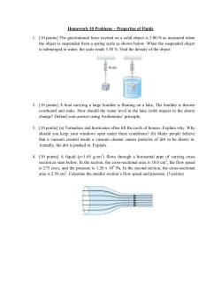

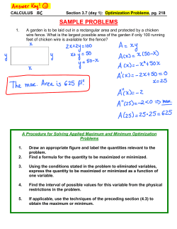
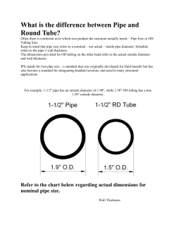
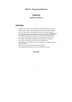

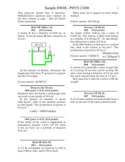


© Copyright 2026