1. No category

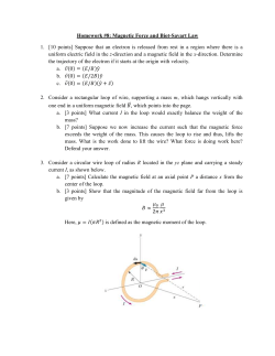
Bennet, E. D., Potts, H. E., Teodoro, L. F.A., and Diver, D. A. (2014) Electron
acceleration by magnetic collapse during decoupling. Monthly Notices of the
Royal Astronomical Society, 445 (2). pp. 1521-1525. ISSN 0035-8711
Copyright © 2014 The Authors
http://eprints.gla.ac.uk/96917
Deposited on: 18 November 2014
Enlighten – Research publications by members of the University of Glasgow
http://eprints.gla.ac.uk
MNRAS 445, 1521–1525 (2014)
doi:10.1093/mnras/stu1857
Electron acceleration by magnetic collapse during decoupling
Euan D. Bennet,1‹ Hugh E. Potts,1 Luis F. A. Teodoro2 and Declan A. Diver1
1 SUPA,
2 BAER
School of Physics and Astronomy, University of Glasgow, Glasgow G12 8QQ, UK
Institute, NASA Ames Research Center, MS 245-3, Moffett Field, CA 94935-1000, USA
Accepted 2014 September 7. Received 2014 August 22; in original form 2013 November 12
ABSTRACT
Key words: magnetic fields – cosmology: theory.
1 I N T RO D U C T I O N
In this paper, a theoretical model first developed by Diver & Teodoro
(2008) will be expanded. Here we will develop a numerical model
used to simulate the motion of charged particles accelerated by the
transient electric and magnetic fields induced in a rapidly evolving
magnetized plasma.
For some years now, it has been proposed that the early Universe
contained large-scale coherent magnetic fields before the recombination era (Kandus, Kunze & Tsagas 2011; Ryu et al. 2012; Widrow
et al. 2012). If this was indeed the case, then the field must have
been pseudo-stochastically arranged over very large length-scales,
such that the total field summed to zero (Moffatt 1978; Ichiki et al.
2006; Durrer 2007). This assumption preserves the cosmological
principles of isotropy and homogeneity. Therefore, it is reasonable
to assume that if large-scale magnetic fields did exist at this epoch,
then the Universe was divided into magnetic domains, each of which
contains a spatially coherent magnetic field not necessarily aligned
with neighbouring domains.
Here we define a domain as a cylindrical region of radius 10 Mpc.
Each domain contains a uniform magnetic field that is coherent over
a length-scale far longer than the radius of the domain.
The boundary between domains must have been provided by
conduction currents in the high-conductivity plasma, which would
be perturbed after the start of global recombination as the current
E-mail: [email protected]
densities vanishes. The model presented in this paper will consider
the electromagnetic behaviour within the current-carrying boundary
of one such domain, and examine the consequences that magnetic
collapse holds for the remaining free charges inside that domain.
During recombination, the Universe made the transition from
fully ionized to just 1 part in 105 ionized (Padmanabhan 1993).
This large-scale neutralization must have removed charges from the
entire plasma, including the current-carrying parts. During such a
transition, the displacement current would assert itself to restore the
balance and sustain the magnetic field structure. The time-varying
electric field of the displacement current would accelerate any remaining free charges in the plasma within a certain locus of the
original conduction current density. This is a direct physical consequence of the large-scale neutralization of an inhomogeneously
magnetized plasma. In the early Universe, the resulting small population of energetic charges has a very small cross-section for recombination due to their high kinetic energy. This means that many
of the charges will persist as a non-equilibrium population.
This idea was developed by Diver & Teodoro (2008) and also by
Teodoro, Diver & Hendry (2008) where they posed the question:
What is the correct physical model that encompasses the critical
physics? The paper constructed the model by identifying the appropriate time-scales that have to be considered. In order to accurately
model the physics of this epoch, the crucial, shortest time-scale
is that of electromagnetic changes communicated at the speed of
light. In other words, the time is right for standard magnetohydrodynamic (MHD) plasma cosmological models (Durrer, Kahniashvili & Yates 1998; Subramanian & Barrow 1998a,b; Jedamzik,
C The Authors 2014. Published by Oxford University Press on behalf of The Royal Astronomical Society. This is an Open Access article distributed under
the terms of the Creative Commons Attribution License (http://creativecommons.org/licenses/by/4.0/), which permits unrestricted reuse, distribution, and
reproduction in any medium, provided the original work is properly cited.
Downloaded from http://mnras.oxfordjournals.org/ at Periodicals Dept on November 18, 2014
This paper identifies the non-equilibrium evolution of magnetic field structures at the onset
of large-scale recombination of an inhomogeneously ionized plasma. The context for this is
the Universe during the epoch of recombination. The electromagnetic treatment of this phase
transition can produce energetic electrons scattered throughout the Universe, localized near the
edges of magnetic domains. This is confirmed by a numerical simulation in which a magnetic
domain is modelled as a uniform field region produced by a thin surrounding current sheet.
Conduction currents sustaining the magnetic structure are removed as the charges comprising
them combine into neutrals. The induced electric field accompanying the magnetic collapse
is able to accelerate ambient stationary electrons (that is, electrons not participating in the
current sheet) to energies of up to order 10keV. This is consistent with theoretical predictions.
The localized electron acceleration leads to local imbalances of charge which has implications
for charge separation in the early Universe.
1522
E. D. Bennet et al.
Katalini´c & Olinto 2000) to be extended. It was concluded that the
only model that takes account of the appropriate physics time-scales
is a fully electromagnetic one.
2 THEORETICAL MODEL
3 E L E C T RO M AG N E T I C E VO L U T I O N
Consider an infinite solenoid (Fig. 1) with the axis pointing in the
axial (z-)direction of a cylindrical polar coordinate system. The current density J is entirely confined to a narrow band in the azimuthal
(φ-)direction. Accordingly, the magnetic field sustained by the conduction current is uniform in the axial direction inside the solenoid,
and zero everywhere outside it. This geometry means that when the
current density decreases with time, the resultant-induced electric
field is azimuthal only, and the induced magnetic perturbation is
confined to the z-direction.
To derive the equation describing the electric field evolution,
begin with Faraday’s law and the complete form of Ampere’s law:
∂B
(1)
∇×E =−
∂t
1 ∂E
,
(2)
∇ × B = μ0 J + 2
c ∂t
ˆ φ is the electric field, B = zˆ Bz is the total magnetic
where E = φE
ˆ φ is the current density, μ0 is the permeability of free
field, J = φJ
space and c is the speed of light in vacuum. In a normal cosmological
model, the scale factor a(t) would be present in equations (1) and (2):
however, since our model describes only the relatively short epoch
of recombination, it is reasonable to consider a(t) to be constant, as
a first approximation.
ˆ zˆ ), taking the
Recasting in cylindrical polar coordinates (ˆr , φ,
curl of equation (1) and the time-derivative of equation (2), and
combining to eliminate Bz , a second-order hyperbolic differential
equation in Eφ emerges:
1 ∂2 Eφ
∂Jφ
∂2 Eφ
1 ∂Eφ
1
−
−
+ 2 Eφ = −μ0
.
(3)
2
2
c ∂t
∂r 2
r ∂r
r
∂t
The main variables and derivatives can be substituted as follows.
In each case the quantity with subscript 0 is the dimensional part, and
the Greek letter is the dimensionless variable to cast the equations
in:
MNRAS 445, 1521–1525 (2014)
Figure 1. Diagram of an infinite solenoid. The top picture (a) shows azimuthal current loops of radius ro carrying current density J in the φdirection only, resulting in a uniform magnetic field B aligned along the
z-direction inside the coil. For clarity, picture (b) shows the same solenoid
from the perspective along the z-axis in the antiparallel direction to the
magnetic field.
r = r0 ρ
(4)
t = t0 τ
(5)
∂
1 ∂
=
∂r
r0 ∂ρ
1 ∂
∂
=
.
∂t
t0 ∂τ
(6)
(7)
Now, recognizing that if the current density is constant then there
will be no electric field, the variables are separable as follows:
Jφ (ρ, τ ) = J0 f (ρ)T (τ )
(8)
Eφ (ρ, τ ) = E0 g(ρ)∂τ T (τ )
(9)
Bz (ρ, τ ) = B0 h(ρ)T (τ ),
(10)
where f(ρ) and T(τ ) are dimensionless functions representing the
spatial form and temporal form of the current density, respectively.
These are specified according to the physical problem studied. The
spatial forms of the electric and magnetic fields are g(ρ) and h(ρ),
respectively, and are to be solved for.
The simplest form of f(ρ) that can be chosen is f(ρ) = δ(ρ − ρ j ),
i.e. a Dirac delta function centred on ρ = ρ j , where ρ j is the radius
Downloaded from http://mnras.oxfordjournals.org/ at Periodicals Dept on November 18, 2014
Magnetic domains as defined in Section 1 are assumed to be sustained by an azimuthal current density caused by the differential
drift of the plasma species in the domain boundary; the resulting
magnetic field is assumed coherent over a scalelength greater than
the radius of the domain. This must be true since in order to refract
the coherent magnetic field, i.e. to change the direction of it at the
boundary between two domains, there must either be a material
change or a current density located at the boundary. In the cosmological context, the latter case must be true. Furthermore, the current
density located at the boundary of a domain sustains the coherent
magnetic field within it.
Consider one such single magnetic domain, the field in which we
shall approximate simply as that arising from an infinite solenoid.
Diver & Teodoro (2008) predicted that electrons in such a domain
could reach energies of ∼7 keV when accelerated by the magnetic
collapse induced by the local domain recombining. Here we will test
their predictions, and the model will be expanded and generalized
such that more complex systems and arrangements of magnetic field
can be studied.
Electron acceleration during decoupling
0.6
0.2
0.3
0.1
0
where in the usual fashion a ∂ symbol denotes a derivative, with the
subscript indicating the independent variable. Now assume that
where κ is a constant. This gives the form of T(τ ) as
and if β is defined as
r0 κ
,
β=
ct0
then equation (11) now becomes
1
∂ρ g(ρ)
μ0 r0 2 J0
2
+
β
f (ρ).
∂ρρ g(ρ) +
g(ρ)
=
−
ρ
ρ2
t0 E0
(13)
μ0 r0 2 J0
κρj K1 (βρj )I1 (βρ) exp (−κτ ).
ct0 E0
1
0
0.3
0.1
0
0
0.2
0.9
0.3
0.6
0.2
0.3
0.1
0
0.2
0.4
0.6
(16)
Combining equations (1) and (16), the magnetic field evolution
can be shown to be
r0 μ0 J0
Bz (ρ, τ ) = B0 exp (−κτ )
B0
2
β r0 μ0 J0
+
ρj K1 (βρj )I0 (βρ) .
(17)
B0
0.8
1
0
0.9
0.3
0.6
0.2
0.3
0.1
0
0
0.2
Each of the six plots in Fig. 2 show a snapshot in time evolution,
beginning with the instant an exponential current density decay
was first imposed. The blue axes and lines show the magnitude of
the z-magnetic field, while the red axes and lines display the total
magnitude (i.e. in the φ-direction) of the electric field.
4 R E S U LT S
If the initial value of the background magnetic field, sustained by
the current density of the azimuthally drifting plasma, is chosen to
be the upper limit of B0 ∼ 10−12 T (Barrow, Ferreira & Silk 1997;
Jedamzik et al. 2000; Chen et al. 2004; Yamazaki, Ichiki, Kajino &
Mathews 2010; Yamazaki et al. 2012), then the electron cyclotron
period informs the characteristic time-scale t0 ∼ 5 s. The typical
length-scale of the magnetic domain radius can be identified as the
Larmor radius for the electrons, here we consider a characteristic
length-scale of 5 × 108 m. These length and time-scales combine
to give a characteristic speed scale of the order of 108 m s−1 .
Fig. 3 shows results for simulations which can be interpreted as a
system with these scalelengths. The simulation was carried out for
100 electrons, evenly spaced throughout the domain from the centre
of the solenoid to just short of the location of the current density.
In the plot, the points show the mean final electron velocity (i.e.
the gyro motion is averaged out over 10 or so cycles leaving only
0.9
0.3
0.6
0.2
0.3
0.1
0.4
0.6
0.4
0.6
0.8
1
0
Time = 100
0.4
0.2
0
radius/arbitrary units
1.2
0
1
0.4
radius/arbitrary units
0
0.8
1.2
Time = 80
(15)
0.6
Time = 60
0.4
0
0.4
radius/arbitrary units
1.2
(14)
Applying the boundary conditions of the solenoid, the electric
field can be expressed fully as
Eφ (ρ, τ ) =
0.8
0.2
0.8
radius/arbitrary units
1
0
1.2
0.4
0.9
0.3
0.6
0.2
0.3
0.1
0
0
0.2
0.4
0.6
0.8
1
0
radius/arbitrary units
Figure 2. Snapshots of the magnitude of magnetic field (blue lines and
axes) and electric field (red lines and axes) as a function of radius inside
an infinite solenoid representing a single magnetic domain. Radius = 1
corresponds to the conduction current-carrying part of the solenoid. The
conduction current density in the solenoid decreases exponentially with
time, with the decrease beginning at the instant time = 0 as shown in
the top-left plot. Subsequent plots show snapshots as time advances. The
magnetic field remains approximately uniform as it decays along with the
current that sustained it.
the drift component of motion) while the lines denote the deviation
from the mean. The usual standard deviation formula was used
to calculate this. Large lines indicate that the gyro motion is still
significant, while small lines show that the drift motion completely
dominates.
The final mean kinetic energy of electrons spaced throughout the
domain ranges up to ∼9 keV for those nearest the domain edge. In
the context that the ‘thermal’ energy is around 0.3 eV, a possible
increase in kinetic energy of four orders of magnitude above the
background means that even a tiny proportion of these energetic
electrons could have an effect in the post-decoupling Universe.
Figs 4 and 5 show the full position and velocity space data for
two individual electrons after they have been accelerated, at opposite extremes of the domain. Note that the magnitudes of velocity
are different by nearly two orders of magnitude. The cyclotron frequency is almost identical for both because the large-scale magnetic
field is approximately uniform for both over the timesteps shown.
However, the electric field is very different because it falls in magnitude with time and distance as it sweeps into the domain from the
edge (i.e. from radius = 1 in the figures), hence the large difference
in drift speed.
MNRAS 445, 1521–1525 (2014)
Downloaded from http://mnras.oxfordjournals.org/ at Periodicals Dept on November 18, 2014
T (τ ) = exp[(−κτ )],
0.6
0.6
Time = 40
magnetic field/arbitrary units
(12)
0.4
0.3
radius/arbitrary units
magnetic field/arbitrary units
∂τ τ τ T (τ )
= κ 2,
∂τ T
0.2
0.9
electric field/arbitrary units
0
0.4
electric field/arbitrary units
0.3
1.2
electric field/arbitrary units
(11)
0.9
electric field/arbitrary units
magnetic field/arbitrary units
r0 2 1
μ0 r02 J0
g(ρ)∂τ τ τ T (τ ) =
f (ρ)∂τ T (τ ),
2
2
t0 c
t0 E0
Time = 20
0.4
electric field/arbitrary units
magnetic field/arbitrary units
−
1
1
∂ρ g(ρ)∂τ T (τ ) − 2 g(ρ)∂τ T (τ )
ρ
ρ
Time = 0
1.2
electric field/arbitrary units
magnetic field/arbitrary units
∂ρρ g(ρ) + ∂τ T (τ ) +
Collapsing Magnetic Field and Induced Electric Field
magnetic field/arbitrary units
of the solenoid. The simplest form of T(τ ) is an exponential decay.
J0 , E0 and B0 are the dimensional parts of the current density and
fields.
Substituting equations (4)–(10) into equation (3) and simplifying:
1523
1524
E. D. Bennet et al.
Mean final kinetic energy of 100 electrons
Post−acceleration trajectory of electron 95
9.03
9.026
9.024
0
400
600
0.1
0.2
0.3
0.4
0.5
0.6
0.7
0.8
0.9
Post−acceleration trajectory of electron 3
2851
2850.5
2850
0
200
400
600
800
1000
time/code units
electron y position with time
0.2
0
−0.2
0
200
400
600
800
1000
time/code units
electron position space
0.02
0
−0.02
−0.04
2850
2850.5
2851
2851.5
x pos/code units
y vel/code units y vel/code units x vel/code units
y pos/code units y pos/code units x pos/code units
Figure 3. Each point denotes the final kinetic energy in keV of a typical
electron after acceleration by the transient electric field caused by the current
collapse. The motion has been averaged over 10 cyclotron periods. The
electrons were initially stationary, and evenly spaced along the radius of the
cylindrical magnetic domain. The x-axis denotes radial distance from the
centre of the magnetic domain, with x = 0 the centre axis and x = 1 as the
location of the current-carrying region. The transient electric field caused
by magnetic collapse propagates into the domain from x = 1. The error bars
accompanying each point essentially show the gyro motion of each electron,
calculated by standard deviation from the mean kinetic energy. Large error
bars indicate that the gyro motion is still significant, while smaller ones
show that the drift motion completely dominates.
2851.5
electron x velocity with time
0.1
0
−0.1
0
200
400
600
800
1000
time/code units
electron y velocity with time
−1
0
1
0
−1
−2
0
200
400
600
800
1000
0
−0.5
9.027
9.028
9.029
9.03
600
800
1000
1
0
−0.5
−1
0
200
400
600
800
1000
time/code units
electron velocity space
0.5
9.026
400
0.5
time/code units
electron position space
−1
9.025
200
time/code units
electron y velocity with time
9.031
4
x 10
1
0.5
0
−0.5
−1
−1
−0.5
0
0.5
1
x vel/code units
Figure 5. The post-acceleration behaviour of a typical single free electron
at starting radius 0.95 in Fig. 3. This plot shows the full position and velocity
space of the electron. The position and velocity coordinates are in code units,
which are related to the characteristic scalelengths described in the text of
Section 4. Note that there are 105 code units in one magnetic domain radius
as depicted in Figs 1–3. Note also the difference in velocity magnitude
between this plot and Fig. 4: this is because the transient electric field falls
in magnitude with time and distance as it sweeps across the domain, leading
to less acceleration further from the domain edge.
of energetic electrons (and associated energetic ions) in the postrecombination Universe. The implications of this include charge
separation and therefore localized non-zero electrostatic potential
which could contribute to structure formation.
Any large-scale magnetic structure in the early Universe must
have been stochastically arranged in domains, in order to preserve
the cosmological principle of anisotropy. The magnetic field within
each domain must itself have been sustained by a conduction current
around the outer edges.
In this paper, we have shown that within one such domain, the
following sequence of events must occur during the epoch of recombination.
0.1
0
−0.1
0
200
400
600
800
1000
time/code units
electron velocity space
0.1
0
−0.1
−0.1
−0.05
0
0.05
0.1
x vel/code units
Figure 4. The post-acceleration behaviour of a typical single free electron
at starting radius 0.03 in Fig. 3. This plot shows the full position and velocity
space. The position and velocity coordinates are in code units, which are
related to the characteristic scalelengths described in the text of Section 4.
Note that there are 105 code units in one magnetic domain radius as depicted
in Figs 1–3.
5 DISCUSSION
If one assumes that the Universe was magnetized pre-decoupling,
then regardless of how the magnetic fields were first induced there
are electromagnetic consequences during the epoch of decoupling.
One of these consequences is the presence of an enduring population
MNRAS 445, 1521–1525 (2014)
0
−0.5
1
Electron starting radius/domain radius
electron x position with time
0.5
(i) Electrons and ions recombine into neutrals throughout the
domain, including in the narrow current-carrying region.
(ii) Recombination causes the current density to collapse as
charge carriers are removed.
(iii) The changing conduction current forces changes in the magnetic field.
(iv) By Maxwell’s equations, the magnetic fluctuation produces
a radiating electromagnetic impulse.
(v) Free charges in the domain encountering that electromagnetic
pulse can be accelerated to energies of up to 9 keV.
(vi) The difference in mobility between accelerated electrons and
ions may result in charge separation if the energy gained is not just
from moving at the drift speed.
For physical scalelengths consistent with much of the literature,
the orders of magnitude of kinetic energy gained by the electrons in
these simulations are consistent with those predicted by the simple
drift speed calculation in Diver & Teodoro (2008). The simulations
show electrons could be accelerated up to ∼10 keV, compared with
a thermal energy of ∼0.3 eV. Once the electrons are accelerated to
such energies, their collisional cross-section is tiny and so generally
the accelerated electrons would carry on uninterrupted into the otherwise cool, dark Universe. The agreement of the results from this
Downloaded from http://mnras.oxfordjournals.org/ at Periodicals Dept on November 18, 2014
0
1000
2
x pos/code units
0
800
y vel/code units
y pos/code units
200
1
time/code units
electron y position with time
4
2
electron x velocity with time
9.028
8
6
electron x position with time
x vel/code units
10
x 10
y vel/code units
x pos/code units
4
9.032
y pos/code units
final mean kinetic energy/keV
12
Electron acceleration during decoupling
1525
simple computational model with the earlier prediction motivates
the development of a more detailed model, for example one that
models the current-carrying region to higher resolution. One might
also consider the signal emitted from the accelerated electrons –
which would be redshifted into the UV today.
The modelling approximations allow scope to try out alternative
models for the progress of global neutralization, for example a
propagating neutralization front travelling at the sound speed, or a
spotty domain with localized hotspots of neutralization that spread
outwards until the domain is fully neutral.
Since the magnetic energy density varies with the square of the
field intensity, lower magnetic field magnitudes in the domains result in lower energies gained by accelerated electrons; in an extreme
lower limit (such as the 10−22 T in Ichiki et al. 2006), the magnetic
energy contribution may be lost in the thermal noise.
tion fraction after recombination was fi = 10−5 . The final factor of
is the fraction of electrons fd within the current-carrying region
which gain a velocity over and above the drift speed. We now have
5.1 The impact on structure formation
AC K N OW L E D G E M E N T S
Diver & Teodoro (2008) constructed their model with the simplifying assumption that the E × B drift was uniform. This cannot by
itself lead to charge separation. We have shown in this article that
the electric field is transient in both space and time, meaning electrons are non-uniformly accelerated to higher energies than simply
acquiring the drift speed. This more sophisticated model permits
the possibility of charge separation. We can estimate the magnitude
of this as follows.
Assume a fraction of unbalanced charge develops as a result
of this charge separation. Comparing the self-electrostatic potential
of the domain with the self-gravitational potential, we see that
EDB gratefully acknowledges support from a University of Glasgow scholarship. Additionally, the authors would like to recognize
support from STFC via grant number ST/I001808/1. The authors
are grateful to the referee for constructive comments which helped
to improve the clarity of the paper.
=
2 e2
.
4π0 Gm2p
(18)
E
Note that is independent of separation length-scale R. SubstiG
E
tuting all of the physical constants, we find = 1.24 × 1036 2 .
G
The ratio will be of order unity if
≥ 10−18 .
(19)
To put this in context, consider the fraction of electrons in a single
magnetic domain that are most affected by the magnetic collapse:
those electrons participating in the current density sustaining the
magnetic field. Recall that in Section 1, the magnetic domains were
of the order of 10 Mpc across. The current-carrying region at a
boundary between two adjacent domains, by contrast, is a cylinder
of the order of 10 pc in diameter. Since the current-carrying region
forms the boundary between two domains it would have length of
the order of 10 Mpc.
Therefore post-recombination, electrons that were originally located in the current-carrying region represent a fraction fe = 10−12
of all electrons in the magnetic domain. Recall also that the ioniza-
(20)
The electrostatic potential from charge separation will be of similar magnitude to the self-gravitational potential of the magnetic
domain if fd ≥ 0.1, i.e. if just 10 per cent of electrons in the currentcarrying region are accelerated to speed faster than the drift speed.
In a region with no dark matter, this electrostatic residual from the
decay of pre-existing magnetic field could nudge the matter towards
gravitational collapse. Observed today however, in the absence of
magnetic fields, the gravitational collapse would be assumed to have
been caused by a density perturbation but in fact would trace out
primordial magnetic field lines.
REFERENCES
Barrow J. D., Ferreira P. G., Silk J., 1997, Phys. Rev. Lett., 78, 3610
Chen G., Mukherjee P., Kahniashvili T., Ratra B., Wang Y., 2004, ApJ, 611,
655
Diver D. A., Teodoro L. F. A., 2008, MNRAS, 385, L73
Durrer R., 2007, New Astron. Rev., 51, 275
Durrer R., Kahniashvili T., Yates A., 1998, Phys. Rev. D, 58, 123004
Ichiki K., Takahashi K., Ohno H., Hanayama H., Sugiyama N., 2006, Science, 311, 827
Jedamzik K., Katalini´c V., Olinto A. V., 2000, Phys. Rev. Lett., 85, 700
Kandus A., Kunze K. E., Tsagas C. G., 2011, Phys. Rep., 505, 1
Moffatt H. K., 1978, Magnetic Field Generation in Electrically Conducting
Fluids. Cambridge Univ. Press, Cambridge
Padmanabhan T., 1993, Structure Formation in the Universe. Cambridge
Univ. Press, Cambridge
Ryu D., Schleicher D. R. G., Treumann R. A., Tsagas C. G., Widrow L. M.,
2012, Space Sci. Rev., 166, 1
Subramanian K., Barrow J. D., 1998a, Phys. Rev. D, 58, 083502
Subramanian K., Barrow J. D., 1998b, Phys. Rev. Lett., 81, 3575
Teodoro L. F. A., Diver D. A., Hendry M. A., 2008, MNRAS, 383, L35
Widrow L. M., Ryu D., Schleicher D. R. G., Subramanian K., Tsagas C. G.,
Treumann R. A., 2012, Space Sci. Rev., 166, 37
Yamazaki D. G., Ichiki K., Kajino T., Mathews G. J., 2010, Phys. Rev. D,
81, 023008
Yamazaki D. G., Kajino T., Mathews G. J., Ichiki K., 2012, Phys. Rep., 517,
141
This paper has been typeset from a TEX/LATEX file prepared by the author.
MNRAS 445, 1521–1525 (2014)
Downloaded from http://mnras.oxfordjournals.org/ at Periodicals Dept on November 18, 2014
2 n2 e 2 R
E
=
G
4π0 R Gn2 m2p
= fe fi fd = 10−17 fd .