1. No category

Modern Optimization Techniques for Big Data
Machine Learning
Tong Zhang
Rutgers University & Baidu Inc.
T. Zhang
Big Data Optimization
1 / 41
Outline
Background:
big data optimization in machine learning: special structure
T. Zhang
Big Data Optimization
2 / 41
Outline
Background:
big data optimization in machine learning: special structure
Single machine optimization
stochastic gradient (1st order) versus batch gradient: pros and cons
algorithm 1: SVRG (Stochastic variance reduced gradient)
algorithm 2: SDCA (Stochastic Dual Coordinate Ascent)
algorithm 3: accelerated SDCA (with Nesterov acceleration)
T. Zhang
Big Data Optimization
2 / 41
Outline
Background:
big data optimization in machine learning: special structure
Single machine optimization
stochastic gradient (1st order) versus batch gradient: pros and cons
algorithm 1: SVRG (Stochastic variance reduced gradient)
algorithm 2: SDCA (Stochastic Dual Coordinate Ascent)
algorithm 3: accelerated SDCA (with Nesterov acceleration)
Distributed optimization
algorithm 4: Minibatch SDCA
algorithm 5: DANE (Distributed Approximate NEwton-type method)
behaves like 2nd order stochastic sampling
other methods
T. Zhang
Big Data Optimization
2 / 41
Mathematical Problem
Big Data Optimization Problem in machine learning:
n
min f (w)
w
f (w) =
1X
fi (w)
n
i=1
Special structure: sum over data: large n
T. Zhang
Big Data Optimization
3 / 41
Mathematical Problem
Big Data Optimization Problem in machine learning:
n
min f (w)
w
f (w) =
1X
fi (w)
n
i=1
Special structure: sum over data: large n
Assumptions on loss function
λ-strong convexity:
λ
f (w 0 ) ≥ f (w) + ∇f (w)> (w 0 − w) + kw 0 − wk22
2
|
{z
}
quadratic lower bound
L-smoothness:
L
fi (w 0 ) ≤ fi (w) + ∇fi (w)> (w 0 − w) + kw 0 − wk22
2
|
{z
}
quadratic upper bound
T. Zhang
Big Data Optimization
3 / 41
Example: Computational Advertising
Large scale regularized logistic regression

min
w
1
n

n
X


ln(1 + e−w > xi yi ) + λ kwk2 
2


2
{z
}
i=1 |
fi (w)
data (xi , yi ) with yi ∈ {±1}
parameter vector w.
λ strongly convex and L = 0.25 maxi kxi k22 + λ smooth.
T. Zhang
Big Data Optimization
4 / 41
Example: Computational Advertising
Large scale regularized logistic regression

min
w
1
n

n
X


ln(1 + e−w > xi yi ) + λ kwk2 
2


2
{z
}
i=1 |
fi (w)
data (xi , yi ) with yi ∈ {±1}
parameter vector w.
λ strongly convex and L = 0.25 maxi kxi k22 + λ smooth.
big data: n ∼ 10 − 100 billion
high dimension: dim(xi ) ∼ 10 − 100 billion
T. Zhang
Big Data Optimization
4 / 41
Example: Computational Advertising
Large scale regularized logistic regression

min
w
1
n

n
X


ln(1 + e−w > xi yi ) + λ kwk2 
2


2
{z
}
i=1 |
fi (w)
data (xi , yi ) with yi ∈ {±1}
parameter vector w.
λ strongly convex and L = 0.25 maxi kxi k22 + λ smooth.
big data: n ∼ 10 − 100 billion
high dimension: dim(xi ) ∼ 10 − 100 billion
How to solve big optimization problems efficiently?
T. Zhang
Big Data Optimization
4 / 41
Optimization Problem: Communication Complexity
From simple to complex
Single machine single-core
can employ sequential algorithms
T. Zhang
Big Data Optimization
5 / 41
Optimization Problem: Communication Complexity
From simple to complex
Single machine single-core
can employ sequential algorithms
Single machine multi-core
relatively cheap communication
T. Zhang
Big Data Optimization
5 / 41
Optimization Problem: Communication Complexity
From simple to complex
Single machine single-core
can employ sequential algorithms
Single machine multi-core
relatively cheap communication
Multi-machine (synchronous)
expensive communication
T. Zhang
Big Data Optimization
5 / 41
Optimization Problem: Communication Complexity
From simple to complex
Single machine single-core
can employ sequential algorithms
Single machine multi-core
relatively cheap communication
Multi-machine (synchronous)
expensive communication
Multi-machine (asynchronous)
break synchronization to reduce communication
T. Zhang
Big Data Optimization
5 / 41
Optimization Problem: Communication Complexity
From simple to complex
Single machine single-core
can employ sequential algorithms
Single machine multi-core
relatively cheap communication
Multi-machine (synchronous)
expensive communication
Multi-machine (asynchronous)
break synchronization to reduce communication
We want to solve simple problem well first, then more complex ones.
T. Zhang
Big Data Optimization
5 / 41
Outline
Background:
big data optimization in machine learning: special structure
Single machine optimization
stochastic gradient (1st order) versus batch gradient: pros and cons
algorithm 1: SVRG (Stochastic variance reduced gradient)
algorithm 2: SDCA (Stochastic Dual Coordinate Ascent)
algorithm 3: accelerated SDCA (with Nesterov acceleration)
Distributed optimization
algorithm 4: Minibatch SDCA
algorithm 5: DANE (Distributed Approximate NEwton-type method)
behaves like 2nd order stochastic sampling
other methods
T. Zhang
Big Data Optimization
6 / 41
Batch Optimization Method: Gradient Descent
Solve
n
w∗ = arg min f (w)
w
f (w) =
1X
fi (w).
n
i=1
Gradient Descent (GD):
wk = wk −1 − ηk ∇f (wk −1 ).
How fast does this method converge to the optimal solution?
T. Zhang
Big Data Optimization
7 / 41
Batch Optimization Method: Gradient Descent
Solve
n
w∗ = arg min f (w)
w
f (w) =
1X
fi (w).
n
i=1
Gradient Descent (GD):
wk = wk −1 − ηk ∇f (wk −1 ).
How fast does this method converge to the optimal solution?
Convergence rate depends on conditions of f (·).
For λ-strongly convex and L-smooth problems, it is linear rate:
f (wk ) − f (w∗ ) = O((1 − ρ)k ),
where ρ = O(λ/L) is the inverse condition number
T. Zhang
Big Data Optimization
7 / 41
Stochastic Approximate Gradient Computation
If
n
1X
fi (w),
f (w) =
n
i=1
GD requires the computation of full gradient, which is extremely costly
n
1X
∇f (w) =
∇fi (w)
n
i=1
T. Zhang
Big Data Optimization
8 / 41
Stochastic Approximate Gradient Computation
If
n
1X
fi (w),
f (w) =
n
i=1
GD requires the computation of full gradient, which is extremely costly
n
1X
∇f (w) =
∇fi (w)
n
i=1
Idea: stochastic optimization employs random sample (mini-batch) B
to approximate
∇f (w) ≈
1 X
∇fi (w)
|B|
i∈B
It is an unbiased estimator
more efficient computation but introduces variance
T. Zhang
Big Data Optimization
8 / 41
SGD versus GD
SGD:
faster computation per step
Sublinear convergence: due to the variance of gradient
˜
approximation. f (wt ) − f (w∗ ) = O(1/t).
GD:
slower computation per step
Linear convergence: f (wt ) − f (w∗ ) = O((1 − ρ)t ).
T. Zhang
Big Data Optimization
9 / 41
SGD versus GD
SGD:
faster computation per step
Sublinear convergence: due to the variance of gradient
˜
approximation. f (wt ) − f (w∗ ) = O(1/t).
GD:
slower computation per step
Linear convergence: f (wt ) − f (w∗ ) = O((1 − ρ)t ).
Improve SGD via variance reduction:
SGD: unbiased statistical estimator of gradient with large variance.
Smaller variance implies faster convergence
Idea: design other unbiased gradient estimators with small variance
T. Zhang
Big Data Optimization
9 / 41
Improving SGD using Variance Reduction
The idea leads to modern stochastic algorithms for big data machine
learning with fast convergence rate
T. Zhang
Big Data Optimization
10 / 41
Improving SGD using Variance Reduction
The idea leads to modern stochastic algorithms for big data machine
learning with fast convergence rate
Collins et al (2008): For special problems, with a relatively
complicated algorithm (Exponentiated Gradient on dual)
Le Roux, Schmidt, Bach (NIPS 2012): A variant of SGD called SAG
(stochastic average gradient)
Johnson and Z (NIPS 2013): SVRG (Stochastic variance reduced
gradient)
Shalev-Schwartz and Z (JMLR 2013): SDCA (Stochastic Dual
Coordinate Ascent)
T. Zhang
Big Data Optimization
10 / 41
Outline
Background:
big data optimization in machine learning: special structure
Single machine optimization
stochastic gradient (1st order) versus batch gradient: pros and cons
algorithm 1: SVRG (Stochastic variance reduced gradient)
algorithm 2: SDCA (Stochastic Dual Coordinate Ascent)
algorithm 3: accelerated SDCA (with Nesterov acceleration)
Distributed optimization
algorithm 4: Minibatch SDCA
algorithm 5: DANE (Distributed Approximate NEwton-type method)
behaves like 2nd order stochastic sampling
other methods
T. Zhang
Big Data Optimization
11 / 41
Stochastic Variance Reduced Gradient: Derivation
Objective function
f (w) =
n
n
i=1
i=1
1X
1 X˜
fi (w) =
fi (w),
n
n
where
˜fi (w) = fi (w) − (∇fi (w)
˜ − ∇f (w))
˜ >w .
{z
}
|
sum to zero
˜ to be an approximate solution (close to w∗ ).
Pick w
T. Zhang
Big Data Optimization
12 / 41
Stochastic Variance Reduced Gradient: Derivation
Objective function
f (w) =
n
n
i=1
i=1
1X
1 X˜
fi (w) =
fi (w),
n
n
where
˜fi (w) = fi (w) − (∇fi (w)
˜ − ∇f (w))
˜ >w .
{z
}
|
sum to zero
˜ to be an approximate solution (close to w∗ ).
Pick w
SVRG rule:
˜ + ∇f (w)]
˜ .
wt = wt−1 − ηt ∇˜fi (wt−1 ) = wt−1 − ηt [∇fi (wt−1 ) − ∇fi (w)
|
{z
}
small variance
Compare to SGD rule:
wt = wt−1 − ηt ∇fi (wt−1 )
| {z }
large variance
T. Zhang
Big Data Optimization
12 / 41
SVRG Algorithm
Procedure SVRG
Parameters update frequency m and learning rate η
˜0
Initialize w
Iterate: for s = 1, 2, . . .
˜ =w
˜ s−1
w
1 Pn
˜
µ
˜ = n i=1 ∇ψi (w)
˜
w0 = w
Iterate: for t = 1, 2, . . . , m
Randomly pick it ∈ {1, . . . , n} and update weight
˜ +µ
wt = wt−1 − η(∇ψit (wt−1 ) − ∇ψit (w)
˜)
end
˜ s = wm
Set w
end
T. Zhang
Big Data Optimization
13 / 41
SVRG v.s. Batch Gradient Descent: fast convergence
Number of examples needed to achieve accuracy:
˜ · L/λ log(1/))
Batch GD: O(n
˜
SVRG: O((n
+ L/λ) log(1/))
Assume L-smooth loss fi and λ strongly convex objective function.
SVRG has fast convergence — condition number effectively reduced
The gain of SVRG over batch algorithm is significant when n is large.
T. Zhang
Big Data Optimization
14 / 41
Outline
Background:
big data optimization in machine learning: special structure
Single machine optimization
stochastic gradient (1st order) versus batch gradient: pros and cons
algorithm 1: SVRG (Stochastic variance reduced gradient)
algorithm 2: SDCA (Stochastic Dual Coordinate Ascent)
algorithm 3: accelerated SDCA (with Nesterov acceleration)
Distributed optimization
algorithm 4: Minibatch SDCA
algorithm 5: DANE (Distributed Approximate NEwton-type method)
behaves like 2nd order stochastic sampling
other methods
T. Zhang
Big Data Optimization
15 / 41
Motivation of SDCA: regularized loss minimization
Assume we want to solve the Lasso problem:
" n
#
1X >
2
min
(w xi − yi ) + λkwk1
w
n
i=1
T. Zhang
Big Data Optimization
16 / 41
Motivation of SDCA: regularized loss minimization
Assume we want to solve the Lasso problem:
" n
#
1X >
2
min
(w xi − yi ) + λkwk1
w
n
i=1
or the ridge regression problem:


 n

1 X >

λ
2
2
min 
(w xi − yi ) +
kwk2 


w
 n i=1
|2 {z } 
|
{z
} regularization
loss
Goal: solve regularized loss minimization problems as fast as we can.
T. Zhang
Big Data Optimization
16 / 41
Motivation of SDCA: regularized loss minimization
Assume we want to solve the Lasso problem:
" n
#
1X >
2
min
(w xi − yi ) + λkwk1
w
n
i=1
or the ridge regression problem:


 n

1 X >

λ
2
2
min 
(w xi − yi ) +
kwk2 


w
 n i=1
|2 {z } 
|
{z
} regularization
loss
Goal: solve regularized loss minimization problems as fast as we can.
solution: proximal Stochastic Dual Coordinate Ascent (Prox-SDCA).
can show: fast convergence of SDCA.
T. Zhang
Big Data Optimization
16 / 41
General Problem
Want to solve:
#
n
1X
φi (Xi> w) + λg(w) ,
min P(w) :=
w
n
"
i=1
where Xi are matrices; g(·) is strongly convex.
Examples:
Multi-class logistic loss
φi (Xi> w) = ln
K
X
exp(w > Xi,` ) − w > Xi,yi .
`=1
L1 − L2 regularization
g(w) =
T. Zhang
1
σ
kwk22 + kwk1
2
λ
Big Data Optimization
17 / 41
Dual Formulation
Primal:
"
#
n
1X
>
min P(w) :=
φi (Xi w) + λg(w) ,
w
n
i=1
Dual:
"
n
n
1 X
Xi αi
λn
1X
−φ∗i (−αi ) − λg ∗
max D(α) :=
α
n
i=1
!#
i=1
with the relationship
w = ∇g
∗
n
1 X
Xi αi
λn
!
.
i=1
The convex conjugate (dual) is defined as φ∗i (a) = supz (az − φi (z)).
SDCA: randomly pick i to optimize D(α) by varying αi while keeping
other dual variables fixed.
T. Zhang
Big Data Optimization
18 / 41
Example: L1 − L2 Regularized Logistic Regression
Primal:
n
P(w) =
1X
λ
>
ln(1 + e−w Xi Yi ) + w > w + σkwk1 .
{z
} |2
|
n
{z
}
i=1
φi (w)
λg(w)
Dual: with αi Yi ∈ [0, 1]
n
D(α) =
1X
λ
−αi Yi ln(αi Yi ) − (1 − αi Yi ) ln(1 − αi Yi ) − ktrunc(v , σ/λ)k22
{z
} 2
|
n
i=1
φ∗i (−αi )
n
s.t. v =
1 X
αi Xi ;
λn
w = trunc(v , σ/λ)
i=1
where


uj − δ
trunc(u, δ)j = 0


uj + δ
T. Zhang
Big Data Optimization
if uj > δ
if |uj | ≤ δ
if uj < −δ
19 / 41
Proximal-SDCA for L1 -L2 Regularization
Algorithm:
P
Keep dual α and v = (λn)−1 i αi Xi
Randomly pick i
Find ∆i by approximately maximizing:
−φ∗i (αi + ∆i ) − trunc(v , σ/λ)> Xi ∆i −
1
kXi k2 2 ∆2i ,
2λn
where φ∗i (αi + ∆) = (αi + ∆)Yi ln((αi + ∆)Yi ) + (1 − (αi + ∆)Yi ) ln(1 − (αi + ∆)Yi )
α = α + ∆ i · ei
v = v + (λn)−1 ∆i · Xi .
Let w = trunc(v , σ/λ).
T. Zhang
Big Data Optimization
20 / 41
Fast Convergence of SDCA
The number of iterations needed to achieve accuracy
For L-smooth loss:
˜
O
n+
L
λ
log
1
For non-smooth but G-Lipschitz loss (bounded gradient):
G2
˜
O n+
λ
T. Zhang
Big Data Optimization
21 / 41
Fast Convergence of SDCA
The number of iterations needed to achieve accuracy
For L-smooth loss:
˜
O
n+
L
λ
log
1
For non-smooth but G-Lipschitz loss (bounded gradient):
G2
˜
O n+
λ
Similar to that of SVRG; and effective when n is large
T. Zhang
Big Data Optimization
21 / 41
Solving L1 with Smooth Loss
Want to solve L1 regularization to accuracy with smooth φi :
n
1X
φi (w) + σkwk1 .
n
i=1
Apply Prox-SDCA with extra term 0.5λkwk22 , where λ = O():
˜ + 1/).
number of iterations needed by prox-SDCA is O(n
T. Zhang
Big Data Optimization
22 / 41
Solving L1 with Smooth Loss
Want to solve L1 regularization to accuracy with smooth φi :
n
1X
φi (w) + σkwk1 .
n
i=1
Apply Prox-SDCA with extra term 0.5λkwk22 , where λ = O():
˜ + 1/).
number of iterations needed by prox-SDCA is O(n
Compare to (number of examples needed to go through):
2 ).
˜
Dual Averaging SGD (Xiao): O(1/
√
˜
FISTA (Nesterov’s batch accelerated proximal gradient): O(n/
).
Prox-SDCA wins in the statistically interesting regime: > Ω(1/n2 )
T. Zhang
Big Data Optimization
22 / 41
Solving L1 with Smooth Loss
Want to solve L1 regularization to accuracy with smooth φi :
n
1X
φi (w) + σkwk1 .
n
i=1
Apply Prox-SDCA with extra term 0.5λkwk22 , where λ = O():
˜ + 1/).
number of iterations needed by prox-SDCA is O(n
Compare to (number of examples needed to go through):
2 ).
˜
Dual Averaging SGD (Xiao): O(1/
√
˜
FISTA (Nesterov’s batch accelerated proximal gradient): O(n/
).
Prox-SDCA wins in the statistically interesting regime: > Ω(1/n2 )
Can design accelerated prox-SDCA always superior to FISTA
T. Zhang
Big Data Optimization
22 / 41
Outline
Background:
big data optimization in machine learning: special structure
Single machine optimization
stochastic gradient (1st order) versus batch gradient: pros and cons
algorithm 1: SVRG (Stochastic variance reduced gradient)
algorithm 2: SDCA (Stochastic Dual Coordinate Ascent)
algorithm 3: accelerated SDCA (with Nesterov acceleration)
Distributed optimization
algorithm 4: Minibatch SDCA
algorithm 5: DANE (Distributed Approximate NEwton-type method)
behaves like 2nd order stochastic sampling
other methods
T. Zhang
Big Data Optimization
23 / 41
Accelerated Prox-SDCA
Solving:
n
P(w) :=
1X
φi (Xi> w) + λg(w)
n
i=1
Convergence rate of Prox-SDCA depends on O(1/λ)
Inferior
√ to acceleration when λ is very small O(1/n), which has
O(1/ λ) dependency
T. Zhang
Big Data Optimization
24 / 41
Accelerated Prox-SDCA
Solving:
n
P(w) :=
1X
φi (Xi> w) + λg(w)
n
i=1
Convergence rate of Prox-SDCA depends on O(1/λ)
Inferior
√ to acceleration when λ is very small O(1/n), which has
O(1/ λ) dependency
Inner-outer Iteration Accelerated Prox-SDCA
Pick a suitable κ = Θ(1/n) and β
For t = 2, 3 . . . (outer iter)
˜t (w) = λg(w) + 0.5κkw − y t−1 k22 (κ-strongly convex)
Let g
˜ t (w) = P(w) − λg(w) + g
˜t (w) (redefine P(·) – κ strongly convex)
Let P
˜ t (w) for (w (t) , α(t) ) with prox-SDCA (inner iter)
Approximately solve P
Let y (t) = w (t) + β(w (t) − w (t−1) ) (acceleration)
T. Zhang
Big Data Optimization
24 / 41
Performance Comparisons
Problem
SVM
Algorithm
SGD
AGD (Nesterov)
Acc-Prox-SDCA
Lasso
SGD and variants
Stochastic Coordinate Descent
FISTA
Acc-Prox-SDCA
SGD, SDCA
Ridge Regression
AGD
Acc-Prox-SDCA
T. Zhang
Big Data Optimization
Runtime
1
λ
q
1
λ q
n
n + min{ λ1 , λ
}
d
2
n
q
n 1
q n + min{ 1 , n }
nq
+ λ1
n λ1
q n + min{ λ1 , λn }
n
25 / 41
Additional Related Work on Acceleration
Methods achieving fast accelerated convergence comparable to
Acc-Prox-SDCA
Qihang Lin, Zhaosong Lu, Lin Xiao, An Accelerated Proximal
Coordinate Gradient Method and its Application to Regularized
Empirical Risk Minimization, 2014, arXiv
Yuchen Zhang, Lin Xiao, Stochastic Primal-Dual Coordinate Method
for Regularized Empirical Risk Minimization, 2014, arXiv
T. Zhang
Big Data Optimization
26 / 41
Distributed Computing: Distribution Schemes
Distribute data (data parallelism)
all machines have the same parameters
each machine has a different set of data
Distribute features (model parallelism)
all machines have the same data
each machine has a different set of parameters
Distribute data and features (data & model parallelism)
each machine has a different set of data
each machine has a different set of parameters
T. Zhang
Big Data Optimization
27 / 41
Main Issues in Distributed Large Scale Learning
System Design and Network Communication
data parallelism: need to transfer a reasonable size chunk of data
each time (mini batch)
model parallelism: distributed parameter vector (parameter server)
T. Zhang
Big Data Optimization
28 / 41
Main Issues in Distributed Large Scale Learning
System Design and Network Communication
data parallelism: need to transfer a reasonable size chunk of data
each time (mini batch)
model parallelism: distributed parameter vector (parameter server)
Model Update Strategy
synchronous
asynchronous
T. Zhang
Big Data Optimization
28 / 41
Outline
Background:
big data optimization in machine learning: special structure
Single machine optimization
stochastic gradient (1st order) versus batch gradient: pros and cons
algorithm 1: SVRG (Stochastic variance reduced gradient)
algorithm 2: SDCA (Stochastic Dual Coordinate Ascent)
algorithm 3: accelerated SDCA (with Nesterov acceleration)
Distributed optimization
algorithm 4: Minibatch SDCA
algorithm 5: DANE (Distributed Approximate NEwton-type method)
behaves like 2nd order stochastic sampling
other methods
T. Zhang
Big Data Optimization
29 / 41
MiniBatch
Vanilla SDCA (or SGD) is difficult to parallelize
Solution: use minibatch (thousands to hundreds of thousands)
T. Zhang
Big Data Optimization
30 / 41
MiniBatch
Vanilla SDCA (or SGD) is difficult to parallelize
Solution: use minibatch (thousands to hundreds of thousands)
Problem: simple minibatch implementation slows down convergence
limited gain for using parallel computing
T. Zhang
Big Data Optimization
30 / 41
MiniBatch
Vanilla SDCA (or SGD) is difficult to parallelize
Solution: use minibatch (thousands to hundreds of thousands)
Problem: simple minibatch implementation slows down convergence
limited gain for using parallel computing
Solution:
use Nesterov acceleration
use second order information (e.g. approximate Newton steps)
T. Zhang
Big Data Optimization
30 / 41
MiniBatch SDCA with Acceleration
Parameters scalars λ, γ and θ ∈ [0, 1] ; mini-batch size b
(0)
(0)
Initialize α1 = · · · = αn = α
¯ (0) = 0, w (0) = 0
Iterate: for t = 1, 2, . . .
u (t−1) = (1 − θ)w (t−1) + θα
¯ (t−1)
Randomly pick subset I ⊂ {1, . . . , n} of size b and update
(t)
(t−1)
αi = (1 − θ)αi
− θ∇fi (u (t−1) )/(λn) for i ∈ I
(t)
(t−1)
αj = αj
for j ∈
/I
P
(t)
(t−1)
(t)
(t−1)
α
¯ =α
¯
+ i∈I (αi − αi
)
w (t) = (1 − θ)w (t−1) + θα
¯ (t)
end
Better than vanilla block SDCA, and allow large batch.
T. Zhang
Big Data Optimization
31 / 41
Example
−1
10
Primal suboptimality
m=52
m=523
m=5229
AGD
SDCA
−2
10
−3
10
6
10
7
10
8
10
#processed examples
MiniBatch SDCA with acceleration can employ large minibatch size.
T. Zhang
Big Data Optimization
32 / 41
Outline
Background:
big data optimization in machine learning: special structure
Single machine optimization
stochastic gradient (1st order) versus batch gradient: pros and cons
algorithm 1: SVRG (Stochastic variance reduced gradient)
algorithm 2: SDCA (Stochastic Dual Coordinate Ascent)
algorithm 3: accelerated SDCA (with Nesterov acceleration)
Distributed optimization
algorithm 4: Minibatch SDCA
algorithm 5: DANE (Distributed Approximate NEwton-type method)
behaves like 2nd order stochastic sampling
other methods
T. Zhang
Big Data Optimization
33 / 41
Communication Efficient Distributed Computing
Assume: data distributed over machines
m processors
each has n/m examples
Simple Computational Strategy — One Shot Averaging (OSA)
run optimization on m machines separately
obtaining parameters w (1) , . . . , w (m)
average the parameters: l
¯ = m−1
w
T. Zhang
Pm
i=1
w (i)
Big Data Optimization
34 / 41
Improvement
OSA Strategy’s advantage:
machines run independently
simple and computationally efficient; asymptotically good in theory
Disadvantage:
practically inferior to training all examples on a single machine
T. Zhang
Big Data Optimization
35 / 41
Improvement
OSA Strategy’s advantage:
machines run independently
simple and computationally efficient; asymptotically good in theory
Disadvantage:
practically inferior to training all examples on a single machine
Traditional solution in optimization: ADMM
New Idea: via 2nd order gradient sampling
Distributed Approximate NEwton (DANE)
T. Zhang
Big Data Optimization
35 / 41
Distribution Scheme
Assume: data distributed over machines with decomposed problem
f (w) =
m
X
f (`) (w).
`=1
m processors
each f (`) (w) has n/m randomly partitioned examples
each machine holds a complete set of parameters
T. Zhang
Big Data Optimization
36 / 41
DANE
˜ using OSA
Starting with w
Iterate
˜ and define
Take w
˜f (`) (w) = f (`) (w) − (∇f (`) (w)
˜ − ∇f (w))
˜ >w
on each machine solves
w (`) = arg min ˜f (`) (w)
w
independently.
˜
Take partial average as the next w
T. Zhang
Big Data Optimization
37 / 41
DANE
˜ using OSA
Starting with w
Iterate
˜ and define
Take w
˜f (`) (w) = f (`) (w) − (∇f (`) (w)
˜ − ∇f (w))
˜ >w
on each machine solves
w (`) = arg min ˜f (`) (w)
w
independently.
˜
Take partial average as the next w
Lead to fast convergence: O((1 − ρ)` ) with ρ ≈ 1
T. Zhang
Big Data Optimization
37 / 41
Reason: Approximate Newton Step
On each machine, we solve:
min ˜f (`) (w).
w
It can be regarded as approximate minimization of


1
 ˜
˜ > ∇2 f (`) (w)(w
˜
˜ 
˜ > (w − w)
˜ +
(w − w)
− w)
min f (w)
+ ∇f (w)
.
w
{z
}
2 |
˜
2nd order gradient sampling from ∇2 f (w)
Approximate Newton Step with sampled approximation of Hessian
T. Zhang
Big Data Optimization
38 / 41
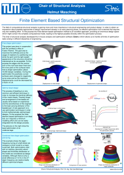
Comparisons
COV1
MNIST−47
ASTRO
0.231
DANE
ADMM
OSA
Opt
0.06
0.07
0.05
0.23
0.06
0.229
0.05
0.04
0.03
0
T. Zhang
5
t
10
0.04
0
5
t
Big Data Optimization
10
0
5
t
10
39 / 41
Summary
Optimization in machine learning: sum over data structure
Traditional methods: gradient based batch algorithms
do not take advantage of special structure
Recent progress: stochastic optimization with fast rate
take advantage of special structure: suitable for single machine
T. Zhang
Big Data Optimization
40 / 41
Summary
Optimization in machine learning: sum over data structure
Traditional methods: gradient based batch algorithms
do not take advantage of special structure
Recent progress: stochastic optimization with fast rate
take advantage of special structure: suitable for single machine
Distributed computing (data parallelism and synchronous update)
minibatch SDCA
DANE (batch algorithm on each machine + synchronization)
T. Zhang
Big Data Optimization
40 / 41
Summary
Optimization in machine learning: sum over data structure
Traditional methods: gradient based batch algorithms
do not take advantage of special structure
Recent progress: stochastic optimization with fast rate
take advantage of special structure: suitable for single machine
Distributed computing (data parallelism and synchronous update)
minibatch SDCA
DANE (batch algorithm on each machine + synchronization)
Other approaches
algorithmic side: ADMM, Asynchronous updates (Hogwild), etc
system side: distributed vector computing (parameter servers) – Baidu
has industrial leading solution
T. Zhang
Big Data Optimization
40 / 41
Summary
Optimization in machine learning: sum over data structure
Traditional methods: gradient based batch algorithms
do not take advantage of special structure
Recent progress: stochastic optimization with fast rate
take advantage of special structure: suitable for single machine
Distributed computing (data parallelism and synchronous update)
minibatch SDCA
DANE (batch algorithm on each machine + synchronization)
Other approaches
algorithmic side: ADMM, Asynchronous updates (Hogwild), etc
system side: distributed vector computing (parameter servers) – Baidu
has industrial leading solution
Fast developing field; many exciting new ideas
T. Zhang
Big Data Optimization
40 / 41
References
Rie Johnson and TZ. Accelerating Stochastic Gradient Descent
using Predictive Variance Reduction, NIPS 2013.
Lin Xiao and TZ. A Proximal Stochastic Gradient Method with
Progressive Variance Reduction, SIAM J. Opt, to appear.
Shai Shalev-Shwartz and TZ. Stochastic Dual Coordinate Ascent
Methods for Regularized Loss Minimization, JMLR 14:567-599,
2013.
Shai Shalev-Shwartz and TZ. Accelerated Proximal Stochastic Dual
Coordinate Ascent for Regularized Loss Minimization, Math
Programming, to appear.
Shai Shalev-Schwartz and TZ. Accelerated Mini-Batch Stochastic
Dual Coordinate Ascent, NIPS 2013.
Ohad Shamir and Nathan Srebro and TZ. Communication-Efficient
Distributed Optimization using an Approximate Newton-type Method,
ICML 2014.
T. Zhang
Big Data Optimization
41 / 41