
Contextual Synonym Dictionary for Visual Object Retrieval Wenbin Tang , Rui Cai
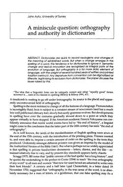
Contextual Synonym Dictionary for Visual Object Retrieval∗
†
Wenbin Tang† ‡§ , Rui Cai† , Zhiwei Li† , and Lei Zhang†
†
Microsoft Research Asia
Dept. of Computer Science and Technology, Tsinghua University
§
Tsinghua National Laboratory for Information Science and Technology
‡
[email protected]
{ruicai, zli, leizhang}@microsoft.com
ABSTRACT
1. INTRODUCTION
In this paper, we study the problem of visual object retrieval
by introducing a dictionary of contextual synonyms to narrow down the semantic gap in visual word quantization. The
basic idea is to expand a visual word in the query image with
its synonyms to boost the retrieval recall. Unlike the existing work such as soft-quantization, which only focuses on the
Euclidean (l2 ) distance in descriptor space, we utilize the visual words which are more likely to describe visual objects
with the same semantic meaning by identifying the words
with similar contextual distributions (i.e. contextual synonyms). We describe the contextual distribution of a visual
word using the statistics of both co-occurrence and spatial
information averaged over all the image patches having this
visual word, and propose an efficient system implementation to construct the contextual synonym dictionary for a
large visual vocabulary. The whole construction process is
unsupervised and the synonym dictionary can be naturally
integrated into a standard bag-of-feature image retrieval system. Experimental results on several benchmark datasets
are quite promising. The contextual synonym dictionarybased expansion consistently outperforms the l2 distancebased soft-quantization, and advances the state-of-the-art
performance remarkably.
To retrieve visual objects from a large-scale image database,
most of the sophisticated methods in this area are based
on the well-known bag-of-feature framework [14, 18], which
typically works as follows. First, for each database image,
local region descriptors such as the Scale Invariant Feature
Transform (SIFT) [10, 20] are extracted. And then the highdimensional local descriptors are quantized into discrete visual words by utilizing a visual vocabulary. The most common method to construct a visual vocabulary is to perform
clustering (e.g. K-means) on the descriptors extracted from a
set of training images; and each cluster is treated as a visual
word described by its center. The quantization step is essentially to assign a local descriptor to its nearest visual word
in the vocabulary in terms of Euclidean (l2 ) distance using
various approximate search algorithms like KD-tree [10, 15],
Locality Sensitive Hashing [3] and Compact Projection [13].
After the quantization, each image is represented by the frequency histogram of a bag of visual words. Taking visual
words as keys, images in the database are indexed by inverted files for quick access and search.
Visual descriptor quantization is a key step to develop a
scalable and fast solution for image retrieval on a large scale
database. However, it also brings two serious and unavoidable problems: mismatch and semantic gap.
Mismatch is due to the polysemy phenomenon, which
means one visual word is too coarse to distinguish descriptors extracted from semantically different objects. This phenomenon is particularly prominent when the visual vocabulary is small. Fig. 1 shows some visual words from a vocabulary with 500K visual words constructed based on the
Oxford Buildings Dataset [15]. The visual words in the first
row are the top-5 nearest neighbors to the query word Q.
Obviously these words describe objects with different semantic meanings (e.g. pillar, fence, wall), but have very close l2
distances to Q. In a smaller visual vocabulary, they are
very likely to be grouped into one word and lead to poor
precision in retrieval. To address this problem, the simplest way to increase the discriminative capability of visual
words is enlarging the vocabulary [15]. Other remarkable
approaches working on this problem include bundling features [25], spatial-bag-of-features [1], hamming embedding
and weak geometry consistency [5, 6], utilizing contextual
dissimilarity measure [7], high-order spatial features [32],
and compositional features [26], etc. In summary, by introducing additional spatial and contextual constraints into
visual word matching, these approaches have made significant improvements on retrieval precision.
Categories and Subject Descriptors
I.2.10 [Vision and Scene Understanding]: Vision
General Terms
Algorithms, Experimentation, Performance
Keywords
Bag-of-word, object retrieval, visual synonym dictionary,
query expansion
∗Area chair: Tat-Seng Chua
†This work was performed at Microsoft Research Asia.
Permission to make digital or hard copies of all or part of this work for
personal or classroom use is granted without fee provided that copies are
not made or distributed for profit or commercial advantage and that copies
bear this notice and the full citation on the first page. To copy otherwise, to
republish, to post on servers or to redistribute to lists, requires prior specific
permission and/or a fee.
MM’11, November 28–December 1, 2011, Scotsdale, Arizona, USA.
Copyright 2011 ACM 978-1-4503-0616-4/11/11 ...$10.00.
503
Q (radius ≈ 150.0)
rank-1 (l2 = 159.9)
rank-2 (l2 = 179.0)
rank-3 (l2 = 181.8)
rank-4 (l2 = 181.9)
rank-5 (l2 = 183.6)
rank-361 (l2 = 264.5) rank-57284 (l2 = 408.8) rank-60561 (l2 = 410.7) rank-209948 (l2 = 463.7) rank-481363 (l2 = 571.3)
Figure 1: An example to illustrate the “semantic gap” between descriptors and semantic objects. Each visual
word is represented by a panel containing 9 patches which are the closest samples to the corresponding
cluster center. The Harris scale of each patch is marked with a red circle. Given the query word Q, its top-5
nearest neighbor words under l2 distance are shown in the first row. The second row lists another 5 visual
words (actually were identified by the algorithm in Section 2) which are more semantically related to the
query word but are far away in the descriptor space. This example was extracted from a 500K vocabulary
constructed based on the Oxford Building Dataset [15].
By contrast, semantic gap leads to the synonymy phenomenon, which means several different visual words actually describe semantically same visual objects. This phenomenon is especially obvious when adopting a large visual vocabulary, and usually results in poor recall performance in visual object retrieval [15]. In Fig. 1, there are
another 5 visual words in the second row which are more semantically related to the query word Q but are far away
from Q in the descriptor space. One of the reasons behind this phenomenon is the poor robustness of local descriptor algorithms. In fact, even those state-of-the-art local descriptors like SIFT are still sensitive to small disturbances (e.g. changes in viewpoint, scale, blur, and capturing condition) and output unstable and noisy feature values [19]. To increase the recall rate, a few research efforts
have been devoted to reducing the troubles caused by synonymous words. One of the most influential techniques is the
query expansion strategy proposed in [2], which completes
the query set using visual words taken from matching objects in the first-round search results. Another method worthy of notice is soft-quantization (or soft-assignment), which
assigns a descriptor to a weighted combination of nearest visual words [16, 21]. Statistical learning methods were also
adopted to bridge semantic gap, e.g., learning a transformation from original descriptor space (e.g. SIFT) to a new
Euclidean space in which l2 distance is more correlated to
semantic divergence [17, 23]. A more direct approach was
proposed in [12] to estimate the semantic coherence of two
visual words via counting the frequency that the two words
match with each other in a training set. A similar technique is also applied in [4], where spatial verifications are
employed between the query and top-ranked images in the
first-round result to detect matching points with different
visual words, then the detected word pairs are viewed as
synonyms and used to update the initial query histogram.
Recently, there is another trend to bridge semantic gap in
visual retrieval. The basic idea is to incorporate textual in-
formation to promote more meaningful visual features [8] or
provide more accurate combinational similarity measure [24,
11]. For example, in [8], auxiliary visual words are identified by propagating the similarity across both visual and
textual graphs. Incorporating textual information in visual
retrieval is a promising research area as surrounding text
is indeed available in many application scenarios (e.g. neardup key-frame retrieval in video search [24]). However, this
is beyond the scope of this paper, in which we still focus on
leveraging pure visual information.
In this paper, we target at providing a simple yet effective
solution to narrow down the semantic gap in visual object
retrieval. In contrast, most aforementioned approaches are
practically expensive. For example, query expansion needs
to do multiple search processes; and its performance highly
depends on the quality of the initial recall [2]. Learningbased methods [12, 17, 23] need to collect a set of matching
point pairs as training data. To construct a comprehensive training set, it usually needs a large image database
and has to run complex geometric verification algorithms
like RANSAC on candidate image pairs to identify possible
matching points. Even so, the obtained training samples
(pairs of synonymous words) are still very sparse when the
vocabulary size is large. Soft-quantization is cheap and effective, but in essence it can only handle the over-splitting
cases in quantization. We argue that the existing l2 distancebased soft-quantization is incapable of dealing with semantic
gap. This is because visual words that are close in l2 distance
do not always have similar semantic meanings, as shown in
Fig. 1.
However, the “expansion” idea behind soft-quantization
and query expansion is very praiseworthy. It reminds us of
the effective synonym expansion strategy in text retrieval [22].
For visual object retrieval, the main challenge here is how to
identify synonyms from a visual vocabulary. In this paper,
we once again borrow the experience from the text domain.
In text analysis, synonyms can be identified by finding words
504
rc × scalepi
sector K
sector 1
sector 1
sector K
pi
…
pj
swpj→pi
Rp
i
sector 2
…
…
…
…
sector 2
rotate
…
(a)
(c)
(b)
Contextual Distribution
of the visual word
(d)
Figure 2: An illustration of the process to estimate the contextual distribution of a visual word ωm . (a)
For each instance pi of the visual word, its visual context is defined as a spatial circular region Rpi with the
radius rc × scalepi ; (b) A point in the visual context is weighted according to its spatial distance to pi ; (c) The
dominant orientation of pi is rotated to be vertical; Rpi is partitioned into K sectors, and for each sector a
sub-histograms is constructed; (d) The sub-histograms of all the instances of the visual word ωm are aggregated
to describe the contextual distribution of ωm .
work usually works on a small vocabulary as the number
of possible combinations increases in exponential order of
the vocabulary size [27, 34]. Moreover, they can leverage
supervised information (e.g. image categories) to learn distance measures between visual phrase (e.g. the Mahalanobis
distance in [29], boosting in [26], and the kernel-based learning in [32]). In retrieval, visual phrase is considered as an
additional kind of feature to provide better image representations. By contrast, the contextual synonym dictionary
in this paper is defined on single visual word. There is no
explicit “phrases” but embeds some implicit contextual relationships among visual words. Our approach can work on
large vocabulary as the cost is just linear with the vocabulary size. For retrieval, the synonym dictionary is utilized
to expand query terms and the image representation is still
a histogram of visual words. Therefore, the contextual synonym dictionary can be naturally integrated into a standard
bag-of-feature image retrieval system.
The rest of the paper is organized as follows. We introduce the visual context and contextual similarity measure
in Section 2. Section 3 describes the system implementation
to construct a contextual synonym dictionary, and presents
how to apply the synonym dictionary to expand visual words
in visual object retrieval. Experimental results are discussed
in Section 4; and conclusion is drawn in Section 5.
with similar contextual distributions [28], where the textual
context refers to the surrounding text of a word. Analogically, we can define the visual context as a set of local points
which are in a certain spatial region of a visual word. Intuitively, visual words representing the same semantic meaning tend to have similar visual contextual distributions. An
evidence to support this assumption is the “visual phrase”
reported in the recent literature of object recognition [27,
34, 26, 30, 29, 33, 32]. A visual phrase is a set of frequently
co-occurring visual words, and has been observed to exist in
visual objects from the same semantic category (e.g. cars).
Besides co-occurrence, we also incorporate local spatial information to the visual contextual distribution as well as
the corresponding contextual similarity measure1 . Next, we
define the “contextual synonyms” of a visual word as its nearest neighbors in terms of the contextual similarity measure.
The ensemble of contextual synonyms of all the visual words
is a contextual synonym dictionary, which can be computed
offline and stored in memory for fast access. For retrieval,
each visual word extracted on the query image is expanded
to a weighted combination of its visual synonyms, then the
expanded histogram is taken as the new query.
As a side-note, here we would like to make a distinction
between the proposed contextual synonym dictionary and
visual phrase in existing work. Actually, their perspectives
are different. To identify visual phrases, the typical process
is to first discover combinations of visual words and then
group these combinations according to some distance measures. Each group is taken as a visual phrase. The related
2. VISUAL CONTEXTUAL SYNONYMS
In this section, we introduce the concepts of visual context
and contextual distribution, as well as how to measure the
contextual similarity of two visual words according to their
contextual distributions.
To make a clear presentation and facilitate the following
discussions, we first define some notations used in this paper.
In the bag-of-feature framework, there is a visual vocabulary
Ω = {ω1 , . . . , ωm , . . . , ωM } in which ωm is the mth visual
word and M = |Ω| is the vocabulary size. Each extracted
1
Although spatial information has been widely utilized to
increase the distinguishability of visual words, the goal here
is to identify synonymous words. Moreover, most spatial
information in previous work just takes into account the
context of an individual image patch; while in this paper,
the spatial information of a visual word is the contextual
statistics averaged over all the image patches assigned to
that word.
505
local descriptor (SIFT) is assigned to its nearest visual word
(i.e.quantization). As a result an image I is represented as
a bag of visual words {ωpi } where ωpi is the visual word of
the ith interest point pi on I. Correspondingly, we adopt
(xpi , ypi ) to represent the coordinate of pi , and scalepi to
denote its Harris scale output by the SIFT detector. Moreover, for a visual word ωm , we define its instance set Im as
all the interest points quantized to ωm in the database.
|i - j|
i
...
similar ideas have been successfully applied for both object
recognition[9] and retrieval[1]. To yield rotation invariance,
we also rotate Rpi to align its dominant orientation to be
vertical. Then, as illustrated in Fig. 2 (c), the sectors are
numbered with 1, 2, . . . , K in clockwise starting from the one
on the right side of the dominant orientation. After that,
we compute the contextual distribution for each sector, dek
noted as Csw
, and concatenate all these sub-histograms to
construct a new hyper-histogram Csect to describe the contextual distribution of Rpi :
(1)
1
k
K
Csect (pi ) = [Csw
(pi ), . . . , Csw
(pi ), . . . , Csw
(pi )]
Contextual distribution of a visual word is the statistical aggregation of the contextual distributions of all its
instances in the database, as shown in Fig. 2 (d). For a visual word ωm , we average Csect (pi ), ∀pi ∈ Im to represent its
statistical contextual distribution:
1 X k
1
k
K
k
Csw (pi ). (7)
Cm = [Cm
, . . . , Cm
, . . . , Cm
], Cm
=
|Im | p ∈I
i
(2)
2.2 Contextual Similarity Measure
To identify visual synonyms, the remaining problem is
how to measure the contextual similarity between two visual
words. First of all, the contextual distributions {Cm , 1 ≤
m ≤ M} should be normalized to provide a comparable
measure between different visual words. Considering that
Cm is essentially a hyper-histogram consisting of K subhistograms, the most straightforward way is to normalize
k
each sub-histogram Cm
respectively. However, in practice
we found the normalization of sub-histograms usually results in the lost of spatial density information. In other
words, a “rich” sector containing a large amount of visual
word instances is treated equally to a “poor” sector in the
following similarity measure. To keep the density information, we perform a l2 -normalization on the whole histogram
Cm as if it has not been partitioned into sectors.
Based on the l2 -normalized Cm , the most natural similarity measure is the cosine similarity. However, the cosine
similarity on Cm implies a constraint that different sectors
(i.e.sub-histograms) are totally unrelated and will not be
compared. This constraint is too restrict as sectors are only
(3)
while in Ctf , each pj is considered to contribute equally to
the histogram. Then, the contextual distribution definition
incorporating supporting weight is:
Csw (pi ) = [c1 (pi ), . . . , cm (pi ), . . . , cM (pi )]
(4)
where
cm (pi ) =
X
swpj →pi , pj ∈ Rpi & ωpj = ωm .
m
k
k
Cm
is a M-dimensional vector whose nth element Cm
(n) is
the weight of the visual word ωn in the kth sector of ωm . In
this way, Cm incorporates abundant semantic information
from instances in various images, and is more stable than
the context of an individual image patch.
And the contribution (supporting weight) of pj to pi ’s contextual distribution is defined as:
−dist2
pj →pi /2
(6)
It should be noticed that the length of Csect is K × M.
Supporting weight is designed to distinguish the contributions of two different local points to the contextual distribution of pi , as shown in Fig. 2 (b). Intuitively, the one
which is closer to the region center should be more important. Specifically, for an interest point pj ∈ Rpi , its relative
distance to pi is the Euclidean distance on the image plane
normalized by the contextual region radius:
swpj →pi = e
j
Figure 3: Definition of the circle distance between
two sectors.
where tfm is the term frequency of the visual word ωm in
the contextual region Rpi .
Although Ctf can embed the co-occurrences among visual
words, it is incapable of describing the spatial information,
which has been proven to be important in many computer
vision applications. To provide a more comprehensive description, in the following we introduce two strategies to add
spatial characteristics to the visual context, namely supporting weight and sector-based context.
k(xpj , ypj ) − (xpi , ypi )k2
rc × scale(pi )
...
d(i, j) = min(|i - j|, K-|i - j|)
In a text document, the context of a word is its surrounding text, e.g, a sentence or a paragraph containing that word.
For an interest point pi , there is no such syntax boundaries
and we just simply define its visual context as a spatial circular region Rpi centered at pi . As illustrated in Fig. 2 (a)
and (b), the radius of Rpi is rc × scalepi , where rc is a
multiplier to control the contextual region size. Since the
radius is in proportion to the Harris scale scalepi , Rpi is
robust to object scaling. The simplest way to characterize
textual context is the histogram of term-frequency; similarly,
the most straightforward definition of the visual contextual
distribution of pi is the histogram of visual words:
distpj →pi =
K-|i - j|
j
2.1 Visual Contextual Distribution
Ctf (pi ) = [tf1 (pi ), . . . , tfm (pi ), . . . , tfM (pi )]
i
(5)
pj
Sector-based context is inspired by the definitions of preceding and following words in text domain. In textual context modeling, the part before a word is treated differently
with the part after that word. Analogously, we can divide
the circular region Rpi into several equal sectors, as shown
in Fig. 2 (c). Actually, this thought is quite natural and
506
90
4
80
…
100
2
60
8
ωn
Entry
…
70
6
Contextual Distributions
ωm
…
j
50
10
40
12
30
20
4 Bytes
14
10
Cm1(n)
Cm2(n)
...
CmK(n)
Weights (4K Bytes )
16
2
4
6
8
10
12
14
16
i
Figure 5: Inverted files to index contextual distributions.
Figure 4: Visualization of the dislocation probability
(%) when K = 16.
Input: Training image set: {I1 , I2 , . . . , Is } ;
Output: Synonym Dictionary;
a very coarse partition of a contextual region. Moreover,
the dominant direction estimated by the SIFT detector is
not that accurate. Therefore, the cosine similarity is easy
to underestimate the similarity of two visual words really
having close contextual distributions. To tolerate the dislocation error, in this paper the contextual similarity of two
visual words ωm and ωn is defined as:
Sim(ωm , ωn ) =
K X
K
X
i
Simsec (Cm
, Cnj ) · Φ(i, j) .
foreach interest point pi ∈ {I1 , I2 , . . . , Is } do
extract contextual distribution Csect (pi );
end
foreach visual word ωm ∈ Ω do
P
1 , . . . , C k , . . . , C K ], C k = 1
k
Cm = [Cm
m
m
m
pi ∈Im Csw (pi ) ;
|Im |
Sparsify Cm to satisfy kCm k ≤ kCmax k ;
end
Build inverted files as illustrated in Fig. 5;
foreach visual word ωq ∈ Ω do
Initialize all score[] = 0;
foreach visual word (ωn , Cq1 (n), . . . , CqK (n)) ∈ Cq do
1 (n), . . . , C K (n)) in the
foreach entry (ωm , Cm
m
inverted list of ωn do
PK
j
2
i
score[m]+= i,j=1 idfn · Cq (n) · Cm
(n) · Φ(i, j) ;
end
end
The visual words with largest score are the synonyms of
ωq ;
end
(8)
i=1 j=1
Here, Simsec is the weighted inner product of the two subi
histograms Cm
and Cnj :
i
Simsec (Cm
, Cnj ) =
M
X
i
idfv2 · Cm
(v) · Cnj (v).
(9)
v=1
where the weight idfv is the inverse-document-frequency of
the visual word ωv in all the contextual distributions {Cm , 1 ≤
m ≤ M}, to punish those popular visual words. Φ is a predefined K × K matrix whose (i, j)-element approximates the
dislocation probability between the ith and j th sectors. As
shown in Fig. 3 and Fig. 4, Φ(i, j) is computed based on
the exponential weighting of the circle distance between the
corresponding sectors:
Algorithm 1: Synonym Dictionary Construction.
3.1 Contextual Synonym Dictionary Construction
The brute-force way to find the most similar visual words
is to linear scan all the visual words and compare the contextual similarities one-by-one. However, the computational
cost is extremely heavy when dealing with a large visual vocabulary. For example, to construct the synonym dictionary
for a vocabulary with 105 visual words, it needs to compute
1010 similarities. Therefore the linear scan solution is infeasible in practice. To accelerate the construction process,
we utilize inverted files to index contextual distributions of
visual words, as shown in Fig. 5. The inverted files are built
as follows. Every visual word ωn has an entry list in which
each entry represents another visual word ωm whose contextual distribution containing ωn . An entry records the id
k
of ωm , as well as the weights {Cm
(n), 1 ≤ k ≤ K} of ωn
in ωm ’s contextual distribution. Supposing there are kCq k
unique non-zero elements in ωq ’s contextual distribution, it
just needs to measure visual words in the corresponding kCq k
entry lists to identify synonyms. kCq k is called the contextual distribution size of ωq ; and kCkavg is the average of the
contextual distribution sizes for all the visual words.
To construct the contextual synonym dictionary, the contextual distributions of all interest points in training images
are first extracted. Next, the contextual distributions of visual words are obtained by aggregating of the distribution
of all its instances. For a visual word ωq , the contextual synonyms are then identified by searching for the visual words
with largest contextual similarities.
Sparsification Optimization : With the assistance of inverted files, the time cost to identity synonyms of specific
visual word ωq is O(kCq k × kCavg k × K2 ), which is considerably less expensive than linear scanning. However, when
large training set applied, the contextual distributions of visual words may contain thousands of visual words and make
the construction process costly. To save the costs, in prac-
d(i,j)2
Φ(i, j) = e
− K/2
, d(i, j) = min(|i − j|, K − |i − j|). (10)
According to the similarity measure, the “contextual synonyms” of a visual word ωm are defined as those visual words
with the largest contextual similarities to ωm .
3.
SYSTEM IMPLEMENTATIONS
In this section, we introduce the system implementation to
construct the contextual synonym dictionary through identifying synonyms for every visual words in the vocabulary.
Furthermore, we describe how to leverage the synonym dictionary in visual object retrieval.
507
Table 1: Information of the datasets.
Dataset
#Images #Descriptors (SIFT)
Oxford5K
5,063
24,910,180
Paris6K
6,392
28,572,648
Flickr100K
100,000
152,052,164
Database
Table 2: The approaches in comparison.
Query Image
Approach
Hard-Quantization
l2 -based Soft-Quantization (Query-side)
Contextual Synonym-based Expansion
Descriptor Quantization
Contextual Synonym Dictionary
Construction (Offline)
Contextual Synonym
Dictionary
Parameters
M
M, knn
M, knn , rc , K, kCkmax
on query images. Although expanding images in database
is doable, it will greatly increase the index size and retrieval
time. (2) Each local descriptor is only assigned to one visual word in quantization. The expanded synonym words
are obtained via looking up the contextual synonym dictionary. (3) The weight of each synonym is in proportion to its
contextual similarity to the related query word. The work
flow is illustrated in Fig. 6.
Synonym Expansion
Query Histogram
Figure 6: The framework of leveraging contextual
synonym dictionary in visual object retrieval. The
visual words in query image are expended to corresponding weighted combination of visual synonyms,
and the augmented histogram is token as query.
4. EXPERIMENTAL RESULTS
A series of experiments were conducted to evaluate the
proposed contextual synonym-based expansion for visual object retrieval. First, we investigated the influences of various
parameters in the proposed approach, and then compared
the overall retrieval performance with some state-of-the-art
methods on several benchmark datasets.
tice we can make the contextual distribution more sparse by
removing visual words with small weights in the histogram,
to satisfy kCm k ≤ kCkmax , ∀m ∈ [1, M]. Finally, the construction process is summarized in Algorithm 1.
4.1 Experiment Setup
Complexity Analysis : Each entry in the inverted files
requests 4 × (K + 1) bytes; and the total memory cost is
around 4×(K+1)×M×kCkavg bytes without sparsification.
The time cost to identify synonyms of one visual word is
O(kCk2avg ×K2 ); and the overall time complexity to construct
the contextual synonym dictionary is O(kCk2avg × K × M).
For example, given the vocabulary size M = 500K, the sector number K = 16 and the contextual region scale rc = 4,
the average contextual distribution size kCkavg ≈ 219. The
construction process requires about 7G memory and runs
around 35 minutes on a 16-core 2.67 GHz Intel Xeonr machine. By employ sparsification, the contextual distribution
size of a visual word do not exceed kCkmax . Therefore, the
space complexity is O(K × M × kCkmax ) and time complexity is O(kCk2max × K2 × M). It should be noted that, since
kCkmax is a constant, the computation cost is independent
with the number of images in training set. A comprehensive
study of different settings of kCkmax and the corresponding
costs are given in Section 4.2.
The experiments were based on three datasets, as shown
in Table 1. The Oxford5K dataset was introduced in [15]
and has become a standard benchmark for object retrieval.
It has 55 query images with manually labeled ground truth.
The Paris6K dataset was first introduced in [16]. It has
more than 6000 images collected from Flickr by searching
for particular Paris landmarks, and also has 55 query images
with ground truth. The Flickr100K dataset in this paper
has 100K images crawled from Flickr, and we had ensured
there is no overlap with the Oxford5K and Paris6K datasets.
We adopted SIFT as the local descriptor in the experiments,
and applied the software developed in [20] to extract SIFT
descriptors for all the images in these datasets.
Two state-of-the-art methods were implemented as baselines for performance comparison, i.e., hard-quantization and
l2 -based soft-quantization, as shown in Table 2. For evaluation, the standard mean average precision (mAP) was utilized to characterize the retrieval performance. For each
query image, the average precision (AP) was computed as
the area under the precision-recall curve. The mAP is defined as the mean value of average precision over all queries.
Table 2 also lists the parameters in these methods, which
will be discussed in the following subsection.
To avoid over-fitting in the experiment, the query images
were excluded in the contextual synonym dictionary construction process.
3.2 Contextual Synonym-based Expansion
Now we explain how to leverage contextual synonym dictionary in visual object retrieval. The framework is similar
to that proposed for soft-quantization. The basis flow is that
each visual word extracted on the query image is expanded
to a list of knn words (either l2 nearest neighbors in softquantization or contextual synonyms in this paper). The
query image is then described with a weighted combination
of the expansion words. However, there are some differences
that should be mentioned: (1) We only perform expansion
4.2 Contextual Synonym-based Expansion
In this subsection, we investigate the influences of the parameters in the proposed approach. We also gave a try to
508
Table 3: Performance comparison of the proposed
approach under different sector numbers in contextual region partition.
K
1
2
4
8
16
32
mAP 0.748 0.751 0.752 0.753 0.755 0.754
0.75
mAP
0.73
0.71
0.69
hard−bof
l2−soft
0.67
Table 4: Complexity and performance analysis of
different contextual distribution sizes.
kCkmax
∞
100
20
kCkavg
219.1
94.8
19.8
mAP
0.755
0.755
0.750
Memory
7.4GB 3.2GB 673MB
Syn. Dict. Const. Time 35min 19min
14min
syn−expand
0.65
100K
500K
1M
1.5M
Vocabulary Size
2M
Figure 7: Performance comparisons of different approaches under different vocabulary sizes.
rc=2
0.75
rc=3
rc=4
rc=5
mine the number of soft-assignment/expansion words. As
shown in Fig. 8, knn was enumerated from 1 to 10 in the experiment. It is clear that the performance of soft-quantization
drops when more expansion words are included. This makes
sense as neighbors in l2 distance could be noises in terms of
semantic meaning, as the example shown in Fig. 1. This observation is also consistent with the results reported in [16],
and proves that soft-quantization cannot help reduce semantic gaps in object retrieval. By contrast, the proposed synonym expansion works well when the expansion number increases. Although the performance is relatively stable when
knn becomes large, the additional expansion words don’t
hurt the search results. This also suggests that the included
contextual synonyms are semantically related to the query
words.
l2 soft
mAP
0.74
0.73
0.72
0.71
2
4
6
8
10
knn
Figure 8: Performance comparisons of different approaches under different contextual region scales
and different numbers of expansion words (vocabulary size M=500K).
Contextual Region Scale rc . Fig. 8 also shows the performances of the proposed approach with different contextual region scales. We enumerated the multiplier rc from 2 to
5, and found the performance becomes stable after rc = 4.
Actually, the Harris scales for most SIFT descriptors are
quite small. We need a relatively large rc to include enough
surrounding points for getting a sufficient statistic to visual
context. Therefore, rc was set as 4 in the following experiments.
combine the l2 -based soft-quantization with our synonymbased expansion. All the evaluations in this part were based
on the Oxford5K dataset.
Vocabulary Size M.
The three approaches in comparison were evaluated on five vocabulary sizes – 100K,
500K, 1M, 1.5M and 2M. For l2 -based soft-quantization and
synonym-based expansion, the number of expansion words
was set to 3, under which the best performance was achieved
in [16]. The mAP values of different approaches under different vocabulary sizes are shown in Fig. 7. All the three
approaches got the best performance on the 500K vocabulary. This is slightly different with the observation in [15]
in which the best performance was on a vocabulary with
1M visual words. This may because the adopted SIFT detectors were different. An evidence to support this explanation is that in this paper even the baseline performance
(with hard-quantization) is much higher than that reported
in [15]. From Fig. 7, it is also noticeable that the performances of all the approaches drop when the vocabulary size
becomes larger. This suggests that over-splitting becomes
the major problem with a large vocabulary. This also explains why soft-quantization is with the slowest decreasing
speed as it is designed to deal with the over-splitting problem in quantization. All the following experiments (unless
explicitly specified) were based on the 500K vocabulary.
Number of Contextual Region Sectors K . As introduced in Section 2.1, a contextual region is divided into
several sectors to embed more spatial information. Different numbers of sectors were evaluated, as shown in Table. 3.
The performance was improved with more sectors in the partition. However, the improvement is not significant when K
is large. We selected K = 16 in the experiments.
Number of Expansion Words knn . Both soft-quantization
and the proposed synonym-based expansion need to deter-
509
Contextual Distribution Size kCkmax .
We have analyzed the complexity to construct a contextual synonym
dictionary in Section 3.1, and proposed to make the contextual distribution sparse with an upper bound threshold
kCkmax . Different kCkmax values were tested and the corresponding mAP, memory cost, and running time are reported
in Table 4. Of course this restriction will sacrifice the characterization capability of contextual distribution. However,
the retrieval performance only slightly drops with the compensation of significantly reduced memory and running time.
One explanation of the small performance decrease is that
the sparse operation also make the contextual distribution
noise-free. In other words, words with small weights in context are very possible to be random noises.
1
500K
2M
l2 Soft-Quant.
Table 5: Retrieval performances via integrating l2 based soft-quantization and synonym expansion, respectively on two vocabularies of 500K and 2M.
1nn
2nn
3nn
1nn
2nn
3nn
1nn
0.708
0.716
0.718
0.680
0.700
0.708
Synonym Expansion
2nn
3nn
5nn
0.734 0.741 0.748
0.742 0.747 0.752
0.744 0.749 0.753
0.698 0.706 0.717
0.715 0.725 0.734
0.725 0.734 0.741
0.8
0.6
0.4
10nn
0.755
0.756
0.755
0.730
0.745
0.751
0.2
l2−soft
hard−bof
0
ls
ou
n
lea
mo
s
all_
h
as
l
llio
ba
syn−expand
rch
et
rd
ian
hu
ark
rtfo
dle
t_c
he
bo
rnm
ris
o
h
c
c
ra
rs
n
ble
me
ive
ale
ke
ca
t_r
gd
pit
fe_
ma
f
i
l
c
rad
Figure 9: mAP of all the queries on the “Oxford5K+Flickr100K” dataset.
Integrate Soft-Quantization and Synonym Expansion. It is an intuitive thought to integrate soft-quantization
and the proposed synonym expansion, as they target to deal
with over-splitting and semantic gap respectively. We proposed a simple integration strategy, i.e., doing soft-assignment
first and then expanding each obtained soft word with its
contextual synonyms. The motivation here is that oversplitting is in low-level feature space and should be handled before touching the high-level semantic problem. In
the experiment we evaluated different combinations of expansion numbers for soft-quantization and contextual synonyms. The results are shown in Table 5, in which each
column is with the same number of synonyms but different
numbers of words (1 ∼ 3) in soft quantization. We did the
evaluations on two vocabularies. On the 500K vocabulary,
the improvement of integration is not significant in comparison with only using contextual synonym expansion; however,
the improvement on the 2M vocabulary is noticeable. This
is because the over-splitting phenomenon is not that serious
on the 500K vocabulary, and semantic gap is the main issue.
While for the 2M vocabulary, both over-splitting and semantic gap become serious; and the two approaches complement
each other. Of course we just shallowly touch the integration problem and leave the exploring of more sophisticated
solutions to the future work.
are 4.9%, 3.9% and 1.7% respectively. The performance
gains in syn-expand results are not as significant as those
in two baselines. One possible explanation is that visual
synonyms already narrow down the semantic gaps and leave
little room for QE. It’s noticeable that the mAP of synexpand is even larger than l2 -soft + RANSAC on all the
four experiments, this proves that the proposed approach
is cheap and effective. Another observation is that, the
improvements brought by RANSAC in Paris6K dataset is
not as significant as those in Oxford5K. This may because
that the queries in Paris6K dataset contain more positive
cases(on average, each query in Paris6K has 163 positive
cases, but only 52 for queries in Oxford5K), meanwhile the
RANSAC is only performed on a small part of the first-round
retrieval results.
For the “Oxford5K+Flickr100K” dataset, we also present
the mAP for all the 11 query buildings (five queries for each),
as shown in Fig. 9. Our approach outperforms the baseline methods in most query buildings. However, it perform
slightly worse than l2 -soft in balliol, cornmarket and keble.
This may because of the noises in the synonym vocabulary.
We leave the noise removing task as our future work.
The price has to be paid by the proposed approach is relatively slow speed in search, as expansion words increase the
query length. Soft-quantization also suffers from the “long
query” problem. With our implementation (knn = 10 and on
the “Oxford5K+Flickr100K” dataset), the average respond
time of hard-quantization is about 0.14 seconds while that of
our approach was around 0.93 seconds. Fortunately, the response time is still acceptable for most visual search scenarios. Moreover, we noticed that there has been some recent
research efforts [31] addressed on accelerating search speed
for long queries.
To provide a vivid impression of the performance, we show
four illustrative examples in Fig. 10. The search was performed on the “Oxford5K+Flickr100K” dataset. For each
example, the precision-recall curves of the three approaches
in Table 2 were drawn. From the precision-recall curves, it is
clear that the gain of the proposed approach is mainly from
the improvement of recall, which is exactly our purpose.
4.3 Comparison of Overall Performance
The comparison of overall performance of different approaches on various datasets are shown in Table 6. To
provide a comprehensive comparison, for each approach we
adopted the RANSAC algorithm to do spatial verification
for reranking the search results. Moreover,the query expansion strategy (denoted as QE in Table 6) proposed in [2]
was also applied based on the RANSAC results to further
improve the retrieval performance. The “query” in [2] represents an image but not a visual word, and the corresponding
“query expansion” is different with the expansion in this paper. From Table 6, it is clear that the proposed contextual
synonym-based expansion always achieved the best performance.
There are several interesting observations from Table 6.
First, in the Oxford5K dataset, the performance gains of
the RANSAC re-ranking are 3.0%, 3.3% and 3.9% for hardquantization, l2 -soft quantization, and synonym-based expand, respectively. The spatial verification and re-ranking
was only performed on the top-ranked images, thus the performances highly depend on the initial recall. With the assistance of synonym expansion, the recall is improved which
makes the RANSAC more powerful. The additional improvements brought by the image-level query expansion (QE)
5. CONCLUSION
In this paper we introduced a contextual synonym dictionary to the bag-of-feature framework for large scale visual
search. The goal is to provide an unsupervised method to
reduce the semantic gap in visual word quantization. Synonym words are considered to describe visual objects with
the same semantic meanings, and are identified via measur-
510
1
0.8
0.8
0.6
0.4
0.2
0
0
Precision
Query: all_souls_1
hard-bof
l2-soft
0.6
0.4
0.2
syn-expand
0.2 0.4 0.6
Recall
0.8
0
0
1
Query: bodleian_3
1
1
0.8
0.8
0.6
0.4
0.2
0
0
Query: ashmolean_2
Precision
1
Precision
Precision
Table 6: Comparison of the overall performances of different approaches on various datasets.
BOF
BOF + RANSAC
BOF + RANSAC + QE
hard-bof l2 -soft syn-expand hard-bof l2 -soft syn-expand hard-bof l2 -soft syn-expand
Oxford5K
0.708
0.718
0.755
0.738
0.751
0.794
0.787
0.790
0.811
Paris6K
0.696
0.705
0.733
0.702
0.710
0.737
0.776
0.776
0.791
Oxford5K+Flickr100K 0.672
0.688
0.736
0.707
0.722
0.773
0.758
0.767
0.797
Paris5K+Flickr100K
0.673
0.688
0.722
0.681
0.696
0.730
0.766
0.770
0.785
hard-bof
l2-soft
0.4
0.4
0.2
0.6
Recall
0.8
0
0
1
Query: christ_church_5
syn-expand
0.2 0.4 0.6
Recall
0.8
1
0.8
1
0.6
syn-expand
0.2
hard-bof
l2-soft
hard-bof
l2-soft
syn-expand
0.2
0.4
0.6
Recall
Figure 10: An illustration of search results and precision-recall curves for 4 example query images, all souls 1
(upper-left), bodleian 3 (upper-right), ashmolean 2 (bottom-left) and christ church 5 (bottom-right), on
the “Oxford5K+Flickr100K” dataset. The three rows of search results correspond respectively to hardquantization, soft-quantization, and contextual synonym-based expansion. False alarms are marked with red
boxes.
511
[14] D. Nister and H. Stewenius. Scalable recognition with
a vocabulary tree. In CVPR, pages 2161–2168, 2006.
[15] J. Philbin, O. Chum, M. Isard, J. Sivic, and
A. Zisserman. Object retrieval with large vocabularies
and fast spatial matching. In CVPR, 2007.
[16] J. Philbin, O. Chum, M. Isard, J. Sivic, and
A. Zisserman. Lost in quantization: Improving
particular object retrieval in large scale image
databases. In CVPR, 2008.
[17] J. Philbin, M. Isard, J. Sivic, and A. Zisserman.
Descriptor learning for efficient retrieval. In ECCV,
pages 677–691, 2010.
[18] J. Sivic and A. Zisserman. Video Google: A text
retrieval approach to object matching in videos. In
ICCV, pages 1470–1477, 2003.
[19] T. Tuytelaars and K. Mikolajczyk. Local invariant
feature detectors: A survey. Foundations and Trends
in Computer Graphics and Vision, 3(3):177–280, 2007.
[20] K. E. A. van de Sande, T. Gevers, and C. G. M.
Snoek. Evaluating color descriptors for object and
scene recognition. PAMI, 32(9):1582–1596, 2010.
[21] J. van Gemert, C. J. Veenman, A. W. M. Smeulders,
and J.-M. Geusebroek. Visual word ambiguity. PAMI,
32(7):1271–1283, 2010.
[22] E. M. Voorhees. Query expansion using
lexical-semantic relations. In SIGIR, pages 61–69,
1994.
[23] S. A. J. Winder and M. Brown. Learning local image
descriptors. In CVPR, 2007.
[24] X. Wu, W. Zhao, and C.-W. Ngo. Near-duplicate
keyframe retrieval with visual keywords and semantic
context. In CIVR, pages 162–169, 2007.
[25] Z. Wu, Q. Ke, M. Isard, and J. Sun. Bundling features
for large scale partial-duplicate web image search. In
CVPR, pages 25–32, 2009.
[26] J. S. Yuan, J. B. Luo, and Y. Wu. Mining
compositional features for boosting. In CVPR, 2008.
[27] J. S. Yuan, Y. Wu, and M. Yang. Discovery of
collocation patterns: from visual words to visual
phrases. In CVPR, 2007.
[28] H. S. Zellig. Mathematical structures of language.
Interscience Publishers New York, 1968.
[29] S. Zhang, Q. Huang, G. Hua, S. Jiang, W. Gao, and
Q. Tian. Building contextual visual vocabulary for
large-scale image applications. In ACM Multimedia,
pages 501–510, 2010.
[30] S. Zhang, Q. Tian, G. Hua, Q. Huang, and S. Li.
Descriptive visual words and visual phrases for image
applications. In ACM Multimedia, pages 75–84, 2009.
[31] X. Zhang, Z. Li, L. Zhang, W.-Y. Ma, and H.-Y.
Shum. Efficient indexing for large scale visual search.
In ICCV, pages 1103–1110, 2009.
[32] Y. M. Zhang and T. H. Chen. Efficient kernels for
identifying unbounded-order spatial features. In
CVPR, pages 1762–1769, 2009.
[33] Y. M. Zhang, Z. Y. Jia, and T. H. Chen. Image
retrieval with geometry preserving visual phrases. In
CVPR, 2011.
[34] Y.-T. Zheng, M. Zhao, S.-Y. Neo, T.-S. Chua, and
Q. Tian. Visual synset: Towards a higher-level visual
representation. In CVPR, 2008.
ing the similarities of their contextual distributions. The
contextual distribution of a visual word is based on the
statistics averaged over all the image patches having this
word, and contains both co-occurrence and spatial information. The contextual synonym dictionary can be efficiently
constructed, and can be stored in memory for visual word
expansion in online visual search. In brief, the proposed
method is simple and cheap, and has been proven effective
by exhaustive experiments.
This paper describes our preliminary study to leverage
contextual synonyms to deal with semantic gaps, there is
still much room for future improvement, e.g., exploring a
better strategy to deal with over-splitting and semantic gap
simultaneously. Moreover, in future work we will investigate whether the contextual synonym dictionary can help
compress a visual vocabulary. Another direction is to apply
the synonym dictionary to applications other than visual
search, e.g., discover better visual phrases for visual object
recognition.
6.
REFERENCES
[1] Y. Cao, C. Wang, Z. Li, L. Zhang, and L. Zhang.
Spatial-bag-of-features. In CVPR, pages 3352–3359,
2010.
[2] O. Chum, J. Philbin, J. Sivic, M. Isard, and
A. Zisserman. Total recall: Automatic query
expansion with a generative feature model for object
retrieval. In ICCV, 2007.
[3] M. Datar, N. Immorlica, P. Indyk, and V. S. Mirrokni.
Locality-sensitive hashing scheme based on p-stable
distributions. In SCG, pages 253–262, 2004.
[4] E. Gavves and C. G. M. Snoek. Landmark image
retrieval using visual synonyms. In ACM Multimedia,
pages 1123–1126, 2010.
[5] H. Jegou, M. Douze, and C. Schmid. Hamming
embedding and weak geometric consistency for large
scale image search. In ECCV, pages I: 304–317, 2008.
[6] H. Jegou, M. Douze, and C. Schmid. Improving
bag-of-features for large scale image search. IJCV,
87(3):316–336, 2010.
[7] H. Jegou, H. Harzallah, and C. Schmid. A contextual
dissimilarity measure for accurate and efficient image
search. In CVPR, 2007.
[8] Y. Kuo, H. Lin, W. Cheng, Y. Yang, and W. Hsu.
Unsupervised auxiliary visual words discovery for
large-scale image object retrieval. In CVPR, 2011.
[9] S. Lazebnik, C. Schmid, and J. Ponce. Beyond bags of
features: Spatial pyramid matching for recognizing
natural scene categories. In CVPR, pages 2169–2178,
2006.
[10] D. G. Lowe. Distinctive image features from
scale-invariant keypoints. IJCV, 60(2):91–110, 2004.
[11] H. Ma, J. Zhu, M. R. Lyu, and I. King. Bridging the
semantic gap between image contents and tags. IEEE
Transactions on Multimedia, 12(5):462–473, 2010.
[12] A. Mikulı́k, M. Perdoch, O. Chum, and J. Matas.
Learning a fine vocabulary. In ECCV, pages 1–14,
2010.
[13] K. Min, L. Yang, J. Wright, L. Wu, X.-S. Hua, and
Y. Ma. Compact projection: Simple and efficient near
neighbor search with practical memory requirements.
In CVPR, pages 3477–3484, 2010.
512


© Copyright 2026