
The Value of Information
CHAPTER 4
The Value of Information
C A S E
Barilla SpA (A)
Giorgio Maggiali was becoming increasingly frustrated. As director of logistics for the world’s largest
pasta producer, Barilla SpA (Societa per Aziont translates as “Society for Stockholders” and is interpreted
as “Inc.”), Maggiali was acutely aware of the growing
burden that demand fluctuations imposed on the company’s manufacturing and distribution system. Since
his appointment in 1988 as Director of Logistics,
he had been trying to make headway on an innovative idea proposed by Brando Vitali, who had served
as Barilla’s director of logistics before Maggiali.
The idea, which Vitali called just-in-time distribution
(JITD), was modeled after the popular “just-in-time”
manufacturing concept. In essence, Vitali proposed
that, rather than follow the traditional practice of
delivering product to Barilla’s distributors on the
basis of whatever orders those distributors placed
with the company, Barilla’s own logistics organization would instead specify the “appropriate” delivery
quantities—those that would more effectively meet
the end consumer’s needs yet also would distribute
the workload on Barilla’s manufacturing and logistics
systems more evenly.
For two years Maggiali, a strong supporter of
Vitali’s proposal, had tried to implement the idea, but
now, in the spring of 1990, little progress had been
made. It seemed that Barilla’s customers were simply
unwilling to give up their authority to place orders
as they pleased; some were even reluctant to provide the detailed sales data upon which Barilla could
make delivery decisions and improve its demand forecasts. Perhaps more disconcerting was the internal
resistance from Barilla’s own sales and marketing
organizations, which saw the concept as infeasible
or dangerous, or both. Perhaps it was time to discard the idea as simply unworkable. If not, how might
Maggiali increase the chances that the idea would be
accepted?
COMPANY BACKGROUND
Barilla was founded in 1875 when Pietro Barilla
opened a small shop in Parma, Italy, on Via Vittorio
Emanuele. Adjoining the shop was the small “laboratory” Pietro used to make the pasta and bread products
he sold in his store. Pietro’s son Ricardo led the company through a significant period of growth and, in
the 1940s, passed the company to his own sons, Pietro
and Gianni. Over time Barilla evolved from its modest
beginnings into a large, vertically integrated corporation with flour mills, pasta plants, and bakery-product
factories located throughout Italy.
In a crowded field of more than 2,000 Italian
pasta manufacturers, Pietro and Gianni Barilla differentiated their company with a high-quality product
supported by innovative marketing programs. Barilla
Source: Copyright © 1994 by the President and Fellows of Harvard College. This case was written by Janice H. Hammond of Harvard Business
School.
91
92
DESIGNING AND MANAGING THE SUPPLY CHAIN
revolutionized the Italian pasta industry’s marketing practices by creating a strong brand name and
image for its pasta, selling pasta in a sealed cardboard box with a recognizable color pattern rather
than in bulk, and investing in large-scale advertising programs. In 1968, to support the double-digit
sales growth the company had experienced during the
1960s, Pietro and Gianni Barilla began construction
of a 125-million-square-meter state-of-the-art pasta
plant in Pedrignano, a rural town 5 km outside Parma.
The cost of this massive facility—the largest and
most technologically advanced pasta plant in the
world—drove the Barillas deeply into debt. In 1971
the brothers sold the company to the U.S. multinational firm W. R. Grace, Inc. Grace brought
additional capital investment and professional management practices to the company and launched an
important new Mulino Bianco (“White Mill”) line of
bakery products. Throughout the 1970s, facing difficult economic conditions and new Italian legislation
that both capped retail pasta prices and increased the
cost-of-living allowances for employees, Grace struggled to make its Barilla acquisition pay off. In 1979,
Grace sold the company back to Pietro Barilla, who
by then had secured the necessary funds to purchase it.
The capital investments and organizational
changes that Grace had brought to Barilla, combined
with improving market conditions, helped Pietro
Barilla launch a successful return to the company.
During the 1980s, Barilla enjoyed an annual growth
rate of over 21 percent (see Table 4-1). Growth was
realized through the expansion of existing businesses,
both in Italy and other European countries, as well as
through acquisition of new, related businesses.
By 1990 Barilla had become the largest pasta
manufacturer in the world, making 35 percent of
the pasta sold in Italy and 22 percent of the pasta
sold in Europe. Barilla’s share in Italy comprised its
three brands: The traditional Barilla brand represented
32 percent of the market; the remaining 3 percent of
market share was divided between its Voiello brand
(a traditional Neapolitan pasta competing in the highpriced segment of the semolina pasta market) and its
Braibanti brand (a high-quality, traditional Parmesan
pasta made from eggs and semolina). About half of
Barilla’s pasta was sold in northern Italy and half in
the south, where Barilla held a smaller share of the
market than in the north but where the market was
larger. In addition, Barilla held a 29 percent share of
the Italian bakery products market.
T A B L E 4-1
BARILLA SALES, 1960–1991
Year
Barilla sales
(lire in billions∗ )
Italian wholesale
price index
1960
1970
1980
1981
1982
1983
1984
1985
1986
1987
1988
1989
1990†
15
47
344
456
609
728
1,034
1,204
1,381
1,634
1,775
2,068
2,390
10.8
41.5
57.5
67.6
76.9
84.4
93.2
100.0
99.0
102.0
106.5
121.7
126.0
∗ In 1990, 1,198 lire = US$1.00.
† 1990 figures are estimates.
Source: Based on company documents and International Financial Statistics Yearbook, International Monetary Fund.
In 1990 Barilla was organized into seven divisions: three pasta divisions (Barina, Voiello, and
Braibanti), the Bakery Products Division (manufacturing medium- to long-shelf-life bakery products),
the Fresh Bread Division (manufacturing very-shortshelf-life bakery products), the Catering Division
(distributing cakes and frozen croissants to bars and
pastry shops), and the International Division. Barilla’s
corporate headquarters were located adjacent to the
Pedrignano pasta plant.
INDUSTRY BACKGROUND
The origins of pasta are unknown. Some believe it
originated in China and was first brought to Italy by
Marco Polo in the 13th century. Others claim that
pasta’s origins were rooted in Italy, citing as proof a
bas relief on a third-century tomb located near Rome
that depicts a pasta roller and cutter. “Regardless of
its origins,” Barilla marketing literature pronounced,
“since time immemorial, Italians have adored pasta.”
Per capita pasta consumption in Italy averaged nearly
18 kilos per year, greatly exceeding that of other
western European countries (see Table 4-2). There
was limited seasonality in pasta demand—for example, special pasta types were used for pasta salads in
the summer while egg pasta and lasagna were very
popular for Easter meals.
CHAPTER 4: THE VALUE OF INFORMATION
93
T A B L E 4-3
T A B L E 4-2
PER CAPITA CONSUMPTION OF PASTA
AND BAKERY PRODUCTS, IN KILOGRAMS, 1990
Country
Bread
Belgium
Denmark
France
Germany (West)
Greece
Ireland
Italy
Netherlands
Portugal
Spain
United Kingdom
Average
85.5
29.9
68.8
61.3
70.0
58.4
130.9
60.5
70.0
87.3
43.6
70.3
Breakfast
cereals
1.0
3.7
0.6
0.7
7.7
0.2
1.0
0.3
7.0
2.5
Pasta
Biscuits
1.7
1.6
5.9
5.2
6.2
5.2
5.5
6.5
3.1
8.0
17.9
5.9
2.8
4.6
5.2
13.0
7.1
17.8
1.4
5.7
2.8
3.6
5.2
Adapted from European Marketing Data and Statistics 1992,
Euromonitor Plc 1992, p. 323.
In the late 1980s the Italian pasta market as a
whole was relatively flat, growing less than 1 percent
per year. By 1990 the Italian pasta market was estimated at 3.5 trillion lire. Semolina pasta and fresh
pasta were the only growth segments of the Italian
pasta market. In contrast, the export market was experiencing record growth; pasta exports from Italy to
other European countries were expected to rise as
much as 20 to 25 percent per year in the early 1990s.
Barilla’s management estimated that two-thirds of
this increase would be attributed to the new flow of
exported pasta to eastern European countries seeking low-priced basic food products. Barilla managers
viewed the eastern European market as an excellent
export opportunity, with the potential to encompass a
full range of pasta products.
BARILLA PLANT LOCATIONS AND PRODUCTS
MANUFACTURED, 1989
Index
Plant location
Products
1
2
3
4
5
6
7
8
9
10
11
12
13
14
15
16
17
18
19
20
21
22
23
24
25
Bribanti
Cagliari
Foggia
Matera
Pedrignano
Viale Barilla
Caserta
Grissin Bon
Rubbiano
Milano
Pomezia
Mantova
Melfi
Ascoli
Rodolfi
Altamura
Castelplanio
Ferrara
Matera
Termoli
Milano
Milano
Altopascio
Padova
Torino
Pasta
Pasta
Pasta
Pasta
Pasta, noodles, biscuits
Tortellini, noodles, fresh pasta
Pasta, rusks, breadsticks
Breadsticks
Rusks, breadsticks
Panettone, cakes, croissants
Croissants
Biscuits, cakes
Snacks
Snacks, sliced loafs
Sauces
Flour mill
Flour mill
Flour mill
Flour mill
Flour mill
Fresh bread
Fresh bread
Fresh bread
Fresh bread
Fresh bread
12
24
25
18
17
14
10, 21, 22
23
PLANT NETWORK
Barilla owned and operated an extensive network of
plants located throughout Italy (see Table 4-3 and
Figure 4-1), including large flour mills, pasta plants,
and fresh bread plants, as well as plants producing specialty products such as panettone (Christmas
cake) and croissants. Barilla maintained state-of-theart research and development (R&D) facilities and
a pilot production plant in Pedrignano for developing and testing new products and production
processes.
1, 5, 6, 8, 9, 15
Company headquarters
Northern CDC
20
3
16
11
7, Southern CDC
13
4, 19
2
CDC
Company headquarters
Refers to Table 4-3 index
FIGURE 4-1 Map of Barilla plant locations and
products manufactured.
94
DESIGNING AND MANAGING THE SUPPLY CHAIN
Pasta Manufacturing
The pasta-making process is similar to the process by
which paper is made. In Barilla plants, flour and water
(and for some products, eggs and/or spinach meal)
were mixed to form dough, which was then rolled
into a long, thin continuous sheet by sequential pairs
of rollers set at increasingly closer tolerances. After
being rolled to the desired thickness, the dough sheet
was forced through a bronze extruding die screen; the
die’s design gave the pasta its distinctive shape. After
passing through the extruder, Barilla workers cut the
pasta to a specified length. The cut pieces were then
hung over dowels (or placed onto trays) and moved
slowly through a long tunnel kiln that snaked across
the factory floor. The temperature and humidity in
the kiln were precisely specified for each size and
shape of pasta and had to be tightly controlled to
ensure a high-quality product. To keep changeover
costs low and product quality high, Barilla followed
a carefully chosen production sequence that minimized the incremental changes in kiln temperature and
humidity between pasta shapes. After completing the
four-hour drying process, the pasta was weighed and
packaged.
At Barilla, raw ingredients were transformed into
packaged pasta on fully automated 120-meter-long
production lines. In the Pedrignano plant, the largest
and most technologically advanced of Barilla’s plants,
11 lines produced 9,000 quintals (900,000 kilos) of
pasta each day. Barilla employees used bicycles to
travel within this enormous facility.
Barilla’s pasta plants were specialized by the type
of pasta produced in the plant. The primary distinctions were based on the consumption of the pasta—for
example, whether it was made with or without eggs
or spinach and whether it was sold as dry or fresh
pasta. All of Barilla’s pasta was made with flour
ground from grano duro (high protein “hard” wheat),
the highest-quality flour for making traditional pasta
products. Semolina, for example, is a finely ground
durum wheat flour. Barilla used flours made from
grano tenero (tender wheat), such as farina, for more
delicate products such as egg pasta and bakery products. Barilla’s flour mills ground flour from both types
of wheat.
Even within the same family of pasta products,
individual products were assigned to plants based on
the size and shape of the pasta. “Short” pasta products, such as macaroni or fusilli, and “long” products,
such as spaghetti or capellini, were made in separate
facilities because of the different sizes of equipment
required.
CHANNELS OF DISTRIBUTION
Barilla divided its entire product line into two general
categories:
•
•
“Fresh” products, including fresh pasta products,
which had 21-day shelf lives, and fresh bread,
which had a one-day shelf life.
“Dry” products, including dry pasta, and longer
shelf-life bakery products such as cookies, biscuits,
flour, bread sticks, and dry toasts. Dry products represented about 75 percent of Barilla’s sales and had
either “long” shelf lives of 18 to 24 months (e.g.,
pasta and dried toasts) or “medium” shelf lives of
10 to 12 weeks (e.g., cookies). In total, Barilla’s
“dry” products were offered in some 800 different
packaged stockkeeping units (SKUs). Pasta was
made in 200 different shapes and sizes and was
offered in more than 470 different packaged SKUs.
The most popular pasta products were offered in a
variety of packaging options; for example, at any
one time Barilla’s #5 spaghetti might be offered in
a 5-kg package, a 2-kg package, a 1-kg package
with a northern Italian motif, a 2-kg package with
a southern Italian motif, a 0.5-kg “northern-motif”
package, a 0.5-kg “southern-motif” package, a display pallet, and a special promotional package with
a free bottle of Barilla pasta sauce.
Most Barilla products were shipped from the plants
in which they were made to one of two Barilla central distribution centers (CDCs): the northern CDC
in Pedrignano or the southern CDC on the outskirts
of Naples. See Figure 4-2. (Certain products, such as
fresh bread, did not flow through the CDCs.) Other
fresh products were moved quickly through the distribution system; fresh product inventory was typically
held only three days in each of the CDCs. In contrast,
each CDC held about a month’s worth of dry product
inventory.
Barilla maintained separate distribution systems
for its fresh and dry products because of their
differences in perishability and retail service requirements. Fresh products were purchased from the two
CDCs by independent agents (concessionari) who
then channeled the products through 70 regional
CHAPTER 4: THE VALUE OF INFORMATION
95
Barilla dry product
factories
65%
TL
Barilla CDCs
90%
Grande
Distribuzione
10%
35%
TL
TL
TL
18
Barilla-run
depots
LTL
Distribuzione
organizzata
LTL
LTL
Chain
supermarkets
Independent
supermarkets
Signora Maria
Shops
TL = Delivery in truckload quantities.
LTL = Delivery in less-than-truckload quantities.
Note: Shipping percentages are based on product weight.
FIGURE 4-2 Barilla distribution patterns.
warehouses located throughout Italy. Nearly twothirds of Barilla’s dry products were destined for
supermarkets; these products were shipped first
to one of Barilla’s CDCs, where they were purchased by distributors. The distributors in turn
shipped the product to supermarkets. Brando Vitali’s
JITD proposal focused solely on dry products sold
through distributors. The remainder of the dry products was distributed through 18 small Barilla-owned
warehouses, mostly to small shops.
Barilla products were distributed through three
types of retail outlets: small independent grocers,
supermarket chains, and independent supermarkets. In sum, Barilla estimated that its products
were offered in 100,000 retail outlets in Italy
alone.
1. Small independent shops. Small shops were
more prevalent in Italy than in other western European countries. Through the late 1980s the Italian
government had supported small grocers (often
referred to as “Signora Maria” shops) by restricting the number of licenses provided to operate
large supermarkets. However, in the early 1990s
the number of supermarkets began to grow as
governmental restrictions abated.
Approximately 35 percent of Barilla’s dry products (30 percent in the north of Italy and 40 percent
in the south) were distributed from Barilla’s internally owned regional warehouses to small independent shops, which typically held over two weeks
of inventory at the store level. Small shop owners purchased products through brokers who dealt
with Barilla purchasing and distribution personnel.
2. Supermarkets. The remaining dry products
were distributed through outside distributors to
supermarkets—70 percent to supermarket chains
and 30 percent to independent supermarkets. A
supermarket typically held from 10 to 12 days of
dry product inventory within the stores, and on
average carried a total of 4,800 dry product SKUs.
Although Barilla offered many pasta products in
multiple types of packages, most retailers would
carry a product in only one (and at most two)
packaging options.
Dry products destined for a supermarket chain
were distributed through the chain’s own distribution organization, known as a grande distribuzione
96
DESIGNING AND MANAGING THE SUPPLY CHAIN
(“grand distributor”), or GD; those destined
for independent supermarkets were channeled
through a different set of distributors known as
distribuzione organizzata (“organized distributors”), or DOs. A DO acted as a central buying
organization for a large number of independent
supermarkets. Most DOs had regional operations,
and the retailers they served usually got their
products from only a single DO.
Due to regional preferences and differences
in retail requirements, a typical distributor might
distribute 130 of Barilla’s 800 dry product SKUs.
Most distributors handled products coming from
about 200 different suppliers; of these, Barilla typically would be the largest in terms of the physical
volume of products purchased. Distributors typically carried from 7,000 to 10,000 SKUs in total.
However, their strategies varied. For example, one
of Barilla’s largest DOs, Cortese, carried only 100
of Barilla’s dry products and carried a total of only
5,000 SKUs.
Both GDs and DOs purchased products from the
Barilla CDCs, maintained inventory in their own
warehouses, and then filled supermarket orders
from their warehouse inventory. A distributor’s
warehouse typically held a two-week supply of
Barilla dry products in inventory.
Many supermarkets placed daily orders with
distributors; the store manager would walk up and
down the store aisles and note each product that
needed to be replenished and the number of boxes
required (more sophisticated retailers used handheld computers to record order quantities as they
checked the shelves). The order would then be
transmitted to the store’s distributor; orders were
typically received at the store 24 to 48 hours after
receipt of the order at the distribution center.
SALES AND MARKETING
Barilla enjoyed a strong brand image in Italy. Its
marketing and sales strategy was based upon a
combination of advertising and promotions.
Advertising
Barilla brands were heavily advertised. Advertising
copy differentiated Barilla pasta from basic commodity “noodles” by positioning the brand as the highest
quality, most sophisticated pasta product available.
One ad campaign was built on the phrase: “Barilla: a great collection of premium Italian pasta.” The
“collection” dimension was illustrated by showing
individual uncooked pasta shapes against a black
background, as though they were jewels, evoking a
sense of luxury and sophistication. Unlike other pasta
manufacturers, Barilla avoided images of traditional
Italian folklore, preferring modern, sophisticated
settings in major Italian cities.
Advertising themes were supported by sponsorships of well-known athletes and celebrities. For
example, Barilla engaged tennis stars Steffi Graf to
promote Barilla products in Germany and Stefan
Edberg in the Scandinavian countries. Luminaries
such as actor Paul Newman were also used to promote Barilla products. In addition, Barilla advertising
focused on developing and strengthening loyal relationships with Italian families by using messages such
as “Where there is Barilla, there is a home.”
Trade Promotions
Barilla’s sales strategy relied on the use of trade
promotions to push its products into the grocery distribution network. A Barilla sales executive explained
the logic of the promotion-based strategy:
We sell to a very old-fashioned distribution system. The
buyers expect frequent trade promotions, which they then
pass along to their own customers. So a store will know
right away if another store is buying Barilla pasta at a discount. You have to understand how important pasta is in
Italy. Everyone knows the price of pasta. If a store is selling
pasta at a discount one week, consumers notice the reduced
price immediately.
Barilla divided each year into 10 or 12 “canvass”
periods, typically four to five weeks in length, each
corresponding to a promotional program. During any
canvass period, a Barilla distributor could buy as many
products as desired to meet current and future needs.
Incentives for Barilla sales representatives were based
on achieving the sales targets set for each canvass
period. Different product categories were offered
during different canvass periods, with the discount
depending on the margin structure of the category.
Typical promotional discounts were 1.4 percent for
semolina pasta, 4 percent for egg pasta, 4 percent
for biscuits, 8 percent for sauces, and 10 percent for
breadsticks.
Barilla also offered volume discounts. For example, Barilla paid for transportation, thus providing
CHAPTER 4: THE VALUE OF INFORMATION
incentives of 2 to 3 percent for orders in full truckload quantities. In addition, a sales representative
might offer a buyer a 1,000 lire per carton discount
(representing a 4 percent discount) if the buyer purchased a minimum of three truckloads of Barilla
egg pasta.
Sales Representatives
Barilla sales representatives serving DOs spent an
estimated 90 percent of their time working at the
store level. In the store, sales reps helped merchandise
Barilla products and set up in-store promotions; took
note of competitive information, including competitors’ prices, stockouts, and new product introductions;
and discussed Barilla products and ordering strategies
with store management. In addition, each sales rep
spent a half day in a regularly scheduled weekly
meeting with the distributor’s buyer, helping the distributor place its weekly order, explaining promotions
and discounts, and settling problems such as returns
and deletions associated with the last delivery. Each
rep carried a portable computer for inputting distributor orders. The rep also would spend a few hours
a week at the CDC, discussing new products and
prices, covering problems concerning the previous
week’s deliveries, and settling disputes about different
discounts and deal structures.
In contrast, a very small sales force served the GDs.
The GD sales force rarely visited GD warehouses and
usually sent their orders to Barilla via fax.
DISTRIBUTION
Distributor Ordering Procedures
Most distributors—GDs and DOs alike—checked
their inventory levels and placed orders with Barilla
once a week. Barilla products would then be shipped
to the distributor over the course of the week that
started 8 days after the order was placed and ended
14 days after the order was placed—the average lead
time was 10 days. For example, a large distributor that
ordered every Tuesday might order several truckloads
to be delivered from the following Wednesday through
the following Tuesday (see below). Distributors’ sales
volumes varied; small distributors might order only
one truckload a week, whereas the largest warranted
deliveries of as many as five truckloads a week.
Most distributors used simple periodic review
inventory systems. For example, a distributor might
review inventory levels of Barilla products each
Tuesday; the distributor would then place orders
for those products whose levels fell below the
reorder level. Nearly all of the distributors had
computer-supported ordering systems, but few had
forecasting systems or sophisticated analytical tools
for determining order quantities.
Impetus for the JITD Program
As the 1980s progressed, Barilla increasingly felt the
effects of fluctuating demand. Orders for Barilla dry
products often swung wildly from week to week (see
Figure 4-3). Such extreme demand variability strained
Orders from Cortese Northeast DC to Pedrignano CDC
1000
900
Orders (In quintals)
800
700
Mean = 300 quintals
Standard
= 227 quintals
deviation
600
500
400
300
200
100
0
1
3
5
7
97
9 11 13 15 17 19 21 23 25 27 29 31 33 35 37 39 41 43 45 47 49 51
FIGURE 4-3 Weekly demand for Barilla dry products from Cortese’s Northeast Distribution Center
to the Pedrignano CDC, 1989.
DESIGNING AND MANAGING THE SUPPLY CHAIN
Barilla’s manufacturing and logistics operations. For
example, the specific sequence of pasta production
necessitated by the tight heat and humidity specifications in the tunnel kiln made it difficult to quickly
produce a particular pasta that had been sold out
owing to unexpectedly high demand. On the other
hand, holding sufficient finished goods inventories to
meet distributors’ order requirements was extremely
expensive when weekly demand fluctuated so widely
and was so unpredictable.
Some manufacturing and logistics personnel
favored asking distributors or retailers to carry
additional inventory to check the fluctuation in distributors’ orders, noting that with their current inventory
levels, many distributors’ service levels to the retailers
were unacceptable (see Figure 4-4 for sample distributor inventory levels and stockout rates). Others felt that
the distributors and retailers were already carrying too
much inventory. In the late 1980s a Barilla logistics
manager discussed retail inventory pressure:
Our customers are changing. And do you know why they
are changing? As I see it, they are realizing they do not
have enough room in their stores and warehouses to carry
the very large inventories manufacturers would like them
to. Think of shelf space in retail outlets. You cannot easily
increase it. Yet manufacturers are continuously introducing
new products, and they want retailers to display each product on the fronts of their shelves! That would be impossible
even if supermarkets were made from rubber!1
Distributors felt similar pressure to increase the
inventory of items they already stocked and to add
items they currently did not carry.
Sales (quintals per week)
Sales and Stockouts at Cortese Northeast DC
500
450
400
350
300
250
200
150
100
50
0
Stockouts
Sales
1 3 5 7 9 11 13 15 17 19 21 23 25 27 29 31 33 35 37 39 41 43 45 47 49 51
Week
Inventory (in quintals)
Inventory at Cortese DC
1600
1400
1200
1000
800
600
400
200
0
1 3 5 7 9 11 13 15 17 19 21 23 25 27 29 31 33 35 37 39 41 43 45 47 49 51
Week
FIGURE 4-4 Sample stockout and inventory levels, Cortese’s Northeast Distribution
Center, 1989.
1 Claudia Ferrozzi, The Pedrignano Warehouse (Milan: GEA, 1988).
9%
8%
7%
6%
5%
4%
3%
2%
1%
0%
Stockouts (from DC to retailers)
98
CHAPTER 4: THE VALUE OF INFORMATION
In 1987 Brando Vitali, then Barilla’s director of
logistics, had expressed strong feelings about finding
an alternative approach to order fulfillment. At that
time, he noted, “Both manufacturers and retailers
are suffering from thinning margins; we must find
a way to take costs out of our distribution channel
without compromising service.” Vitali was seen as a
visionary whose ideas stretched beyond the day-today details of a logistics organization. He envisioned
an approach that would radically change the way in
which the logistics organization managed product
delivery. In early 1988 Vitali explained his plan:
I envision a simple approach: rather than send product to the
distributors according to their internal planning processes,
we should look at all of the distributors’ shipment data
and send only what is needed at the stores—no more, no
less. The way we operate now it’s nearly impossible to
anticipate demand swings, so we end up having to hold
a lot of inventory and do a lot of scrambling in our manufacturing and distribution operations to meet distributor
demand. And even so, the distributors don’t seem to do such
a great job servicing their retailers. Look at the stockouts
(see Figure 4-4) these DOs have experienced in the last
year. And that’s despite their holding a couple of weeks of
inventory.
In my opinion, we could improve operations for ourselves and our customers if we were responsible for creating
the delivery schedules. We’d be able to ship product only as
it is needed, rather than building enormous stocks in both of
our facilities. We could try to reduce our own distribution
costs, inventory levels, and ultimately our manufacturing
costs if we didn’t have to respond to the volatile demand
patterns of the distributors.
We have always had the mentality that orders were an
unchangeable input into our process and therefore that one
of the most important capabilities we needed to achieve was
flexibility to respond to those inputs. But in reality, demand
from the end consumer is the input and I think that we should
be able to manage the input filter that produces the orders.
How would this work? Every day each distributor would
provide us data on what Barilla products it had shipped out
of its warehouse to retailers during the previous day, as
well as the current stock level for each Barilla SKU. Then
we could look at all of the data and make replenishment
decisions based on our own forecasts. It would be similar
to using point-of-sale data from retailers—we would just
be responding to see-through information one step behind
the retailer. Ideally, we would use actual retail sell-through
data, but that’s hard to come by given the structure of our
distribution channel and the fact that most grocers in Italy
aren’t equipped yet with the necessary bar-code scanners
and computer linkages.
99
Of course, it’s not quite as simple as that. We need
to improve our own forecasting systems so we can make
better use of the data that we receive. We’ll also need to
develop a set of decision rules that we can use to determine
what to send after we’ve made a new forecast.
Vitali’s proposal, “just-in-time distribution,” met
with significant resistance within Barilla. The sales
and marketing organizations were particularly vocal
in their opposition to the plan. A number of sales representatives felt their responsibilities would be diminished if such a program were put in place. A range of
concerns was expressed from the bottom to the top of
the sales organization. The following remarks were
heard from Barilla sales and marketing personnel:
•
•
•
•
•
•
•
“Our sales levels would flatten if we put this
program in place.”
“We run the risk of not being able to adjust our
shipments sufficiently quickly to changes in selling
patterns or increased promotions.”
“It seems to me that a pretty good part of the distribution organization is not yet ready to handle such
a sophisticated relationship.”
“If space is freed up in our distributors’ warehouses
when inventories of our own product decrease, we
run the risk of giving our competitors more distributor shelf space. The distributors would then push
our competitors’ product more than our own, since
once something is bought it must be sold.”
“We increase the risk of having our customers stock
out of our product if we have disruption in our supply process. What if we have a strike or some other
disturbance?”
“We wouldn’t be able to run trade promotions with
JITD. How can we get the trade to push Barilla
product to retailers if we don’t offer some sort of
incentive?”
“It’s not clear that costs would even be reduced. If
a DO decreases its stock, we at Barilla may have
to increase our own inventory of those products for
which we cannot change production schedules due
to our lack of manufacturing flexibility.”
Vitali countered the concerns of the sales
organization:
I think JITD should be considered a selling tool, rather than
a threat to sales. We’re offering the customer additional service at no extra cost. In addition, the program will improve
Barilla’s visibility with the trade and make distributors
more dependent on us—it should improve the relationships
100
DESIGNING AND MANAGING THE SUPPLY CHAIN
between Barilla and the distributors rather than harm them.
And what’s more, the information regarding the supply
at the distributors’ warehouses provides us with objective
data that would permit us to improve our own planning
procedures.
Giorgio Maggiali, head of materials management
for Barilla’s fresh products group, was appointed
director of logistics in late 1988 when Vitali was promoted to head one of the company’s new divisions.
Maggiali was a hands-on manager, known for his orientation to action. Shortly after his appointment, Maggiali appointed a recent college graduate, Vincenzo
Battistini, to help him develop and implement the
JITD program.
Maggiali recounted his frustrations in implementing the JITD program:
In 1988 we developed the basic ideas for the approach we
wanted to use and tried to convince several of our distributors to sign on. They weren’t even interested in talking
about it; the manager of one of our largest distributors
pretty much summed up a lot of the responses we had when
he cut off a conversation saying, “Managing stock is my
job; I don’t need you to see my warehouse or my figures.
I could improve my inventory and service levels myself
if you would deliver my orders more quickly. I’ll make
you a proposal—I’ll place the order and you deliver within
36 hours.” He didn’t understand that we just can’t respond
to wildly changing orders without more notice than that.
Another distributor expressed concerns about becoming
too closely linked to Barilla. “We would be giving Barilla
the power to push product into our warehouses just so Barilla can reduce its costs.” Still another asked, “What makes
you think that you could manage my inventories any better
than I can?”
We were finally able to convince a couple of our distributors to have in-depth discussions about the JITD proposal.
Our first discussion was with Marconi, a large, fairly
old-fashioned GD. First Battistini and I visited Marconi’s
logistics department and presented our plan. We made it
clear that we planned to provide them with such good service that they could both decrease their inventories and
improve their fill rate to their stores. The logistics group
thought it sounded great and was interested in conducting an
experimental run of the program. But as soon as Marconi’s
buyers heard about it, all hell broke loose. First the buyers
started to voice their own concerns; then, after talking to
their Barilla sales reps, they started to repeat some of our
own sales department’s objections as well. Marconi finally
agreed to sell us the data we wanted, but otherwise things
would continue as before with Marconi making decisions
about replenishment quantities and timing. This clearly
wasn’t the type of relationship we were looking for, so we
talked to other distributors, but they weren’t much more
responsive.
We need to regroup now and decide where to go with
JITD. Is this type of program feasible in our environment?
If so, what kind of customer should we target? And how
do we convince them to sign up?
The Barilla case raises two important issues:
•
•
Variations in distributors’ order patterns have caused severe operational inefficiencies and cost penalties for Barilla. The extreme variability in orders that Barilla
receives is surprising considering the distribution of demand for pasta in Italy. Indeed,
while variability in aggregate demand for pasta is quite small, orders placed by the
distributors have a huge variability.
In the proposed JITD strategy, Barilla will be in charge of the channel between the
CDCs and the distributors and decide on the timing and size of shipments to its
distributors. Thus, unlike traditional supply chains in which distributors place orders
and manufacturers try to satisfy these orders as much as possible, in JITD “Barilla’s
own logistics organization would specify the appropriate delivery quantities—those
that would more effectively meet the end consumer’s needs yet would also more
evenly distribute the workload on Barilla’s manufacturing and logistics systems.” In
the last few years, such a strategy has been referred to as vendor managed inventory
(VMI).
By the end of this chapter, you should be able to answer the following questions:
•
•
•
What are the reasons for the increase in variability in Barilla’s supply chain?
How can the firm cope with the increase in variability?
What is the impact of transferring demand information across the supply chain?
CHAPTER 4: THE VALUE OF INFORMATION
•
•
Can the VMI strategy solve the operational problems faced by Barilla?
How can the supply chain meet conflicting goals of different partners and facilities?
4.1 INTRODUCTION
We live in the “Information Age.” Data warehouses, web services, XML, wireless,
the Internet, and portals are just a few of the technologies dominating the business
page of the daily newspaper. In Chapter 11, we examine these technologies in detail
and look at the issues surrounding their implementation. In this chapter, we consider
the value of using any type of information technology; we deal specifically with the
potential availability of more and more information throughout the supply chain and the
implications this availability has on effective design and management of the integrated
supply chain.
The implications of this abundance of available information are enormous. The
supply chain pundits and consultants like to use the phrase, In modern supply chains,
information replaces inventory. We don’t dispute this idea, but its meaning is vague.
After all, at some point the customer needs products, not just information! Nevertheless,
information changes the way supply chains can and should be effectively managed, and
these changes may lead to, among other things, lower inventories. Indeed, our objective
in this chapter is to characterize how information affects the design and operation of the
supply chain. We show that by effectively harnessing the information now available,
one can design and operate the supply chain much more efficiently and effectively than
ever before.
It should be apparent to the reader that having accurate information about inventory
levels, orders, production, and delivery status throughout the supply chain should not
make the managers of a supply chain less effective than if this information were not
available. After all, they could choose to ignore it. As we will see, however, this
information provides a tremendous opportunity to improve the way the supply chain
is designed and managed. Unfortunately, using this information effectively does make
the design and management of the supply chain more complex because many more
issues must be considered.
We argue here that this abundant information
•
•
•
•
•
•
Helps reduce variability in the supply chain.
Helps suppliers make better forecasts, accounting for promotions and market
changes.
Enables the coordination of manufacturing and distribution systems and strategies.
Enables retailers to better serve their customers by offering tools for locating desired
items.
Enables retailers to react and adapt to supply problems more rapidly.
Enables lead time reductions.
The chapter is based on the seminal work in [90] and [91] as well as the recent work
in [28] and [30]. In the next section, we follow the review article [29].
4.2 THE BULLWHIP EFFECT
In recent years many suppliers and retailers have observed that while customer demand
for specific products does not vary much, inventory and back-order levels fluctuate considerably across their supply chain. For instance, in examining the demand for Pampers
disposal diapers, executives at Procter & Gamble noticed an interesting phenomenon.
101
102
DESIGNING AND MANAGING THE SUPPLY CHAIN
External Demand
Retailer
Order lead time
Delivery lead time
Wholesaler
Order lead time
Delivery lead time
Distributor
Order lead time
Delivery lead time
Factory
Production lead time
FIGURE 4-5 The supply chain.
As expected, retail sales of the product were fairly uniform; there is no particular day
or month in which the demand is significantly higher or lower than any other. However,
the executives noticed that distributors’ orders placed to the factory fluctuated much
more than retail sales. In addition, P&G’s orders to its suppliers fluctuated even more.
This increase in variability as we travel up in the supply chain is referred to as the
bullwhip effect.
Figure 4-5 illustrates a simple four-stage supply chain: a single retailer, a single
wholesaler, a single distributor, and a single factory. The retailer observes customer
demand and places orders to the wholesaler. The wholesaler receives products from the
distributor, who places orders to the factory. Figure 4-6 provides a graphical representation of orders, as a function of time, placed by different facilities. The figure clearly
shows the increase in variability across the supply chain.
To understand the impact of the increase in variability on the supply chain, consider
the second stage in our example, the wholesaler. The wholesaler receives orders from
the retailer and places orders to his supplier, the distributor. To determine these order
quantities, the wholesaler must forecast the retailer’s demand. If the wholesaler does
not have access to the customer’s demand data, he must use orders placed by the retailer
to perform his forecasting.
Since variability in orders placed by the retailer is significantly higher than variability
in customer demand, as Figure 4-6 shows, the wholesaler is forced to carry more safety
stock than the retailer or else to maintain higher capacity than the retailer in order to
meet the same service level as the retailer.
This analysis can be carried over to the distributor as well as the factory, resulting
in even higher inventory levels and therefore higher costs at these facilities.
Consider, for example, a simple widget supply chain. A single factory, WidgetMakers Inc., supplies a single retailer, the WidgetStore. Average annual widget demand
at the WidgetStore is 5,200 units, and shipments are made from WidgetMakers to the
CHAPTER 4: THE VALUE OF INFORMATION
Order variability in the supply chain
80
70
Order
60
Factory
50
Distributor
40
Wholesaler
Retailer
30
Customer
20
10
0
1
3
5
7
9
11 13 15 17 19 21
Week
FIGURE 4-6 The increase in variability in the supply chain.
store each week. If the variability in orders placed by the WidgetStore is low, so that
the shipment every week is about 100 units, WidgetMakers’ production capacity and
weekly shipping capacity need be only about 100 units. If weekly variability is very
high, so that during certain weeks WidgetMakers must make and ship 400 units and
some weeks no units at all, it is easy to see that production and shipping capacity
must be much higher and that some weeks this capacity will be idle. Alternatively,
WidgetMakers could build up inventory during weeks with low demand and supply
these items during weeks with high demand, thus increasing inventory holding costs.
Thus, it is important to identify techniques and tools that will allow us to control the
bullwhip effect; that is, to control the increase in variability in the supply chain. For
this purpose, we need to first understand the main factors contributing to the increase
in variability in the supply chain.
1. Demand forecasting. Traditional inventory management techniques (see Chapter 3)
practiced at each level in the supply chain lead to the bullwhip effect. To explain the
connection between forecasting and the bullwhip effect, we need to revisit inventory
control strategies in supply chains. As discussed in Chapter 3, an attractive policy
used in practice by each stage of the supply chain is the min-max inventory policy.
Here, whenever the inventory position at a facility is less than a given number,
referred to as the reorder point, the facility raises its inventory level up to a given
target level, called the order-up-to level.
The reorder point is typically set equal to the average demand during lead time plus
a multiple of the standard deviation of demand during lead time. The latter quantity
is referred to as safety stock. Typically, managers use standard forecast smoothing techniques to estimate average demand and demand variability. An important
characteristic of all forecasting techniques is that as more data are observed, the
more we modify the estimates of the mean and the standard deviation (or variability) in customer demands. Since safety stock, as well as the order-up-to level,
103
104
2.
3.
4.
5.
DESIGNING AND MANAGING THE SUPPLY CHAIN
strongly depends on these estimates, the user is forced to change order quantities,
thus increasing variability.
Lead time. It is easy to see that the increase in variability is magnified with increasing
lead time. For this purpose, recall from Chapter 3 that to calculate safety stock levels
and reorder points, we in effect multiply estimates of the average and standard
deviation of the daily customer demands by the lead time. Thus, with longer lead
times, a small change in the estimate of demand variability implies a significant
change in safety stock and reorder level, leading to a significant change in order
quantities. This of course leads to an increase in variability.
Batch ordering. The impact of batch ordering is quite simple to understand. If the
retailer uses batch ordering, as happens when using a min-max inventory policy,
then the wholesaler will observe a large order, followed by several periods of no
orders, followed by another large order, and so on. Thus, the wholesaler sees a
distorted and highly variable pattern of orders.
It is useful to remind the reader that firms use batch ordering for a number of
reasons. First, as pointed out in Chapter 3, a firm that is faced with fixed ordering
costs needs to apply the min-max inventory policy, which leads to batch ordering.
Second, as transportation costs become more significant, retailers may order quantities that allow them to take advantage of transportation discounts (e.g., full truckload
quantities). This may lead to some weeks with large orders, and some with no orders
at all. Finally, the quarterly or yearly sales quotas or incentives observed in many
businesses can also result in unusually large orders observed on a periodic basis.
Price fluctuation. Price fluctuation can also lead to the bullwhip effect. If prices fluctuate, retailers often attempt to stock up when prices are lower. This is accentuated
by the prevailing practice in many industries of offering promotions and discounts
at certain times or for certain quantities.
Inflated orders. Inflated orders placed by retailers during shortage periods tend to
magnify the bullwhip effect. Such orders are common when retailers and distributors
suspect that a product will be in short supply, and therefore anticipate receiving
supply proportional to the amount ordered. When the period of shortage is over,
the retailer goes back to its standard orders, leading to all kinds of distortions and
variations in demand estimates.
4.2.1 Quantifying the Bullwhip Effect2
So far, we have discussed factors contributing to the increase in variability in the supply
chain. To better understand and control the bullwhip effect, we also would find it useful
to quantify the bullwhip effect; that is, quantify the increase in variability that occurs
at every stage of the supply chain. This would be useful not only to demonstrate the
magnitude of the increase in variability, but also to show the relationship between the
forecasting technique, the lead time, and the increase in variability.
To quantify the increase in variability for a simple supply chain, consider a two-stage
supply chain with a retailer who observes customer demand and places an order to a
manufacturer. Suppose that the retailer faces a fixed lead time, so that an order placed
by the retailer at the end of period t is received at the start of period t + L. Also, suppose
the retailer follows a simple periodic review policy (see Chapter 3) in which the retailer
reviews inventory every period and places an order to bring its inventory level up to a
target level. Observe that in this case the review period is one.
2 This section can be skipped without loss of continuity.
CHAPTER 4: THE VALUE OF INFORMATION
Hence, as discussed in Chapter 3, Section 3.2.7, the order-up-to point is calculated as
√
L × AVG + z × STD × L
where AVG and STD are the average and standard deviation of daily (or weekly) customer demand. The constant z is the safety factor and is chosen from statistical tables to
ensure that the probability of stockouts during lead time is equal to the specified level
of service.
To implement this inventory policy, the retailer must estimate the average and standard deviation of demand based on its observed customer demand. Thus, in practice,
the order-up-to point may change from day to day according to changes in the current
estimate of the average and the standard deviation.
Specifically, the order-up-to point in period t, yt , is estimated from the observed
demand as
√
yt = µˆ t L + z LSt
where µˆ t and St are the estimated average and standard deviation of daily customer
demand at time t.
Suppose the retailer uses one of the simplest forecasting techniques: the moving
average. In other words, in each period the retailer estimates the mean demand as an
average of the previous p observations of demand. The retailer estimates the standard
deviation of demand in a similar manner. That is, if Di represents customer demand in
period i, then
t − 1
i = t − p Di
µˆ t =
p
and
t − 1
St2
=
i = t − p (Di
− µˆ t )2
p−1
Note that the expressions above imply that in every period the retailer calculates a
new mean and standard deviation based on the p most recent observations of demand.
Then, since the estimates of the mean and standard deviation change every period, the
target inventory level will also change in every period.
In this case, we can quantify the increase in variability; that is, we can calculate
the variability faced by the manufacturer and compare it to the variability faced by the
retailer. If the variance of the customer demand seen by the retailer is Var(D), then the
variance of the orders placed by that retailer to the manufacturer, Var(Q), relative to
the variance of customer demand satisfies
2L 2L 2
Var(Q)
≥1+
+ 2
Var(D)
p
p
Figure 4-7 shows the lower bound on the increase in variability as a function of p
for various values of the lead time, L. In particular, when p is large and L is small, the
bullwhip effect due to forecasting error is negligible. The bullwhip effect is magnified
as we increase the lead time and decrease p.
For instance, suppose the retailer estimates the mean demand based on the last five
demand observations, that is, p = 5. Suppose also that an order placed by the retailer
at the end of period t is received at the start of period t + 1. This implies that the lead
time (more precisely the lead time plus the review period) equals 1, that is, L = 1. In
105
106
DESIGNING AND MANAGING THE SUPPLY CHAIN
12
L=5
10
8
L=3
6
4
L=1
2
0
0
5
10
15
20
25
30
FIGURE 4-7 A lower bound on the increase in
variability given as a function of p.
this case the variance of the orders placed by the retailer to the manufacturer will be at
least 40 percent larger than the variance of the customer demand seen by the retailer,
that is,
Var(Q)
≥ 1.4
Var(D)
Next consider the same retailer, but now assume, as is the case in the retail industry,
that the retailer uses 10 demand observations (i.e., p = 10) to estimate the mean and
standard deviation of demand. Then the variance of the orders placed by the retailer
to the manufacturer will be at least 1.2 times the variance of the customer demand
seen by the retailer. In other words, by increasing the number of observations used in
the moving average, the retailer can significantly reduce the variability of the orders it
places to the manufacturer.
4.2.2 The Impact of Centralized Information
on the Bullwhip Effect
One of the most frequent suggestions for reducing the bullwhip effect is to centralize
demand information within a supply chain, that is, to provide each stage of the supply
chain with complete information on the actual customer demand. To understand why
centralized demand information can reduce the bullwhip effect, note that if demand
information is centralized, each stage of the supply chain can use the actual customer
demand data to create more accurate forecasts, rather than relying on the orders received
from the previous stage, which can vary significantly more than the actual customer
demand.
In this subsection, we consider the value of sharing customer demand information within a supply chain. For this purpose, consider again the initial four-stage supply
chain, described in Figure 4-5, with a single retailer, wholesaler, distributor, and factory.
To determine the impact of centralized demand information on the bullwhip effect, we
distinguish between two types of supply chains: one with centralized demand information and a second with decentralized demand information. These systems are described
below.
Supply Chain with Centralized Demand Information In the first type of supply
chain, the centralized supply chain, the retailer, or the first stage in the supply chain,
observes customer demand, forecasts the mean demand using a moving average with
p demand observations, finds his target inventory level based on the forecast mean
demand, and places an order to the wholesaler. The wholesaler, or the second stage of
the supply chain, receives the order along with the retailer’s forecast mean demand,
CHAPTER 4: THE VALUE OF INFORMATION
uses this forecast to determine its target inventory level, and places an order to the
distributor. Similarly, the distributor, or the third stage of the supply chain, receives the
order along with the retailer’s forecast mean demand, uses this forecast to determine
its target inventory level, and places an order to the fourth stage of the supply chain,
the factory.
In this centralized supply chain, each stage of the supply chain receives the retailer’s
forecast mean demand and follows an order-up-to inventory policy based on this mean
demand. Therefore, in this case we have centralized the demand information, the
forecasting technique, and the inventory policy.
Following the analysis above, it is not difficult to show that the variance of the
orders placed by the kth stage of the supply chain, Var(Qk ), relative to the variance of
the customer demand, Var(D), is just
2
Var(Qk )
≥1+
Var(D)
k
2
i = 1 Li
+
p
k
i = 1 Li
2
p2
where Li is the lead time between stage i and stage i + 1. That is, the lead time Li
implies that an order placed by facility i at the end of period t arrives at that facility at
the beginning of period t + Li . For example, if an order placed by the retailer to the
wholesaler at the end of period t arrives at the beginning of period t + 2, then L1 = 2.
Similarly, if the lead time from the wholesaler to the distributor is two periods, then
L2 = 2, and if the lead time from the distributor to the factory is also two periods, then
L3 = 2. In this case, the total lead time from the retailer to the factory is
L1 + L2 + L3 = 6 periods
This expression for the variance of the orders placed by the kth stage of the supply
chain is very similar to the expression for the variability of the orders placed by the
retailer given in the
previous section, with the single stage lead time L replaced by the
k stage lead time ki= 1 Li . Thus, we see that the variance of the orders placed by a
given stage of a supply chain is an increasing function of the total lead time between
that stage and the retailer. This implies that the variance of the orders becomes larger
as we move up the supply chain, so that the orders placed by the second stage of the
supply chain are more variable than the orders placed by the retailer (the first stage)
and the orders placed by the third stage will be more variable than the orders placed by
the second stage, and so on.
Decentralized Demand Information The second type of supply chain that we consider is the decentralized supply chain. In this case the retailer does not make its forecast
mean demand available to the remainder of the supply chain. Instead, the wholesaler
must estimate the mean demand based on the orders received from the retailer.
Again we assume that the wholesaler uses a moving average with p observations—
these are the latest p orders placed by the retailer—to forecast the mean demand.
It then uses this forecast to determine the target inventory level and places an order
to the supplier, the distributor. Similarly, the distributor uses a moving average with p
observations of the orders placed by the wholesaler to forecast the mean and standard
deviation of demand and uses these forecasts to determine the target inventory level.
The distributor’s target level is used to place orders to the fourth stage of the supply
chain.
107
108
DESIGNING AND MANAGING THE SUPPLY CHAIN
It turns out that in this system the variance of the orders placed by the kth stage of
the supply chain, Var(Qk ), relative to the variance of the customer demand, Var(D)
satisfies
k
2Li2
2Li
Var(Qk )
≥
+ 2
1+
Var(D)
p
p
i=1
where, as before, Li is the lead time between stages i and i + 1.
Note that this expression for the variance of the orders placed by the kth stage of the
supply chain is very similar to the expression for the variability of orders placed by the
retailer in the centralized case, but now the variance increases multiplicatively at each
stage of the supply chain. Again the variance of the orders becomes larger as we move
up the supply chain so that the orders placed by the wholesaler are more variable than
the orders placed by the retailer.
Managerial Insights on the Value of Centralized Information We have already
seen that for either type of supply chain, centralized or decentralized, the variance of
the order quantities becomes larger as we move up the supply chain so that the orders
placed by the wholesaler are more variable than the orders placed by the retailer, and
so on. The difference in the two types of supply chains is in terms of how much the
variability grows as we move from stage to stage.
The results above indicate that the variance of the orders grows additively in the total
lead time for the centralized supply chain, while the increase is multiplicative for the
decentralized supply chain. In other words, a decentralized supply chain, in which only
the retailer knows the customer demand, can lead to significantly higher variability than
a centralized supply chain, in which customer demand information is available at each
stage of the supply chain, particularly when lead times are large. We therefore conclude
that centralizing demand information can significantly reduce the bullwhip effect.
This reduction is illustrated nicely in Figure 4-8, which shows the ratio between
variability of orders placed by stage k, for k = 3 and k = 5, and variability of customers’
demands for the centralized and decentralized systems when Li = 1 for each i. It also
shows the ratio between variability in orders placed by the retailer and variability in
customers’ demands (k = 1).
Thus, it is now clear that by sharing demand information with each stage of the
supply chain, we can significantly reduce the bullwhip effect. Indeed, when demand
information is centralized, each stage of the supply chain can use the actual customer
30
Dec K = 5
25
20
Cen K = 5
15
10
Dec K = 3
Cen K = 3
5
0
K=1
0
10
20
FIGURE 4-8 Increase in variability for centralized and
decentralized systems.
30
CHAPTER 4: THE VALUE OF INFORMATION
demand data to estimate the average demand. On the other hand, when demand information is not shared, each stage must use the orders placed by the previous stage to
estimate the average demand. As we have already seen, these orders are more variable
than the actual customer demand data, and thus the forecasts created using these orders
are more variable, leading to more variable orders.
Finally, it is important to point out that the bullwhip effect exists even when demand
information is completely centralized and all stages of the supply chain use the same
forecasting technique and inventory policy. In other words, if every stage of the supply
chain follows a simple order-up-to policy and if each stage uses the same customer
demand data and forecasting technique to predict the expected demand, then we will
still see the bullwhip effect. However, the analysis indicates that if information is not
centralized—that is, if each stage of the supply chain is not provided with customer
demand information—then the increase in variability can be significantly larger. Thus,
we conclude that centralizing demand information can significantly reduce, but will
not eliminate, the bullwhip effect.
4.2.3 Methods for Coping with the Bullwhip Effect
Our ability to identify and quantify the causes of the bullwhip effect lead to a number
of suggestions for reducing the bullwhip effect or for eliminating its impact. These
include reducing uncertainty, reducing the variability of the customer demand process,
reducing lead times, and engaging in strategic partnerships. These issues are discussed
briefly below.
1. Reducing uncertainty. One of the most frequent suggestions for decreasing or eliminating the bullwhip effect is to reduce uncertainty throughout the supply chain by
centralizing demand information, that is, by providing each stage of the supply chain
with complete information on actual customer demand. The results presented in the
previous subsection demonstrate that centralizing demand information can reduce
the bullwhip effect.
Note, however, that even if each stage uses the same demand data, each may
still employ different forecasting methods and different buying practices, both of
which may contribute to the bullwhip effect. In addition, the results presented in the
previous subsection indicate that even when each stage uses the same demand data,
the same forecasting method, and the same ordering policy, the bullwhip effect will
continue to exist.
2. Reducing variability. The bullwhip effect can be diminished by reducing the variability inherent in the customer demand process. For example, if we can reduce the
variability of the customer demand seen by the retailer, then even if the bullwhip
effect occurs, the variability of the demand seen by the wholesaler will also be
reduced.
We can reduce the variability of customer demand through, for example, the
use of an “everyday low pricing” (EDLP) strategy. When a retailer uses EDLP, it
offers a product at a single consistent price, rather than offering a regular price with
periodic price promotions. By eliminating price promotions, a retailer can eliminate
many of the dramatic shifts in demand that occur along with these promotions.
Therefore, everyday low pricing strategies can lead to much more stable—that is,
less variable—customer demand patterns.
3. Lead-time reduction. The results presented in the previous subsections clearly indicate that lead times serve to magnify the increase in variability due to demand
109
110
DESIGNING AND MANAGING THE SUPPLY CHAIN
forecasting. We have demonstrated the dramatic effect that increasing lead times
can have on the variability at each stage of the supply chain. Therefore, leadtime reduction can significantly reduce the bullwhip effect throughout a supply
chain.
Observe that lead times typically include two components: order lead times (i.e.,
the time it takes to produce and ship the item) and information lead times (i.e., the
time it takes to process an order). This distinction is important since order lead times
can be reduced through the use of cross-docking while information lead time can
be reduced through the use of electronic data interchange (EDI).
4. Strategic partnerships. The bullwhip effect can be eliminated by engaging in any
of a number of strategic partnerships. These strategic partnerships change the way
information is shared and inventory is managed within a supply chain, possibly
eliminating the impact of the bullwhip effect. For example, in vendor managed
inventory (VMI, see Chapter 6), the manufacturer manages the inventory of its
product at the retailer outlet, and therefore determines for itself how much inventory
to keep on hand and how much to ship to the retailer in every period. Therefore, in
VMI the manufacturer does not rely on the orders placed by a retailer, thus avoiding
the bullwhip effect entirely.
Other types of partnerships are also applied to reduce the bullwhip effect. The
previous analysis indicates, for example, that centralizing demand information can
dramatically reduce the variability seen by the upstream stages in a supply chain.
Therefore, it is clear that these upstream stages would benefit from a strategic partnership that provides an incentive for the retailer to make customer demand data
available to the rest of the supply chain. See Chapter 6 for a detailed discussion.
4.3 EFFECTIVE FORECASTS
Information leads to more effective forecasts. The more factors that predictions of
future demand can take into account, the more accurate these predictions can be. See
Chapter 3 for a more detailed discussion of forecasts.
For example, consider retailer forecasts. These are typically based on an analysis of
previous sales at the retailer. However, future customer demand is clearly influenced by
such issues as pricing, promotions, and the release of new products. Some of these issues
are controlled by the retailer, but some are controlled by the distributor, wholesaler,
manufacturer, or competitors. If this information is available to the retailer’s forecasters,
the forecasts obviously will be more accurate.
Similarly, distributor and manufacturer forecasts are influenced by factors under
retailer control. For example, the retailer may design promotions or set pricing. Also,
the retailer may introduce new products into the stores, altering demand patterns.
In addition, because a manufacturer or distributor has fewer products to consider
than the retailer, he may have more information about these products. For example,
sales may be closely tied to some event. If a retailer is aware of this, he can increase
inventories or raise prices to take advantage of this fact.
For all of these reasons, many supply chains are moving toward cooperative forecasting systems. In these supply chains, sophisticated information systems enable an
iterative forecasting process, in which all of the participants in the supply chain collaborate to arrive at an agreed-upon forecast. This implies that all components of the supply
chain share and use the same forecasting tool, leading to a decrease in the bullwhip
effect (see Chapter 11, Section 11.4.6).
CHAPTER 4: THE VALUE OF INFORMATION
EXAMPLE 4-1
In fall 1996 Warner-Lambert, the consumer goods manufacturer, and Wal-Mart, the department
store, began a pilot study of the collaborative planning, forecasting, and replenishment (CPFR)
system. This software system facilitates collaboration in forecasting efforts between retailers and
manufacturers. CPFR makes it easy to exchange drafts of forecasts as well as details of future
sales promotions and past sales trends. The software “makes it easy for each side to review related
messages and append new ones.” Other companies, including Procter & Gamble, intend to adopt
the CPFR system, and software companies intend to launch competing versions of this software.
These systems go under the general name of collaborative systems [156].
4.4 INFORMATION FOR THE COORDINATION OF SYSTEMS
Within any supply chain are many systems, including various manufacturing, storage,
transportation, and retail systems. We have seen that managing any one of these systems
involves a series of complex trade-offs. For example, to efficiently run a manufacturing
operation, setup and operating costs must be balanced with the costs of inventory and
raw materials. Similarly, we have seen in Chapter 3 that inventory level is a delicate
balance between holding costs, order setup costs, and required service level. We have
also seen in Chapter 3 that there is a balance between inventory costs and transportation costs, because transportation typically involves quantity discounts of one type or
another.
However, all of these systems are connected. Specifically, the outputs from one
system within the supply chain are the inputs to the next system. For example, the
outputs from the manufacturing operation may be the inputs to a transportation or
storage system, or both. Thus, trying to find the best set of trade-offs for any one stage
isn’t sufficient. We need to consider the entire system and coordinate decisions.
This will be true whether or not there is a common owner for several of the systems
in the supply chain. If there is, it is clearly in this owner’s best interest to ensure that the
overall cost is reduced, although this could lead to an increase in costs in one system
if larger decreases occur elsewhere. Even if there is no common owner, however, the
various systems still need some kind of coordination to operate effectively. The issue,
of course, is whose best interest is it to reduce overall system cost and how will these
savings be shared among the system owners?
To explain this, observe that when the system is not coordinated—that is, each facility
in the supply chain does what is best for that facility—the result, as we discussed in
Chapter 1, is local optimization. Each component of the supply chain optimizes its own
operation without due respect to the impact of its policy on other components in the
supply chain.
The alternative to this approach is global optimization, which implies that one
identifies what is best for the entire system. In this case, two issues need to be addressed:
1. Who will optimize?
2. How will the savings obtained through the coordinated strategy be split between the
different supply chain facilities?
These issues can be addressed in various ways. For example, in Chapter 3 we discuss
the use of supply contracts, and in Chapter 6 we discuss these issues as part of a detailed
discussion on strategic partnerships.
To coordinate these facets of the supply chain, information must be available.
Specifically, the knowledge of production status and costs, transportation availability
111
112
DESIGNING AND MANAGING THE SUPPLY CHAIN
and quantity discounts, inventory costs, inventory levels, and various capacities and
customer demand is necessary to coordinate systems, especially in cost-effective ways.
4.5 LOCATING DESIRED PRODUCTS
There is more than one way to meet customer demand. Typically, for a make-to-stock
system, we think of meeting customer demand from retail inventory if at all possible.
However, there are other ways to meet customer demand.
For example, suppose you go to a retailer to buy a large appliance and it is not
available. Perhaps you will go to the retailer’s competitor down the street. But what if
the retailer searches a database and promises to have the item delivered to your house
within 24 hours. You will probably feel like you’ve received great customer service,
even though the retailer is out of stock of the item you wanted. Thus, being able to locate
and deliver goods is sometimes as effective as having them in stock. But if the goods
are located at the retailer’s competitor, it is not clear whether this competitor would
be willing to transfer the item. We discuss these kinds of issues in detail in Chapter 6,
Section 6.5, “Distributor Integration.”
4.6 LEAD-TIME REDUCTION
The importance of lead-time reduction cannot be overstated. It typically leads to
1.
2.
3.
4.
The ability to quickly fill customer orders that can’t be filled from stock.
Reduction in the bullwhip effect.
More accurate forecasts due to a decreased forecast horizon.
Reduction in finished goods inventory levels (see Chapter 3). This is true because
one can stock raw materials and packaging material (or subassembly) inventories to
reduce finished goods cycle time.
For all of these reasons, many firms are actively searching for suppliers with shorter
lead times, and many potential customers consider lead time a very important criterion
for vendor selection.
Much of the manufacturing revolution of the past 20 years led to reduced lead times;
see [71]. Similarly, in Chapter 5 we will discuss distribution network designs that reduce
lead times; these designs can exist only because of the availability of information about
the status of the entire supply chain. However, as discussed earlier, effective information
systems (e.g., EDI) cut lead times by reducing that portion of the lead time linked to
order processing, paperwork, stock picking, transportation delays, and so on. Often
these can be a substantial portion of the lead time, especially if there are many different
stages in the supply chain and this information is transmitted one stage at a time. Clearly,
if a retailer order rapidly propagates up the supply chain through the tiers of suppliers
as far back as is necessary to meet the order, lead time can be greatly reduced.
Similarly, transferring point-of-sale (POS) data from the retailer to its supplier can
help reduce lead times significantly because the supplier can anticipate an incoming
order by studying POS data. These issues are covered in depth in Chapter 6, where we
discuss strategic partnering between retailers and suppliers.
4.7 INFORMATION AND SUPPLY CHAIN TRADE-OFFS
As observed in Chapter 1, a major challenge in supply chain management is replacing
sequential planning processes with global optimization. In sequential planning, each
stage of the supply chain optimizes its profit with no regard to the impact of its decisions
CHAPTER 4: THE VALUE OF INFORMATION
on other supply chain stages. In contrast, in global optimization the objective is to
coordinate supply chain activities so as to maximize supply chain performance.
Unfortunately, as we discuss in detail below, the managers of different stages in the
supply chain have conflicting goals, and it is exactly these conflicts that necessitate the
integration and coordination of the different stages in the supply chain. Even within one
stage, trade-offs have to be made between reducing inventory or transportation costs,
or between increasing product variety or reducing inventory levels.
By carefully using the available information, the supply chain can move toward
global optimization, and as a result reduce systemwide cost while accounting for these
conflicting goals and various trade-offs. This is easier to do in a centralized system, but
even in a decentralized system it may be necessary to find incentives to bring about the
integration of supply chain facilities.
4.7.1 Conflicting Objectives in the Supply Chain3
We begin with the raw material suppliers. To operate and plan efficiently, these suppliers
would like to see stable volume requirements, with little variation in the mix of required
materials. In addition, they prefer flexible delivery times, so that they can deliver
efficiently to more than one customer. Finally, most suppliers would like to see large
volume demands, so that they can take advantage of economies of scope and scale.
Manufacturing management also has its own wish list. High production costs frequently limit the number of expensive changeovers as well as quality problems that
may occur at the start of production runs. Typically, manufacturing management wants
to achieve high productivity through production efficiencies, leading in turn to low
production costs. These goals are facilitated if the demand pattern is known far into the
future and has little variability.
The materials, warehousing, and outbound logistics management also have lists of
criteria. These include minimizing transportation costs by taking advantage of quantity
discounts, minimizing inventory levels, and quickly replenishing stock.
Finally, to satisfy their customers, retailers need short order lead times and efficient
and accurate order delivery. The customers in turn demand in-stock items, enormous
variety, and low prices.
4.7.2 Designing the Supply Chain for Conflicting Goals
In the past, for some of these goals to be met, others had to be sacrificed. The supply
chain was viewed as a set of trade-offs that had to be made. Typically, high inventory
levels and shipping costs, and less product variety, enabled manufacturers and retailers
to come closer to meeting their goals. At the same time, customers’ expectations
were not as high as they are today. As we know, these expectations have increased
dramatically in recent times as customers demand high variety and low cost, even
as increased pressure to control inventory and transportation costs has also become
prevalent. Fortunately, the large amount of information now available allows supply
chains to be designed so that they come closer to meeting all of these apparently
conflicting goals. In effect, some of the trade-offs that were considered several years
ago to be inherent in any supply chain may not be trade-offs at all.
In the following subsections, we discuss many of these perceived trade-offs and how,
through the use of advanced information technology and creative network design, they
3 This section is based on the recent work of Lee and Billington [89].
113
114
DESIGNING AND MANAGING THE SUPPLY CHAIN
don’t have to be trade-offs at all in a modern supply chain—or, at the very least, their
impact can be reduced.
The Lot Size–Inventory Trade-Off As we have seen, manufacturers would like to
have large lot sizes. Per unit setup costs are reduced, manufacturing expertise for a
particular product increases, and processes are easier to control. Unfortunately, typical
demand doesn’t come in large lot sizes, so large lot sizes lead to high inventory. Indeed,
much of the focus of the “manufacturing revolution” of the 1980s involved switching
to manufacturing systems with smaller lot sizes.
Setup time reduction, Kanban and CONWIP (constant work in progress) systems,
and other “modern manufacturing practices” were typically geared toward reducing
inventories and improving system responsiveness. Although traditionally viewed in
a manufacturing context, this approach to manufacturing has implications across the
entire supply chain. Retailers and distributors would like short delivery lead times
and wide product variety to respond to the needs of their customers. These advanced
manufacturing systems make it possible for manufacturers to meet these needs by
enabling them to respond more rapidly to customer needs.
This is especially true if information is available to ensure that the manufacturer has
as much time as possible to react to the needs of downstream supply chain members.
Similarly, if distributors or retailers have the ability to observe factory status and manufacturer inventory, they can quote lead times to customers more accurately. In addition,
these systems enable retailers and distributors to develop an understanding of, and
confidence in, the manufacturers’ ability. This confidence allows the distributors and
retailers to reduce the inventory they hold in anticipation of manufacturing problems.
The Inventory–Transportation Cost Trade-Off There is a similar trade-off between
inventory and transportation costs. To see this, we need to review the nature of transportation costs, which we explored in more detail in Chapter 2. First, consider a
company that operates its own fleet of trucks. Each truck has some fixed cost of operation (e.g., depreciation, driver time) and some variable cost (e.g., gas). If a truck is
always full when it makes a delivery, the cost of operating the truck is spread out over
the largest possible number of items. Since, in the end, the same total number of goods
is always delivered (more or less equal to customer demand), carrying full truckloads
minimizes transportation costs.
Similarly, if an outside firm is used for shipping, the firm typically provides quantity
discounts. Also, it is usually cheaper to ship in quantities of full truckloads (TL shipping)
than partial (less than) truckloads (LTL shipping). Thus, in this case too, operating full
trucks minimizes transportation costs.
In many cases, however, demand is in units of far less than a single truckload. Thus,
when items are delivered in full truckloads, they typically have to wait for longer periods
of time before they are consumed, leading to higher inventory costs.
Unfortunately, this trade-off can’t be eliminated completely. However, we can use
advanced information technology to reduce this effect. For example, advanced production control systems can be used to manufacture items as late as possible to ensure
full truckloads. Similarly, distribution control systems may allow a materials manager
to combine shipments of different products from warehouses to stores in order to fill
trucks. This requires knowledge of orders and demand forecasts, as well as supplier
delivery schedules. Cross-docking, described earlier in the chapter, also helps to control this trade-off by allowing the retailer to combine shipments from many different
manufacturers onto one truck destined for a particular location.
CHAPTER 4: THE VALUE OF INFORMATION
Indeed, recent advances in decision-support systems allow the supply chain to
find the appropriate balance between transportation and inventory costs by taking
into account all aspects of the supply chain. Regardless of the transportation strategy selected, competition in the transportation industry will force costs down. This
effect is enhanced by advanced transportation modes and carrier selection programs
that ensure that the most cost-effective approach is used for each particular delivery,
lowering overall transportation costs.
The Lead Time–Transportation Cost Trade-Off Total lead time is made up of time
devoted to processing orders, to procuring and manufacturing items, and to transporting items between the various stages of the supply chain. As we mentioned above,
transportation costs are lowest when large quantities of items are transported between
stages of the supply chain. However, lead times can often be reduced if items are transported immediately after they are manufactured or arrive from suppliers. Thus, there
is a trade-off between holding items until enough accumulate to reduce transportation
costs and shipping them immediately to reduce lead time.
Again, this trade-off cannot be completely eliminated, but information can be used
to reduce its effect. Transportation costs can be controlled as described in the previous section, reducing the need to hold items until a sufficient number accumulate. In
addition, improved forecasting techniques and information systems reduce the other
components of lead time, so that it may not be essential to reduce the transportation
component.
The Product Variety–Inventory Trade-Off Evidently product variety greatly
increases the complexity of supply chain management. Manufacturers that make a
multitude of different products with smaller lot sizes find their manufacturing costs
increase and their manufacturing efficiency decreases. To maintain the same lead times
as a company may have had with fewer products, smaller amounts will probably be
shipped so warehouses will need to hold a larger variety of products; thus, increasing
product variety increases both transportation and warehousing costs. Finally, because
it is usually difficult to accurately forecast the demand for each product, because all
are competing for the same customers, higher inventory levels must be maintained to
ensure the same service level.
The main issue that a firm supplying a variety of products needs to address is how to
match supply and demand effectively. For instance, consider a manufacturer of winter
ski jackets. Typically, 12 months before the selling season the firm introduces a number
of designs that it will sell in the winter. Unfortunately, it is not clear how many ski jackets
to produce from each design; therefore, it is not clear how to plan production.
One way to support the required product variety efficiently is to apply the concept
called delayed differentiation, which we will discuss in Chapter 5, Section 5.2, and
Chapter 9. In a supply chain in which delayed differentiation is utilized, generic products are shipped as far as possible down the supply chain before variety is added. This
could mean that a single product is received in the distribution center, and there it is
modified or customized according to customer demand as seen by the warehouse.
Observe that by doing so, we are again using the concept of risk pooling introduced in
Chapter 3. Indeed, by shipping a generic product to the warehouses, we have aggregated
customer demand across all products. As we have seen, this implies a more accurate
demand forecast with a much smaller variability, leading to reduced safety stock. This
process of aggregating across products is similar to the process of aggregating across
retailers (see Chapter 3).
115
116
DESIGNING AND MANAGING THE SUPPLY CHAIN
Delayed differentiation is one example of design for logistics, a concept we will
discuss in much more detail in Chapter 9.
The Cost–Customer Service Trade-Off All of these trade-offs are examples of the
cost–customer service trade-off. Reducing inventories, manufacturing costs, and transportation costs typically comes at the expense of customer service. In the preceding
subsections, we have seen that the level of customer service can be maintained while
decreasing these costs by using information and appropriate supply chain designs.
Implicitly, we have defined customer service as the ability of a retailer to meet a
customer’s demand from stock.
Of course, customer service could mean the ability of a retailer to meet a customer’s
demand quickly. We have discussed how transshipping may make this possible without
increasing inventory. In addition, direct shipping from warehouses to the homes of
retail customers is another way to achieve this. For example, Sears delivers a large
proportion of the large appliances that it sells directly from warehouses to the end
customer. This controls inventory cost at retail stores and allows warehouses to take
direct advantage of risk pooling effects. For this kind of system to work, information
about warehouse inventories must be available at the stores, and order information
should be rapidly transmitted to the warehouse. This is just one example of a system
in which available information and appropriate supply chain design lead to decreased
costs and increased service. In this case, costs are lower when the inventory is stored
in a centralized warehouse than when there is a larger inventory in the store. At the
same time customer service is improved because customers have a larger inventory to
choose from and appliances are immediately delivered to their homes.
Finally, it is important to point out that so far we have emphasized how supply
chain technology and management can be applied to increase customer service levels
defined in some traditional sense and reduce costs. However, advanced supply chain
management techniques and information systems could be used to give customers a
kind of service that they have never been able to realize before, and for which suppliers
could charge a premium. One such example is the concept of mass customization, which
involves delivering highly personalized goods and services to customers at reasonable
prices and at high volume. Although this may not have been economically feasible in
the past, improving logistics and information systems now makes this possible. The
concept of mass customization is explained in more detail in Chapter 9.
SUMMARY
The bullwhip effect suggests that variability in demand increases as one moves up in the
supply chain. This increase in variability causes significant operational inefficiencies
(e.g., it forces every facility in the supply chain to increase inventory significantly).
Indeed, in [90] the authors estimate that in certain industries, such as the pharmaceutical
industry, this distorted information can cause the total inventory in the supply chain
to exceed 100 days of supply. Thus, it is important to identify strategies to efficiently
cope with the bullwhip effect. In this chapter, we have identified specific techniques to
“counteract” the bullwhip effect, one of which is information sharing, that is, centralized
demand information.
Finally, we looked at the interaction of various supply chain stages. Typically, operating a supply chain is viewed as a series of trade-offs both within and between the
different stages. We concluded that information is the key enabler of integrating the different supply chain stages and discussed how information can be used to reduce the
CHAPTER 4: THE VALUE OF INFORMATION
necessity of many of these trade-offs. Chapter 5 provides more information on this and
related topics.
DISCUSSION QUESTIONS
1. Answer these questions about the Barilla case study:
a. Diagnose the underlying causes of the difficulties that the JITD program was
created to solve. What are the benefits of this program?
b. What conflicts or barriers internal to Barilla does the JITD program create? What
causes these conflicts? As Giorgio Maggiali, how would you deal with this?
c. As one of Barilla’s customers, what would your response to JITD be? Why?
d. In the environment in which Barilla operated in 1990, do you believe JITD
would be feasible? Effective? If so, which customers would you target next?
How would you convince them that the JITD program was worth trying? If
not, what alternatives would you suggest to combat some of the difficulties that
Barilla’s operating system faces?
2. Discuss how each of the following helps to alleviate the bullwhip effect:
a. E-commerce and the Internet.
b. Express delivery.
c. Collaborative forecasts.
d. Everyday low pricing.
e. Vendor-managed inventory (VMI).
f. Supply contracts.
3. What are the advantages to retailers of sharing inventory? For instance, suppose
you go to a car dealer to find a blue model, and he doesn’t have that model in
stock. Typically, he will obtain the model from another local dealer. What are the
disadvantages to the retailer?
4. Discuss five ways that the lead times within a supply chain can be reduced.
5. Consider the supply chain for breakfast cereal. Discuss the competing objectives of
the farmers who make the raw materials, the manufacturing division of the company
that makes the cereal, the logistics division of the company that makes the cereal,
the marketing division of the company that makes the cereal, the distribution arm
of the grocery chain that sells the cereal, and the manager of an individual grocery
store that sells the cereal.
117
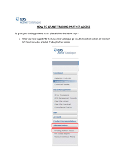


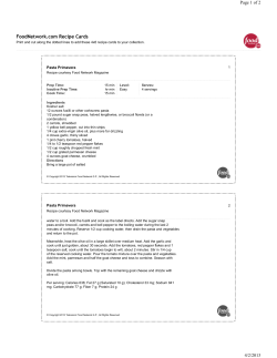


© Copyright 2026