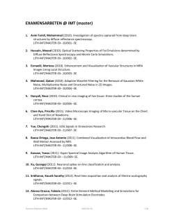
Biclustering Using Message Passing
Luke O’Connor
Bioinformatics and Integrative Genomics
Harvard University
Cambridge, MA 02138
[email protected]
Soheil Feizi
Electrical Engineering and Computer Science
Massachusetts Institute of Technology
Cambridge, MA 02139
[email protected]
Abstract
Biclustering is the analog of clustering on a bipartite graph. Existent methods infer
biclusters through local search strategies that find one cluster at a time; a common
technique is to update the row memberships based on the current column memberships, and vice versa. We propose a biclustering algorithm that maximizes a global
objective function using message passing. Our objective function closely approximates a general likelihood function, separating a cluster size penalty term into
row- and column-count penalties. Because we use a global optimization framework, our approach excels at resolving the overlaps between biclusters, which are
important features of biclusters in practice. Moreover, Expectation-Maximization
can be used to learn the model parameters if they are unknown. In simulations, we
find that our method outperforms two of the best existing biclustering algorithms,
ISA and LAS, when the planted clusters overlap. Applied to three gene expression datasets, our method finds coregulated gene clusters that have high quality in
terms of cluster size and density.
1
Introduction
The term biclustering has been used to describe several distinct problems variants. In this paper, In
this paper, we consider the problem of biclustering as a bipartite analogue of clustering: Given an
N × M matrix, a bicluster is a subset of rows that are heavily connected to a subset of columns. In
this framework, biclustering methods are data mining techniques allowing simultaneous clustering
of the rows and columns of a matrix. We suppose there are two possible distributions for edge
weights in the bipartite graph: a within-cluster distribution and a background distribution. Unlike in
the traditional clustering problem, in our setup, biclusters may overlap, and a node may not belong
to any cluster. We emphasize the distinction between biclustering and the bipartite analog of graph
partitioning, which might be called bipartitioning.
Biclustering has several noteworthy applications. It has been used to find modules of coregulated
genes using microarray gene expression data [1] and to predict tumor phenotypes from their genotypes [2]. It has been used for document classification, clustering both documents and related words
simultaneously [3]. In all of these applications, biclusters are expected to overlap with each other,
and these overlaps themselves are often of interest (e.g., if one wishes to explore the relationships
between document topics).
The biclustering problem is NP-hard (see Proposition 1). However, owing to its practical importance, several heuristic methods using local search strategies have been developed. A popular approach is to search for one bicluster at a time by iteratively assigning rows to a bicluster based on
the columns, and vice versa. Two algorithms based on this approach are ISA [4] and LAS [5]. Another approach is an exhaustive search for complete bicliques used by Bimax [6]. This approach
fragments large noisy clusters into small complete ones. SAMBA [7] uses a heuristic combinatorial
search for locally optimal biclusters, motivated by an exhaustive search algorithm that is exponential
1
in the maximum degree of the nodes. For more details about existent biclustering algorithms, and
performance comparisons, see references [6] and [8]. Existent biclustering methods have two major
shortcomings: first, they apply a local optimality criterion to each bicluster individually. Because a
collection of locally optimal biclusters might not be globally optimal, these local methods struggle
to resolve overlapping clusters, which arise frequently in many applications. Second, the lack of
a well-defined global objective function precludes an analytical characterization of their expected
results.
Global optimization methods have been developed for problems closely related to biclustering, including clustering. Unlike most biclustering problem formulations, these are mostly partitioning
problems: each node is assigned to one cluster or category. Major recent progress has been made in
the development of spectral clustering methods (see references [9] and [10]) and message-passing
algorithms (see [11], [12] and [13]). In particular, Affinity Propagation [12] maximizes the sum of
similarities to one central exemplar instead of overall cluster density. Reference [14] uses variational
expectation-maximization to fit the latent block model, which is a binary model in which each row
or column is assigned to a row or column cluster, and the probability of an edge is dictated by the
respective cluster memberships. Row and column clusters that are not paired to form biclusters.
In this paper, we propose a message-passing algorithm that searches for a globally optimal collection of possibly overlapping biclusters. Our method maximizes a likelihood function using an
approximation that separates a cluster-size penalty term into a row-count penalty and a columncount penalty. This decoupling enables the messages of the max-sum algorithm to be computed
efficiently, effectively breaking an intractable optimization into a pair of tractable ones that can be
solved in nearly linear time. When the underlying model parameters are unknown, they can be
learned using an expectation-maximization approach.
Our approach has several advantages over existing biclustering algorithms: the objective function
of our biclustering method has the flexibility to handle diverse statistical models; the max-sum algorithm is a more robust optimization strategy than commonly used iterative approaches; and in
particular, our global optimization technique excels at resolving overlapping biclusters. In simulations, our method outperforms two of the best existing biclustering algorithms, ISA and LAS, when
the planted clusters overlap. Applied to three gene expression datasets, our method found biclusters
of high quality in terms of cluster size and density.
2
2.1
Methods
Problem statement
Let G = (V, W, E) be a weighted bipartite graph, with vertices V = (1, ..., N ) and W = (1, ..., M ),
connected by edges with non-negative weights: E : V × W → [0, ∞). Let V1 , ..., VK ⊂ V and
W1 , ..., WK ⊂ W . Let (Vk , Wk ) = {(i, j) : i ∈ Vk , j ∈ Wk } be a bicluster: Graph edge weights
eij are drawn independently from either a within-cluster distribution or a background distribution
depending on whether, for some k, i ∈ Vk and j ∈ Wk . In this paper, we assume that the withincluster and background distributions are homogenous. However, our formulation can be extended
to a general case in which the distributions are row- or column-dependent.
P
Let ckij be the indicator for i ∈ Vk and j ∈ Wk . Let cij , min(1, k ckij ) and let c , (ckij ).
Definition 1 (Biclustering Problem). Let G = (V, W, E) be a bipartite graph with biclusters
(V1 , W1 ), ..., (VK , WK ), within-cluster distribution f1 and background distribution f0 . The problem
is to find the maximum likelihood cluster assignments (up to reordering):
X
f1 (eij )
ˆ = arg max
c
cij log
,
(1)
c
f0 (eij )
(i,j)
ckij = ckrs = 1 ⇒ ckis = ckrj = 1,
∀i, r ∈ V, ∀j, s ∈ W.
Figure 1 demonstrates the problem qualitatively for an unweighted bipartite graph. In general, the
combinatorial nature of a biclustering problem makes it computationally challenging.
Proposition 1. The clique problem can be reduced to the maximum likelihood problem of Definition
(1). Thus, the biclustering problem is NP-hard.
2
(a)
Biclustering
Biclustering
row variables
row variables
(b)
column variables
column variables
Figure 1: Biclustering is the analogue of clustering on a bipartite graph. (a) Biclustering allows
nodes to be reordered in a manner that reveals modular structures in the bipartite graph. (b) The
rows and columns of an adjacency matrix are similarly biclustered and reordered.
Proof. Proof is provided in Supplementary Note 1.
2.2
BCMP objective function
In this section, we introduce the global objective function considered in the proposed biclustering
algorithm called Biclustering using Message Passing (BCMP). This objective function approximates
f (e )
the likelihood function of Definition 1. Let lij = log f10 (eij
be the log-likelihood ratio score of
ij )
P
tuple (i, j). Thus, the likelihood function of Definition 1 can be written as
cij lij . If there were
no consistency constraints in the Optimization (1), an optimal maximum likelihood biclustering
solution would be to set cij = 1 for all tuples with positive lij . Our key idea is to enforce the
consistency constraints by introducing a cluster-size penalty function and shifting the log-likelihood
ratios lij to recoup this penalty. Let Nk and Mk be the number of rows and columns, respectively,
assigned to cluster k. We have,
X
(a)
cij lij ≈
(i,j)
X
cij max(0, lij + δ) − δ
(i,j)
(b)
=
X
≈
X
(i,j)
cij
(i,j)
cij max(0, lij + δ) + δ
(i,j)
(c)
X
X
max(0, −1 +
X
ckij ) − δ
k
(i,j)
cij max(0, lij + δ) + δ
X
max(0, −1 +
X
k
(i,j)
X
Nk Mk
k
ckij ) −
δX
rk Nk2 + rk−1 Mk2 .
2
k
(2)
The approximation (a) holds when δ is large enough that thresholding lij at −δ has little effect on
the resulting objective function. In equation (b), we have expressed the second term of (a) in terms
of a cluster size penalty −δNk Mk , and we have added back a term corresponding to the overlap
between clusters. Because a cluster-size penalty function of the form Nk Mk leads to an intractable
optimization in the max-sum framework, we approximate it using a decoupling approximation (c)
where rk is a cluster shape parameter:
2Nk Mk ≈ rk Nk2 + rk−1 Mk2 ,
(3)
when rk ≈ Mk /Nk . The cluster-shape parameter can be iteratively tuned to fit the estimated biclusters.
Following equation (2), the BCMP objective function can be separated into three terms as follows:
3
F (c) =
X
τij +
i,j
X
ηk +
X
k
µk ,
(4)
k
P k
P k

τij = `ij min(1, k cij ) + δ max(0, k cij − 1)
η = − 2δ rk Nk2
 k
µk = − 2δ rk−1 Mk2
∀(i, j) ∈ V × W,
∀1 ≤ k ≤ K,
∀1 ≤ k ≤ K
(5)
Here τij , the tuple function, encourages heavier edges of the bipartite graph to be clustered. Its
second term compensates for the fact that when biclusters overlap, the cluster-size penalty functions
double-count the overlapping regions. `ij , max(0, lij − δ) is the shifted log-likelihood ratio for
observed edge weight eij . ηk and µk penalize the number of rows and columns of cluster k, Nk
and Mk , respectively. Note that by introducing a penalty for each nonempty cluster, the number of
clusters can be learned, and finding weak, spurious clusters can be avoided (see Supplementary Note
3.3).
Now, we analyze BCMP over the following model for a binary or unweighted bipartite graph:
Definition 2. The binary biclustering model is a generative model for N × M bipartite graph
(V, W, E) with K biclusters distributed by uniform sampling with replacement, allowing for overlapping clusters. Within a bicluster, edges are drawn independently with probability p, and outside
of a bicluster, they are drawn independently with probability q < p.
In the following, we assume that p, q, and K are given. We discuss the case that the model parameters are unknown in Section 2.4. The following proposition shows that optimizing the BCMP
objective function solves the problem of Definition 1 in the case of the binary model:
Proposition 2. Let (eij ) be a matrix generated by the binary model described in Definition 2.
Suppose p, q and K are given. Suppose the maximum likelihood assignment of edges to biclusters,
arg max(P (data|c)), is unique up to reordering. Let rk = Mk0 /Nk0 be the cluster shape ratio for
the k-th maximum likelihood cluster. Then, by using these values of rk , setting `ij = eij , for all
(i, j), with cluster size penalty
log( 1−p
δ
1−q )
=−
,
p(1−q)
2
2 log(
)
(6)
arg max(P (data|c)) = arg max(F (c)).
(7)
q(1−p)
we have,
c
c
Proof. The proof follows the derivation of equation (2). It is presented in Supplementary Note
2.
Remark 1. In the special case when q = 1 − p ∈ (0, 1/2), according to equation (6), we have
δ
2 = 1/4. This is suggested as a reasonable initial value to choose when the true values of p and q
are unknown; see Section 2.4 for a discussion of learning the model parameters.
The assumption that rk = Nk0 /Mk0 may seem rather strong. However, it is essential as it justifies the
decoupling equation (3) that enables a linear-time algorithm. In practice, if the initial choice of rk
is close enough to the actual ratio that a cluster is detected corresponding to the real cluster, rk can
be tuned to find the true value by iteratively updating it to fit the estimated bicluster. This iterative
strategy works well in our simulations. For more details about automatically tuning the parameter
rk , see Supplementary Note 3.1.
In a more general statistical setting, log-likelihood ratios lij may be unbounded below, and the first
step (a) of derivation (2) is an approximation; setting δ arbitrarily large will eventually lead to
instability in the message updates.
4
2.3
Biclustering Using Message Passing
In this section, we use the max-sum algorithm to optimize the objective function of equation (4).
For a review of the max-sum message update rules, see Supplementary Note 4. There are N M
function nodes for the functions τij , K function nodes for the functions ηk , and K function nodes
for the functions µk . There are N M K binary variables, each attached to three function nodes: ckij
is attached to τij , ηk , and µk (see Supplementary Figure 1). The incoming messages from these
function nodes are named tkij , nkij , and mkij , respectively. In the following, we describe messages for
ckij = c112 ; other messages can be computed similarly.
First, we compute t112 :
(a)
t112 (x) =
max [τ12 (x, c212 , . . . , cK
12 ) +
c212 ,...,cK
12
(b)
=
max [`12 min(1,
c212 ,...,cK
12
X
mk12 (ck12 ) + nk12 (ck12 )]
(8)
k6=1
X
ck12 ) + δ max(0,
k
X
k
ck12 − 1) +
X
ck12 (mk12 + nk12 )] + d1
k6=1
where d1 = k6=1 mk12 (0)+nk12 (0) is a constant. Equality (a) comes from the definition of messages
according to equation (6) in the Supplement. Equality (b) uses the definition of τ12 of equation (5)
and the definition of the scalar message of equation (8) in the Supplement. We can further simplify
t12 as follows:

P
(c)
1
k
k


t12 (1) − d1 = `12 + k6=1 max(0, δ + m12 + n12 ),
P
(d)
t112 (0) − d1 = `12 − δ + k6=1 max(0, δ + mk12 + nk12 ), if ∃k, nk12 + mk12 + δ > 0, (9)


1
(e)
t12 (0) − d1 = max(0, `12 + maxk6=1 (mk12 + nk12 )),
otherwise .
P
P
P
If c112 = 1, we have min(1, k ck12 ) = 1, and max(0, k ck12 − 1) = k6=1 ck12 . These lead to
equality (c). A similar argument can be made if c112 = 0 but there exists a k such that nk12 +mk12 +δ >
0. This leads to equality (d). If c112 = 0 and there is no k such that nk12 + mk12 + δ > 0, we compare
the increase obtained by letting ck12 = 1 (i.e., `12 ) with the penalty (i.e., mk12 + nk12 ), for the best k.
This leads to equality (e).
Remark 2. Computation of t1ij , ..., tkij using equality (d) costs O(K), and not O(K 2 ), as the summation need only be computed once.
P
Messages m112 and n112 are computed as follows:
(
P
m112 (x) = maxc1 |c112 =x [µ1 (c1 ) + (i,j)6=(1,2) t1ij (c1ij ) + n1ij (c1ij )],
P
n112 (x) = maxc1 |c112 =x [η1 (c1 ) + (i,j)6=(1,2) t1ij (c1ij ) + m1ij (c1ij )],
(10)
where c1 = {c1ij : i ∈ V, j ∈ W }. To compute n112 in constant time, we perform a preliminary
optimization, ignoring the effect of edge (1, 2):
δ 2 X 1 1
N +
tij (cij ) + m1ij (c1ij ).
(11)
arg max
−
2 1
c1
(i,j)
PM
Let si = j=1 max(0, m1ij + t1ij ) be the sum of positive incoming messages of row i. The function
η1 penalizes the number of rows containing some nonzero c1ij : if any message along that row is
included, there is no additional penalty for including every positive message along that row. Thus,
optimization (11) is computed by deciding which rows to include. This can be done efficiently
through sorting: we sort row sums s(1) , ..., s(N ) at a cost of O(N log N ). Then we proceed from
largest to smallest, including row (N + 1 − i) if the marginal penalty 2δ (i2 − (i − 1)2 ) = 2δ (2i − 1)
is less than s(N +1−i) . After solving optimization (11), the messages n112 , ..., n1N 2 can be computed
in linear time, as we explain in Supplementary Note 5.
Remark 3. Computation of nkij through sorting costs O(N log N ).
Proposition 3 (Computational Complexity of BCMP). The computational complexity of BCMP
over a bipartite graph with N rows, M columns, and K clusters is O(K(N + log M )(M + log N )).
5
Proof. For each iteration, there are N M messages tij to be computed at cost O(K) each. Before
computing (nkij ), there are K sorting steps at a cost of O(M log M ), after which each message may
be computed in constant time. Likewise, there are K sorting steps at a cost of O(N log N ) each
before computing (mkij ).
We provide an empirical runtime example of the algorithm in Supplementary Figure 3.
2.4
Parameter learning using Expectation-Maximization
In the BCMP objective function described in Section 2.2, the parameters of the generative model
were used to compute the log-likelihood ratios (lij ). In practice, however, these parameters may
be unknown. Expectation-Maximization (EM) can be used to estimate these parameters. The use
of EM in this setting is slightly unorthodox, as we estimate the hidden labels (cluster assignments)
in the M step instead of the E step. However, the distinction between parameters and labels is not
intrinsic in the definition of EM [15] and the true ML solution is still guaranteed to be a fixed point
of the iterative process. Note that it is possible that the EM iterative procedure leads to a locally
optimal solution and therefore it is recommended to use several random re-initializations for the
method.
The EM algorithm has three steps:
• Initialization: We choose initial values for the underlying model parameters θ and compute
the log-likelihood ratios (lij ) based on these values, denoting by F0 the initial objective
function.
• M step: We run BCMP to maximize the objective Fi (c). We denote the estimated cluster
assignments by by cˆi .
• E step: We compute the expected-log-likelihood function as follows:
Fi+1 (c) = Eθ [log P ((eij )|θ)|c = cˆi ] =
X
Eθ [log P (eij |θ)|c = cˆi ].
(12)
(i,j)
Conveniently, the expected-likelihood function takes the same form as the original likelihood function, with an input matrix of expected log-likelihood ratios. These can be computed efficiently if
conjugate priors are available for the parameters. Therefore, BCMP can be used to maximize Fi+1 .
The algorithm terminates upon failure to improve the estimated likelihood Fi (cˆi ).
For a discussion of the application of EM to the binary and Gaussian models, see Supplementary
Note 6. In the case of the binary model, we use uniform Beta distributions as conjugate priors
for p and q, and in the case of the Gaussian model, we use inverse-gamma-normal distributions as
the priors for the variances and means. Even when convenient priors are not available, EM is still
tractable as long as one can sample from the posterior distributions.
3
Evaluation results
We compared the performance of our biclustering algorithm with two methods, ISA and LAS, in
simulations and in real gene expression datasets (Supplementary Note 8). ISA was chosen because
it performed well in comparison studies [6] [8], and LAS was chosen because it outperformed ISA
in preliminary simulations. Both ISA and LAS search for biclusters using iterative refinement. ISA
assigns rows iteratively to clusters fractionally in proportion to the sum of their entries over columns.
It repeats the same for column-cluster assignments, and this process is iterated until convergence.
LAS uses a similar greedy iterative search without fractional memberships, and it masks alreadydetected clusters by mean subtraction.
In our simulations, we generate simulated bipartite graphs of size 100x100. We planted (possibly
overlapping) biclusters as full blocks with two noise models:
• Bernoulli noise: we drew edges according to the binary model of Definition 2 with varying
noise level q = 1 − p.
6
Bernoulli noise
1400
average number of
misclassified tuples
row variables
1000
800
(a2)
total number of clustered
tuples is 850
600
400
0.05
0.1
0.15
0.2
noise level
0.25
0.3
BCMP
LAS
ISA
600
400
200
1000
0.2
0.4
0.6
0.8
1
noise level
(b2)
BCMP
LAS
ISA
1200
0
0.35
1800
1400
average number of
misclassified tuples
total number of clustered tuples is 850
800
0
0
1600
row variables
1000
200
0
column variables
average number of
misclassified tuples
BCMP
LAS
ISA
1200
overlapping biclusters
(fixed overlap)
Gaussian noise
(b1)
average number of
misclassified tuples
non-overlapping biclusters
(a1)
total number of clustered
tuples is 900
800
600
400
1000
total number of clustered tuples is 900
800
BCMP
LAS
ISA
600
400
200
200
0
column variables
overlapping biclusters
(variable overlap)
0
0.05
0.1
0.15
0.2
0.25
0.3
0
0.35
noise level
(a3)
(b3)
600
0.4
0.6
0.8
1
800
700
average number of
misclassified tuples
average number of
misclassified tuples
0.2
noise level
500
row variables
0
BCMP
LAS
400
300
200
100
600
BCMP
LAS
500
400
300
200
100
column variables
0
0
0.1
0.2
0.3
overlap
0.4
0.5
0.6
0
0
0.1
0.2
0.3
0.4
0.5
overlap
Figure 2: Performance comparison of the proposed method (BCMP) with ISA and LAS, for
Bernoulli and Gaussian models, and for overlapping and non-overlapping biclusters. On the y axis
is the total number of misclassified row-column pairs. Either the noise level or the amount of overlap
is on the x axis.
• Gaussian noise: we drew edge weights within and outside of biclusters from normal distributions N (1, σ 2 ) and N (0, σ 2 ), respectively, for different values of σ.
For each of these cases, we ran simulations on three setups (see Figure 2):
• Non-overlapping clusters: three non-overlapping biclusters were planted in a 100 × 100
matrix with sizes 20 × 20, 15 × 20, and 15 × 10. We varied the noise level.
• Overlapping clusters with fixed overlap: Three overlapping biclusters with fixed overlaps
were planted in a 100 × 100 matrix with sizes 20 × 20, 20 × 10, and 10 × 30. We varied
the noise level.
• Overlapping clusters with variable overlap: we planted two 30 × 30 biclusters in a 100 ×
100 matrix with variable amount of overlap between them, where the amount of overlap
is defined as the fraction of rows and columns shared between the two clusters. We used
Bernoulli noise level q = 1 − p = 0.15, and Gaussian noise level σ = 0.7.
The methods used have some parameters to set. Pseudocode for BCMP is presented in Supplementary Note 10. Here are the parameters that we used to run each method:
• BCMP method with underlying parameters given: We computed the input matrix of shifted
log-likelihood ratios following the discussion in Section 2.2. The number of biclusters
K was given. We initialized the cluster-shape parameters rk at 1 and updated them as
discussed in Supplementary Note 3.1. In the case of Bernoulli noise, following Proposition
2 and Remark 1, we set `ij = eij and 2δ = 1/4. In the case of Gaussian noise, we chose a
threshold δ to maximize the unthresholded likelihood (see Supplementary Note 3.2).
• BCMP - EM method: Instead of taking the underlying model parameters as given, we
estimated them using the procedure described in Section 2.4 and Supplementary Note 6.
7
We used identical, uninformative priors on the parameters of the within-cluster and null
distributions.
• ISA method: We used the same threshold ranges for both rows and columns, attempting
to find best-performing threshold values for each noise level. These values were mostly
around 1.5 for both noise types and for all three dataset types. We found positive biclusters,
and used 20 reinitializations. Out of these 20 runs, we selected the best-performing run.
• LAS method: There were no parameters to set. Since K was given, we selected the first K
biclusters discovered by LAS, which marginally increased its performance.
Evaluation results of both noise models and non-overlapping and overlapping biclusters are shown
in Figure 2. In the non-overlapping case, BCMP and LAS performed similarly well, better than
ISA. Both of these methods made few or no errors up until noise levels q = 0.2 and σ = .6 in
Bernoulli and Gaussian cases, respectively. When the parameters had to be estimated using EM,
BCMP performed worse for higher levels of Gaussian noise but well otherwise. ISA outperformed
BCMP and LAS at very high levels of Bernoulli noise; at such a high noise level, however, the
results of all three algorithms are comparable to a random guess.
In the presence of overlap between biclusters, BCMP outperformed both ISA and LAS except at very
high noise levels. Whereas LAS and ISA struggled to resolve these clusters even in the absence of
noise, BCMP made few or no errors up until noise levels q = 0.2 and σ = .6 in Bernoulli and Gaussian cases, respectively. Notably, the overlapping clusters were more asymmetrical, demonstrating
the robustness of the strategy of iteratively tuning rk in our method. In simulations with variable
overlaps between biclusters, for both noise models, BCMP outperformed LAS significantly, while
the results for the ISA method were very poor (data not shown). These results demonstrate that
BCMP excels at inferring overlapping biclusters.
4
Discussion and future directions
In this paper, we have proposed a new biclustering technique called Biclustering Using Message
Passing that, unlike existent methods, infers a globally optimal collection of biclusters rather than a
collection of locally optimal ones. This distinction is especially relevant in the presence of overlapping clusters, which are common in most applications. Such overlaps can be of importance if one is
interested in the relationships among biclusters. We showed through simulations that our proposed
method outperforms two popular existent methods, ISA and LAS, in both Bernoulli and Gaussian
noise models, when the planted biclusters were overlapping. We also found that BCMP performed
well when applied to gene expression datasets.
Biclustering is a problem that arises naturally in many applications. Often, a natural statistical model
for the data is available; for example, a Poisson model can be used for document classification (see
Supplementary Note 9). Even when no such statistical model will be available, BCMP can be used
to maximize a heuristic objective function such as the modularity function [17]. This heuristic is
preferable to clustering the original adjacency matrix when the degrees of the nodes vary widely;
see Supplementary Note 7.
The same optimization strategy used in this paper for biclustering can also be applied to perform
clustering, generalizing the graph-partitioning problem by allowing nodes to be in zero or several
clusters. We believe that the flexibility of our framework to fit various statistical and heuristic models
will allow BCMP to be used in diverse clustering and biclustering applications.
Acknowledgments
We would like to thank Professor Manolis Kellis and Professor Muriel Médard for their advice
and support. We would like to thank the Harvard Division of Medical Sciences for supporting this
project.
8
References
[1] Cheng, Yizong, and George M. Church. "Biclustering of expression data." Ismb. Vol. 8. 2000.
[2] Dao, Phuong, et al. "Inferring cancer subnetwork markers using density-constrained biclustering." Bioinformatics 26.18 (2010): i625-i631.
[3] Bisson, Gilles, and Fawad Hussain. "Chi-sim: A new similarity measure for the co-clustering
task." Machine Learning and Applications, 2008. ICMLA’08. Seventh International Conference
on. IEEE, 2008.
[4] Bergmann, Sven, Jan Ihmels, and Naama Barkai. "Iterative signature algorithm for the analysis
of large-scale gene expression data." Physical review E 67.3 (2003): 031902.
[5] Shabalin, Andrey A., et al. "Finding large average submatrices in high dimensional data." The
Annals of Applied Statistics (2009): 985-1012.
[6] Prelic, Amela, et al. "A systematic comparison and evaluation of biclustering methods for gene
expression data." Bioinformatics 22.9 (2006): 1122-1129.
[7] Tanay, Amos, Roded Sharan, and Ron Shamir. "Discovering statistically significant biclusters
in gene expression data." Bioinformatics 18.suppl 1 (2002): S136-S144.
[8] Li, Li, et al. "A comparison and evaluation of five biclustering algorithms by quantifying goodness of biclusters for gene expression data." BioData mining 5.1 (2012): 1-10.
[9] Nadakuditi, Raj Rao, and Mark EJ Newman. "Graph spectra and the detectability of community
structure in networks." Physical review letters 108.18 (2012): 188701.
[10] Krzakala, Florent, et al. "Spectral redemption in clustering sparse networks." Proceedings of
the National Academy of Sciences 110.52 (2013): 20935-20940.
[11] Decelle, Aurelien, et al. "Asymptotic analysis of the stochastic block model for modular networks and its algorithmic applications." Physical Review E 84.6 (2011): 066106.
[12] Frey, Brendan J., and Delbert Dueck. "Clustering by passing messages between data points."
Science 315.5814 (2007): 972-976.
[13] Dueck, Delbert, et al. "Constructing treatment portfolios using affinity propagation." Research
in Computational Molecular Biology. Springer Berlin Heidelberg, 2008.
[14] Govaert, G. and Nadif, M. "Block clustering with bernoulli mixture models: Comparison of
different approaches." Computational Statistics and Data Analysis, 52 (2008): 3233-3245.
[15] Dempster, Arthur P., Nan M. Laird, and Donald B. Rubin. "Maximum likelihood from incomplete data via the EM algorithm." Journal of the Royal Statistical Society. Series B (Methodological) (1977): 1-38.
[16] Marbach, Daniel, et al. "Wisdom of crowds for robust gene network inference." Nature methods 9.8 (2012): 796-804.
[17] Newman, Mark EJ. "Modularity and community structure in networks." Proceedings of the
National Academy of Sciences 103.23 (2006): 8577-8582.
[18] Yedidia, Jonathan S., William T. Freeman, and Yair Weiss. "Constructing free-energy approximations and generalized belief propagation algorithms." Information Theory, IEEE Transactions
on 51.7 (2005): 2282-2312.
[19] Caldas, José, and Samuel Kaski. "Bayesian biclustering with the plaid model." Machine Learning for Signal Processing, 2008. MLSP 2008. IEEE Workshop on. IEEE, 2008.
9