Recurrent Models of Visual Attention
Volodymyr Mnih
Nicolas Heess Alex Graves
Google DeepMind
Koray Kavukcuoglu
{vmnih,heess,gravesa,korayk} @ google.com
Abstract
Applying convolutional neural networks to large images is computationally expensive because the amount of computation scales linearly with the number of
image pixels. We present a novel recurrent neural network model that is capable of extracting information from an image or video by adaptively selecting
a sequence of regions or locations and only processing the selected regions at
high resolution. Like convolutional neural networks, the proposed model has a
degree of translation invariance built-in, but the amount of computation it performs can be controlled independently of the input image size. While the model
is non-differentiable, it can be trained using reinforcement learning methods to
learn task-specific policies. We evaluate our model on several image classification
tasks, where it significantly outperforms a convolutional neural network baseline
on cluttered images, and on a dynamic visual control problem, where it learns to
track a simple object without an explicit training signal for doing so.
1
Introduction
Neural network-based architectures have recently had great success in significantly advancing the
state of the art on challenging image classification and object detection datasets [8, 12, 19]. Their
excellent recognition accuracy, however, comes at a high computational cost both at training and
testing time. The large convolutional neural networks typically used currently take days to train on
multiple GPUs even though the input images are downsampled to reduce computation [12]. In the
case of object detection processing a single image at test time currently takes seconds when running
on a single GPU [8, 19] as these approaches effectively follow the classical sliding window paradigm
from the computer vision literature where a classifier, trained to detect an object in a tightly cropped
bounding box, is applied independently to thousands of candidate windows from the test image at
different positions and scales. Although some computations can be shared, the main computational
expense for these models comes from convolving filter maps with the entire input image, therefore
their computational complexity is at least linear in the number of pixels.
One important property of human perception is that one does not tend to process a whole scene
in its entirety at once. Instead humans focus attention selectively on parts of the visual space to
acquire information when and where it is needed, and combine information from different fixations
over time to build up an internal representation of the scene [18], guiding future eye movements
and decision making. Focusing the computational resources on parts of a scene saves “bandwidth”
as fewer “pixels” need to be processed. But it also substantially reduces the task complexity as
the object of interest can be placed in the center of the fixation and irrelevant features of the visual
environment (“clutter”) outside the fixated region are naturally ignored.
In line with its fundamental role, the guidance of human eye movements has been extensively studied
in neuroscience and cognitive science literature. While low-level scene properties and bottom up
processes (e.g. in the form of saliency; [11]) play an important role, the locations on which humans
fixate have also been shown to be strongly task specific (see [9] for a review and also e.g. [15, 22]). In
this paper we take inspiration from these results and develop a novel framework for attention-based
task-driven visual processing with neural networks. Our model considers attention-based processing
1
of a visual scene as a control problem and is general enough to be applied to static images, videos,
or as a perceptual module of an agent that interacts with a dynamic visual environment (e.g. robots,
computer game playing agents).
The model is a recurrent neural network (RNN) which processes inputs sequentially, attending to
different locations within the images (or video frames) one at a time, and incrementally combines
information from these fixations to build up a dynamic internal representation of the scene or environment. Instead of processing an entire image or even bounding box at once, at each step, the model
selects the next location to attend to based on past information and the demands of the task. Both
the number of parameters in our model and the amount of computation it performs can be controlled
independently of the size of the input image, which is in contrast to convolutional networks whose
computational demands scale linearly with the number of image pixels. We describe an end-to-end
optimization procedure that allows the model to be trained directly with respect to a given task and
to maximize a performance measure which may depend on the entire sequence of decisions made by
the model. This procedure uses backpropagation to train the neural-network components and policy
gradient to address the non-differentiabilities due to the control problem.
We show that our model can learn effective task-specific strategies for where to look on several
image classification tasks as well as a dynamic visual control problem. Our results also suggest that
an attention-based model may be better than a convolutional neural network at both dealing with
clutter and scaling up to large input images.
2
Previous Work
Computational limitations have received much attention in the computer vision literature. For instance, for object detection, much work has been dedicated to reducing the cost of the widespread
sliding window paradigm, focusing primarily on reducing the number of windows for which the
full classifier is evaluated, e.g. via classifier cascades (e.g. [7, 24]), removing image regions from
consideration via a branch and bound approach on the classifier output (e.g. [13]), or by proposing
candidate windows that are likely to contain objects (e.g. [1, 23]). Even though substantial speedups
may be obtained with such approaches, and some of these can be combined with or used as an add-on
to CNN classifiers [8], they remain firmly rooted in the window classifier design for object detection
and only exploit past information to inform future processing of the image in a very limited way.
A second class of approaches that has a long history in computer vision and is strongly motivated
by human perception are saliency detectors (e.g. [11]). These approaches prioritize the processing
of potentially interesting (“salient”) image regions which are typically identified based on some
measure of local low-level feature contrast. Saliency detectors indeed capture some of the properties
of human eye movements, but they typically do not to integrate information across fixations, their
saliency computations are mostly hardwired, and they are based on low-level image properties only,
usually ignoring other factors such as semantic content of a scene and task demands (but see [22]).
Some works in the computer vision literature and elsewhere e.g. [2, 4, 6, 14, 16, 17, 20] have embraced vision as a sequential decision task as we do here. There, as in our work, information about
the image is gathered sequentially and the decision where to attend next is based on previous fixations of the image. [4] employs the learned Bayesian observer model from [5] to the task of object
detection. The learning framework of [5] is related to ours as they also employ a policy gradient
formulation (cf. section 3) but their overall setup is considerably more restrictive than ours and only
some parts of the system are learned.
Our work is perhaps the most similar to the other attempts to implement attentional processing in a
deep learning framework [6, 14, 17]. Our formulation which employs an RNN to integrate visual
information over time and to decide how to act is, however, more general, and our learning procedure
allows for end-to-end optimization of the sequential decision process instead of relying on greedy
action selection. We further demonstrate how the same general architecture can be used for efficient
object recognition in still images as well as to interact with a dynamic visual environment in a
task-driven way.
3
The Recurrent Attention Model (RAM)
In this paper we consider the attention problem as the sequential decision process of a goal-directed
agent interacting with a visual environment. At each point in time, the agent observes the environment only via a bandwidth-limited sensor, i.e. it never senses the environment in full. It may extract
2
A)
C)
lt-1
ρ(xt , lt-1)
xt
fg(θg)
Glimpse Sensor
B)
ρ(xt , lt-1)
xt
θg1
Glimpse Network :
fg(θg)
gt
ht-1
θg0
Glimpse
Sensor
lt-1
lt
lt-1
θg2
gt
fg( θg )
gt+1
ht
ht+1
fh(θh)
fh(θh)
fa(θa)
fl(θl)
fa(θa)
fl(θl)
at
lt
at+1
lt+1
Figure 1: A) Glimpse Sensor: Given the coordinates of the glimpse and an input image, the sensor extracts a retina-like representation ρ(xt , lt−1 ) centered at lt−1 that contains multiple resolution
patches. B) Glimpse Network: Given the location (lt−1 ) and input image (xt ), uses the glimpse
sensor to extract retina representation ρ(xt , lt−1 ). The retina representation and glimpse location is
then mapped into a hidden space using independent linear layers parameterized by θg0 and θg1 respectively using rectified units followed by another linear layer θg2 to combine the information from both
components. The glimpse network fg (.; {θg0 , θg1 , θg2 }) defines a trainable bandwidth limited sensor
for the attention network producing the glimpse representation gt . C) Model Architecture: Overall,
the model is an RNN. The core network of the model fh (.; θh ) takes the glimpse representation gt as
input and combining with the internal representation at previous time step ht−1 , produces the new
internal state of the model ht . The location network fl (.; θl ) and the action network fa (.; θa ) use the
internal state ht of the model to produce the next location to attend to lt and the action/classification
at respectively. This basic RNN iteration is repeated for a variable number of steps.
information only in a local region or in a narrow frequency band. The agent can, however, actively
control how to deploy its sensor resources (e.g. choose the sensor location). The agent can also
affect the true state of the environment by executing actions. Since the environment is only partially
observed the agent needs to integrate information over time in order to determine how to act and
how to deploy its sensor most effectively. At each step, the agent receives a scalar reward (which
depends on the actions the agent has executed and can be delayed), and the goal of the agent is to
maximize the total sum of such rewards.
This formulation encompasses tasks as diverse as object detection in static images and control problems like playing a computer game from the image stream visible on the screen. For a game, the
environment state would be the true state of the game engine and the agent’s sensor would operate
on the video frame shown on the screen. (Note that for most games, a single frame would not fully
specify the game state). The environment actions here would correspond to joystick controls, and
the reward would reflect points scored. For object detection in static images the state of the environment would be fixed and correspond to the true contents of the image. The environmental action
would correspond to the classification decision (which may be executed only after a fixed number
of fixations), and the reward would reflect if the decision is correct.
3.1 Model
The agent is built around a recurrent neural network as shown in Fig. 1. At each time step, it
processes the sensor data, integrates information over time, and chooses how to act and how to
deploy its sensor at next time step:
Sensor: At each step t the agent receives a (partial) observation of the environment in the form of
an image xt . The agent does not have full access to this image but rather can extract information
from xt via its bandwidth limited sensor ρ, e.g. by focusing the sensor on some region or frequency
band of interest.
In this paper we assume that the bandwidth-limited sensor extracts a retina-like representation
ρ(xt , lt−1 ) around location lt−1 from image xt . It encodes the region around l at a high-resolution
but uses a progressively lower resolution for pixels further from l, resulting in a vector of much
3
lower dimensionality than the original image x. We will refer to this low-resolution representation
as a glimpse [14]. The glimpse sensor is used inside what we call the glimpse network fg to produce
the glimpse feature vector gt = fg (xt , lt−1 ; θg ) where θg = {θg0 , θg1 , θg2 } (Fig. 1B).
Internal state: The agent maintains an interal state which summarizes information extracted from
the history of past observations; it encodes the agent’s knowledge of the environment and is instrumental to deciding how to act and where to deploy the sensor. This internal state is formed
by the hidden units ht of the recurrent neural network and updated over time by the core network:
ht = fh (ht−1 , gt ; θh ). The external input to the network is the glimpse feature vector gt .
Actions: At each step, the agent performs two actions: it decides how to deploy its sensor via the
sensor control lt , and an environment action at which might affect the state of the environment.
The nature of the environment action depends on the task. In this work, the location actions are
chosen stochastically from a distribution parameterized by the location network fl (ht ; θl ) at time t:
lt ∼ p(·|fl (ht ; θl )). The environment action at is similarly drawn from a distribution conditioned
on a second network output at ∼ p(·|fa (ht ; θa )). For classification it is formulated using a softmax
output and for dynamic environments, its exact formulation depends on the action set defined for
that particular environment (e.g. joystick movements, motor control, ...). Finally, our model can
also be augmented with an additional action that decides when it will stop taking glimpses. This
could, for example, be used to learn a cost-sensitive classifier by giving the agent a negative reward
for each glimpse it takes, forcing it to trade off making correct classifications with the cost of taking
more glimpses.
Reward: After executing an action the agent receives a new visual observation of the environment
xt+1 and a reward signal rt+1 . The goal of the agent is to maximize the sum of the reward signal1
PT
which is usually very sparse and delayed: R =
t=1 rt . In the case of object recognition, for
example, rT = 1 if the object is classified correctly after T steps and 0 otherwise.
The above setup is a special instance of what is known in the RL community as a Partially Observable Markov Decision Process (POMDP). The true state of the environment (which can be static or
dynamic) is unobserved. In this view, the agent needs to learn a (stochastic) policy π((lt , at )|s1:t ; θ)
with parameters θ that, at each step t, maps the history of past interactions with the environment
s1:t = x1 , l1 , a1 , . . . xt−1 , lt−1 , at−1 , xt to a distribution over actions for the current time step, subject to the constraint of the sensor. In our case, the policy π is defined by the RNN outlined above,
and the history st is summarized in the state of the hidden units ht . We will describe the specific
choices for the above components in Section 4.
3.2 Training
The parameters of our agent are given by the parameters of the glimpse network, the core network
(Fig. 1C), and the action network θ = {θg , θh , θa } and we learn these to maximize the total reward
the agent can expect when interacting with the environment.
More formally, the policy of the agent, possibly in combination with the dynamics of the environment (e.g. for game-playing), induces a distribution over possible interaction
s1:N and we
i
hP sequences
T
aim to maximize the reward under this distribution: J(θ) = Ep(s1:T ;θ)
r
=
E
p(s1:T ;θ) [R],
t=1 t
where p(s1:T ; θ) depends on the policy
Maximizing J exactly is non-trivial since it involves an expectation over the high-dimensional interaction sequences which may in turn involve unknown environment dynamics. Viewing the problem
as a POMDP, however, allows us to bring techniques from the RL literature to bear: As shown by
Williams [26] a sample approximation to the gradient is given by
∇θ J =
T
X
Ep(s1:T ;θ) [∇θ log π(ut |s1:t ; θ)R] ≈
t=1
M T
1 XX
∇θ log π(uit |si1:t ; θ)Ri ,
M i=1 t=1
(1)
where si ’s are interaction sequences obtained by running the current agent πθ for i = 1 . . . M
episodes.
1
Depending on the scenario it may be more appropriate to consider a sum of discounted rewards, where
P
rewards obtained in the distant future contribute less: R = Tt=1 γ t−1 rt . In this case we can have T → ∞.
4
The learning rule (1) is also known as the REINFORCE rule, and it involves running the agent with
its current policy to obtain samples of interaction sequences s1:T and then adjusting the parameters
θ of our agent such that the log-probability of chosen actions that have led to high cumulative reward
is increased, while that of actions having produced low reward is decreased.
Eq. (1) requires us to compute ∇θ log π(uit |si1:t ; θ). But this is just the gradient of the RNN that
defines our agent evaluated at time step t and can be computed by standard backpropagation [25].
Variance Reduction : Equation (1) provides us with an unbiased estimate of the gradient but it may
have high variance. It is therefore common to consider a gradient estimate of the form
M T
1 XX
∇θ log π(uit |si1:t ; θ) Rti − bt ,
M i=1 t=1
(2)
PT
where Rti = t0 =1 rti0 is the cumulative reward obtained following the execution of action uit , and
bt is a baseline that may depend on si1:t (e.g. via hit ) but not on the action uit itself. This estimate
is equal to (1) in expectation but may have lower variance. It is natural to select bt = Eπ [Rt ] [21],
and this form of baseline known as the value function in the reinforcement learning literature. The
resulting algorithm increases the log-probability of an action that was followed by a larger than
expected cumulative reward, and decreases the probability if the obtained cumulative reward was
smaller. We use this type of baseline and learn it by reducing the squared error between Rti ’s and bt .
Using a Hybrid Supervised Loss: The algorithm described above allows us to train the agent when
the “best” actions are unknown, and the learning signal is only provided via the reward. For instance,
we may not know a priori which sequence of fixations provides most information about an unknown
image, but the total reward at the end of an episode will give us an indication whether the tried
sequence was good or bad.
However, in some situations we do know the correct action to take: For instance, in an object
detection task the agent has to output the label of the object as the final action. For the training
images this label will be known and we can directly optimize the policy to output the correct label
associated with a training image at the end of an observation sequence. This can be achieved, as is
common in supervised learning, by maximizing the conditional probability of the true label given
the observations from the image, i.e. by maximizing log π(a∗T |s1:T ; θ), where a∗T corresponds to the
ground-truth label(-action) associated with the image from which observations s1:T were obtained.
We follow this approach for classification problems where we optimize the cross entropy loss to
train the action network fa and backpropagate the gradients through the core and glimpse networks.
The location network fl is always trained with REINFORCE.
4
Experiments
We evaluated our approach on several image classification tasks as well as a simple game. We first
describe the design choices that were common to all our experiments:
Retina and location encodings: The retina encoding ρ(x, l) extracts k square patches centered at
location l, with the first patch being gw × gw pixels in size, and each successive patch having twice
the width of the previous. The k patches are then all resized to gw × gw and concatenated. Glimpse
locations l were encoded as real-valued (x, y) coordinates2 with (0, 0) being the center of the image
x and (−1, −1) being the top left corner of x.
Glimpse network: The glimpse network fg (x, l) had two fully connected layers. Let Linear(x) denote a linear transformation of the vector x, i.e. Linear(x) = W x+b for some weight matrix W and
bias vector b, and let Rect(x) = max(x, 0) be the rectifier nonlinearity. The output g of the glimpse
network was defined as g = Rect(Linear(hg ) + Linear(hl )) where hg = Rect(Linear(ρ(x, l)))
and hl = Rect(Linear(l)). The dimensionality of hg and hl was 128 while the dimensionality of
g was 256 for all attention models trained in this paper.
Location network: The policy for the locations l was defined by a two-component Gaussian with a
fixed variance. The location network outputs the mean of the location policy at time t and is defined
as fl (h) = Linear(h) where h is the state of the core network/RNN.
2
We also experimented with using a discrete representation for the locations l but found that it was difficult
to learn policies over more than 25 possible discrete locations.
5
(a) 28x28 MNIST
Model
FC, 2 layers (256 hiddens each)
Convolutional, 2 layers
RAM, 2 glimpses, 8 × 8, 1 scale
RAM, 3 glimpses, 8 × 8, 1 scale
RAM, 4 glimpses, 8 × 8, 1 scale
RAM, 5 glimpses, 8 × 8, 1 scale
RAM, 6 glimpses, 8 × 8, 1 scale
RAM, 7 glimpses, 8 × 8, 1 scale
Error
1.69%
1.21%
3.79%
1.51%
1.54%
1.34%
1.12%
1.07%
(b) 60x60 Translated MNIST
Model
FC, 2 layers (64 hiddens each)
FC, 2 layers (256 hiddens each)
Convolutional, 2 layers
RAM, 4 glimpses, 12 × 12, 3 scales
RAM, 6 glimpses, 12 × 12, 3 scales
RAM, 8 glimpses, 12 × 12, 3 scales
Error
6.42%
2.63%
1.62%
1.54%
1.22%
1.2%
Table 1: Classification results on the MNIST and Translated MNIST datasets. FC denotes a fullyconnected network with two layers of rectifier units. The convolutional network had one layer of 8
10 × 10 filters with stride 5, followed by a fully connected layer with 256 units with rectifiers after
each layer. Instances of the attention model are labeled with the number of glimpses, the number of
scales in the retina, and the size of the retina.
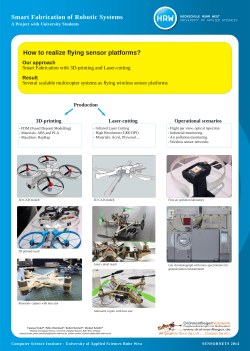
(a) Translated MNIST inputs.
(b) Cluttered Translated MNIST inputs.
Figure 2: Examples of test cases for the Translated and Cluttered Translated MNIST tasks.
Core network: For the classification experiments that follow the core fh was a network of rectifier
units defined as ht = fh (ht−1 ) = Rect(Linear(ht−1 ) + Linear(gt )). The experiment done on a
dynamic environment used a core of LSTM units [10].
4.1
Image Classification
The attention network used in the following classification experiments made a classification decision
only at the last timestep t = N . The action network fa was simply a linear softmax classifier defined
as fa (h) = exp (Linear(h)) /Z, where Z is a normalizing constant. The RNN state vector h had
dimensionality 256. All methods were trained using stochastic gradient descent with minibatches
of size 20 and momentum of 0.9. We annealed the learning rate linearly from its initial value to 0
over the course of training. Hyperparameters such as the initial learning rate and the variance of the
location policy were selected using random search [3]. The reward at the last time step was 1 if the
agent classified correctly and 0 otherwise. The rewards for all other timesteps were 0.
Centered Digits: We first tested the ability of our training method to learn successful glimpse
policies by using it to train RAM models with up to 7 glimpses on the MNIST digits dataset. The
“retina” for this experiment was simply an 8 × 8 patch, which is only big enough to capture a part of
a digit, hence the experiment also tested the ability of RAM to combine information from multiple
glimpses. We also trained standard feedforward and convolutional neural networks with two hidden
layers as a baselines. The error rates achieved by the different models on the test set are shown in
Table 1a. We see that the performance of RAM generally improves with more glimpses, and that
it eventually outperforms a the baseline models trained on the full 28 × 28 centered digits. This
demonstrates the model can successfully learn to combine information from multiple glimpses.
Non-Centered Digits: The second problem we considered was classifying non-centered digits. We
created a new task called Translated MNIST, for which data was generated by placing an MNIST
digit in a random location of a larger blank patch. Training cases were generated on the fly so the
effective training set size was 50000 (the size of the MNIST training set) multiplied by the possible
number of locations. Figure 2a contains a random sample of test cases for the 60 by 60 Translated
MNIST task. Table 1b shows the results for several different models trained on the Translated
MNIST task with 60 by 60 patches. In addition to RAM and two fully-connected networks we
also trained a network with one convolutional layer of 16 10 × 10 filters with stride 5 followed
by a rectifier nonlinearity and then a fully-connected layer of 256 rectifier units. The convolutional
network, the RAM networks, and the smaller fully connected model all had roughly the same number
of parameters. Since the convolutional network has some degree of translation invariance built in, it
6
(a) 60x60 Cluttered Translated MNIST
Model
Error
FC, 2 layers (64 hiddens each)
28.58%
FC, 2 layers (256 hiddens each)
11.96%
Convolutional, 2 layers
8.09%
RAM, 4 glimpses, 12 × 12, 3 scales 4.96%
RAM, 6 glimpses, 12 × 12, 3 scales 4.08%
RAM, 8 glimpses, 12 × 12, 3 scales 4.04%
RAM, 8 random glimpses
14.4%
(b) 100x100 Cluttered Translated MNIST
Model
Error
Convolutional, 2 layers
14.35%
RAM, 4 glimpses, 12 × 12, 4 scales 9.41%
RAM, 6 glimpses, 12 × 12, 4 scales 8.31%
RAM, 8 glimpses, 12 × 12, 4 scales 8.11%
RAM, 8 random glimpses
28.4%
Table 2: Classification on the Cluttered Translated MNIST dataset. FC denotes a fully-connected
network with two layers of rectifier units. The convolutional network had one layer of 8 10 × 10
filters with stride 5, followed by a fully connected layer with 256 units in the 60 × 60 case and
86 units in the 100 × 100 case with rectifiers after each layer. Instances of the attention model are
labeled with the number of glimpses, the size of the retina, and the number of scales in the retina.
All models except for the big fully connected network had roughly the same number of parameters.
Figure 3: Examples of the learned policy on 60 × 60 cluttered-translated MNIST task. Column 1:
The input image with glimpse path overlaid in green. Columns 2-7: The six glimpses the network
chooses. The center of each image shows the full resolution glimpse, the outer low resolution areas
are obtained by upscaling the low resolution glimpses back to full image size. The glimpse paths
clearly show that the learned policy avoids computation in empty or noisy parts of the input space
and directly explores the area around the object of interest.
attains a significantly lower error rate of 1.62% than the fully connected networks. However, RAM
with 4 glimpses gets slightly better performance than the convolutional network and outperforms
it further for 6 and 8 glimpses, reaching 1.2% error. This is possible because the attention model
can focus its retina on the digit and hence learn a translation invariant policy. This experiment also
shows that the attention model is able to successfully search for an object in a big image when the
object is not centered.
Cluttered Non-Centered Digits: One of the most challenging aspects of classifying real-world
images is the presence of a wide range clutter. Systems that operate on the entire image at full
resolution are particularly susceptible to clutter and must learn to be invariant to it. One possible
advantage of an attention mechanism is that it may make it easier to learn in the presence of clutter
by focusing on the relevant part of the image and ignoring the irrelevant part. We test this hypothesis
with several experiments on a new task we call Cluttered Translated MNIST. Data for this task was
generated by first placing an MNIST digit in a random location of a larger blank image and then
adding random 8 by 8 subpatches from other random MNIST digits to random locations of the
image. The goal is to classify the complete digit present in the image. Figure 2b shows a random
sample of test cases for the 60 by 60 Cluttered Translated MNIST task.
Table 2a shows the classification results for the models we trained on 60 by 60 Cluttered Translated
MNIST with 4 pieces of clutter. The presence of clutter makes the task much more difficult but the
performance of the attention model is affected less than the performance of the other models. RAM
with 4 glimpses reaches 4.96% error, which outperforms fully-connected models by a wide margin
and the convolutional neural network by over 3%, and RAM trained with 6 and 8 glimpses achieves
even lower error. Since RAM achieves larger relative error improvements over a convolutional
network in the presence of clutter these results suggest the attention-based models may be better at
dealing with clutter than convolutional networks because they can simply ignore it by not looking at
it. Two samples of learned policy is shown in Figure 3 and more are included in the supplementary
materials. The first column shows the original data point with the glimpse path overlaid. The
7
location of the first glimpse is marked with a filled circle and the location of the final glimpse is
marked with an empty circle. The intermediate points on the path are traced with solid straight lines.
Each consecutive image to the right shows a representation of the glimpse that the network sees. It
can be seen that the learned policy can reliably find and explore around the object of interest while
avoiding clutter at the same time. Finally, Table 2a also includes results for an 8-glimpse RAM
model that selects glimpse locations uniformly at random. RAM models that learn the glimpse
policy achieve much lower error rates even with half as many glimpses.
To further test this hypothesis we also performed experiments on 100 by 100 Cluttered Translated
MNIST with 8 pieces of clutter. The test errors achieved by the models we compared are shown
in Table 2b. The results show similar improvements of RAM over a convolutional network. It has
to be noted that the overall capacity and the amount of computation of our model does not change
from 60 × 60 images to 100 × 100, whereas the hidden layer of the convolutional network that is
connected to the linear layer grows linearly with the number of pixels in the input.
4.2 Dynamic Environments
One appealing property of the recurrent attention model is that it can be applied to videos or interactive problems with a visual input just as easily as to static image tasks. We test the ability of our
approach to learn a control policy in a dynamic visual environment while perceiving the environment
through a bandwidth-limited retina by training it to play a simple game. The game is played on a 24
by 24 screen of binary pixels and involves two objects: a single pixel that represents a ball falling
from the top of the screen while bouncing off the sides of the screen and a two-pixel paddle positioned at the bottom of the screen which the agent controls with the aim of catching the ball. When
the falling pixel reaches the bottom of the screen the agent either gets a reward of 1 if the paddle
overlaps with the ball and a reward of 0 otherwise. The game then restarts from the beginning.
We trained the recurrent attention model to play the game of “Catch” using only the final reward
as input. The network had a 6 by 6 retina at three scales as its input, which means that the agent
had to capture the ball in the 6 by 6 highest resolution region in order to know its precise position.
In addition to the two location actions, the attention model had three game actions (left, right, and
do nothing) and the action network fa used a linear softmax to model a distribution over the game
actions. We used a core network of 256 LSTM units.
We performed random search to find suitable hyper-parameters and trained each agent for 20 million frames. A video of the best agent, which catches the ball roughly 85% of the time, can
be downloaded from http://www.cs.toronto.edu/˜vmnih/docs/attention.mov.
The video shows that the recurrent attention model learned to play the game by tracking the ball
near the bottom of the screen. Since the agent was not in any way told to track the ball and was
only rewarded for catching it, this result demonstrates the ability of the model to learn effective
task-specific attention policies.
5
Discussion
This paper introduced a novel visual attention model that is formulated as a single recurrent neural
network which takes a glimpse window as its input and uses the internal state of the network to
select the next location to focus on as well as to generate control signals in a dynamic environment.
Although the model is not differentiable, the proposed unified architecture is trained end-to-end
from pixel inputs to actions using a policy gradient method. The model has several appealing properties. First, both the number of parameters and the amount of computation RAM performs can
be controlled independently of the size of the input images. Second, the model is able to ignore
clutter present in an image by centering its retina on the relevant regions. Our experiments show that
RAM significantly outperforms a convolutional architecture with a comparable number of parameters on a cluttered object classification task. Additionally, the flexibility of our approach allows for
a number of interesting extensions. For example, the network can be augmented with another action
that allows it terminate at any time point and make a final classification decision. Our preliminary
experiments show that this allows the network to learn to stop taking glimpses once it has enough information to make a confident classification. The network can also be allowed to control the scale at
which the retina samples the image allowing it to fit objects of different size in the fixed size retina.
In both cases, the extra actions can be simply added to the action network fa and trained using the
policy gradient procedure we have described. Given the encouraging results achieved by RAM, applying the model to large scale object recognition and video classification is a natural direction for
future work.
8
References
[1] Bogdan Alexe, Thomas Deselaers, and Vittorio Ferrari. What is an object? In CVPR, 2010.
[2] Bogdan Alexe, Nicolas Heess, Yee Whye Teh, and Vittorio Ferrari. Searching for objects driven by
context. In NIPS, 2012.
[3] James Bergstra and Yoshua Bengio. Random search for hyper-parameter optimization. The Journal of
Machine Learning Research, 13:281–305, 2012.
[4] Nicholas J. Butko and Javier R. Movellan. Optimal scanning for faster object detection. In CVPR, 2009.
[5] N.J. Butko and J.R. Movellan. I-pomdp: An infomax model of eye movement. In Proceedings of the 7th
IEEE International Conference on Development and Learning, ICDL ’08, pages 139 –144, 2008.
[6] Misha Denil, Loris Bazzani, Hugo Larochelle, and Nando de Freitas. Learning where to attend with deep
architectures for image tracking. Neural Computation, 24(8):2151–2184, 2012.
[7] Pedro F. Felzenszwalb, Ross B. Girshick, and David A. McAllester. Cascade object detection with deformable part models. In CVPR, 2010.
[8] Ross B. Girshick, Jeff Donahue, Trevor Darrell, and Jitendra Malik. Rich feature hierarchies for accurate
object detection and semantic segmentation. CoRR, abs/1311.2524, 2013.
[9] Mary Hayhoe and Dana Ballard. Eye movements in natural behavior. Trends in Cognitive Sciences,
9(4):188 – 194, 2005.
[10] Sepp Hochreiter and J¨urgen Schmidhuber. Long short-term memory. Neural computation, 9(8):1735–
1780, 1997.
[11] L. Itti, C. Koch, and E. Niebur. A model of saliency-based visual attention for rapid scene analysis. IEEE
Transactions on Pattern Analysis and Machine Intelligence, 20(11):1254–1259, 1998.
[12] Alex Krizhevsky, Ilya Sutskever, and Geoff Hinton. Imagenet classification with deep convolutional
neural networks. In Advances in Neural Information Processing Systems 25, pages 1106–1114, 2012.
[13] Christoph H. Lampert, Matthew B. Blaschko, and Thomas Hofmann. Beyond sliding windows: Object
localization by efficient subwindow search. In CVPR, 2008.
[14] Hugo Larochelle and Geoffrey E. Hinton. Learning to combine foveal glimpses with a third-order boltzmann machine. In NIPS, 2010.
[15] Stefan Mathe and Cristian Sminchisescu. Action from still image dataset and inverse optimal control to
learn task specific visual scanpaths. In NIPS, 2013.
[16] Lucas Paletta, Gerald Fritz, and Christin Seifert. Q-learning of sequential attention for visual object
recognition from informative local descriptors. In CVPR, 2005.
[17] M. Ranzato. On Learning Where To Look. ArXiv e-prints, 2014.
[18] Ronald A. Rensink. The dynamic representation of scenes. Visual Cognition, 7(1-3):17–42, 2000.
[19] Pierre Sermanet, David Eigen, Xiang Zhang, Micha¨el Mathieu, Rob Fergus, and Yann LeCun. Overfeat:
Integrated recognition, localization and detection using convolutional networks. CoRR, abs/1312.6229,
2013.
[20] Kenneth O. Stanley and Risto Miikkulainen. Evolving a roving eye for go. In GECCO, 2004.
[21] Richard S. Sutton, David Mcallester, Satinder Singh, and Yishay Mansour. Policy gradient methods for
reinforcement learning with function approximation. In NIPS, pages 1057–1063. MIT Press, 2000.
[22] Antonio Torralba, Aude Oliva, Monica S Castelhano, and John M Henderson. Contextual guidance of eye
movements and attention in real-world scenes: the role of global features in object search. Psychol Rev,
pages 766–786, 2006.
[23] K E A van de Sande, J.R.R. Uijlings, T Gevers, and A.W.M. Smeulders. Segmentation as Selective Search
for Object Recognition. In ICCV, 2011.
[24] Paul A. Viola and Michael J. Jones. Rapid object detection using a boosted cascade of simple features. In
CVPR, 2001.
[25] Daan Wierstra, Alexander Foerster, Jan Peters, and Juergen Schmidhuber. Solving deep memory pomdps
with recurrent policy gradients. In ICANN. 2007.
[26] R.J. Williams. Simple statistical gradient-following algorithms for connectionist reinforcement learning.
Machine Learning, 8(3):229–256, 1992.
9