ABC
docz
Explore
Log in
Create new account
Download
Report
science
weather
- IOPscience
High-Fiber Power Pudding Recipe
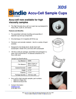
Accu-Cell Sample Cups Accu-cell now available for high viscosity samples
TEM imaging of tip-sample contacts between
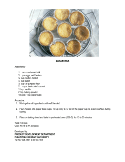
MACAROONS Ingredients: 1 can condensed milk
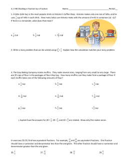
3.1 HW Dividing a Fraction by a Fraction Name:____________________________________Period:__
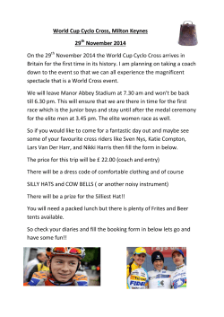
World Cup Cyclo Cross, Milton Keynes 29 November 2014 On the 29
How to make a Weather Vane and an Anemometer Background information
BLOG - Recipes & How To's
Document 418539
10905_Davis Cup Anemometer_Web
Document
User Manual - Gill Instruments
© Copyright 2026
About abcdocz
DMCA / GDPR
Report