Earth’s Future
RESEARCH ARTICLE
10.1002/2014EF000265
Key Points:
• Emissions of oil and gas industries
are constrained using satellite
observations
• Current inventories likely
underestimate fugitive methane
emissions
• Climate beneﬁt of transition to
unconventional oil and gas is
questionable
Corresponding author:
O. Schneising, oliver.schneising@iup.
physik.uni-bremen.de
Citation:
Schneising, O., J. P. Burrows, R. R.
Dickerson, M. Buchwitz, M. Reuter, and
H. Bovensmann (2014), Remote sensing
of fugitive methane emissions from oil
and gas production in North American
tight geologic formations, Earth’s
Future, 2, 548–558,
doi:10.1002/2014EF000265.
Received 3 JUL 2014
Accepted 28 AUG 2014
Accepted article online 4 SEP 2014
Published online 6 OCT 2014
Remote sensing of fugitive methane emissions from oil and
gas production in North American tight geologic formations
Oliver Schneising1, John P. Burrows1,2,3, Russell R. Dickerson2, Michael Buchwitz1, Maximilian
Reuter1, and Heinrich Bovensmann1
1 Institute
of Environmental Physics (IUP), University of Bremen, Bremen, Germany, 2 Department of Atmospheric and
Oceanic Science, University of Maryland, College Park, Maryland, USA, 3 NERC Centre for Ecology and Hydrology,
Wallingford, UK
Abstract In the past decade, there has been a massive growth in the horizontal drilling and hydraulic
fracturing of shale gas and tight oil reservoirs to exploit formerly inaccessible or unproﬁtable energy
resources in rock formations with low permeability. In North America, these unconventional domestic
sources of natural gas and oil provide an opportunity to achieve energy self-suﬃciency and to reduce
greenhouse gas emissions when displacing coal as a source of energy in power plants. However, fugitive
methane emissions in the production process may counter the beneﬁt over coal with respect to climate
change and therefore need to be well quantiﬁed. Here we demonstrate that positive methane anomalies
associated with the oil and gas industries can be detected from space and that corresponding regional
emissions can be constrained using satellite observations. On the basis of a mass-balance approach, we
estimate that methane emissions for two of the fastest growing production regions in the United States,
the Bakken and Eagle Ford formations, have increased by 990 ± 650 ktCH4 yr−1 and 530 ± 330 ktCH4 yr−1
between the periods 2006–2008 and 2009–2011. Relative to the respective increases in oil and gas production, these emission estimates correspond to leakages of 10.1% ± 7.3% and 9.1% ± 6.2% in terms of
energy content, calling immediate climate beneﬁt into question and indicating that current inventories
likely underestimate the fugitive emissions from Bakken and Eagle Ford.
1. Introduction
Horizontal drilling and hydraulic fracturing, which enable to tap tight rock formations, are a signiﬁcant
component of the recent increases in Northern American gas and oil production. Besides their inherent
economic advantages, these unconventional energy resources represent potentially an opportunity to
reduce greenhouse gas emissions because the combustion of natural gas or oil produces less CO2 per unit
of energy than that of coal (about 56% for gas and 79% for oil) [U.S. Energy Information Administration,
2011]. However, the climate beneﬁt from shifting away from coal is oﬀset by fugitive methane release during the fracturing, production, and distribution process [Howarth et al., 2011; Alvarez et al., 2012; Brandt
et al., 2014; Jackson et al., 2014]. This is because methane is the second most important anthropogenic
greenhouse gas, being 34 times more potent per unit of mass than CO2 when including carbon-climate
feedbacks and considering a time horizon of 100 years [Intergovernmental Panel on Climate Change, 2013].
In contrast to conventional gas and oil production, a signiﬁcant amount of methane is already emitted
during well completion [Howarth et al., 2011]. This occurs when the fracturing ﬂuid, which is injected into
the dense nonporous medium at high pressures to create ﬁssures allowing migration of the imbedded
resources, ﬂows back, and when the plugs that separated the sections of the fracturing stages of the well
are drilled out. In the production process of tight oil, co-occurring natural gas is typically used to drive the
oil to the wellbore [U.S. Energy Information Administration, 2013].
This is an open access article under
the terms of the Creative Commons
Attribution-NonCommercial-NoDerivs
License, which permits use and distribution in any medium, provided the
original work is properly cited, the use
is non-commercial and no modiﬁcations or adaptations are made.
SCHNEISING ET AL.
As the productivity of these unconventional wells is initially high but depletes rapidly, new wells are continuously being drilled. Therefore, methane emissions from ﬁeld production of oil and gas from tight
reservoirs have the potential to reverse the climate impact mitigation, at least in the short run, if the leakage rate exceeds the break-even point. In this context, it has been estimated that a net climate beneﬁt of
switching from coal-ﬁred to gas-ﬁred power plants can only be achieved on all time frames, if natural gas
leakage in the full system from well to delivery is less than 3.2% [Alvarez et al., 2012].
© 2014 The Authors.
548
Earth’s Future
10.1002/2014EF000265
Assessing the climate implications of the gas and oil production from tight reservoirs is diﬃcult due to
the lack of reliable emission estimates. The latest estimate of methane emissions from natural gas systems
reported by the U.S. Environmental Protection Agency (EPA) is 6343 kt in 2011, corresponding to 1.2% of
the gross U.S. natural gas production (0.9%–1.7% at the 95% conﬁdence level) [U.S. Environmental Protection Agency, 2014], while previous reports assumed 1.4% (1.0%–1.8%) [U.S. Environmental Protection
Agency, 2013] and 2.0% (1.5%–2.7%) [U.S. Environmental Protection Agency, 2012]. Such revisions indicate that the uncertainties of these bottom-up estimates are larger than suggested by the reported small
uncertainty ranges. EPA’s equivalent estimate of methane released to the atmosphere by petroleum systems corresponds to 0.7% of the U.S. crude oil production (0.5%–1.7% at the 95% conﬁdence level) [U.S.
Environmental Protection Agency, 2012, 2013, 2014].
The recent downscaling of estimated bottom-up emissions is in line with the direct measurements of
methane emissions sampled at selected onshore natural gas sites throughout the United States (May to
December 2012) provided by the participating utility companies [Allen et al., 2013]. The corresponding
bottom-up estimate of the methane leakage rate is based on summing emissions from diﬀerent types of
known sources and is slightly lower than the EPA estimate. However, several top-down estimates based
on measurements of ambient methane provide evidence for considerably larger emissions [Pétron et al.,
2012; Karion et al., 2013; Miller et al., 2013; Caulton et al., 2014]: a recent study based on tall tower ﬂask
samples and aircraft proﬁles concludes that anthropogenic methane emissions in the United States might
be 50% higher than inventory estimates with even larger discrepancies over the gas and oil production
areas in the south-central states Texas, Oklahoma, and Kansas [Miller et al., 2013]. Methane emissions
from the Denver-Julesburg Basin (Colorado) are also likely underestimated in current inventories, as is
concluded from tall tower samples (2007–2010) and road surveys (June to July 2008) [Pétron et al., 2012].
An estimate of methane ﬂuxes of the Uintah Basin (Utah) using aircraft measurements (February 2012)
provides exceedingly large leakage rates negating any short-term climate beneﬁt of tight resources from
this basin [Karion et al., 2013]. These studies are also part of a systematic comparison of published CH4
emission estimates with inventory data, which concludes that emissions from U.S. and Canadian natural
gas systems appear larger than oﬃcial estimates [Brandt et al., 2014]. This is also supported by another
very recent analysis, ﬁnding the possibility of a large fugitive methane emission rate over the Marcellus
shale formation (Pennsylvania) using an instrumented aircraft platform (June 2012) [Caulton et al., 2014].
Methane emissions from tight oil production are less well investigated so far and thus even more uncertain.
To better understand to what extent the discrepancies between these bottom-up and top-down estimates are caused by regional emission diﬀerences, e.g., due to diﬀerent regulations, standards, and practices, it is essential to derive further emission estimates for other formations, in particular those including
hitherto understudied tight oil production. In this manuscript, we present an analysis of column-averaged
dry air mole fractions of atmospheric methane (denoted XCH4 ) retrieved from the SCIAMACHY (SCanning Imaging Absorption spectroMeter for Atmospheric CHartographY) satellite instrument to quantify methane emissions from the Bakken and Eagle Ford formations, the fastest growing oil production
regions in the United States [U.S. Energy Information Administration, 2014a]. Furthermore, we also ﬁnd
methane enhancements over the Marcellus formation, which is the largest source of natural gas in the
United States and exhibits incessant production growth [U.S. Energy Information Administration, 2014a].
This study complements previous measurement-based emission estimates in other regions, which were
largely obtained during short-duration campaigns. The results suggest that methane emissions from the
two not-yet-studied source regions, Bakken and Eagle Ford, are also underestimated in current bottom-up
inventories.
2. Data Set
We analyzed XCH4 retrieved from SCIAMACHY onboard the ENVISAT satellite (launched in 2002, end of
mission declared in 2012) [Burrows et al., 1995; Bovensmann et al., 1999] using the latest version (v3.7) of
the Weighting Function Modiﬁed DOAS (WFM-DOAS) algorithm [Schneising et al., 2011, 2012]. ENVISAT
was launched into a sun-synchronous orbit with an equator crossing time of 10:00 A.M. local time and a
repeat cycle of 35 days. The horizontal resolution of the SCIAMACHY nadir measurements, which depends
SCHNEISING ET AL.
© 2014 The Authors.
549
Earth’s Future
10.1002/2014EF000265
on orbital position and spectral interval, is typically 60 km across track by 30 km along track for the spectral ﬁtting windows used in this study. As a result of the observation of reﬂected solar radiation in the
near-infrared/shortwave infrared (NIR/SWIR) spectral range, SCIAMACHY yields atmospheric methane with
high sensitivity in the planetary boundary layer (Figure 1) and is thus well suited to study emissions from
oil and gas ﬁelds.
Pressure [hPa]
The 1024 pixel detector array of the relevant SCIAMACHY NIR/SWIR channel 6 uses two diﬀerent
compositions of InGaAs as detector material. The lower wavelength part (970–1590 nm) consists of
lattice-matched InGaAs, exhibiting perfect match between the
SCIAMACHY CH4
lattice constants of the detector material and the InP substrate.
0
The extended-wavelength part (1590–1770 nm), covering the
methane 2𝜈 3 absorption band around 1666 nm used for the
methane retrieval, is doped with higher amounts of indium to tune
the bandgap to be sensitive to longer wavelengths. The associ200
ated strain within the material makes these extended-wavelength
detector pixels subject to irreversible displacement damage
induced by high-energy solar protons, which occurs from time to
time at individual detector pixels and is identiﬁed by SCIAMACHY’s
400
in-ﬂight calibration measurements [Kleipool et al., 2007]. Therefore,
20o SZA
diﬀerent strict static detector pixel masks, excluding aﬀected pix30o
els, are used in the retrieval for diﬀerent time periods. Each mask is
o
40
600
optimized for the respective end of the period to ensure stability
50o
60o
during the whole time interval. The retrieval results since Novem65o
o
ber 2005 are all based on the same detector pixel mask assuring
70
consistent retrievals throughout the entire period relevant for the
800
presented analysis (2006–2011). As a consequence of the eﬀective reduction of detector pixels and corresponding lowering of
1630-1670 nm
the signal-to-noise of methane absorption, the single measureAlbedo 0.2
1000
ment precision changes from about 30 ppb before November
0.0
0.5
1.0
1.5
2005 to about 70 ppb afterward [Schneising et al., 2011]. Based
Averaging kernel [–]
on a validation with ground-based Fourier Transform Spectrometer measurements of the Total Carbon Column Observing Network
Figure 1. Averaging kernels reﬂecting the
[Wunch et al., 2011], which focuses on the period since November
altitude sensitivity of the retrievals.
2005, the relative accuracy of the SCIAMACHY data set is estimated
to be about 8 ppb [Dils et al., 2014].
Figure 2 gives an overview of the long-term global XCH4 data set showing column-averaged dry air mole
fractions as a function of latitude and time. The interhemispheric gradient and the seasonal cycle, as
well as the renewed methane growth since about 2007 [Rigby et al., 2008; Dlugokencky et al., 2009], are
all clearly detected. The origins of the recent methane growth are not completely understood, but the
growth of anthropogenic emissions, such as massive hydraulic fracturing, may play a role [Bergamaschi
et al., 2013; Nisbet et al., 2014].
3. Methods
Averaged XCH4 over the United States for the periods 2006–2008 and 2009–2011 is shown in Figure 3,
in which the target regions containing the formations discussed in this manuscript are highlighted. As
the relatively small methane enhancements owing to fugitive methane emissions in the oil and gas production process are superimposed by other larger signals, the following approach is used to extract these
typically not immediately obvious increases from the data.
For the selected target regions, we compute anomalies in XCH4 by subtracting the monthly mean values of the satellite XCH4 for the respective entire region from the individual measurements. This ﬁlters
out large-scale seasonal variations or global increase yielding regional enhancements relative to varying
background concentrations [Schneising et al., 2013].
SCHNEISING ET AL.
© 2014 The Authors.
550
Earth’s Future
10.1002/2014EF000265
1.0
sin(lat)
The lower retrieval precision since the
end of 2005 requires that many mea0.5
surements need to be averaged to
achieve the signal-to-noise to identify
the fugitive methane emissions, which
0.0
are expected to result in enhancements of the column-averaged mole
–0.5
fractions in the order of a few ppb.
Therefore, the satellite anomalies
–1.0
are averaged over the time periods
2003 2004 2005 2006 2007 2008 2009 2010 2011 2012
2006–2008 and 2009–2011, between
XCH4 [ppb]
which oil and gas production in
1640 1660 1680 1700 1720 1740 1760 1780 1800 1820
Bakken, Eagle Ford, and Marcellus
grew signiﬁcantly [U.S. Energy InforFigure 2. Overview of the long-term global satellite XCH4 data set derived from
mation Administration, 2014a]. The
SCIAMACHY; shown are column-averaged dry air mole fractions of methane as a
diﬀerences of these two periods are
function of latitude and time.
shown in Figures 4 and 5 (gridded 0.5∘
∘
∘
∘
× 0.5 , eﬀective resolution ∼2 × 2 after smoothing) highlighting the changes in atmospheric methane
abundance between both periods. In terms of interperiod variability, this approach separates regional
emission trends from in ﬁrst-order approximation temporally constant other intraregional emission signals or a wide range of potentially remaining systematic retrieval biases. Accordingly, the local increases
from growing oil and gas exploitation in speciﬁc tight formations can be teased out of the data.
The boundary layer mean of zonal and meridional winds, u and v, as provided by the ERA-Interim reanalysis product [Dee et al., 2011] of the European Centre for Medium-Range Weather Forecasts (ECMWF), is ﬁrst
computed for every single measurement individually. The boundary layer height is determined from the
potential temperature [Draxler and Hess, 2010]. The absolute values of wind components are then gridded
and temporally averaged in exactly the same manner as the methane data resulting in mean values u and
v for the entire hot spot area.
To quantify the emission change, we used a simple model with a box B placed over the source region
(shown in red in Figure 4). The absolute average mass ﬂux F per unit of time inside the box was computed
from the net enhancements perpendicular to the meridional and zonal direction relative to the respective
background Em , Ez (in units of mass per area), and average horizontal boundary layer wind,
2
2
F=
2
u Em lm + v Ez lz
=
√
2
2
u +v
u Δlm
nm
nz
∑
∑
2
Em,i + v Δlz Ez,j
i=1
√
2
2
u +v
2006-2008
j=1
,
(1)
2009-2011
XCH4 [ppb]
1669
1688
1707
1726
1745
1764
1783
1802
1821
1840
Figure 3. XCH4 over the United States for the two periods 2006–2008 and 2009–2011. Shown are those gridcells, which contain
more than 65 measurements in both periods. The target regions which are studied in more detail are highlighted by the three boxes.
SCHNEISING ET AL.
© 2014 The Authors.
551
Earth’s Future
10.1002/2014EF000265
–108
–106
–104
–102
–100
–98
50
50
MN
48
48
ND
46
46
Bakken
SD
MT
WY
–106
–102
–104
–100
–102
–100
–98
TX
LA
28
28
Eagle
Ford
30
30
–94
Haynesville
Permian
NM
–98
–96
32
32
–108
–104
Oil
Gas
1m/s
–104
–102
–100
–98
–96
–94
Δ (XCH4 anomaly) [ppb]
–18
–14
–10
–6
–2
2
6
10
14
18
Figure 4. The diﬀerence between the mole fraction anomalies of methane, for the period 2009–2011 relative to the period
2006–2008. The locations of the oil and gas wells are shown in pink. The regions used for the box model estimates are red-rimmed.
The corresponding regions used to determine the background values are framed by the green dashed lines. Averaged vectorial
boundary layer wind diﬀerences between the periods are illustrated by dark grey arrows. Well positions are taken from the Fracking
Chemical Database [SkyTruth, 2013] complemented by data for the Canadian part of the Bakken basin [U.S. Energy Information
Administration, 2012].
where lm(z) = nm(z) Δlm(z) is the box dimension in meridional (zonal) direction, which is divided in nm(z) segments of the same length Δlm(z) (see Figure 6 for an illustration). The space-saving index notation · m(z)
means that there are two instances each, the meridional and the zonal one, e.g., lm(z) = nm(z) Δlm(z) means
lm = nm Δlm and lz = nz Δlz . The enhancement relative to the background upwind of the prevailing wind
direction of the kth slice E m(z),k is computed from the averaged methane mole fractions XCH4 and assumed
O2 columns (in units of molecules per area, estimated from the U.S. standard atmosphere and actual surface elevation) in the corresponding hot spot and background areas Ahm(z),k and Abm(z),k ,
Em(z),k =
SCHNEISING ET AL.
(
)
(
)
(
)
(
))
(
MCH4 · XCH4 Ahm(z),k · O2 Ahm(z),k − XCH4 Abm(z),k · O2 Abm(z),k
NA · XO2 · AK
© 2014 The Authors.
,
(2)
552
Earth’s Future
10.1002/2014EF000265
–82
–80
–78
–76
–74
VT
MA
MI
42
42
NY
PA
CT
OH
40
40
Marcellus
MD
NJ
DE
KY
38
38
VA
WV
–82
–18
–14
–80
–10
–78
Δ(XCH4 anomaly) [ppb]
–6
–2
2
–76
6
–74
10
14
18
Figure 5. As Figure 4 but for the region containing the Marcellus shale formation.
where MCH4 = 16.04 g/mol is the molar mass of methane, NA = 6.022 · 1023 molec/mol is the Avogadro
constant, XO2 = 0.209 is the mixing ratio of oxygen in air, and AK is the dimensionless near-surface averaging kernel of the retrieval for appropriate conditions (Figure 1). Generally, k has a diﬀerent range of
{ }n m
values for E m,k and E z,k depending on the size of the hot spot area; there are nm enhancements Em,i i=1
{ }n z
and nz enhancements Ez,j j=1 . In the illustration shown in Figure 6, one has nm = 4 and nz = 3. According
to Figure 4, one has nm = 6 and nz = 4 for Bakken as well as nm = 4 and nz = 5 for Eagle Ford.
Equation (1) is equivalent to
2
F = wEl ; El∶=
2
u Em lm + v Ez lz
2
u +v
2
, w ∶=
√
2
2
u +v .
Hence, in the special cases u = v or E m lm = E z lz equation (1) simpliﬁes to
)
w(
F=
E l + Ez lz
.
2 mm
(3)
(4)
Since u ≈ v in the case of Bakken and E m lm ≈ E z lz in the case of Eagle Ford, equation (4) is a good approximation, which simpliﬁes the error estimation. The uncertainty 𝜎 F of F is computed via error propagation from the partial derivatives of F and the uncertainties of the individual contributing terms, 𝜎 w , 𝜎Em ,
and 𝜎Ez :
)2 (
)2
)2 (
𝜕F
𝜕F
𝜕F
𝜎Em +
𝜎Ez
𝜎w +
𝜕w
𝜕Em
𝜕Ez
((
(
))
)
2
1
2 2
.
=
𝜎E + lz2 𝜎E2
Em lm + Ez lz 𝜎w2 + w2 lm
m
z
4
𝜎F2 =
(
(5)
4. Results
The target regions containing the Bakken and Eagle Ford formations are shown in Figure 4. The diﬀerences
between the mole fraction anomalies of atmospheric methane, for the period 2009–2011 relative to the
period 2006–2008, clearly exhibit increases aligning with the analyzed oil and gas ﬁelds. The emission
estimates are based on these anomaly diﬀerences and mean horizontal boundary layer wind. Vertical
SCHNEISING ET AL.
© 2014 The Authors.
553
Earth’s Future
10.1002/2014EF000265
E z,1
lz
Abm,4
Ahm,4
Abm,3
Ahm,3
Abm,2
Ahm,2
Abm,1
Ahm,1
E z,2
E z,3
Δlz
lz
Ahz,1
Ahz,2
Ahz,3 l m
Abz,1
Abz,2
Abz,3
E m,4
E m,3
lm
E m,2
v
E m,1
Δ lm
u
∑
Figure 6. Illustration of the slicewise computation of E m lm = Δlm i E m,i and
∑
E z lz = Δlz j E z,j using the example of a 4×3 gridcell hot spot area. Notations are
the same as used in the methods section of the manuscript. The background
areas are chosen upwind of the prevailing direction of winds contributing to the
averages u and v.
transport can be approximately
neglected, because the methane
enhancements are derived for the
whole column. The periods have
been selected because drilling productivity in Bakken and Eagle Ford
grew distinctly since 2009 [U.S. Energy
Information Administration, 2014a].
We derive the following estimates
for the emission increase between
the selected periods using the
mass-balance approach described
in the methods section: 990 ± 650
ktCH4 yr−1 and 530 ± 330 ktCH4 yr−1
for the Bakken and Eagle Ford formation, respectively, corresponding
to 1𝜎-uncertainty ranges of ±66%
and ±62%.
The analogously obtained mole fraction anomaly diﬀerences for the target region containing the Marcellus shale formation are depicted in Figure 5. As in the case of Bakken and Eagle Ford, enhanced values
occur in the vicinity of the production areas. However, the number of quality-ﬁltered measurements per
gridcell is smaller compared to the other two formations, and the resulting patterns are thus considered
less reliable. This is a consequence of the location in mountainous terrain and the close proximity to the
Great Lakes, which exhibit low surface reﬂectance. In combination with the large expanse of the Marcellus,
extending throughout much of the Appalachians, and the more spacious distribution of wells, this hampers a straightforward deﬁnition of rectangular hot spot and adjacent background areas required for the
introduced mass-balance approach. For these reasons, we refrain from estimating the Marcellus emission
increase quantitatively in this way. However, the enhancement in the direction of the prevailing westerlies for the rectilinear polygonal region shown in Figure 5 would be consistent with a methane increase of
about 17 mgCH4 m−2 , which is similar to the enhancements Em and Ez obtained for Bakken and Eagle Ford.
The mean values and the uncertainties of the variable parameters Em , Ez , and w for Bakken and Eagle
Ford are summarized in Table 1. The uncertainties of Em and Ez are derived from the spatial variability of
methane inside the box and the background regions. The uncertainty of w accounts for temporal and
spatial variability of wind inside the box, as well as diﬀerences in the mean meteorological conditions
between the two considered periods. The main cause of the large uncertainties of the obtained mass ﬂux
estimates is the temporal averaging of winds over a long time span potentially including conditions that
are not optimal for the mass-balance calculation applied here, e.g., stagnation and recirculation events,
or gale. This complication will be overcome by future imaging satellite instruments with higher spatial
resolution, temporal sampling, and better precision and thus dispensing with the need for long-time
averaging. They will also facilitate a quantitative evaluation of emissions of the Marcellus shale formation. Additionally, future analysis will beneﬁt from the usage of a three-dimensional (3-D) atmospheric
transport model in the estimation of the ﬂuxes.
Table 1. Summary of Variable Parameters Used to Calculate the Mass Fluxes of Methane F and Their Uncertainties
Bakken
Parameter
Em
Ez
w
F
SCHNEISING ET AL.
Eagle Ford
Mean Value
Variability (1𝜎 )
Mean Value
Variability (1𝜎 )
21.1 mgCH4 m−2
11.0 mgCH4 m−2
14.4 mgCH4 m−2
7.4 mgCH4 m−2
m−2
m−2
m−2
7.7 mgCH4 m−2
18.6 mgCH4
6.4 m s−1
990 ktCH4
yr−1
7.2 mgCH4
3.4 m s−1
650 ktCH4
© 2014 The Authors.
yr−1
17.4 mgCH4
4.5 m s−1
530 ktCH4
yr−1
2.3 m s−1
330 ktCH4 yr−1
554
Earth’s Future
10.1002/2014EF000265
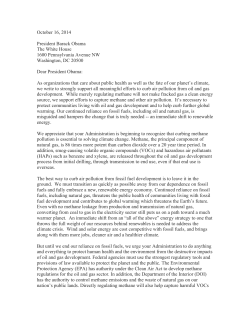
Relative Leakage [%]
EPA Petroleum
(Petron et al., 2012)
EPA Natural Gas
Uintah
(Karion et al., 2013)
Denver-Julesburg
Marcellus
(Caulton et al., 2014)
Eagle Ford
Bakken
Eagle Ford
ΔEmission [ktCH4/yr]
Bakken
The observed anomaly increment over
Bakken, Eagle Ford, and Marcellus is
20
attributed to increases of methane
emissions, arising from the expanded
1500
hydraulic fracturing and increased oil
15
and gas production over the intervening years, because the hot spot areas
1000
are broadly consistent with well posi10
tions and wind direction diﬀerences
between both periods. Other poten500
tial anthropogenic emission sources,
5
such as emissions from agriculture
(e.g., enteric fermentation in live0
0
stock), were temporally constant to a
ﬁrst-order approximation [U.S. EnvironFigure 7. Estimated methane emissions are shown for the targeted regions
Bakken in light brown, and Eagle Ford in dark brown. Shown are absolute
mental Protection Agency, 2013] and
emission increase (2009–2011 relative to 2006–2008) in the left panel, and the
cancel out in the diﬀerence. Wetland
leakage rate relative to production in the right panel, in each case together with
emissions are assumed to vary only
the 1𝜎-uncertainty ranges. For comparison, leakage estimates from previous
studies in Marcellus (2012) [Caulton et al., 2014], Uintah (2012) [Karion et al.,
slightly between both periods, which
2013], and Denver-Julesburg (2008) [Pétron et al., 2012] (yellow, blue, and
is supported by inverse modeling
magenta) are shown together with the EPA bottom-up inventory estimates for
results suggesting no increase in the
natural gas and petroleum systems (2011) [U.S. Environmental Protection Agency,
2014] (grey) in the right panel.
Northern Hemispheric extra-tropics
between the periods [Bergamaschi
et al., 2013]. Additionally, ﬂuxes from wetlands are much smaller than anthropogenic sources in the United
States [Miller et al., 2013] and wetland extent does not match the observed enhancement patterns well, as
concluded from the Kaplan wetland inventory [Bergamaschi et al., 2007].
2000
The production growth (sum of oil and gas) during the analyzed time periods (2009–2011 relative to
2006–2008) was about 250 kBOE/d (BOE = barrel of oil equivalent) for the Bakken [Canadian National
Energy Board, 2011; U.S. Energy Information Administration, 2014a] and 150 kBOE/d for the Eagle Ford [U.S.
Energy Information Administration, 2014a] formation. These values are based on gross production including not marketed natural gas. The emitted CH4 mass estimated from the satellite data is converted to
cubic feet natural gas by using the ideal gas law assuming standard conditions (T = 288.15 K, p = 1013.25
hPa) and a CH4 content of 93% in natural gas [U.S. Environmental Protection Agency, 2013] with a realistic
methane volume fraction range of 0.87–0.99 for high caloric gas. By converting the obtained emission
estimate in cft/yr subsequently to kBOE/d, the following leakage-production ratios in terms of energy
content result: 10.1% ± 7.3% for Bakken and 9.1% ± 6.2% for Eagle Ford. The estimated absolute emission
increases and leakage rates relative to production for the analyzed formations are shown in Figure 7.
5. Discussion
The derived leakage ratios are considerably larger than the bottom-up estimates of 1.2% and 0.7% for
natural gas and petroleum systems [U.S. Environmental Protection Agency, 2014]. Taking the associated
uncertainties into account, methane emissions from energy production of both target formations are
likely underestimated (88% probability) in current bottom-up inventories. The top-down leakage estimates for the two regions exceed the threshold value of 3.2% required for immediate climate beneﬁt
[Alvarez et al., 2012]. This limit assumed switching from coal to natural gas for energy generation, but
production in the analyzed formations is a mixture of gas and oil with Bakken being dominated by oil
production. As oil produces more CO2 per unit of energy than natural gas (140%) [U.S. Energy Information Administration, 2011], the threshold value must thus be further reduced and probably declines below
the lower bound of the 1𝜎-uncertainty-range of the derived leakage ratio in both cases. In conclusion,
at the current methane loss rates, a net climate beneﬁt on all time frames owing to tapping unconventional resources in the analyzed tight formations is unlikely. Based on the derived leakage estimates, there
does not seem to be any rationale to consider reinvigorating the share of petroleum in total electricity
SCHNEISING ET AL.
© 2014 The Authors.
555
Earth’s Future
10.1002/2014EF000265
generation of the United States, which has decreased to a modest value of 1% in recent years [U.S. Energy
Information Administration, 2014b].
The top-down estimates presented are based on long-term satellite data and complement previous
measurement-based results of other regions largely obtained during short-duration campaigns. Our
leakage estimates are similar to the earlier results (Figure 7): 4.0% (2.3%–7.7%) for the Denver-Julesburg
[Pétron et al., 2012], 8.9% (6.2%–11.7%) for the Uintah basin [Karion et al., 2013], and a possible range of
2.8%–17.3% for the Marcellus shale formation [Caulton et al., 2014]. On the other hand, it seems possible
to reduce methane emissions by adopting new technology, as indicated by considerably lower leak rates
close to the EPA inventory estimate found for selected production sites in the Gulf Coast, Midcontinent,
Rocky Mountain, and Appalachian production regions of the United States [Allen et al., 2013]. This suggests that fugitive emissions vary widely from region to region depending on regulations and production
practices.
In contrast to the methane leak rates reported in the literature, which are deﬁned as total emissions
divided by the total production, the leakages derived here are deﬁned as the ratio of the emission
increase between 2006–2008 and 2009–2011 divided by the production growth between these two
periods. The direct comparison of the diﬀerent rates thus inherently assumes that the added production
between 2006–2008 and 2009–2011 leaks methane at the same rate as the total production. This is
reasonable, because the industrial practices and thus the leak rates are considered to remain virtually
constant between the periods in the analyzed regions. If the leakage in the later period had decreased
relative to the former period, the rate based on the added production would be smaller than the total
production leak rate.
The approach used in this study is optimal for regions such as Bakken, Eagle Ford, or Marcellus, where
drilling productivity began to grow rapidly after 2009. However, it is not optimal to determine estimates for the Denver-Julesburg and Uintah basin for direct comparison, because it quantiﬁes emission
changes between two periods rather than total emissions. The production growth in those two basins
is small for the chosen periods according to the Colorado Oil and Gas Conservation Commission
(http://cogcc.state.co.us/) and the Division of Oil, Gas and Mining of the Utah Department of Natural
Resources (http://oilgas.ogm.utah.gov/). Moreover, the rig count, which has for instance increased signiﬁcantly in the Bakken, Eagle Ford, and Marcellus formations [U.S. Energy Information Administration, 2014a],
has decreased in Colorado and Utah during the analyzed periods (2009–2011 relative to 2006–2008)
[Baker Hughes, 2014]. As a consequence, a signiﬁcant and large methane emission increase is not expected
for the Denver-Julesburg and Uintah basin in the analyzed data set.
The above is also the most likely reason why the enhancement patterns over the Permian basin and
gas-dense Haynesville region are less clear than those of the Bakken and Eagle Ford formations (Figure 4),
despite proliﬁc total production from these regions. The Permian basin is more mature than the younger
plays, Bakken and Eagle Ford, with production and rig count virtually stagnating at high levels, whereas
in Haynesville increasing production is concomitant with decreasing rig count, indicating increasing
production eﬃciency with unknown impact on the emission trend [U.S. Energy Information Administration,
2014a]. One possible reason for this improved eﬃciency is that it pays oﬀ in the long run to invest in new
technologies to reduce yield-decreasing fugitive emissions in natural gas systems, whereas in the tight oil
production leakage of natural gas is typically not of primary interest in terms of proﬁtability, because it is
not the targeted resource itself and only used as an auxiliary agent to provide oil ﬂow.
This is also reﬂected in the fact that a signiﬁcant amount of the total natural gas extracted along with
the oil in Bakken and Eagle Ford is ﬂared or otherwise not marketed because the oil is considered more
valuable or pipeline capacities and processing facilities to capture the gas are too costly. The waste of
natural gas as a direct consequence of insuﬃcient infrastructure is so extensive that both regions stand
out clearly in satellite measurements of nighttime lights from the Visible Infrared Imaging Radiometer
Suite (VIIRS) onboard the Suomi National Polar-orbiting Partnership (NPP) satellite [Miller et al., 2012].
In summary, SCIAMACHY nadir measurements show that anthropogenic CH4 emissions from oil and gas
production can be detected from space and that reported bottom-up leakage estimates are likely underestimated for speciﬁc formations. Further studies are needed to provide tighter constraints on fugitive
SCHNEISING ET AL.
© 2014 The Authors.
556
Earth’s Future
10.1002/2014EF000265
emissions and to investigate to what extent the high leakage rates obtained in this and other recent studies are representative for the entire North American oil and gas producing sector. Accurate evaluation of
the impact and sustainability of unconventional oil and gas production across the globe is essential for the
development of wise environmental and energy policy. Future wide swath imaging satellite instruments
delivering higher spatial resolution, such as TROPOMI [Veefkind et al., 2012] and CarbonSat [Bovensmann
et al., 2010; Buchwitz et al., 2013], a candidate for the eighth Earth Explorer of the European Space Agency
(ESA), or the CarbonSat Constellation, when realized, will signiﬁcantly enhance the current capabilities of
satellite observations. CarbonSat and its constellation are projected to enable monitoring emissions down
to the point-source scale [Velazco et al., 2011]. The better precision and accuracy of these new systems
and concepts will yield time-resolved emission estimates during all stages of basin development to better
identify the processes in the life cycle of oil and gas wells leading to the large methane emissions. Such
future satellite missions, ideally supplemented by frequent aircraft and ground-based measurements,
will provide independent veriﬁcation of bottom-up inventories. This is essential for the reliable and accurate determination of the climate impact of exploiting unconventional energy resources in tight geologic
formations.
Acknowledgments
The research leading to these results
has in part been funded by the
ESA project GHG-CCI, the DLR grant
SADOS, the EU project ACCENT-Plus,
and the University and the State of
Bremen. Russell R. Dickerson was
supported by NASA/AQAST. We
thank ESA and DLR for providing the
SCIAMACHY Level 1 data and the SCIAMACHY calibration team (DLR, SRON,
University of Bremen, ESA, and others)
for continuously improving the quality
of the spectra. We acknowledge the
use of data from the U.S. Energy
Information Administration and the
U.S. Environmental Protection Agency.
We also thank the European Centre
for Medium-Range Weather Forecasts
(ECMWF) for providing the meteorological reanalysis data. Fracking well
positions were obtained from SkyTruth
via http://frack.skytruth.org/frackingchemical-database/. North America
rig counts were provided by Baker
Hughes via http://phx.corporate-ir.
net/phoenix.zhtml?c=79687&p=irolreportsother. The methane data set
used in this study is part of the second
version of the Climate Research
Data Package (CRDP#2) of the ESA
project GHG-CCI and is available from
http://www.esa-ghg-cci.org/.
SCHNEISING ET AL.
References
Allen, D. T., et al. (2013), Measurements of methane emissions at natural gas production sites in the United States, Proc. Natl. Acad. Sci.
U. S. A., 110(44), 17,768–17,773, doi:10.1073/pnas.1304880110.
Alvarez, R. A., S. W. Pacala, J. J. Winebrake, W. L. Chameides, and S. P. Hamburg (2012), Greater focus needed on methane leakage
from natural gas infrastructure, Proc. Natl. Acad. Sci. U. S. A., 109(17), 6435–6440, doi:10.1073/pnas.1202407109.
Baker Hughes (2014), North America rig count. [Available at http://phx.corporate-ir.net/phoenix.zhtml?c=79687&p=irol-reportsother.]
Bergamaschi, P., et al. (2007), Satellite chartography of atmospheric methane from SCIAMACHY onboard ENVISAT: 2. Evaluation based
on inverse model simulations, J. Geophys. Res., 112, D02304, doi:10.1029/2006JD007268.
Bergamaschi, P., et al. (2013), Atmospheric CH4 in the ﬁrst decade of the 21st century: Inverse modeling analysis using SCIAMACHY
satellite retrievals and NOAA surface measurements, J. Geophys. Res., 118(13), 7350–7369, doi:10.1002/JGRD.50480.
Bovensmann, H., J. P. Burrows, M. Buchwitz, J. Frerick, S. Noël, V. V. Rozanov, K. V. Chance, and A. P. H. Goede (1999),
SCIAMACHY—Mission objectives and measurement modes, J. Atmos. Sci., 56, 127–150,
doi:10.1175/1520-0469(1999)056<0127:smoamm>2.0.co;2.
Bovensmann, H., M. Buchwitz, J. P. Burrows, M. Reuter, T. Krings, K. Gerilowski, O. Schneising, J. Heymann, A. Tretner, and J. Erzinger
(2010), A remote sensing technique for global monitoring of power plant CO2 emissions from space and related applications,
Atmos. Meas. Tech., 3(4), 781–811, doi:10.5194/amt-3-781-2010.
Brandt, A. R., et al. (2014), Methane leaks from North American natural gas systems, Science, 343(6172), 733–735,
doi:10.1126/science.1247045.
Buchwitz, M., et al. (2013), Carbon monitoring satellite (CarbonSat): Assessment of atmospheric CO2 and CH4 retrieval errors by error
parameterization, Atmos. Meas. Tech., 6(12), 3477–3500, doi:10.5194/amt-6-3477-2013.
Burrows, J. P., E. Hölzle, A. P. H. Goede, H. Visser, and W. Fricke (1995), SCIAMACHY—Scanning Imaging Absorption Spectrometer for
Atmospheric Chartography, Acta Astronaut., 35(7), 445–451, doi:10.1016/0094-5765(94)00278-t.
Canadian National Energy Board (2011), Tight oil developments in the Western Canada sedimentary basin. [Available at
http://www.neb-one.gc.ca/clf-nsi/archives/rnrgynfmtn/nrgyrprt/l/tghtdvlpmntwcsb2011/tghtdvlpmntwcsb2011-eng.pdf.]
Caulton, D. R., et al. (2014), Toward a better understanding and quantiﬁcation of methane emissions from shale gas development,
Proc. Natl. Acad. Sci. U. S. A., 111(17), 6237–6242, doi:10.1073/pnas.1316546111.
Dee, D. P., et al. (2011), The ERA-Interim reanalysis: Conﬁguration and performance of the data assimilation system, Q. J. R. Meteorol.
Soc., 137(656), 553–597, doi:10.1002/qj.828.
Dils, B., et al. (2014), The Greenhouse Gas Climate Change Initiative (GHG-CCI): Comparative validation of GHG-CCI
SCIAMACHY/ENVISAT and TANSO-FTS/GOSAT CO2 and CH4 retrieval algorithm products with measurements from the TCCON,
Atmos. Meas. Tech., 7(6), 1723–1744, doi:10.5194/amt-7-1723-2014.
Dlugokencky, E. J., et al. (2009), Observational constraints on recent increases in the atmospheric CH4 burden, Geophys. Res. Lett., 36,
L18803, doi:10.1029/2009GL039780.
Draxler, R. R., and G. D. Hess (2010), Description of the HYSPLIT_4 modeling system, NOAA Tech. Memo. ERL ARL-224, NOAA Air
Resources Laboratory, Silver Spring, Md.
Howarth, R. W., R. Santoro, and A. Ingraﬀea (2011), Methane and the greenhouse-gas footprint of natural gas from shale formations,
Clim. Change, 106(4), 679–690, doi:10.1007/s10584-011-0061-5.
Intergovernmental Panel on Climate Change (2013), Climate Change 2013: The Physical Science Basis. Contribution of Working Group I
to the Fifth Assessment Report of the Intergovernmental Panel on Climate Change, edited by T. F. Stocker, D. Qin, G.-K. Plattner, M.
Tignor, S. K. Allen, J. Boschung, A. Nauels, Y. Xia, V. Bex, and P. M. Midgley, Cambridge Univ. Press, Cambridge, U. K.
Jackson, R. B., A. Down, N. G. Phillips, R. C. Ackley, C. W. Cook, D. L. Plata, and K. Zhao (2014), Natural gas pipeline leaks across
Washington, DC, Environ. Sci. Technol., 48(3), 2051–2058, doi:10.1021/es404474x.
Karion, A., et al. (2013), Methane emissions estimate from airborne measurements over a western United States natural gas ﬁeld,
Geophys. Res. Lett., 40(16), 4393–4397, doi:10.1002/GRL.50811.
Kleipool, Q. L., R. T. Jongma, A. M. S. Gloudemans, H. Schrijver, G. F. Lichtenberg, R. M. van Hees, A. N. Maurellis, and R. W. M.
Hoogeveen (2007), In-ﬂight proton-induced radiation damage to SCIAMACHY’s extended-wavelength InGaAs near-infrared
detectors, Infrared Phys. Technol., 50(1), 30–37, doi:10.1016/j.infrared.2006.08.001.
Miller, S. D., S. P. Mills, C. D. Elvidge, D. T. Lindsey, T. F. Lee, and J. D. Hawkins (2012), Suomi satellite brings to light a unique frontier of
nighttime environmental sensing capabilities, Proc. Natl. Acad. Sci. U. S. A., 109(39), 15,706–15,711, doi:10.1073/pnas.1207034109.
Miller, S. M., et al. (2013), Anthropogenic emissions of methane in the United States, Proc. Natl. Acad. Sci. U. S. A., 110(50),
20,018–20,022, doi:10.1073/pnas.1314392110.
© 2014 The Authors.
557
Earth’s Future
10.1002/2014EF000265
Nisbet, E. G., E. J. Dlugokencky, and P. Bousquet (2014), Methane on the rise—Again, Science, 343(6170), 493–495,
doi:10.1126/science.1247828.
Pétron, G., et al. (2012), Hydrocarbon emissions characterization in the Colorado Front Range: A pilot study, J. Geophys. Res., 117(D4),
D04304, doi:10.1029/2011JD016360.
Rigby, M., et al. (2008), Renewed growth of atmospheric methane, Geophys. Res. Lett., 35, L22805, doi:10.1029/2008GL036037.
Schneising, O., M. Buchwitz, M. Reuter, J. Heymann, H. Bovensmann, and J. P. Burrows (2011), Long-term analysis of carbon dioxide
and methane column-averaged mole fractions retrieved from SCIAMACHY, Atmos. Chem. Phys., 11(6), 2863–2880,
doi:10.5194/acp-11-2863-2011.
Schneising, O., et al. (2012), Atmospheric greenhouse gases retrieved from SCIAMACHY: Comparison to ground-based FTS
measurements and model results, Atmos. Chem. Phys., 12(3), 1527–1540, doi:10.5194/acp-12-1527-2012.
Schneising, O., J. Heymann, M. Buchwitz, M. Reuter, H. Bovensmann, and J. P. Burrows (2013), Anthropogenic carbon dioxide source
areas observed from space: Assessment of regional enhancements and trends, Atmos. Chem. Phys., 13(5), 2445–2454,
doi:10.5194/acp-13-2445-2013.
SkyTruth (2013), SkyTruth fracking chemical database. [Available at http://frack.skytruth.org/fracking-chemical-database/frackchemical-data-download.]
U.S. Energy Information Administration (2011), Voluntary reporting of greenhouse gases program, table of carbon dioxide emission
factors for stationary combustion. [Available at http://www.eia.gov/oiaf/1605/coeﬃcients.html.]
U.S. Energy Information Administration (2012), Shale oil maps. Bakken Shale Play, Williston Basin, North Dakota, Montana,
Saskatchewan and Manitoba. [Available at http://www.eia.gov/oil_gas/rpd/shaleoil1.pdf.]
U.S. Energy Information Administration (2013), Technically recoverable shale oil and shale gas resources: An assessment of 137 shale
formations in 41 countries outside the United States. [Available at
http://www.eia.gov/analysis/studies/worldshalegas/pdf/overview.pdf.]
U.S. Energy Information Administration (2014a), Drilling productivity report, July 2014. [Available at http://www.eia.gov/petroleum/
drilling/.]
U.S. Energy Information Administration (2014b), Monthly energy review, July 2014. [Available at http://www.eia.gov/totalenergy/data/
monthly/pdf/mer.pdf.
U.S. Environmental Protection Agency (2012), Inventory of U.S. greenhouse gas emissions and sinks: 1990–2010. [Available at
http://www.epa.gov/climatechange/Downloads/ghgemissions/US-GHG-Inventory-2012-Main-Text.pdf.]
U.S. Environmental Protection Agency (2013), Inventory of U.S. greenhouse gas emissions and sinks: 1990–2011. [Available at
http://www.epa.gov/climatechange/Downloads/ghgemissions/US-GHG-Inventory-2013-Main-Text.pdf and
http://www.epa.gov/climatechange/Downloads/ghgemissions/US-GHG-Inventory-2013-Annexes.pdf.]
U.S. Environmental Protection Agency (2014), Inventory of U.S. greenhouse gas emissions and sinks: 1990–2012. [Available at
http://www.epa.gov/climatechange/Downloads/ghgemissions/US-GHG-Inventory-2014-Main-Text.pdf and
http://www.epa.gov/climatechange/Downloads/ghgemissions/US-GHG-Inventory-2014-Annexes.pdf.]
Veefkind, J. P., et al. (2012), TROPOMI on the ESA Sentinel-5 precursor: A GMES mission for global observations of the atmospheric
composition for climate, air quality and ozone layer applications, Remote Sens. Environ., 120, 70–83, doi:10.1016/j.rse.2011.09.027.
Velazco, V. A., M. Buchwitz, H. Bovensmann, M. Reuter, O. Schneising, J. Heymann, T. Krings, K. Gerilowski, and J. P. Burrows (2011),
Towards space based veriﬁcation of CO2 emissions from strong localized sources: Fossil fuel power plant emissions as seen by a
CarbonSat constellation, Atmos. Meas. Tech., 4(12), 2809–2822, doi:10.5194/amt-4-2809-2011.
Wunch, D., G. C. Toon, J.-F. L. Blavier, R. A. Washenfelder, J. Notholt, B. J. Connor, D. W. T. Griﬃth, V. Sherlock, and P. O. Wennberg
(2011), The total carbon column observing network, Philos. Trans. R. Soc. A, 369, 2087–2112, doi:10.1098/rsta.2010.0240.
SCHNEISING ET AL.
© 2014 The Authors.
558