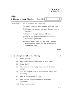
Soil & Tillage Research 77 (2004) 189–202
Estimating the saturated hydraulic conductivity in a spatially
variable soil with different permeameters: a stochastic
Kozeny–Carman relation
Carlos M. Regalado a,∗ , Rafael Muñoz-Carpena b
a
Dep. Suelos y Riegos, Instituto Canario Investigaciones Agrarias (ICIA), Apdo. 60 La Laguna, 38200 Tenerife, Spain
b TREC-IFAS, Agricultural and Biological Engineering Department, University of Florida,
18905 SW 280 St., Homestead, FL 33031-3314, USA
Received 6 July 2003; received in revised form 21 November 2003; accepted 15 December 2003
Abstract
The spatial variability of the saturated hydraulic conductivity (Ks ) of a greenhouse banana plantation volcanic soil was
investigated with three different permeameters: (a) the Philip-Dunne field permeameter, an easy to implement and low cost
device; (b) the Guelph field permeameter; (c) the constant head laboratory permeameter. Ks was measured on a 14 × 5 array of
2.5 m ×5 m rectangles at 0.15 m depth using the above three methods. Ks differences obtained with the different permeameters
are explained in terms of flow dimensionality and elementary volume explored by the three methods. A sinusoidal spatial
variation of Ks was coincident with the underlying alignment of banana plants on the field. This was explained in terms of soil
disturbances, such as soil compaction, originated by management practices and tillage. Soil salinity showed some coincidence
in space with the hydraulic conductivity, because of the irrigation system distribution, but a causal relationship between the
two is however difficult to support. To discard the possibility of an artefact, the original 70 point mesh was doubled by
intercalation of a second 14 × 5 grid, such that the laboratory Ks was finally determined on a 140 points 2.5 m × 2.5 m square
grid. Far from diluting such anisotropy this was further strengthened after inclusion of the new 70 points. The porosity (φ)
determined on the same laboratory cores shows a similar sigmoid trend, thus pointing towards a plausible explanation for such
variability. A power-law relationship was found between saturated hydraulic conductivity and porosity, Ks αφn (r 2 = 0.38),
as stated by the Kozeny–Carman relation. A statistical reformulation of the Kozeny–Carman relation is proposed that both
improved its predictability potential and allows comparisons between different representative volumes, or Ks data sets with
different origin. Although the two-field methods: Guelph and Philip-Dunne, also follow a similar alignment trend, this is not
so evident, suggesting that additional factors affect Ks measured in the field. Finally, geostatistical techniques such as cross
correlograms estimation are used to further investigate this spatial dependence.
© 2004 Elsevier B.V. All rights reserved.
Keywords: Saturated hydraulic conductivity; Philip-Dunne permeameter; Canary Islands; Modified Kozeny–Carman; Banana plant; Stochastic
model
1. Introduction
∗ Corresponding author. Tel.: +34-922-476343;
fax: +34-922-476303.
E-mail addresses: [email protected] (C.M. Regalado),
[email protected] (R. Muñoz-Carpena).
The spatial dependence of the saturated hydraulic
conductivity (Ks ) has been often investigated (Cressie,
1993; Bosch and West, 1998; Moustafa, 2000).
0167-1987/$ – see front matter © 2004 Elsevier B.V. All rights reserved.
doi:10.1016/j.still.2003.12.008
190
C.M. Regalado, R. Muñoz-Carpena / Soil & Tillage Research 77 (2004) 189–202
Geostatistical tools have been used with this purpose (Cressie, 1993), and have helped researchers in
the study of the large variability that Ks often exhibits in soils (Warrick and Nielsen, 1980; Jury et al.,
1991). Additionally, and since the hydraulic conductivity is necessary for predictive hydrological models
(Vachaud et al., 1988; Braud et al., 1995; Moustafa,
2000), its spatial distribution is often required. However the direct determination of Ks requires much
effort and is time consuming, because many measurements are required to represent the intrinsic variation.
Thus indirect methods, based on other more easily
measurable soil properties (such as porosity or texture), are sometimes preferred (Ahuja et al., 1989).
With this purpose in mind either empirically or physically based relationships have been developed to
predict Ks . Among these there is the Kozeny–Carman
equation (Carman, 1937), a power-law that relates Ks
to porosity (φ):
Ks = Aφn
(1)
where A is a proportionality constant and n is a fitting
parameter. In an attempt to improve the predictions
of the above model, some modifications of Eq. (1)
have been proposed which replace φ with the effective porosity, φe , calculated as the saturated water content minus the water content at 33 kPa matric potential
(Ahuja et al., 1984, 1989). Other investigators have
used parameters of the Brooks–Corey or fractal models to replace the exponent n or the proportionality
constant, A in Eq. (1) by measured water retention
parameters (Rawls et al., 1993, 1998; Timlin et al.,
1999). Additionally, relation may also include the specific surface area, Se (m2 m−3 ), such that (Petersen
et al., 1996):
Ks ∝ φn Se−2
(2)
However, the above indirect methods do not always
lead to reliable results (Kutilek and Nielsen, 1994),
thus researchers have resorted to direct measurements
of Ks . Several laboratory (Klute and Dirksen, 1986)
and field direct methods (Amoozegar and Warrick,
1986; Ankeny, 1992; Elrick and Reynolds, 1992) have
been proposed to measure this soil hydraulic property.
Laboratory methods are based on a simple application
of Darcy’s law in one dimension. In some cases, these
have the disadvantage of introducing artefacts because
of soil disturbance (e.g. compaction) and also that the
soil is inhibited from other dominant hydraulic effects
present in the field (capillary effects, other dimensional components, etc.). An example of this method
is the constant head laboratory permeameter (LP)
(Klute and Dirksen, 1986), selected for this work. By
contrast, field methods deal with the soil in natural
conditions and therefore small scale heterogeneities
(structure, texture, flora, fauna, soil composition, etc.)
may contribute to the above one-dimensional flow. It
is thus expected that these field effects will affect the
value and spatial distribution of Ks , but to what extend
this is the case is not well understood. The Guelph
(GP) (Reynolds et al., 1983) and Philip-Dunne (PD)
(Philip, 1993; Gómez et al., 2001; Muñoz-Carpena
et al., 2002) permeameters will be selected in this
work as field methods.
Comparison of the estimations of the hydraulic
conductivity with different methods on a spatial basis
has been poorly investigated in the past (Reynolds
and Zebchuk, 1996), and particularly in relation to the
effect of agricultural practices on the Ks distribution.
Comparisons of laboratory and field Ks methods in
terms of spatial variability are also rare. In addition
studies on the spatial variability of the hydraulic properties of highly micro-aggregated soils, as those of
volcanic origin, are scarce (Romano, 1993; Ciollaro
and Romano, 1995; Zhuang et al., 2000). The intention of this paper is thus two-fold. Firstly the spatial
distribution of Ks in a drip-irrigated volcanic soil banana plantation in the Canary Islands, is compared
using the above three permeameters. In particular we
shall concentrate on the performance of the PD in
predicting the Ks spatial variability (since this is an
easy to implement and low cost but poorly studied
permeameter). Secondly, the predictive capability under field conditions of the Kozeny–Carman relation,
which usually makes use of laboratory determinations is investigated. Modified versions of (1) are also
investigated, in order to improve its predictability
potential and allow for comparison between the different permeameters. By comparing such a relation
with the laboratory and field permeameter Ks , conclusions are drawn about what soil properties may
be determining the spatial structure of the saturated
hydraulic conductivity in the field. Conclusions are
also drawn about the consequences of soil tillage and
management practices on the spatial distribution of
the soil hydraulic properties of a banana plantation.
C.M. Regalado, R. Muñoz-Carpena / Soil & Tillage Research 77 (2004) 189–202
2. Materials and methods
2.1. Soil physical–chemical properties
Vertical undisturbed soil cores were collected at
0.15 m soil depth (top of the core) in stainless steel
rings using a centred hammer driven sampler. The core
dimensions were 0.056 m internal diameter and 0.04 m
high. Water contents in the laboratory for porosity estimation were determined gravimetrically. Field water
contents for the PD measurements (see below) were
obtained with a Trase Time Domain Reflectometry
(TDR) equipment (Soilmoisture Equipment Corp.) using a 0.06 m long three guide probe. A TDR soil specific calibration was carried out since this soil diverges
significantly from Topp’s equation (Regalado et al.,
2003).
Water retention curves (WRC) were determined by
means of Tempe cells on 10 steps of pressure up to
90 kPa suction (ψ) and Richards pressure plates for
these additional pressure steps: 100, 500 and 1500 kPa.
For the description of the retention characteristic, the
model of Brooks and Corey (1964) was used:
 −λ

 ψ
θ − θr
for ψ > ψa
Θ=
=
(3)
ψa

θs − θ r

1
for ψ ≤ ψa
where λ is the pore-size distribution index—a parameter related to the width of the pore-size distribution;
θ, θ s and θ r are the volumetric, saturated and residual
water contents, respectively. Θ is known as the effective saturation; ψa (L) is the matric potential at the air
entry point. Model (3) was fit to the water retention
data with the help of the SHYPFIT program (Durner,
1995).
For the determination of the specific surface, Se ,
the soil was first sieved to 2 mm, dried in vacuum to
constant weight with di-phosphorus pentaoxide and
finally saturated by adsorption in a sulphuric acid
atmosphere (Newman, 1983). We chose this method
instead of others more widely used, such as the
ethyleneglycol method, because it is well known that
the latter overestimates the specific surface in these
soils (Fernandez-Caldas et al., 1982; Gonzales-Batista
et al., 1982).
Na-Amberlite IR-120 (500 ␮m mesh) cation exchange resins were used as dispersing agent for soil
191
texture determination (Bartoli et al., 1991) in air-dried
samples. Particle-size distribution was determined by
the Bouyoucos densimeter method (Gee and Bauder,
1986).
Clay mineralogy was determined by X-ray diffraction in randomly oriented specimens and oriented samples with glycerol and heat treatments (Philips PW
1720) (Whittig and Allardice, 1986).
2.2. Field experimental work
A 850 m2 (33.3 m × 25.5 m) greenhouse dripirrigated banana plantation was selected for sampling and measuring. This was selected because it
is representative of the agricultural practices carried out in the Canary Islands on exportation crops
(mainly bananas and tomatoes). The plot is terraced
with an average soil effective depth of 0.85 m over
basaltic fractured rock. The soil has volcanic origin, clay loam texture (36 ± 6% clay, 21 ± 2%
silt, 43 ± 7% sand) and exhibits andic properties (bulk density < 0.9 g cm−3 , Al0 + 1/2 Fe0 >
2%, phosphate retention > 85%). The soil may
be classified as an Andisol (Armas-Espinel et al.,
2003). The andic character translates into a stable
micro-aggregation and unusual values of soil bulk
density (0.87±0.08 g cm−3 ), porosity (66.42±2.42%)
and specific surface area (200 ± 17 m2 g−1 ). A rectangular regular grid (2.5 m × 5 m) was laid out on
the plot surface yielding 70 grid intersection points
(Fig. 1). A regular grid was chosen since this represents a more efficient sampling scheme (Webster and
Oliver, 1990). The Ks measurement and sampling protocol is described elsewhere (Muñoz-Carpena et al.,
2002).
2.3. Laboratory and field permeameters
Laboratory measurements of Ks were made on a
recirculating constant head permeameter on undisturbed soil cores saturated with calcium sulphate following the procedure described by Klute and Dirksen
(1986).
The Guelph permeameter is a constant head well
permeameter (Reynolds et al., 1983, 1985) consisting on a mariotte bottle that maintains a constant
water level inside a hole augered in the soil. The
simultaneous approach for solving the Richard’s
192
C.M. Regalado, R. Muñoz-Carpena / Soil & Tillage Research 77 (2004) 189–202
Fig. 1. Sampling points and plant distribution of the experimental plot.
based steady-state equation (Philip, 1985; Elrick and
Reynolds, 1992)
2πHi2 Ks + Ci πa2 Ks + 2πHi φm = Ci Qi
(4)
requires at least two different water heads in the same
well. In Eq. (4) φm (m2 s−1 ) is the matric flux potential, Qi (m3 s−1 ) the steady-state flow rate into the
soil, when the steady depth of water in the well is
Hi (m), a (m) the well radius, and Ci is a dimensionless proportionality constant dependent on Hi /a.
The augered wells used in this study were 0.06 m in
diameter, with 0.05 and 0.1 m constant water levels
(Hi ), and C1 = 0.8, C2 = 1.2 (double-head method).
The double-head method may yield negative Ks values due to non-attainment of the steady-state, experimental error, soil profile discontinuity (Elrick et al.,
1989; Elrick and Reynolds, 1992) and ill-conditioning
of the simultaneous equations in Ks and α∗ = Ks/ /φm
(Philip, 1985). To get around negative Ks values, a
single-head procedure has been proposed, whereby a
site estimated α∗ is introduced to avoid the need of
a second ponded head (Elrick et al., 1989). The parameter α∗ may be either obtained from soil textural
characteristics, from the mean α∗ values of all positive
Ks values or by an optimisation procedure (Mertens
et al., 2002). Alternatively, Vieira et al. (1988), have
proposed to recompute the anomalous Ks values (i.e.
φm < 0, α∗ < 1 m−1 , α∗ > 100 m−1 ) arising from
the double-head method, making use of the conductivity values obtained from the Laplace solution, KL
(which neglects the capillarity forces in the soil) and
the “correct” Ks values, Ks∗ , via the empirical relation
γ
Ks∗ = βKL . The fitting parameters β and γ are obtained from the log–log plot of Ks∗ versus KL .
The Philip-Dunne permeameter consists of a tube
of internal radius ri = 0.018 m, vertically inserted to
a certain depth into a soil borehole with zero gap, and
then filled with water up to a height h0 = 0.30 m at
time t = 0. During infiltration, the times when the
pipe is half full (tmed at h = h0 /2) and empty (tmax at
h = 0) are recorded, along with soil moisture at the
beginning (θ 0 ) and at the end of the test (θ 1 ). To obtain
the value of Ks with the PD, the Philip (1993) analysis
makes use of a simplification whereby the disk-shaped
water supply surface is replaced by a spherical water
front of equal area, i.e. of radius r0 = ri /2. If R = R(t)
is the soil wetted bulb radius from the water supply at
time t, then the following differential equation holds
ψf + h0 + π2 /8 R3 − r03
π2 R(R − r0 ) dR
(5)
=
−
8r0 Ks
dt
θ
3r02
C.M. Regalado, R. Muñoz-Carpena / Soil & Tillage Research 77 (2004) 189–202
subjected to the initial condition R(0) = r0 , where
ψf (=α∗−1 ) is the suction at the wetting front and
θ =θ1 −θ0 . Eq. (5) may be integrated to give the temporal variations of the wetted radius and water depth
(Philip, 1993). Making use of the two-measured times,
tmed and tmax and the increment in soil moisture content, θ, the values of Ks and ψf can be computed
(De Haro et al., 1998; Appendix A in Muñoz-Carpena
et al., 2002).
2.4. Statistics
Standard statistics was carried out with SYSTAT 10
(SPSS Inc., 2000) and spatial statistics was performed
with VARIOWIN 2.21 (Pannatier, 1996).
3. Results and discussion
3.1. Statistical results
The saturated hydraulic conductivity was approximately described by a log-normal probability distribution for the three permeameters (Muñoz-Carpena
et al., 2002). Probability plots showed surface area,
porosity and the α∗ parameter to be also closely
log-normally distributed (results not shown). Mean
values of Ks for the different methods are summarised
in Table 1. The LP-Ks (27.90 × 10−4 cm s−1 ) is
Table 1
Mean Ks values (cm s−1 ) ± standard deviation (S.D.) for the laboratory, Philip-Dunne and Guelph permeameters, with the two-head,
Laplace, Vieira and 0.05, 0.10 m one-head methods
Permeameter
Method
Mean Ks ±
S.D. (×104 )
Guelph (GP)
Two-head
Laplace
Vieira
One-head (0.10 m)
One-head (0.05 m)
One-head (0.10 m,
α∗ = 0.12)
One-head (0.10 m,
α∗ = 0.36)
12.07
10.24
6.72
7.77
5.24
5.94
Laboratory (LP)
Klute and Dirksen
(1986)
27.90 ± 2.82
Philip-Dunne (PD)
De Haro et al. (1998)
87.30 ± 4.95
±
±
±
±
±
±
8.74
5.04
2.61
4.24
2.86
3.36
8.42 ± 4.77
193
placed in between the PD and GP. Differences between field and laboratory methods are well known
in the literature (see also discussion below). The
PD gives the highest values (8.73 × 10−3 cm s−1 )
while the Guelph permeameter shows a decreasing trend from the two-head (12.07 × 10−4 cm s−1 ),
Laplace (10.24 × 10−4 cm s−1 ), 0.10 m one-head
(7.77 × 10−4 cm s−1 ), Vieira (6.72 × 10−4 cm s−1 )
and 0.05 m one-head (5.24 × 10−4 cm s−1 ) methods.
For the one-head method we used the mean α∗ =
0.22 cm−1 value obtained from the Vieira analysis.
This value for α∗ is placed between α∗ = 0.12 cm−1 ,
proposed for structured clay loamy soils and unstructured sands, and α∗ = 0.36 cm−1 for highly
structured soils and coarse sands, and it is thus consistent with the expected α∗ deducible from textural
soil characteristics (Elrick et al., 1989). The errors
involved by choosing either of these two extreme α∗
values are though small (cf. row 4 with 6 and 7 in
Table 1).
3.2. Spatial distribution of Ks
Fig. 2 depicts the contour plots of the spatial distribution of Ks obtained with the three permeameters:
LP, GP and PD. It can be seen that the LP-Ks follows
a spatial trend that resembles the alignment of banana plants (compare with Fig. 1). Field Ks exhibits
a subtler aligned disposition, which is also smoothed
out because of edge effects that render some high Ks
values. Many factors may be responsible for these differences. Flow dimensionality and the representative
elementary volume are considered here as the two
most relevant.
3.3. Flow dimensionality
Flow dimensionality may be a source of difference among permeameters. Horizontal saturated hydraulic conductivity, Ksh , determinations on a subset
of 10 cores showed significant differences between
Ksh and Ks (mean Ksh = 0.02275 cm s−1 and mean
Ks = 0.00093 cm s−1 ). Laboratory measurements are
mainly prevented from other than one-dimensional
flow components. Thus the faster horizontal water flow component may counteract high vertical
Ks values in those permeameters that explore the
three space dimensions, i.e. field permeameters, and
194
C.M. Regalado, R. Muñoz-Carpena / Soil & Tillage Research 77 (2004) 189–202
Fig. 2. Contour plots of the spatial distribution of porosity and Ks as determined by the LP, GP and PD. x–y-axes labels denote distance
(m). The grey scale represents Ks (cm s−1 ) or porosity (cm3 cm−3 ) values.
therefore smooth out spatial Ks differences. Basak
(1972) found that the hydraulic conductivity of kaolinite was greater in the horizontal than in the radial
direction. X-ray diffraction shows that the dominant
mineralogical phases of the studied soil are allophane and halloysite and a minor phase of illite.
Halloysite consists of elementary layers of kaolinite and water. Hence the anisotropic orientation of
kaolinite may explain the large horizontal conductivity (Basak, 1972), and thus the differences between
permeameters. Although the Philip-Dunne permeameter assumes a three-dimensional spherical flow,
this is a simplification made for mathematical convenience (see above). The “true” flow is initially
one-dimensional and approaches three dimensionality
only when h0 − h = 4θ0 r0 (Philip, 1993). Such initial disk-shape one-dimensionality may be reinforced
because of the orientation of clay particles, and thus
yield large PD-Ks values.
3.4. Representative elementary volume
The different volume explored by the three permeameters: 2 × 10−3 m3 for the PD and 4 × 10−3 m3 for
the GP versus 1×10−4 m3 for the LP (Muñoz-Carpena
et al., 2002), may be also an important factor that explains Ks differences, since a larger volume averages
over more heterogeneities, and this results in a lower
variability in the field methods. This agrees with the
values obtained for the coefficient of variability, which
is highest for the LP (101%), followed by the PD
(56%) and GP (56 and 38% for the single-head and
Vieira Ks , respectively).
3.5. Other factors: permeameter assumptions, field
heterogeneity, initial water content
Even taking these considerations into account comparison between different methods is difficult because
C.M. Regalado, R. Muñoz-Carpena / Soil & Tillage Research 77 (2004) 189–202
of underlying assumptions, different response of the
permeameter to soil conditions, etc. (Bouma, 1983).
Additionally, field specific heterogeneities (flora,
fauna, etc.) may also mask Ks differences within
a close neighbourhood. Although soil initial water
content, θ i , was not monitored prior to the GP measurements, no correlation was observed between θ i
and PD-Ks , contrary to Reynolds and Zebchuk (1996)
who found that antecedent water content was slightly
correlated with GP-Ks . It is the increment in water
content before and after the test has been performed,
and not the antecedent water content, what is related
to the PD-Ks (see Eq. (5)). Assuming that both PD-Ks
and GP-Ks are somehow related, the same would be
expected for the Guelph permeameter.
Some low suction values at the wetting front were
coincident with large porosities, but with no clear spatial structure (results not shown). This may be due to
the large uncertainty implicit in the estimation of α∗
(Mertens et al., 2002).
3.6. Banana plants versus Ks
Several hypotheses may be explored in order to explain the coincidence of banana plants and LP-Ks .
First, the banana root system (exploring the top 0.30 m
of the soil) may affect the surrounding soil physical
properties. In fact the annual selection of shoots from
the mother banana plant yields a spatial “rotation” of
plants. This may explain that the matching of plants
and LP-Ks is not perfect.
Secondly, localised drip fertigation may modify the
hydraulic conductivity of the soil in the neighbourhood of plants. For example Dorel et al. (2000), found
that surface desiccation of an Andosol planted with
bananas, led to a significant soil shrinkage that affected its hydraulic properties. The accumulation of
salts around the wetting bulb may also exert chemical effects upon the soil constituents, which result in
alteration of its hydraulic properties (Bresler et al.,
1984 and references therein). However, the magnitude of this effect depends not only upon the salt
source but also upon the nature of the soil materials.
Armas-Espinel et al. (2003) found that low Ks in volcanic soils was associated with high (Na+Mg)/Ca ratios and low electrical conductivity (EC) values, which
they attributed to an increase in swelling pressure. Additionally, excess sodium in low salinity conditions
195
will decrease hydraulic conductivity through dispersion of fine clay materials. Fig. 3 shows the surface
plot of LP-Ks , EC and exchangeable sodium percentage (ESP) of the soil saturation extract. It can be
observed an almost exact matching between EC and
ESP and certain coincidence of LP-Ks and the salinity status. A cross correlogram analysis (see Section
3.9) shows that EC–ESP correlation is high 0.773 (covariance σ = 7.96 × 10−2 ). According to Emerson
(1977), soil swelling pressure raises with increasing
ESP and decreasing EC. Therefore a swelling mechanism seems unlikely to explain the spatial distribution of Ks , since high values of ESP would be
counterbalanced by high salinity conditions (Wagenet
and Bresler, 1983) (Fig. 3). Salinisation and sodification, induced by irrigation with low quality waters
and intensive fertilisation, is frequent in cultivated
soils from the Canary Islands—mean CE in this soil
is 4.70 dS m−1 . Also, physical properties of clayey
soils can be strongly affected by amorphous materials and oxy-hydroxides of iron and aluminium. Such
andic materials induce strong aggregation and impart favourable structural properties such as reduced
swelling (El-Swaify, 1975). It is suggested that the
spatial coincidence of soil salinity with the hydraulic
conductivity, is an artefact of the irrigation system distribution. This is also in agreement with Bresler et al.
(1984) who found that soil salinity only accounted for
10–15% of the spatial variability of Ks in two selected
agricultural fields.
Finally field management practices and tillage may
introduce soil disturbances, such as soil compaction,
and this by turn may affect Ks . Dorel et al. (2000)
showed that soil hydraulic conductivity was drastically reduced in the compacted layers of a mechanised
banana plantation, and that soil tillage increased the
mean Ks . Also Moustafa (2000) found that the spatial
dependence of Ks was correlated with the agricultural
practices of field soils in Egypt.
3.7. Ks versus porosity
From the above discussion it follows that both heterogeneous desiccation and compaction may be responsible for the spatial distribution of Ks , probably
because these affect soil structure. Dorel et al. (2000)
showed that the hydraulic effects of both mechanisation and desiccation on an Andosol banana plantation
196
C.M. Regalado, R. Muñoz-Carpena / Soil & Tillage Research 77 (2004) 189–202
Fig. 3. Surface plots of the laboratory Ks , electrical conductivity (EC) and exchangeable sodium percentage (ESP) of the soil saturation
extract.
C.M. Regalado, R. Muñoz-Carpena / Soil & Tillage Research 77 (2004) 189–202
were due to changes in soil porosity. The hypothesis
of soil compaction would be also consistent with the
preferential horizontal orientation of clays in this soil
(see above), since compacted clays will be more oriented than non-compacted clays (Al-Tabaa and Wood,
1987). Basak (1972) found that the vertical hydraulic
conductivity of kaolinite was more sensitive to the void
ratio (volume of voids/volume of solid) than the radial
hydraulic conductivity. Thus LP-Ks will be more sensitive to differences in soil compaction than the field
methods.
The Kozeny–Carman relation (1) was first tested as
a plausible explanatory model for the distribution of
Ks , since also Fig. 2 already points in this direction.
Porosity values, obtained on the same cores that LP-Ks
were determined, show a power-law relationship of
the form: Ks = 5 × 10−33 φ16.27 (r 2 = 0.38) as stated
in (1). There exists the possibility that such a correlation between LP-Ks and φ may be biased because
soil cores were placed inside the lab-permeameter in
groups of 10 consecutive samples. In order to discard such an artefact, a second 70 grid point mesh
was intercalated in between the first one, such that
the laboratory Ks and porosity were finally determined
on a 2.5 m × 2.5 m square grid. Additionally, in such
a square grid the maximum distance between neighbour sampling points is maximised. Thus unrepresentation and redundancy of some areas is minimised
(Webster and Oliver, 1990). The order of introduction
of the new soil cores in the LP was randomised to
197
further discard a possible bias in the Ks determination.
Far from diluting such anisotropy, this was further
strengthened, thus suggesting a plausible origin for the
spatial distribution of the laboratory conductivity data
(Fig. 4).
Comparison of measured and predicted Ks figures
shows that in general predicted Ks differences have
been smoothed out. High LP-Ks values on the left edge
have been almost erased and some of the LP-Ks “hot
spots” in the plants middle lines have also disappeared.
All this indicates that not only porosity but also some
other factors may affect the value of Ks .
In an attempt to look for such factors responsible for the Ks spatial dependence, we tried a modified Kozeny–Carman relation proposed by Ahuja et al.
(1984), where φ is replaced by the effective porosity,
φe is calculated as the saturated water content minus
the water content at 33 kPa matric potential. Additionally, the relation
Ks ∝ φe3−λ
(6)
where the exponent n in (1) has been replaced by the
λ parameter of the Brooks–Corey model (3), was also
investigated. A linear relation in the log–log space was
found between Ks versus φe (r 2 = 0.36), thus confirming the model of Ahuja et al. (1984). However for
model (6) we did not find a simple law of proportionality Ks versus φe3−λ , but an exponential dependence,
although with large data dispersion (r 2 = 0.25). This
result suggests the possibility of a relation of the form
Fig. 4. Contour plots of the spatial distribution of measured vs. estimated LP-Ks as predicted by relation Ks = 5 × 10−33 φ16.268 . White
crosses correspond to sampling points. The grey scale represents Ks values (cm s−1 ). x–y-axes labels denote distance (m).
198
C.M. Regalado, R. Muñoz-Carpena / Soil & Tillage Research 77 (2004) 189–202
(Rawls et al., 1993; Timlin et al., 1999)
Ks = B(λ, ψa )φn
(7)
By plotting B, calculated as Ks /φn for fix n = 2.5,
against λ or ψa , we identified a possible functional
dependence of this parameter on the air entry potential index. Such dependence is highly non-linear,
Bα exp(ψa ), although very scattered, r 2 = 0.16
(Regalado and Muñoz-Carpena, 2001). Furthermore,
considering the coefficient B either a function of ψa
alone or a combination of λ and ψa in (7), did not
significantly improved the predictions of Ks versus φe .
3.8. A stochastic Kozeny–Carman relation
In this and previous studies (Messing and Jarvis,
1990; Timlin et al., 1999; Zhuang et al., 2000) the fitting results obtained with the Kozeny–Carman equations (1) and (2) are usually poor. In order to improve
its predictability potential, the modified versions (6)
and (7) have been proposed, although still the scattering is remarkable (Ahuja et al., 1984, 1989). The
Kozeny–Carman relation assumes a deterministic
point-to-point relationship between Ks and some soil
physical property, such as porosity or surface area.
However this hypothesis may not be valid if for example physical properties are determined on samples
close to, but from a different location where Ks has
been measured, or if the volume that such properties
(e.g. surface area) refer to differs significantly from
the representative Ks volume, and thus averaging
Se over the whole Ks volume may not be realistic.
This may also explain the lack of accuracy of the
above expressions. Hence a statistical reformulation
of the Kozeny–Carman equation would be desirable,
whereby pairs of observation frequencies replace
point-to-point correlations. The following stochastic
form of (2) is thus proposed
P(Ks ) ∝ A · ℵ(φ, µ1 , σ1 )p ℵ(Se , µ2 , σ2 )q
(8)
where P(Ks ) is the cumulative frequency of Ks ; ℵ(·)
the normal cumulative distribution function (CDF)
of porosity and surface area, respectively, with shape
parameters µi , σ i ; A, p, q are the fitting parameters.
Normal CDFs were first fitted to the cumulative frequencies of φ and Se . Obtained parameters µi and σ i
are 0.662, 0.026 (r2 = 0.996) and 172.50, 15.24 (r2 =
Fig. 5. Agreement between experimental laboratory constant head
Ks data and the proposed stochastic Kozeny–Carman equation (8).
0.998), respectively. These were then substituted into
(8) and a least square fitting procedure was used to
estimate the parameters A = 1.065, p = 0.434 and
q = 0.552 from the cumulative frequencies of LP-Ks
(r 2 = 0.999) (Fig. 5).
The same procedure followed above for the laboratory Ks data may be pursued with the field
determinations. As already discussed, a statistical representation of the Kozeny–Carman equation (1), does
not preclude a point-to-point relationship between the
fitted variables, and thus the porosity data obtained in
the laboratory cores may be used to predict the frequency of Guelph and Philip-Dunne measurements.
The following statistical form of (1) was investigated
P(Ks ) = A · ℵ(φ, µ, σ)p
(9)
where P(Ks ) is the cumulative frequency of Ks and A
is a fitting proportionality constant. Good fit was obtained with the PD data (µ = 0.662, σ = 0.026, A =
0.994, p = 0.992, r2 (observed versus predicted) =
0.987), but a poorer regression (cf. Fig. 6a and b)
was achieved with the GP measurements (µ =
0.643, σ = 0.009, A = 0.966, p = 0.956,
r 2 (observed versus predicted) = 0.966), thus indicating that either the Guelph method is more sensitive to
errors in the porosity estimates or it is more affected
by other soil properties not considered in (9) (Fig. 6).
The values of the constant A and the power p in (9)
are very close to unity, thus field frequencies may
C.M. Regalado, R. Muñoz-Carpena / Soil & Tillage Research 77 (2004) 189–202
199
Fig. 6. Agreement between experimental data and the proposed stochastic Kozeny–Carman equation (9) for the field Guelph, GP-Ks (a)
and Philip-Dunne, PD-Ks (b) permeameter data sets.
be estimated from porosity values without additional
fitting. Furthermore the shape parameters of the PD
distribution are the same than the ones obtained for
the porosity CDF (see above), indicating that both
follow a similar trend of occurrence even though a
point-to-point relationship may not be established.
3.9. Geostatistical analysis
Geostatistics is the name proposed for a method
of spatial analysis that makes predictions from a
sample data, whose relative spatial locations are
known. In geostatistics it is required that the expectation of a random measurement made at location
x, is constant. This hypothesis is known as the stationarity assumption, and it is often overlooked by
researchers who proceed directly to applying geostatistical tools. By comparing the median versus the
squared inter-quartile range (a measure of the data
spreading independent of symmetry) for different data
transformations, one may find a suitable symmetrising and variance stabilising transformation (Cressie
and Horton, 1987). The log-transformation was found
to satisfy both criteria, i.e. (1) it made the data symmetric, and (2) it straightened out the data such that
variation is no longer a function of location (Regalado
and Muñoz-Carpena, 2001).
In order to quantify spatial correlations between
variables, we assessed the correlation between adjacent log-transformed porosity and LP-Ks observations. The plot of the estimated correlation coefficient
Fig. 7. Directional experimental cross correlograms of log-porosity
vs. log-LP-Ks . (a) Horizontal (west-east) direction; (b) vertical
(south-north) direction. Numbers on empty circles indicate number
of pair comparisons used to compute the correlation coefficient.
200
C.M. Regalado, R. Muñoz-Carpena / Soil & Tillage Research 77 (2004) 189–202
of log-porosity versus log-LP-Ks as a function of the
separation distance, the so called experimental cross
correlogram, is shown in Fig. 7. Directional correlograms in both the horizontal (west-east) direction
(Fig. 7a) and vertical (south-north) direction (Fig. 7b)
are plotted. It may be observed that although horizontal correlation decreases up to 22.5 m, beyond this
an increasing correlation tendency may be observed
with the separation distance (an effect previously referred to as the lag effect). The same occurs in the
vertical direction for separation distances greater than
15 m. However in general correlation is greater at
shorter distances, while large-range correlations are
supported by a smaller number of pair comparisons
(cf. numbers shown in graph).
4. Summary and conclusions
The saturated hydraulic conductivity is often required for hydrological studies and it is either laboratory or field measured, or it is deduced from other more
easily measurable physical soil properties. However,
not very often its spatial structure is investigated by
comparing different estimation methods. Significant
differences observed between Ks measurements may
be partly explained in terms of flow dimensionality
and representative elementary volumes, and may be
worsened because preferential flow in the horizontal
component, originated by orientation of clay particles
in this soil. The results shown in this paper indicate that
although soil (effective) porosity may be an underlying
process determining Ks distribution, field effects may
smooth out this dependence such that this is no longer
detectable. We may thus conclude that the spatial variability of Ks is not an easily distinguishable result of
soil porosity or water retention characteristics. This is
also affected by other components of the soil (e.g. clay
content, degree of aggregation), especially under field
conditions, or by the experimental design (e.g. measurement technique). All these factors are difficult to
detect if comparisons between different permeameters
are not performed or Ks measurements are restricted
to laboratory determinations. This may also limit the
field applicability of indirect Ks estimation methods
of the kind of the Kozeny–Carman model, which usually makes use of laboratory determinations, thus neglecting other field factors more relevant to the soil in
natural conditions. A modified Kozeny–Carman equation defined in statistical terms may overcome these
limitations, allowing comparisons between different
representative volumes or Ks data sets with different
origin. This is also a rather convenient reformulation,
amenable for stochastic modelling or Monte-Carlo
simulations of the spatial variability of hydraulic
properties, whereby locally defined parameter values
are replaced by probability distribution functions of
parameters (Braud et al., 1995; Vachaud et al., 1988),
and thus this deserves further investigation.
Processes promoting soil degradation as surface
desiccation and soil compaction, induced by tillage
and localised irrigation, may be responsible for the
anisotropy of Ks . Soil salinity showed some coincidence in space with the hydraulic conductivity, because of the irrigation system distribution, but a causal
relationship between the two is discarded, since high
values of exchangeable sodium are counterbalanced
by high salinity conditions and andic materials that
impart favourable structural properties, such as reduced swelling. This had not been detected if detailed
information about soil mineralogy and chemical properties had not been available, and we had thus arrived
to erroneous conclusions about the origin of the spatial distribution of Ks . Such considerations of both
spatial dependence and measuring technique should
very much be taken into account in future studies
intending to make use of a single (mean) effective
value of the saturated hydraulic conductivity.
Acknowledgements
This work has been supported by the Florida
Agricultural Experiment Station Journal Series No.
R-09021, a Project Grant and Postdoctoral Fellowship from the Spanish INIA-National R & D Program
(Project SC99-024-C2-1) and the European Union
COST Action 622. The authors would like to thank
Dr. J. Jawitz from the Soil and Water Department,
University of Florida, for his careful reading and
revision of the manuscript.
References
Ahuja, L.R., Naney, J.W., Green, R.E., Nielsen, D.R., 1984.
Macroporosity to characterize spatial variability of hydraulic
C.M. Regalado, R. Muñoz-Carpena / Soil & Tillage Research 77 (2004) 189–202
conductivity and effects of land management. Soil Sci. Soc.
Am. J. 48, 699–702.
Ahuja, L.R., Cassel, D.K., Bruce, R.R., Barnes, B.B., 1989.
Evaluation of spatial distribution of hydraulic conductivity using
effective porosity. Soil Sci. 148, 404–411.
Al-Tabaa, A., Wood, D.M., 1987. Some measurements of the
permeability of kaolin. Géotechnique 37, 499–503.
Amoozegar, A., Warrick, A.W., 1986. Hydraulic conductivity of
saturated soils: field methods. In: Klute, A. (Ed.), Methods of
Soil Analysis. Part 1. Physical and Mineralogical Methods, 2nd
ed. Agron. Monogr. 9. ASA, Madison, WI, pp. 735–770.
Ankeny, M.D., 1992. Methods and theory for unconfined
infiltration measurements. In: Topp, G.C., Reynolds, W.D.,
Green, R.E. (Eds.), Advances in Measurements of Soil Physical
Properties: Bringing Theory into Practice. SSSA Spec. Publ.
30. SSSA, Madison, WI, pp. 123–141.
Armas-Espinel, S., Hernández-Moreno, J.M., Muñoz-Carpena,
R., Regalado, C.M., 2003. Physical properties of “sorriba”cultivated volcanic soils from Tenerife in relation to andic
diagnostic parameters. Geoderma 117, 297–311.
Bartoli, F., Burtin, G., Herbillon, A., 1991. Disaggregation and clay
dispersion of Oxisols: Na resin, a recommended methodology.
Geoderma 49, 301–307.
Basak, P., 1972. Soil structure and its effects on hydraulic
conductivity. Soil Sci. 114, 417–422.
Bosch, D.D., West, L.T., 1998. Hydraulic conductivity variability
for two sandy soils. Soil Sci. Soc. Am. J. 62, 90–98.
Bouma, J., 1983. Use of soil survey data to select measurement
techniques for hydraulic conductivity. Agric. Water Manage. 6,
177–190.
Braud, I., Dantas-Antonino, A.C., Vauclin, M., 1995. A stochastic
approach to studying the influence of the spatial variability
of soil hydraulic properties on surface fluxes. J. Hydrol. 165,
283–310.
Bresler, E.G., Dagan, G., Wagenet, R.J., Laufer, A., 1984.
Statistical analysis of salinity and texture effects on spatial
variability of soil hydraulic conductivity. Soil Sci. Soc. Am. J.
48, 16–25.
Brooks, R.H., Corey, A.T., 1964. Hydraulic Properties of Porous
Media. Hydrology Paper 3. Colorado State University, Fort
Collins, CO, pp. 1–27.
Carman, P.C., 1937. Fluid flow through granular beds. Trans. Inst.
Chem. Eng. 15, 150–166.
Ciollaro, G., Romano, N., 1995. Spatial variability of the hydraulic
properties of a volcanic soil. Geoderma 65, 263–282.
Cressie, N.A.C., 1993. Applications of geostatistics. In: Statistics
for Spatial Data. Wiley Series in Probability and Mathematical
Statistics. Wiley, New York, pp. 211–276.
Cressie, N.A.C., Horton, R., 1987. A robust-resistant spatial
analysis of soil water infiltration. Water Resour. Res. 23, 911–
917.
De Haro, J.M., Vanderlinden, K., Gómez, J.A., Giráldez, J.V., 1998.
Medida de la conductividad hidráulica saturada. In: González,
A., Orihuela, D.L., Romero, E., Garrido, R. (Eds.), Progresos
en la Investigación de la Zona No Saturada, Collectanea, vol.
11. Universidad de Huelva, Spain, pp. 9–20.
201
Dorel, M., Roger-Estrade, J., Manichon, H., Delvaux, B., 2000.
Porosity and soil water properties of Caribbean volcanic ash
soils. Soil Use Manage. 16, 133–140.
Durner, W., 1995. SHYPFIT 0.24, User’s Manual. Research
Report 95.1. Department of Hydrology, University of Bayreuth,
Germany.
Elrick, D.E., Reynolds, W.D., 1992. Infiltration from constant-head
well permeameters and infiltrometers. In: Topp, G.C., Reynolds,
W.D., Green, R.E. (Eds.), Advances in Measurements of Soil
Physical Properties: Bringing Theory into Practice. SSSA Spec.
Publ. 30. SSSA, Madison, WI, pp. 1–24.
Elrick, D.E., Reynolds, W.D., Tan, K.A., 1989. Hydraulic
conductivity measurements in the unsaturated zone using
improved well analyses. Ground Water Monit. Rev. 9, 184–193.
El-Swaify, S.A., 1975. Changes in the physical properties of soil
clays due to precipitated aluminium and iron hydroxides. I.
Swelling and aggregate stability after drying. Soil Sci. Soc.
Am. Proc. 39, 1056–1063.
Emerson, W.W., 1977. Physical properties and soil structure.
In: Russel, J.S., Greacen, E.L. (Eds.), Soil Factors in
Crops Production in a Semiarid Environment. University of
Queensland Press, St. Lucia, Qld, pp. 78–104.
Fernandez-Caldas, E., Tejedor-Salguero, M.L., Quantin, P., 1982.
Suelos de regiones volcánicas. Tenerife, Islas Canarias.
Colección Viera y Clavijo. IV. Secretariado de publicaciones
de la Universidad de La Laguna, CSIC (in Spanish).
Gee, G.W., Bauder, J.W., 1986. Particle-size analysis. In: Klute,
A. (Ed.), Methods of Soil Analysis. Part 1. Physical and
Mineralogical Methods, 2nd ed. Agronomy 9. ASA/SSSA,
Madison, WI, pp. 383–411.
Gómez, J.A., Giráldez, J.V., Fereres, E., 2001. Analysis of
infiltration and runoff in an Olive Orchard under no-till. Soil
Sci. Soc. Am. J. 65, 291–299.
Gonzales-Batista, A., Hernández-Moreno, J.M., Fernández-Caldas,
E., Herbillón, A.J., 1982. Influence of silica content on the
surface charge characteristics of allophanic clays. Clays Miner.
30, 103–110.
Jury, W.A., Gardner, W.R., Gardner, W.H., 1991. Soil Physics.
Wiley, New York.
Klute, A., Dirksen, C., 1986. Hydraulic conductivity and
diffusivity: laboratory methods. In: Klute, A. (Ed.), Methods
of Soil Analysis. Part 1. Physical and Mineralogical Methods,
2nd ed. Agron. Monogr. 9. ASA, Madison, WI, pp. 687–734.
Kutilek, M., Nielsen, D.R., 1994. Soil Hydrology. CREMLINGENDestedt: CATENA-Verlag, Catena.
Mertens, J., Jacques, D., Vanderborght, J., Feyen, J., 2002.
Characterisation of the field-saturated conductivity on a
hillslope: in situ single ring pressure infiltrometer measurements. J. Hydrol. 263, 217–229.
Messing, I., Jarvis, N.J., 1990. Seasonal variation in field-saturated
hydraulic conductivity in two swelling clay soils in Sweden. J.
Foil Sci. 41, 229–237.
Moustafa, M.M., 2000. A geostatistical approach to optimize the
determination of saturated hydraulic conductivity for large-scale
subsurface drainage design in Egypt. Agric. Water Manage. 42,
291–312.
Muñoz-Carpena, R., Regalado, C.M., Álvarez-Bened´ı, J., Bartoli,
F., 2002. Field evaluation of the new Philip-Dunne permeameter
202
C.M. Regalado, R. Muñoz-Carpena / Soil & Tillage Research 77 (2004) 189–202
for measuring saturated hydraulic conductivity. Soil Sci. 167,
9–24.
Newman, A.C.D., 1983. The specific surface of soils determined
by water sorption. J. Soil Sci. 34, 23–32.
Pannatier, Y., 1996. VARIOWIN: Software for Spatial Data
Analysis in 2D. Springer-Verlag, New York.
Petersen, L.W., Moldrup, P., Jacobsen, O.H., Rolston, D.E., 1996.
Relations between specific surface area and soil physical and
chemical properties. Soil Sci. 161, 9–21.
Philip, J.R., 1985. Approximate analysis of the borehole
permeameter in unsaturated soil. Water Resour. Res. 21, 1025–
1033.
Philip, J.R., 1993. Approximate analysis of falling-head lined
borehole permeameter. Water Resour. Res. 29, 3763–3768.
Rawls, W.J., Brakensiek, D.L., Logsdon, S.D., 1993. Predicting
saturated hydraulic conductivity utilizing fractal principles. Soil.
Sci. Soc. Am. J. 57, 1193–1197.
Rawls, W.J., Gimenez, D., Grossman, R., 1998. Use of soil
texture, bulk density, and slope of the water retention curve to
predict saturated hydraulic conductivity. Trans. ASAE 41, 983–
988.
Regalado, C.M., Muñoz-Carpena, R., 2001. Field spatial variability
of the saturated hydraulic conductivity as measured with three
kinds of permeameters. ASAE Annual International Meeting,
Paper Number 012147, Sacramento, California, USA.
Regalado, C.M., Muñoz-Carpena, R., Socorro, A.R., Hernández
Moreno, J.M., 2003. Time domain reflectometry models as a
tool to understand the dielectric response of volcanic soils.
Geoderma 117, 313–330.
Reynolds, W.D., Elrick, D.E., Clothier, B.E., 1985. The constant
head well permeameter: effect of unsaturated flow. Soil Sci.
139, 172–192.
Reynolds, W.D., Elrick, D.E., Topp, G.C., 1983. A reexamination
of the constant head well permeameter method for measuring
saturated hydraulic conductivity above the water table. Soil Sci.
136, 250–268.
Reynolds, W.D., Zebchuk, W.D., 1996. Hydraulic conductivity
in a clay soil: two measurement techniques and spatial
characterization. Soil Sci. Soc. Am. J. 60, 1679–1685.
Romano, N., 1993. Use of an inverse method and geostatistics
to estimate soil hydraulic conductivity for spatial variability
analysis. Geoderma 60, 169–186.
SYSTAT 10, 2000. http://www.systat.com/products/Systat/. SPSS
Inc.
Timlin, D.J., Ahuja, L.R., Pachepsky, Ya., Williams, R.D.,
Gimenez, D., Rawls, W., 1999. Use of Brooks–Corey
parameters to improve estimates of saturated conductivity from
effective porosity. Soil Sci. Soc. Am. J. 63, 1086–1092.
Vachaud, G., Vauclin, M., Balabanis, P., 1988. Stochastic approach
of soil water flow through the use of scaling factors:
measurement and simulation. Agric. Water Manage. 13, 249–
261.
Vieira, S.R., Reynolds, W.D., Topp, G.C., 1988. Spatial variability
of hydraulic properties in a highly structured clay soil. In:
Proceedings of the Symposium on Validation of Flow and
Transport Models for the Unsaturated Zone, Ruidoso, NM.
Wagenet, R.J., Bresler, E., 1983. Soil salinity effects on the
spatial variability of hydraulic conductivity. United States-Israel
Binational Agricultural Research and Development (BARD)
Fund. Final Report Project No. US-21-79, Bet Dagan, Israel.
Warrick, A.W., Nielsen, D.R., 1980. Spatial variability of soil
physical properties in the field. In: Hillel, D. (Ed.), Applications
of Soil Physics. Academic Press, New York, pp. 319–344.
Webster, R., Oliver, M.A., 1990. Statistical Methods in Soil and
Land Resource Survey. Oxford University Press, New York.
Whittig, L.D., Allardice, W.R., 1986. X-ray diffraction techniques.
In: Klute, A. (Ed.), Methods of Soil Analysis. Part 1. Physical
and Mineralogical Methods, 2nd ed. Agron. Monogr. 9. ASA,
Madison, WI, pp. 331–362.
Zhuang, J., Nakayama, K., Yu, G.R., Miyazaki, T., 2000. Scaling
of saturated hydraulic conductivity: a comparison of models.
Soil Sci. 165, 718–727.