Camp. & Maths. wrrh Appk. Vol. I I, No. 4. pp 335-345.
Printed
in Great
0097-4943185
13.00+ 00
iiJ I985 Pergamon Press Ltd
1985
Britain
FIXED MESH FINITE ELEMENT APPROXIMATIONS
TO A FREE BOUNDARY PROBLEM FOR AN
ELLIPTIC EQUATION WITH AN OBLIQUE
DERIVATIVE BOUNDARY CONDITION
JOHN W. BARRETT?
and CHARLES M. ELLIOTT
Department of Mathematics, Imperial College. London S.W.7.. U.K
(Received June 1984)
Communicated
by J. Tinsley Oden
Abstract-A
method for approximating
the solution of an elliptic equation with an oblique derivative
on a curved boundary using an unfitted finite element mesh is presented and analysed. It is shown that
the method retains the order of accuracy of the fitted mesh finite element method. A similar result is
obtained for a variational inequality. The usefulness of this approach is then demonstrated by using it
to approximate the solution of a free boundary problem on a fixed mesh.
I.
INTRODUCTION
Free boundary problems for Poisson equations, in particular those amenable to variational
inequality techniques, have been widely studied in recent years; see [2, 8, 9, lo]. Frequently
an integral transformation of the dependent variable in the original problem is required in order
to obtain a variational inequality formulation. This integration transforms Dirichlet boundary
conditions into oblique derivative conditions for the transformed variable. A typical problem,
arising in the mathematical modelling of an electrochemical machining process[7], is to find a
curve r defined by ~1 = d(x), x E [-I!,, L], such that
d(-L)
where x E [-L,
satisfying
=
L], d(x) E C[ -L,
d(L)
=
,!,I rl Cx( -f.,
c(O) = c’(0) = 0,
c(L) = Yz <
and a function
u(x. y) E H’(Q)
n =
Y3,
Y3,
{(x, y): -L
>
(l.la)
c(x)
L) and where c(x) E C3[-L,
= Y, < Y3,
c( -L)
C”(X)
r‘l C’(b),
d(x)
>
0,
x
E
(-L,
L.1 is given
(l.lb)
L),
where
c(x) < y < d(x))
< x < L,
and
D = {(x, y): -L
c(x) < y < Y,},
< x < L,
such that
V’u = ;7> 0
u,(x, c(x))
= - 1
u(--L,
y)
and
and
=
u(x, Y,) = 0,
V,(r)
> 0,
UC. y) = U,(?.) > 0,
II
+Supponed
b> S.E.R.C
=
u, =
postdoctoral
u,
= Oonr,
fellowship
u > 0
RF:5830.
4’ E
?’
in
Q,
x E (-L,
(Y,,
Y,),
E (Yz, Y,),
u=OinD\Q.
(l.lc)
L),
(l.ld)
(l.le)
(l.lf)
(l.lg)
336
J. W. B.A.RRETTand C. M.
ELLIOIT
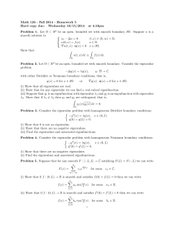
Here VI(.) and Uz(.) are given non-negative functions, which are continuously
differentiable.
satisfying U,(YJ = (/?(Yj) = 0 and CJ;(Y,) = UJ(YI) = - 1: and ;’ is a given positive constant.
The region is depicted in Figure 1 which also defines the open sets f,.
The first equation of (1. Id) is an oblique derivative boundary condition which can be
written as
at4
a\,
+
c’(x)
$ = -(l
+ c’(x)~)’ ? on r,,
(1.2)
where v and 0 are, respectively, the unit inward pointing normal and anticlockwise tangential
vectors to the curve f, at (x, y). Using the fact that u solves a variational inequality, it was
shown[7] that, when the problem is symmetric about .r = 0, there exists a unique solution to
this free boundary problem such that u E W’J’(D) II C’,‘@) for all p E [ 1, x) and i. E (0.
1). Such free boundary problems for Poisson equations with oblique derivative conditions on
fixed curved boundaries occur also in the theory of flow in porous media[2, 3. 141 where they
are usually formulated as quasivariational
inequalities.
This paper has two objects. First, in Sec. 2 we propose and analyse a finite element
approximation of a Poisson equation holding on D with an oblique derivative condition on the
curved boundary r,, using a mesh which is not fitted to D. This extends the method of Barrett
and Elliott[4] who considered a Neumann boundary condition. The technique is then applied
to the variational inequality formulation of (1.1). It is shown that there is no loss of order of
accuracy when compared with the use of fitted meshes. The motivation for using unfitted
meshes, as proposed in [4] is the possibility of their use in solving free or moving boundary
problems where the same equation has to be solved on a large number of changing domains.
The advantage of unfitted meshes over fitted meshes lies in the avoidance of the need to
triangulate the region. The second object of the paper is then to explore this possibility in the
context of the trial free boundary method (TFBM)[ 1, 6, 161, as applied to ( 1.1). Given a guess
(Ik’ to I-, the elliptic equation is solved using just one of the boundary conditions on PI’. say
1
L
(-I,Y3)
rl
\
(-L,Y,)
\-,_
Fig. I.
337
Fixed mesh finite element approximation3
= 0. where n is the unit outward pointing normal. The resulting solution is then used to
obtain an updated guess to f. Thus a sequence of elliptic equations with derivative boundary
condition are required to be solved. In Sec. 3 we report on the results of some numerical
experiments.
4,
2. ERROR
ESTIMATES
FOR
A FINITE
ELEMENT
APPROXIMATION
2.1. Appro.ximation of an elliptic equation
To illustrate the numerical method to cope with an oblique derivative condition on a curved
boundary we consider the following Poisson equation with mixed boundary data, using the
notation for D and its boundary introduced in Sec. 1:
- v’u = f
D,
in
on
u = g
f,
U f,
(2.1)
U r,
and
4
=
go on
where the data is such that f E L’(D), g E H’(D)
weak formulation associated with (2.1) is to find
=
u-gEV,
{wE
r,,,
and g, is Lipschitz
continuous
on D. The
w = 0 on I-, U fz U r,}
H’(D):
such that
a(z4, 11) = I(v),
V\, E V,,,
(2.2)
where
a(u, v) E
pu * Iv
dx d_v -
I
du
c’(x) r0 v do
(2.3a)
r,,
and
fv
I(v) =
(1 + c’(x)‘)“‘g,,v
dx dv -
JD
da.
(2.3b)
J r,,
Let D$ 3 D be the union of a collection of elements {e} with disjoint interiors and such
that e n D # (4). The elements. which we assume to be regular (Ciarlet, 1978, p. 124), are
either triangles or rectangles whose sides are less than h in length. The elements are assumed
to fit the straight boundaries and also have (0, 0). (-L, Y,) and (L, Yz) as element vertices. A
polygonal approximation D,, to D is constructed in the following way. If for an element e,
I-,, fl e # (4) then the arc of I-, is approximated by its chord joining the points of intersection
with the element boundary. The resulting piecewise linear approximation to r, is denoted by
/_’ which is described by v = c’,,(s); D,, is then defined to be the open region bounded by ri U
r, u 7.2 u 7.3.
We define a finite element
V”(Dz) = {H,EC(D~):
and set
space V”(Df)
M*is linear on triangular
by
elements
or bilinear
on rectangular
elements}
J. W. B.ARRETT and C. Xl. ELLIOTT
338
and
v; = {w,,E
V’ql$):
llj,(S.. !‘,) =
gc.r,. )‘!I
for each vertex (x,. T#) on r, U r,
Then Vh(Dz) C H’(L);) and the following approximation
V, fl HZ@,*) there exists an interpolate W$ E Vi satisfying
U r,>
property
holds:
where C, is a constant independent of w and h, Ciarlet (1978. p. 124).
The finite element approximation
of (2.2) which we wish to analyse
such that
a,,(u,,, v,,) = Mll,,).
VI,,, E
for 11’-
,e E
is to find ill, E Vi
vii.
(2.5)
where
Q/J%,,Vh) =
Vu,, * Vv,,
-
-
dx d>
(2.6a)
l,(h)
=
If
v,, dx d!:
D,
-
(2.6b)
(I + c;,(x)‘)
‘g,,v,, do,,
I rl;
and oh is the unit anticlockwise tangential vector to the curve r{;. This is then a finite element
method with an unfitted mesh and extends the approach of Barrett and Elliott[4] for Neumann
boundary conditions to oblique derivative conditions.
In the proofs that follow we shall make use of the fact that
(i) there exists a constant C2 independent of h and IV such that
and the following trace theorems(4, 1l-13, 151
(ii) there exist constants C3, C, and C5 depending
so independent of h and w such that
only on the Lipschitz constant
lWl,,.r;(“’ CMI.D,I,,,
of c,,,,(.) and
(2.7b)
(2.7d)
where ]\.]]_,,z,r~:) is the norm on H-‘,‘(fr’),
the dual space of H&‘;,‘(Tjf’)
For any v E C”(D) such that v = 0 on /-, U r, U I-,. we see that
(2.8)
339
Fixed mesh finite element approximations
The positivity of c”(.) immediately implies the coercivity of a(., .) on V,, X V,) as 1+/,,o is a
norm on V,,. Continuity of a(., .) on V, X V,, follows by noting that
dW
/I I/
-a0
IIVllI!2.i-,,.
- ilr.r,,
/dM’>
v)/5 IWII.DIVII.D
+ l&r,,
vv, tv E v,,
and applying the inequalities (2.7~) and (2.7d). Thus there exists a unique solution to (2.2) by
direct application of the Lax-Milgram theorem. We shall assume that the data is sufficiently
regular and compatible at C-f., Y,), C-L. YJ, (L, Y?) and (f., Y,) so that u E H’(D) and has
Lipschitz continuous first derivatives.
PROPOSITION 2.1
There exists a unique solution to (2.5).
Proof. It is sufficient to show that a,,(., .) is coercive and continuous
I,,(.) is a continuous linear form over Vh. For v,, E Vi; we have
1~~~1’dx- d.v - i,,, c;(x) 2
Uh(V,,,b,) = j
over Vk x VG and
vh do,.
,I
Dl,
Ordering the intersection points (x,. c(x,)) of I-,, with the elements e from left to right as i = 0,
1, .
. N we find that
-
= ‘X c(2?;,1), I:()
[4(x,,
-
because by the convexity
c(4))
4(x,+,,
c(x,+,)l
2 0,
of c(.) we have
d-T+,) - 4-T) ~ c(4) - CCL,)
4 +I
and that also ~A%, 4%))
= v,( -L,
-
x,
x, -
x, _ ,
Y,) = 0 and v,,(x,, c(x,,,)) = v,(L, Y,) = 0. Thus
%(Vh, 5,) 2
Iv,?I:.D,,r
we
have
(2.9)
which implies the coercivity of a,,(*, .) as l.l,.D,, is a norm on VI. The continuity of a,,(‘, .) and
I,,(.) with constants independent of h follows from the Lipschitz bound on c,,(.) being independent
n
of k and the inequalities (2.7~) and (2.7d), and (2.7a) and (2.7b), respectively.
PROPOSITION 2.2
Let
LC;
E
Vi be the unique solution of the projection:
~,,(~c?- u, \z) = 0,
Then the following
estimates
tlv,, E V&
hold for u and u,,. the solutions
(2.10)
of (2.2) and (2.5), respectively,
Ill,, - li,f/,,D, 5 Ch'
(2.1 la)
/Ii - u$/,,D,,s ch.
(2.1 lb)
and
340
J. W. B.ARRETTand C. M.
Proof.
ELLIOTT
For any v,>E Vk we find that
{fv,,-
=
Vu . -I’,.,,} ds d>
-
Here we have used Green’s formula, Dh C D, dist (f,, rh) = O(C), the continuity of c’, and
the regularity of u and go. Taking v,, = u,, - u$ and recalling (2.7b) and (2.9) yields the
estimate (2.1 la). Since we have
the interpolation
imply (2.1 lb).
estimate (2.4) and the continuity
n
of a,,(., .) with the bound (2.9) immediately
THEOREM 2.1
The error in the approximation
of (2.2) by (2.5) satisfies
IK -
Proof.
Uhil.D,
5
(2.12)
Ch.
The bound follows directly from (2.1 la) and (2.1 lb).
2.2. Approximation of a variational inequality
It is easy to see that a solution of problem
find u E K such that
u(u, v where K = {w E H’(D):
n
(1.1) solves the elliptic variational
U) 3 f(v -
u),
Vv E K,
inequality:
(2.13)
w = U, on f,,
w = lJZ on I-,, w = 0 on I-, and w 2 0 a.e. in D},
by (2.3) with f = - :’ and g,, = - 1. The unique solution of (2.13)
is a member of H?(D)and U, is Lipschitz continuous in the neighbourhood
of r,[7]. Also u
satisfies the linear complementarity
system:
u(., +) and 1(.) are defined
- V’u + ;’ 2 0. ll 2 0.
V?u + ;‘)u = 0.
(-
The finite element
D
.
(2.14)
of (2.13) is to find u,, E K” such that
approximation
u,,(u,,
a e, in
Vh -
4,) 2 I,,(v,, - l(h).
Vv,, E Kh,
(2.15)
where Kh = {WI, E V’YD,?): w,,( -L, y,) = U,(y,) for each vertex (--L, y,) onYr,. w,(.L, y,) =
uz(Y,) for each vertex (L, y,) on ~z,w,,(~~,,Yi) = 0 for each vertex (x,, I’,) on f, and IV,, ?I O}.
THEOREM 2.2
The error in the approximation
of (2.13) by (2.15) satisfies
(2.16)
Fixed mesh finite element approximation5
Proof.
341
We have for any v,, E K” that
uh(U - uh. b'h - u,,) 5 uh(u, vh
/,,(v, - u,,)
&) -
-
=
(- v2u + y)(v,, - u,,) dx d>
+
Since u,) 2 0, we have from (2.14) that
(-V’u
Thus, combining
+ Y)(Vh - u,,) = (- v2u + ;‘)(l.‘,, - u) - (- v2U +
5 (- v’u + ;l)(v,, - u), Vv, E Kh.
the above results with vh = K; and noting that - V’u + 1’E Lz(D), we obtain
uh(K - u,,, d,
-
uh)
s /- v’” +
1'/".D,,ld
- &D,,
+ max {(I + ALL)“‘}
rEIO.LI
Recalling
continuity
the interpolation estimate
of u, we see that
NUMERICAL
SOLUTION
E
+ 1
.I
I
(2.4),
which yields the desired result (2.16).
3.
y)U,
the trace theorem
“,~‘h Idi
I
(2.7b)
-
43.l$
0
and from the Lipschitz
n
OF
THE
FREE
BOUNDARY
PROBLEM
First we report on some numerical computations with the finite element approximation
(2.5) to the equation (2.2). For our finite element space Vh(D,*) we chose piecewise bilinears
on uniform squares with sides of size h. The parameters determining the shape of the domain
D werechosen:L
= Y, = 2, Y, = Y? = 1 andc(x) = x1/4. With thedatag = 0, g, = (x2 - 4)
and
f = (8 the solution
3~~) In (3 - _v) + [(4 - ?)(I2
- x2)/4(3
-
~1’1,
of (2.1) is
u = (4 - x1)(12 - x?) In (3 - v)/4.
Owing to symmetry one can solve the problem on {(x, _Y):0 < x < L, c(x) < v < Y,}. We
can see that the error between u and the finite element approximation u,,, shown in Table 1 for
various values of h. satisfies the rate of convergence given in Theorem 2.1.
Table 1. Results for the equation
:
I.404
,i
2
i
1<1
i-5
0.940
0.706
0.566
0.472
4
1
0.217
0.096
0.055
0.034
0.024
0.061
0.035
0.023
0.013
0.009
J. W. BARRETTand C. .Ll. ELLlorT
342
Table 2. Postion
of the free boundary
usmu the vdrtational
ineoualitv
muroYimatlon
h
I
.r
i’s
\
0.0
0.2
0.4
0.6
0.8
I.0
I.’
I .4
1.6
1.8
1.381
I.393
1.377
1.391
I.425
1.124
I .-173
I .X3
I.479
1.530
I.624
1.712
I.625
1.711
I.792
I.868
1.943
I.787
I.871
I .930
I.375
I .?%I
I.124
I.179
I.549
I.629
I ,708
1.795
I.875
I.915
3.1. A variational inequality approximation
Setting 7 = 1 and U,(y) = u?(v) = (2 - y)?/ 2. the problem is once again symmetric
about x = 0. With V’(D,T) and D chosen as above, the variational inequality approximation
(2.15) was solved using the projected S.O.R. algorithm. As is well known. for [I,~(.. .) coercive
and symmetric the projected S.O.R. procedure is convergent if the relaxation parameter CJ E (0.
2). However, in our case, due to the integral along rl;, LzJ.. .) is not symmetric. With CC)= 1
the procedure in practice converged, but slowly. Attempts at trying to improve the speed of
convergence by over-relaxing resulted in divergence for w 2 Q" E ( 1, 2). It was observed that
by setting o = 1 for those nodes whose associated basis function intersected fii and choosing
w E (0, 2) for the remainder, the algorithm converged in all cases. This allowed the choice of
o to be optimised for the interior nodes which resulted in a vast improvement in the convergence
rate over that achieved with Gauss-Seidel.
Some calculated values of the free boundary along
the x = i x 0.2 lines i = 0, 1,
, 9, are presented in Table 2 for various values of h. The
position of the free boundary was obtained by quadratically extrapolating to zero the last two
significantly positive u,, values on a column of mesh points with fixed .r coordinate, using the
fact that u, = 0 on f, as described in Elliott and Ockendon (1982). That is, denoting u,,(ih,
jh) = ui for fixed ih and with ui, the last nonzero mesh value along .r = ih one extrapolates
using u:, and u I,- ’ and estimates the position of the free boundary along x = ih to be jh + hi
](C ’ /u$,)“~ - I]. To smooth out any irregularities caused by very small values of I(;,, one
then extrapolates using ui-’ and u i,-’ if u$, < 0.1 u’,,~’
3.2. A trial free boundary method
We wish to compare the variational inequality approximation
with the TFBM. As stated
previously in a trial free boundary approach, for a given guess f”’ to the unknown boundary
r the elliptic equation is solved by imposing just one of the boundary conditions on r’“‘. A
new approximation
to r is then obtained, for example, by taking P”-” to be the curve on
which the resulting solution satisfies the second boundary condition. This cycle is repeated in
the hope that the successive approximations P” will converge. Thus the first point to be decided
is which boundary condition should be imposed. From a computational
viewpoint it is easier
to impose weak rather than essential boundary conditions with the finite element method when
using an unfitted mesh. That is, it is easier to impose the Neumann condition, l(,, = 0, solve
the elliptic equation and define the new boundary approximation
to be where the resulting
solution satisfies the Dirichlet condition, u = 0.
With the finite element space chosen to be piecewise bilinears on uniform squares with
sides of size h, the above procedure is then as follows: given a polygonal boundary PA’ and
defining Szq’ to be the open polygonal region bounded by fi, U r, U p, U FL’ and Dp’.‘* to
be the union of elements {e} such that e fl Q):’ f {4}. find
l$’
E
vy
SE
{w,,E
for each vertex (-L.,
V”(D
p:“):
w,,( -L,
?‘!) = U,(_l-,)
y,) on r, and rv,,(L, ~0 = LI,(y,)
for each vertex (L, JJ,) on 7:)
343
Fixed mesh finite element approximations
such that
d;‘h,IA’ \‘,,)
/y’(v,,,,
=
3
{w,,E
Vv,, E Vi.‘“’ =
V”(D):‘.*):
M’,,
0 on r,
=
U Tz}.
(3.1)
where
Vu,, . Vv,, dx d_v -
c;,(x) z
L’~da,,
(3.2a)
h
I rl:
and
(3.2b)
The new boundary approximation Pi+“, described by x = d”+‘)(x), can be defined in many
ways. The most natural choice is to define it to be the curve on which uf”’ satisfies the second
boundary condition, that is by joining the points {(x,. d’““‘(~,))};hi_~ with straight lines where
the lines x = x, are mesh lines and d’““~(x,) is such ui,“‘(x,, d”-“(x,))
= 0. Unfortunately,
starting with r ‘OJ= r, the above TFBM diverges in practice. However, by moving the position
of the free boundary using the foilowing defect adjustment,
d IA+
iyx)
the trial free boundary procedure
TFBM 1.
To gain some insight into
boundary should be adjusted in
following mode1 one-dimensional
,
=
d’“‘(x
)
+
d’“‘(x
alhu”h(x
I?
I
(3.2)-(3.3)
converged,
))
/
3
(3.3)
although slowly. We call this method
which boundary condition should be imposed and how the
order to obtain a convergent process one can consider the
free boundary problem: find u(x) and s such that
ur.,
1 on (0, s),
=
u(0) = i
(3.4a)
and
u(s) = u,(s)
= 0.
(3.4b)
The above problem has the unique solution u(x) = t( 1 - x)’ with s = 1. Let us consider a
trial free boundary procedure applied directly to (3.4), without numerical discretisation, in which
we impose the Neumann condition. Given a guess to s, denoted by s”‘, and solving for u@“(x)
such that
u;“;’ = 1 on (0, s”‘),
u’“‘(O) = i
and
u:ydA’)
= 0.
we obtain 1,‘A’(.~)= l/2.1-’ - s”‘_Y + 113. Updating our approximation to s to be x”+“, where
~~‘A1(~‘A-“)= 0 we obtain the following sequence of approximations to s:
s
ii-
I,
=
s,A,
+
-
-
l)‘?.
k = 0. 1.
J. W. BARRETT and C. 11. ELLIOTT
344
Table 3. PositIon of the free boundary
1
using the trial free boundary
Unfitted mesh
Fitted mesh
.‘l!Y = -Lo
.VY = 20
h
.r
0.0
0.2
0.4
0.6
0.8
1.0
1.2
1.4
1.6
1.8
I.382
1.391
1.425
I.485
1.380
I.392
1.-I27
I.183
1.554
I.633
I.715
1.798
1.881
I.950
I .557
1.628
1.727
I.794
1.885
I.955
approximation
1.380
I .392
I.427
I .A82
I.552
1.633
I.718
I.799
1.878
1.947
1.38-l
I.391
I.-116
I .a2
I.552
I.632
I.717
1.800
1.879
1.948
assuming s’*’ 2 1 and s’@given. Clearly this sequence is divergent. Adjusting the free boundary
using the procedure (3.3) one obtains the following sequence of approximations
to s,
($“I
S’k+
II
=
Sit)
+
T
(
1
_
p:),
drawn from
which is convergent to 1 provided 0 < a”‘~‘~’ 5 2 - (5. Thus the conclusions
examining this model problem agree with what was observed in practice for the two-dimensional
problem.
The problem was also solved with the same TFBM but using a fitted triangular mesh and
piecewise linear basis functions. That is, at each iteration on P’ the polygonal region Q),“’ was
covered exactly by a union of triangles. The mesh was defined by placing NY + I equally
spaced points on each of 2*NX + 1 equally spaced vertical lines whose end points lay on
p:’ and pk) between x = -L and x = L. Then each row of points was joined to form a
union of quadrilaterals covering f2p’. The triangulation was completed by inserting the diagonal
joining the lower left-hand vertex to the upper right-hand vertex of each quadrilateral. We call
this procedure TFBM2. Note that at every iteration (k) one is required to triangulate a new
matrix. This was one of the motivations
for
region and then calculate a new “stiffness”
introducing unfitted meshes. In the TFBMl only the equations near the free boundary change
at each iteration.
In each of the TFBM’s, successive over relaxation was used to solve the equations since
a good estimate was available from the previous iteration. The stopping criterion for the SOR
iteration was successively refined in order to save computer time.
The iteration was said to have “converged”
when the values of lu”‘l on f”’ were reduced
to below lo-‘. Indeed upon subsequent iterations it was found that figures in Table 3 did not
change and the values of 16~’on I-“’ could not all be reduced to zero simultaneously.
The value
ai” = 1 was found to be sufficient for convergence.
We expect that the values in the last two columns of Table 3 are more accurate than those
obtained by the variational inequality approach. However. for a given mesh size solving the
approximation
of the variational inequality involves as much work as solving one elliptic
equation. Thus it is the cheapest method and. although the numerical results suggest it is slowly
and erratically converging to the solution for the boundary. fairly good accuracy is achieved
with a modest amount of computing time. In comparison the TFBM is very expensive. However,
for a given mesh size, these numerical experiments suggest that TFBM is likely to be more
accurate. The fitted mesh method TFBM2 is more expensive than the unfitted method because
of the extra work involved in calculating the new matrix coefficients at each iteration. However,
the accuracy of the numerical results in Table 3 suggests that it is unnecessary to use a fitted
mesh. We feel that these numerical results together with the analysis of Sec. 2 justify the use
of the technique proposed in this paper.
Fixed mesh finite element approximations
34s
REFERENCES
1. J. M. Aitchison. Numerical treatment of a free boundary problem. Proc. Roy. Sot. Lond. A 330.573-580
(1972).
and A. Capelo, Variational and Quasivariational
Inequalities Applications
to Free Bounda? Problems.
Wiley, New York (1984).
3. C. Baiocchi, V. Comincioli. L. Guerri and G. Volpi, Free boundary problems in the theory of fluid flow through
porous media: a numerical approach. Calcolo 10, l-86 (1973).
4. J. W. Barrett and C. M. Elliott, A finite element method for solving elliptic equations with Neumann data on a
curved boundary using unfitted meshes. I.M.A.J.
Numer. Anal. 4, 309-325 (1984).
5. P. G. Ciarlet, The Finite Elemenr Merhod for Elliptic P rob/ems. North-Holland,
Amsterdam (1978).
6. C. W. Cryer. A survey of trial free boundary methods for the numerical solution of free boundary problems,
M.R.C. Rep. No. 1693. University of Wisconsin (1977).
7. C. M. Elliott, A variational inequality formulation of a steady state electrochemical
machining free boundary
problem, in Free Boundary Problems: Theory and Applications
(edited A. Fasano & M. Primicerio) p. 505-512.
Pitman. Boston-London-Melbourne
(1983).
8. C. M. Elliott and J. R. Ockendon. Weak and Variarional Merhods,for Moving Boundary Problems. Pitman, BostonLondon-Melbourne
( 1982).
9. A. Friedman, Variarional Principles for Free Boundary Problems. Wiley, New York (1982).
10. D. Kinderlehrer and G. Stampacchia. An Inrroducrion ro Variational Inequalities and rheirApp[icarion.
Academic,
New York (1980).
I I. A. Kufner, 0. John and S. Fucik, Function Spaces. Noordhoff, Leyden (1977).
12. 1. L. Lions and E. Magenes, Nonhomogeneous
Boundary Value Problems and Applications
I. Springer, Berlin
(1972).
13. J. Necas, Les Merhodes Direcres en ThPorie des Equations Ellipriques. Masson, Paris (1967).
14. J. T. Oden and N. Kikuchi. Theory of variational inequalities with applications to problems of flow through porous
media. Inr. J. Eng. Sci. 18. 1173-1284 (1980).
15. E. M. Stein. Singular Inregrols and Differenriabilin:
Properties of Funcrions. Princeton University Press, Princeton
(1970).
16. R. W. Thatcher and S. L. Askew. A complementary solution to the dam problem. I.M.A.J. Numer. Anal, 2, 2292. C. Baiocchi
239 (1982).