ABC
docz
Explore
Log in
Create new account
Download
Report
family and parenting
children
Microdata User Guide National Longitudinal Survey of Children and Youth
STATEMENT OF LIVING ARRANGEMENTS, IN-KIND SUPPORT AND MAINTENANCE
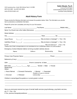
1215 Louisiana Ave., Suite 100, Winter Park, FL 32789 www.drrobinmeade.com
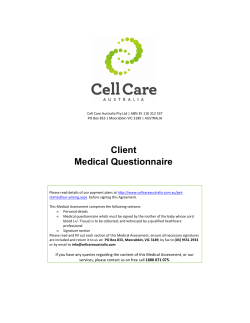
Client Medical Questionnaire
CANDIDA&QUESTIONNAIRE& Section(I(History( ( ( Point(Score______(
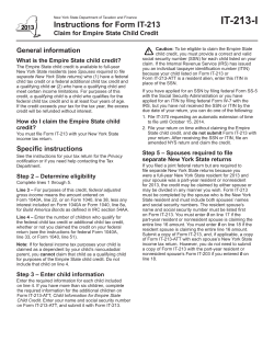
IT-213-I Instructions for Form IT-213 General information Claim for Empire State Child Credit
Social Security Administration Review Of Your Eligibility For Extra Help
Living Together Community Legal Information Association of Prince Edward Island, Inc. Introduction
606 24 Ave S, Suite 500 Minneapolis, MN 55454
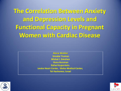
The Correlation Between Anxiety and Depression Levels and Functional Capacity in Pregnant
L ANGUAGES
© Copyright 2026
About abcdocz
DMCA / GDPR
Report