1. science
2. mathematics
3. statistics

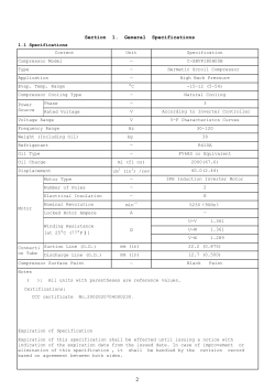
Proceedings of ICFD11:
Proceedings of ICFD11:
Eleventh International
Conference
of
Eleventh International
Conference
of Fluid Dynamics
Fluid
Dynamics
December
19-21, 2013, Alexandria, Egypt
December 19-21, 2013, Alexandria, Egypt
ICFD11-EG-4XXX
ICFD11-EG-4103
Design and Optimization of a Multi-Stage Axial-Flow Compressor
Prof. Dr. Atef M. Alm-Eldien
Mech. Power Eng. Dept.
Faculty of Eng.
Vice-president
for Students Affairs
Port-Said University, Egypt
[email protected]
Prof. Dr. Ahmed F. Abdel Gawad
Mech. Power Eng. Dept., Faculty of Eng.,
Zagazig Univ., Egypt
Currently:
Mech. Eng. Dept.
College of Eng. & Islamic Architecture
Umm Al-Qura Univ., Saudi Arabia
Fellow IEF, Assoc. Fellow AIAA
Member ASME, ACS, SIAM, AAAS
Prof. Dr. Gamal
Hafaz
Mech. Power Eng. Dept.
Faculty of Eng.
Port-Said University
Egypt
Eng. Mohamed G. Abd El Kreim
M.Sc. in Mech. Power Eng.
Steam Turbine Maintenance Engineer
Abou Sultan Power Plant
East Delta Electricity Production Company
Egyptian Electricity Holding Company
Egypt
[email protected]
[email protected]
I. INTRODUCTION
I.1 Previous Investigations
ABSTRACT
The objective of this paper is to define a methodology
for the design and analysis of multistage axial-flow
compressors. A numerical methodology is adopted for
optimizing the efficiency at the design point of a fifteenstage axial-flow compressor with inlet guide vanes (IGV).
The calculations are carried out along the mean streamline
using the principals of thermodynamics and aerodynamics.
A computer program was developed that simulates the
compressor model. By specifying the geometry
specifications (tip clearance, aspect ratio, thickness-chord
ratio, blockage factor, etc.) and design parameters (mass
flow, rotational speed, number of stages, pressure ratio,
etc.), an accurate numerical model can be generated. This
modeling technique is much simpler than the usual
computational methods that need much more
modeling/programming effort and computer run-time.
Starting from a newly-designed axial-flow compressor, an
optimized version is obtained with improved design-point
efficiency. So, once we get the optimized geometry of the
compressor, the original geometry is altered to maximize
the efficiency at the design-point. Concerning the optimized
version, analytical relation between the isentropic
efficiency of the compressor and the flow coefficient, the
work coefficient, the flow angles and the degree of reaction
are obtained.
KEYWORDS
Axial-flow
optimization.
compressor,
Efficiency,
There is a large volume of literature on compressor
design and its design parameters. However, the design
method is different from one research to another. The
intention of this review is to show the reader the related
work and to orient the reader where the current work stands
in relation to the literature.
Barbosa [1] used a streamline curvature for the flow
calculation along a multi-stage axial compressor of known
geometry. In his work, many streamlines are adopted from
hub to tip of the blades and divided in sections applied at
the inlet and outlet of each row. Hence, all flow properties
can be determined at each point of the intersection among
the sections of the cascade and the streamlines forming
control surfaces. Teinke [13] used a mean-line stage
stacking method for axial-compressor prediction. In his
method, the calculations are based on the mean streamline
of the axial-compressor channel. The flow properties such
as temperature, pressure, velocity and the dimensions of the
equipments including the balding angles are determined at
half blade. He stated that his method, when simulated in
computer, presented fast numeric convergence and
sufficient accurate results for a first analysis of the
compressors performance. Casey [3] presented a
computational program to calculate the efficiency of a
single-stage axial compressor to analyze the onedimensional condition with a pressure ratio of 1.2. The
author described the importance of analyzing the incidence,
deviation, profile losses, secondary losses and boundarylayer limits from hub tip related with the tip clearance in
order to predict the axial-compressor performance. The
deviation angle was obtained through Carter's rule [2]. He
used Lieblein's model [10] to calculate the profile losses.
The effect of the relative Reynolds number corrections to
the friction losses was calculated by Koch's model [8] and
Performance
1
the Mach number correction was done by Jansen, and
Moffatt procedure [7]. Seyb [12] presented a program for
the design and prediction of an eight-stage, constant outerdiameter, axial compressor.
As can be seen from the above literature survey, there is
a real need for a better direct method for the design and
optimization of the multi-stage axial compressor. The
method should consider all the parameters that affect the
compressor performance and be reliable for all the
compressor stages.
Therefore, a new method is introduced in this paper to
achieve these objectives. The method is fully explained in
the following sections.
I.2 Present Study
This paper is divided in two main parts. The first part
concerns the design of the axial-flow compressor. A
computer program is developed for this purpose by the
commercial software "Visual Basic". Figure 1 shows a
layout of the program window. The input data are typed in
the left portion of the window. The program uses
"Engineering Equation Solver (EES)" [15] to obtain air
properties at different steps of calculation. The program is
developed using the thermodynamics and aerodynamics
correlations. The results of the program represent an
important preliminary design-step that can be further tuned
using the Computational Fluid Dynamics (CFD)
simulations. When the program finishes calculation, three
graphs are obtained. The upper graph illustrates the
variation of geometry over the length of the compressor.
The lower-left graph shows the velocity diagrams
(triangles) in a particular stage. The third graph (lowerright) is to check the surge situation. The user can choose
the stage that he wishes to check. The results of the
program were validated using the data of reference [6]. The
validation covers the data of a fifteen-stage axial-flow
compressor. Generally, good agreements were achieved for
the geometry and dimensions as well as gas parameters.
Fig. 2 Layout of the optimizing program window after
finishing calculation.
The second part of this paper is devoted to the
optimization of design-point efficiency. A second program
was developed to maximize the efficiency at design-point
according to some constraints. So, the geometry of the
compressor that is obtained by the first program is fed to
the second program, where an analytical relation between
the efficiency and different design parameters is obtained.
II. ANALYSIS
II.1 Axial-Flow Compressor Design
The design process starts with the calculation of the
areas at the channel inlet and exit to accommodate the
desired mass flow-rate and pressure ratio. Then, the
calculation of both the total pressure and total temperature
at the inlet and outlet of each stage is carried out.
Consequently, velocity triangles, blade angles and losses
are calculated to end up with an estimation of the design
performance. The calculation process is divided into
separate modules. Figure 3 illustrates the overall structure
of the calculation process for the whole compressor.
Fig. 1 Layout of the program window after finishing
calculation.
Fig.3 Overall structure of the calculation process
for the whole compressor.
2
Cx
• Assumptions
1.
Two-dimensional flow.
2.
Identical balding (α1 = α3) at the mean radius.
3.
Constant mean radius.
As the fluid is taking its way towards the end of the
compressor, boundary layer starts to grow on the
compressor housing. This results in narrowing the path of
the fluid flow. This phenomenon is accounted for by the
introduction of a suitable blockage factor.
To achieve a prescribed duty case, the calculation
process encompasses the following steps:
1.
Selection of the duty coefficients (Ø) and number of
stages to achieve the specified compressor design flowrate and pressure ratio.
2.
Calculation of the air angles for each stage at the mean
radius.
3.
Determination of the variation of the air angles from
root to tip.
4.
Blade pitch chord ratio may then be selected to satisfy
aerodynamic loading parameters such as lift coefficient
and diffusion factor.
Fig.5 Assembled velocity triangles for a stage.
• Dimensionless velocity triangles
Considering the velocity triangle of a single stage,
Fig. 3, we can see that the overall shape of the velocity
triangles is governed by the three velocities Cx, ΔCθ and U.
We can show that Cx, and ΔCθ are related to the flow
coefficient φ and work coefficient ψ as follows:
Fig.4 Meridional view of a multi-stage compressor.
φ = c x from which we get
The meridional view of a multi-stage compressor that is
shown in Fig. 4 illustrates the main features of blading and
annulus:
1. An inlet guide vane blade row to provide pre-whirl
into the first stage.
2.
U
cx = φ U
Δ
ψ = h2o
U
From
Euler
pump,
Δ h o = U( c θ 2 − c θ1 ) = UΔ cθ
A set of repeating stages, each comprising a rotor
followed by a stator.
From which we get Δ c θ = ψU
3
(1)
Eq. 3,
we
get
(2)
To make the velocity triangles dimensionless, we divide
all velocities by the blade speed U. The outcome of this is
shown in Fig. 4 from which important results is obtained.
α =α
1
⎛1⎛
1 ⎞ ⎞ Inflow
= arctan ⎜⎜ ⎜ 1 − R − ψ ⎟ ⎟⎟
2 ⎠⎠
⎝φ ⎝
3
⎛1⎛
1 ⎞ ⎞ Outflow angle
= arctan ⎜⎜ ⎜ 1 − R + ψ ⎟ ⎟⎟
2 ⎠⎠
⎝φ ⎝
⎛1⎛
1 ⎞ ⎞ Relative inflow angle
β 1 = arctan ⎜⎜ ⎜ R + ψ ⎟ ⎟⎟
2 ⎠⎠
⎝φ ⎝
α
⎛1⎛
1 ⎞⎞
⎜ R − ψ ⎟ ⎟⎟
φ
2 ⎠⎠
⎝ ⎝
w1 = φ 2 + ⎛ R + ψ ⎞
⎜
⎟
U
2 ⎠
⎝
w2 =
U
2
Relative outflow angle
2
Rotor relative outflow velocity
⎛ ψ⎞
φ 2 + ⎜ R− ⎟
−
h
1
=
−
h
2
2
⎛
⎞ ⎛
⎞
= ⎜ h 02 − c 2 ⎟ − ⎜ h 01 − c 1 ⎟ =
⎜
2 ⎟ ⎜
2 ⎟
⎝
⎠ ⎝
⎠
h
⎜
⎝
h
03
−
2 ⎟
⎠
−
⎜
⎝
h
01
−
2 ⎟
⎠
=
h
03
01
= Δ
h
h
2
h
1
02
−
h
(
) (
)
c θ 2 − c θ 1 = (c θ 2 − c θ 1 )(c θ 2 + c θ 1 )
2
2
Introducing Eq. 6 into Eq. 5, we have
Δ h0
(c θ 2 + c θ 1 )
h 2 − h1 = Δ h 0 −
2U
So, the reaction R becomes
1
(c + c )
R = 1−
2U θ 2 θ 1
From which
cθ 2 + cθ 1 = 2U (1 − R )
Thus, we have
cθ 1 = 1 − R − 1 ψ
U
2
cθ 2 = 1 − R + 1 ψ
U
2
0
(5)
01
L
Rotor entry and stage exit
2
Stator inflow velocity
(21)
1
l
2
m
D
m
But we have
tan β =
1
1⎛
1 ⎞,
⎜R + ψ ⎟
2 ⎠
1⎛
1 ⎞
tanβ = ⎜ R − ψ ⎟
2 φ
2 ⎠
⎝
φ⎝
(23)
Hence,
(6)
tan
β
m
=
( β
1
tan
2
1
+ tan
R
β )= φ
(24)
2
Substituting these into Eq. 22, we have the alternative form
for CL involving the duty coefficients ( φ , ψ):
(7)
(8)
C
L
⎛t
= 2⎜
⎝l
⎡
⎤
2ψ
R
⎞⎢
⎥
− ( )C D
⎟⎢
φ
⎠ ⎢ 4 2 + 1 ⎥⎥
φ ⎦
⎣
(25)
(9)
Considering the drag coefficient, defined by
(10)
CD = 1
2
(11)
wθ 1 = 1 − cθ 1 = R + 1 ψ
(26)
⎛t⎞
= ζ ∞ ⎜ ⎟ cos β ∞
2
⎝l⎠
ρ w∞ l
D
Where, the cascade loss coefficient is based on the vector
mean velocity w∞
(12)
2
wθ 2 = 1 − cθ 2 = R − 1 ψ
(13)
U
U
2
We note that the dimensionless velocity triangles and
hence the blade shapes required to achieve them are totally
determined by the stage duty coefficients φ ,ψ and R.
It follows that all angles and velocities may be expressed
as functions of φ andψ as follows:
U
2
The dimensionless parameters that indicate profile
aerodynamic quality are the lift and drag coefficients CL
and CD. It is important therefore to express CL and CD in
terms of the duty coefficients which have a total control
over the shape of the velocity triangles. Lift coefficient for
a cascade can be expressed in terms of the relative inflow
and outflow angles β1 and β2, the vector mean of them β∞
and the pitch to chord ratio, t/l as follows:
t
(22)
C = 2 (tan β − tan β )cos β − C tan β
But since there is no work or heat input through the
stator, h02 = h03 and thus h02 - h01 = h03 - h01 = Δh0. Also,
since the axial velocity is assumed to be constant, we have
2
2
2
2
2
2
c 2 − c1 = c x + c θ 2 − c x + c θ 1 =
(19)
• Lift and drag coefficients in terms of duty coefficients
Then, the numerator is written as
−
(17)
(20)
c 2 = φ 2 + ⎛ 1− R + ψ ⎞
⎜
⎟
U
2 ⎠
⎝
Since the stages are repeating for which entry and
leaving velocities are identical, C3 = C1, the denominator of
Eq. 3 may be simplified to
2
2
⎛
(4)
c 3 ⎞⎟ ⎛⎜
c 1 ⎞⎟
⎜
3
(16)
2⎠
⎝
velocities
Swirl velocities Wθ2 and Cθ1 can be related to φ ,ψ and
R as follows
−
(3)
R = h 2 h1
−
h 3 h1
(15)
Rotor relative inflow velocity (18)
c 1 = c 3 = φ 2 + ⎛ 1− R − ψ ⎞
⎜
⎟
U
U
2 ⎠
⎝
Fig.6 Dimensionless velocity triangles for a stage.
(14)
2
β 2 = arctan ⎜⎜
h
angle
U
ζ∞=
(Δ p0)loss
Since,
4
(27)
1
2
ρW ∞
2
ζR=
Δ
poR &
1
ρ W 12
2
ζs=
Δ p os
1
ρ C 22
2
(28)
Where, ζR,ζs are the rotor and stator loss coefficients
expressed in terms of the exit velocities C2 and w3 relative
to the blade rows.
Hence, we get
2
2
Δ poR
ζR=
1
ρ W 12
2
(29)
⎛ cos β 1 ⎞
⎛ w∞ ⎞
⎟⎟ = ζ ∞ ⎜⎜ cos β ⎟⎟
w
⎝ 1⎠
∞⎠
⎝
= ζ ∞ ⎜⎜
So that CD becomes
(
2
2
3
cos β ∞
⎛ t ⎞ 2φ 4 φ + (1 + φ )
= ζ 1⎜ ⎟
3
⎝ ⎠ cos 2 β 1
⎝l⎠
4φ 2 +1 2
⎛ ⎞
C D = ζ 1⎜ l ⎟
t
(
)
)
(30)
From the definition of diffusion factor (DF), Lieblein et al.
[10], we have
DF = 1 −
cos
cos
β1
β2
+
β1⎛t ⎞
cos
(
⎜ ⎟ tan
⎝l⎠
2
β 1 − tan β 2 )
(31)
The rotor and stator blade rows will have different profile
geometry. In order to select suitable values of pitch/chord
ratio t/l to control aerodynamic loading, we have for the
rotor
2
2
(32)
4φ + (1−ψ )
t
ψ
DF
R
= 1−
4φ +
2
(1−ψ )
2
⎛ ⎞
+⎜ ⎟
⎝l⎠ 4 2+
φ
(1−ψ )
2
And for the stator, we have
DF
= 1−
S
⎞
⎜ ⎟ (tan α − tan α )
cos α
2
⎝l ⎠
φ + (1− R −ψ / 2 ) + 1 ⎛ t ⎞
ψ
⎜ ⎟
2
+
φ (1− R −ψ / 2 ) ⎝ l ⎠ φ + (1− R +ψ / 2 )
= 1−
cos α 2
+
cos α 2 ⎛ t
3
2
Fig.7 Flowchart showing the iterative process for axial
velocity.
(33)
3
s
2
2
2
2
2
• Calculation of static properties
2
s
Before the calculation begins, the inlet geometry must
be determined. To be able to find the inlet geometry, the
inlet flow velocity Cm must be known. Since this velocity is
unknown, an iterative process is made to find Cm. With the
help of mass continuity, a new flow velocity is calculated.
This value is then used to start over the calculation until
convergence is accomplished. The first step is to get the
thermodynamic properties at the inlet of the compressor.
The ambient pressure and temperature are known and from
them Cp and γ are determined. With these properties are
known, the iteration process can begin, Fig. 7.
Fig.8 Compressor stage (T-S) diagram.
5
• Calculation of the equivalent diffusion ratio (Deq*)
• Calculation of static pressure and temperature at
rotor inlet (P1, T1)
1.
2.
3.
4.
cos(β 2) ⎡
From EES, find h01, S01, K01 and Cp01 using (P01, T01).
Find h1 = h01 - C12/2.
From EES, find ρ1, Cp1, k1 and μ1 using (h1, S1 = S01).
Find T1 = T01 - (C12/2 × Cp1).
Deq* = cos( ) ⎢1.12 + 0.61
β1 ⎢
2
cos (β1)
⎣
⎛ k ⎞
⎜ 1 ⎟
σ
⎤
(tan(β 2) − tan(β1))⎥⎥
(35)
⎦
• Calculation of the compressor losses
⎛
⎞⎜ k −1 ⎟
5. Find p = p ⎜ T 1 ⎟⎝ 1 ⎠
1
01 ⎜
⎟
⎝ T 01 ⎠
• Calculation of static pressure and temperature at
rotor outlet stator inlet (P2, T2)
• Profile loss model
The profile loss model used is a modified version of the
two-dimensional low speed correlation of Lieblein
et al. [10], Fig. 9.
1. Find compressor exit temperature
⎛ 1 ⎞⎛ k −1 ⎞
⎜
⎟⎜ 01 ⎟
⎜ η ⎟⎜ k
⎟
p
⎝
⎠⎝ 01 ⎠
(π )
Te
01
2. Find stage temperature rise ΔT=(Te-T01)/n_stg
3. Find T03 = T01 + ΔT
=T
⎛ k1 ⎞
⎜
⎟
4.
5.
6.
7.
8.
9.
⎜ k −1 ⎟
Find p = p ⎡1+ η p Δ T ⎤ ⎝ 1 ⎠
⎢
⎥
03
01
T 01 ⎦⎥
⎣⎢
P02 = P03, T02 = T03
From EES find h02, S02 using P02, T02
Find h2 = h02- C22/2
From EES find ρ2, Cp2, k2, μ2 using h2, S2 = S02
Find T2 = T02 - (C22 / 2 × Cp2)
⎛ k
⎞
2 ⎟
⎜
⎜
−1 ⎟
10. Find p = p ⎛⎜ T 2 ⎞⎟ ⎝ k 2 ⎠
2
02 ⎜
⎟
⎝ T 02 ⎠
• Calculation of static pressure and temperature at
stator outlet (P3, T3)
1. From EES find h03, S03 using P03, T03
2. Find h3 = h03 - C32/2
3. From EES find ρ3, Cp3, k3, μ3 using h3, S3 = S03
4. Find T3 = T03 - (C32/2 × Cp3)
5.
⎛
Find p = p ⎜ T
3
03
Fig. 9 Profile loss parameter with variation of Mach
number [10].
The profile loss parameter is expressed as
ζ
⎞
⎛ k
3 ⎟
⎜
⎜ k −1 ⎟
⎞
3 ⎟⎝ 3 ⎠
f ( x) = a 0 + a1 x + .... + a n −1 x n −1 + a n x n
The starting rotor inlet-conditions will have the same
velocity and radius outlet of the previous stage and the
stagnation properties is taken from the previous stage.
• The polynomial coefficients are listed below
rm,1 = rm,3(i-1), Cm,1 = C m,3(i-1), α1 = α3(i-1)
P01 = P03 (i-1), T01 = T03 (i-1), h01 = h03 (i-1), S01 = S03 (i-1)
• Calculation of the pitch-chord ratio (s/c)
The calculation of the pitch-chord ratio is based on the
diffusion ratio. The input parameters consist of the relative
inlet and outlet flow angles, the different axial velocities
and radiuses and also the diffusion factor
M1
a0
a1
a2
a3
a4
0.3
-8.26097e-02
2.62982e-01
-2.66675e-01
1.14774e-01
-1.61839e-02
0.7
-1.30107e-01
3.68490e-01
-3.56939e-01
1.48500e-01
-2.08264e-02
1.0
-1.36535e-01
3.78126e-01
-3.66336e-01
1.52219e-01
-2.13465e-02
• End-wall loss
A correlation is used to determine the end-wall losses
based on a numerous sets of compressor data where the
parameters, tip clearance, aspect ratio, and mean-line
loading where systematically varied. These parameters can
be correlated as in Fig. 10, [4].
(β 1 , β 2 , c m1 , c m2 , r m1 , r m2 , DF )
⎞
w 2 ⎞⎟ ⎛⎜
r1 + r 2
⎟
⎟ w1 ⎜
w1 ⎠ ⎝ r 2 wθ 2 − r 1 wθ 1 ⎟⎠
(36)
v2
A fourth-order polynomial fitting method has been used to
interpret the graph that has the form
⎜T ⎟
⎝ 03 ⎠
The above calculation process is repeated for each stage
noting that:
S ⎛⎜
= DF − 1 +
C ⎜⎝
2
0.5 v12 cs(α 2) = f ( M 1 , D eq )
p
(34)
6
dynamic head, the minimum dynamic head and the
dynamic head at zero axial velocity as given by the
following equation, Fig. 11.
F
ef
=
2
C + 2 .5 C
2
min
+ 0 .5 U 2
4C 2
(40)
2
C min =
2
sin (α + β ), if (α + β ) ≤ 90 and β ≥ 0
2
C
2
C min = 1, if (α + β ) > 90
2
C
2
2
C min = U 2 if β < 0
2
2
C
C
Fig. 10 End-wall loss parameter with variation of tip
clearance.
The end-wall loss parameter is expressed as
h 2
ζ e v12 =
c v2
⎛ε
⎞
f ⎜ , DF ⎟
⎝C
⎠
(37)
A fourth-order polynomial fitting method has been used to
interpret the graph it has the form
f ( x) = a 0 + a1 x + .... + a n −1 x n −1 + a n x n
• The polynomial coefficients are listed below
Tip
Clearance
a0
a1
0.0
3.23881e00
-3.66895e01
1.60855e02 -3.14825e02 2.32625e02
0.02
2.86933e00
-3.18679e01
1.36001e02 -2.58533e02 1.85224e02
0.04
-2.00381e-01
1.04984e00
3.12191e00
0.07
8.18792e-01
-8.62635e00
3.57996e01 -6.61454e01 4.61697e01
0.1
2.38135e-01
-2.36201e00
1.01622e01 -1.92343e01 11.36794e01
•
a2
a3
-2.0345e01
a4
Figure.11 Diagram giving definition of Fef.
Figure 12 shows a correlation of stalling pressure-rise
coefficient (CpD) and of diffusion-length to exit passagewidth (L / g2).
2.48570e01
L
g2
=
σ
( )
⎛θ ⎞
cos β b 2 cos⎜ ⎟
⎝2⎠
Calculation of the stall/surge
A relationship created by Koch [8] is used to determine
how close a stage to stall/surge. By calculating the static
pressure rise coefficient, Cp, based on pitch-line dynamic
head, and comparing it to the maximum static pressure rise,
Cp,max, a good indication of how close a stage is toward stall
is given. The static pressure-rise coefficient and the
maximum pressure-rise coefficient are as follows:
cp
⎡
⎢⎛
c p T 1 ⎢⎜⎜
⎢⎝
⎢⎣
=
k −1
k
⎤
⎥
− 1⎥ −
⎥
⎥⎦
2
2
W1 −C2
2
p3 ⎞
⎟
p 1 ⎟⎠
(
(U 22 − U 12 )
2
)
⎛ Cp ⎞ ⎛ Cp ⎞ ⎛ Cp ⎞
⎟
Cp,max= CpDFef ⎜⎜ ⎟⎟ ⎜⎜ ⎟⎟ ⎜⎜
⎟
⎝ CpD⎠Re⎝ CpD⎠ε ⎝ CpD⎠Δz
(38)
(39)
Fig.12 Correlation of stalling pressure-rise
coefficient (CpD).
Where, Fef is the effective dynamic-pressure coefficient that
is represented by a weighted-average of the free-stream
7
(41)
A fifth-order polynomial fitting method has been used to
interpret the graph that has the form
f ( x) = a 0 + a1 x + .... + a n −1 x n −1 + a n x n
• The polynomial coefficients are listed below
a0
a1
a2
a3
a4
a5
7.6431e-02 4.916e-01 -2.5166e-01 9.1688e-02 -1.9627e-02 1.7779e-03
Figure 13 shows the effect of tip clearance on stalling
pressure-rise coefficient (CpD).
g=
( ( )
( ))
π r m cos β b1 + cos β b2
•
Fig. 14 Effect of axial-spacing on stalling pressure-rise
coefficient (CpD).
(42)
Z
Where, Z denotes the number of blades in one row.
Figure 15 shows the effect of Reynolds number on stalling
pressure-rise coefficient (CpD).
The polynomial coefficients are listed below
a0
a1
a2
a3
a4
a5
1.1191e00 -6.1567e-01 9.6073e-01 -2.2107e-01 -7.4519e-01 5.1421e-01
Fig. 15 Effect of Reynolds number on stalling pressurerise coefficient (CpD).
A function of the type f (x ) = a x b + C is used for
the interpretation of Fig. 15. The coefficients of the
function are:
Fig. 13 Effect of tip clearance on stalling pressure-rise
coefficient (CpD).
Figure 14 shows the effect of axial-spacing on stalling
pressure-rise coefficient (CpD).
• The polynomial coefficients are listed below
a0
a1
a2
a3
1.21683e00 -1.00986e01 2.424416e02 -3.38124e03
a4
a5
b
c
-101.8
-0.6767
1.041
• Calculation of blade angles
Various angles at the inlet and outlet of the blade are
shown in Fig. 16.
2.20418e04 -5.35103e04
The axial-spacing between rows is given by:
ΔZ = 0.2 C
a
(43)
8
Ksh
Blade Type
0.7
DCA
1.0
65-SERIES
1.1
C- SERIES
2
⎛t⎞
⎛t⎞
⎛t⎞
k it = −0.0214 + 19.17⎜ c ⎟ − 122.3 ⎜ ⎟ + 312.5 ⎜ ⎟
⎝ ⎠
⎝c⎠
⎝c⎠
3
(45)
i 010 = (0.0325 − 0.0674σ ) + (− 0.002364 + 0.0913σ )α 1
+ (1.64e − 05 − 2.38e − 04σ )α 12
n = (− 0.063 − 0.02274σ ) + (− 0.0035 + 0.0029σ )α 1
− (3.79e − 05 + 1.11e − 05σ )α 12
Fig. 16 Various angles at the inlet and outlet
of the blade.
• Calculation of the deviation angle
It is the difference between outlet blade-angle and outlet
flow-angle. It arises from a combination of two effects.
First, the flow is decelerating on the suction surface and
accelerating on the pressure surface as it approaches the
trailing edge. As a result of that, the streamlines are
diverging on the suction surface and converging on the
pressure surface so that the mean flow-angle is less than the
blade angle. Second, the rapid boundary-layer growth on
the suction surface towards the trailing edge pushes the
streamlines away from the surface. The correlation for the
deviation angle is given by:
• The blade angles are
α'1 = α1 – γ
α'2 = α2 – γ
Where, α1 is the blade inlet angle and α'1 is the flow
inlet angle, α'2 is the blade outlet angle, α2 is the flow outlet
angle and γ is the stagger angle.
i = α1- α'1
δ= α'2- α2
θ
δ = mc + x
σ
Where, i is the incidence angle which is the difference
between the flow inlet angle and the blade inlet angle, δ is
the deviation angle which is the difference between the
flow outlet angle and the blade outlet angle.
(46)
δ (i = i ref ) = k sh k δ t δ
010
+ mθ
⎛
⎛t ⎞
k δ t = 0 . 0142 + 6 . 172 ⎜ c ⎟ + 36 . 61 ⎜
⎝ ⎠
⎝
The fluid deflection and the camber angles are defined by
(47)
(i 010 θ )
t ⎞
⎟
c⎠
2
(48)
δ 010 = (0.0443 + 0.1057 σ ) + (0.0209 − 0.0186 σ )α 12
(− 0.0004 + 0.00076 σ )α 13
θ = α'1 + α'2
ε = α1+ α2 = (i + α'1) + (α'1 – δ) = ( α'1 + α'2) + (i - δ)
m = m
b
=(θ + i -δ)
'
(49)
α
2
1
+ 2 . 538 e − 03
• Calculation of the incidence angle
− 1 . 3 e − 06
α
Incidence is the difference between the inlet blade-angle
and the inlet flow-angle. As the fluid flows towards the
leading edge, it experiences "induced incidence". There is a
pressure and a suction surface at a given blade. This
difference of pressure changes the ingoing flow angle as it
approaches the leading edge. The correlation for the
incidence angle is given by:
m' is different based on the blade type, DCA, C-series or a
65-series
i ref = k sh k it i 010 + n θ (i 010 , θ )
1
+ 4 . 221 e − 05
α
b = 0 . 9655
3
1
For a 65-series
m = 0.17 − 3.33e − 04(1− 0.1α1)α1
'
(49.a)
For DCA, C-series
(44)
'
2
m = 0 . 249 + 7 . 4 e − 04 α 1 − 1 . 32 e − 05 α 1 (49.b)
Ksh and kit are corrections factors for blade shape and
thickness, respectively, Ksh differs whether the blade is a
DCA,65-series or a C series [4].
3 . 16 e − 07
9
α 13
By applying Buckingham's π-theorem and applying
dimensional analysis, Eq. 50 may be simplified to the
following dimensional form:
II.2 Design Optimization of Axial-Flow Compressor
Once we get the geometry supplied by the program of
the axial-flow compressor design-point efficiency, its
geometry is altered to maximize efficiency at the designpoint. The structure of the optimizing program is shown in
Fig. 17.
η tt =
⎛
f ⎜⎜ φ ,ψ , R , w1 , c 2 , M 1 , M 2 , R em , ζ
U U
⎝
R
⎞
, ζ s ⎟⎟
⎠
(51)
Where M1 and M2 are the rotor and stator exit mach
numbers that are defined as:
M1=
W1
a1
M2 =
C2
a2
(52)
Rem is the stage Reynolds number based on mean radius
U rm
(53)
Rem =
ζ
υ
,
are the rotor and stator loss coefficients expressed
R ζs
in terms of the exit velocities C2 and w3 relative to the blade
rows.
Δp
ζ R = 1 oR
ρ W 12
2
ζs=
Δ pos
1
ρ C 22
2
(54)
φ , ψ are the flow and work coefficients defined as
φ = Cx
U
Ψ= Δ ho
(55)
U
• Independent design variables
Fig.17 Structure of the optimizing program of the axialflow compressor.
The designer is free to select the design duty
coefficients ( φ , ψ). As these duty coefficients have a
profound effect upon the stage efficiency ηtt even with
optimum aerodynamic design. φ and ψ control the shape of
the velocity triangles and thus the flow environment within
which the blades operate. Also, the degree of reaction (R)
has a direct control over velocity triangle shape and hence
efficiency.
By applying dimensional analysis for a single stage and
making the following assumptions:
Constant axial velocity Cx.
Constant mean radius rm = 1/2(rh + rt).
Identical velocity vectors C1 and C3 at entry to and exit
from the stage at the mean radius rm.
1.
2.
3.
The efficiency ηtt of this stage is dependent upon the
following variables, [9]:
⎛ Δ h o , h1, h 2 , h 3 ω , r m , c x , w 3 ,⎞
(50)
⎟
η = f⎜
tt
⎜c2,μ,ρ,a
⎝
2
,a3,Δ
• Dependent design variables affecting (ηtt)
Experimental cascade tests show that the loss
coefficients ζ R , ζ s are themselves dependent upon blade
p or , Δ p os ⎟⎠
• Thermodynamic variables. The stage stagnation enthalpyrise Δho determines the specific work input and signifies
stage loading. The specific enthalpies h1, h2 and h3 typify
the progression in energy transfer through the stage. All
four are independent variables.
• Speed and size. Both are independent variables.
• Velocity triangles. Four velocities are required to
determine the shape of the velocity triangles these are the
blade speed U = rm ω, Cx as an independent variables, C2,
W1 are dependent variables.
• Properties of working substances. The dynamic viscosity
μ, density ρ and speeds of sound a1, a2 depend on the
physical and thermodynamic properties of the gas.
• Losses. The stator and rotor losses from all sources
(profile drag, tip clearance loss, etc.) are lumped into
stagnation pressure losses Δpos and Δpor.
row Reynolds number and inlet Mach number. We would
also expect that loss levels to be directly influenced by the
velocity triangle environment within which the blades have
to operate and hence to depend upon φ , ψ and R. We can
express this through [9],
ζ
R
ζ
s
= f 1 (φ ,ψ , R , Re R , M 1)
=
f
2
(φ ,ψ , R , Re s , M 2 )
(56)
Where, the blade row Reynolds numbers ReR and Res
are based on rotor and stator blade chords lR and ls.
W 1l R
Re R = υ
C2 ls
Res = υ
10
(57)
Equation 51now is simplified into
η tt = f (φ ,ψ , R , , ζ R , ζ s )
η tt
=1−
(58)
1 ⎛ 2 1
⎜φ +
2ψ ⎝
4
1. The stage duty coefficients ( φ , ψ).
2. The blade-row loss-coefficients
The initial selection of the stage duty coefficients ( φ ,
ψ) is crucial. Thus, we could rewrite Eq. 64in the form
Equation 58 can be converted into a more useful
analytical form. By assuming for the moment a fixed
reaction value R = 0.5. From h0 – S diagram, Fig. 18, by
defining the stagnation enthalpy loss due to irreversibility
into
η tt = 1 − f c (φ ,ψ )(ζ R + ζ s )
(59)
(Δp)loss, Eq. 63 Substituting the value of W1/U and C2/U into
Eq. 63, we have
(Δ p 0 )loss
Hence, the total to total efficiency.
ρU
(Δ h0)loss (Δ p0)loss 1 ⎛⎜ (Δ p0)loss ⎞⎟ (61)
h −h
= 1−
= 1−
η tt = 03s 01 = 1 −
ρ Δh0
ψ ⎜ ρU2 ⎟
Δ h0
h03 − h01
⎝
⎠
1
2
ρU2
2
2
ζ
R
2
=
1
2
2
ζ
R
2
1
⎛ w1 ⎞
⎛C ⎞
⎜
⎟ + ζ s⎜ 2 ⎟ =
2
⎝U ⎠
⎝ U ⎠
2
⎡
⎢φ 2 + ⎛ R + ψ ⎞ + 1
⎜
⎟
⎢
2
2 ⎠
⎝
⎣⎢
ζ
s
(67)
2⎤⎤
⎡
⎢φ 2 + ⎛⎜ 1 − R + ψ ⎞⎟ ⎥ ⎥
⎢
2 ⎠ ⎥⎦ ⎥⎥
⎝
⎣
⎦
The total to total efficiency then follows by substituting into
Eq. 61 to get
(62)
Substitution of Eq. 54 in Eq. 61results in the dimensionless
loss.
2
(66)
⎠
The loss coefficients for the rotor ζ R and stator
ζ s have been defined by Eq. 54 and the total stage loss
From the conventional definition of ηtt
= stagnation enthalpy rise for an ideal stage/stagnation
enthalpy rise for the actual stage
⎛ w1 ⎞ 1 ⎛ C2 ⎞ ⎛⎜ ζ R + ζ s ⎞⎟⎛ 2 1
2⎞
+
⎟ + ζ s⎜ ⎟ = ⎜
⎟⎜⎝φ 4 (1+ψ ) ⎟⎠
2
2
U
U
⎝ ⎠
⎝ ⎠ ⎝
⎠
)2 ⎞⎟
• Stage losses and efficiency
(60)
ζ R⎜
(
minimized by the careful blade profile design unless the
duty coefficients ( φ , ψ) and velocity triangles are badly
chosen in the first place, resulting in an excessive value of
fc.
The stage stagnation enthalpy rise is given by
(Δ p0)loss = 1
1 ⎛ 2 1
⎜φ + 1+ψ
2ψ ⎝
4
ζ R and ζ s are normally used to represent cascade loss
coefficients. We need to pin into all other frictional losses
such as tip leakage and secondary losses related to the rotor
and stator. From the stage performance analysis, the
inherent aerodynamic loss character tics of the blades can
be summarized [9]. From Eq. 66 fc depends upon duty
coefficients ( φ , ψ) and thus the velocity triangle
environment into which the blades are immersed. fc is called
a "Weighting Coefficient" as it gives weight to the
aerodynamic loss coefficients ζ R and ζ s which can be
Fig. 18 T-S and h0-S diagrams for
an axial-compressor stage.
Since, (Δ p 0) = (Δ p 0 R ) + (Δ p 0 s )
loss
loss
loss
(65)
Where, the loss-weighting coefficient ( fc) is given by
f c (φ ,ψ ) =
Δ h0 = h03 − h01
ζ R and ζ s (i.e., blade-
row aerodynamic).
• Simple analytical formulation for the total to total
efficiency of a compressor stage
= h 03 − h 03 s
(64)
⎠
Equation 64 is equivalent to the parametric Eq. 58
derived from the dimensional analysis for a 50% reaction.
But it is in the much more useful explicit form of an
analytical relationship which shows how ηtt depends upon
the various dimensionless groups. From this, we can deduce
that the efficiency of a 50% axial-compressor stage is
dependent upon two main factors:
Thus, the efficiency of an axial-compressor stage
depends upon five dimensionless parameters which are
sufficient to account for all the 15 items listed in Eq. 50Of
these parameters, just three may be independently selected
by the designer, namely φ , ψ and R. The loss coefficients
themselves are also dependent upon the duty parameters φ ,
ψ and R but in addition are influenced by Reynolds number
and Mach number.
(Δ h 0 )loss
(1+ψ )2 ⎞⎟ (ζ R + ζ s )
η tt = 1 −
⎧
1 ⎪
⎨ζ
2ψ ⎪
⎩
2⎤
⎡
⎢φ 2 + ⎛⎜ R + ψ ⎞⎟ ⎥ + ζ
R⎢
2 ⎠ ⎥⎦
⎝
⎣
2⎤ ⎫
⎡
⎢φ 2 + ⎛⎜1− R + ψ ⎞⎟ ⎥ ⎪⎬
s⎢
2 ⎠ ⎥⎦ ⎪
⎝
⎣
⎭
(68)
Eq. 68 is consistent with Eq. 61 as a result of linking stage
duty ( φ , ψ) and reaction R to velocity triangles and thus to
stage aerodynamics and thermodynamics.
(63)
Introducing Eq. 63 into Eq. 61,we have
11
• Optimum reaction
III. Results and Discussions
III.1 Results of Design Program
For any prescribed ( φ , ψ) duty, we may estimate the
stage reaction R, which will produce maximum efficiency.
Eq. 68 can be written as.
(69)
η tt = 1 − L
At first we summarize the main steps in the design
procedure described in the analysis section. Having made
appropriate assumption about the axial velocity, it is
possible to calculate the annulus area at the inlet and outlet
of the compressor and calculate the air angles required for
each stage at the mean diameter. Then, by the use of vortex
theory, the air angles can be calculated at various radiuses
from root to tip. Throughout this work, there was a
limitation on blade stresses; rates of diffusion and Mach
number that were not exceeded. The results of the program
were validated using the data of Ref. [6]. The compressor
of the present study is a 15-stage axial compressor with
122 kg/s of air at ambient pressure of 1.013 bar and
temperature 288 K, pressure ratio 20 and polytropic
efficiency of 90%. Tables 1-5 show the present calculated
values and the relative differences in comparison to the data
of Ref. [6]. There is a good agreement as far as dimensions
are concerned and a reasonable agreement in the other
parameters. This may be attributed to some difference in
design assumptions. The biggest differences between the
present results and those of Ref. [6] are noticed in Table 5.
The difference in the inlet stator angle may reach about 7%.
Figures 19 and 20 show the rise of both the static
pressure and temperature through the compressor stages,
respectively. Figures 21-23 show the variation of air angles,
degree of reaction, rotor/stator exit Mach number from root
to tip for a selected stage (stage 10). In Fig. 21, the radial
variation of air angles of the rotor shows a change in fluid
deflection for a considerable twist along the blade height to
ensure that the blade angles are in agreement with the air
angles. In Fig. 22, the stator deflection is less in comparison
to the rotor deflection due to the nature of building-up
pressure in stator blades. In Fig. 23, the degree of reaction
increases from root to tip, which indicates a high mass
flow-rate per unit blade-height and thus plays an important
role in to raising the stage efficiency. Figures 24 and 25
show the rotor and stator end wall, profile and total losses.
Profile losses are contributed to boundary-layer separation
while end-wall losses are mainly due to secondary flow
effects and mixing for the rotor. The profile and end-wall
losses increase through the stages with the result of an
increase in total losses due to the increase in the work that
is required to accomplish fluid turning and raising the
pressure through different stages as well as the generation
of entropy. At the stator, the end-wall and profile losses
decrease, resulting in a decrease in total losses due to the
diffusing working nature of the stator blades.
Where, L is given by
L=
2
2
⎧ ⎡
⎡
ψ ⎞ ⎤⎥
ψ ⎞ ⎤⎥ ⎫⎪
1 ⎪ ⎢ 2 ⎛
2 ⎛
⎢
+
+
+
+
1
−
+
R
R
⎟ ζ s ⎢φ ⎜
⎟ ⎬
⎨ζ φ ⎜
2ψ ⎪ R ⎢
2 ⎠ ⎥⎦
2 ⎠ ⎥⎦ ⎪
⎝
⎝
⎣
⎩ ⎣
⎭
(70)
The minimum loss and therefore maximum efficiency
with respect to reaction R follows from
⎧ ∂L ⎫
(71)
=0
⎨ ⎬
⎩ ∂R ⎭φ ,ψ
Where φ and ψ are kept constant. If we assume that the
loss coefficients are weak function of R and may be
assumed constant also, then Eq. 71 yields to
ψ
R optimum = 2
(ζ s − ζ R )+ ζ s
ζ s +ζ R
(72)
One possible solution to this which is true for all values
of ψ is R = 0.5 and ζ s = ζ R . Although the stator and rotor
velocity triangles are identical for this condition of 50%
reaction, in reality there will be a difference in the two loss
coefficients. Even so the strong indication is that 50%
reaction will be close to optimum [9].
• Optimum ψ for a given φ and R
Alternatively, we may search for ψ value leading to
minimum loss for given φ and R values by writing
(73)
⎧ ∂L ⎫
⎨
⎬ =0
⎩ ∂ψ ⎭φ , R
Resulting in
ψ
optimum
= 2
φ
2
+
1
+ R (R − 1 )
2
Where, we have also assumed that ζ s and
(74)
ζ R are
independent of ψ. Two stages of special interest are the
50% reaction stages which we have already considered and
the 0% reaction or "impulse stages". For these two
reactions Eq. 74 becomes
2
(75)
= 4φ + 1
ψ
optimum
ψ optimum
=
2
4φ + 2
Table 1: Comparison of the present (AFCP) results and
the data of Ref. [6] for the compressor tip radius.
In practice the stator and rotor loss coefficients ζ s and
ζ R do vary with both φ and ψ and form experimental tests
the sensible design for ψ lies between the two values.
2
(76)
= 0 .185 4 φ + 1
ψ
Compressor Tip Radius (mm)
Present
Ref. [6] Diff. (%)
Stage Row
(AFCP)
1
0.524
0.528
0.773
1
2
0.513
0.513
0.024
3
0.505
0.507
0.416
1
0.505
0.507
0.416
2
2
0.496
0.5
0.799
3
0.490
0.494
0.749
3
1
0.490
0.494
0.749
opt ., exp
ψ max = 0 .32 + 0.2φ
12
4
5
6
7
8
9
10
11
12
13
14
15
2
3
1
2
3
1
2
3
1
2
3
1
2
3
1
2
3
1
2
3
1
2
3
1
2
3
1
2
3
1
2
3
1
2
3
1
2
3
0.483
0.479
0.479
0.473
0.470
0.470
0.471
0.468
0.468
0.464
0.462
0.462
0.458
0.457
0.457
0.453
0.452
0.452
0.449
0.449
0.449
0.446
0.445
0.445
0.443
0.443
0.443
0.441
0.440
0.440
0.438
0.438
0.438
0.437
0.436
0.436
0.435
0.435
0.489
0.484
0.484
0.480
0.476
0.476
0.474
0.470
0.470
0.467
0.464
0.464
0.462
0.460
0.460
0.457
0.455
0.455
0.453
0.452
0.452
0.450
0.449
0.449
0.448
0.447
0.447
0.446
0.445
0.445
0.444
0.443
0.443
0.443
0.442
0.442
0.441
0.441
1.187
1.023
1.023
1.405
1.221
1.221
0.66
0.357
0.357
0.665
0.441
0.441
0.83
0.723
0.723
0.784
0.599
0.599
0.79
0.768
0.768
0.884
0.816
0.816
1.094
0.991
0.991
1.215
1.084
1.084
1.265
1.111
1.111
1.48
1.308
1.308
1.644
1.457
7
8
9
10
11
12
13
14
15
3
1
2
3
1
2
3
1
2
3
1
2
3
1
2
3
1
2
3
1
2
3
1
2
3
1
2
3
0.362
0.362
0.367
0.369
0.369
0.373
0.374
0.374
0.377
0.378
0.378
0.381
0.382
0.382
0.385
0.385
0.385
0.388
0.388
0.388
0.390
0.391
0.391
0.392
0.393
0.393
0.394
0.394
0.372
0.372
0.375
0.378
0.378
0.380
0.383
0.383
0.385
0.387
0.387
0.389
0.390
0.390
0.392
0.393
0.393
0.394
0.395
0.395
0.396
0.397
0.397
0.397
0.398
0.398
0.398
0.399
2.763
2.763
2.247
2.545
2.545
1.982
2.402
2.402
2.008
2.250
2.250
1.986
2.032
2.032
1.871
1.967
1.967
1.633
1.768
1.768
1.501
1.664
1.664
1.201
1.387
1.387
0.975
1.177
Table 3: Comparison of the present (AFCP) results and
the data of Ref. [6] for root-mean-square radius.
Compressor Root Mean Square Radius (mm)
Present
Ref. [6] Diff. (%)
Stage Row
(AFCP)
1
0.415
0.421
1.445
1
2
0.415
0.421
1.445
3
0.415
0.421
1.445
1
0.415
0.421
1.445
2
2
0.415
0.421
1.445
3
0.415
0.421
1.445
1
0.415
0.421
1.445
3
2
0.415
0.421
1.445
3
0.415
0.421
1.445
1
0.415
0.421
1.445
4
2
0.415
0.421
1.445
3
0.415
0.421
1.445
1
0.415
0.421
1.445
5
2
0.415
0.421
1.445
3
0.415
0.421
1.445
1
0.415
0.421
1.445
6
2
0.415
0.421
1.445
3
0.415
0.421
1.445
1
0.415
0.421
1.445
7
2
0.415
0.421
1.445
3
0.415
0.421
1.445
1
0.415
0.421
1.445
8
2
0.415
0.421
1.445
3
0.415
0.421
1.445
1
0.415
0.421
1.445
9
2
0.415
0.421
1.445
3
0.415
0.421
1.445
Table 2: Comparison of the present (AFCP) results and
the data of Ref. [6] for the compressor hub radius.
Compressor Hub Radius (mm)
Present
Ref. [6] Diff. (%)
Stage Row
(AFCP)
1
0.264
0.274
3.614
1
2
0.285
0.300
5.142
3
0.299
0.310
3.604
1
0.299
0.310
3.604
2
2
0.314
0.321
2.329
3
0.323
0.332
2.923
1
0.323
0.332
2.923
3
2
0.333
0.339
1.792
3
0.339
0.346
2.065
1
0.339
0.346
2.065
4
2
0.347
0.351
1.159
3
0.351
0.357
1.664
1
0.351
0.357
1.664
5
2
0.350
0.360
2.767
3
0.354
0.364
2.905
1
0.354
0.364
2.905
6
2
0.359
0.368
2.365
13
1
2
3
1
2
3
1
2
3
1
2
3
1
2
3
1
2
3
10
11
12
13
14
15
0.415
0.415
0.415
0.415
0.415
0.415
0.415
0.415
0.415
0.415
0.415
0.415
0.415
0.415
0.415
0.415
0.415
0.415
0.421
0.421
0.421
0.421
0.421
0.421
0.421
0.421
0.421
0.421
0.421
0.421
0.421
0.421
0.421
0.421
0.421
0.421
1.445
1.445
1.445
1.445
1.445
1.445
1.445
1.445
1.445
1.445
1.445
1.445
1.445
1.445
1.445
1.445
1.445
1.445
Table 5: Comparison of the present (AFCP) results and
the data of Ref. [6] for the compressor inlet blade angle.
Stage
1
2
3
4
5
Table 4: Comparison of the present (AFCP) results and
the data of Ref. [6] for the De Haller Parameter.
Stage
1
2
3
4
5
6
7
8
9
10
11
12
13
14
15
Row
Rotor
Stator
Rotor
Stator
Rotor
Stator
Rotor
Stator
Rotor
Stator
Rotor
Stator
Rotor
Stator
Rotor
Stator
Rotor
Stator
Rotor
Stator
Rotor
Stator
Rotor
Stator
Rotor
Stator
Rotor
Stator
Rotor
Stator
De Haller Parameter
Present
Ref. [6]
(AFCP)
0.739
0.739
0.77
0.808
0.734
0.744
0.765
0.752
0.73
0.744
0.761
0.752
0.726
0.745
0.756
0.753
0.721
0.746
0.751
0.750
0.717
0.741
0.746
0.745
0.717
0.737
0.746
0.740
0.713
0.732
0.741
0.735
0.709
0.727
0.736
0.730
0.705
0.723
0.73
0.728
0.701
0.722
0.725
0.726
0.697
0.721
0.72
0.723
0.693
0.719
0.714
0.720
0.69
0.717
0.709
0.716
0.686
0.715
0.703
0.700
6
7
Diff. (%)
8
0.000
4.935
1.362
-1.699
1.918
-1.183
2.617
-0.397
3.467
-0.133
3.347
-0.134
2.789
-0.804
2.665
-0.810
2.539
-0.815
2.553
-0.274
2.996
0.138
3.443
0.417
3.752
0.840
3.913
0.987
4.227
-0.427
9
10
11
12
13
14
15
14
Row
Rotor
Stator
Rotor
Stator
Rotor
Stator
Rotor
Stator
Rotor
Stator
Rotor
Stator
Rotor
Stator
Rotor
Stator
Rotor
Stator
Rotor
Stator
Rotor
Stator
Rotor
Stator
Rotor
Stator
Rotor
Stator
Rotor
Stator
Inlet Blade Angle
Present
Ref. [6]
(AFCP)
51.275
54.542
46.29
49.051
52.625
53.109
48.942
51.052
53.896
54.290
49.367
52.069
55.095
55.395
49.721
53.026
57.325
56.448
50.253
53.722
57.325
57.187
51.253
54.356
58.370
57.864
52.443
54.932
59.375
58.484
54.589
55.455
60.342
59.053
54.693
55.925
61.275
59.575
55.758
56.686
62.174
60.238
55.784
57.396
63.042
60.962
55.772
58.155
63.880
61.752
55.722
58.962
64.688
62.613
58.632
59.821
65.468
63.545
58.504
59.314
Diff. (%)
6.372
5.965
0.919
4.311
0.732
5.473
0.544
6.647
-1.531
6.903
-0.242
6.054
-0.867
4.746
-1.500
1.586
-2.136
2.253
-2.774
1.664
-3.114
2.890
-3.300
4.273
-3.331
5.815
-3.208
2.028
-2.937
1.385
Fig.19 Static pressure rise through the compressor.
Fig.23 Stage (10), reaction and rotor/stator exit Mach
number.
Fig.20 Static temperature rise through the compressor.
Fig.21 Stator angles and deflection of stage (10).
Fig.24 Rotor profile, end-wall and total losses.
Fig.22 Rotor angles and deflection of stage (10).
Fig.25 Stator profile, end-wall and total losses.
III.2 Results of the optimizing Program.
15
Table 6 summarizes the results that were obtained by
the optimizing program using Eq. 76 for the selected values
of ψ for φ =0.65.
Table 6: Results of optimizing program.
Case
Ψ
Pressure
Ratio
Efficiency
(%)
Max.
Optimum
Design
Arbitrary
0.45
0.3
0.391
0.35
23.02
15.35
20
17.9
86.92
70.86
81.14
76.73
Figures 26 and 27 show the variation of isentropic
efficiency and compressor pressure-ratio versus selected
values of work coefficient. It can be seen that the isentropic
efficiency and compressor pressure-ratio increase with the
increase in work coefficient up to a certain limit. Further
increase in wok coefficient causes the compressor stages to
stall due the increased lading capacity of stages. Figures 28
and 29 show comparisons of total losses through
compressor stages for different values of work coefficients
for the rotor and stator, respectively. Generally, total losses
decrease with the increase of the wok coefficient. Figures
30 to 33 illustrate the margin to surge for different values of
work coefficient. It is shown that there is a reduction in the
margin to surge with increase in work coefficient. The
decrease is due to raising the loading capacity of stages
with the increase in work coefficient. Figure 34
demonstrates increase in pressure ratio of compressor
stages with the increase in the value of work coefficient due
to the increase in loading capacity of stages. Figures 35 and
36 show the increase in camber angle with increase in work
coefficient in the rotor and stator. The more the increase in
work coefficient, the more the turning is required to control
fluid deflection through the blades. Figures 37 and 38
illustrate improvements in the incidence angle in the rotor
and stator with the increase in work coefficient.
As the work coefficient increases, the margin to surge
decreases. This is also illustrated in the deviation angle
across the rotor and stator in Figs. 21 and 22.
Fig.27 The pressure ratio versus work coefficient.
Fig.28 Rotor total losses for all the compressor stages
for different work coefficients.
Fig.29 Stator total losses for all the compressor stages
for different work coefficients.
Fig.26 The isentropic efficiency versus work coefficient.
16
Fig.33 Koch surge limit for the compressor, ψ = 0.45.
Fig.30 Koch surge limit for the compressor, ψ = 0.3.
Fig.34 Pressure ratio of the compressor stages for
different values of work coefficient.
Fig.31 Koch surge limit for the compressor, ψ = 0.35.
Fig.32 Koch surge limit for the compressor, ψ = 0.391.
Fig.35 Rotor camber variation for different values of
work coefficient.
17
Fig.39 Rotor-deviation variation for different values of
the work coefficient.
Fig.36 Stator camber variation for different values of
the work coefficient.
Fig.40 Stator-deviation variation for different values of
the work coefficient.
Fig.37 Rotor incidence variation for different values of
the work coefficient.
IV Conclusions
Two computer programs have been developed for the
design and optimization of an axial-flow compressor
through a meridional analysis of the flow though the
compressor with the assumption of axi-symmetric flow
properties. These properties such as pressure, temperature
and velocity are defined along streamlines at the entry and
exit of each stage. The objective is to determine the shape
of the flow passage, blade losses and blade angles given air
mass flow, pressure ratio, number of stages, rotational
speed and the geometrical data such as tip clearance, aspect
ratio, thickness chord ratio, etc. Validation was carried out
using the data of Ref. [6]. Generally, good agreement is
achieved. The second program is a complement to the first
program with the objective to maximize efficiency using
the output data of the first program. An analytic relation
between isentropic efficiency of the axial-flow compressor
and the flow coefficient, the work coefficient, degree of
reaction and different design parameters is obtained. The
programs can be generalized of any type of axial-flow
compressors. The results give general guidance for the
optimum design of the axial-flow compressors.
Fig.38 Stator incidence variation for different values of
the work coefficient.
18
Nomenclature
Symbol
A
a
C
CD
CL
Cm
Cp
Unit
[m2]
[m/s]
[m/s]
[-]
[-]
[m/s]
[-]
Cθ
[m/s]
c
cp
[m]
[kJ/kg K]
cv
[kJ/kg K]
Deq
[-]
fc
H
h
h0
i
l
M2
[-]
[m]
[kJ/kg]
[kJ/kg]
[°]
[m]
[-]
M3
[-]
Ma
m
N
p
p0
R
Re
r
S
s
T
T0
t
[-]
[kg/s]
[rev/s]
[bar]
[bar]
[J/kg K]
[-]
[m]
[kJ/kg]
[m]
[K]
[K]
[m]
U
W
Wθ
[m/s]
[m/s]
[m/s]
Description
Area
Speed of sound
Absolute velocity
Drag coefficient
Lift coefficient
Meridional velocity
Static pressure rise
coefficient
Tangential absolute
velocity
Chord
Specific heat at
constant pressure
Specific heat at
constant volume
Equivalent diffusion
ratio
Weighting coefficient
Blade height
Static enthalpy
Stagnation enthalpy
Incidence angle
Chord
Rotor exit Mach
number
Stator exit Mach
number
Mach number
Mass flow
Rotational speed
Static pressure
Stagnation pressure
Gas constant
Reynolds number
Radius
Entropy
Staggered spacing
Static temperature
Stagnation temperature
Maximum blade
thickness
Blade velocity
Relative velocity
Tangential relative
Velocity
ζR
: Rotor loss coefficient
ζs
: Stator loss coefficient
Ø
: Duty coefficient
φ
: Flow coefficient
γ
: Stagger angle
μ
: Dynamic viscosity
ω
: Angular velocity
ρ
: Density
Abbreviations
AFCP
CFD
DF
EES
IGV
: Axial-Flow Compressor Program
: Computational Fluid Mechanics
: Diffusion Factor
: Engineering Equation Solver
: Inlet Guide Vanes
Acknowledgments
The fourth author expresses his thanks to his
supervisors for their encouragements, advices and
help to complete this work.
References
[1] J. R. Barbosa, "A Stream Line Curvature Computer
Program for Performance Prediction of Axial Flow
Compressors", Ph. D. Thesis, Cranfield Institute of
Technology, England, 1987.
[2] A. D. Carter, S. Hughes, and P. Hazel, "A Note on the
High Speed Performance of Compressor Cascades",
NTGE, December 1948.
[3] M. V. Casey, "A Mean-Line Prediction Method for
Estimating the Performance Characteristic of an Axial
Compressor Stage", Institution of Mechanical Engineers
Conference Proceedings, Switzerland, C264/87, 273285, 1987-6.
[4] J. D. Denton, Turbomachinery Course, Whittle
Laboratory, Deparment of Engineering, University of
Cambridge, 2004.
[5] S. L. Dixon, "Fluid Mechanics and Thermodynamics of
Turbomachinery", 5th Edition, Elsevier Butterworth–
Heinemann, 2004.
Greek
α1, α3
: Inflow angle
α2
: outflow angle
β1
: Relative inflow angle
β2
: Relative outflow angle
δ
: Deviation angle
ψ
: Work coefficient
ηtt
: Stage efficiency
[6] N. Falck, "Axial-Flow Compressor Mean-Line Design",
Master Thesis, Lund University, Sweden, 2008.
[7] W. Jansen, and W. C. Moffatt, "The off-Design
Analysis of Axial-Flow Compressors", Journal for
Engineering for Power, Vol. 89, No. 4, 1967.
[8] C. C. Koch, "Stalling Pressure Rise Capability of AxialFlow Compressor Stages", Aircraft Engine Group,
General Electric Co., 1981.
[9] R. I. Lewis, "Turbomachinery Performance Analysis",
1st Edition, Butterworth-Heinemann, 1996.
19
[10] S. Lieblein, F. C. Schwenk, and R. L. Broderick,
"Diffusion Factor for Estimating Losses and Limiting
Blade Loadings in Axial-Flow-Compressor Blade
Elements", NACA RM E53DO1, 1953.
[11] H. I. H. Saravanamuttoo, G. F. C. Rogers, H. Cohen,
and P. Straznicky, "Gas Turbine Theory", 5th Edition,
Pearson Prentice Hall, 2001.
[12] N. Seyb, "Design and Prediction
Compressor", Cranfield University, 2001.
of
Axial
[13] R. J. S. Teinke, "STGSTK - A Computer Code for
Predicting
Multistage
Axial-Flow
Compressor
Performance by A MeanLine Stage-Stacking Method",
Paper 2020-NASA, 1982.
[14] P. I. Wright, and D. C. Och Miller, "An Improved
Compressor Performance Prediction Model, ACGI,
DIC", Rolls-Royce, Derby, 1991.
[15] Softwaretopic.informer.com
20