1. No category

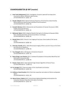
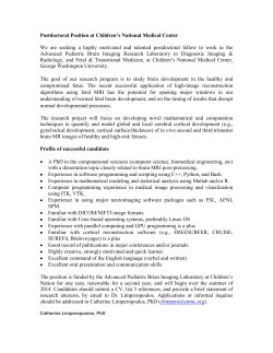
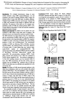
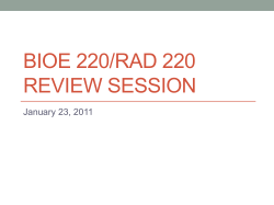
BioMedical Engineering OnLine
This Provisional PDF corresponds to the article as it appeared upon acceptance. Fully formatted
PDF and full text (HTML) versions will be made available soon.
Brain MR image denoising for Rician noise using pre-smooth non-local means
filter
BioMedical Engineering OnLine 2015, 14:2
doi:10.1186/1475-925X-14-2
Jian Yang ([email protected])
Jingfan Fan ([email protected])
Danni Ai ([email protected])
Shoujun Zhou ([email protected])
Songyuan Tang ([email protected])
Yongtian Wang ([email protected])
ISSN
Article type
1475-925X
Research
Submission date
26 July 2014
Acceptance date
19 November 2014
Publication date
9 January 2015
Article URL
http://www.biomedical-engineering-online.com/content/14/1/2
This peer-reviewed article can be downloaded, printed and distributed freely for any purposes (see
copyright notice below).
Articles in BioMedical Engineering OnLine are listed in PubMed and archived at PubMed Central.
For information about publishing your research in BioMedical Engineering OnLine or any BioMed
Central journal, go to
http://www.biomedical-engineering-online.com/authors/instructions/
For information about other BioMed Central publications go to
http://www.biomedcentral.com/
© 2015 Yang et al.
This is an Open Access article distributed under the terms of the Creative Commons Attribution License (http://creativecommons.org/licenses/by/4.0), which
permits unrestricted use, distribution, and reproduction in any medium, provided the original work is properly credited. The Creative Commons Public Domain
Dedication waiver (http://creativecommons.org/publicdomain/zero/1.0/) applies to the data made available in this article, unless otherwise stated.
Brain MR image denoising for Rician noise using
pre-smooth non-local means filter
Jian Yang1
Email: [email protected]
Jingfan Fan1
Email: [email protected]
Danni Ai1
Email: [email protected]
Shoujun Zhou2
Email: [email protected]
Songyuan Tang1*
*
Corresponding author
Email: [email protected]
Yongtian Wang1
Email: [email protected]
1
Beijing Engineering Research Center of Mixed Reality and Advanced Display,
School of Optics and Electronics, Beijing Institute of Technology, Beijing 10081,
China
2
Shenzhen Institutes of Advanced Technology, Chinese Academy of Sciences,
Shenzhen 518055, China
Abstract
Background
Magnetic resonance imaging (MRI) is corrupted by Rician noise, which is image dependent
and computed from both real and imaginary images. Rician noise makes image-based
quantitative measurement difficult. The non-local means (NLM) filter has been proven to be
effective against additive noise.
Methods
Considering the characteristics of both Rician noise and the NLM filter, this study proposes a
frame for a pre-smoothing NLM (PSNLM) filter combined with image transformation. In the
PSNLM frame, noisy MRI is first transformed into an image in which noise can be treated as
additive noise. Second, the transformed MRI is pre-smoothed via a traditional denoising
method. Third, the NLM filter is applied to the transformed MRI, with weights that are
computed from the pre-smoothed image. Finally, inverse transformation is performed on the
denoised MRI to obtain the denoising results.
Results
To test the performance of the proposed method, both simulated and real patient data are
used, and various pre-smoothing (Gaussian, median, and anisotropic filters) and image
transformation [squared magnitude of the MRI, and forward and inverse variance-stabilizing
trans-formations (VST)] methods are used to reduce noise. The performance of the proposed
method is evaluated through visual inspection and quantitative comparison of the peak signalto-noise ratio of the simulated data. The real data include Alzheimer’s disease patients and
normal controls. For the real patient data, the performance of the proposed method is
evaluated by detecting atrophy regions in the hippocampus and the parahippocampal gyrus.
Conclusions
The comparison of the experimental results demonstrates that using a Gaussian presmoothing filter and VST produce the best results for the peak signal-to-noise ratio (PSNR)
and atrophy detection.
Background
Magnetic resonance imaging (MRI) images of the brain have an important role in diagnosing
many neurological diseases, such as Parkinson’s disease, Alzheimer’s disease (AD), brain
tumors, and stroke. Analyzing MRI images can help surgeons make appropriate decisions.
However, MRI noises degrade image quality, which negatively affects image processing and
analysis works, such as registration, segmentation, classification, and visualization. To obtain
reliable analysis results, removing MRI image noises is necessary before further image
processing can be conducted.
The technique of removing noises from images is called “image denoising,” which is an
important image pre-processing step. Although many image denoising methods have been
developed, denoising remains a challenge because these methods produce artifacts and blurry
images [1]. Most denoising methods still cannot provide desirable results [2].
The most commonly used noise model is the additive noise model, that is,
I = I0 + n
(1)
where noise n is independent and Gaussian distribution with zero-mean and known standard
deviation, I0 is the true signal, and I is the observed signal. Most denoising methods have
been developed by using the additive noise model. These methods are classified into two
major categories: spatial filtering and transform domain filtering methods.
Spatial domain techniques directly deal with image pixels. A spatial image filter is an image
operation wherein each pixel or voxel value I(u) is transformed through a function of the
intensities of the pixels or voxels within a neighborhood (u). Traditional spatial image filters
include Gaussian [3], median [4], Wiener [5], diffusion [6], and bilateral filters. Gaussian and
median filters remove noise in a small constant region and blur images. An anisotropic
diffusion filter preserves the edges of images, but erases small features and generates a mask
effect in uniform regions of the denoised images. These denoising methods significantly
remove noise but cause blurred images and add artifacts to the images. A transform domain
image filter transforms images from the space domain into another domain, such as the
frequency and wavelet domains [7], and then processes images in the new domain. The
wavelet thresholding method can significantly reduce noise, but introduces characteristic
artifacts. In this study, we mainly focus on the spatial domain filter.
A non-local mean (NLM) algorithm has been proposed recently [8]. This algorithm provides
good edge-preserving results. Each pixel of the denoised image from the NLM algorithm can
represent the weighted average of all pixels in the noisy image by using a Gaussian function
as the smoothing function. The NLM filter has been proven to be an effective denoising
method, particularly against additive noise.
Many MRI denoising methods have been reported. Gaussian filter smoothing is a key step in
voxel-based morphometry (VBM) analysis [9]. A Wiener filter uses its neighborhood to
estimate its parameters [10]. An anisotropic filter combines local linear minimum mean
squared error (MSE) filters to remove MRI noise [11]. A trilinear filter achieves edgepreserving results by integrating geometric, photometric, and local structural similarities [12].
Noise estimation methods in the wavelet domain are also used in MRI denoising. MRI in the
wavelet domain is decomposed into sub-bands at various scales. Coefficients are processed
with soft or hard thresholding to estimate signal components [13]. The NLM filter is also
used in MRI denoising [14,15].
The noise in the MRI images is modeled according to the coil number in the imaging system.
In the single coil system, the noisy distribution in MRI images can be modeled as a Rician
distribution [16], which assumes that the real part and imaginary part of the MRI image is an
uncorrelated Gaussian distribution with a zero mean and equal variance. While in the multicoil system (parallel MRI), the magnitude of noises follows a non-central Chi distribution
[17] with a sum-of-squares (SoS) reconstruction. The noise in the MRI images acquired from
the generalized auto calibrating partially parallel acquisition (GRAPPA) reconstruction [18]
can be modeled by the non-central Chi distribution. Actually, the Rician distribution is a
special case of the nonCentral Chi distribution. To apply the additive noise model, the
nonCentral Chi distribution should be transformed into the Gaussian distribution in the
transformed space. Therefore, the above-mentioned denoising methods can be applied to the
transformed data. After inverse transformation of the denoising data, the noise is removed
from the MRI images. Many mthods have been proposed to deal with the problem, such as
the local moment distribution based method [19], nonlocal maximum likelihood (NLML)
estimation [20], and the effective variance of noise from the composite magnitude signal of
MR data [20].
In this study, we focus on the single coil system which produces noises with Rician
distribution. To remove noise and apply the additive noise model, Rician noise should be
transformed into an independent Gaussian noise. The squared magnitude correction is widely
used for MRI denoising [13]. The standard deviation of noise is estimated from a dark
uniform background. Recently, a forward and inverse variance-stabilizing transformation
(VST) [21] has been proposed for the Rician distribution. The forward VST removes the
dependency of the noise variance on the observed image, and the inverse VST compensates
the bias in the filtered image.
A frame for a pre-smoothing NLM (PSNLM) filter is proposed in the study. MRI noise is
first transformed into additive noise and then smoothed by a traditional denoising filter
(Gaussian, median, or anisotropic). Next, the weight of the NLM algorithm is calculated from
the smooth image, and noise is removed by the NLM filter. Finally, inverse transformation is
used to obtain accurate results. Squared magnitude transformations, as well as forward and
inverse variance-stabilizing transformations (VST) [21], are adopted to transform noise in the
proposed method.
Methods
The proposed method includes four steps: (1) transformation of noisy MRI, (2) presmoothing of the transformed MRI, (3) noise removal by the NLM filter, and (4) unbiased
correction (inverse transformation) of the denoised image. The block diagram is shown in
Figure 1.
Figure 1 Block diagram of the proposed method.
MRI Model
MRI images are widely used in medical applications because they prevent the formation of
phase artifacts by discarding phase information. MRI is computed from both real and
imaginary images, which are assumed to contain Gaussian distribution noises with zero
means [14]. Thus, noise is image dependent, which follows a Rician distribution, and makes
removing noises difficult. A complex MRI is represented as follows:
z = z real + jzimaginary = ( rcosθ + n1 ) + j ( rsinθ + n 2 )
(2)
where z is the complex MRI; zreal and zimaginary are the real and imaginary components,
respectively, which are independently corrupted by Gaussian white noises n1 and n2,
respectively, with zero mean and standard deviation σ; and r and θ are the magnitude and
phase of the original MRI, respectively.
A measured noisy MRI can be represented as follows:
z =
( rcosθ + n1 ) + ( rsinθ + n 2 )
2
2
(3)
The measured MRI magnitude |z| is under Rician distribution and is represented as follows:
P ( z|r , σ ) =
z
σ
2
e
−
z 2 + R2
2σ 2
 zr 
I0  2 
σ 
(4)
where I0 denotes the modified Bessel function of order zero.
Estimating noise from the measured magnitude |z| of MRI is difficult. The most commonly
used method is to square the magnitude of MRI. Recently, VST is proposed for Rician noise
processing.
The squared magnitude method
Based on Eq. (2), the expectation of |z|2 is given as follows:
2
2
2
E  z  = E ( rcosθ + n1 ) + ( rsinθ + n 2 )  = µr2 + 2σ 2
 


(5)
This equation indicates that the squared magnitude MRI has a 2σ2 noise bias and is image
independent. For an original brain MRI, the background is an empty region with zero
intensity. Thus, σ in the background region can be estimated as follows:
σ=
µ
(6)
2
where µ is the mean intensity of the squared magnitude MRI in the background region. |z|2
can be filtered by using any noise removal method Φ. According to Eq. (4), the unbiased Iu is
estimated as follows:
Φ ( z 2 ) − 2σ 2 if z 2 − 2σ 2 ≥ 0
Iu = 
0
otherwise

(7)
Background of the brain
The background of the brain can be estimated by using any segmentation method. In this
study, the Otsu method [22], which is an automatic image segmentation technique, is adopted
to extract the background region. This algorithm assumes that two classes of pixels or bimodal histogram (e.g., foreground and background) are found in the image and exhaustively
searches for the threshold that maximizes inter-class variance [22,23]. The process includes
median filtering, Otsu segmentation, morphological close operation, and filling the holes in
the image.
If the skulls of T1, T2, and PD are clear, then the mask of the brain is easily segmented as
well as the background that uses the process. An example is shown in Figures 2, 3 and 4.
Figure 2(a) shows the original T1-weighted MRI; Figure 2(b) shows the T1-weighted MRI
with Rician noise; Figure 2(c) presents the result of median filtering; Figure 2(d) provides the
result of the morphological close operation; and Figure 2(e) presents the result after the holes
are filled. Figure 3(a) shows the original T2-weighted MRI; Figure 3(b) shows the T2weighted MRI with Rician noise; Figure 3(c) presents the result of median filtering; Figure
3(d) provides the result of the morphological close operation; and Figure 3(e) presents the
result after the holes are filled. Figure 4(a) shows the original PD-weighted MRI; Figure 4(b)
shows the PD-weighted MRI with Rician noise; Figure 4(c) presents the result of median
filtering; Figure 4(d) provides the result of the morphological close operation; and Figure 4(e)
presents the result after the holes are filled. In these figures, the bright area is the brain
region, whereas the dark area is the background.
Figure 2 An example of extracting background from T1-weighted MRI. (a) the original
T1 weight MRI, (b) the MRI with Rician noise, (c) the result of the median filtering, (d) the
result of the morphological close operation, and (e) the result of the brain region.
Figure 3 An example of extracting background from T2-weighted MRI. (a) the original
T2 weight MRI, (b) the MRI with Rician noise, (c) the result of the median filtering, (d) the
result of the morphological close operation, and (e) the result of the brain region.
Figure 4 An example of extracting background from PD-weighted MRI. (a) the original
PD weight MRI, (b) the MRI with Rician noise, (c) the result of the median filtering, (d) the
result of the morphological close operation, and (e) the result of the brain region.
In many cases, the skull is clear only in the T1-weighted MRI, and its intensities in the T2and PD-weighted MRIs are close to the background. Figure 5 shows the T1-, T2-, and PDweighted MRIs of a patient with meningioma. Figure 5(a) shows the T2-weighted MRI;
Figure 5(b) shows the PD-weighted MRI; and Figure 5(c) shows the T1-weighted MRI. In
such situations, the brain region and the background are easily segmented for the T1weighted image, as shown in Figure 5(d) to (f). Figure 5(d) presents the result of median
filtering; Figure 5(e) provides the result of the morphological close operation; and Figure 5(f)
presents the final result. To obtain the background of the corresponding T2- and PD-weighted
MRIs, we align the T1-weighted MRI to the T2-and PD-weighted MRIs, and transform the
background of the T1-weighted MRI into the T2-and PD-weighted spaces. The transformed
background can be used as the background of the T2- and PD-weighted MRIs. Given that the
images belong to the same person, aligning them is easy. The images are multi-modal;
therefore, a rigid registration with mutual information is selected to align the images [24].
Figure 5 Images of a patient with meningiomais, T2- and PD- weighted MRI are
registered to T1 weighted MRI, which is clear and easy to extract background. The
background region of T1 weighted MRI is also the background region of registered T2- and
PD- weighted MRI. (a) T2 weight MRI, (b) PD weight MRI, and (c) T1 weight MRI, (d) the
result of the median filtering for T1 weight MRI, (d) the result of the corresponding
morphological close operation, and (e) the final result of the background (dark region).
The method of variance-stabilization
This method involves the optimal forward and inverse VSTs for Rician noise. Forward
transformations (f) treat MRI noise as an additive noise with a unitary variance. Thus, noise
can be removed by using the NLM filter. Denoising MRI can be achieved through inverse
transformation (I).
Forward transformations can be represented as follows:
f ( z) =
z2 1
− +a
σ2 2
(8)
2
2
where a is a constant a = f ( zmax ) − zmax / σ − 0.5 . The details can be found in [16]. In this
study, σ is obtained from the background through Eq. (5), as described in the above section.
A denoising method Φ is then applied to f(z) to obtain a noise removal image D.
D = Φ ( f ( z ))
(9)
Inverse transformation is then applied to D to obtain unbiased estimation Iu as follows:
Iu = I ( D ) ≈
σ ( D − a)
2
(10)
( D − a ) + 0.5
2
NLM filter
For a 3D image measuring Nx × Ny × Nz in the NLM filter, the estimated intensity NLM(|z|(i,
j, k)) of voxel (i,j,k) is the weighted average of all voxel intensities in the noisy image |z|,
which is defined as follows:
NLM ( z ( i, j , k ) ) =
N x −1 N y −1 N z −1
∑ ∑ ∑ w ( i, j, k , l , m, n ) z ( l , m, n )
(11)
l =0 m =0 n = 0
where NLM(|z|(i, j, k)) is the intensity of the denoised image at position (i,j,k) through the
NLM filter, |z|(l, m, n) is the intensity of the noisy image at (i,j,k), and w(i, j, k, l, m, n) is the
weighting coefficient that is defined as follows:
w ( i, j , k , l , m, n ) =
1
e
Z ( i, j , k )
where 0 ≤ w ( i, j, k , l , m, n ) ≤ 1,
−
(
)
G a z N i , j ,k − z ( N l ,m ,n )
2
h2
(12)
N x −1 N y −1 N z −1
∑ ∑ ∑ w ( i, j, k , l , m, n ) = 1,
h is the filtering degree. Ni,j,k
l = 0 m = 0 n =0
and Nl,m,n are the blocks centered at voxels (i,j,k) and (l,m,n), respectively, with both blocks
measuring nx × ny × nz; Ga is a Gaussian weighting function with zero mean and standard
deviation, where a is typically set to one; and Z(i, j, k) is a normalizing constant that is
defined as follows:
Z ( i, j , k ) =
N x −1 N y −1 N z −1 −
∑∑∑e
(
) (
G a z Ni, j ,k − z N l ,m ,n
2
)2
h
(13)
l=0 m =0 n = 0
According to the Eq. (10)-(12), to modify each noisy voxel |z|(i, j, k), its neighborhood
|z|(Ni,j,k) is compared with other noisy voxel’s neighborhood |z|(Nl,m,n) in the entire image. It
needs huge computation. Considering the computational efficiency, usually the search
window is selected to be a much smaller than the size of the entire image and is sx × sy × sz.
The Pre-smooth Non-local Means Filter (PSNLM)
Before using the NLM filter, MRI |z| is first transformed into It via forward transformation f
(squared magnitude or variance stabilization). Subsequently, It is smoothed by a traditional
filter S (Gaussian, median, or anisotropic) to become Is . When the NLM filter is used to
remove noise, the weight and normalizing constant are calculated from Is as follows:
It = f ( z ) , I s = S ( It )
(14)
−
1
w ( i, j, k , l , m, n ) =
e
Z(i, j, k )
Z ( i, j , k ) = ∑ l =0
N x −1
∑
N y −1
m =0
∑
(
h
N z −1 −
n =0
)
G a I s N i , j , k − I s ( Nl , m , n )
(
2
(15)
2
)
G a I s N i , j ,k − I s ( N l ,m ,n )
2
(16)
h2
e
An unbiased estimation is obtained through inverse transformation of the PSNLM result.
PSNLM1 and PSNLM2 are used to represent squared magnitude and VST, respectively.
( ) − 2σ

 PSNLM I s
PSNLM1 = 

0

2
2
( ) − 2σ
if PSNLM I s
2
2
≥0
(17)
otherwise

 I2 1

s

−
+
−
a
a

 σ2 2





2
σ  PSNLM 
PSNLM2 =


2


 I2 1

 PSNLM  s 2 − + a  − a  + 0.5
 σ



2




(18)
The summary of PSNLM is listed in Table 1.
Table 1 Summary of the PSENLM
PSENLM1
PSENLM2
(1) Extract background
(1) Transform noisy image by the forward variance-stabilization
transformation
(2) Smooth the transformed image
(3) Compute the weigh term from the smoothed image
(4) Obtained final result by the inverse variance-stabilization
transforming of the NLM denoising result
(2) Compute the noise variance σ2 according Eq. (5)
(3)Compute the squared magitude of noisy image
(4)Smooth the squared magitude of noisy image
(5) Compute the weigh term from the smoothed image
(6) Correct bias by subtracting 2σ2 from the NLM denoising result.
The final result is obtained by squared root of the bias correction
Evaluation
For the simulated data, the results are measured quantitatively by the peak signal-to-noise
ratio (PSNR), which is a commonly used objective metrics, and visual inspection. PSNR is
defined as follows [25]:
C2
PSNR = 10log10
MSE
(19)
where C is the maximum intensity in which the image can be given. MSE between the final
denoised image and the original image is defined as follows:
MSE =
1
Nx × N y × Nz
∑ ∑ ∑ ( PSNLM 1( i, j, k ) − r ( i, j, k ) )
MSE =
1
Nx × N y × Nz
∑ ∑ ∑ ( PSNLM 2 ( i, j, k ) − r ( i, j, k ) )
N x −1
N y −1
N z −1
i =0
j =0
k =0
N x −1
N y −1
N z −1
i =0
j =0
k =0
2
2
(20)
(21)
where PSNLM1(i, j, k) and PSNLM2(i, j, k) are the voxels of PSNLM1 and PSNLM2,
respectively, at position (i, j, k); and r(i, j, k) is the original MRI at position (i, j, k). A large
PSNR indicates good results.
For real patient data, the performance of the proposed method in detecting brain atrophy
among patients with AD is evaluated by using VBM [9,26]. In VBM studies, all individual
brain images are spatially normalized onto template space through a registration algorithm.
Based on the estimated deformation field, each brain morphometry information can be
measured by using a Jacobian map, which reflects regional volumetric changes that are
compared with the template image. Subsequently, voxel-wise group analysis is performed by
using SPM software to detect brain atrophy [27].
Experiment data
The experiment data include both simulated and real patient data. The 3D-simulated MRI
images that are used in the experiments are downloaded from the BrainWeb database [2]. The
simulated T1-, T2-, and PD-weighted MRI images without noise are downloaded. The size of
each image is 181 × 217 × 181 and the intensity is 256 bins. Rician noise is simulated
according to Eq. (2), with n1 ~ N(0, σ), n2 ~ N(0, σ), θ = 0, and r is a an image without noise,
which can be taken as the ground truth. Various levels of noise (percent %) are added to the
three MRI images.
σ = percent% × t
(22)
where t is the intensity of the brightest tissue, which is 150, 250, and 255 for T1-, T2-, and
PD-weighted MRI images, respectively, with 256 bins. The noisy image is given as follows:
z =
( r + σ × randn ( size ( r ) ) ) + ( σ × randn ( size ( r ) ) )
2
2
(23)
In this case, randn(size(r)) produces data with the same size as the ground truth image, and
the mean and standard deviation of the data are 0 and 1, respectively. The real patient data
that are used in this study are downloaded from the Alzheimer’s Disease Neuroimaging
Initiative (ADNI) database [27], which includes many T1-weighted MRI images of AD
patients and normal controls (NC). To test the performance of the proposed method, 20 NCs
and 20 AD patients with T1-weighted MRI images of the baseline are randomly selected
from the database.
Results and discussion
The experimental results are obtained from both simulated and real patient data.
Simulated data
For the simulated data, several noise levels, namely, 9%, 13%, 17%, and 21% are added into
T1-, T2-, and PD-weighted MRI images. Examples of T1-, T2-, and PD-weighted MRI
images with 17% noise are shown in Figures. 6, 7 and 8, respectively. Figure 6(a) shows the
original T1-weighted MRI image, whereas Figure 6(b) shows the corresponding noisy MRI
image. Figure 7(a) shows the original T2-weighted MRI image, whereas Figure 7(b) shows
the corresponding noisy T2-weighted MRI image. Figure 8(a) shows the original PDweighted MRI image, whereas Figure 8(b) shows the corresponding noisy MRI image. In this
study, squared magnitude and VST are used to transform noisy MRI image into additive
noise. Figure 6(c) shows the squared magnitude noisy T1-weighted MRI image, whereas
Figure 6(d) shows the forward VST of the noisy T1-weighted MRI image. Figure 6(c) shows
the squared magnitude noisy T2-weighted MRI image, whereas Figure 7(d) shows the
forward VST of the noisy T2-weighted MRI image. Figure 8(c) shows the squared magnitude
noisy PD-weighted MRI image, whereas Figure 8(d) shows the forward VST of the noisy
PD-weighted MRI image.
Figure 6 An example of T1 image: (a) original T1 weighted MRI, (b) 17% noisy T1
weighted MRI, (c) squared magnitude of the noisy T1 weighted MRI, (d) the forward
variance-stabilization transformation of the noisy T1 weighted MRI.
Figure 7 An example of T2 image: (a) original T2 weighted MRI, (b) 17% noisy T2
weighted MRI, (c) squared magnitude of the noisy T2 weighted MRI, (d) the forward
variance-stabilization transformation of the noisy T1 weighted MRI.
Figure 8 An example of PD image: (a) original PD weighted MRI, (b) 17% noisy PD
weighted MRI, (c) squared magnitude of the noisy PD weighted MRI, (d) the forward
variance-stabilization transformation of the noisy PD weighted MRI.
Moreover, several filters are used to pre-smooth images. In this study, common filters, such
as Gaussian, median, and anisotropic filters, are used to pre-smooth MRI images. The NLM
algorithm has three parameters: patch size, search window size sx × sy × sz, and filtering
degree h. In many NLM-based MRI denoising cases, patch size is set as 5 × 5 × 5, and search
window size is set as 11 × 11 × 11 for MRI images with a voxel size of 1 × 1 × 1 mm3 [13].
Thus, the same parameters are used in this study. h is typically set as proportional to the noise
level of the image. In our experiments, different h values are tested, and we selected the h
value that produces the largest PSNR. For comparison, the PSNR of different methods are
calculated. These methods include the original NLM algorithm, unbiased correction (UNLM)
by the squared magnitude, as well as VST, PSNLM1, and PSNLM2 with Gaussian, median,
and anisotrpic filters, respectively.
Comparison of PSNR
Figures 9, 10 and 11 show the comparisons of the experiment results with PSNR. Figure 9
shows the PSNR of the T1-weighted MRI image at different noise levels. Figure 9(a)
includes the PSNR of the original NLM, UNLM with squared magnitude, and PSNLM1 with
Gaussian, median, and anisotropic filters. The curve of the PSNLM1 with a Gaussian filter is
at the top. Figure 9(b) includes the PSNR of the original NLM, UNLM with VST, and
PSNLM2 with Gaussian, median, and anisotropic filters. The curve of the PSNLM2 with a
Gaussian filter is also at the top. The PSNR of the original NLM algorithm are at the bottom
of both figures. The PSNR curves of the UNLM and PSNLM with median and anisotropic
filters are between that of the PSNLM with a Gaussian filter and NLM. The proposed method
can improve the denoising results. Pre-smoothing with a Gaussian filter achieves the best
results. Figure 9(c) shows the PSNR curves of the PSNLM2 and PSNLM1with a Gaussian
filter. The PSNR of PSNLM2 is larger than that of PSNLM1. This result indicates that the
proposed method with VST and a Gaussian filter performs the best. Figure 9(d) shows that
the PSNR of the UNLM with VST is larger than that of the UNLM with the squared
magnitude. Thus, VST is the better choice between the two.
Figure 9 T1 weighted MRI: (a) PSNR of the original NLM, UNLM with squared
magnitude, and PSNLM1 with Gaussian, median, and anisotropic filters, (b) PSNR of
the original NLM, UNLM with VST, and PSNLM2 with Gaussian, median, and
anisotropic filters. (c) PSNR of PSNLM with Gaussian filter, and (d) PSNR of ULM with
VST and squared magnitude.
Figure 10 PD weighted MRI, (a) PSNR of the original NLM, UNLM with squared
magnitude, and PSNLM1 with Gaussian, median, and anisotropic filters, (b) PSNR of
the original NLM, UNLM with VST, and PSNLM2 with Gaussian, median, and
anisotropic filters. (c) PSNR of PSNLM with Gaussian filter, and (d) PSNR of ULM with
VST and squared magnitude
Figure 11 T2 weighted MRI, (a) PSNR of the original NLM, UNLM with squared
magnitude, and PSNLM1 with Gaussian, median, and anisotropic filters, (b) PSNR of
the original NLM, UNLM with VST, and PSNLM2 with Gaussian, median, and
anisotropic filters. (c) PSNR of PSNLM with Gaussian filter, and (d) PSNR of ULM with
VST and squared magnitude
Figures 10 and 11 show the PSNR of the PD- and T2-weighted MRI images with different
noise levels. The results are similar to that of the T1-weighted MRI image. The PSNR curves
with a Gaussian filter are at the top, as shown in Figure 10(a) and (b) for the PD-weighted
MRI images and Figure 11(a) and (b) for the T2-weighted MRI images. Figures 10(c) and
11(c) show the PSNR of the PSNLM1 and PSNLM2 with a Gaussian filter for the PD- and
T2-weighted MRI images. The two curves are extremely close in Figure 10(c). The PSNR of
PSNLM2 is slightly larger than that of PSNLM1. In Figure 11(c), the PSNR of PSNLM2 is
larger than that of PSNLM1. Figures 10(d) and 11(d) show the PSNR of the UNLM with
VST and with the squared magnitude, respectively. The curves are extremely close at a low
noise level for the PD-weighted MRI image [Figure 10(d)] and at a high noise level for the
T2-weighted MRI image.
Comparison by visual inspection
Figure 12 shows the enlarged regions of the experimental results on the T1-weighted MRI
image. Figure 12(a) shows an enlarged region of the original MRI, and Figure 12(b) shows
noisy MRI with 17% Rician noise. Figure 12(c) presents the result of the original NLM. The
edges are obviously blurred. Figure 12(d) and (h) present the results of the UNLM with the
squared magnitude and VST, respectively. Figure 12(h) is clearer than Figure 12(d).
Although both results are better than that of the original NLM algorithm, the images are still
blurred. Figure 12(e) to (g) present the results of the PSNLM1 with median, Gaussian, and
anisotropic filters, respectively, whereas Figure 12(i) to (k) present the results of the
PSNLM2 with median, Gaussian, and anisotropic filters, respectively. All results are
significantly improved compared with Figure 12(d) and (h). However, some artifacts are
observed in Figure 12(e), (g), (i), and (k). Figure 12(f) and (j) show that the results are
extremely close to and similar to those of the original image. Nevertheless, the result in
Figure 12(j) is slightly better than those in the other figures. Figure 13 is another enlarged
region of the experimental results on the T1-weighted MRI image. Comparably, there are
some artifacts in Figure 13(e),(f),(g) and (i), Figure 13(c),(d) and (h) are slight blurred, while
Figure 13 (j) and (k) are clearer than the others. It is obvious that the results of PSNLM2 with
Gaussian and median filters are better than the other methods.
Figure 12 Comparison of experiment results on T1-weighted MRI. (a) original MRI, (b)
noisy MRI with 17% Rician noise, (c) results of the original NLM filter, (d) results of the
UNLM with squared magnitude transformation, (e) results of the PSNLM1 with median
filter, (f) results of the PSNLM1 with Gaussian filter, (g) results of the PSNLM1 with
anisotropic filter, (h) results of the UNLM with VST, (i) results of the PSNLM2 with median
filter, (j) results of the PSNLM2 with Gaussian filter, (k) results of the PSNLM2 with
anisotropic filter.
Figure 13 Comparison of experiment results on T1-weighted MRI. (a) original MRI, (b)
noisy MRI with 17% Rician noise, (c) results of the original NLM filter, (d) results of the
UNLM with squared magnitude transformation, (e) results of the PSNLM1 with median
filter, (f) results of the PSNLM1 with Gaussian filter, (g) results of the PSNLM1 with
anisotropic filter, (h) results of the UNLM with VST, (i) results of the PSNLM2 with median
filter, (j) results of the PSNLM2 with Gaussian filter, (k) results of the PSNLM2 with
anisotropic filter.
Figure 14 presents the results on the PD-weighted MRI image with 17% Rician noise. Figure
14(a) shows an enlarged region of the original MRI image, and Figure 14(b) shows the noisy
MRI image. Figure 14(c) presents the result of the original NLM. Figure 14(d) and (h)
present the results of the UNLM with the squared magnitude and VST, respectively. Figure
14(e) to (g) present the results of the PSNLM1 with median, Gaussian, and anisotropic filters,
respectively. Figure 14(i) to (k) present the results of the PSNLM2 with median, Gaussian,
and anisotropic filters, respectively. It is obvious that Figure 14(c), (d) and (h) are blurred,
while the pre-smooth technique significantly improves the result, as can be seen in Figure
14(j).
Figure 14 Comparison of experiment results on PD-weighted MRI. (a) original MRI, (b)
noisy MRI with 17% Rician noise, (c) results of the original NLM filter, (d) results of the
UNLM with squared magnitude transformation, (e) results of the PSNLM1 with median
filter, (f) results of the PSNLM1 with Gaussian filter, (g) results of the PSNLM1 with
anisotropic filter, (h) results of the UNLM with VST, (i) results of the PSNLM2 with median
filter, (j) results of the PSNLM2 with Gaussian filter, (k) results of the PSNLM2 with
anisotropic filter.
Figure 15 is another enlarged region of the experiment results on the PD-weighted MRI
image. It is obvious that Figure 15(c),(d) and (h) are, to some extent, blurred. While the
proposed pre-smooth technique greatly improves the result, as can be seen in Figure 15(j).
Figure 15 Comparison of experiment results on PD-weighted MRI. (a) original MRI, (b)
noisy MRI with 17% Rician noise, (c) results of the original NLM filter, (d) results of the
UNLM with squared magnitude transformation, (e) results of the PSNLM1 with median
filter, (f) results of the PSNLM1 with Gaussian filter, (g) results of the PSNLM1 with
anisotropic filter, (h) results of the UNLM with VST, (i) results of the PSNLM2 with median
filter, (j) results of the PSNLM2 with Gaussian filter, (k) results of the PSNLM2 with
anisotropic filter.
Figure 16 presents the results on the T2-weighted MRI image with 17% Rician noise. Figure
16(a) shows an enlarged region of the original MRI image, and Figure 16(b) shows the noisy
MRI image. Figure 10(c) presents the result of the original NLM. Figure 16(d) and (h)
present the results of the UNLM with the squared magnitude and VST, respectively. Figure
16(e) to (g) present the results of the PSNLM1 with median, Gaussian, and anisotropic filters,
respectively. Figure 16(i) to (k) present the results of the PSNLM2 with median, Gaussian,
and anisotropic filters, respectively. The result presented in Figure 16(c) exhibits the worst
performance, and also, considerable noise occurs in Figure 16(d) and (h). Serious artifacts are
observed in Figure 16(e), (i) and (g). Figure 16(f) and (k) are more blur than Figure 16(j).
Figure 17 shows another enlarged region of the experiment results on the T2-weighted MRI
image. The results are similar to those in Figure 16. And we can confirm that Figure 17(j) is
the best.
Figure 16 Comparison of experiment results on T2-weighted MRI. (a) original MRI, (b)
noisy MRI with 17% Rician noise, (c) results of the original NLM filter, (d) results of the
UNLM with squared magnitude transformation, (e) results of the PSNLM1 with median
filter, (f) results of the PSNLM1 with Gaussian filter, (g) results of the PSNLM1 with
anisotropic filter, (h) results of the UNLM with VST, (i) results of the PSNLM2 with median
filter, (j) results of the PSNLM2 with Gaussian filter, (k) results of the PSNLM2 with
anisotropic filter
Figure 17 Comparison of experiment results on T2-weighted MRI. (a) original MRI, (b)
noisy MRI with 17% Rician noise, (c) results of the original NLM filter, (d) results of the
UNLM with squared magnitude transformation, (e) results of the PSNLM1 with median
filter, (f) results of the PSNLM1 with Gaussian filter, (g) results of the PSNLM1 with
anisotropic filter, (h) results of the UNLM with VST, (i) results of the PSNLM2 with median
filter, (j) results of the PSNLM2 with Gaussian filter, (k) results of the PSNLM2 with
anisotropic filter
Real patient data
The brains of AD patients are atrophic, particularly at the hippocampus and the
parahippocampal gyrus. Atrophy in these regions can be used as an early biomarker of AD
[28]. To test atrophy degree in the brain, all AD and NC data are first denoised and then
normalized to the Automated Anatomical Labeling template [29], which is a digital human
brain atlas with labeled regions. These regions indicate brain structures. Given that the
Jacobian map of the deformation field includes information on the local properties of the
deformation field that can be used to detect volume changes, Jacobian logarithms are
calculated such that the expansion and compression of the brain are scaled equally [30]. LogJacobians are calculated at each voxel in the volume to produce a map of the local expansion
and compression of the brain. The Jacobian maps are smoothed by using smoothing kernels
that measure 6 mm full-width at half-maximum for each of the 40 samples. By using SPM
software [23], paired t-test is performed on the Jacobian maps of the AD and NC groups. An
equal p value (p =0.05) is used to compare the t-score obtained by the different denoising
methods. The ratios of the detected atrophy region to the region of the hippocampus and the
parahippocampal gyrus are listed in Table 2. The minimum ratio is 9.93, which is obtained
from the original image. The maximum ratio is 58.69, which is obtained from the image
denoised by the PSNLM2 with a Gaussian filter. The ratio of image denoising by the NLM
filter is 55.98, which is only larger than that of the original image. This result indicates that
image denoising significantly increases the ratios of the detected atrophy region to the region
of the hippocampus and the parahippocampal gyrus. The transformation of Rician noise into
additive noise can further increase the ratios. The PSNLM2 with a Gaussian filter is the best
method for detecting atrophy regions.
Table 2 The ratios of the detecting atrophy region and the region of hippocampus and
parahippocampal gyrus
1
2
3
4
5
6
7
8
9
10
9.93
55.98
57.66
58.55
56.03
57.74
57.52
57.09
58.69
57.76
1. Original image.
2. Image denoising by the nlm.
3. Image denoising by the unlm with squared magnitude transformation.
4. Image denoising by the unlm with VST.
5. Image denoising by the PSNLM1 with anisotropic filter.
6. Image denoising by the PSNLM1 with gaussian filter.
7. Image denoising by the PSNLM1 with median filter.
8. Image denoising by the PSNLM2 with anisotropic filter.
9. Image denoising by the PSNLM2 with gaussian filter.
10. Image denoising by the PSNLM2 with median filter.
Moreover, the proposed method is compared with other recently developed methods,
including Rician image denoising, linear minimum mean square error (LMMSE) estimator
[31] and total variation minimization (TV) [32]. A series of 2D T1 weighted MRI knee
images are utilized to illustrate the performance of the proposed method. The image size is
383×420. Table 3 lists the results of the IMMSE, TV and PSNLM2, it can be seen that the
noise level of the Rician noise is from 2% to 20%. While the proposed PSNLM2 method has
the largest PSNR at each level of noise.
Table 3 The PSNR of noisy image, results of LMMSE, TV and PSNLM2
Noisy
LMMSE
TV
PSNLM2
2%
4%
6%
8%
10%
12%
14%
16%
18%
20%
33.33
36.38
36.87
37.60
27.48
32.41
33.19
33.93
24.19
30.25
30.30
31.78
21.86
28.32
28.53
30.12
20.64
27.01
27.21
29.14
19.42
25.48
25.63
27.93
18.74
25.38
25.18
26.92
17.86
24.45
24.69
26.13
17.56
23.16
23.36
25.34
16.91
22.34
22.40
24.52
The larger PSNR indicate the better performance. The maximun PSNR is listed by symbol
bold at each noise level.
Conclusion
In this study, a PSNLM frame combined with image transformation is proposed for MRI
denoising. After the Rician noise in MRI is transformed to the additive noise, the NLM filter
is applied to the transformed image with weights computed from the pre-smooth image. The
final denoising image is obtained from the inverse transformation of the NLM denoising
result. Experiments are performed on the simulated data of the T1-, T2-, and PD-weighted
MRI images that are downloaded from the BrainWeb database and real data (T1-weighted
MRI images) downloaded from ADNI. Many traditional filters are tested as pre-smooth
filters. In this paper, only the results using Gaussian, median, and anisotropic filters are
presented because others such as trilateral filter and wavelet filter produce worse results. The
proposed method is automatic and robust since it improves the denoising results greatly in all
the experiments. One challenge problem for the proposed method is that it is comparably
time consuming, which costs about 15 minutes on the image size 181×217×181 with 10
threads on the Dell server. The reason is that the image transformation of the NLM takes
heavy computation. Recently, many works have been proposed with respect to decrease the
computation time of the NLM, such as the FFT transformation [33], which is about fifty
times faster than the original non-local algorithm and can reach the clinic application. The
experiment results indicate that using the Gaussian pre-smoothing filter and VST produces
the best results for the peak signal-to-noise ratio (PSNR) and atropy detection.
Competing interests
The authors declare that they have no competing interests.
Authors’ contributions
YJ conceived of the study and drafted the manuscript. FJF suggested the algorithm, and
implemented the algorithm. ADN and ZSJ performed the acquisition of the images and
expressed opinions on the evaluation metric. TSY participated in the design of the study,
drew a part of figures and performed the image analysis. WYT helped to draft the manuscript
and expressed opinions on the overall framework of the manuscript. All authors have read
and approved the final manuscript.
Acknowledgements
This research was supported by the National Basic Research Program of China
(2013CB328806), the Key Projects in the National Science & Technology Pillar Program
(2013BAI01B01), the National Hi-Tech Research and Development Program
(2013AA013703), and the National Natural Science Foundation of China (61179020).
References
1. Gupta K, Gupta SK: Image Denoising techniques-a review paper. IJITEE 2013, 2:6–9.
2. Buades A, Coll B, Morel J-M: A review of image denoising algorithms, with a new one.
Multiscale Model Simulat 2005, 4:490–530.
3. Haddad RA, Akansu AN: A class of fast Gaussian binomial filters for speech and
image processing. Signal Process IEEE Trans 1991, 39:723–727.
4. Arias-Castro E, Donoho DL: Does median filtering truly preserve edges better than
linear filtering? Ann Stat 2009, 37:1172–1206.
5. Lim JS: Two-dimensional signal and image processing. NJ, Prentice Hall, Englewood
Cliffs: MIT, Cambridge, MA, Englewood Cliffs; 1990.
6. Perona P, Malik J: Scale-space and edge detection using anisotropic diffusion. IEEE
Trans Pattern Anal Mach Intell 1990, 12:629–639.
7. Fowler JE: The redundant discrete wavelet transform and additive noise. IEEE Signal
Process Lett 2005, 12:629–632.
8. Buades A, Coll B, Morel J-M: Computer vision and pattern recognition. In 2005 CVPR
2005 IEEE Computer Society Conference on. IEEE. ; 2005:60–65.
9. Ashburner J, Friston KJ: Voxel-based morphometry—the methods. Neuroimage 2000,
11:805–821.
10. Martin-Fernandez M, Alberola-Lopez C, Ruiz-Alzola J, Westin C-F: Sequential
anisotropic Wiener filtering applied to 3D MRI data. Magn Reson Imaging 2007, 25:278–
292.
11. Krissian K, Aja-Fernández S: Noise-driven anisotropic diffusion filtering of MRI.
IEEE Trans Image Process 2009, 18:2265–2274.
12. Wong W, Chung A: Trilateral filtering: a non-linear noise reduction technique for
MRI. In International Society for Magnetic Resonance in Medicine. 2004:2218.
13. Nowak RD: Wavelet-based Rician noise removal for magnetic resonance imaging.
IEEE Trans Image Process 1999, 8:1408–1419.
14. Manjón JV, Carbonell-Caballero J, Lull JJ, García-Martí G, Martí-Bonmatí L, Robles M:
MRI denoising using non-local means. Med Image Anal 2008, 12:514–523.
15. Liu H, Yang C, Pan N, Song E, Green R: Denoising 3D MR images by the enhanced
non-local means filter for Rician noise. Magn Reson Imaging 2010, 28:1485–1496.
16. Gudbjartsson H, Patz S: The Rician distribution of noisy MRI data. Magn Reson Med
1995, 34:910–914.
17. Constantinides CD, Atalar E, McVeigh E: Signal-to-noise measurements in magnitude
images from NMR phased arrays. In Engineering in Medicine and Biology Society, 1997
Proceedings of the 19th Annual International Conference of the IEEE. 1997:456–459.
18. Aja-Fernández S, Tristán-Vega A, Hoge WS: Statistical noise analysis in GRAPPA
using a parametrized noncentral Chi approximation model. Magn Reson Med 2011,
65:1195–1206.
19. Aja-Fernández S, Tristán-Vega A, Alberola-López C: Noise estimation in single-and
multiple-coil magnetic resonance data based on statistical models. Magn Reson Imaging
2009, 27:1397–1409.
20. Aja-Fernández S, Brion V, Tristán-Vega A: Effective noise estimation and filtering
from correlated multiple-coil MR data. Magn Reson Imaging 2013, 31:272–285.
21. Foi A: Noise estimation and removal in mr imaging: The variance-stabilization
approach. In Biomedical Imaging: From Nano to Macro, 2011 IEEE International
Symposium on. IEEE. 2011:1809–1814.
22. Qu Z, Zhang L: Research on image segmentation based on the improved Otsu
algorithm. In Intelligent Human-Machine Systems and Cybernetics (IHMSC), 2010 2nd
International Conference on. IEEE. 2010:228–231.
23. Otsu N: A threshold selection method from gray-level histograms. Automatica 1975,
11:23–27.
24. Pluim JP, Maintz JA, Viergever MA: Mutual-information-based registration of
medical images: a survey. IEEE Trans Med Imaging 2003, 22:986–1004.
25. Huynh-Thu Q, Ghanbari M: Scope of validity of PSNR in image/video quality
assessment. Electron Lett 2008, 44:800–801.
26. Ashburner J, Csernansk JG, Davatzikos C, Fox NC, Frisoni GB, Thompson PM:
Computer-assisted imaging to assess brain structure in healthy and diseased brains.
Lancet Neurol 2003, 2:79–88.
27. Jack CR, Bernstein MA, Fox NC, Thompson P, Alexander G, Harvey D, Borowski B,
Britson PJ, Whitwell LJ, Ward C: The Alzheimer’s disease neuroimaging initiative
(ADNI): MRI methods. J Magn Reson Imaging 2008, 27:685–691.
28. Echávarri C, Aalten P, Uylings H, Jacobs H, Visser P, Gronenschild E, Verhey F,
Burgmans S: Atrophy in the parahippocampal gyrus as an early biomarker of
Alzheimer’s disease. Brain Struct Funct 2011, 215:265–271.
29. Tzourio-Mazoyer N, Landeau B, Papathanassiou D, Crivello F, Etard O, Delcroix N,
Mazoyer B, Joliot M: Automated anatomical labeling of activations in SPM using a
macroscopic anatomical parcellation of the MNI MRI single-subject brain. Neuroimage
2002, 15:273–289.
30. Christensen GE, Song JH, Lu W, El Naqa I, Low DA: Tracking lung tissue motion and
expansion/compression with inverse consistent image registration and spirometry. Med
Phys 2007, 34:2155–2163.
31. Aja-Fernandez S, Alberola-Lopez C, Westin CF: Noise and signal estimation in
magnitude MRI and Rician distributed images: a LMMSE approach. IEEE Trans Image
Process 2008, 17(8):1383–1398.
32. Getreuer P, Tong M, Vese LA: A Variational Model for the Restoration of MR Images
Corrupted by Blur and Rician Noise. Advances in Visual Computing, Lecture Notes in
Computer Science. 2011. 6938:686–698.
33. Wang J, Guo Y, Ying Y: Fast non-local algorithm for image denoising. In Image
Processing, 2006 IEEE International Conference. 2006:1429–1432.
Figure 1
Figure 2
Figure 3
Figure 4
Figure 5
Figure 6
Figure 7
Figure 8
Figure 9
Figure 10
Figure 12
Figure 13
Figure 14
Figure 16
Figure 17