
The Mechanics of Soils and Foundations, Second Edition
The Mechanics of Soils and Foundations
Also available from Taylor & Francis
Introductory Geotechnical Engineering
Y.S. Fang et al.
Geotechnical Engineering 2nd ed
R. Lancellotta
Hb: ISBN 9780415304016
Pb: ISBN 9780415304023
Hb: ISBN 9780415420037
Pb: ISBN 9780415420044
Pile Design & Construction Practice 5th ed
M. Tomlinson et al.
Hb: ISBN 9780415385824
Piling Engineering
W.G.K. Fleming et al.
Hb: ISBN 9780415266468
Foundations of Geotechnical Engineering
I. Jefferson et al.
Hb: ISBN 9780415272407
Pb: ISBN 9780415272414
Decoding Eurocode 7
A. Bond et al.
Hb: ISBN 9780415409483
Geotechnical Physical Modelling
C. Leung et al.
Hb: ISBN 9780415420174
Information and ordering details
For price availability and ordering visit our website www.tandfbuiltenvironment.com/
Alternatively our books are available from all good bookshops.
The Mechanics of Soils
and Foundations
Second Edition
John Atkinson
First published 1993 by McGraw-Hill
Second edition published 2007 by Taylor & Francis
2 Park Square, Milton Park, Abingdon, Oxon OX14 4RN
Simultaneously published in the USA and Canada
by Taylor & Francis
270 Madison Avenue, New York, NY 10016, USA
Taylor & Francis is an imprint of the Taylor & Francis Group, an informa business
This edition published in the Taylor & Francis e-Library, 2007.
“To purchase your own copy of this or any of Taylor & Francis or Routledge’s
collection of thousands of eBooks please go to www.eBookstore.tandf.co.uk.”
© 2007 John Atkinson
All rights reserved. No part of this book may be reprinted or reproduced or
utilised in any form or by any electronic, mechanical, or other means, now known
or hereafter invented, including photocopying and recording, or in any
information storage or retrieval system, without permission in writing from the
publishers.
The publisher makes no representation, express or implied, with regard to the
accuracy of the information contained in this book and cannot accept any legal
responsibility or liability for any efforts or omissions that may be made.
British Library Cataloguing in Publication Data
A catalogue record for this book is available from the British Library
Library of Congress Cataloging-in-Publication Data
Atkinson, J.H.
The mechanics of soils and foundations/John Atkinson. – 2nd ed.
p. cm.
Includes bibliographical references and Index.
ISBN 978-0-415-36256-6 (alk. paper) – ISBN 978-0-415-36255-9 (alk. paper)
1. Soil mechanics. 2. Foundations. 3. Slopes (Soil mechanics) I. Title.
TA710.A786 2007
624.1 5–dc22
2006049709
ISBN 0-203-01288-7 Master e-book ISBN
ISBN 10: 0-415-36255-5 (hbk)
ISBN 10: 0-415-36256-3 (pbk)
ISBN 10: 0-203-01288-7 (ebk)
ISBN 13: 978-0-415-36255-9 (hbk)
ISBN 13: 978-0-415-36256-6 (pbk)
ISBN 13: 978-0-203-01288-8 (ebk)
Contents
Preface to the 1st edition
Preface to the 2nd edition
A note on units
Greek alphabet
Glossary of symbols
Some simple experiments to illustrate geotechnical engineering
1
Introduction to geotechnical engineering
1.1
1.2
1.3
1.4
1.5
1.6
1.7
1.8
1.9
2
1
What is geotechnical engineering? 1
Principles of engineering 3
Fundamentals of mechanics 3
Material behaviour 4
Basic characteristics of soils 7
Basic forms of geotechnical structure 7
Factors of safety and load factors 8
Standards and codes of practice 10
Summary 10
Further reading 11
Basic mechanics
2.1
2.2
2.3
2.4
2.5
2.6
2.7
2.8
2.9
xiv
xvii
xix
xx
xxi
xxvi
Introduction 12
Stresses and strains 12
Plane strain and axial symmetry 14
Rigid body mechanics 14
Analysis of stress 16
Analysis of strain 16
Stress ratio and dilation 18
Slip surfaces 20
Summary 21
Worked examples 21
Further reading 23
12
vi
3
Contents
Essentials of material behaviour
3.1
3.2
3.3
3.4
3.5
3.6
3.7
3.8
3.9
3.10
3.11
3.12
4
5
53
Description and classification 53
Description of soils 53
Soil particle sizes, shapes and gradings 54
Properties of fine-grained soils 56
Specific volume, water content and unit weight 57
Limits of consistency 58
Current state 60
Origins of soils 61
Summary 62
Worked examples 62
References 65
Further reading 65
Pore pressure, effective stress and drainage
6.1
6.2
6.3
44
Introduction 44
The Earth’s crust 44
Geological processes 46
Stratigraphy and the age of soils and rocks 46
Depositional environments 47
Recent geological events 50
Importance of geology in geotechnical engineering 52
Further reading 52
Classification of soils
5.1
5.2
5.3
5.4
5.5
5.6
5.7
5.8
5.9
6
Stress–strain behaviour, stiffness and strength 24
Choice of parameters for stress and strain 25
Strength 28
Brittle and ductile 30
Stiffness 31
Strength, stiffness and rigidity 32
Constitutive equations 33
Elasticity 34
Perfect plasticity 35
Combined elasto–plastic behaviour 37
Time and rate effects 41
Summary 42
Worked examples 42
Further reading 43
The structure of the Earth
4.1
4.2
4.3
4.4
4.5
4.6
4.7
24
Introduction 66
Stress in the ground 66
Groundwater and pore pressure 67
66
Contents
6.4
6.5
6.6
6.7
6.8
6.9
6.10
6.11
7
7.7
7.8
7.9
7.10
7.11
8
105
Introduction 105
Isotropic compression and swelling 105
Overconsolidation and yield stress ratio 108
State of soils on the wet side and on the dry side of critical 110
One-dimensional compression and swelling 112
Horizontal stress in one-dimensional loading 114
Summary 116
Worked examples 116
Further reading 118
Critical state strength of soil
9.1
9.2
9.3
9.4
9.5
9.6
85
Purposes of laboratory tests 85
Standard tests and specifications 86
Basic classification tests 86
Measurement of coefficient of permeability 88
Principal features of soil loading tests 90
One-dimensional compression and consolidation
(oedometer) tests 92
Shear tests 92
Conventional triaxial compression tests 93
Hydraulic triaxial cells – stress path tests 96
Comments on soil testing 98
Summary 99
Worked examples 99
Further reading 104
Compression and swelling
8.1
8.2
8.3
8.4
8.5
8.6
8.7
9
Suctions in saturated soil 68
Effective stress 70
Importance of effective stress 71
Demonstrations of effective stress 72
Volume change and drainage 74
Drained loading, undrained loading and consolidation 75
Rates of loading and drainage 77
Summary 79
Worked examples 79
Reference 84
Laboratory testing of soils
7.1
7.2
7.3
7.4
7.5
7.6
vii
Behaviour of soil in shear tests 119
Peak, critical state and residual strengths 121
Critical states 122
Undrained strength 124
Total and effective stress analyses 126
Normalizing 126
119
viii
Contents
9.7
9.8
9.9
9.10
9.11
9.12
10
Peak states
10.1
10.2
10.3
10.4
10.5
10.6
10.7
10.8
11
161
Introduction 161
Wet side and dry side of critical 161
State boundary surface for soil 164
Elastic behaviour at states inside the state boundary surface 166
Soil behaviour during undrained loading 168
Stress ratio and dilation 170
Slip planes and apparent errors in test results 171
Summary 173
Worked examples 173
Reference 176
Further reading 176
Cam clay
12.1
12.2
12.3
12.4
12.5
142
Introduction 142
Mohr–Coulomb line for peak strength in shear tests 142
Mohr–Coulomb line for peak strength in triaxial tests 146
A power law equation for peak strength 147
Peak states and dilation 150
Comparison between the Mohr–Coulomb and the
stress–dilatancy theories 154
Relationship between peak strength and state
parameter 155
Summary 156
Worked examples 157
Reference 160
Further reading 160
Behaviour of soil before failure
11.1
11.2
11.3
11.4
11.5
11.6
11.7
11.8
12
Critical state strength of soils measured in triaxial tests 127
Relationships between strength measured in shear and
triaxial tests 132
State and state parameters 132
Simple experimental investigations of critical states 134
True cohesion in soils 136
Summary 136
Worked examples 137
References 141
Further reading 141
Introduction 177
Basic features of the Cam clay models 177
State boundary surface for ordinary Cam clay 178
Calculation of plastic strains 181
Yielding and hardening 181
177
Contents
12.6
12.7
12.8
13
14
15.6
15.7
15.8
15.9
201
Groundwater conditions 201
Practical problems of groundwater flow 202
Essentials of steady state seepage 204
Flow through a simple flownet 206
Flownet for two-dimensional seepage 208
Piping and erosion 210
Seepage through anisotropic soils 211
Summary 211
Worked examples 212
Further reading 214
Consolidation
15.1
15.2
15.3
15.4
15.5
187
Introduction 187
Cam clay and soil stiffness 187
Stiffness–strain relationships for soil 188
Strains in the ground 191
Measurement of soil stiffness in laboratory tests 192
Stiffness of soil at small and very small strains 193
Rigidity and non-linearity 196
Numerical modelling of soil stiffness 198
Summary 199
References 200
Further reading 200
Steady state seepage
14.1
14.2
14.3
14.4
14.5
14.6
14.7
14.8
15
Complete constitutive equations for ordinary Cam clay 183
Applications of Cam clay in design 184
Summary 184
Worked examples 185
References 185
Further reading 186
Stiffness of soil
13.1
13.2
13.3
13.4
13.5
13.6
13.7
13.8
13.9
ix
Basic mechanism of consolidation 215
Theory for one-dimensional consolidation 215
Isochrones 218
Properties of isochrones 218
Solution for one-dimensional consolidation by parabolic
isochrones 220
Other consolidation solutions 224
Determination of cv from oedometer tests 224
Continuous loading and consolidation 226
Summary 228
Worked examples 229
References 231
215
x
16
Contents
Natural soils
232
16.1 Characteristics of natural soils 232
16.2 One-dimensional compression and swelling of soils
in the ground 233
16.3 Changes of state and yield stress ratio in natural soils 235
16.4 Effects of volume changes due to vibration or creep 236
16.5 Influence of layering in sedimented soils 238
16.6 Influence of bonding and weathering 238
16.7 Changes in pore water salinity 240
16.8 Summary 241
References 241
Further reading 241
17
Ground investigations
17.1
17.2
17.3
17.4
17.5
17.6
17.7
17.8
18
18.5
18.6
18.7
18.8
18.9
18.10
18.11
19
Introduction 242
Objectives of ground investigations 242
Planning and doing investigations 244
Test pitting, drilling and sampling 245
In situ testing 247
Investigating groundwater and permeability 249
Ground investigation reports 251
Summary 253
References 254
Further reading 254
Soil parameters for design
18.1
18.2
18.3
18.4
242
255
Introduction 255
Principles of design 255
Description and classification 257
Drained or undrained or consolidation: total or effective
stress parameters 257
Ultimate limit state: critical state and residual strengths
and factors of safety 259
Serviceability limit state: peak strength with a load factor 262
Serviceability limit state: soil stiffness and design loads 263
Parameters related to description and classification 265
States of soils in the ground 267
Accounting for variability 268
Summary 269
References 270
Ultimate stability of soil structures using bound methods
19.1 Introduction 271
19.2 Factors 272
271
Contents
xi
19.3
19.4
19.5
19.6
19.7
19.8
19.9
19.10
Theorems of plastic collapse 272
Compatible mechanisms of slip surfaces 274
Work done by internal stresses and external loads 275
Simple upper bounds for a foundation 278
Discontinuous equilibrium stress states 279
Simple lower bounds for a foundation 283
Upper and lower bound solutions using fans 284
Bound solutions for the bearing capacity of a foundation
for undrained loading using fans 290
19.11 Bound solutions for the bearing capacity of a foundation
for drained loading using fans 292
19.12 Summary 295
Worked examples 295
Further reading 302
20
Limit equilibrium method
303
20.1
20.2
20.3
20.4
20.5
Theory of the limit equilibrium method 303
Simple limit equilibrium solutions 304
Coulomb wedge analyses 306
Simple slip circle analyses for undrained loading 310
Slip circle method for drained loading – the method
of slices 310
20.6 Other limit equilibrium methods 314
20.7 Limit equilibrium solutions 316
20.8 Summary 316
Worked examples 316
References 321
Further reading 321
21
Stability of slopes
21.1
21.2
21.3
21.4
21.5
21.6
21.7
21.8
21.9
21.10
21.11
Introduction 322
Types of instability 322
Parameters and factors for design of slopes 324
Stress changes in slopes 325
Influence of water on stability of slopes 328
Stability of infinite slopes 330
Influence of seepage on the stability of infinite
slopes 336
Stability of vertical cuts 337
Routine slope stability analyses 340
Behaviour of simple excavations 342
Summary 343
Worked examples 343
References 344
Further reading 344
322
xii
22
Contents
Bearing capacity and settlement of shallow foundations
345
22.1 Types of foundations 345
22.2 Foundation behaviour 347
22.3 Soil strength parameters and factors for design of shallow
foundations 348
22.4 Stress changes in foundations 350
22.5 Bearing capacity of shallow foundations 351
22.6 Foundations on sand 354
22.7 Combined vertical and horizontal loading on shallow
foundations 354
22.8 Foundations in elastic soil 356
22.9 Parameters for elastic analyses 359
22.10 Consolidation settlements for one-dimensional loading 360
22.11 Heave and settlement of foundations due to changes
of groundwater 362
22.12 Summary 364
Worked examples 365
References 368
Further reading 368
23
Piled foundations
23.1
23.2
23.3
23.4
23.5
23.6
24
Types of piled foundations 369
Base resistance of single piles 371
Shaft friction on piles 372
Pile testing and driving formulae 373
Capacity of pile groups 374
Summary 375
References 376
Further reading 376
Earth pressures and stability of retaining walls
24.1
24.2
24.3
24.4
24.5
24.6
24.7
24.8
24.9
24.10
24.11
369
Introduction 377
Earth pressures 377
Types of retaining structure 378
Failure of retaining walls 378
Stress changes in soil near retaining walls 379
Influence of water on retaining walls 383
Calculation of earth pressures – drained loading 384
Calculation of earth pressures – undrained loading 386
Overall stability 387
Soil strength and factors for design of retaining walls 391
Summary 393
Worked examples 393
Further reading 396
377
Contents
25
Tunnelling in soft ground
25.1
25.2
25.3
25.4
25.5
25.6
25.7
25.8
26
27
28
408
Introduction 408
Occurrence of unsaturated soils 408
Degree of saturation and specific volume 408
Distribution of air and water in unsaturated soil 410
Pore pressure and suction in unsaturated soil 411
Desaturation and water retention 411
Undrained loading of unsaturated soil 413
Strength of unsaturated soil in slope stability 413
Settlement of foundations on unsaturated soil 414
Compaction and compacted soils 415
Compaction curves and behaviour of compacted soil 416
Summary 417
Further reading 417
Geotechnical centrifuge modelling
27.1
27.2
27.3
27.4
27.5
27.6
27.7
397
Tunnel construction 397
Construction of bored tunnels in soft ground 397
Stress changes near tunnels 399
Stability of tunnel headings 400
Influence of water on tunnels 403
Ground movements due to tunnelling 404
Load factors to limit ground movements 406
Summary 407
References 407
Further reading 407
Behaviour of unsaturated soils
26.1
26.2
26.3
26.4
26.5
26.6
26.7
26.8
26.9
26.10
26.11
26.12
xiii
418
Modelling in engineering 418
Scaling laws and dimensional analysis 418
Scaling geotechnical models 419
Purposes of modelling 422
Geotechnical centrifuges 423
Control and instrumentation in centrifuge models 424
Summary 425
Reference 425
Further reading 425
Concluding remarks
427
Author Index
Subject Index
429
431
Preface to the 1st edition
This book is about the behaviour of engineering soils and simple geotechnical structures such as foundations and slopes and it covers most of the theoretical geotechnical
engineering content of a degree course in civil engineering. The book is aimed primarily
at students taking first degree courses in civil engineering but it should also appeal to
engineers, engineering geologists and postgraduate students wishing for a simple and
straightforward introduction to the current theories of soil mechanics and geotechnical
engineering. Although it deals specifically with soils and soil mechanics many of the
theories and methods described apply also to rocks and rock mechanics.
The teaching and practice of geotechnical engineering has undergone significant
changes in the past 25 years or so, both in the development of new theories and practices
and in the standing of the subject within the civil engineering curriculum. Geotechnical
engineering is now regarded as one of the major disciplines in civil engineering analysis
(the others being hydraulics and structures). The most important development, however, has been the unification of shearing and volumetric effects in soil mechanics in
the theories known generally as critical state soil mechanics and application of these
theories in geotechnical analysis. In this book, unlike most of the other contemporary
books on soil mechanics, the subject is developed using the unified theories right from
the start, and theories for stability of foundations and slopes are developed through the
upper and lower bound plasticity methods as well as the more commonly used limit
equilibrium method. This is an up-to-date approach to soil mechanics and geotechnical engineering and it provides a simple and logical framework for teaching the basic
principles of the subject.
The term ‘critical state soil mechanics’ means different things to different people.
Some take critical state soil mechanics to include the complete mathematical model
known as Cam Clay and they would say that this is too advanced for an undergraduate
course. My view is much simpler, and by critical state soil mechanics I mean the combination of shear stress, normal stress and volume into a single unifying framework.
In this way a much clearer idea emerges of the behaviour of normally consolidated and
overconsolidated soils during drained and undrained loading up to, and including, the
ultimate or critical states. It is the relationship between the initial states and the critical
states that largely determines soil behaviour. This simple framework is extremely useful for teaching and learning about soil mechanics and it leads to a number of simple
analyses for stability of slopes, walls and foundations.
This book is based on courses of lectures given to undergraduate students in civil
engineering at City University. In the first year students take a course in geology and
Preface to the 1st edition
xv
they also take a course in mechanics of materials within which there are six to eight
lectures on soil mechanics and geotechnical engineering. These lectures cover the whole
of the conventional syllabus (classification, seepage, strength, consolidation, bearing
capacity and settlement, slope stability and earth pressure) but at lightning speed. The
object is to introduce the students to the concepts and vocabulary of geotechnical
engineering within the context of conventional mechanics of materials and structures
and with reference to their everyday, childhood experiences of playing with sand, flour,
plasticine and other soil-like materials so that, as the course develops in later years,
they can relate particular topics into the whole scheme of civil engineering.
In the second year the students take a major course of lectures (with several laboratory sessions) in theoretical soil mechanics and geotechnical engineering. This is based
on my earlier books – The Mechanics of Soils (with Peter Bransby) and Foundations
and Slopes. This course depends entirely on the unification of shearing and volumetric
effects which is introduced right from the start (and had been in the first year), although
the phrase ‘critical state soil mechanics’ is rarely used. Theoretical soil mechanics is
taken up to the development of a complete state boundary surface but stops short of
the mathematical treatment of Cam clay. Stability problems are solved using upper and
lower bound methods and these are then used to introduce limit equilibrium methods
and standard tables and charts for bearing capacity, slope stability and earth pressure.
In the third year the course covers practical aspects of geotechnical engineering through
a series of lectures and projects on topics such as ground investigation, foundations,
slopes, retaining walls and embankment designs.
This book covers the material in the second-year course (and also that summarized
in the first year). It does not deal specifically with the practical aspects of geotechnical
engineering which are introduced in the third year and are, in any case, generally better
learned through working in practice with experienced engineers. This book should
provide the basic text for an undergraduate course, but students will have to consult
other books and publications to find more detailed coverage of particular topics such
as laboratory testing, seepage, slope stability and foundation design.
The treatment of soil mechanics and geotechnical engineering in this book is simple,
straightforward and largely idealized. I have tried to relate the behaviour of soils
and geotechnical structures to everyday experiences, encouraging students to perform
simple experiments themselves at home, on holiday and in a basic soil mechanics
laboratory. I have described some simple tests which are designed to demonstrate the
basic principles rather than generate highly accurate results. Only a few details are
given of the apparatus and procedures since engineers should be trained to design and
build simple equipment and work out how to make observations and analyse results
themselves.
To illustrate the basic nature of soil strength and stiffness I have described the
behaviour of soils in oedometer tests and in ideal shear tests in order to separate the
effects of normal stress and compression from the effects of shearing and distortion.
I have also described the behaviour of soils in triaxial tests, as these are the best tests to
evaluate soil parameters. Readers will notice that I have not included data from tests on
real soils or case histories of construction performance. This is quite deliberate and is
common practice in undergraduate texts on structures, hydraulics, concrete and so on.
As the book is intended primarily as an undergraduate teaching text it is kept simple
and straightforward. The basic soil mechanics theories have been clearly demonstrated
xvi
Preface to the 1st edition
in earlier books from Critical State Soil Mechanics by Schofield and Wroth in 1968 to
Soil Behaviour and Critical State Soil Mechanics by Muir Wood in 1991, and almost
everything in this book follows from these well-established theories.
Throughout I have dealt with simple theories and idealizations for soil behaviour.
I am very well aware that many natural soils behave in ways that differ from these
idealizations and that there are a number of additional factors that may influence the
design and analysis of geotechnical structures. Nevertheless, I am convinced that for the
purposes of teaching the fundamental principles to students, it is better to maintain
the simplicity of the idealized treatment, provided always that they appreciate that
it is idealized. At many points in the text I have indicated where the behaviour of
various natural soils may depart significantly from the idealized behaviour. I expect
that individual lecturers will bring in other examples of the behaviour of natural soils
drawn from their own experiences, but I hope that they would discuss these within the
simple framework described in this book.
At the end of most chapters there is a short summary of the main points covered in
the chapter and, in most cases, simple worked examples and exercises that illustrate
the theories developed in the text. There is also a short selection of books and articles
for further reading and a list of specific references quoted in the text.
The courses at City University which form the basis of this book were developed
jointly with my colleagues Neil Taylor, Matthew Coop and John Evans and I am
grateful to them for their contributions and for their comments and criticisms. I am
grateful also for the very detailed comments that I received from many friends and colleagues, including Mark Allman, Eddie Bromhead, Peter Fookes, Charles Hird, Marcus
Matthews, Sarah Stallebrass and Giulia Viggiani. The typing was shared between
Anne-Christine Delalande and Robert Atkinson.
John Atkinson
City University
London
Preface to the 2nd edition
The first edition of The Mechanics of Soils and Foundations was published in 1993.
Its objectives were set out in the Preface to the 1st edition and in the final chapter and
they were, I think, largely achieved. It was not, and was not intended to be, a guide
to ground engineering: it contained few design charts, few references to standards
and codes and no case histories. It has been widely used as an undergraduate and
post-graduate text in the more up-to-date university courses in soil mechanics and
geotechnical engineering in UK and abroad. Teachers and students liked the very simple
treatments of the basic theories of soil mechanics and their applications in analyses of
slopes, foundations and retaining walls. Most of the engineers’ offices I have been in
have a copy.
When Tony Moore of Taylor & Francis approached me to prepare a second edition
my initial response was say that I was very happy with the book as it was and couldn’t
he simply re-print it. It dealt with basic principles, little had changed in the time since
the first edition was published and it was not therefore outdated. However, as I read it
again in detail I saw that there were bits missing and there were places where I had not
explained things as clearly as I would have liked. So this 2nd edition contains some
new material and it includes extensive re-working and clarifications of the original
descriptions and explanations; I hope to make them clearer.
I have added three new chapters. In the chapter on design parameters I have discussed
which strengths, peak, critical state or residual, should be used with different analyses
and with what factors. I have distinguished more clearly than before between a factor
of safety which is intended to ensure that the structure is safe and a load factor which is
intended to limit movements. I have related the basic strength and stiffness parameters
of a soil to its classification. I have added a short chapter on unsaturated soils which
describes the relationships between soil, water and air and aspects of the behaviour
of unsaturated soils. I have added a chapter on soft ground tunnelling because this is
an important part of modern ground engineering and the current theories and design
methods illustrate the development of practice from a number of different methods of
research.
As in the 1st edition, I have given a few charts of design parameters for slopes and
foundations to illustrate the more common ones. This is a teaching text-book and it
describes the basic theories upon which these charts are based. It is not a design manual
and I have deliberately made these charts small so you will not be able to obtain reliable
values from them. If you are designing a slope, a foundation or a retaining wall you
should go to the original design charts or calculate the values you need.
xviii
Preface to the 2nd edition
I have described some simple experiments which you can do yourself at home or at
the beach. These investigate the nature and state of soils and the behaviour of simple
slopes and foundations and there are links to the parts of the book which deal with the
relevant theories. It is important always to relate the behaviour of these simple models
to the theories you are taught at university and to the designs you will do in practice.
I am grateful to all those friends and colleagues who have discussed with me soil
mechanics and geotechnical engineering and how it should be taught to students.
My belief is that university students should know and understand the basic principles which are described in my book. Applications of these theories through standards
and codes should be taught only when sufficient time has been given to establishing
the basic principles; practice is better learned by practice.
I am grateful for the very detailed comments and criticisms that I received from Eddie
Bromhead, Federica Coteccia, Andrew McNamara, Sarah Stallebrass, Neil Taylor and
Dave White who introduced me to the problem of the car going up hill which I have
used in Chapter 22. I am grateful to my colleagues at City University for allowing me
the time to complete this new edition.
John Atkinson
City University
London
A note on units
The SI system of units has been used: the basic units of measurement are:
Length
Time
Force
m
s
N
multiples
kiloNewton
megaNewton
1 kN = 103 N
1 MN = 106 N
Some useful derived units are:
Velocity
Acceleration
Stress (pressure)
Unit weight
m/s
m/s2
kN/m2 = kiloPascal = kPa
kN/m3
Unit force (1 N) gives unit mass (1 kg) unit acceleration (1 m/s2 ). The acceleration due
to the Earth’s gravity is g = 9.81 m/s2 ; hence the force due to a mass of 1 kg at rest
on Earth is 9.81 N. (Note: there are about 10 apples in 1 kg: hence a stationary apple
gives rise to a force of about 1 N acting vertically downwards.)
Greek alphabet
As in most branches of science and engineering, geotechnical engineering uses mathematics and symbols to develop general theories. Because the English alphabet has a
limited number of characters use is made of the Greek alphabet:
A
B
E
Z
H
I
K
M
N
O
P
T
Y
X
α
β
γ
δ
ε
ζ
η
θ
ι
κ
λ
µ
ν
ξ
o
π
ρ
σ
τ
υ
φ
χ
ψ
ω
alpha
beta
gamma
delta
epsilon
zeta
eta
theta
iota
kappa
lambda
mu
nu
xi
omicron
pi
rho
sigma
tau
upsilon
phi
chi
psi
omega
Glossary of symbols
Stress and strain parameters
One-dimensional compression and shear tests:
τ shear stress
σ normal stress
γ
shear strain
εv volumetric strain = normal strain
Triaxial tests:
q = (σa − σr )
p = 13 (σa + 2σr )
εs = 23 (εa − εr )
εv = εa + 2εr
deviatoric stress
mean normal stress
shear strain
volumetric strain
Superscripts for strains
e elastic
p plastic
Subscripts for states
0 initial state
(i.e. q0 , p0 , v0 )
f critical state (i.e. qf , pf , vf )
p peak state
(i.e. qp , pp , vp )
y yield
(i.e. py )
r residual
Subscripts for axes
z, h vertical and horizontal
a, r axial and radial
Normalizing parameters
ln pc = ( − v)/λ
vλ = v + λ ln p
log σc = (e − e)/Cc
eλ = e + Cc log σ xxii
Glossary of symbols
A
A
B
B
B
C
C
Cc
Cs
D
Dr
E
E
F
Fa
Fn
Fs
Fs
G
Gp , Hp
Go
Gs
H
H
H
Hc
Il
IP
Iσ
Iρ
J
K
K0
Ka
Kp
L
Lf
M
N
Nc , Nγ , Nq
Nd
Nf
Ns
P
P
P
Pa
area
activity
breadth or width
parameter for peak state power law envelope
pore pressure parameter
compliance
cover (above tunnel)
slope of the normal compression line
slope of a swelling and recompression line
depth
relative density
work done by external loads
Young’s modulus (E for effective stress; Eu for undrained loading)
force
axial force
normal force
shear force
factor of safety
shear modulus (G for effective stress; Gu for undrained loading)
parameters for peak strength in triaxial tests
shear modulus at very small strain
specific gravity of soil grains
height or thickness
maximum drainage path
horizontal load (on a foundation)
critical height (of a slope)
liquidity index
plasticity index
influence coefficient for stress
influence coefficient for settlement
stiffness modulus coupling shear and volumetric parameters
bulk modulus
coefficient of earth pressure at rest
coefficient of active earth pressure
coefficient of passive earth pressure
length
load factor
one dimensional modulus
normal force
bearing capacity factors
number of equipotential drops (in a flownet)
number of flow channels (in a flownet)
stability number (for undrained slopes)
length of tunnel heading
potential
force on retaining wall
force due to active pressure
Glossary of symbols
Pp
Pw
Q
Q
Qb
Qs
R
R
Ro
Rp
S
S
Sr
Ss
Sv
T
T
T
Tc
Tr
Tv
U
Ut
V
V
V
Va
Vc
Vs
Vs
Vw
W
W
Ws
Ww
Yo
Yp
force due to passive pressure
force due to free water
flow (volume)
pile load
pile base resistance
pile shaft resistance
radius
rigidity
overconsolidation ratio for one-dimensional compression and swelling
overconsolidation ratio for isotropic compression and swelling
stiffness
settlement (above a tunnel)
degree of saturation
stress state parameter
volume state parameter
surface tension force
torque (on a shear vane)
shear force
tunnel stability number
time factor for radial consolidation
time factor for one-dimensional consolidation
force due to pore pressures
average degree of consolidation after time t
vertical load (on a foundation)
velocity (of seepage)
volume
allowable load
collapse load
safe load
volume of soil grains
volume of water
work dissipated by interval stresses
weight
weight of soil grains
weight of water
yield stress ratio for one-dimensional stresses
yield stress ratio for isotropic stresses
a
b
c
cr
cs
cv
ds
dv
e
acceleration
thickness or width
cohesion intercept in Mohr–Coulomb failure criterion
coefficient of consolidation for radial consolidation
coefficient of consolidation for spherical consolidation
coefficient of consolidation for one-dimensional consolidation
grain diameter
voids diameter
voids ratio
xxiii
xxiv
Glossary of symbols
e0
eκ
e
g
hw
i
i
ic
i
ic
k
m, n
mv
n
nl
p
pm
q
q
q
qc
qn
qa
qs
r
ru
s
su
sw
t
u
u0
ua
uw
u∞
u
v
v
vκ
w
wl
wp
voids ratio of normally consolidated soil at σ = 1.0 kPa
voids ratio of overconsolidated soil at σ = 1.0 kPa
voids ratio of soil on the critical state line at σ = 1.0 kPa
shear modulus for states inside the state boundary surface
height of water in standpipe
width of settlement trough (above tunnel)
slope angle
critical slope angle
hydraulic gradient
critical hydraulic gradient
coefficient of permeability
slope stability numbers (for drained slopes)
coefficient of compressibility for one-dimensional compression
scale factor (for modelling)
degree of non-linearity
surface stress
maximum past stress
surcharge pressure
rate of seepage
bearing pressure
bearing capacity
net bearing pressure
allowable bearing pressure
safe bearing pressure
radius
pore pressure coefficient
length along a flowline
undrained strength
shear stress (on a retaining wall)
time
pore pressure
initial steady state pore pressure
pore air pressure
pore water pressure
long term steady state pore pressure
excess pore pressure
volume loss ratio (for tunnelling)
specific volume
specific volume of overconsolidated soil at p = 1.0 kPa
water content
liquid limit
plastic limit
M
N
specific volume of soil on the critical state line at p = 1.0 kPa
large increment of
slope of CSL projected to q :p plane
specific volume of normally consolidated soil at p = 1.0 kPa
sum of
Glossary of symbols
α
γ
γd
γw
δ
δ
η
κ
λ
ν
ρ
ρa
ρd
φm
φs
φr
σt
τ
ρ
ρc
ρi
ρt
ρ∞
φ
φa
φc
φp
ψ
factor for undrained shear stress on pile shaft
unit weight
dry unit weight
unit weight of water (= 9.81 kN/m3 )
small increment of
angle of friction between structure and soil
q /p
slope of swelling and recompression line
slope of normal compression and critical state lines
Poisson’s ratio (ν for drained loading, νu = 12 for undrained loading)
density
allowable settlement
dry density
mobilized angle of friction
safe angle of friction
residual angle of friction
tunnel support pressure
shear stress on pile shaft
settlement
consolidation settlement
initial settlement
settlement at time t
final consolidation settlement
angle of friction
allowable angle of friction
critical state angle of friction
peak angle of friction
angle of dilation
xxv
Some simple experiments to
illustrate geotechnical engineering
1
Introduction
I have suggested a set of simple experiments which you can do at home or on the beach
without any special apparatus. These illustrate some of the fundamental theories of
soil mechanics and geotechnical engineering covered in the book. For each experiment
I have indicated the sections in the book where you can find the relevant theories and
explanations.
2
Soil grains
For this you will need a magnifying glass and a clear bottle. Find some different soils
and inspect the grains closely. If you are near a beach you will be able to find sand and
gravel. At home, get some soil from the garden and get some sand from a builder. Dry
your samples in an oven at about 100◦ C (gas mark 14 ) and, if the grains are sticking
together, separate them with a pestle and mortar or with a small hammer.
Separate the grains into piles with grains in the sizes:
<0.01 mm
0.01 mm to 0.1 mm
0.1 mm to 1 mm
1 mm to 10 mm
>10 mm
You can see grains larger than about 0.1 mm with your naked eye and grains larger
than about 0.01 mm with a magnifying glass. Estimate the proportions by weight in
each pile and draw a grading curve. Grading curves are described in Sec. 5.3.
Put some of the soil into a bottle of water: the water should fill the bottle and the
soil sample should fill the bottle about 34 full. Shake well, stand the bottle upright and
wait until the water at the top becomes clear or for a maximum of 24 hours. The
largest grains will sediment first and they will be at the bottom: the grains become
finer upwards. If the water at the top is still cloudy after 24 hours the soil there is clay.
Estimate the proportions of the different sizes and plot a grading curve. If you have
done your experiments on the same soil you should have the same grading curves.
Examine the grains larger than 1 mm and describe their shape and surface texture: are they rounded or angular, are they elongated or flaky, are they rough or
smooth?
Some simple experiments to illustrate geotechnical engineering
xxvii
You have now done the basic descriptions of the nature of soils described in
Chapter 5.
3
Soil state
For this you will need some clean sand and a straight-sided glass. The sand should
be about 1 mm size and rounded sand is best. You can get some from a beach or use
coarse soft sand from a builder.
Measure the internal diameter of the glass and weigh enough dry sand to fill the
glass so it is about 34 full. Stand the empty glass in a saucer and fill it to the brim with
water. Slowly pour the sand into the glass so the water overflows. Collect all the water
which has been displaced and weigh it. This is the volume occupied by the sand grains
and you can calculate the specific gravity of the sand grains. (The answer should be
about Gs = 2.6 to 2.7.)
The sand is loosely packed. Measure its height in the glass and calculate the volume
it occupies. You can now calculate the voids ratio and specific volume of the sand,
its water content and its unit weight. These calculations are described in Sec. 5.5.
Calculate the total vertical stress, the pore water pressure and the effective stress at the
bottom of the glass. These calculations are described in Sec. 6.2.
Vibrate the glass: you can do this by gently tapping its side with a rubber hammer
or a block of soft wood but don’t break the glass. The top surface of the sand will
settle as the grains pack together more closely. The sand is now dense. Measure the
new height and re-calculate all the parameters you calculated for its loose state. Some
should be the same and some should be different.
4
Slopes in sand
For this you will need some clean sand, a plastic cup, a washing-up bowl, a bottle and
a rubber tube. The sand should be about 1 mm size and rounded sand is best. You can
get some from a beach or use coarse soft sand from a builder.
Pour dry sand from the plastic cup onto a rough flat surface and measure the angle
of the slope of the cone. This is the critical state friction angle. The critical state friction
angle is defined in Sec. 9.3 and the relationship between this and a slope angle is given
in Sec. 21.6.
Half fill the bottle with dry sand and roll it along a table so there is a continuously
failing slope. The angle of the slope is the critical state friction angle. A better version
of this experiment is shown in Fig. 9.14.
Half fill the washing-up bowl with dry sand, shake it or vibrate it to make it dense
and leave the surface flat. Tip the bowl up until the slope starts to move and measure
the angle of the slope just before it moves. This is the peak friction angle. The peak
strength of soil is discussed in Sec. 10.4. When the slope has come to rest measure the
new slope angle. This is the critical state friction angle.
Pour the sand slowly, totally under water without causing currents in the water. (This
is quite difficult to do and you will need to do it in deep water in a large container.)
The angle of the slope will be the same as the angle of the slope in dry sand. This shows
that the critical state friction angle is the same in dry and saturated sand.
xxviii
Some simple experiments to illustrate geotechnical engineering
Using the rubber tube slowly syphon the water from the container without causing
currents in the water. As water drains from the sand the slope becomes flatter. This
demonstrates the effect of seepage on slope stability discussed in Sec. 21.7.
5
Unconfined compressive strength
For this you will need some clean sand with grain size about 1 mm, some clay, some
plastic cups and some kitchen scales. You can get clay from your garden or modelling
clay from an art shop.
Add some water to the sand and make a sandcastle using a plastic cup. Notice how
much water you added to make a good sandcastle.
Measure the strength and water content of your sandcastle. To measure its strength
put it on the kitchen scales and note its weight. With your hand press down on the
top of the sandcastle until it fails and note the maximum reading on the scales. If you
divide the force required to fail the sandcastle (less its weight) by its area you have
measured its unconfined compressive strength. This is one of the strengths defined in
Sec. 3.3. Put all your sandcastle in the oven at 100◦ C to dry it and then weigh the
dry sand. You can now calculate the water content of your sandcastle (see Sec. 5.5).
Repeat the test with larger and smaller water contents and plot a graph of unconfined
compressive strength against water content. What happens at large and small water
contents?
Get some of your clay and adjust its water content by adding water or drying it until
you can mould it like plasticine. Press lumps into a plastic cup with your fingers and
then cut the plastic cup away to make a ‘claycastle’. Measure its strength and water
content. Repeat the test with more and less water and plot a graph of unconfined
compressive strength against water content. What happens at large and small water
contents?
Compare the results from your sandcastles and your claycastles. What are these
results telling you about soil strength and the pressures of water in the pores of the
soil? Why is the ‘claycastle’ much stronger than the sandcastle?
The strength of both the ‘claycastle’ and the sandcastle arise from a combination
of friction and effective stress as described in Sec. 9.3. The effective stress depends on
the total stress and the pore pressure as described in Sec. 6.5. The radial total stresses
are zero, the pore pressures are negative (i.e. they are suctions) so the effective stresses
are positive. The suctions depend on the grain size as described in Sec. 6.4. In the
‘claycastle’ the grains are very small so the suctions and the strength are relatively
large: in the sandcastle the grains are larger so the suction and the strength are smaller.
6
Undrained loading of sand
Go to the seaside and find some smooth sand near the sea. Notice that as you walk
across the sand your footprints look dry for a little while. Put your foot on the ground
and push it sideways. The sand around your foot will look dry but, if you keep pushing,
it will return to its original appearance. If you then take your foot away the sand will
be wet and there may be free water.
The sand is dense. When you push sideways quickly it is sheared undrained and the
pore pressures decrease, as discussed in Sec. 11.2 and shown in Fig. 11.1. The negative
Some simple experiments to illustrate geotechnical engineering
xxix
pore pressures make the surface of the sand appear dry; you are looking at meniscuses.
If you wait the excess (negative) pore pressures dissipate and as the water flows towards
your footprint the surface returns to its original appearance. When you remove your
foot the water appears at the surface.
7
Excavations
Go to the seaside and dig holes in the beach in different places. (Do not dig your holes
deeper than your waist because if the sides collapse you could be killed.) Dig one hole
well above the high tide mark and another near the water.
Observe whether it is difficult or easy to dig the hole; what do the sides of the hole
look like; what does the sand which you have dug out look like when you dump it on
the ground; what happens when you reach water?
You will observe the behaviour of a simple excavation described in Sec. 21.10 and
illustrated in Fig. 21.20. When you reach the water table, water will flow into the
hole and you will not be able to dig it any further. If the sand is wet (i.e. it has a high
water content) it is difficult to dig out because the rapid excavation is undrained and
there will be suctions in the pore water. If the sand is nearly dry (i.e. the degree of
saturation is small) the suctions will be small and the sand will be relatively easy to
excavate.
Carefully inspect the sides of your holes. Is the sand all one size or are there layers
of sand and gravel? Where does the soil look wet and where does it look dry? Poke
your finger into the sides of your hole: is this easy or difficult to do?
You have done a simple ground investigation, constructed a test pit as described in
Sec. 17.4, and done some simple probing tests as described in Sec. 17.5. You could
take some samples home and determine their gradings, friction angles, water contents
and unconfined compressive strengths.
8
Shallow foundations
For this you will need a washing-up bowl, some sand, some cups or glasses of different
sizes and a piece of tube. Fill a washing-up bowl with dry sand with the rubber tube
placed down the inside to the bottom of the bowl. Put a container such as a tall glass,
which you have weighed, on the surface and measure the settlement. Slowly fill the
glass with sand, measuring the weight of the sand in it and measure its settlement at
stages of loading. Measure the diameter of the glass and calculate the stress applied to
the soil surface. Plot the applied stress against the settlement divided by the diameter
of the glass.
You should obtain a plot of the bearing pressure against the settlement similar to
that shown in Fig. 22.3. Has the foundation reached its bearing capacity?
With the glass full of sand so the foundation is loaded, slowly pour water through the
tube down the inside of the washing-up bowl so you are pouring water into the bottom
of the sand. (It helps if you put a layer of gravel 10 to 15 mm thick below the sand.)
Observe what happens to the loaded foundation as water rises in the sand. As the
water table rises the effective stresses in the sand decrease and the bearing capacity
of the foundation reduces: there will be additional settlements. The bearing capacity
xxx
Some simple experiments to illustrate geotechnical engineering
of shallow foundations is discussed in Sec. 22.5. The influence of the water table on
bearing capacity is shown in Eq. 22.10.
If you are able to do so, drill a hole in the bottom of the washing-up bowl so the
water drains out. What happens to the sand and to the foundation? This is like the
experiment shown in Fig. 6.7.
As water drains down the pore pressures decrease and the effective stresses increase.
The soil will not dry completely. The suctions will depend on the degree of saturation
and these are related by a water retention curve like those shown in Fig. 26.5. The
soil will be stiffer and stronger than when it was dry. You can add load to the foundation and the settlements will be relatively small. If you now block the hole in the
bottom of the washing-up bowl and pour more water into the tube the foundation will
probably fail.
Fill the washing-up bowl with polystyrene peas. You can get these from any large
department store: they are used to fill pillows and cushions. Put your empty cup or
glass on the surface and it immediately sinks to the bottom. Why can sand support a
foundation but polystyrene peas cannot? Look at Eq. 22.10. The polystyrene soil is
dry so γw = 0 and the polystyrene is very light so γ ≈ 0 and the bearing capacity is
negligible.
You are driving a car off-road up a slight slope. If the wheels start to spin should
the passengers get out or should you put more people in the car? Does it matter if the
ground is sand or clay? What you should do is described in Sec. 22.7.
9
Piled foundations
For this you will need some sand and some clay, some plastic cups or tin mugs and
a pencil. Put marks on the pencil at intervals of 5 mm. Put some dry sand into a cup
or mug so it is loose. Put it on the kitchen scales and note the weight. Push the pencil
slowly and continuously into the sand and as each 5 mm mark passes the surface record
the force on the scales. Now pull the pencil out slowly and continuously and record
the force as each mark emerges from the surface.
Put fresh sand into the cup or mug and vibrate it so it becomes dense. Repeat the
penetration and extraction experiment.
Adjust the water content of your clay until it is like plasticine. Mould this into a
cup or mug and repeat the penetration experiment. Measure the water content of your
clay. Repeat the penetration experiment with your clay with different water contents.
For each test, plot the load against the displacement of the pencil during penetration
and extraction and plot the results from all tests on the same graph. Look at the ways
in which the load builds up with penetration. Compare the behaviour between sand
and clay, between penetration and extraction and between dense and loose sand and
as the water content of the clay changes.
Assuming that the shear stress between the side of the pencil and the sand is the same
for penetration and extraction, calculate the contribution to the total load arising from
the resistance at the tip of the pencil and arising from shear stress along its sides and
plot these against the depth of penetration for each test.
You have now done pile load tests and the behaviour should be something like that
shown in Fig. 23.2(b).
Some simple experiments to illustrate geotechnical engineering
10
xxxi
Failure of earth dams
Go to the seaside and find a place where a little stream of water is flowing across the
beach towards the sea. Build a small dam across the stream to make a pond. Watch
what happens. If the pond overtops the dam the flow of water will quickly erode the
downstream slope, the dam will fail and there will be a large breach in the dam.
If the dam is not overtopped, water will seep through the dam because sand is highly
permeable and it will emerge near the toe of the dam where the slope will be relatively
flat. The seepage conditions near the toe are like those described in Sec. 21.5 and shown
in Fig. 21.7(b). Water emerging from the downstream slope will erode soil from the
toe and this will progress back into the dam which will fail. This is hydraulic erosion
described in Sec. 14.6.
Get some clay from your garden. Adjust its water content by adding water or drying
it until you can mould it like plasticine. Mould a dam across the middle of your
washing-up bowl and fill one side with water. The dam does not leak and it remains
stable. The clay dam does not leak because clay has a relatively very low permeability.
The permeabilities of sand and clay are described in Sec. 6.10.
11
Summary
I hope that you will do some of these simple experiments yourselves and use the theories
given later in the book to understand what is happening. Many of the fundamental
principles of geotechnical engineering are revealed by these experiments.
As part of your course you will probably do further laboratory experiments on
soil samples and on model foundations, slopes and walls. You should observe what
happens and relate your observations to the simple theories described later.
Chapter 1
Introduction to geotechnical
engineering
1.1
What is geotechnical engineering?
The use of engineering soils and rocks in construction is older than history and no other
materials, except timber, were used until about 200 years ago when an iron bridge was
built by Abraham Darby in Coalbrookdale. Soils and rocks are still one of the most
important construction materials used either in their natural state in foundations or
excavations or recompacted in dams and embankments.
Engineering soils are mostly just broken up rock, which is sometimes decomposed
into clay, so they are simply collections of particles. Dry sand will pour like water but it
will form a cone, and you can make a sandcastle and measure its compressive strength
as you would a concrete cylinder. Clay behaves more like plasticine or butter. If the
clay has a high water content it squashes like warm butter, but if it has a low water
content it is brittle like cold butter and it will fracture and crack. The mechanics that
govern the stability of a small excavation or a small slope and the bearing capacity of
boots in soft mud are exactly the same as for large excavations and foundations.
Many engineers were first introduced to civil engineering as children building structures with Meccano or Lego or with sticks and string. They also discovered the
behaviour of water and soil. They built sandcastles and they found it was impossible to dig a hole in the beach below the water table. At home they played with sand
and plasticine. Many of these childhood experiences provide the experimental evidence
for theories and practices in structures, hydraulics and soil mechanics. I have suggested
some simple experiments which you can try at home. These will illustrate the basic
behaviour of soils and how foundations and excavations work. As you work through
the book I will explain your observations and use these to illustrate some important
geotechnical engineering theories and analyses.
In the ground soils are usually saturated so the void spaces between the grains are
filled with water. Rocks are really strongly cemented soils but they are often cracked
and jointed so they are like soil in which the grains fit very closely together. Natural
soils and rocks appear in other disciplines such as agriculture and mining, but in these
cases their biological and chemical properties are more important than their mechanical
properties. Soils are granular materials and principles of soil mechanics are relevant to
storage and transportation of other granular materials such as mineral ores and grain.
Figure 1.1 illustrates a range of geotechnical structures. Except for the foundations,
the retaining walls and the tunnel lining all are made from natural geological materials.
In slopes and retaining walls the soils apply the loads as well as provide strength
Figure 1.1 Examples of geotechnical engineering construction.
Introduction to geotechnical engineering
3
and stiffness. Geotechnical engineering is simply the branch of engineering that deals
with structures built of, or in, natural soils and rocks. The subject requires knowledge
of strength and stiffness of soils and rocks, methods of analyses of structures and
hydraulics of groundwater flow.
Use of natural soil and rock makes geotechnical engineering different from many
other branches of engineering and more interesting. The distinction is that most engineers can select and specify the materials they use, but geotechnical engineers must
use the materials that exist in the ground and they have only very limited possibilities
for improving their properties. This means that an essential part of geotechnical engineering is a ground investigation to determine what materials are present and what
their properties are. Since soils and rocks were formed by natural geological processes,
knowledge of geology is essential for geotechnical engineering.
1.2
Principles of engineering
Engineers design a very wide variety of systems, machines and structures from car
engines to very large bridges. A car engine has many moving parts and a number of
mechanisms, such as the pistons, connecting rods and crankshaft or the camshaft and
valves, while a bridge should not move very much and it certainly should not form
a mechanism. Other branches of engineering are concerned with the production and
supply of energy, the manufacture of washing machines and personal computers, the
supply, removal and cleaning of water, moving vehicles and goods and so on.
Within civil engineering the major technical divisions are structural (bridges and
buildings), hydraulic (moving water) and geotechnical (foundations and excavations).
These are all broadly similar in the sense that a material, such as steel, water or soil, in a
structure, such as a bridge, river or foundation, is loaded and moves about. The fundamental principles of structural, hydraulic and geotechnical engineering are also broadly
similar and follow the same fundamental laws of mechanics. It is a pity that these
subjects are often taught separately so that the essential links between them are lost.
In each case materials are used to make systems or structures or machines and engineers use theories and do calculations that demonstrate that these will work properly;
bridges must not fall down, slopes or foundations must not fail and nor must they
move very much. These theories must say something about the strength, stiffness and
flow of the materials and the way the whole structure works. They will investigate
ultimate limit states to demonstrate that the structure does not fall down and they will
also investigate serviceability limit states to show that the movements are acceptable.
Notice that engineers do not themselves build or repair things; they design them
and supervise their construction by workers. There is a common popular misconception about the role of engineers. The general public often believes that engineers
build things. They do not; engineers design things and workmen build them under
the direction of engineers. Engineers are really applied scientists, and very skilled and
inventive ones.
1.3
Fundamentals of mechanics
In any body, framework or mechanism, changes of loads cause movements; for example a rubber band stretches if you pull it, a tall building sways in the wind and
4
The mechanics of soils and foundations
Figure 1.2 Principles of mechanics.
pedalling a bicycle turns the wheels. The basic feature of any system of forces and
displacements and stresses and strains are illustrated in Fig. 1.2. Forces give rise to
stresses and these must be in equilibrium or the body will accelerate. Displacements
give rise to strains which must be compatible so the material does not tear or overlap.
(Relationships between forces and stresses and between displacements and strains are
given in Chapter 2.) These two separate requirements (of equilibrium and compatibility) are quite simple and they apply universally to everything. The relationships
between stresses and strains (or between forces and displacements) are governed by
the characteristics of the material.
There are a number of branches or subdivisions of mechanics which depend on the
material, the type of problem and any assumptions made. Obviously soil mechanics is
the mechanics of structures made of soils and there are also rock mechanics for rocks
and fluid mechanics for fluids. Some important branches of mechanics are illustrated
in Fig. 1.3; all of these are used in soil mechanics and appear later in this book.
Rigid body mechanics deals with mechanisms, such as car engines, in which all
the moving parts are assumed to be rigid and do not deform. Structural mechanics
is for framed structures where deformations arise largely from bending of beams and
columns. Fluid mechanics is concerned with the flow of fluids through pipes and channels or past wings, and there are various branches depending on whether the fluid is
compressible or not. Continuum mechanics deals with stresses and strains throughout
a deforming body made up of material that is continuous (i.e. it does not have any
cracks or joints or identifiable features), while particulate mechanics synthesizes the
overall behaviour of a particulate material from the response of the individual grains.
You might think that particulate mechanics would be relevant to soils but most of
current soil mechanics and geotechnical engineering is continuum mechanics or rigid
body mechanics.
1.4
Material behaviour
The link between stresses and strains is governed by the properties of the material.
If the material is rigid then strains are zero and movements can only occur if there
Introduction to geotechnical engineering
5
Figure 1.3 Branches of mechanics used in geotechnical engineering.
is a mechanism. Otherwise materials may compress (or swell) or distort, as shown in
Fig. 1.4. Figure 1.4(a) shows a block of material subjected to a confining pressure σ and
Fig. 1.4(c) shows a relationship between the pressure and the change of volume; the
gradient is the bulk modulus K. The stress can be raised more or less indefinitely and
the material continues to compress in a stable manner and does not fail; K continues
to increase with stress and strain.
Figure 1.4(b) shows a block of material subjected to shearing stresses τ so that it
distorts in shear. Notice that compression in Fig. 1.4(a) involves a change of size while
shear distortion involves a change of shape; in a general loading, compression and
distortion occur simultaneously. Figure 1.4(d) shows a simple relationship between
shear stress and shear strain; the gradient is the shear modulus G and this reduces with
stress and strain. The material fails when no more shear stress can be added and then it
continues to strain at constant shear stress τf ; this is the shear strength of the material.
Figure 1.4 illustrates the two most important aspects of material behaviour: stiffness
and strength. Stiffness relates changes of stress and changes of strain by
K=
dσ
dεv
G=
dτ
dγ
(1.1)
6
The mechanics of soils and foundations
Figure 1.4 Compression and distortion.
where εv = V/V0 is the volumetric strain and γ is the shear strain. The simplest
theory for stiffness is the theory of elasticity in which K and G are constants and apply
equally to loading and unloading.
Strength is the limiting shear stress that the material can sustain as it suffers large
shear strains. The two most common theories for strength are to say that the material
is cohesive and the limiting shear stress is a constant for the material given by
τf = s
(1.2)
or to say that the material is frictional so that the strength is proportional to the
confining pressure given by
τf = σ µ = σ tan φ
(1.3)
where µ is a coefficient of friction and φ is a friction angle. Later we will find that both
of these theories apply to soils, but in different circumstances.
Values for the stiffness parameters K and G and the strength parameters s and µ
(or φ) will obviously depend on the material, but they may also depend on other things
such as temperature and rate of loading. For example, if the strength depends on the
rate of strain the material is said to be viscous. The first part of this book, up to
Chapter 15, deals largely with the basic theories for the strength and stiffness of soils
and other granular materials.
Introduction to geotechnical engineering
1.5
7
Basic characteristics of soils
At first sight soils appear to behave rather strangely. For example, you can pour dry
sand like water and you can pour saturated sand under water in the same way, yet you
can make sandcastles from damp sand that will support loads. Clays can be squeezed
and moulded like plasticine and appear to behave very differently from sands, but very
old slopes in clay have angles comparable to those in sands.
The essential features of soil behaviour which we will examine later in this book are
as follows:
1.
2.
3.
4.
5.
External loads and water pressures interact with each other to produce a stress
that is effective in controlling soil behaviour.
Soil is compressible; volume changes occur as the grains rearrange themselves and
the void space changes.
Soil shearing is basically frictional so that strength increases with normal stress,
and with depth in the ground. We will find that soil stiffness also increases with
normal stress and depth.
Combining these basic features of soil behaviour leads to the observation that soil
strength and stiffness decrease with increasing water pressure and with increasing
water content.
Soil compression and distortion are generally not fully recoverable on unloading, so soil is essentially inelastic. This is a consequence of the mechanism
of compression by rearrangement of the grains; they do not ‘un-rearrange’ on
unloading.
We will see later that there is no real distinction between sands and clays and that
the apparent differences arise from the influence of pore pressures and seepage of water
in the void spaces between the grains.
1.6
Basic forms of geotechnical structure
The four basic types of geotechnical structure are illustrated in Fig. 1.5; most other cases
are variations or combinations of these. Foundations (Fig. 1.5(a)) transmit loads to the
ground and the basic criterion for design is that the settlements should be relatively
small. The variables of a foundation are the load V, the size of the base B and the
depth D. Foundations may support loads that are relatively small, such as car wheels,
or relatively large, such as a power station. Slopes (Fig. 1.5(b)) may be formed naturally
by erosion or built by excavation or filling. The basic variables are the slope angle i
and the depth H, and the design requirement is that the slope should not fail by
landsliding.
Slopes that are too deep and too steep to stand unsupported can be supported by a
retaining wall (Fig. 1.5(c)). The basic variables are the height of the wall H and its depth
of burial D, together with the strength and stiffness of the wall and the forces in any
anchors or props. The basic requirements for design are complex and involve overall
stability, restriction of ground movements and the bending and shearing resistance of
the wall. In any structure where there are different levels of water, such as in a dam
(Fig. 1.5(d)) or around a pumped well, there will be seepage of water. The seepage
8
The mechanics of soils and foundations
Figure 1.5 Geotechnical structures.
causes leakage through a dam and governs the yield of a well and it also governs the
variation of pressure in the groundwater.
The structures in Fig. 1.5 clearly should not fail. There are, however, situations
where the material must fail; these include excavation and flow of mineral ore or grain
from a storage silo. Solutions to problems of this kind can be found using the theories
of soil mechanics. Other problems in geotechnical engineering include movement of
contaminants from waste repositories and techniques for ground improvement.
1.7
Factors of safety and load factors
All structural and geotechnical analyses contain uncertainties of one kind or another.
These may involve uncertainties in prediction of maximum loads (particularly live
loads due to wind, waves and earthquakes) approximations in the theories adopted
for material behaviour and structural analysis, and uncertainties in the determination
of strength and stiffness parameters. To take account of these approximations and
uncertainties it is usual to apply a factor of safety in the design. These factors may
be applied as partial factors to reflect the various uncertainties or as a single lumped
value.
All applied sciences that analyse and predict natural events involve assumptions,
approximations and simplifications because the real world is very complicated. Many
people believe that the uncertainties in geotechnical engineering are very large because
of the variability of natural soils in the ground and the apparent complexity of theoretical soil mechanics. It is true that geotechnical engineering is less exact than many
Introduction to geotechnical engineering
9
applications of physics and chemistry, but it is probably less approximate than, say,
sociology and economics. You can usually, but not always, improve a theory by making
it more complicated and by adding more variables. For example, if material strength
and stiffness parameters are allowed to vary with ambient temperature the theories
will become more complex but possibly more realistic. In this book I shall be dealing
with fairly simple theories of soil mechanics and geotechnical engineering which are
suitable for most routine design problems.
Although it is always essential to consider the ultimate limit states of structures to
demonstrate that they will not collapse, the principal design criterion for many structures, particularly foundations, is the need to limit ground movements and settlements.
In practice this is often done by applying a factor to the collapse load. In my first job
as a young engineer I was involved in the design of a very large earthfill dam, where
the consequences of collapse would have been catastrophic and would certainly have
meant major loss of life: the chief engineer required a factor of safety of about 1.25
against slope failure. In my second job I was asked to design the foundations for a small
store shed which was part of a water treatment works: the chief engineer required a
factor of 3.
I was puzzled by this inconsistency until I discovered that the large factor required
for the foundations of the store shed was not really a factor of safety but was a factor to
limit the settlement. The chief engineer knew that if the collapse load of a foundation
was reduced by a factor of 3 the resulting settlements would be small. The point is
illustrated in Fig. 1.6, which shows the settlement ρ of a foundation with an increasing
vertical load V. In Fig. 1.6(b) there is a collapse load Vc and a safe load Vs that is
about 80 per cent of Vc , corresponding to a factor of safety of about 1.25. There is
also an allowable load Fa and for this load the settlements are small.
The safe load Vs is given by
Vs =
1
Vc
Fs
(1.4)
where Fs is a factor of safety. Values of Fs in geotechnical engineering are normally in
the range 1.25 to 1.5, depending on the consequences of failure and the uncertainties
in the analyses and determination of the loads and the soil parameters.
Figure 1.6 Factor of safety and load factor for a foundation.
10
The mechanics of soils and foundations
The allowable load Va is given by
Va = Lf Vc
(1.5)
where Lf is a load factor. Values for Lf in geotechnical engineering are normally
in the range 1/4 to 1/3, depending on the sensitivity of the structure to movements
and the uncertainties in the analyses and determination of the loads and the soil
parameters.
1.8
Standards and codes of practice
Construction engineering is regulated by standards and codes of practice. These are
intended to ensure that structures are designed and built safely, economically and of
good quality. These have evolved over many years and are based on theories and
practices which may have become out-dated. They were drawn up by committees and
often contain an amalgamation of current practices and interests.
In the UK, construction is currently regulated largely by British Standards. In this
book I have referred to only three; BS1377 for soil testing, BS5930 for site investigations and BS8004 for foundations but there are, of course, many others. These
will soon be replaced by Eurocodes and the relevant one for ground engineering is
Eurocode 7: Geotechnical design; EN1997.
As a practising engineer you will often be required to deliver designs which meet
standards and codes of practice. You should, however, ensure that your designs do
not conflict with the basic theories for geotechnical engineering set out in this book.
In geotechnical engineering it is essential to distinguish between a factor of safety
which is intended to ensure safety and a load factor which is intended to limit
settlements and ground movements.
1.9
1.
2.
3.
4.
5.
6.
Summary
Geotechnical engineering is a branch of engineering and deals with the analysis and design of foundations, slopes and structures made from soils and
rocks.
The basic theories of mechanics (equilibrium and compatibility) and of material
behaviour (stiffness and strength) apply equally in geotechnical engineering.
The basic behaviour of soil is influenced both by the loads on the soil grains and
the pressures in the water in the void spaces.
Soil mechanics describes the relationships between stresses and strains in soils.
These will be dealt with in Chapters 8 to 15. We will find that soil behaviour is
essentially frictional, compressible and largely inelastic.
Methods and theories for analysis and design of geotechnical structures, such as
foundations, slopes and retaining walls, and for seepage of groundwater will be
covered in Chapters 19 to 25.
In geotechnical design safe loads are found by applying factors of safety while
movements are often restricted by applying a load factor.
Introduction to geotechnical engineering
11
Further reading
Chadwick, A. and J. Morfet (1998) Hydraulics in Civil and Environmental Engineering, E &
FN Spon.
Gordon, J. E. (1991) The New Science of Strong Materials, Penguin, Harmondsworth.
Gordon, J. E. (1978) Structures, Penguin, Harmondsworth.
Gulvanessian, H. and R. Driscoll (2001) Eurocodes – the new environment for structural design.
Proc. ICE, Civil Engineering, 144, pp. 3–7.
Montague, P. and R. Taylor (1989) Structural Engineering, McGraw-Hill, London.
Palmer, A. C. (1976) Structural Mechanics, Oxford University Press.
Spencer, A. J. M. (1980) Continuum Mechanics, Longman, London.
Chapter 2
Basic mechanics
This chapter, and the following one, cover the basic methods for the analysis of stress
and strain using the Mohr circle constructions and the general features of material
behaviour. These techniques are essential for understanding soil behaviour and for
analysing soil structures and will be used extensively throughout the book. The topics
should be covered in other courses on strength of materials, but here they are put into
the context of soil mechanics. Readers are advised to skim through these two chapters
and come back to them to work through the details as necessary.
2.1
Introduction
Mechanics is the study of forces and displacements, or stresses and strains, and there
are a number of branches of mechanics associated with particular materials or with
particular applications. The fundamental principles of mechanics are simply the application of equilibrium and compatibility. For any body that is not accelerating the forces
and moments must be in equilibrium: this is simply Newton’s first law. For any body,
or system of bodies, that is distorting or moving around the strains and displacements
must be compatible. This means that material does not vanish and gaps do not appear;
this is simply common sense. What we can do is to analyse states of stress (or strain) so
that we can calculate the stresses (or strains) on any plane at a point from the stresses
(or strains) on any other pair of planes.
2.2
Stresses and strains
I shall assume that readers have been introduced to the basic ideas of stress and strain
in other courses. A stress is basically an intensity of loading given by a force acting
on a unit area, while a strain is basically an intensity of deformation given by a displacement over a unit gauge length. In geotechnical engineering there are two minor
differences from the definitions of stress and strain usually adopted for metals and
concrete, and these account for the particulate nature of soils. Firstly, the unit area or
gauge length must be large enough to include a representative number of soil grains
and, secondly, because uncemented soils cannot sustain tensile stresses compressive
stresses are positive.
Figure 2.1 shows stresses and strains in a cube of soil subjected to normal and shear
forces. The changes of normal stress δσ and normal strain δε due to a change of normal
Basic mechanics
13
Figure 2.1 Stress and strain.
load δFn are given by
δσ = −
δFn
δA
(2.1)
δε = −
δl
δz
(2.2)
(Notice that negative signs have been added so that compressive stresses and strains
are positive quantities.) The changes of shear stress δτ and shear strain δγ due to a
change of load δFs are given by
δτ = −
δFs
δA
(2.3)
δγ = −
δh
δz
(2.4)
(Notice that negative signs have been added so that positive shear stresses and shear
strains are associated with increases in the angles in the positive quadrants of the
element as shown.)
14
2.3
The mechanics of soils and foundations
Plane strain and axial symmetry
In general we should consider stresses and strains, or forces and displacements, in
three dimensions, but then the algebra becomes quite complicated and it is difficult to
represent general states on flat paper. There are, however, two cases for which only
two axes are required and these are illustrated in Fig. 2.2.
Figure 2.2(a) shows plane strain where the strains in one direction are zero and
the stresses and strains are vertical (σz , εz ) or horizontal (σh , εh ). (It would be best
to use v as the subscript for vertical stress and strain but we will need to keep the
subscript v for volumes and volumetric strains.) This corresponds to conditions in the
ground below a long structure, such as an embankment or wall or a strip foundation.
Figure 2.2(b) shows axial symmetry where the radial stresses and strains (σr , εr ) are
equal and the other stresses and strains (σa , εa ) are axial. This corresponds to conditions
in the ground below a circular foundation or a circular excavation. Throughout this
book I will consider only plane strain and axial symmetry and I will use the axes z, h
(vertical and horizontal) for plane strain and the axes a, r (axial and radial) for axial
symmetry.
2.4
Rigid body mechanics
When soils fail they often develop distinct slip surfaces; on a geological scale these
appear as faults. Slip surfaces divide soil into blocks and the strains within each
block may be neglected compared with the relative movements between blocks, so
the principles of rigid body mechanics are applicable for failure of slopes and foundations. To demonstrate this examine how sandcastles and claycastles fail in unconfined
compression tests.
Equilibrium is examined by resolution of forces in two directions (together with
moments about one axis) and this is done most simply by construction of a polygon
of forces: if the polygon of forces closes then the system of forces is in equilibrium.
Figure 2.3(a) shows a set of forces acting on a triangular block. We will see later that
this represents the conditions in soil behind a retaining wall at the point of failure.
Figure 2.3(b) shows the corresponding polygon of forces where each line is in the same
direction as the corresponding force and the length is proportional to the magnitude
of the force. The forces are in equilibrium because the polygon of forces is closed.
Figure 2.2 Common states of stress.
Basic mechanics
15
Figure 2.3 Conditions of equilibrium.
You will study conditions for equilibrium of forces in other courses on mechanics or
strength of materials and this is just the same.
Compatibility of displacement is examined most conveniently by construction of a
displacement diagram. Figure 2.4(a) illustrates two triangular blocks moving as illustrated by the arrows; we will see later that this could represent the displacement of soil
below a foundation at the point of failure. Each block is given an identifying letter and
O represents stationary material. In Fig. 2.4(b) each arrow represents the direction
and magnitude of the displacement of one of the rigid blocks and the displacement
diagram closes. The letters on the arrows represent the relative displacements, thus
oa is the displacement of A with respect to O and ab is the displacement of B with
respect to A.
The relative movements of rigid bodies in mechanisms like that shown in Fig. 2.4
can be examined by making simple models from stiff card. (From a flat sheet of card
cut a triangular recess, cut two triangular shapes like A and B and demonstrate that
you have a compatible mechanism. To get them to move it is necessary to drill small
holes at the corners.)
Figure 2.4 Conditions of compatibility.
16
2.5
The mechanics of soils and foundations
Analysis of stress
Within a loaded body the stresses generally vary from point to point so, for example,
the stresses below the edge and centre of a foundation are different. At any point the
stresses are different on different planes and it is necessary to relate the stresses on the
different planes.
The simplest form of analysis is through the Mohr circle construction which is
covered in courses on strength of materials. The only difference for soil mechanics is
that the sign convention is changed so that compressive stresses and counter-clockwise
shear stresses are positive.
Figure 2.5(a) shows principal stresses σz and σh on the faces of an element of soil
and Fig. 2.5(b) shows the corresponding Mohr circles of stress. The pole P of the Mohr
circle is defined so that a line from P to σz gives the direction of the plane on which σz
acts. In Fig. 2.5(a) there is an element rotated to an angle θ as shown and the stresses
(τn , σn and τm , σm ) on the faces of this element are at N and M in Fig. 2.5(b). From
the geometry of the Mohr circle the angle 2θ subtended at the centre by the point
representing the major principle plane and the point N is twice the angle between the
planes on which these stresses act. From the geometry of the figure, τn = τm . Using
Fig. 2.5(b) it is possible to calculate τn , σn and τm , σm from σz and σh or vice versa,
and in order to construct the Mohr circle it is necessary to know the stresses on two
(preferably orthogonal) planes.
2.6
Analysis of strain
Analysis of strains at a point using the Mohr circle of strain is similar to that for stress,
but there are a few points to note about strains. Firstly, while it is possible to talk about
a state of stress with respect to zero stress (taken as atmospheric pressure), there is no
absolute zero for strain so we have to talk about changes, or increments, of strain.
These may be small increments (denoted by δε) or large increments (denoted by ε)
and generally they occur as a result of corresponding large or small increments of stress.
Figure 2.5 Analysis of stress using a Mohr circle.
Basic mechanics
17
Figure 2.6 Shear strains in an element.
Secondly, while stresses in soils are almost always positive (particulate materials cannot
usually sustain tensile stresses unless the grains are attached to one another), strains
may be positive (compressive) or negative (tensile) and in an increment of strain there
will usually be compressive and tensile strains in different directions. Thirdly, we must
be careful to distinguish between pure shear strains and engineers’ shear strains δγ and
take account of any displacements of the centre of area of distorted elements.
Figure 2.6(a) shows an element OABC strained by δγzh to a new shape OA1 B1 C.
It can be seen that the diagonal OB has rotated to OB1 through 12 δγzh . Figure 2.6(b)
shows the strained element rotated and translated to O2 A2 B2 C2 so that the centre and
the diagonals coincide and the edges have now all strained through the same angle
δεzh = δεhz = 12 δγzh .
Figure 2.7(a) shows a plane element with principal strains δεz and δεh (which is
negative), while Fig. 2.7(b) is the corresponding Mohr circle of strain. The pole is at P
Figure 2.7 Analysis of strain using a Mohr circle.
18
The mechanics of soils and foundations
so the line from P to the point δεz gives the plane across which the strain is δεz . (Notice
that the line from the pole to a point on the circle does not give the direction of the
strain but the direction of the plane perpendicular to the normal strain.) In Fig. 2.7(a)
there is an element rotated at an angle θ and the strains associated with this element
( 12 δγn , δεn and 12 δγm , δεm ) are given by the points N and M as shown.
2.7
Stress ratio and dilation
We will see later that soils are frictional materials, which means that their strength
(i.e. the maximum shear stress they can sustain) increases with normal stress and so
the stress ratio τ /σ is more important than the shear stress alone. Figure 2.8(a) shows
a stressed element and Fig. 2.8(b) is the corresponding Mohr circle of stress with the
pole at P. There are two lines ON which are tangents to the Mohr circle and these
define the points on which the stress ratio is given by
τ
= tan φm
σ
(2.5)
where φm is the mobilized angle of shearing resistance. From the geometry of Fig. 2.8(b)
t = 12 (σz − σh ) and s = 12 (σz + σh ) and
t
σz − σ h
= sin φm =
s
σz + σ h
(2.6)
σz
1 + sin φm
=
= tan2 45◦ + 12 φm
σh
1 − sin φm
(2.7)
or
Figure 2.8 Limiting stress ratio and angle of shearing resistance.
Basic mechanics
19
Figure 2.9 Angle of dilation and zero extension lines.
The planes, shown by double lines, on which this stress ratio occurs are at angles α
and β as shown and, from the geometry of the figure,
α = β = 45◦ + 12 φm
(2.8)
For frictional materials these correspond to the planes on which the most critical
conditions occur and they should be the planes on which failure will occur.
When the major and minor principal strains have opposite signs the origin of the
axes is inside the Mohr circle, as shown in Fig. 2.9(b). There are two planes, shown by
broken lines in Fig. 2.9(b), across which the normal strains are zero, and so there are
two directions, shown by double lines, at angles α and β along which the strains are
zero as shown in Fig. 2.9(a). These planes are defined by an angle of dilation ψ. From
Fig. 2.9(b), the lengths v = 12 (δεz + δεh ) and g = 12 (δεz − δεh ), and if the volumetric
strain is δεv = δεz + δεh then the angle of dilation is given by
tan ψ = −
δεv
δγ
(2.9)
or
sin ψ =
δεz + δεh
δεz − δεh
(2.10)
where δγ is the increment of shear strain across the plane. (The negative signs are
required in Eqs. (2.9) and (2.10) so positive angles ψ are associated with dilation or
negative volumetric strains.) From the geometry of the figure,
α = β = 45◦ + 12 ψ
(2.11)
20
The mechanics of soils and foundations
Comparing Figs. 2.8 and 2.9, the angle of dilation ψ describing the strain ratio δεv /δγ
has similar properties to the angle of shearing resistance φm which describes the stress
ratio τ /σ .
You can visualize how materials strain by drawing a circle with a felt-tipped pen on
a sheet of thin rubber and stretching it. The circle will distort into an ellipse and its
area may increase. You can probably see that there are two diameters of the original
circle that remain the same length and these correspond to the directions of zero strain.
2.8
Slip surfaces
Figure 2.9 represents homogeneous straining where there are no discontinuities, or slip
surfaces, like those that appear during rigid body deformation and the double lines
show the directions of zero strain. Figure 2.10(a) shows material that is deforming
by intense shearing in a very thin zone AB and Fig. 2.10(b) shows a detail of the slip
zone. This thin zone of shearing material has a small but finite thickness which is
usually too small to see; in soils it is probably of the order of ten grains thick. Shear
zones usually appear to have no thickness and so they are called slip planes or slip
surfaces.
Since the length of AB in Fig. 2.10(a) remains constant, because the material on
either side is rigid, it is a zero extension line and its direction is given by α = 45◦ + 12 ψ,
as in Fig. 2.9. From Fig. 2.10(b),
δγ =
δh
H0
tan ψ =
δεv =
δv
H0
δv
δεv
=
δγ
δh
(2.12)
(2.13)
so that the movement across the slip surface A → A1 and B → B1 is at angle ψ to the
direction of the slip surface as shown.
Figure 2.10 Discontinuous slipping and slip surfaces.
Basic mechanics
2.9
1.
2.
3.
4.
21
Summary
Forces and stresses in any body of material must be in equilibrium: this means that
the polygon of forces acting on the body, or on an element inside the body closes.
Strains and displacements in any distorting body must be compatible: this means
that the material does not tear or overlap and the displacement diagram closes.
States of stress or strain at a point can be analysed using the Mohr circle construction so that the stresses or strains on any plane can be calculated from the
geometry of the circle.
If slip surfaces develop, their directions correspond to the directions of zero extension lines and the relative movement across a slip surface is at an angle ψ to its
direction.
Worked examples
Figure 2.11(a) shows forces
acting on a rigid triangular block of soil with a slip surface; two of the forces are
known to be W = 160 kN and T = 60 kN. Figure 2.11(b) shows the corresponding
polygon of forces. Scaling from the diagram, or by calculation, P = 75 kN.
Example 2.1: Equilibrium of forces using a force polygon
Figure 2.11
Figure 2.12(a)
shows two rigid blocks separated by slip surfaces where all the angles are 45◦ or
90◦ ; the left-hand block moves with a vertical component of displacement 1 mm as
Example 2.2: Compatible displacements using a displacement diagram
Figure 2.12
22
The mechanics of soils and foundations
shown. Figure 2.12(b) shows the corresponding displacement diagram. Scaling from
the diagram, or by calculation, δh = 2 mm.
Figure 2.13(a) shows an element of soil behind a retaining wall; the effective vertical and horizontal stresses are
σz = 300 kPa and σh = 100 kPa and these are principal stresses. Figure 2.13(b) shows
the Mohr circle of stress. Scaling from the diagram, φm = 30◦ , the angles of the critical planes are α = β = 60◦ and the stresses on these planes are σ = 150 kPa and
τ = ±87 kPa.
Example 2.3: Stress analysis using a Mohr circle of stress
Figure 2.13
Figure 2.14(a) illustrates
an increment of displacement of a retaining wall from the broken to the solid lines.
The strains in an element of soil behind the wall are δεz = 0.10% and δεh = −0.20%
and these are principal strains. Figure 2.14(b) shows the Mohr circle for the increment of strain. Scaling from the diagram, the angle of dilation is ψ = 20◦ . The zero
Example 2.4: Analysis of strain using a Mohr circle of strain
Figure 2.14
Basic mechanics
23
extension lines are at angles α = β = 55◦ and the shear strains across zero extension
lines are given by 12 δγ = ±0.14%.
Further reading
Atkinson, J. H. (1981) Foundations and Slopes, McGraw-Hill, London.
Case, J., A. H. Chilver and C. T. F. Ross (1999) Strength of Materials and Structures, Edward
Arnold, London.
Chapter 3
Essentials of material behaviour
Before reading this chapter, read the note at the beginning of Chapter 2.
3.1
Stress–strain behaviour, stiffness and strength
In Chapter 2, I considered the states of stress and strain in loaded and deforming
material. The analyses that were developed for stresses and strains, using Mohr circles,
are not dependent on the material and they are equally applicable for steel, concrete or
soil. In order to analyse any kind of structure, or any kind of solid or fluid continuum,
it is necessary to have relationships between stresses and strains. These are called
constitutive relationships and they take a number of different forms depending on the
nature of the material and on the loading.
Figure 3.1 shows an idealized relationship between stress and strain and it is similar to the stress–strain curves for common engineering materials like metals, plastics,
ceramics and engineering soils. For soils and other granular materials, it is necessary to deal with something called effective stress to take account of pore pressures
in the fluid in the voids between the grains. (In simple terms effective stresses can be
thought of as the stresses effective in the soil grains.) Effective stress will be covered in
Chapter 6 where it will be shown that all soil behaviour, including stiffness and
strength, is governed by an effective stress which is denoted by a prime (as in σ ).
As this book is about soil I will use effective stresses from now on.
Stiffness is the gradient of the stress–strain line. If this is linear the gradient is easy
to determine but, if it is curved, the stiffness at a point such as A in Fig. 3.2 may be
quoted as a tangent or as a secant and given by
tangent stiffness =
secant stiffness =
dσ dε
σ ε
(3.1)
(3.2)
The stiffness of a material largely determines the strains and displacements in structures, or in the ground, as they are loaded or unloaded. Another term often used in soil
mechanics to describe the relationship between stress and strain is ‘compressibility’,
but this is basically the reciprocal of stiffness. Often there is a marked change in the
gradient of a stress–strain curve at a yield point, as shown in Fig. 3.1. This is associated
Essentials of material behaviour
25
Figure 3.1 A typical stress–strain curve for soil.
Figure 3.2 Tangent and secant stiffness moduli.
with a fundamental change in behaviour, often from elastic and recoverable straining
to inelastic and irrecoverable straining.
In simple terms the strength of a material is the largest shear stress that the material
can sustain and it is this which governs the stability or collapse of structures.
Stiffness and strength are quite different things: one governs displacements at working load and the other governs the maximum loads that a structure can sustain.
Materials may be stiff (i.e. have high stiffness) or soft and they may be strong or
weak and they may have any reasonable combination of stiffness and strength. Steel is
stiff and strong while margarine is soft and weak; blackboard chalk is relatively stiff
and weak while rubber is relatively soft and strong.
3.2
Choice of parameters for stress and strain
Figure 3.1 shows the characteristics of material behaviour, but axes of stress and strain
are not carefully defined. The choice of axes will depend on the tests carried out to
examine the material behaviour and the parameters required. For metals that are essentially elastic and then plastic the parameters required are Young’s modulus E, Poisson’s
ratio ν and the yield and ultimate stresses, and these can be obtained from a simple
uniaxial extension test. For concrete, the required parameters can be obtained from
26
The mechanics of soils and foundations
Figure 3.3 Common soil tests.
a uniaxial compression test. For soils, volume changes that occur during compression
and shearing are very important and to describe soil behaviour we must examine separately shearing and volumetric strains and responses to shearing and normal loading
and unloading.
The two tests commonly used in soil mechanics are the triaxial test and the shear
test illustrated in Fig. 3.3. These will be considered in more detail in Chapter 7.
The relationships between the stresses in the two tests can be obtained from the Mohr
circle construction, as shown in Fig. 3.4. This illustrates that, within the triaxial specimen with stresses (σa , σr ) there are elements with stresses (τn , σn ) like those in a shear
specimen and vice versa.
In a shear test the sample could be loaded or unloaded by increasing or decreasing
the effective normal stress σn with zero shear stress and it would compress or swell
with normal strains εn . Alternatively it could be sheared to the left or to the right and
there would be shear strains γ . The triaxial sample could be tested by increasing or
decreasing either σa or σr and there would be axial and radial strains εa and εr .
It is convenient to define special stress and strain parameters for triaxial test samples.
These describe shearing and normal or volumetric effects and they are defined as:
q = σa − σr
p = 1/3 σa + 2σr
(3.4)
εs = 2/3 (εa − εr )
(3.5)
εv = εa + 2εr
(3.6)
(3.3)
The parameter q is the diameter of the Mohr circle and it is a measure of the maximum
shear stress. The parameter p is the average stress and it is approximately equal to the
distance of the centre of the circle from the origin as shown in Fig. 3.4. The parameter
εs is equivalent to the shear strain and εv is simply the volumetric strain.
The exact relationships between the pairs of parameters τ and q for shear stress;
σn and p for effective normal stress; γ and εs for shear strains; εn and εv for volumetric
Essentials of material behaviour
27
Figure 3.4 States of stress in triaxial and shear tests.
strains depend on a number of factors but principally on the angle θ between the
directions of the planes in Figs. 3.4(a) and (b).
The volumetric strain εv describes the change in size of an element while the shear
strain εs describes the change in its shape. The value 23 in Eq. (3.5) is required for
consistency. During an increment of straining the work done per unit volume of soil
δW must be invariant (i.e. independent of the choice of parameters). In terms of axial
and radial stresses and strains
δW = σa εa + 2σr δεr
(3.7)
and also
δW = q δεs + p δεv
(3.8)
You should substitute Eqs. (3.3) to (3.6) into Eq. (3.8) and demonstrate that this
reduces to Eq. (3.7). When considering the behaviour of soils in triaxial tests I will
28
The mechanics of soils and foundations
generally use the parameters q , p , εs and εv and for shear tests I will generally use the
parameters τn , σn , γ and εn .
3.3
Strength
The strength of a material describes the ultimate state of stress that it can sustain before
it fails. (For soils that can suffer very large strains we will have to define failure very
carefully, but this will be considered in detail later.) People talk about tensile strength,
compressive strength, shear strength, and so on, as though they were all different, but
these should really all be related to some fundamental characteristic strength.
The link between these different strengths is the maximum shear stress, or the size
of the largest Mohr circle that the material can sustain. Figure 3.5(a) and (b) shows
uniaxial tensile and compression tests and the corresponding Mohr circle of stress; the
test samples fail when the Mohr circle reaches the limiting size given by the radius τf .
Figure 3.5(c) shows a vertical cut and the shear and normal effective stresses on some
inclined planes are τn , and σn ; failure will occur when the Mohr circle reaches its
limiting size.
We can say that materials that have strength can sustain shear stresses and the
strength is the maximum shear stress that can be sustained. Only materials with
strength can have slopes because shear stresses are required to maintain a slope.
A material that cannot sustain a slope, like stationary water, has no strength, there are
no shear stresses in it and the Mohr circle reduces to a point as shown in Fig. 3.5(d).
There are two fundamentally different failure criteria to consider. The first illustrated, in Fig. 3.6(a), is called cohesion and it says that the material will fail when the
Mohr circle of stress touches an envelope given by
τ = c
(3.9)
where c is the cohesion. The second, illustrated in Fig. 3.6(b), is called friction and
it says that the material will fail when the Mohr circle of effective stress touches an
envelope given by
τ = σ µ = σ tan φ (3.10)
where µ is the coefficient of friction and φ is the angle of friction. You probably did
experiments at school to measure the coefficients of friction of different materials.
There is a third criterion of failure called the Mohr–Coulomb criterion and it is
simply the sum of cohesion and friction. It is illustrated in Fig. 3.6(c) and it says that
the material will fail when the Mohr circle touches a line given by
τ = c + σ tan φ (3.11)
The development of the Mohr–Coulomb criterion from Coulomb’s original research
is described by Heyman (1972). All three criteria are used to describe the strength of
soils under different conditions of drainage and strain and these will be discussed in
later chapters.
Essentials of material behaviour
Figure 3.5 Strength of materials.
29
30
The mechanics of soils and foundations
Figure 3.6 Failure criteria.
Dry sugar is a frictional material and its strength is given by Eq. (3.10) while butter
is cohesive and its strength is given by Eq. (3.9); the strength will depend on the temperature of the butter. Damp sugar will have a strength given by the Mohr–Coulomb
criterion; there is a cohesion because the sugar grains are stuck together.
3.4
Brittle and ductile
Strength defines the stress conditions at which failure occurs but it is important to think
about how the material fails. If you bend a biscuit it will not deform very much but
it will suddenly snap. This is brittle behaviour. If you load warm butter by pressing it
with your hand it will gradually deform. This is ductile behaviour.
Concrete is brittle: in compression tests there are relatively small strains and it fails
with a bang. Many metals such as steel, copper and aluminium (but not cast iron)
are ductile. In compression tests they gradually deform and continue to deform at
relatively large strains. (In tension tests metal samples snap but that is because the area
decreases as the sample necks.)
Soils and rocks may be either brittle or ductile. Soft clay is ductile when it has a
relatively high water content but, if it is highly compressed, stiff clay becomes brittle.
Rocks are generally brittle when they are near the ground surface but they become
ductile if they are at great depth. We will see later that soils and rocks behave in
essentially the same way and what is important is the state, which is the combination
of confining stress and water content.
Structures made of brittle materials are inherently unsafe. They fail catastrophically
after very little deformation. Brick and masonry buildings fail in this way particularly
during earthquakes. Structures made of ductile materials such as steel and timber
Essentials of material behaviour
31
are inherently much safer. They suffer very large deformations and so give plenty
of warning before they fail. Tall steel-framed buildings wave around with wind or
earthquake loadings but they do not often fall down.
3.5
Stiffness
As discussed earlier in Sec. 3.1 and illustrated in Figs. 3.1 and 3.2 stiffness is the
relationship between stress and strain. The stiffness modulus, which is the gradient of
the stress–strain curve, may be a tangent or a secant: if the material is linear these are
the same.
For isotropic loading for which q remains constant we can define a bulk modulus K
and for triaxial loading with p constant we can define a shear modulus G as:
K =
dp
dεv
(3.12)
3G =
dq
dεs
(3.13)
For loading in a shear test illustrated in Fig. 3.3(b) with zero or constant shear stress
we can define a one-dimensional modulus M and for shearing with constant normal
stress the shear modulus is G where
M =
dσn
dεv
(3.14)
G =
dτ dγ
(3.15)
Alternative stiffness parameters are Young’s modulus E and Poisson’s ratio ν . These
are obtained directly from a uniaxial compression or extension test in which the radial
stress σr is held constant (or zero) and are given by
E =
dσa
dεa
ν = −
dεr
dεa
(3.16)
(3.17)
In soil mechanics the shear and bulk moduli G and K are often used instead of Young’s
modulus and Poisson’s ratio because it is important to consider shearing and change
of shape separately or decoupled from compression and change of size.
These parameters are often called elastic parameters because they are usually derived
in text books for elastic materials. In Eqs. 3.12 to 3.17 they have been defined as
tangent moduli and they are simply the gradients of the appropriate stress–strain
curves.
32
3.6
The mechanics of soils and foundations
Strength, stiffness and rigidity
The strength of a material is the maximum shear stress which it can sustain and its
stiffness is the ratio of change of stress to the resulting strain. These were discussed in
Secs. 3.3 and 3.5.
A material may be relatively strong or relatively weak: it may be relatively stiff
or relatively soft. Concrete (in compression) and rubber have similar strengths but
concrete is much stiffer than rubber. Aluminium and glass have similar stiffnesses but
glass is much stronger than aluminium. There is no requirement for any relationship
between strength and stiffness.
The ratio of stiffness to strength is called rigidity R and this is commonly defined as
R=
E
qf
(3.18)
where E is Young’s modulus given by Eq. (3.16) and qf is strength expressed as
the diameter of the Mohr circle at failure. Table 3.1 gives typical values for stiffness,
strength and rigidity for some common materials, including soft and stiff clays, showing
that values of rigidity vary over several orders of magnitude.
Figure 3.7(a) shows the stress strain response of a material which is linear with
Young’s modulus E and which first fails at a stress qf when the strain is εf . Figure 3.7(b)
is the corresponding relationship between stiffness and strain. Hence, from the
geometry of Fig. 3.7(a), the rigidity R is
R=
E
1
=
qf
εf
(3.19)
From Fig. 3.7(a)
qf = E εf
(3.20)
Table 3.1 Typical values for stiffness, strength and rigidity
of some common materials
Material
Young’s modulus
E MPa
Strength
qf MPa
Rigidity
R
Concrete
Glass
28,000
70,000
40
1000
700
70
Mild steel
Copper
Aluminium
210,000
120,000
70,000
430
200
100
500
600
700
Rubber
Timber
10
10,000
20
20
0.5
500
Soft clay
Stiff clay
100
300
0.05
0.3
2000
1000
Essentials of material behaviour
33
Figure 3.7 Relationship between strength, stiffness and rigidity.
where E εf is the area beneath the stiffness–strain curve. This result, that the strength
of a linear material is equal to the area beneath the stiffness strain curve is an important
one. In fact, with a few restrictions, this result holds for all materials and for states
before failure.
3.7
Constitutive equations
During a general loading in the ground both shear and normal stresses are likely to
change simultaneously so there will be shearing and volumetric straining together.
For soils it turns out that shearing and volumetric effects are coupled so that shearing
stresses cause volumetric strains and normal stresses cause shear strains. This is quite
surprising and we will see later how the particulate nature of soils gives rise to shear
and volumetric coupling.
A simple constitutive equation relating shearing and volumetric stress–strain
behaviour can be written as
δq
S
= 11
δp
S21
S12
S22
δεs
δεv
(3.21)
where [S] is a stiffness matrix containing stiffness moduli. The components of [S] are
S11 =
∂q
= 3G
∂εs
(3.22)
S22 =
∂p
= K
∂εv
(3.23)
S12 =
∂q
= J1
∂εv
(3.24)
S21 =
∂p
= J2
∂εs
(3.25)
34
The mechanics of soils and foundations
For materials that are isotropic and elastic and perfectly plastic (see Sec. 3.9), J1 = J2 ,
and the stiffness matrix is symmetric, while for materials that are isotropic and elastic,
J1 = J2 = 0 (see Sec. 3.8) so that shearing and volumetric effects are decoupled.
Alternatively, a constitutive equation can be written as
δεs
C11
=
δεv
C21
C12
C22
δq
δp
(3.26)
where [C] is a compliance matrix containing compliance parameters. Comparing
Eqs. (3.21) and (3.26), [C] is the inverse of [S] and, in general, there are no simple
relationships between the stiffness parameters in [S] and the compliance parameters
in [C]. However, for materials that are isotropic and elastic, shear and volumetric
effects are decoupled so that C12 = C21 = 0 and in this case C11 = 1/S11 = 1/3G and
C22 = 1/S22 = 1/K .
Since the stress–strain behaviour of soil is largely non-linear stiffness and compliance
parameters will not be constants, but will vary with strain. They also depend on the
current stresses and on the history of loading and unloading.
3.8
Elasticity
Materials that are elastic are conservative so that all of the work done by the external
stresses during an increment of deformation is stored and is recovered on unloading:
this means that all the strains that occur during an increment of loading are recovered
if the increment is removed. An important feature of isotropic and elastic materials is
that shear and volumetric effects are decoupled so that the stiffness parameters J1 and
J2 are both zero and Eq. (3.21) becomes
3G
δq
=
0
δp
0
K
δεse
δεve
(3.27)
(where the superscripts e denote elastic strains) and the complete behaviour is as shown
in Fig. 3.8. For materials that are elastic but anisotropic the coupling moduli J1 and
J2 are equal, so that the matrix in Eq. (3.21) is symmetric. Elastic materials can be
non-linear, in which case all the elastic moduli vary with changing stress or strain.
(Stretching and relaxing a rubber band is an example of non-linear and recoverable
elastic behaviour.)
The more usual elastic parameters are Young’s modulus E and Poisson’s ratio ν .
These are obtained directly from the results of uniaxial compression (or extension)
tests with the radial stress held constant (or zero), and are given by
E =
dσa
dεae
ν = −
dεre
dεae
(3.28)
(3.29)
Essentials of material behaviour
35
Figure 3.8 Behaviour of ideal linear elastic material.
Most texts on the strength of materials give the basic relationships between the various
elastic parameters and, for isotropic materials, these are
3.9
G =
E
2(1 + ν )
(3.30)
K =
E
3(1 − 2ν )
(3.31)
Perfect plasticity
When the loading has passed the yield point in Fig. 3.1 simultaneous elastic and plastic
strains occur and the stiffness decreases. During an increment of plastic deformation
the work done is dissipated and so plastic strains are not recovered on unloading.
(Bending a paper clip so it remains permanently out of shape is an example of plastic
deformation.)
At the ultimate state there are no further changes of stress (because the stress–strain
curve is horizontal) and so all the strains at failure are irrecoverable. The plastic strains
at failure in Fig. 3.1 are indeterminate; they can go on more or less for ever and so we
can talk about plastic flow. Although it is impossible to determine the magnitudes of
the plastic strains at failure, it is possible to say something about the relative rates of
different strains such as shear and volumetric strains.
Figure 3.9(a) illustrates an element of material loaded to failure with different combinations of some arbitrary stresses, σx and σy . The combinations of stress that cause
failure and plastic flow are illustrated in Fig. 3.9(b) and are represented by a failure envelope. At any point on the envelope the vector of the failure stress is σf and
Fig. 3.9(c) shows the corresponding plastic strains. Since the stresses remain constant
the strains accumulate with time and so the origin is arbitrary. The direction of the
p
p
vector of an increment of the plastic straining is given by δεx /δεy . The relationship
between the failure envelope and the direction of the vector of plastic strain is called a
flow rule.
36
The mechanics of soils and foundations
Figure 3.9 Behaviour of ideal perfectly plastic materials.
Figure 3.9(d) contains the same information as Figs. 3.9(b) and (c) with the axes
superimposed and the origin for plastic strains placed at the end of the appropriate
vector of failure stress. For a perfectly plastic material the vector of plastic strain is
normal to the failure envelope, and this is known as the normality condition of perfect
plasticity.
Another common way of describing the flow rule for plastic straining is to define
a plastic potential envelope that is orthogonal to all the vectors of plastic straining,
as shown in Fig. 3.10. Then the material is perfectly plastic if the plastic potential is
the same as the failure envelope. This is called an associated flow rule as the plastic
potential is associated with the failure envelope. Of course the normality condition
and an associated flow rule are different ways of saying the same thing.
An important feature of plastic straining is that the strains depend on the state of
stress and do not depend on the small change of stress that causes the failure. This is
Essentials of material behaviour
37
Figure 3.10 Plastic potential.
Figure 3.11 Vector of plastic straining for different loadings.
in contrast to elastic straining where the strains depend on the increments of stress as
given by Eq. (3.27). Figure 3.11 shows two different loadings B → A and C → A, both
of which cause failure at A. The plastic strains are the same for both loading paths; they
are governed by the gradient of the failure envelope at A and not by the loading path.
The behaviour of an ideal elastic–perfectly plastic material can be represented by
the behaviour of the simple model illustrated in Fig. 3.12(a). This consists of a soft
rubber block with a frictional sandpaper base and a rigid platen bonded to the top.
A constant normal force Fn and variable horizontal forces Fx and Fy are applied to the
platen. If the horizontal forces are less than required to cause frictional sliding of the
sandpaper over the table all deformations of the platen are due to elastic deformation of
the rubber block. Thus increments of force ±δFx cause displacements ±δxe in the direction of the force as shown in Fig. 3.12(b). If, however, there is frictional sliding then the
direction of plastic (irrecoverable) displacement δ p is in the direction of the resultant
force F and is independent of the increment of load δFx or δFy , as shown in Fig. 3.12(c).
3.10
Combined elasto–plastic behaviour
With reference to Fig. 3.1, the stress–strain behaviour is elastic up to the yield point
and is perfectly plastic at the ultimate state. Between the first yield and failure there
are simultaneous elastic and plastic components of strain.
38
The mechanics of soils and foundations
Figure 3.12 A physical model for elastic and plastic behaviour.
In Fig. 3.13 material is loaded from O1 and is elastic until yielding occurs at Y1 ,
. It is then strained further and unloaded to O where
where the yield stress is σx1
2
p
there are irrecoverable plastic strains δεx1 . When the material is reloaded from O2 it is
. If the material is then
elastic until yielding occurs at Y2 , where the yield stress is σx2
strained further and unloaded to O3 , on reloading it will have a new yield stress σx3
and so on. Thus the principal consequences of straining from Y1 to Y2 (or from Y2
to Y3 ) are to cause irrecoverable plastic strains and to raise the yield point from σx1
to σx2 (or from σx2 to σx3 ). This increase of the yield point due to plastic straining is
called hardening and the relationship between the increase in the yield stress δσx and
p
the plastic straining δεx is known as a hardening law. In Fig. 3.13 there is a broken
line to the left of the first yield point, which suggests that there could be even lower
yield points for previous loadings; this simply demonstrates that the origin of strains
O1 was arbitrarily chosen.
Yielding and plastic straining may cause hardening (i.e. an increase in the yield
stress), as shown in Fig. 3.14(a), or softening (i.e. a decrease in the yield stress), as
shown in Fig. 3.14(b). In the latter case the state has reached, and passed, a peak in
the stress–strain curve, and this is a feature commonly found in the behaviour of soils.
In each case the total strains are the sum of the elastic and plastic components and the
plastic strains are related to the change of the yield stress by a hardening law.
Figure 3.13 Material behaviour during load cycling.
Figure 3.14 Yielding and plastic straining.
40
The mechanics of soils and foundations
Figure 3.15 Examples of simple yield curves.
Yielding under combined stresses may be represented by a set of yield curves which
are similar to the failure envelope, as illustrated in Fig. 3.15. This shows a yield curve
for the first yield, two yield curves for subsequent yielding and a failure envelope. For
states inside the first yield curve the behaviour is elastic. The state cannot reach the
region outside the failure envelope. If the plastic strains are perfect then the vectors
of plastic strain are normal to the yield curves. Thus, for the loading path A → B in
Fig. 3.16 which crosses successive yield surfaces the vectors of plastic strain are normal
to the yield surface.
Since each yield curve in Fig. 3.16 is associated with a particular plastic strain we can
use the plastic strain as a third axis to develop a yield surface, as shown in Fig. 3.17.
For any state on the yield surface there are plastic strains that are normal to the appropriate yield curve and are given by the movement of the stress point across the surface.
For any state inside the surface, during first loading or due to unloading, the behaviour
is elastic. Thus, for the loading and unloading O → A → B → C in Fig. 3.17 the
behaviour is elastic for the paths O → A and B → C. For the path A → B there are
simultaneous elastic and plastic strains.
It is now possible to assemble the flow rule, the hardening law and the elastic stress–
strain equations into an explicit constitutive equation for the complete range of loading
Figure 3.16 Plastic straining for loading on a yield surface.
Essentials of material behaviour
41
Figure 3.17 Behaviour during a cycle of loading on and under yield surface.
up to failure. We will develop such a constitutive equation for soil in Chapter 12 when
we have obtained equations for the yield surface and for the successive yield curves
for soil.
3.11
Time and rate effects
In developing constitutive equations for materials we have, so far, considered only
relationships between changes of effective stress and changes of strain. This means
that no strains occur at constant load (except at failure). In addition it was assumed
that the relationships between stresses and strains were independent of the rate of
loading or the rate of straining. In soils there are a number of time and rate effects
mainly due to drainage of water and, to a limited extent, due to creep and viscosity in
the soil skeleton.
Time-dependent straining due to drainage of water is known as consolidation and
it is a coupling of deformations due to effective stress with seepage. Theories for
consolidation will be considered in Chapter 15.
The theory of viscosity relates stresses in moving materials (usually fluids) to the
velocity of flow, so that the shear stresses in water flowing in a pipe are related to the
velocity of the flow. In solid materials such as steel, concrete or soil, the strength or
stiffness may be governed by the rate of loading or by the rate of straining. It turns out
that the important mechanical properties of most soils, except peats and organic soils,
are not significantly influenced by the rate of loading, and usually we will not have to
worry about viscous effects in soil mechanics.
Materials under constant stress generally continue to strain, but at a rate that
diminishes with time; this is known as creep. The basic relationship for creep is
δε c = Cα ln (t/t0 )
(3.32)
where Cα is a creep parameter that depends on a number of factors, including
the magnitudes of the (constant) stresses, and t0 is time from which the creep
42
The mechanics of soils and foundations
strains are measured. Equation (3.32) can be differentiated to give the creep strain
rate as
dεc
Cα
=
dt
t
(3.33)
showing that the creep strain rate decreases with time. Many soils, particularly soft
clays and peats, show significant creep strains. These can also influence the subsequent
behaviour, as we will discuss later.
3.12
1.
2.
3.
4.
5.
6.
Summary
The basic mechanical properties of structural materials are stiffness and strength.
Stiffness relates changes of stress to changes of strain and this governs deformations and ground movements. Strength is the largest shear stress that a material
can sustain before it fails and this governs the ultimate states of collapse of
structures.
Strength can be described as cohesion with τ = c (where c is the cohesion)
or as friction with τ = σ tan φ (where φ is the angle of friction) or by the
Mohr–Coulomb criterion which combines cohesion and friction.
Purely elastic strains are recovered on unloading. In metals the elastic stress–strain
line is approximately linear so the elastic parameters G and K are approximately
constants.
A perfectly plastic material continues to strain with constant stresses and the vector
of plastic strain, which relates the rates of plastic shear and volumetric strains, is
normal to the current yield curve.
Theories for elasto-plastic straining can be obtained by adding the elastic and
plastic components of strain.
Most time and rate effects in soils are due to coupling of stiffness with seepage
of pore water. Creep and viscous effects are usually neglected except in peats and
other organic soils.
Worked examples
In a triaxial compression test on a
sample of soil the pore pressure is zero so total and effective stresses are equal.
The radial stress is held constant at σr = 200 kPa and the axial stress is changed
from σa = 350 kPa to 360 kPa. The strains for this increment were δεa = 0.05% and
δεr = −0.01%.
At the start of the increment,
Example 3.1: Stress and strain in a triaxial test
q = σa − σr = 350 − 200 = 150 kPa
p = 13 (σa + 2σr ) = 13 (350 + 400) = 250 kPa
Essentials of material behaviour
43
During the increment δσa = 10 kPa, δσr = 0 and, from Eqs. (3.3) to (3.6),
δq = δa − δσr = 10 kPa
δp = 13 (δσa + 2σr ) =
1
3
× 10 = 3.3 kPa
δεs = 23 (δεa − δεr ) = 23 (0.05 + 0.01) = 0.04%
δεv = δεa + 2δεr = 0.05 − 0.02 = 0.03%
The soil in Example 3.1 is
isotropic and elastic (i.e. shearing and volumetric effects are decoupled). For the
increment,
Example 3.2: Calculation of shear and bulk modulus
Shear modulus G =
bulk modulus K =
δq
10
= 8.3 MPa
=
3δεs
3 × 0.04/100 × 1000
δp
3.3
= 11.1 MPa
=
δεv
0.03/100 × 1000
Young’s modulus E =
Poisson’s ratio ν = −
δσa
10
= 20 MPa
=
δεa
0.05/100 × 1000
δεr
−0.01
= 0.2
=−
δεa
0.05
From Eqs. (3.24) and (3.25), substituting for E and ν ,
G =
20
E
=
= 8.3 MPa
2(1 + ν )
2(1 + 0.2)
K =
20
E
=
= 11.1 MPa
3(1 − 2ν )
3(1 − 0.4)
Further reading
Atkinson, J. H. (1981) Foundations and Slopes, McGraw-Hill, London.
Calladine, C. R. (1969) Engineering Plasticity, Pergamon Press, London.
Case, J., A. H. Chilver and C. T. F. Ross (1999) Strength of Materials and Structures, Edward
Arnold, London.
Heyman, J. (1972) Coulomb’s Memoir on Statics, Cambridge University Press.
Jaeger, J. C. (1969) Elasticity, Fracture and Flow, Methuen, London.
Palmer, A. C. (1976) Structural Mechanics, Oxford University Press.
Timoshenko, S. P. and J. N. Goodier (1969) Theory of Elasticity, McGraw-Hill, New York.
Chapter 4
The structure of the Earth
4.1
Introduction
Soils occur very near the surface of the Earth and are essentially the products of the
action of the weather and the climate on rocks. Weathering of rock in situ leads to
the formation of residual soils. These may be eroded, transported and laid down as
deposited soils. The engineering properties of soils and how they occur in the ground
depend to a great extent on their geological origins and so geotechnical engineers need
to know something about geology.
In this one chapter I cannot possibly cover the whole of geology, or even all the
parts related to engineering. You will find a number of simple and easy-to-read books
on geology for engineers and on engineering geology and you will probably attend
lectures on the subject. What I want to do here is set down what I consider to be the
most interesting and important aspects of geology related to geotechnical engineering
in soils. This is my personal list and other geotechnical engineers and geologists will
probably want you to know about other things. This does not really matter because if
you want to be a good geotechnical engineer you will need to study geology in some
detail.
4.2
The Earth’s crust
The Earth has a radius of about 8000 km and a crust of soils and rocks about 25
to 50 km thick (see Fig. 4.1(a)). The ratio of the thickness of the crust to its radius
of curvature is about the same as that of an eggshell. Below the crust is a mantle of
hot plastic material and plates of crust move about on the mantle. This drift of the
continental crust accounts for mountain building, earthquakes and volcanic activity
at boundaries between the plates. It also accounts for evidence of glacial deposits
in Australia and tropical soils in Antarctica. In a single core of rock taken almost
anywhere on Earth, there will be rocks deposited in conditions that were like all the
known present-day environments.
The surface of the crust (the land surface and the sea bed) has altitudes and depths
above and below mean sea level of the order of 8 km (see Fig. 4.1(b)). Materials near
the surface are soils and rocks although there is not a very clear distinction between
the two; at low stresses soils fracture like rocks while at high stresses rocks will deform
plastically like soils. For engineering purposes soils rarely occur below a depth of
about 300 m (see Fig. 4.1(c)). Geologically old soils (older than about 2 millions years)
The structure of the Earth
45
Figure 4.1 The structure of the Earth.
are usually relatively stiff and strong while young soils (Glacial and Post-Glacial) are
usually relatively soft and weak, but these are rarely deeper than about 30 m (see
Fig. 4.1(d)). Notice that the slope of the land reflects the strength of the underlying
material; in rocks mountain slopes can be steep and high while in soils the slope angles
are much more gentle and the heights are much less. Spread out over most of the
land surface is a layer of soil of variable thickness, but usually less than 1 m, that
supports plant life. This is called topsoil; it is of great interest to farmers and gardeners
46
The mechanics of soils and foundations
but not to engineers, except to save and replace as landscaping after construction is
complete.
4.3
Geological processes
Soils and rocks close to the surface of the Earth are exposed to the atmosphere and are
weathered, eroded, transported and deposited, while deep burial converts soils back
to rocks. The general cycle of soils and rocks is illustrated in Fig. 4.2.
Collisions between drifting continental plates raise mountain chains like the Andes,
the Rockies and the Himalayas. Rain, snow and sunshine weather rocks and soils; this
may consist simply of mechanical breakdown of a rock mass into chunks of material
that have the same composition as the parent rock or chemical alteration to new clay
minerals. Water, ice and wind transport these weathered rock fragments and, at the
same time, degrade, polish and sort them into different sizes. When these transporting
agents slow down, the soil particles are deposited and as further material is deposited
above they become compressed.
The cycle illustrated in Fig. 4.2 is, of course, highly simplified and there are many
additional influences and processes. For example, rocks weathered in situ form residual
soils while tectonic activity recycles molten material from below the crust to the surface,
sometimes causing rocks and soils to metamorphose in the process.
4.4
Stratigraphy and the age of soils and rocks
A borehole drilled down into the crust will pass through strata, or layers, of soils
and rocks which generally become older with depth. Stratigraphy is the study of the
sequence of strata that represent geological history. At a particular location there
will have been periods of volcanic activity, mountain building and erosion and so a
single borehole will not reveal the complete sequence of Earth’s history. A break in
the stratigraphic column in a borehole record is known as an unconformity; often the
materials at an unconformity have been eroded before deposition of new material.
Figure 4.2 Simplified representation of the cycling of rocks and soils.
The structure of the Earth
47
A highly simplified version of the stratigraphic column is shown in Table 4.1; this
gives the name and approximate age of the major divisions, the general nature of the
deposits and typical examples from the United Kingdom. In other parts of the world,
the major divisions and their ages are the same but the nature of the deposits may well
be different: for example, the Cretaceous Chalk in South East England is the same age
as the Deccan Lavas in India.
In order to describe the chronological history of the Earth geologists classify major
strata according to their age, not what they are. Notice that the initial letters of geological names are capitals (e.g. Old Red Sandstone, London Clay, etc.) whereas the
engineering descriptions (e.g. overconsolidated clay) have lower-case initial letters.
For example, the deposit called London Clay is of Eocene age and was deposited 40
to 60 million years ago. The deposit is found in South East England and is also found
in Belgium, where it is called Boom Clay. In the London region it is largely a marine
clay but to the west of London, in the Hampshire Basin, it is mostly silt and fine sand
with very little clay. Old Red Sandstone is of Devonian age and was deposited 350 to
400 million years ago. It is generally red in colour, unlike the Carboniferous rocks
above and the Silurian rocks below, which are both grey, but it is not all sandstone
and it contains thicknesses of mudstones and siltstones.
Generally soils and rocks become stiffer and stronger with age: London Clay is obviously stronger than the soils found in the English Fens and the slates in North Wales are
stronger still. As a very rough guide, materials of Cenozoic age are generally regarded
as soils for engineering purposes; materials of Mesozoic age are generally regarded as
soft rocks and materials of Palaeozoic age are regarded as hard rocks. The soils and
rocks in the stratigraphic column contain fossils which are the most important indicators of their age and provide a record of evolution on Earth. Cambrian and Ordovician
rocks contain mollusc shells and corals; land plants occur in the Devonian, reptiles in
the Carboniferous, amphibians in the Permian, dinosaurs in the Triassic and birds in
the Jurassic; the dinosaurs became extinct in the Cretaceous. Mammals, fishes, insects
and birds had evolved by the Eocene, but modern man did not evolve until the middle
of the Pleistocene, about 1 million years ago.
Since the engineering properties of sands, silts and clays and of sandstones, siltstones
and mudstones are likely to be different, the standard geological age-based classifications will only be of limited use in geotechnical engineering. Much better schemes for
engineering classifications of soils and rocks are based on the nature of the grains and
on the state of stress and water content. These are described in Chapter 5.
4.5
Depositional environments
The nature of the weathering and the mode of transport largely determine the nature
of a soil (i.e. the size and shape of the grains, the distribution of grain sizes and their
mineralogy). The environment into which it is deposited and the subsequent geological
events largely determine the state of the soil (i.e. the denseness or looseness of the
packing of the grains) and its structure (i.e. the presence of features such as fissuring,
bedding, bonding and so on).
As you move about the world you can see weathering, erosion, transportation and
deposition taking place. In the present day in the United Kingdom most of the transportation is by water (rivers look dirty because they are carrying soil particles) and
PRE-CAMBRIAN
Older
(250)
(65)
Lewisian
Uriconian
Torridonian
Ordovician
Cambrian
Silurian
(600)
Devonian (and Old
Red Sandstone)
(400)
Carboniferous
Permian
PALAEOZOIC
(= ancient life)
Newer
Cretaceous
Jurassic
Triassic
MESOZOIC
(= middle life)
Tertiary
Pliocene
Miocene
Oligocene
Eocene
Schists
Sandstones
Lavas and tuffs (Shropshire)
Pre-Cambrian orogenies
Thick shallow-water limestones, shales and
sandstones
Volcanic activity in the Ordovician
Slates, siltstones, sandstone and greywackes
Siltstones, sandstones and limestones (Lacustrine
sandstones and marlstones)
Igneous activity
Caledonian orogeny
Breccias, marls, dolomitic limestone
Hercynian orogeny
Igneous activity
Limestones, shales, coals and sandstones
Sand, clays and chalk
Clays, limestones, some sands
Desert marls, sandstone marls
At least five major ice ages separated by warmer
periods
Sand, clays and shell beds
Alpine orogeny
Igneous activity in west Scotland and Northern Ireland
Pleistocene
(2)
Alluvium, blown sand, glacial deposits, etc.
Recent
Quaternary
CENOZOIC
(= recent life)
General nature of deposits
Major orogenies (mountain building) and igneous
activity (in italics)
Name of geological
system or period
(approx. age in
millions of years)
Name of geological group or era
Table 4.1 Simplified stratigraphical column in Britain
Rocks of North West Scotland
Rocks of North Wales,
Central and North Scotland
Rocks of Wales and Lake
District
Coal Measures and Mountain
Limestone
Red beds in Hereford and
S. Wales
Magnesian Limestone
Chalk, Gault Clay, Weald Clay
Lias Clay, Portland Stone
Keuper Marl, Bunter
Sandstone
London Clay
East Anglian Crags
Extensive drift cover to most
of the bedrock
Examples in the United Kingdom
The structure of the Earth
49
most of the deposition is in lakes, estuaries and in the near-shore region of the sea bed.
In the past there have been many different climates and environments, because what
is now the United Kingdom moved about the Earth on a drifting continental plate.
Today, in cold regions and at high altitudes, you can see transportation by glaciers
and in deserts by wind, while in the tropical regions there are deep deposits of residual soils being formed in situ. The study of depositional environments is a fascinating
subject and is the key to the understanding and interpretation of engineering ground
investigations. The basic principles are that all soils and rocks were deposited in one
of a relatively small number of depositional environments, all of which can be found
somewhere in the world today; if you know what the depositional environment was
then you can infer much about the likely nature and properties of a deposit.
Figure 4.3 illustrates three typical depositional environments. Figure 4.3(a) shows
the end of a moving glacier transporting eroded soil and rock. It deposits a basal till
and a terminal moraine; the soils in both these deposits are well graded (i.e. they
contain a wide variety of particle sizes from clays to boulders and they are often
called boulder clay). Water from the melting glacier transports material away from
the glacier but sorts the sizes, depositing first gravels, then sands and moving clays
considerable distances. Figure 4.3(b) shows deposition into lakes or estuaries or into
the oceans. Slow flowing rivers can only carry fine-grained soils, so the deposits will be
largely silts and clays. Still water deposits tend to be layered horizontally while delta
Figure 4.3 Characteristic depositional environments.
50
The mechanics of soils and foundations
and moving water deposits are built in steps. Figure 4.3(c) shows a desert environment. Hot days and cold nights cause thermal weathering of rock mountains which
produces scree slopes. Rare flash floods transport material across the desert floor
(or pediment), depositing coarse material first and fine material later, probably
in fans and layers. Winds cause migration of sand dunes. Large daily temperature variations with occasional rainfall cause physical alteration of the soils in the
pediment.
These are only three typical depositional environments. They are discussed in more
detail, together with other examples, by Fookes and Vaughan (1986). Much of the
United Kingdom north of a line from the Thames to the Severn estuaries is covered
with a veneer of glacial deposits. Most natural and man-made lakes are currently
collecting layered silt and clay deposits. Large rivers (e.g. Nile, Ganges, Mississippi)
are currently building delta deposits. Modern deserts occur widely throughout Asia,
Australia, Africa, North and South America and the Middle East. Glacial environments
occur in high latitudes (e.g. Greenland, Antarctica) and at high altitudes.
These typical depositional environments can be recognized in ancient rocks.
For example, the London Clay was deposited in a shallow sea; the Chalk is calcium
carbonate deposited in a warm sea; the New Red Sandstone in the Triassic and the
Old Red Sandstone in the Devonian are ancient desert deposits. The important point
to make here is that you should study present-day depositional environments as an
aid to interpretation of ground investigations; if a geologist can tell you the environment into which a soil or rock was deposited you have a very good idea of what to
expect.
4.6
Recent geological events
Although the depositional environment has a major influence on the formation of soils
and rocks, they are altered by later geological events such as further deposition or
erosion, folding and faulting and volcanic activity. For soils and soil mechanics the
most significant recent geological events are rising or falling land and sea levels which
lead to continuing deposition or erosion.
Land and sea levels rise and fall relative to one another for a variety of reasons,
including plate movements and mountain building. One of the most important causes
of changes of sea level is temperature change. During an ice age the sea cools and
contracts and ice remains on the land as glaciers; the weight of ice depresses the land
which rebounds as the ice melts. At the end of the last ice age, about 20 000 years ago,
the sea level was about 100 m lower than it is now, so the UK coastline was west of
Ireland and you could have walked to France (if you could cross the large river flowing
through the Straits of Dover).
During a period of rising sea levels (e.g. at the end of an ice age) soils are deposited
around the coasts. If the sea level remains stationary for some time vegetation grows,
which is submerged and decays to peat as the sea level rises again. In the United
Kingdom extensive deposits of this kind are found in the Wash and in the Somerset
Levels. Continuing sea level rise and deposition leads to deposits of normally consolidated soils (see Chapter 15) which are soft and weak near the surface but become
stronger with depth. During a period of falling sea level (e.g. at the beginning of an ice
age) the land becomes exposed and subject to weathering, erosion and transportation.
The structure of the Earth
51
Figure 4.4 Stages of erosion and deposition during changing sea levels.
As the ground is eroded the soils become overconsolidated (see Chapters 16 and 18)
due to unloading, but they do not recover their original state. Overconsolidated soils
have stiffnesses and strengths which are more or less uniform with depth and which
are larger than those of normally consolidated deposits at the same depth.
Figure 4.4 illustrates a sequence of falling and rising sea levels; this is a highly
simplified model of the recent geology of the Thames estuary north east of London.
In Fig. 4.4(a) London Clay is deposited in a shallow sea; notice an element at A just
above the Chalk. Figure 4.4(b) shows a glaciation with a very low sea level and a
nearby glacier. Much of the London Clay has by now been eroded so the element A
is nearer the surface. Meltwater from the glacier has eroded a river channel which has
been partly filled with outwash gravels. Figure 4.4(c) shows the present day; rising
sea levels have led to deposition of soft soils in the valley. The soil at B is about
the same depth as that at A, but it is normally consolidated and so is relatively soft
and weak.
52
4.7
The mechanics of soils and foundations
Importance of geology in geotechnical engineering
It is obvious that an understanding of the geology of a location will aid the interpretation of ground investigations. All soils were deposited or formed in situ in one of only
a few characteristic environments. These environments, together with later geological
events, determine the nature and state of soils and rocks. Very nearly all the environments that have occurred on Earth can be found somewhere in the world today.
What you have to do is find a geologist who can identify the geological environment of
a deposit for you. Do not ask the geologist what the soil or rock is as you can usually
see what it is yourself; instead, ask how did it get there (i.e. how was it deposited) and
what has happened to it since.
The most important thing to remember is that natural soils and rocks arrived where
they are and have the properties they have through natural geological processes; there
was no divine intervention mixing things up and changing them around. For every
site there is a geological story to be told which explains how all the natural geological
materials got there and why they are as they are. If you cannot tell the geological story
for your site you do not understand it properly and the chances are you will make a
mistake designing the groundwork.
Further reading
Blyth, F. G. H. and M. H. De Freitas (1984) A Geology for Engineers, Butterworth-Heinemann
Ltd.
Fookes, P. G. and P. R. Vaughan (1986) A Handbook of Engineering Geomorphology, Surrey
University Press.
Gass, I. G., P. J. Smith and R. C. L. Wilson (1971) Understanding the Earth, Open University
Press, Sussex.
Holmes, A. H. (1993) Principles of Physical Geology, Nelson, London.
ICE (1976) Manual of Applied Geology for Engineers, ICE, London.
McLean, A. C. and C. D. Gribble (1985) Geology for Civil Engineers, Chapman & Hall,
London.
Read, H. H. and J. Watson (1970) Beginning Geology, Macmillan, London.
Waltham, A. C. (2001) Foundations of Engineering Geology, Spon.
Chapter 5
Classification of soils
5.1
Description and classification
Soils consist of grains, usually rock fragments or clay particles, with water and gas,
usually air or water vapour, in the void spaces between the grains. If there is no gas
present the soil is saturated and if there is no water it is dry, while if there is both
water and gas in the voids the soil is unsaturated. The mechanics of unsaturated soils
is very complicated and in this book I will normally consider saturated or dry soils.
Fortunately, in civil engineering applications soils are mostly saturated, except in hot
dry environments or when compacted.
The mechanical properties of a soil (i.e. its strength and stiffness) depend principally
on the nature of the grains (i.e. what they are) and the state of the soil (i.e. how
the grains are packed together). You can dig up a sample of soil from your garden
or from the beach and describe what you see. You can describe its colour, the size
and shape of the grains (if you can see them) and some aspects of the behaviour,
such as its response to moulding in your fingers. To be useful, however, you will
need a scheme of classification that separates groups of soils with markedly different
behaviour. Any useful scheme of soil classification should be based on relatively simple
tests and observations.
It is important to distinguish between soil description and soil classification. Description is simply what you see and how the soil responds to simple tests; you may want
to describe only a single soil sample or a soil profile exposed in a cliff face, in an excavation or from a number of samples from a borehole. A classification is a scheme for
separating soils into broad groups, each with broadly similar behaviour. There are various classification schemes for different purposes: there are agricultural classifications
based on how soils support crops and geological classifications based on the age of the
deposit or the nature of the grains. For civil engineering purposes soil classifications
should be based mainly on mechanical behaviour.
5.2
Description of soils
Soil description is essentially a catalogue of what the soil is and it is helpful to have
a simple scheme to describe the essential features. There are several such schemes
published in National Standards and to some extent these reflect the characteristics of
54
The mechanics of soils and foundations
the most common soils in the region; you should look up the relevant standard for the
region you will work in. In the United Kingdom these are the British Standards for site
investigations (BS 5930:1999) and for soil testing (BS 1377:1990) but slightly different
schemes are used in other regions. A simple and universal scheme for soil description
is as follows:
1.
2.
3.
4.
The nature of the grains. The most important features of soil grains are their size
and the grading (i.e. the proportions of different sizes), together with the shape
and surface texture of the grains and their mineralogy.
The current state of the soil. The important indicators of the state of a soil are
the current stresses, the current water content and the history of loading and
unloading: these are reflected by the relative strengths and stiffnesses of samples
of the soil.
The structure of the soil. This consists of fabric and bonding. Natural soils are
rarely uniform and they contain fabric features, such as layers, which are seen in
small samples and in large exposures. In some natural soils the grains are weakly
bonded together. (If the grains are strongly bonded the material has become a
rock.) Soil structure will be discussed further in Chapter 16.
The formation of the soil. Soils are formed in different ways. They may be
deposited naturally from water, ice or wind; they may be the residual products
of rock weathering; they may be compacted by machines into embankments and
fills.
A more detailed scheme for description of soils is given in BS 5930:1999. This is
similar to the scheme described above but is more detailed and gives helpful quantitative
values for a number of visual observations.
The nature of a soil does not usually change during normal civil engineering works;
occasionally weak and brittle soil grains may fracture during loading so the grading
changes. On the other hand, the state of a soil does change as soils near foundations
and excavations are loaded or unloaded and compress or swell.
The manner of formation of a soil will influence both its nature, its initial state and
its structure (i.e. layering, fissuring and bonding). In this book I will be examining the
basic behaviour of soils observed in remoulded and reconstituted samples where any
fabric and bonding has been removed by the preparation of the sample. Since most
natural soils have some structure it is important always to test some intact samples,
but their behaviour should be examined within the basic framework established for
reconstituted samples.
5.3
Soil particle sizes, shapes and gradings
The range of particle sizes in soils is very large and ranges from clay grains that are
smaller than 2 µm (0.002 mm) to boulders that are larger than 200 mm. A particular
range of particle sizes is given a name, as in Fig. 5.l, so that, for example, in UK
practice medium sand is 0.2 to 0.6 mm. As a general guide, individual sand-sized and
coarser particles are visible to the naked eye while individual silt-sized particles are
visible using a × 10 hand lens. If you can wash fine grained soil off your boots it is
probably silt, but if you have to scrape it off it is probably clay; similarly, if silt dries
Classification of soils
55
Figure 5.1 Soil particle sizes.
on your hands it will dust off while dry clay will leave your hands dirty and will have
to be washed off.
Soil particle shapes also differ considerably. Clay grains are usually plate-like while
silt, sand and gravel grains are more rotund.
Words such as sand, silt and clay are used both to classify a particular grain size and
to describe a soil which may contain lesser quantities of other sizes. The distribution
of particle sizes in a soil is represented by a grading curve on a particle size chart, as
shown in Fig. 5.2. If the grading curve is flat the soil contains a wide variety of different
particle sizes and is known to engineers as well graded; if the curve is steep and one size
Figure 5.2 Grading curves plotted on a particle size distribution chart. (After BS 1377:1990.)
56
The mechanics of soils and foundations
predominates the soil is poorly graded. The grading of a soil often reflects its origin.
Soils deposited by rivers or wind tend to be poorly graded while boulder clays and tills
deposited from ice tend to be well graded with a wide distribution of sizes. Tests to
determine the grading of soils are described in Sec. 7.3.
5.4
Properties of fine-grained soils
The behaviour of a coarse-grained soil (i.e. silt-sized and coarser), is very like that of
an assembly of different sized marbles, but clays differ in two respects. Firstly, some
clay grains themselves may show significant volume changes as the loading and water
content changes; this accounts for clays tending to crack as they dry. Secondly, particle
surface effects become significant.
The surface of a soil grain carries a small electrical charge which depends on the soil
mineral and may be modified by an electrolyte in the pore water. These charges give
rise to forces between soil grains in addition to their self-weight. The magnitudes of
the interparticle forces are proportional to the surface areas of the grains, while selfweight forces are proportional to the volumes of the grains. As particle sizes decrease
the surface forces diminish with the square of the effective diameter, whereas the selfweight forces diminish with the cube; consequently the effects of surface forces are
relatively more important in fine-grained than in coarse-grained soils.
The relative importance of the surface and self-weight forces may be described by
the specific surface. This is defined as the total surface area of all grains in unit mass.
Table 5.1 lists typical values for the specific surface of three common clay minerals
and of clean sand; the differences in the values of specific surface for sand and clay are
very large.
In coarse-grained soils such as silt, sand and gravel, particle surface forces are
negligible compared to their self-weight forces, so that dry sand will run through
an hour-glass and form a cone at the base. Dry fine-grained materials, such as kitchen
flour, behave differently and if you squash a handful of flour in your hand it will
form a coherent lump. This is because, as the grains become densely packed and the
number of contacts in unit volume increases, the slight surface forces give rise to a
small cohesive strength; the lump is easily broken because the cohesive strength is very
small. We will see later that true cohesive strength in soils is usually negligible unless
they are cemented by other materials.
Table 5.1 Approximate values for the specific surface of some
common soil grains
Soil grain
Clay minerals
Montmorillonite
Illite
Kaolinite
Clean sand
Specific surface
(m2 /g)
Activity
Up to 840
65–200
10–20
2 × 10⁻⁴
>5
≈0.9
≈0.4
—
Classification of soils
5.5
57
Specific volume, water content and unit weight
Many important mechanical properties of soil depend on the closeness of the packing
of the grains, so that loose soils (i.e. where there is a high proportion of voids) will be
weaker and more compressible than dense soils. The state of a soil can be described
by the specific volume v given by
v=
V
Vs
(5.1)
where V is the volume of a sample containing a volume Vs of soil grains. Sometimes
the voids ratio e is used instead of specific volume, where
e=
Vw
Vs
(5.2)
and Vw is the volume of the voids which, in saturated soil, are filled with water. Since
V = Vw + Vs ,
v =1+e
(5.3)
For coarse-grained soils, where surface forces are negligible, the grains pack together
like spheres. The maximum specific volume of a loose assembly of uniform spheres is
1.92 and the minimum specific volume of a dense assembly is 1.35; common sands
and gravels have specific volumes in the range v = 1.3 to 2.0. For fine-grained clay
soils surface effects may be significant, especially at low stresses, and the maximum
specific volume of a recently sedimented clay will depend on the clay mineral and any
electrolyte in the pore water. Montmorillonite clays with large specific surfaces may
exist with specific volumes in excess of 10, while kaolinite clays which have smaller
specific surfaces have a maximum specific volume around 3. Under large loads the
specific volumes of clay soils may be reduced to as little as v = 1.2 as the flat clay
plates become nearly parallel.
Specific volume cannot be measured directly but it can be calculated from other
easily measured parameters. The most convenient is water content w, defined as
w=
Ww
Ws
(5.4)
and unit weight γ defined as
γ=
W
V
(5.5)
where Ww is the weight of water evaporated by heating soil to 105◦ C, Ws is the weight
of dry soil, W = Ww + Ws is the weight of a sample with volume V. Standard tests to
measure water content and unit weight are described in Sec. 7.3. For a typical clay soil
the water content might be in the range 0.20 to 0.70 (i.e. 20% to 70%) and the unit
58
The mechanics of soils and foundations
Figure 5.3 Volumes and weights of grains and water in saturated soils.
weight might be 18 to 22 kN/m3 (i.e. about twice that of water: γw = approximately
10 kN/m3 ).
Relationships between these and specific volume can be obtained from Fig. 5.3
together with Eqs. (5.1) to (5.5) as
v = 1 + wGs = 1 + e
v= Gs − 1
γ
−1
γw
(5.6)
(5.7)
where Gs is the specific gravity of the soil grains which, for many soils, is approximately
Gs = 2.65.
5.6
Limits of consistency
As the water content and specific volume of a soil are increased it will soften and
weaken; this is well known to farmers and football players. If the water content is very
large we just get muddy water and if it is very small we get a material that is hard
and brittle like rock. Obviously there are limits to the water content within which a
soil has the consistency of soil rather than the consistency of a liquid or a brittle rock.
Tests to determine the precise water contents at which soil behaviour becomes liquid
or brittle are the Atterberg limits tests described in Sec. 7.3; these determine the liquid
limit (wL ) where the soil starts to flow like a liquid and the plastic limit (wP ) where it
ceases to be plastic and becomes brittle.
The Atterberg limits apply to fine-grained soils. (Soils for which it is possible to determine the Atterberg limits are often called plastic, but this term must not be confused
with the strict meaning of plastic as a type of constitutive relationship, discussed in
Sec. 3.9.) For coarse-grained sands and gravels the appropriate limits are the minimum
density of a very loosely poured sample and the maximum density of a vibrated and
heavily loaded sample (Kolbuszewski, 1948). Thus the minimum density of a sand is
equivalent to the liquid limit of a clay, while the maximum density is equivalent to
the plastic limit. The relationships between the Atterberg limits and the maximum and
minimum densities are illustrated in Fig. 5.4.
Classification of soils
59
Figure 5.4 Limits of consistency of soils.
An important parameter for clay soils is the plasticity index (IP ), defined as
IP = wL − wP
(5.8)
This defines the range of water content for a soil and is related to the maximum volume
change (or compressibility) of the soil. Similarly, the difference between the maximum
and minimum densities is related to the relative compressibility. These limits depend
on the grading and on the mineralogy, shape and surface texture of the grains, so they
describe the nature of the soil. The Atterberg limits are measured on the fraction of a
soil sample smaller than 425 µm so they describe only part of a well-graded soil. The
activity A is defined as
A=
IP
% by weight of clay
(5.9)
This is closely related to the specific surface and to the mineralogy of the clay. Typical
values for common clay minerals are given in Table 5.1.
60
5.7
The mechanics of soils and foundations
Current state
Because soil is both frictional and relatively highly compressible its stiffness, strength
and specific volume all depend on the current stresses and history of loading and
unloading during deposition and erosion. In Fig. 5.5(a) the soil at a shallow depth z is
lightly loaded by the small vertical stress σz due to the weight of soil above and it
is loose. After deposition of a substantial depth of soil z1 as in Fig. 5.5(b), the same
soil is heavily loaded and has become dense. After erosion back to the original ground
level, as in Fig. 5.5(c), the same soil is again lightly loaded but remains relatively dense.
Thus the current water content or density of a soil will depend on the current stress
and on the history of loading and unloading.
The current state of a soil can be related to the limiting states. For fine-grained clay
soils the liquidity index (IL ) is defined as
IL =
w − wP
wL − w P
(5.10)
where w is the current water content and for coarse-grained soils the relative density
(Dr ) is defined as
Dr =
vmax − v
vmax − vmin
(5.11)
where v is the current specific volume. These relationships are illustrated in Fig. 5.4.
Notice that a liquidity index of 1.0 (corresponding to the loosest or wettest state)
corresponds to a relative density of zero.
Figure 5.5 Changes of state during deposition and erosion.
Classification of soils
61
Table 5.2 Strength of clay soils estimated from observations in hand samples
Consistency
Identification
Undrained strength su kPa
Very soft
Soft
Firm
Stiff
Very stiff
Extrudes between fingers
Easily moulded in fingers
Moulded by strong finger pressure
Cannot be moulded in fingers
Can be indented by thumb nail
<20
20–40
40–75
75–100
>150
Another measure of the consistency of a clay soil is its immediate strength. We will
see later that the (undrained) strength of a clay is related to the liquidity index, as
illustrated in Fig. 5.4(a). When the water content of a clay soil is at its liquid limit
the strength is close to 1.7 kPa and when the water content is at the plastic limit the
strength is close to 170 kPa. Rapid estimates of the strength of clays can be made in
hand samples using the criteria in Table 5.2.
5.8
Origins of soils
The mechanical behaviour of a soil is determined principally by its nature and its
current state, but these are governed, to some extent, by the manner of formation
of the soil which may be deposited, residual or compacted by machines. Detailed
discussions of the influence of the manner of formation of soils on their nature and
state are beyond the scope of this book and are contained in books on engineering
geology, but there are a few simple observations to be made:
1.
Deposited soils. Soils may be deposited from water, ice or wind and the grading
and particle shape and texture are governed largely by the transporting agent.
Soils deposited from water or air are poorly graded because the ability of rivers
or wind to move different sizes depends on the velocity, while soils deposited
from ice (i.e. boulder clays) are well graded because ice can move all particle sizes
equally. Abrasion in moving water or air produces rounded and polished grains
while soil grains transported by ice generally retain their original angular shape
and rough texture. The mineralogy of transported soils is simply that of the parent
material, which may be rock fragments or weathered and eroded clay. The fabric of
deposited soil is usually bedded and layered, reflecting changes in the depositional
environment.
2. Residual soils. These are the products of weathering of rocks, or soils, in situ.
Their grading and mineralogy depend in part on the parent material but principally on the depth and type of weathering and on details of the drainage conditions.
Residual soils usually have low water contents and liquidity indices (or high relative density) and may be unsaturated. The fabric of immature residual soils often
reflects the fabric of the parent rock.
3. Compacted soils. Soils may be compacted into fills by rolling, vibration or impact.
They are usually unsaturated initially but may later become saturated. Often soils
are compacted in layers and may show horizontal structure.
62
5.9
The mechanics of soils and foundations
Summary
Classification of soils requires a careful and detailed description of the soil in situ and
in samples together with some simple classification tests. The important characteristics
required for description of soils are:
1.
2.
3.
4.
The nature of the grains including the grading (i.e. the distribution of particle sizes)
and the mineralogy, particularly of clay soils. The Atterberg limits give indications
of clay mineralogy.
The state of a soil is given by the stresses, the history of deposition and erosion
and the water content. Important indicators of soil state are the liquidity index of
fine-grained soils or the relative density of coarse-grained soils.
Structure including bedding, layering, fissuring, jointing and bonding.
The method of formation of the soil, which may be deposited from water, wind or
ice, residual formed by weathering or compacted by rolling, vibration or impact.
Worked examples
Table 5.3 gives the results of particle size tests on four
different soils. The grading curves are shown in Fig. 5.6.
Soil A is predominantly medium sand; it is poorly (i.e. uniformly) graded with a
relatively small range of sizes. It was probably deposited from a relatively fast flowing
river.
Soil B is well graded with a very wide range of particle sizes from coarse gravel to
fine silt with a little clay. It was probably deposited from a glacier and has not been
sorted by wind or water.
Soil C is a silty clay. It could be deposited either in a shallow sea, in a lake or in an
estuary.
Soil D is gap graded; there is a gap in the grading between coarse silt and medium
sand. It possibly was originally a deposit with layers of fine to medium silt and
coarse sand.
Example 5.1: Grading of soils
Table 5.3 Results of particle size tests – Example 5.1
BS sieve
Size from
sedimentation
(mm)
63 mm
20 mm
6.3 mm
2 mm
600 µm
212 µm
63 µm
% smaller
Soil A
100
96
86
10
2
0.020
0.006
0.002
Soil B
100
75
66
60
55
45
34
22
15
8
Soil C
Soil D
100
95
84
68
42
100
74
48
45
42
40
15
4
Classification of soils
63
Figure 5.6 Grading curves for samples – Example 5.1.
A sample of saturated soil is
38 mm in diameter and 78 mm long and its mass is 142 g. After oven drying at
105◦ C its mass is 86 g.
Example 5.2: Calculations of the state of a soil sample
Water content w =
W − Wd
142 − 86
= 0.651 = 65.1%
=
Wd
86
Weight of saturated soil W = 142 × 9.81 × 10−6 kN
Volume of cylinder V =
Unit weight γ =
π
× 382 × 78 × 10−9 m3
4
W
= 15.75 kN/m3
V
From Eqs. (5.6) and (5.7)
1
1
γ
+1
= 1−
γw
v
w
15.75
1
1
= 1−
+1
9.81
v
0.651
v = 2.72
From Eq. (5.6),
Gs =
1.72
v−1
=
= 2.65
w
0.651
64
The mechanics of soils and foundations
The Atterberg limits of a soil are
wL = 70 and wP = 35 and it contains 80% by weight of clay. The water content of a
sample is 45%.
Example 5.3: Atterberg limits and soil mineralogy
Plasticity index IP = wL − wP = 70 − 35 = 35
Liquidity index IL =
Activity A =
w − wP
45 − 35
=
= 0.29
IP
35
35
IP
=
= 0.44
% clay
80
The clay is likely to be predominantly kaolinite.
A 1.5 kg sample of dry sand is poured
into a Eureka can (see Fig. 5.7) and displaces 560 cm3 of water. The volume of the
soil grains is equal to the volume of the water displaced from the can and so
Example 5.4: Calculation of the state of a soil
specific gravity Gs =
1.5 × 10³
weight of soil grains
=
= 2.68
volume of soil grains
560
A second 1.5 kg sample of the same dry sand is poured into an empty measuring
cylinder 55 mm in diameter and occupies 950 cm3 (see Fig. 5.8(a)). Therefore,
specific volume v =
950
volume of soil
=
= 1.70
volume of grains 560
unit weight of dry soil γd =
depth of dry sand =
weight of dry soil 1.5×9.81×10−3
=
= 15.5 kN/m3
volume
950×10−6
950×10−6
volume
=
= 0.40 m
area
π/4×552 ×10−6
Figure 5.7 Eureka can experiment.
Classification of soils
65
Figure 5.8 Sand in a measuring cylinder – Example 5.4.
When the cylinder is carefully filled with water up to the top level of the sand (see
Fig. 5.8(b)),
unit weight γ =
Gs + v − 1
2.68 + 1.70 − 1
γw =
9.81 = 19.5 kN/m3
v
1.70
The side of the measuring cylinder is tapped several times, causing the level of the sand
to settle to a volume of 870 cm3 . At the new denser state (see Fig. 5.8(c)),
870
volume of soil
=
= 1.55
volume of grains
560
Gs + v − 1
2.68 + 1.55 − 1
unit weight γ =
γw =
9.81 = 20.4 kN/m3
v
1.55
specific volume v =
depth of soil z =
870 × 10−6
volume
=
= 0.37 m
area
π/4 × 552 × 10−6
References
BS 5930 (1999) Code of Practice for Site Investigations, British Standards Institution, London.
BS 1377 (1990) Methods of Test for Soils for Civil Engineering Purposes, British Standards
Institution, London.
Kolbuszewski, J. J. (1948) ‘An experimental study of the maximum and minimum porosities of
sands’, Proceedings of 2nd International SMFE Conference, Rotterdam, Vol. 1.
Further reading
Atkinson, J. H. and P. L. Bransby (1978) The Mechanics of Soils, McGraw-Hill, London.
Clayton, C. R. I., N. E. Simons and M. C. Matthews (1995) Site Investigation, Blackwell,
London.
Head, K. H. (1980) Manual of Soil Laboratory Testing, Vol. 1, Soil Classification and
Compaction Tests, Pentech Press, London.
Mitchell, J. K. and K. Soga (2005) Fundamentals of Soil Behaviour, 3rd Edition, Wiley,
New York.
Chapter 6
Pore pressure, effective stress
and drainage
6.1
Introduction
Soils consist of solid grains and water, and loads on foundations or on walls will arise
from combinations of the stresses in the skeleton of soil grains and in the pore water.
If there is no soil the normal stress on the hull of a ship is equal to the water pressure.
If there is no water the stress on the bottom of a sugar basin arises from the weight
of the dry sugar. The question then arises as to what combinations of the stresses in
the skeleton of the grains and in the pore water determine the overall soil behaviour.
To examine this we will look at the stresses and water pressures in the ground.
6.2
Stress in the ground
In the ground the vertical stress at a particular depth is due to the weight of everything
above – soil grains, water, foundations – and so stresses generally increase with depth.
In Fig. 6.1(a) the vertical stress σz is
σz = γ z
(6.1)
where γ is the unit weight of the soil (see Sec. 5.5). If the ground is below water level,
in the bed of a lake or a sea, as in Fig. 6.1(b),
σz = γ z + γw zw
(6.2)
and if there is a surcharge load q at the surface from a foundation or an embankment,
as in Fig. 6.1(c),
σz = γ z + q
(6.3)
Remember that γ is the weight of everything (soil grains and water) in unit volume.
Because σz arises from the total weight of the soil it is known as a total stress. Notice
that the water in the lake in Fig. 6.1(b) applies a total stress at the ground surface in
the same way that water in a glass applies total stresses to the bottom of the glass. The
unit weight of soil does not vary very much and, typically, γ ≈ 20 kN/m3 for saturated
soil, γ ≈ 16 kN/m3 for dry soil and for water γw ≈ 10 kN/m3 .
There are also total horizontal stresses σh , but there are no simple relationships
between σz and σh . We will examine horizontal stresses in later chapters.
Pore pressure, effective stress and drainage
67
Figure 6.1 Total stresses in the ground.
6.3
Groundwater and pore pressure
The water in the pores of saturated soil has a pressure known as the pore pressure u.
This is conveniently represented by the height of water hw in a standpipe, as shown in
Fig. 6.2. When everything is in equilibrium the pressures of water just inside and just
outside the pipe are equal and so
u = γw hw
(6.4)
When the level of water in the pipe is below ground, as in Fig. 6.2(a), it is known as
the water table or the phreatic surface. If the water in the soil is stationary the water
table is horizontal like the surface of a lake. However, as we will see later, if the water
table is not level there will be seepage as the groundwater moves through the pores of
the soil. From Fig. 6.2(a) pore pressures at the water table are zero and positive below
and a question is: what is the pore pressure above the water table?
Figure 6.3 illustrates the variation of pore pressure in the region between the ground
level and the water table. There may be a layer of dry soil at the surface where pore pressures are zero. This is actually relatively rare but can be found on beaches above the
Figure 6.2 Pore water pressures in the ground.
68
The mechanics of soils and foundations
Figure 6.3 Pore pressures and suctions in the ground.
high-tide mark. Immediately above the water table the soil remains saturated because
of capillary rise in the pore spaces. In this zone the pore pressures are negative and are
given by
u = −γw hw
(6.5)
Between the dry and saturated zones there is a zone of unsaturated soil which contains soil grains, water and gas, usually air or water vapour. In this soil the pore
water and gas exist at different pressures and the pore water pressures may increase
or decrease as indicated in Fig. 6.3. There is, at present, no simple and satisfactory
theory for unsaturated soils and in this book I will deal mostly with saturated or dry
soils. Unsaturated soils will be considered further in Chapter 26.
In practice soils in slopes, foundations, retaining walls and other major civil engineering works are usually saturated, at least in temperate or wet climates. Unsaturated
soils may occur very near the surface, in compacted soils and in hot dry climates.
6.4
Suctions in saturated soil
Saturated soils may very well have negative pore pressures or suctions. This implies
that the water is in tension and the rise of water in soil above the water table is like
the rise of water in a capillary tube with a diameter equivalent to the size of the pore
spaces in the soil.
Figure 6.4(a) shows water rising to a height −hw in a capillary tube with diameter dt . (Note that hw is negative because the head of water in a standpipe is positive
downwards in Fig. 6.3.) The suction just inside the meniscus is related to the tube
Pore pressure, effective stress and drainage
69
Figure 6.4 Suction in saturated soil.
diameter dt . Resolving vertically on the column of water in the tube in Fig. 6.4(a)
Tπ dt = −
πdt2
γw hw
4
(6.6)
where T is the surface tension force between water and glass. Hence the height of
water in the capillary tube is
−hw =
4T
γw dt
(6.7)
and, since uw = γw hw the pore water suction at the top of the water column is
−uw =
4T
dt
(6.8)
(Since the pore pressure in Eq. (6.8) is negative the pore water is in suction.) In the soil
in Fig. 6.4(b) the grain diameter is ds , the specific volume is v and the mean pore space
diameter dv is
dv = (v − 1)ds
(6.9)
Hence, the height of saturated soil above the water table is
−hw =
4T
γw (v − 1)ds
(6.10)
and the maximum pore water suction is
−uw =
4T
(v − 1)ds
(6.11)
70
The mechanics of soils and foundations
Table 6.1 Limiting suctions in saturated soil
Soil
Characteristic
grain size (mm)
Height of
saturated
zone (m)
Suction (kPa)
Clay
Medium silt
Fine sand
0.001
0.01
0.1
60
6
0.6
600
60
6
From Eq. (6.11) suctions in saturated soil vary with the inverse of the grain size. Taking
a value for T for water and quartz (i.e. glass) of about 7 × 10⁻⁵ kNm−1 and for soil
with a specific volume of 1.5 the variations of the height of the saturated zone and
the pore water suction with grain size are given in Table 6.1. This shows that even
saturated soils can develop considerable suctions.
6.5
Effective stress
It is obvious that ground movements and instabilities can be caused by changes of total
stress due to loading of foundations or excavation of slopes. What is perhaps not so
obvious is that ground movements and instabilities can be caused by changes of pore
pressure. For example, stable slopes can fail after rainstorms because the pore pressures
rise due to infiltration of rainwater into the slope while lowering of groundwater due to
water extraction causes ground settlements. (Some people will tell you that landslides
occur after rainfall because water lubricates soil; if they do, ask them to explain why
damp sand in a sandcastle is stronger than dry sand.)
If soil compression and strength can be changed by changes of total stress or by
changes of pore pressure there is a possibility that soil behaviour is governed by some
combination of σ and u. This combination should be called the effective stress because
it is effective in determining soil behaviour.
The relationship between total stress, effective stress and pore pressure was first
discovered by Terzaghi (1936). He defined the effective stress in this way:
All measurable effects of a change of stress, such as compression, distortion
and a change of shearing resistance, are due exclusively to changes of effective
stress. The effective stress σ is related to the total stress and pore pressure by
σ = σ − u.
Figure 6.5 shows Mohr circles of total stress and effective stress plotted on the same
axes. Since σ1 = σ1 − u and σ3 = σ3 − u the diameters of the circles are the same.
The points T and E represent the total and effective stresses on the same plane and
clearly total and effective shear stresses are equal. Therefore, effective stresses are
σ = σ − u
(6.12)
τ = τ
(6.13)
Pore pressure, effective stress and drainage
71
Figure 6.5 Mohr circles of total and effective stress.
From the definitions of the shear stress parameter q and the mean stress parameter p
given in Chapter 2 and substituting σ1 = σ1 − u, etc., it is easy to show that
p = p − u
(6.14)
q = q
(6.15)
From Eqs. (6.13) and (6.15) total and effective shear stresses are identical and most
authors use shear stresses without primes all the time. In my work and teaching, and
in this book, I use τ and q when I am considering analyses in terms of effective stress
and τ and q for total stresses. I know that this is strictly unnecessary but I find that
the distinction between total and effective shear stresses is helpful, particularly for
teaching.
Notice that a sample of saturated soil sitting on the laboratory bench with zero total
stress applied to it will have a negative pore pressure. From Eqs. (6.12) or (6.14) it
will have a positive effective stress numerically equal to the negative pore pressure. We
will see later that this effective stress, which arises purely from pore water suctions,
accounts for the unconfined compressive strength of saturated soil. From Table 6.1 the
suctions in fine grained soils are much larger than the suctions in coarse grained soils
and this is why the unconfined compressive strength of a sandcastle is much smaller
than the unconfined compressive strength of a cylinder of clay.
6.6
Importance of effective stress
The principle of effective stress is absolutely fundamental to soil mechanics and its
importance cannot be overstated. This is the way in which soil behaviour due to
loading is related to behaviour due to changes of groundwater pressure.
Although most texts on soil mechanics examine the validity of the principle and the
meaning of effective stress by considering the interparticle forces and the intergranular
contact areas, there really is no need to do this and the necessary assumptions are not
supported by experimental evidence. No conclusive evidence has yet been found that
invalidates Terzaghi’s original postulate, at least for saturated soils at normal levels of
72
The mechanics of soils and foundations
engineering stress, and the principle of effective stress is accepted as a basic axiom of
soil mechanics.
Because total and effective normal stresses are different (except when pore pressures
are zero) it is absolutely essential to distinguish between the two. The effective stresses
σ and τ are always denoted by primes while the total stresses σ and τ do not have
primes. Any equation should have all total stresses, or all effective stresses, or total
and effective stresses should be related correctly by the pore pressure. Engineers doing
design calculations (or students doing examination questions) should always be able
to say whether they are dealing with total or effective stresses.
From Figs. 6.1 and 6.2, and making use of Eqs. (6.1) to (6.4), you can calculate
the vertical effective stress σz at any depth in the ground for any position of the
groundwater. If you try some examples you will discover that if the water table is
below the ground level the effective stress depends on the position of the water table.
If, on the other hand, the ground level is submerged, as in the bed of a river, lake
or sea, the effective stress is independent of the depth of water; this means that the
effective stresses in soil in the bed of a duck pond will be the same as those in the bed
of the deep ocean where the water depth may exceed 5 km. In doing these calculations
remember that free water which can slosh around (i.e. in a river, lake or sea) will apply
a total stress to the soil (and to dams and submarines), but water in the pores of the
soil has a pore pressure; these water pressures need not always be equal.
Submarines and fish illustrate effective stresses. Sea water applies total stresses to
the skin of both. In a submarine the internal (pore) pressure is zero (atmospheric) so
the skin of the submarine must be very strong, but in a fish the pressures in the blood
and in the soft tissues are very nearly equal to the external water pressure so the skin
and skeleton of the fish can be very weak and soft. In both cases the stresses on the
skins are equivalent to effective stresses in soils.
6.7
Demonstrations of effective stress
The effective stress Eq. (6.12) can be written in terms of changes so that
σ = σ − u
(6.16)
This shows that effective stresses may be changed – causing measurable effects – by
changing either the total stress with the pore pressure constant or by changing the pore
pressure with the total stress constant. Note also that if the total stress and the pore
pressure are changed equally the effective stress remains constant and the soil state
does not change.
Figure 6.6(a) illustrates settlements ρ caused by loading a foundation by σ while
the pore pressures in the ground remain constant so that σ = σ . Figure 6.6(b)
illustrates settlements ρ caused by extraction of groundwater. Pumping lowers the
water table by hw so that pore pressures reduce by u = γw hw . From Eq. (6.16),
with σ = 0, the reduction of pore pressure causes an increase of effective stress σ .
The principle of effective stress states that if the change of foundation loading σ
is the same as the change of pore pressure u due to lowering of groundwater the
settlements will be the same. In other words, it is simply the change of effective stress
that affects the soil behaviour.
Pore pressure, effective stress and drainage
73
Figure 6.6 Settlements due to changing effective stresses.
A simple experiment which demonstrates the action of effective stresses is illustrated
in Fig. 6.7. This shows the influence of pore pressure on the capacity of deep and
shallow foundations. The soil should be fine to medium sand; if it is too coarse it will
become unsaturated when the water table is lowered and if it is too fine pore pressures
may not equalize in a reasonable time. Place the gravel and sand in water to ensure
they are saturated and then open the valve to lower the water table to the gravel. Place
a heavy foundation (a steel cylinder about 40 mm in diameter and 80 mm long works
very well) and an eccentrically loaded pile as illustrated. Close the valve and raise
the water table by pouring water into the standpipe; if the sand and gravel remained
saturated it will only be necessary to fill the standpipe. As the water table and the pore
pressures rise, effective stresses will fall and both foundations will fail.
If you then open the valve and drain the gravel pore pressures in the sand decrease
and the sand will regain its strength.
Figure 6.7 Rising groundwater experiment.
74
6.8
The mechanics of soils and foundations
Volume change and drainage
As soil is loaded or unloaded due to changes of effective stress it will generally change
in volume.
In silts and sands the grains themselves are relatively stiff so they do not change
volume. In soils such as shelly sands where the grains are relatively weak, or where
stresses are very large, the grains may break. In either case volume changes are largely
due to rearrangement of the grains and changes in the volume of the voids. In clays
which have high plasticity the clay particles themselves may also change in volume.
At small effective stress the spacing of the grains may be loose and at high stresses it
will be dense, as shown in Fig. 6.8. If the pore pressure u0 remains constant then the
changes of total and effective stresses are the same (σ = σ ; see Eq. 6.16). If the
volume of the soil grains remains constant then, in Fig. 6.8, the change of volume of
the soil V is the same as the volume of water expelled Vw .
In saturated soil changes in volume must be due to seepage of water through the soil
and so soil compression is rather like squeezing water from a sponge. In a laboratory,
test water will seep to the boundaries of the sample while, in the ground, water will
seep to the surface or to natural drainage layers in the soil. For example, Fig. 6.9
illustrates an embankment built on a bed of clay sandwiched between layers of sand
which act as drains. As the embankment is constructed water will seep from the clay
to the sand layers as indicated.
There must, of course, be sufficient time for the water to seep through the soil to
permit the volume change to occur; otherwise the pore pressure will change. As a result
Figure 6.8 Volume changes in soil.
Figure 6.9 Drainage of clay beneath an embankment.
Pore pressure, effective stress and drainage
75
there must be some relationship between the rate at which the loads are applied, the
rate of drainage and the behaviour of the soil and pore pressure.
6.9
Drained loading, undrained loading and
consolidation
The relative rates at which total stresses are applied and at which the seepage takes
place are of critical importance in determining soil behaviour. The limiting conditions
are illustrated in Figs. 6.10 and 6.11.
Figure 6.10(a) illustrates an increment of total stress σ applied slowly, over a long
period of time. This could represent loading in a laboratory test or in the ground. If
the loading is applied very slowly water will be able to seep from the soil as the total
stresses increase. There will be no change of pore pressure, as shown in Fig. 6.10(c),
and the volume changes will follow the change of loading, as shown in Fig. 6.10(b).
Figure 6.10 Characteristics of drained loading.
Figure 6.11 Characteristics of undrained loading and consolidation.
76
The mechanics of soils and foundations
Because the pore pressures remain constant at u0 , the changes of effective stress follow
the change of total stress, as shown in Fig. 6.10(d). When the stresses remain constant at
σ0 +σ , the volume remains constant at V0 −V. This kind of relatively slow loading
is called drained because all the drainage of water takes place during the loading. The
most important feature of drained loading is that the pore pressures remain constant
at u0 , which is known as the steady state pore pressure.
Figure 6.11(a) illustrates the same increment of total stress σ as in Fig. 6.10 but
now applied so quickly that there was no time for any drainage at all and so the volume
remains constant, as shown in Fig. 6.11(b). If the loading was isotropic with no shear
distortion and undrained with no volume change then nothing has happened to the soil.
From the principle of effective stress this means that the effective stress must remain
constant, as shown in Fig. 6.11(d), and, from Eq. (6.16), the change in pore pressure
is given by
σ = σ − u = 0
(6.17)
u = σ
(6.18)
This increase in pore pressure gives rises to an initial excess pore pressure ui , as shown
in Fig. 6.11(c). Notice that the pore pressure u consists of the sum of the steady state
pore pressure u0 and the excess pore pressure u; if the pore pressures are in equilibrium u = u0 and u = 0. Relatively quick loading is known as ‘undrained loading’
because there is no drainage of water during the loading. The most important feature
of undrained loading is that there is no change of volume.
At the end of the undrained loading the pore pressure is u = u0 + ui , where u0 is
the initial steady state, or equilibrium, pore pressure and ui is an initial excess pore
pressure. This excess pore pressure will cause seepage to occur and, as time passes,
there will be volume changes as shown in Fig. 6.11(b). The volume changes must be
associated with changes of effective stress, as shown in Fig. 6.11(d), and these occur
as a result of decreasing pore pressures, as shown in Fig. 6.11(c). The pore pressures
decay towards the long term steady state pore pressure u∞ . Fig. 6.11(c) shows u∞ = u0
but there are cases in which construction, especially of excavations changes the steady
state groundwater and u∞ can be greater or smaller than u0 .
At some time t the excess pore pressure is ut and this is what drives the drainage
and so, as the excess pore pressure decreases, the rate of volume change, given by the
gradient dV/dt, also decreases, as shown in Fig. 6.11(b). Notice that while there are
excess pore pressures in the soil, water pressures outside the surface of the soil will not
be the same as the pore pressures; this means that the pore pressure in soil behind a
new quay wall need not be the same as the pressure in the water in the dock.
This dissipation of excess pore pressure accompanied by drainage and volume
changes is known as consolidation. The essential feature of consolidation is that there
are excess pore pressures u that change with time. Usually, but not always, the total
stresses remain constant. Consolidation is simply compression (i.e. change of volume
due to change of effective stress) coupled with seepage. At the end of consolidation,
when u∞ = 0, the total and effective stresses and the volume are all the same as those at
the end of the drained loading shown in Fig. 6.10. Thus, the changes of effective stress
for undrained loading plus consolidation are the same as those for drained loading.
Pore pressure, effective stress and drainage
77
The processes of undrained loading followed by consolidation can be represented
by an experiment with a packet of crisps. Put the packet on the table and put a mass of
a few kilos on it. The packet will inflate as the pressure in it increases. This represents
undrained loading. Puncture the packet with a pin. The air will escape and as the
pressure in the packet reduces the mass settles and you can hear crisps breaking as
load is transferred from the air pressure to the crisps. This represents consolidation.
The analogy is not exact but the experiment nicely illustrates the processes. If the crisp
packet is punctured before the mass is applied the air escapes immediately and the load
is taken by the crisps. This represents drained loading.
In the simple examples of drained and undrained loading illustrated in Figs. 6.10
and 6.11, the increment of loading was positive so that the soil compressed as water
was squeezed out. Exactly the same principles apply to unloading where the increment
is negative and the soil swells as water is sucked in by the negative excess pore pressure.
You should sketch diagrams like Figs. 6.10 and 6.11 for an increment of unloading.
Remember the final steady state pore pressure at the end of consolidation u∞ need
not be same as the initial steady state pore pressure u0 before the undrained loading.
The excess pore pressure which causes consolidation is the difference between the
current pore pressure and the final steady state pore pressure so after a long time u∞
is always zero. Sometimes only the external water levels are changed as, for example,
when a dam is filled or emptied. In this case there will be consolidation in the soil as
the pore pressures adjust to the new external water levels.
Consolidation is any process in which effective stresses change as excess pore pressures dissipate towards their long term steady state values. If excess pore pressures
are positive, effective stresses increase with consolidation and the soil compresses. On
the other hand, if excess pore pressures are negative, effective stresses decrease with
consolidation and the soil swells.
6.10
Rates of loading and drainage
When distinguishing between drained and undrained loading it is relative rates of
loading and seepage that are important, not the absolute rate of loading. Seepage of
water through soil, which will be covered in more detail in Chapter 14, is governed
by the coefficient of permeability k. Figure 6.12 illustrates seepage with velocity V
Figure 6.12 Seepage of water through soil.
78
The mechanics of soils and foundations
through an element of soil δs long. At one end there is a drain where the pore pressure
is u0 = γw hw0 and at the other end there is an excess pore pressure given by u = γw hw .
The difference in the levels of water in the standpipes is δhw = hw and the hydraulic
gradient is given by
i=
δhw
δs
(6.19)
(Hydraulic gradient should really be defined in terms of the hydraulic potential P
instead of the head hw , but if the flow is horizontal these are the same; potential is
introduced in Sec. 14.3.) The basic rule for seepage is Darcy’s law, given by
V = ki
(6.20)
where the coefficient of permeability k has the units of velocity. The value of k is the
seepage velocity of water through soil with unit hydraulic gradient.
Values for the coefficient of permeability for soils depend largely on the grain size
(or more particularly on the size of void spaces through which the seepage takes place).
Typical values for k for different grain sizes are given in Table 6.2 (For some natural
clay soils the value of k may be considerably less than 10−8 m/s.). Notice the very
large range (more than × 106 ) of permeability for typical soils. Under a unit hydraulic
gradient, water will travel 1 m through gravel in less than 102 = 100 s and 1 m through
clay in more than 108 s, which is about 3 years.
In civil engineering and related activities loads are applied to the ground at different rates and some typical examples are given in Table 6.3. Again, notice the very
Table 6.2 Values of coefficient of permeability of soils
Grain size
k (m/s)
Gravel
Sand
Silt
Clay
>10−2
10−2−10−5
10−5−10−8
<10−8
Table 6.3 Durations of typical engineering constructions
Event
Duration
Shock (earthquake, pile driving)
Ocean wave
Excavate trench
Load small foundation
Large excavation
Embankment dam
Natural erosion
<1 s
10 s
104 s ≈ 3 h
106 s ≈ 10 days
107 s ≈ 3 months
108 s ≈ 3 years
109 s ≈ 30 years
Pore pressure, effective stress and drainage
79
large range (more than × 109 ) in the durations, or rates, of loading or unloading in
these examples.
In any geotechnical calculation or analysis it is absolutely essential to state whether
the calculation is for drained or undrained loading, and we will discover that different
analyses are required for each in later chapters. What is important is the relative rates
of loading and drainage – is there enough time during the loading to allow drainage
to occur or is the loading so fast that there will be no drainage? Of course, in reality,
neither condition will be satisfied absolutely and decisions must be made as to whether
the construction is more nearly drained or undrained.
Many engineers will assume that loading or unloading of a coarse-grained soil will be
drained and of a fine-grained soil will be undrained. These assumptions are adequate
for loading rates which are not at the extremes of those in Table 6.3. Very rapid
loading of coarse-grained soil is likely to be undrained. Earthquakes, pile driving and
ocean waves may generate excess pore pressures in sands which can cause liquefaction
failures and which explain the change of pile capacity after a delay in driving. Very
slow loading of clay slopes due to natural erosion is likely to be drained and pore
pressures and slope angles of many natural clay slopes correspond closely to the fully
drained, steady state conditions.
6.11
Summary
1.
In soils total stresses arise from the weight of the soil (including the soil grains
and the pore water) and any other external loads from foundations, walls and free
water. There are also pore pressures in the water in the voids.
2. The stresses that govern soil behaviour are effective stresses given by τ = τ and
σ = σ − u. As a result soils are affected equally by changes in total stress and pore
pressure.
3. Pore pressures may be either positive below the water table or negative (suction)
above it. Where pore pressures are negative effective stresses are larger than total
stresses. The maximum suctions which can occur in saturated soil depend on the
grain size of the soil.
4. Volume changes in saturated soil can only occur as water seeps through the
pores and the rate of seepage is governed by the coefficient of permeability k.
If soil is loaded slowly, compared with the rate of drainage, the pore pressures
remain constant and volume changes occur during the loading, which is called
drained.
5. If soil is loaded quickly, compared with the rate of drainage, the volume remains
constant, excess pore pressures arise and the loading is called undrained. Subsequently, consolidation occurs as the excess pore pressures dissipate and water
seeps from the soil, causing volume changes.
Worked examples
For the measuring cylinder of sand described in Example 5.4 (see Fig. 5.8), the total vertical stress, the pore pressure and the
Example 6.1: Calculation of vertical stress
80
The mechanics of soils and foundations
effective vertical stress at the base of the cylinder are:
(a)
When the sand is loose and dry:
z = 0.40 m
γd = 15.5 kN/m3
u=0
σz = γd z = 15.5 × 0.40 = 6.2 kPa
(b)
When the sand is loose and saturated:
z = 0.40 m
γ = 19.5 kN/m3
σz = γ z = 19.5 × 0.4 = 7.8 kPa
u = γw hw = 9.81 × 0.4 = 3.9 kPa
σz = σz − u = 7.8 − 3.9 = 3.9 kPa
(c)
When the sand is dense and saturated:
z = 0.37 m
γ = 20.4 kN/m3
zw = 0.03 m
σz = γ z + γz zw = (20.4 × 0.37) + (9.81 × 0.03) = 7.8 kPa
u = γw hw = 9.81 × 0.40 = 3.9 kPa
σz = σ − u = 7.8 − 3.9 = 3.9 kPa
Notice that densification of the soil by tapping the side of the cylinder did not change
the total or effective stresses at the base of the cylinder. This is simply because the total
weights of soil and water in the cylinder did not change.
The deep clay deposit in Fig. 6.13 has
unit weight γ = 20 kN/m3 and the soil remains saturated even if the pore pressures
become negative. For the groundwater conditions, (a) water table 6 m below ground
level and (b) with water to a depth of 3 m above ground level, the vertical effective
stresses at a depth of 3 m are:
Example 6.2: Calculation of stress in the ground
(a)
Water table at 6 m below ground level:
σz = γ z = 20 × 3 = 60 kPa
Pore pressure, effective stress and drainage
81
Figure 6.13 Stress in the ground – Example 6.2.
u = γw hw = 10 × −3 = −30 kPa
σz = σz − u = 60 + 30 = 90 kPa
(b)
Water surface 3 m above ground level:
σz = γ z + γw zw = (20 × 3) + (10 × 3) = 90 kPa
u = γw hw = 10 × 6 = 60 kPa
σz = σz − u = 90 − 60 = 30 kPa
The concrete
bridge pier in Fig. 6.14 is 4 m tall, it has an area of 10 m2 and carries a load of
1 MN. (The unit weight of concrete is γc = 20 kN/m3 .) The pier is founded on the
bed of a tidal river where there is at least 5 m of sand with a unit weight of 20 kN/m3 .
The river bed is at low tide level and at high tide there is 3 m depth of water.
Example 6.3: Calculation of stress in the ground below a foundation
Figure 6.14 Stress in the ground – Example 6.3.
82
The mechanics of soils and foundations
The total contact stress q between the soil and the base of the pier (i.e. the bearing
pressure) arises from the weight of the concrete and the applied load and is
q = γc Hc +
(a)
1 × 10³
F
= (4 × 20) +
= 180 kPa
A
10
At low tide:
σz = γ z + q = (20 × 2) + 180 = 220 kPa
u = γw hw = 2 × 10 = 20 kPa
σz = σz − u = 220 − 20 = 200 kPa
(b)
At high tide (note that q is reduced by uplift from the water pressure below the
foundation):
σz = γ z + γw zw + (q − γw zw )
= (20 × 2) + (10 × 3) + (180 − (10 × 3)) = 220 kPa
u = γw hw = 10 × 5 = 50 kPa
σz = σz − u = 220 − 50 = 170 kPa
Notice that in this case the increase of the water depth has reduced the effective
stress in the ground; this is because of a reduction of the bearing pressure due to
uplift.
The soil profile in Fig. 6.15
consists of 4 m clay over 2 m sand over rock: the unit weights of all the natural materials
are 20 kN/m3 and the steady state water table is at ground level. A wide embankment
4 m high is constructed from fill with a unit weight of 15 kN/m3 . The total and effective vertical stresses at the centre of the clay and at the centre of the sand (a) before
Example 6.4: Calculation of stress below an embankment
Figure 6.15 Stress below an embankment – Example 6.4.
Pore pressure, effective stress and drainage
83
the embankment is constructed, (b) immediately after it is completed and (c) after a
very long time are:
(a)
Before construction of the embankment:
•
in the clay:
σz = γ z = 20 × 2 = 40 kPa
u = γw hw = 10 × 2 = 20 kPa
σz = σz − u = 40 − 20 = 20 kPa
•
in the sand:
σz = γ z = 20 × 5 = 100 kPa
u = γw hw = 10 × 5 = 50 kPa
σz = σz − u = 100 − 50 = 50 kPa
(b)
Immediately after construction of the embankment the sand is drained so
the pore pressure remains constant. The embankment is wide so there are
no horizontal strains, the clay is undrained and the effective stresses remain
unchanged:
•
in the clay:
σz =
γ z = (4 × 15) + (2 × 20) = 100 kPa
σz = 20 kPa, as in (a)
u = σz − σz = 100 − 20 = 80 kPa
•
in the sand:
σz =
γ z = (4 × 15) + (20 × 5) = 160 kPa
u = 50 kPa
σz = σz − u = 160 − 50 = 110 kPa
(c)
After a very long time the excess pore pressures in the clay will have dissipated to the steady state conditions corresponding to the water table at original
84
The mechanics of soils and foundations
ground level:
•
in the clay:
σz = 100 kPa, as in (b)
u = 20 kPa, as in (a)
σz = σz − u = 100 − 20 = 80 kPa
•
in the sand there has been no change of total stress or pore pressure and the
stresses are the same as those in (b).
Reference
Terzaghi, K. (1936) ‘The shearing resistance of saturated soil and the angle between the planes of
shear’, Proceedings of 1st International SMFE Conference, Harvard, Mass., Vol. 1, pp. 54–56.
Chapter 7
Laboratory testing of soils
7.1
Purposes of laboratory tests
Testing soil samples in the laboratory plays an important role in soil mechanics research
and civil engineering practice. Almost all we know about soil behaviour has been
learned from laboratory tests. Tests may be carried out on small samples of soil to
examine the characteristics of the soil or on models of soil structures to examine how
slopes, walls and foundations deform and collapse. In this chapter we will consider
tests on soil samples. Laboratory tests are carried out for a number of purposes, the
most important being:
1.
2.
3.
For description and classification of a particular soil (see Chapter 5).
To investigate the basic mechanical behaviour of soils and to develop theories for
soil behaviour (see Chapters 8 to 13).
To determine design parameters (i.e. numerical values for strength, stiffness and
permeability) for geotechnical analyses (see Chapters 18 to 25).
Laboratory tests may be carried out on samples that are intact or have been completely reconstituted. In reconstituted samples the soil has been mixed at a relatively
large water content and then recompressed. In this way any structure developed in
the soil in the ground due to deposition or ageing is removed and the tests measure
the fundamental behaviour and properties of the soil. Intact samples are recovered
from the ground with minimum disturbance (see Chapter 17); they contain the in situ
structure and retain the properties of the soil in the ground.
Most of the analyses of geotechnical structures described in Chapters 18 to 25 and
used for routine design were developed for simple soils which behave more or less like
the theories described in Chapters 8 to 13. These analyses may not be applicable to soils
whose behaviour differs significantly from these simple theories, in which case special
methods will be required which are outside the scope of this book. An important and
often neglected purpose of soil testing is to examine soil for unexpected or strange
behaviour. This is best done by comparing the behaviour of intact samples with the
basic theories and with the behaviour of the same soil reconstituted and recompressed
to the same state.
86
7.2
The mechanics of soils and foundations
Standard tests and specifications
Many of the routine soil tests are very carefully and precisely specified in a number
of national standards and codes of practice. In the United Kingdom the standard is
BS 1377:1990 Methods of Test for Soils for Civil Engineering Purposes, and similar
standards exist in other countries and regions. You should certainly look at a copy of
the standards for soil testing relevant to your region to see exactly what they cover.
Most of these standards follow what might be called a cookery book method: you
do this, you do that and you serve up the result in this or in that way. There are,
however, difficulties with the cookery book approach for soil testing which arise from
the characteristics of soil strength and stiffness.
The values obtained from a particular test will obviously depend to a greater or lesser
extent on details of the equipment and procedures used and for some tests, particularly
those that measure the nature and state of a soil, it is essential that the tests follow
standard procedures. This is because the parameters being measured (e.g. grading and
Atterberg limits) are material parameters (they depend only on the nature of the grains)
and different laboratories and different workers should obtain identical results for the
same soil.
While it is possible and desirable to set standards for construction of equipment and
for calibration of instruments to ensure that the accuracy of any observation is acceptable (or at least known), it is not so easy to specify tests that measure soil strength and
stiffness because of the many important factors that affect these parameters. Instead,
engineers should determine what parameters are required for a particular analysis,
determine what factors will influence these within the theories described in Chapters 8
to 13 and then devise tests that take account of these. The engineer will need to specify
not only the loading path applied in the test but also, equally importantly, the loads
applied to the sample before the test starts.
I am not going to describe the standard equipment and soil tests in detail. Most of
the standard apparatus and routine tests are described at length in a three-volume book
by Head (1980, 1982 and 1986) and in various standards and codes of practice. All
engineers concerned with groundworks should carry out simple classification, consolidation, shear and triaxial tests for themselves at least once in their career; they should
also carry out simple foundation, slope stability and retaining wall experiments. The
emphasis of this work should be on handling equipment and soil samples, good scientific practice and analysis and interpretation of test results within simple theories. They
should also play around with soils and soil-like materials at home, in their garden and
at the beach.
7.3
Basic classification tests
As discussed in Chapter 5, the nature of a soil is described principally by its grading (i.e.
the distribution of particle sizes) and the mineralogy of the grains. The state is described
by the current water content and unit weight together with the current stresses.
(a)
Measurement of grading
The distribution of particle sizes in a soil is found by sieving and sedimentation. Soil
is first passed through a set of sieves with decreasing aperture size and the weight
Laboratory testing of soils
87
retained on each sieve recorded. The smallest practical sieve has an aperture size of
about 0.07 mm, corresponding roughly to the division between silt and sand. Silt-sized
particles can be separated by sedimentation making use of Stoke’s law, which relates
the settling velocity of a sphere to its diameter.
A rapid estimate of grading can be made by sedimentation in a jam jar or milk bottle.
Take a sample about three quarters of the height of the container, fill the container
with water and shake it up. Quickly stand the jar or bottle upright and leave it for
several hours. You can see and estimate the grading of gravel, sand and silt; clay will
remain in suspension for a long time and any material floating on the surface is likely
to be organic (i.e. peat). This is a test frequently used by gardeners.
(b)
Measurement of water content and unit weight
The water content of a soil is defined as
w=
Ww
Ws
(7.1)
and the unit weight γ is defined as
γ =
W
V
(7.2)
where Ww is the weight of water evaporated by heating soil to 105◦ C until the weight
is constant, Ws is the weight of dry soil and W = Ww + Ws is the weight of a sample
with volume V. These weights can be measured by simple weighing and the volume of
a cylindrical or cubic sample determined by direct measurement.
(c)
Measurement of Atterberg limits
For coarse-grained soils the engineering properties are governed largely by the grading
and, to a lesser extent, by the shape, texture and mineralogy of the grains, but the
properties of fine-grained clay soils depend largely on the type of clay. The basic
behaviour of clay soils can be assessed from the Atterberg limits (i.e. liquid limit,
plastic limit and plasticity index) described in Sec. 5.6. The liquid limit determines
the water content at which the soil has weakened so much that it starts to flow like a
liquid. The plastic limit determines the water content at which the soil has become so
brittle that it crumbles.
Liquid limit tests
The two alternative liquid limit tests are illustrated in Fig. 7.1. In the Casagrande test
in Fig. 7.1(a) a small slope is failed by bumping a dish on to a rubber block. In the
fall cone test a small cone-shaped foundation penetrates the soil. The precise details
of the geometries, weights and so on are arranged so that the soil has a strength of
approximately 1.7 kPa when it is at its liquid limit. In each case the sample has a
high water content and is soft enough to be moulded into the container using a knife
88
The mechanics of soils and foundations
Figure 7.1 The Atterberg limits tests.
or spatula. The tests are repeated with slightly different water contents until the precise
requirements of the tests are met.
Plastic limit test
The test consists of rolling a 3 mm diameter thread of soil while the water evaporates
and the water content decreases until the thread splits and crumbles. The failure of
the thread corresponds to a strength of approximately 170 kPa. Notice that a strength
of 170 kPa corresponds to the division between stiff and very stiff clay in Table 5.2.
Remember the plasticity index IP given by
IP = wL − wP
(7.3)
This is an important material parameter. Because the Atterberg limits determine the
conditions of soil at certain well-specified strengths, the results can be used to estimate a number of other important soil properties, as discussed in Chapter 18. Further
discussion of the Atterberg limits is given in Sec. 5.6.
7.4
Measurement of coefficient of permeability
Seepage of water through soil, discussed in Chapter 14, is governed by Darcy’s law:
V = ki
(7.4)
where k, the coefficient of permeability, is a soil parameter. The value of k depends
principally on the grain size and specific volume (or more properly on the void size,
which is related to the grain size and specific volume). Permeability can be measured
Laboratory testing of soils
89
Figure 7.2 Permeameter tests.
in laboratory tests in a constant head permeameter, for soil with relatively large permeability, or in a falling head permeameter, for soils with relatively low permeability;
these are illustrated in Fig. 7.2. In both cases water flows through a soil sample and
the rates of flow and the hydraulic gradients are measured.
(a)
Constant head permeability tests
In the constant head test illustrated in Fig. 7.2(a) water from a constant head tank flows
through the sample in a cylinder and is collected in a measuring jar. Two standpipes
measure the pore pressure and potential (see Sec. 14.3) at two points as shown. The
flow is steady state and, from the observations,
V=
i=
Q
At
P
s
(7.5)
(7.6)
and hence a value for k can be determined. In practice it is best to vary the rate
of flow in stages and plot V against i; in this way you can verify Darcy’s law and
evaluate k.
90
The mechanics of soils and foundations
(b)
Falling head permeability tests
In the falling head test illustrated in Fig. 7.2(b) water flows through the sample as the
level of water in the standpipe drops. Over a time interval δt the rate of flow is
q = −a
P
δP
= Ak
δt
L
(7.7)
and hence, in the limit,
−
dP
Ak
=
dt
P
aL
(7.8)
Integrating with the limits P = P0 at t = 0 we have
P0
ln
P
=
Ak
t
aL
(7.9)
and you can determine a value for k by plotting ln(P0 /P) against t and finding the
gradient. Notice that in a falling head test the effective stresses change because the
pore pressures change as the level of water in the standpipe falls. Any volume changes
that occur as a result of these changes of effective stress have to be neglected.
Values of the coefficient of permeability measured in laboratory permeameter tests
often do not represent the permeability in the ground, for a variety of reasons such as
anisotropy (i.e. values of k different for horizontal and vertical flow) and small samples
being unrepresentative of large volumes of soil in the ground, and in practice values
of k measured from in situ tests are much better.
7.5
Principal features of soil loading tests
Soil strength and stiffness are investigated and measured in tests in which soil samples are loaded and unloaded and the resulting stresses and strains are measured. The
requirements for testing soils are rather like those for testing metals, concrete and plastics, but the special features of soil strength and stiffness impose special requirements.
The most important of these are:
1.
2.
3.
4.
Total stresses and pore pressures must be controlled and measured separately so
effective stresses, which govern soil behaviour, can be determined.
Drainage of water into, or out of, the sample must be controlled so that tests may
be either drained (i.e. constant pore pressure) or undrained (i.e. constant volume).
To investigate soil stiffness, measurements must be made of small strains (see
Chapter 13), but to investigate soil strength it is necessary to apply large strains,
sometimes greater than 20%.
Because soils are essentially frictional it is necessary to apply both normal and shear
stresses. This can be done either by applying confining pressures to cylindrical or
cubic samples or by applying normal stresses in direct shear tests (see Fig. 3.3); the
relationships between the principal stresses on cylindrical samples and the normal
and shear stresses on shear samples were discussed in Sec. 3.2.
Laboratory testing of soils
91
During a test the total stresses could be changed, or held constant, and the resulting
strains measured; such a test is called stress controlled. Alternatively, the strains could
be changed, or held constant, and the resulting stresses measured; such a test is called
strain controlled. In a particular test one set of stresses (i.e. axial or vertical) could be
stress controlled and another set (i.e. radial or horizontal) could be strain controlled
or vice versa.
Loads may be applied to soil samples by rigid plates or by fluid pressures acting on
flexible membranes. In the first case the displacements and strains are uniform but the
stresses may vary across the plate; in the second case the stresses will be uniform but
the strains may vary. Rigid plates may be smooth, in which case shear stresses should
be zero and so the faces of the sample are principle planes or they may be rough, in
which case there will be both shear and normal stresses to be measured.
To control drainage and measure pore pressures the sample must be isolated within
an impermeable membrane and the pore water connected through drainage leads to
a pressure transducer and volume gauge, as shown in Fig. 7.3. (This shows details
of drainage connections in a typical triaxial test apparatus but the general principles
apply also to other soil testing apparatus.) There is a second drainage lead to the sample
with a flushing valve. This is to allow water to be flushed through the drainage leads
and the bottom drain for de-airing; this is an important requirement of soil testing.
If both valves are closed the sample is undrained and if the drainage valve is open the
sample is drained; the flushing valve is normally closed and it is only opened when the
drainage leads are being flushed. The back pressure u0 may be atmospheric or at some
elevated pressure. Sometimes special tests are carried out in which the pore pressures
are changed independently of the total stresses.
The general requirements of soil tests described above are often conflicting and a
number of different soil tests have been developed for different specific purposes. The
principal tests in routine use in practice are the oedometer test, the direct shear test
and the triaxial test, which will now be described. If you read the literature of soil
mechanics and become sufficiently interested to specialize in this area you will come
across many other special tests; all you have to do is work out what are the boundary
conditions and the abilities and limitations of the tests.
Figure 7.3 Control of drainage and measurement of pore pressure in soil tests.
92
7.6
The mechanics of soils and foundations
One-dimensional compression and consolidation
(oedometer) tests
One of the simplest forms of soil loading test is the one-dimensional oedometer test
illustrated in Fig. 7.4. The soil sample is a disc contained in a stiff metal cylinder so
that radial strains are zero. Porous discs at the top and bottom act as drains and so
seepage of pore water is vertical and one-dimensional.
In the conventional apparatus illustrated in Fig. 7.4(a) the axial stress σa is applied by
adding (or removing) weights so the loading is stress controlled and applied in stages.
The axial strain εa is measured using a displacement transducer or a dial gauge. The
pore pressures in the top drain ut are zero. The pore pressures in the bottom drain ub
are usually zero but in some special oedometers the bottom drain may be closed and
values of ub measured.
In the Rowe cell illustrated in Fig. 7.4(b) the axial stress σa is applied by fluid pressure
in a rubber diaphragm so the loading is stress controlled and may be either applied in
stages or varied smoothly in continuous loading tests. The axial strain εa is measured
using a displacement transducer mounted on the stiff top drainage lead. The top and
bottom drains are connected to drainage apparatus like that illustrated in Fig. 7.3 so
that either or both top and bottom faces of the sample may be drained (i.e. constant
pore pressure) or undrained (i.e. the drainage valve is closed).
Oedometer tests may be used to investigate compression and swelling of soil
(i.e. the relationship between effective stress and volumetric strain) or consolidation
(i.e. the relationship between compression and seepage). Remember the distinctions between drained loading, undrained loading and consolidation discussed in
Sec. 6.9. One-dimensional compression and swelling of soil is discussed in Sec. 8.5
and one-dimensional consolidation is discussed in Chapter 15.
7.7
Shear tests
The two forms of shear test used for soil testing are illustrated in Fig. 7.5. In the
direct shear box test illustrated in Fig. 7.5(a) the sample is in a split box and is obliged
to shear along the horizontal plane defined by the halves of the box. The normal
stress σn is applied by weights and the shear stress τn is usually applied at a constant
Figure 7.4 One-dimensional consolidation (oedometer) tests.
Laboratory testing of soils
93
Figure 7.5 Shear tests.
rate of displacement. The vertical and horizontal displacements δn and δh are measured
using displacement transducers or dial gauges. Drains are provided at the top and
bottom and the pore pressures ut and ub are zero. Tests on clays could be undrained
if they were carried out quickly, so there was negligible drainage during the test, but
as the pore pressures in the sample are not measured effective stresses are unknown.
It is fairly obvious looking at Fig. 7.5(a) that the states of stress and strain within the
sample are likely to be highly non-uniform, particularly near the ends of the box.
The design of the simple shear apparatus avoids non-uniform strains by allowing the
sides to rotate. The most common type, known as the NGI (Norwegian Geotechnical
Institute) simple shear apparatus, is illustrated in Fig. 7.5(b). The sample is cylindrical
and is sealed inside a rubber sleeve like a triaxial sample (see Sec. 7.8). The rubber
sleeve has a spiral wire reinforcement which prevents radial strains but permits shear
strains as shown. Applications of the normal and shear stresses and measurements of
strains are generally similar to those used for direct shear tests. The drain at the bottom
is connected to drainage apparatus like that shown in Fig. 7.3, so that tests may be
drained or undrained with measurements of pore pressure.
Notice that if the shear stresses and horizontal displacements in the shear tests in
Fig. 7.5 are zero, the conditions are just the same as those in the one-dimensional
compression tests in Fig. 7.4.
A major problem with direct and simple shear tests arises with interpretation of
the test results. In the apparatus illustrated in Fig. 7.5 only the shear stresses τn and
σn on horizontal planes are measured and the stresses on the vertical planes τh and
σh in Fig. 7.6(a) are unknown. This means that we can only plot one point T on the
Mohr diagram shown in Fig. 7.6(b). There are many Mohr circles that pass through
the point T; two possibilities are shown. In some special simple shear test apparatus
the stresses τh and σh on the vertical planes are measured, and in this case the Mohr
circle is properly defined, but for the conventional tests in Fig. 7.5 it is not certain that
the stresses measured, τn and σn , are those on the most critical planes.
7.8
Conventional triaxial compression tests
The triaxial test is by far the most common and versatile test for soils. The conventional
apparatus and the standard test procedures were described in detail by Bishop and
94
The mechanics of soils and foundations
Figure 7.6 Interpretation of shear tests.
Henkel (1962) in their standard text. Most of these are still widely used today, although
many of the instruments have been superseded by modern electronic devices.
The basic features of the conventional triaxial tests are shown in Fig. 7.7. The soil
sample is a cylinder with height about twice the diameter; sizes commonly used in the
United Kingdom are 38 and 100 mm diameters (originally 1 12 and 4 in). The sample
is enclosed in a thin rubber sleeve sealed to the top platen and to the base pedestal
by rubber O-rings. This is contained in a water-filled cell with a cell pressure σc .
A frictionless ram passes through the top of the cell and applies a force Fa to the top
platen; this is measured by a proving ring or by a load cell either inside or outside
the cell, as shown. Axial displacements are measured by a displacement transducer
attached to the loading ram. The cell and sample assembly are placed inside a loading
Figure 7.7 Conventional triaxial apparatus.
Laboratory testing of soils
95
Figure 7.8 Stresses on a triaxial sample.
frame and a motor drive applies a constant rate of strain loading. There is a drain at
the base of the sample connected to flushing and drainage apparatus like that shown in
Fig. 7.3; if the drainage valve is open the sample is drained and if it is closed the sample
is undrained. Radial strains are generally not measured directly but are calculated from
measurements of the axial and volumetric strains.
The axial and radial total stresses on the sample, σa and σr , are shown in Fig. 7.8(a).
The radial stress is
σr = σc
(7.10)
where σc is the cell pressure as shown in Fig. 7.8(b) but σc acts also on the top of the
sample. From Fig. 7.8 the axial stress σa is given by
Fa
A
(7.11)
Fa
= σa − σr = σa − σr
A
(7.12)
σa = σr +
or
If you go back to Sec. 3.2 you will see that Fa /A is the same as the deviator stress q.
A simple way to think of the stresses in a triaxial sample is to decompose σa and σr
into an isotropic state σa = σr = σc as in Fig. 7.8(b) plus a deviatoric state q = Fa /A as
in Fig. 7.8(c); thus the force in the ram Fa (divided by the area of the sample) applies
a stress that deviates from an isotropic state. Note that A is the current area of the
sample allowing for changes of axial and volumetric strain. If the loading ram is raised
away from the top platen so that Fa = 0 the state of stress is isotropic, with σa = σr .
In a conventional triaxial test the sample would be isotropically compressed, either
drained or undrained to the required initial state. The loading ram would then be
lowered to touch the top platen, the axial strain set to zero and the sample sheared
by increasing the deviator stress q, either drained or undrained, at a constant rate of
strain. If the cell pressure σc is zero (in this case you need not fill the cell with water)
the test is known as unconfined compression. There are a number of other special tests
that can be carried out in the triaxial apparatus. These require special modifications
to be made to the conventional apparatus, which are discussed in Sec. 7.9.
96
7.9
The mechanics of soils and foundations
Hydraulic triaxial cells – stress path tests
Later we will discover that many features of soil strength and stiffness are governed
by the initial state of the soil, its history of loading and unloading and the changes of
axial and radial stress during loading or unloading. Consequently, in order to examine
soil behaviour properly we will need to be able to control the axial and radial stresses,
and perhaps the pore pressures, independently. In the conventional triaxial apparatus
shown in Fig. 7.7 the axial stress is applied by strain-controlled loading and it is difficult
to vary the axial stress in a controlled way.
Tests in which the paths of the effective stresses (i.e. the graph of σa against σr or
the graph of q against p ) are varied, are called stress path tests and are carried out
in hydraulic triaxial cells, illustrated in Fig. 7.9. Details of the sample, platens and
drainage arrangements are the same as those for the conventional triaxial cell shown
in Fig. 7.7, the principal difference being in the application of the axial stress. Another
difference to notice is that the loading ram should be connected to the top platen so
that extension tests can be carried out where σa < σr and the force in the ram Fa is
negative. (Note that σa and σr are always positive because uncemented soils cannot
sustain tensile stresses and, in any case, the platens are not generally attached to the
sample.)
A simple hydraulic triaxial cell can be made by adding a hydraulic cylinder to the
loading ram, as illustrated in Fig. 7.9(a). Alternatively, special hydraulic triaxial cells
are widely used in which a frictionless hydraulic ram is incorporated into the base of the
cell, as illustrated in Fig. 7.9(b). In both cases the axial forces Fa should be measured
independently using a load cell because it is inaccurate to calculate the value from
measurements of the pressures in the hydraulic rams. Conventional strain-controlled
triaxial tests can be carried out in both cells, in the first case by locking the hydraulic
cylinder and using the motor drive in the loading frame as in a conventional test or,
in the second case, by pumping fluid into the hydraulic ram at a constant rate from a
screw ram.
In many modern hydraulic triaxial cells all the instruments are electronic and readings are made on a logger controlled by a PC and the pressures in the axial ram, in the
cell and in the pore pressure leads are applied through electronic pressure converters.
Figure 7.9 Hydraulic triaxial apparatus.
Laboratory testing of soils
97
In this case the PC can be used to control the test and to record the results. Details of
this equipment are beyond the scope of this book.
With a hydraulic triaxial cell like those shown in Fig. 7.9 the axial and radial stresses
or strains and the pore pressure or volumetric strains can be changed independently.
You can illustrate the test path by plotting total and effective stress paths using the
axes σa vs σr , and σa vs σr . However, because we are interested in shear and volumetric effects in soil behaviour it is more illustrative to plot stress paths using
the axes q and p (or q and p ). From Eqs. (3.3) and (3.4), changes of total stress are
given by
δq = δσa − δσr
(7.13)
δp = 13 (δσa + 2δσr )
(7.14)
and, from Eqs. (6.14) and (6.15),
δq = δq
(7.15)
δp = δp − δu
(7.16)
Hence, if you know δσa , δσr and δu, you can easily plot stress paths using the axes
q vs p and q vs p .
Figure 7.10 illustrates four simple total stress paths and also defines terms like compression, extension, loading and unloading. Note that in a triaxial apparatus σa and
σr must always be positive; however, we can have σa < σr (provided that the loading
ram is attached to the top platen) and so q and q can be positive or negative.
In Fig. 7.10 the four total stress paths correspond to increasing or decreasing either σa
or σr while the other is held constant. Using Eqs. (7.13) and (7.14) with either δσ r = 0
or δσ a = 0, you should show that the gradients dq/dp are 3 or − 32 . In Fig. 7.10
Figure 7.10 Typical stress paths available in hydraulic triaxial tests.
98
The mechanics of soils and foundations
a distinction is made between loading or unloading (corresponding to increasing or
decreasing p) and compression or extension (corresponding to positive or negative
values of q). Notice that for compression the sample becomes shorter and fatter and
for extension it becomes longer and thinner; the path OA corresponds to a conventional
triaxial test with constant cell pressure, while path OD is like squeezing a toothpaste
tube. During drained tests where the pore pressure u remains constant the total and
effective stress paths are parallel, but during undrained tests in which the pore pressure
generally changes, the total and effective stress paths are different.
7.10
Comments on soil testing
Although the routine soil tests described in this chapter are relatively simple there is
a lot that can, and often does, go wrong with soil tests. Probably the most significant sources of error in measurements of soil parameters and behaviour in laboratory
tests are:
1. Malfunctions and errors in the apparatus and in the instruments.
2. Incorrect detailed procedures in performing the tests.
3. Doing the wrong test or measuring the wrong parameter for a particular application.
The last of these is simply a matter of sound understanding of the basic theories
involved, rather than blindly following a cookery book approach. The purpose of this
book is to develop this sound understanding. The first two are largely a matter of care
and attention and experience. In assessing the quality of a set of test results it is essential
to distinguish very carefully and clearly between the accuracy and the resolution of the
instruments. The resolution (or precision) of an observation is the smallest increment
that can be discerned, while the accuracy is the limit within which you can be absolutely
confident of the data. For a typical dial gauge measuring small displacements, the
resolution and accuracy are both about 0.001 mm, but the resolution and accuracy of
electronic instruments are often very different.
For a typical electronic load cell, pressure transducer or displacement transducer the
resolution is linked to the electronics which converts an analogue signal (usually a small
voltage) to a digital signal. For a 16-bit converter, using 1 bit for the sign, the resolution
is 1 in 215 (≈30 000) of the full-scale reading, so for a pore pressure transducer with a
range of 0 to 1000 kPa the resolution is about 0.03 kPa. The accuracy depends on the
linearity (or non-linearity) of the calibration constant between pressure and voltage
and on the stability of the electronic signals. With most instruments commonly used
in soil testing you will be doing well to achieve an accuracy better than ±1 kPa, which
is very different from the resolution.
The most difficult measurements to make are of small strains less than about 0.1% in
triaxial and shear tests. With conventional instruments for measurement of axial and
volumetric strain like those shown in Figs. 7.3 and 7.7 errors arise due to leakage and
compliance (movements) in the apparatus and often these errors are greater than the
measurements being made. Measurement of small and very small strains using local
gauges and dynamic methods are described in Chapter 13.
Another factor is in detection of malfunctions in instruments. It is usually fairly
easy to see whether a dial gauge or proving ring is not working properly, but it is
much less easy to detect malfunctions in electronic instruments provided that they
Laboratory testing of soils
99
continue to produce reasonable output signals. The consequence of this is that use of
electronic instrumentation in soil testing does not necessarily improve the accuracy of
the results compared with old-fashioned instruments and may even reduce the accuracy
considerably unless the instruments are frequently checked and recalibrated. The moral
of all this is that you should always be suspicious of the accuracy of all laboratory tests.
7.11
1.
2.
3.
4.
Summary
Laboratory tests are carried out for description and classification of soils, to investigate their basic mechanical properties and to determine values for the stiffness
and strength parameters.
The principal tests for description and classification are grading by sieving or
sedimentation and the Atterberg limit tests which determine the liquid and plastic
limits.
The principal loading tests are one-dimensional compression (oedometer) tests,
shear tests and triaxial tests. These may be drained or undrained and they may be
stress controlled or strain controlled.
Special loading or unloading stress path tests are carried out in hydraulic triaxial
cells. In these tests the axial and radial stresses or strains and the pore pressure
can be varied independently to follow the desired stress path.
Worked examples
A constant head
permeameter has a diameter of 100 mm and the standpipe tapping points are 150 mm
apart. Results of a test on a relatively coarse-grained soil are given in Table 7.1.
Example 7.1: Interpretation of a constant head permeameter test
Table 7.1 Results of constant head permeability test – Example 7.1
Volume of water collected
in 1 min (cm3 )
Difference in standpipe
levels (mm)
270
220
160
110
75
60
45
30
The seepage velocity V is given by Eq. (7.5) and the hydraulic gradient i is given by
Eq. (7.6). For the first observation,
i=
75
= 0.5
150
V=
270 × (0.01)3
Q
=
= 5.7 × 10⁻⁴ m/s
At
(π /4) × 0.12 × 60
Figure 7.11 shows values of V plotted against i. These fall close to a straight line
through the origin, which demonstrates that the basic form of Darcy’s law (Eq. 7.4)
100
The mechanics of soils and foundations
Figure 7.11 Results of constant head permeability test – Example 7.1.
is correct. The coefficient of permeability given by the gradient of the line is
k ≈ 1 × 10⁻³ m/s
A falling head permeameter has a diameter of 100 mm, the sample is 100 mm long and the area of the
standpipe is 70 mm2 . Results of a test on a relatively fine-grained soil are given in
Table 7.2.
Example 7.2: Interpretation of a falling head permeameter test
Table 7.2 Results of falling head permeability test – Example 7.2
Time (s)
Height of water in standpipe
above overflow (m)
(P0 /P)
ln(P0 /P)
0
60
120
240
480
1.60
1.51
1.42
1.26
0.99
1
1.06
1.13
1.27
1.62
0
0.06
0.12
0.24
0.48
At any instant the potential P is the height of water in the standpipe (above the
overflow) and P0 = 1.60 m at t = t0 . Figure 7.12 shows the ln(P0 /P) plotted against
time. The data points fall close to a straight line. Hence, from Eq. (7.9) the coefficient
of permeability is given by
k=
70 × (0.001)2 × 0.1
aL ln(P0 /P)
0.1
=
≈ 1 × 10⁻⁶ m/s
×
2
A
t
100
(π/4) × (0.1)
Laboratory testing of soils
101
Figure 7.12 Results of falling head permeability test – Example 7.2.
The first three columns of
Table 7.3 give data from a drained triaxial compression test in which the cell pressure was held constant at σc = 300 kPa and the pore pressure was held constant at
u = 100 kPa. At the start of the test the sample was 38 mm in diameter and 76 mm
long and its specific volume was v = 2.19.
Example 7.3: Interpretation of a drained triaxial test
Table 7.3 Results of drained triaxial test – Example 7.3
Axial
force
Fa (N)
Change of
length
L (mm)
Change of
volume
V (cm3 )
εs
εv
v
q (kPa)
p (kPa)
0
115
235
325
394
458
0
−1.95
−5.85
−11.70
−19.11
−27.30
0
−0.88
−3.72
−7.07
−8.40
−8.40
0
0.022
0.063
0.127
0.220
0.328
0
0.010
0.042
0.080
0.095
0.095
2.19
2.17
2.10
2.01
1.98
1.98
0
100
200
264
287
286
200
233
267
288
296
296
The initial dimensions of the sample were
A0 =
π 2
D = 1.134 × 10⁻³ m2
4 0
V0 = A0 L0 = 88.46 × 10⁻⁶ m3
102
The mechanics of soils and foundations
At any stage of the test
εa = −
L
L0
εv = −
V
V0
v = v0 (1 − εv )
and
σr = σc = 300 kPa
σa = σr +
Fa
A
where the current area is A = A0 (1 − εv )/(1 − εa ). From Eqs. (3.5) to (3.8),
εs = εa −
1
εv
3
and
q = (σa − σr ) = q
p = 13 (σa + 2σr ) = p − u
or
q =
Fa
A
p = p0 + 13 q − u
where p0 = 300 kPa. The test results are given in the right-hand side of Table 7.3 and
are plotted in Fig. 7.13 as O → A.
The first three columns in
Table 7.4 give data from an undrained triaxial compression test in which the cell
pressure was held constant at σc = 300 kPa. At the start of the test the sample was
38 mm diameter and 76 mm long, the pore pressure was u0 = 100 kPa and the specific
volume was v = 2.19.
For an undrained test εv = 0 (by definition), but otherwise the calculations are the
same as those given in Example 7.3. The test results are given in the right-hand side of
Table 7.4 and are plotted in Fig. 7.13 as O → B.
Example 7.4: Interpretation of an undrained triaxial test
The left-hand side of Table 7.5 gives the initial states and
increments of axial and radial total stresses for a set of drained and undrained triaxial stress path tests. In the drained tests the pore pressure was u = 0. The soil
can be assumed to be isotropic and elastic so that shearing and volumetric effects are
decoupled.
The stress paths corresponding to tests lasting for 10 hours are shown in Fig. 7.14.
The right-hand side of Table 7.5 gives the states at the start and at the end of each path.
For the undrained test δp = 0 (because δεv = 0 and shear and volumetric effects are
decoupled). For the drained tests the changes of q and p are found from Eqs. (7.13)
and (7.14).
Example 7.5: Stress paths
Laboratory testing of soils
103
Figure 7.13 Results of drained and undrained triaxial tests – Examples 7.3 and 7.4.
Table 7.4 Results undrained triaxial test – Example 7.4
Axial force
Fa (N)
Change of length
L (mm)
Pore pressure
(kPa)
εs
q (kPa)
p (kPa)
0
58
96
124
136
148
0
−1.95
−4.29
−9.36
−14.04
−19.50
100
165
200
224
232
232
0
0.026
0.056
0.123
0.185
0.257
0
50
80
96
98
97
200
152
127
108
101
100
Table 7.5 Loading in stress path tests – Example 7.5
Sample
σa
(kPa)
σr
(kPa)
dσa /dt
(kPa/h)
dσr /dt
(kPa/h)
Drainage
σae
(kPa)
σre
(kPa)
q0
(kPa)
p0
(kPa)
qe
(kPa)
pe
(kPa)
A
B
C
D
200
200
250
250
200
200
175
175
10
−10
−10
0
0
0
−10
−10
Drained
Undrained
Drained
Drained
300
100
150
250
200
200
75
75
0
0
75
75
200
200
200
200
100
−100
75
175
233
200
100
133
104
The mechanics of soils and foundations
Figure 7.14 Stress paths – Example 7.5.
Further reading
Atkinson, J. H. and G. Sallfors (1991) ‘Experimental determination of soil properties. General
Report to Session 1’, Proceedings of 10th ECSMFE, Florence, Vol. 3, pp. 915–956.
Baldi, G., D. W. Hight and G. E. Thomas (1988) ‘A re-evaluation of conventional triaxial test
methods’, in Advanced Triaxial Testing of Soil and Rock, R. T. Donaghe, R. C. Chaney and
M. L. Silver (eds), ASTM, STP 977, pp. 219–263.
Bishop, A. W. and D. J. Henkel (1962) The Triaxial Test, Edward Arnold, London.
BS 1377 (1990) Methods of Test for Soils for Civil Engineering Purposes, British Standards
Institution, London.
Head, K. H. (1980) Manual of Soil Laboratory Testing, Vol. 1, Soil Classification and
Compaction Tests, Pentech Press, London.
Head, K. H. (1982) Manual of Soil Laboratory Testing, Vol. 2, Permeability, Shear Strength
and Compressibility Tests, Pentech Press, London.
Head, K. H. (1986) Manual of Soil Laboratory Testing, Vol. 3, Effective Stress Tests, Pentech
Press, London.
Chapter 8
Compression and swelling
8.1
Introduction
As soils are loaded or unloaded isotropically (i.e. with equal all-round stresses) or
anisotropically they will compress and swell. As we saw in Chapter 6, volume changes
in saturated soils involve rearrangement of grains together with breakage of weak sand
grains and swelling or compression of clay grains accompanied by seepage of water
as shown in Fig. 8.1. Volume changes occur in unsaturated soils as air is expelled.
Compression of unsaturated soil is important mostly during compaction of excavated
soil in to embankment fill. This is described in Chapter 26.
To account for seepage flow it is necessary to consider the relative rates of loading
and drainage as discussed in Sec. 6.10; this is equally true for laboratory tests and
for loadings of structures in the ground. In laboratory tests the sample may be loaded
undrained and then allowed to consolidate under constant total stress; this is the basis
of the conventional incremental loading oedometer test described in Chapter 7. In this
case measurements of effective stress can only be made at the end of consolidation
when all the excess pore pressures have dissipated (unless the excess pore pressures
are measured separately). Alternatively, the loading could be applied at a continuous
rate and the excess pore pressures measured. It is simplest, however, to load samples
fully drained at a rate that is slow enough to ensure that any excess pore pressures are
negligible so that effective stresses can be determined. I will consider the behaviour of
soil during incremental and continuous loading consolidation tests in Chapter 15; for
the present I will consider only fully drained states where excess pore pressures are
zero. The idealized behaviour described in this chapter is based on experimental data
given by Atkinson and Bransby (1978) and by Muir Wood (1991).
8.2
Isotropic compression and swelling
The general behaviour of soil during isotropic compression and swelling is illustrated
in Fig. 8.2. This shows soil in which the grains are loosely packed, initially at p0 at
O compressed to A, unloaded to B and reloaded through C to D where the grains are
more densely packed. This behaviour is similar to that illustrated in Fig. 3.12 and C is
a yield point.
Soil compression is primarily caused by rearrangement of the grains and so the
stiffness will increase from loose states (where there are plenty of voids for grains
106
The mechanics of soils and foundations
Figure 8.1 Volume changes in soil.
Figure 8.2 Isotropic compression and swelling of soil.
to move into) to dense states (where there is much less opportunity for grains to
rearrange). As shown in Fig. 8.2, the stress–strain line is curved. Thus the mechanisms
of volume change in soils due to rearrangement of the grains largely accounts for the
non-linear bulk stiffness behaviour. For the unloading–reloading loop ABC the soil is
very much stiffer (i.e. the volume changes are less) than for first loading because the
grains will obviously not ‘un-rearrange’ themselves on unloading. Behaviour similar
to that shown in Fig. 8.2 is also found for soils which have weak grains (such as
carbonate or shelly sands) that fracture on loading. In this case most of the compression during first loading is associated with grain fracture but obviously the grains do
not ‘unfracture’ on unloading. Soils which contain a high proportion of plastic clay
may swell significantly on unloading due to volume changes in the clay grains themselves. From Eq. (3.12) the instantaneous bulk modulus at any point is the gradient of
the curve for first loading or for unloading or reloading, given by
K =
dp
dεv
and the value of K is not a soil constant.
(8.1)
Compression and swelling
107
Figure 8.3 Isotropic compression and swelling.
The behaviour shown in Fig. 8.2 is repeated in Fig. 8.3(a) but plotted as specific
volume instead of volumetric strain and with p plotted horizontally; this is the conventional representation of soil compression and swelling. Figure 8.3(b) shows the
same behaviour but now with the stress on a logarithmic scale. In Fig. 8.3(b) the compression curve from Fig. 8.3(a) is now linear, which is a very good approximation
for the behaviour of many soils over a wide range of loadings. This idealization is
good for most clays and for sands. For coarse-grained soils volume changes during
the first loading are often accompanied by breakage of the soil grains and it is usually
necessary to apply large stresses (greater than 1000 kPa) to identify the full range
of behaviour. The unloading–reloading loop A → B → C in Fig. 8.3(a) is approximated by the straight line AB in Fig. 8.3(b). This approximation is less good than
the one for the line OACD. In many soils, especially fine-grained ones, the differences
between unloading and reloading are substantial and both unloading and reloading
lines are non-linear even when p is plotted to a logarithmic scale. Stiffness of soil will
be discussed further in Chapter 13. The idealization for isotropic compression and
swelling shown in Fig. 8.3(b) is, however, widely used in basic soil mechanics theories
and in practice.
The line OACD corresponding to first loading is known as the normal compression
line (NCL) and is given by
v = N − λ ln p
(8.2)
where λ is the gradient and N is the value of v at p = 1.0 kPa where ln p = 0. The
line ABC is known as a swelling line and is given by
v = vκ − κ ln p
(8.3)
where κ is the gradient and vκ is the value of v at p = 1.0 kPa. The swelling line ABC
meets the normal compression line at C which is a yield point and the yield stress is py .
108
The mechanics of soils and foundations
The parameters λ, κ and N are material parameters and their values depend only on
the nature of the grains. Relationships between these and other material parameters
and soil classifications are discussed in Chapter 18. Soil could be unloaded from any
point on the normal compression line and there are any number of swelling lines. For
each line there is a particular value of vκ and a particular value for the yield stress
py . Using Eqs. (8.2) and (8.3) it is possible to calculate the current specific volume of
any isotropically compressed sample given the history of loading and unloading and
to calculate the recoverable and irrecoverable volume changes.
From Eq. (8.2), differentiating with respect to p and dividing by v we have
−
λ
dv
= dp = dεv
v
vp
(8.4)
and, comparing with Eq. (8.1),
K =
vp
λ
(8.5)
which is appropriate for first loading. Similarly, for unloading and reloading, we have
K = vp /κ. Notice that the bulk modulus K contains λ or κ, which are material
parameters and so are constants for a particular soil, and vp which changes during
loading and unloading. As a result K is not a constant and isotropic compression and
swelling lines are non-linear, as shown in Figs. 8.2 and 8.3(a).
8.3
Overconsolidation and yield stress ratio
In Fig. 8.4 the state of a soil during first loading, after deposition, travels down the
normal compression line OACD and soil that has been unloaded or reloaded travels
on a swelling and recompression line such as ABC characterized by vκ or py . The state
of the soil can reach any point below and to the left of the normal compression line
by unloading, but the state cannot reach the region above and to the right. Hence the
Figure 8.4 Overconsolidation.
Compression and swelling
109
normal compression line is a boundary to all possible states for isotropic compression:
later we will see that this state boundary line forms part of a state boundary surface.
This is also a yield surface like that illustrated in Fig. 3.16 and the NCL is a yield curve
like that shown in Fig. 3.12.
At any state such as B inside the boundary surface the soil is overconsolidated and
its overconsolidation ratio is
Rp =
pm
p0
(8.6)
where p0 is the current stress and pm is the stress at the point C which is the maximum
stress which the sample at B has experienced in the past. Notice that any isotropic state
can be described by only two of the parameters p , v and Rp .
For a normally consolidated soil the state lies on the normal compression line and
Rp = 1.0. Figure 8.5 shows two states, R1 and R2 , that have the same overconsolidation
ratio. From the geometry of the figure, or from Eq. (8.6),
ln Rp = ln py1 − ln p01 = ln py2 − ln p02
(8.7)
so that the line through R1 and R2 , where the overconsolidation ratio is the same, is
parallel to the normal compression line.
Soils at points N1 and R2 have the same current stress, and so would be at the
same depth in the ground, but they have very different stiffnesses related to λ and κ
respectively. Similarly, soils at points R2 and N2 have nearly the same specific volume
and water content but, again, they have very different stiffnesses. Soils at points N1 and
N2 are both normally consolidated; they will have different stiffnesses for loading and
for unloading. This means that soil stiffness is not directly related either to the water
content or to the current stress (or depth in the ground) and the overconsolidation
ratio is an important factor in determining soil behaviour.
In Fig. 8.5, the state of the sample at R1 where the stress is p01 can move to R2 only
by loading to the NCL at N1 where it yields at the yield stress py1 , further compression
Figure 8.5 Overconsolidation ratio.
110
The mechanics of soils and foundations
Figure 8.6 Changes of state due to creep or vibration.
along the NCL to N2 where the yield stress is py2 and unloading to R2 where the
stress is p02 . The state of a soil can however move directly from R1 to R2 by creep in
fine-grained soils and vibration in coarse-grained soils. Moreover the position of the
NCL can shift as a result of soil structure. These mechanisms will be described further
in Chapter 16.
Figure 8.6 shows the state of a sample of soil initially normally consolidated at
R0 where the stress p0 = pm moving directly to R1 where the stress is same, by
creep or vibration. From the definition of overconsolidation ratio in Eq. (8.6) the
overconsolidation ratios at R0 and R1 are both the same and are equal to 1.0 since
the stresses have not changed. This means that the overconsolidation ratio defined in
Eq. (8.6) does not properly describe the current state of a soil.
The state of a soil can be better described by the yield stress ratio
Yp =
py
p0
(8.8)
where p0 is the current stress and py is the yield stress which is the stress at the intersection of the swelling line through R1 with the NCL. Notice that as the state moves from
R1 to R2 in Fig. 8.6, either by loading, yielding and unloading or by creep or vibration
the yield stress ratio increases because the yield stress increases from py1 to py2 .
8.4
State of soils on the wet side and on the dry side
of critical
Clays may be normally consolidated or, depending on how far the state is from the
normal consolidation line, lightly or heavily overconsolidated. There is a critical overconsolidation ratio, shown as a broken line in Fig. 8.7(a), which separates lightly
and heavily overconsolidated soils. (We will see later that this line is below the critical state line (CSL) which corresponds to states at which soil fails during shearing.)
The precise value for the critical overconsolidation ratio depends principally on the
Compression and swelling
111
Figure 8.7 States of soils on the wet side and on the dry side of critical.
nature of the soil; most soils will be lightly overconsolidated at Rp < 2 and heavily
overconsolidated at Rp > 3.
Sands and gravels may be loose or dense depending on the position of the state with
respect to the critical overconsolidation line, as shown in Fig. 8.7(b). Notice that the
state is defined by a combination of specific volume and pressure. In Fig. 8.7(b) the state
at A is dense while the state at B is loose although the specific volume at B is smaller
than at A: this is because the stress at B is considerably greater than at A. Similarly,
in Fig. 8.7(a) the state at A is heavily overconsolidated while the state at B is only
lightly overconsolidated although the specific volume at B is smaller than that at A.
The regions in which clays are normally consolidated or lightly overconsolidated and
sands that are loose are said to be on the wet side of the critical line, as shown in
Fig. 8.7(c), and the regions where clays are heavily overconsolidated and sands are
dense are said to be on the dry side. We will find later that there are fundamental
differences in the behaviour of soils when they are sheared from states initially on the
wet side or initially on the dry side of the critical line.
Do not misunderstand the terms wet side and dry side. The soil is always either
saturated or dry and it is simply that at a given stress, such as pc in Fig. 8.7(c), the
specific volume (or water content) on the wet side is higher than vc (i.e. the soil is
112
The mechanics of soils and foundations
wetter than at the critical state) while the specific volume (or water content) on the dry
side is lower than vc (i.e. the soil is drier than at the critical state).
8.5
One-dimensional compression and swelling
In the ground the stresses are not generally isotropic as the horizontal and vertical
stresses are different. A common case where a relative wide load from an embankment
or spread foundation is on a relatively thin layer of clay sandwiched between stiff
sand is illustrated in Fig. 8.8. In this case the horizontal strains below most of the
embankment are approximately zero, as shown, and the loading is one-dimensional.
In the laboratory one-dimensional conditions occur in oedometer tests and in shear
box tests before the shear stresses are applied. Although here we are concerned with
one-dimensional loading, the conditions below the foundation illustrated in Fig. 8.8
and in the one-dimensional laboratory tests correspond to one-dimensional drainage
as well.
The general behaviour of soil during one-dimensional compression and swelling is
illustrated in Fig. 8.9. This corresponds to the same sequence of loading, unloading
and reloading illustrated in Fig. 8.2, except that the results are shown as vertical stress
σz rather than mean stress p and vertical strain εz rather than volumetric strain εv ;
note, however, that for one-dimensional straining where εh = 0 we have εz = εv .
Figure 8.8 One-dimensional states beneath a wide embankment.
Figure 8.9 One-dimensional compression and swelling.
Compression and swelling
113
The one-dimensional compression modulus M is given by
M =
dσz
1
=
dεz
mv
(8.9)
and, as before, C is a yield point. A parameter often quoted in practice is the onedimensional coefficient of compressibility mv .
Note that the compression and swelling lines in Fig. 8.9 are non-linear and so M
and mv (like K in Eq. 8.5) are not constants but depend on the current stress and are
different for loading and unloading.
Figure 8.10(a) shows the same behaviour as that in Fig. 8.9 and is equivalent to
Fig. 8.3(a) for isotropic compression. Figure 8.10(b) shows the same behaviour with
σz plotted to a log10 scale and specific volume replaced by voids ratio. (The axes e and
log σz are commonly used in practice for plotting the results of one-dimensional tests.)
All the essential features for isotropic compression and swelling described in Sec. 8.2
are repeated for one-dimensional compression and swelling. The principal differences
are that the parameter N for isotropic compression is replaced by e0 and the parameters
λ and κ are replaced by Cc and Cs . The normal compression line OACD is given by
e = e0 − Cc log σz
(8.10)
and the swelling and recompression line ABC is given by
e = eκ − Cs log σz
(8.11)
Since δv = δe and log10 x = 0.43 ln x we have Cc = 2.3λ and Cs = 2.3κ.
For overconsolidated soil at a point such as B in Fig. 8.10(a) the yield stress ratio
Y0 is given by
Y0 =
σy
σ0
Figure 8.10 One-dimensional compression and swelling.
(8.12)
114
The mechanics of soils and foundations
where σ0 is the current stress and σy is the yield point which lies at the intersection of
the swelling line through B with the normal compression line. Compare the definition
of Y0 for one-dimensional overconsolidation with the definition of Yp in Eq. (8.8) for
isotropic over-consolidation.
8.6
Horizontal stress in one-dimensional loading
During the increase and decrease of σz in one-dimensional loading and unloading the
horizontal stresses σh changes since εh is held constant. The variations of σz and σh are
illustrated in Fig. 8.11(a). The ratio
K0 =
σh
σz
(8.13)
is known as the coefficient of earth pressure at rest (i.e. corresponding to zero horizontal strain) and the variation of K0 with yield stress ratio Y0 is illustrated in Fig. 8.11(b).
For states OACD on the normal compression line Y0 = 1 and the value of K0 is K0nc
for normally consolidated soil: for many soils this can be approximated by
K0nc = 1 − sin φc
(8.14)
where φc is the critical friction angle (see Chapter 9). For overconsolidated states
ABC the value of K0 increases with overconsolidation and K0 may well exceed 1.0 as
the horizontal stress exceeds the vertical stress at large values of Y0 . Figures 8.11(a)
and (b) illustrate substantial hysteresis in K0 during unloading and reloading, but
if this is neglected then K0 is found to vary with Y0 and an approximate empirical
relationship is
K0 = K0nc Y0
(8.15)
During one-dimensional loading and unloading σz and σh are generally unequal and
so there are shear stresses in the soil and any comparison between isotropic and
Figure 8.11 Horizontal stresses during one-dimensional loading and unloading.
Compression and swelling
115
one-dimensional compression and swelling will have to take account of the shear
stresses. The link between these can be developed by going back to Sec. 3.2. From
Eqs. (3.3) and (3.4) with σa = σz and σr = σh , and making use of Eq. (8.13),
we have
q = σz (1 − K0 )
(8.16)
p = 13 σz (1 + 2K0 )
(8.17)
Figure 8.12 shows the behaviour of soil in isotropic and one-dimensional compression
and swelling together; the subscripts 1 refer to one-dimensional behaviour. These
show normal compression lines OACD and O1 A1 C1 D1 with the same gradients λ
and values of v at p = 1 kPa of N and N0 . The swelling and recompression
lines ABC and A1 B1 C1 have approximately the same gradients, κ, and the same
yield stresses, py , but different values of vκ . (The gradients κ are actually slightly
different because the value of K0 changes during one-dimensional swelling and
recompression.)
Figure 8.12 Soil behaviour during isotropic and one-dimensional compression and swelling.
116
8.7
1.
2.
The mechanics of soils and foundations
Summary
The basic mechanism of compression in soils is by rearrangement of the grains.
In coarse-grained soils this may be accompanied by fracturing of the soil grains
and in fine-grained soils by compression or swelling of clay particles.
The behaviour of soil during isotropic compression and swelling is given by
v = N − λ ln p
(8.2)
(8.3)
v = vκ − κ ln p
3.
4.
The parameters λ, κ and N are material parameters; their values depend only
on the nature of the grains. Equation (8.2) is for normally consolidated soil and
Eq. (8.3) is for overconsolidated soil.
Equations (8.2) and (8.3) demonstrate that the stiffness of soil is non-linear (i.e.
the bulk modulus is not a constant) when it is both normally consolidated and
overconsolidated.
Equation (8.2) represents the normal compression line. The state of a soil cannot
usually lie outside this line and moves below the line on unloading when the soil
becomes overconsolidated. The yield stress ratio Yp is given by
Yp =
5.
6.
7.
py
p0
(8.8)
where py is the current yield stress.
Normally the state of soil is changed only by loading and unloading and the state
moves on the current swelling and recompression line or on the normal compression line. The state of a clay may also change due to creep and the state of a sand
may change due to vibration.
There is a critical state line which separates the wet side from the dry side. Lightly
overconsolidated clays and loose sands are on the wet side of the critical line while
heavily overconsolidated clays and dense sands are on the dry side.
The behaviour of soil during one-dimensional compression and swelling is similar
to that for isotropic loading and is given by
e = e0 − Cc log σz
(8.10)
e = eκ − Cs log σz
(8.11)
The parameters e0 , Cc and Cs are material parameters.
Worked examples
Table 8.1 gives results obtained
from an isotropic test. The data are shown plotted in Fig. 8.13. Scaling from the diagram, λ = 0.20 and κ = 0.05. Projecting the lines back to p = 1.0 kPa (i.e. ln p = 0),
Example 8.1: Analysis of an isotropic compression test
Compression and swelling
117
Table 8.1 Results of isotropic compression tests – Example 8.1
Mean effective stress p (kPa)
In p (kPa)
Specific volume v
20
60
200
1000
200
60
3.00
4.09
5.30
6.91
5.30
4.09
2.65
2.43
2.19
1.87
1.95
2.01
Figure 8.13 Isotropic compression and swelling – Example 8.1.
N = 3.25 and vκ = 2.22. The bulk modulus K is not a constant: from Eq. (8.1), for
the second and last increments between p = 60 kPa and p = 200 kPa.
K =
p
200 − 60
= 1.42 MPa
=
εv
−(2.19 − 2.43)/2.43
K =
p
60 − 200
= 4.55 MPa
=
εv
−(2.01 − 1.95)/1.95
A soil has
the parameters λ = 0.20, κ = 0.05 and N = 3.25. A sample is subjected to the
sequence of isotropic loading and unloading given in the second column in Table 8.2.
At each stage the overconsolidation ratio Rp is given by Eq. (8.6). For the normally
consolidated state (Rp = 1) the specific volume is given by Eq. (8.2). At the point C,
the specific volume is given by both Eqs. (8.2) and (8.3) and hence
Example 8.2: Determination of soil behaviour during isotropic compression
vκ = N − (λ − κ) ln p = 3.25 − (0.20 − 0.05) ln 600 = 2.29
For the overconsolidated states the specific volume is given by Eq. (8.3).
118
The mechanics of soils and foundations
Table 8.2 Isotropic compression and swelling – Example 8.2
Point
Mean effective stress p (kPa)
Overconsolidation ratio Rp
Specific volume v
A
B
C
D
E
60
200
600
300
150
1
1
1
2
4
2.43
2.19
1.97
2.01
2.04
Further reading
Atkinson, J. H. and P. L. Bransby (1978) The Mechanics of Soils, McGraw-Hill, London.
Muir Wood, D. M. (1991) Soil Behaviour and Critical State Soil Mechanics, Cambridge
University Press, Cambridge.
Chapter 9
Critical state strength of soil
9.1
Behaviour of soil in shear tests
In simple terms the strength of a material is the maximum shear stress that it can sustain;
materials loaded just beyond the maximum stress will fail. Failure may be sudden and
catastrophic leading to a complete loss of strength (which is what happens when you
break a biscuit, which is brittle) or it may lead to a very large plastic straining (which
is what happens if you mould plasticine, which is ductile). For most soils, failure of
slopes and foundations involves large straining without complete loss of strength and
failing soil structures can usually be stabilized by unloading them.
The essential features of soil strength can most easily be seen in ideal shearing tests,
as illustrated in Fig. 9.1. The shear and normal effective stresses are τ and σ and,
at a particular stage of the test, there are increments of strain δγ and δεv . These are
similar to the conditions in the direct shear box test and the simple shear test described
in Chapter 7 and in soil in thin slip surfaces that occur during failure of slopes as
described in Chapter 21. The conventional direct and simple shear tests are, however,
not ideal because the stresses and deformations are likely to be non-uniform and the
states of stress and strain are not completely defined by the measurements on only one
plane. Although a shear test is not ideal for measuring soil properties it is, however,
convenient for demonstrating the basic characteristics of soil strength.
Typical stress–strain curves for soils on the wet side of critical (i.e. normally consolidated or lightly overconsolidated clays or loose sands) marked W and for soils on the
dry side (i.e. heavily overconsolidated clays or dense sands) marked D, tested drained
with constant σ , are shown in Fig. 9.1(b) and the corresponding volumetric strains are
shown in Fig. 9.1(c). (Remember the distinctions between the wet side of the critical
line and the dry side, discussed in Sec. 8.4.) The behaviour shown in Fig. 9.1 is typical
for normally consolidated or overconsolidated clays as well as for loose or dense sands.
Soils on the wet side compress as the shear stresses increase while soils on the dry side
dilate (expand) after a small compression. Both ultimately reach critical states at which
the shear stress is constant and there are no more volumetric strains. Soils on the dry
side reach peak shear stresses before reaching the critical state. Remember that strength
is the maximum shear stress which a material can sustain so for soil there is a peak
strength and a critical state strength. There is also a residual strength which will be
discussed in Sec. 9.2. At any stage of shearing the angle of dilation ψ (see Sec. 2.7) is
120
The mechanics of soils and foundations
Figure 9.1 Typical behaviour of soils in drained shear tests.
Critical state strength of soil
121
Figure 9.2 Compression and dilation during shearing.
defined by
tan ψ = −
dεv
dγ
(9.1)
This is the gradient of the volume change curve as shown in Fig. 9.1(c) and it also
gives the direction of movement of the top of the sample as shown in Fig. 9.1(a). The
negative sign is introduced into Eq. (9.1) so that dilation (negative volumetric straining)
is associated with positive angles of dilation.
Figure 9.1(d) shows the change of voids ratio e rather than the volumetric strains
shown in Fig. 9.1(c), although, of course, they are related. Both samples have the same
effective normal stresses but the initial voids ratio of the sample on the wet side is
higher than that of the sample on the dry side. Notice, however, that both samples
reach their critical states at the same voids ratio ef .
As volume changes in soils are principally due to rearrangement of particles it is easy
to see why soils on the wet side compress while soils on the dry side dilate. In Fig. 9.2
the grains of the loose or normally consolidated soil at W are spaced well apart and,
on shearing, they can move into the neighbouring void spaces, while the grains of the
dense or overconsolidated soil at D must move apart during shear. This is an example
of the coupling between shear and volumetric effects in soils.
9.2
Peak, critical state and residual strengths
As shown in Fig. 9.1, soils initially on the dry side of the critical line reach peak states
before the critical state. The peak state will normally be reached at strains of the order
of 1% while the critical state will be reached after strains greater than 10% (in some
soils the critical states are not reached until the strains have exceeded 50% or so).
Notice that the peak state coincides with the point of maximum rate of dilation (i.e. at
maximum ψ). Soils on the wet side compress throughout, shearing up to the ultimate
state, and there is no peak.
122
The mechanics of soils and foundations
Figure 9.3 Residual strength of clay at very large displacements.
For soils that have a peak state it is not easy to decide whether the strength of the
soil – the maximum shear stress it can sustain – should be the peak state that can be
sustained only for relatively small strains or the critical state. I will leave this question
for the time being and, for the present, I will discuss the conditions at the peak state
and the conditions at the critical state separately.
There is another aspect of soil shearing that must be considered here and that
is the development of residual strength at very large displacements on slip planes
(Skempton, 1964). Figure 9.3 illustrates the behaviour of a sand and a plastic clay
soil over large displacements; note the logarithmic scale, which allows the diagram
to represent displacements exceeding 1 m. (Tests of this kind can be carried out in a
direct shear box by moving the box backwards and forwards or in a special ring shear
apparatus in which an annulus of soil can be sheared continuously.) The behaviour
illustrated is for tests in which the effective stresses and the initial states were chosen
so that the peak and ultimate states of the clay and the sand soil happened to be the
same. At the critical state, at displacements of about 10 mm corresponding to shear
strains of about 10% as shown in Fig. 9.1, the movements of grains are essentially
turbulent, involving relative movements and rotations of both clay and sand grains.
At larger displacements, however, the strains become localized into distinct zones of
intense shearing and the shear stresses applied to the clay soil decrease.
The lowest shear stress reached after very large displacements is called the residual
strength. It is associated with laminar flow of flat clay grains which have become oriented parallel to a very thin shearing zone, as illustrated in Fig. 9.3. In sands and other
soils with rotund (i.e. not flat) grains there is no opportunity for laminar flow and the
residual strength is the same as the critical state strength. In clays the residual strength
may be as little as 50% of the critical state strength and it is important for design of
works on old landslides. Choices of soil strength for design of slopes, foundations and
retaining walls are discussed in Chapter 18.
9.3
Critical states
We now come to the essence of soil mechanics, which is the critical state. The idealized
behaviour described in this chapter is based on experimental data given by Atkinson
Critical state strength of soil
123
Figure 9.4 Critical states of soils.
and Bransby (1978) and by Muir Wood (1991). From Figs. 9.1 and 9.3 the critical state
is the state reached after strains of at least 10% and is associated with turbulent flow.
The relationships between the shear stress, the normal effective stress and the voids
ratio of soils at the critical states are illustrated in Fig. 9.4.
Figure 9.4(a) and (b) shows the critical state line (CSL). This shows that, at the
critical state, there is a unique relationship between the shear stress, the normal effective
stress and the voids ratio. Figure 9.4(c) is the same as Fig. 9.4(b) but with the normal
stress on a logarithmic scale. Also shown on Fig. 9.4(c) is the one-dimensional normal
compression line from Fig. 8.10(b).
The critical state line is given by
τf = σf tan φc
(9.2)
ef = e − Cc log σf
(9.3)
where the subscripts f denote that the stresses and the voids ratio are those at failure
at the critical state. It is essential to recognise that Eqs. 9.2 and 9.3 contain effective,
not total stresses.
In Fig. 9.4(c) the normal compression and critical state lines are parallel and both
have the same gradient, Cc . The parameter e defines the position of the critical state
line in the same way that e0 defines the position of the normal compression line.
Equation (9.2) is the friction failure criterion discussed in Sec. 3.3 and φc is the critical
friction angle. The critical state line shown in Fig. 9.4(c) is directly above the critical
overconsolidation line shown in Fig. 8.7. (The height of the critical state line above the
critical overconsolidation line is τf given by Eq. (9.2).) Later, in Chapter 11, we will
124
The mechanics of soils and foundations
see how the state of a soil initially on the wet side or the dry side moves towards the
critical state line during shearing.
It is essential to emphasize that at the critical state soil continues to distort (i.e.
suffer shear strains) without any change of shear stress or normal stress or voids ratio
(i.e. it is distorting at constant state) and the strains are associated with turbulent
flow. The essential features of the critical states are that, during shearing, all soils will
ultimately reach their critical states (provided that the flow remains turbulent) and
the critical states are independent of the initial states. Thus, in Fig. 9.1, the critical
shear stresses τf are the same for the soils initially on either the wet or the dry sides of
critical, because they have the same normal effective stress σf and the voids ratios ef
at the critical states will also be the same. Later we will see how we can explain fully
the behaviour of soils from knowledge of their initial and ultimate states.
The existence of unique critical states for soils is, at first sight, surprising, but it is
quite logical. Firstly, during continuous shear straining any soil must ultimately reach
a constant state because, if it did not, it would continue to compress and strengthen or
dilate and weaken indefinitely, which is, of course, impossible. During shearing from
the initial to the critical states there will be relatively large strains and the soil will be
essentially reworked or reconstituted by the shear straining. Thus the soil will forget
its initial state and it is reasonable to suppose that the new, reconstituted, soil will
achieve unique states independent of the initial states.
Since the critical state is independent of the initial state, the parameters φc , e and
Cc in Eqs. (9.2) and (9.3) depend only on the nature of the grains of the soil: they are
material parameters. Relationships between these, and other, material parameters and
soil classifications are discussed in Chapter 18.
The critical state lines illustrated in Fig. 9.4 are a very good idealization for the
critical states of most clays and sands. For coarse-grained soils volume changes during
first loading and during shearing are often accompanied by fracture of the soil grains,
and it is often necessary to apply large stresses (greater than 1000 kPa) to identify the
full range of behaviour.
9.4
Undrained strength
The critical state strength of soil given by Eq. (9.2) relates the ultimate shearing resistance to the corresponding normal effective stress. This can be used to determine soil
strength provided that the pore pressure is known so that σ (= σ −u) can be calculated.
Pore pressures in the ground will generally only be determinable for cases of drained
loading and the strength for undrained loading – the undrained strength – must be
calculated differently.
Figures 9.5(a) and (b) show the critical state line for soil and are the same as
Figs. 9.4(a) and (b). Figure 9.5(c) combines these and shows the corresponding relationship between the critical state shear stress and the voids ratio: this shows the strength
decreasing with increasing voids ratio. In saturated soil the voids ratio is simply related
to the water content by Eq. (5.6) so Fig. 9.5(c) shows that there is a unique relationship between critical state strength and water content. It is common experience that
the strength of soil decreases as the water content increases.
If a sample of saturated soil is taken from the ground and tested, or if it is tested in
the ground, without any change in water content the strength measured will represent
Critical state strength of soil
125
Figure 9.5 Undrained strength of soil.
the strength of the soil in the ground at its current water content. It will also represent
the strength of soil near a foundation or excavated slope provided there is no change
of water content during construction. This is the essence of the undrained strength: it
is the strength of soil tested or loaded without any change in water content.
The undrained strength su is given by
τf = su
(9.4)
which is the same as the cohesion failure criterion given by Eq. (3.9). From Eqs. (9.2)
and (9.3) and noting that τf = τf = su we have
log
su
tan φc
=
e − e
Cc
(9.5)
Equation 9.5 gives a linear relationship between the logarithm of undrained strength
and voids ratio (or water content) as illustrated on Figs. 9.5(d) and (e).
Since undrained strength changes with changing voids ratio it is not a material
parameter but, instead, it is a state-dependent parameter. Later we will discover some
more state dependent parameters whose value depends on the current state of the soil.
Although undrained strength su is a state dependent parameter it is related to voids
ratio through Eq. (9.5) which contains the material parameters φc , e and Cc .
In many books you will find the undrained strength given by the Mohr–Coulomb
criterion in terms of total stress as
τf = cu + σ tan φu
(9.6)
126
The mechanics of soils and foundations
Comparing Eqs. (9.4) and (9.6) we have cu = su and φu = 0. In saturated soil φu
must always equal zero. If you find triaxial test results which give φu not equal to zero
then either the sample or the drainage leads were not saturated or there was something
wrong with the test.
9.5
Total and effective stress analyses
There are now two different criteria of the strength of soils which determine the shear
stress at the critical state. The first, given by Eq. (9.2), relates the strength to the effective
normal stress through a friction angle. In order to use this equation it is necessary to
be able to calculate the effective stress which requires knowledge of the pore pressure.
In general the pore pressure will be known only if the soil is drained. Analyses using
Eq. (9.2) to determine strength are known as effective stress analyses and they are used
when the soil is fully drained.
The second, given by Eq. (9.4), gives the strength directly as the undrained strength
su and, for a given water content, this is independent of the total normal stress. This
equation can be used when the soil is undrained and the voids ratio does not change
during construction. Analyses using Eq. (9.4) to determine strength are known as total
stress analyses and they are used when saturated soil is undrained.
It is important to get this right. You can do an effective stress analysis if the soil is
fully drained and you know the pore pressure. You can do a total stress analysis if the
soil is saturated and undrained. You must not mix these. If you are uncertain whether
the soil is drained or not you should do both analyses and consider the worst case.
We will meet examples of total and effective stress analyses for foundations, slopes
and retaining walls in later chapters of this book.
9.6
Normalizing
Representation of the critical state line, as in Figs. 9.4 and 9.5, is relatively straightforward because, at the critical state τf , σf and ef are uniquely related and there is only
one critical state line. When we come to deal with peak states and other states before
the critical, the situation is a little more complex and it will be convenient to have a
method of normalizing stresses and voids ratios or specific volumes.
In Fig. 9.6 there is a point A where the state is σa and ea and there may also be some
shear stresses (not necessarily at the critical state) τa . In Sec. 8.3 we found that the
overconsolidation ratio or the current state was an important factor in determining
soil behaviour and so all the states with the same overconsolidation ratio should ideally
have the same equivalent state after normalization. This can be achieved in a variety
of ways and the two most common are illustrated in Fig. 9.6.
We have already seen that the positions of the normal compression and critical
state lines are defined by the parameters e0 and e and so the line of constant overconsolidation ratio containing A and A is given by
eλ = ea + Cc log σa
(9.7)
Notice that eλ contains both ea and σa and eλ decreases with increasing overconsolidation ratio.
Critical state strength of soil
127
Figure 9.6 Parameters for normalizing shear test results.
Figure 9.7(b) shows the one-dimensional normal compression and critical state lines
plotted with axes eλ and τ normalized with respect to the current stress σ . Both lines
appear as single points; at the normal compression point τ /σ = 0 and eλ = e0 while
at the critical state point τ /σ = tan φc and eλ = e . It seems fairly obvious that there
will be important states between these, represented by the broken line, and we will
explore these later.
A second method of normalizing is to make use of a critical stress. In Fig. 9.6 the
critical stress σc is on the critical state line at the same voids ratio as A and
log σc =
e − ea
Cc
(9.8)
(There is another equivalent pressure σe on the normal compression line which is often
used as a normalizing parameter. In this book I want to use σc because the critical state line is unique for a given soil, while there are different normal compression
lines for isotropic and one-dimensional compression and the position of the normal
compression lines of natural soils can be influenced by structure and other effects.)
Figure 9.7(a) shows the normal compression and critical state lines plotted with normalized stresses τ /σc and σ /σc . Again both lines appear as single points and the broken
line corresponds to the broken line in Fig. 9.7(b). The position of the critical state line
is determined by τ /σ = tan φc and σ /σc = 1.0. From the geometry of Fig. 9.6 the
position of the normal compression line is given by
log
9.7
σe
σc
=
e0 − e
Cc
(9.9)
Critical state strength of soils measured in
triaxial tests
So far we have considered strength of soils in ideal shear tests. As it is impossible
to control and measure pore pressures in the conventional shear box apparatus the
128
The mechanics of soils and foundations
Figure 9.7 Normalized critical state and normal consolidation lines.
tests were drained so the pore pressure was zero and total and effective stresses were
equal. We also considered undrained tests in which pore pressures were not measured and the undrained strength was related to the constant voids ratio. A more
common and more useful test to examine soil behaviour is the triaxial test described
in Chapter 7. In the triaxial test a cylindrical sample is subjected to total axial and
radial stresses while the pore pressures and the sample volume can be controlled and
measured independently so that it is possible to determine the effective stresses and the
strains.
Relationships between stresses and strains in shear and triaxial tests were discussed
in Chapter 3. For shear tests the shear and normal stresses and strains are τ , σ , γ
and εv and for triaxial tests the equivalent parameters are q , p , εs and εv ; these can
be related through Mohr circle constructions, as described in Chapter 3.
All the features of soil behaviour in shear tests shown in Fig. 9.1 are seen in the
results of triaxial tests plotted as q against εs and εv against εs . In triaxial tests soils
reach critical states where they continue to distort at a constant state (i.e. with constant
effective stresses and constant volume) and soils initially on the dry side of the critical
state line have peak states before the critical state is reached.
The critical state lines obtained from drained and undrained triaxial tests are shown
in Fig. 9.8, which may be compared with Fig. 9.4 which shows the critical state line
Critical state strength of soil
129
Figure 9.8 Critical state line for triaxial tests.
for shear tests. The critical state line in Fig. 9.8 is given by
qf = Mpf
(9.10)
vf = − λ ln pf
(9.11)
where, as before, the subscripts f denote failure at the critical states. Comparing
Eq. (9.10) with Eq. (9.2), the critical stress ratio M is equivalent to the critical friction
angle φc . In Fig. 9.8(b) the gradients of the critical state line and the isotropic normal
compression line are both λ and the lines are parallel.
The parameters M, λ and which describe the critical states in triaxial tests are
equivalent to the parameters φc , Cc and e which describe the critical states in shear
tests. Both sets of parameters are material parameters. They depend only on the nature
of the grains of the soil. (However, values of M and measured in triaxial compression
(σa > σr ) are a little different to the values measured in triaxial extension tests (σa < σr ).
Results of triaxial tests may be normalized like the results of shear tests. The normalizing parameters, shown in Fig. 9.9, are the critical pressure pc and the equivalent
specific volume vλ ; these are comparable to σc and eλ in Fig. 9.6. (The equivalent pressure on the isotropic normal compression line pe is often used as a normalizing parameter for triaxial tests but, again, I want to use pc because the critical state line is unique.)
130
The mechanics of soils and foundations
Figure 9.9 Parameters for normalizing triaxial test results.
From the geometry of Fig. 9.9,
vλ = va + λ ln pa
ln pc =
− va
λ
(9.12)
(9.13)
Figure 9.10 shows critical state and normal compression lines normalized with
respect to pc and vλ : these correspond to Fig. 9.7 for shear tests. Again a broken
line has been drawn representing important states between the normal compression
and critical state lines; we will consider these states in later chapters. Note that, for
triaxial tests, there will be two critical state lines, one for compression and one, with
negative values of q , for extension.
The undrained strength su is uniquely related to the voids ratio, and hence to the
specific volume. From Eqs. (9.10) and (9.11), noting that su = 12 (σa − σr )f = 12 qf
we have
2su
−v
(9.14)
ln
=
M
λ
which is comparable to Eq. (9.5). Undrained strength may be measured in unconfined
compression tests (i.e. tests with σr = 0) or in triaxial tests with any confining pressure
provided that the voids ratio does not change. Figure 9.11 shows Mohr circles of total
and effective stress for confined and unconfined compression tests on samples with the
same voids ratio. The Mohr circles of effective stress are identical; they both touch
the lines given by τf = su and τf = σf tan φc . The Mohr circles of total stress have the
same diameter (because the voids ratios of the samples are the same) but they are in
different positions, so the pore pressure in the unconfined compression test sample is
negative. It is this negative pore pressure that produces positive effective stresses and
gives rise to the unconfined compressive strength; this accounts for the strength of a
sandcastle and the stability of a trench with steep sides.
Critical state strength of soil
Figure 9.10 Normalized critical state and normal consolidation lines.
Figure 9.11 Undrained strength in compression tests.
131
132
9.8
The mechanics of soils and foundations
Relationships between strength measured in shear
and triaxial tests
The relationships between stress ratios in shear and triaxial tests using the Mohr circle
constructions were introduced in Chapter 2 and these can be used to relate the results
of triaxial and shear tests. From Fig. 9.12 the radius of the Mohr circle is t = 12 (σa −σr )
and the position of its centre is s = 12 (σa + σr ) and
t
(σa − σr )
=
sin
φ
=
s
(σa + σr )
(9.15)
σa
(1 + sin φ )
= tan2 (45 + 12 φ )
=
σr
(1 − sin φ )
(9.16)
and, at the critical state φ = φc . Relationships between φc and M can be obtained
from Eqs. (9.10) and (9.16) with q = σa − σr and p = 13 (σa + 2σr ), noting that
for compression σa > σr while for extension σa < σr , so that in Eq. (9.16) σa /σr for
compression must be replaced with σr /σa for extension. Readers are invited to work
through the algebra and demonstrate that
Mc =
6 sin φc
3 − sin φc
(9.17)
Me =
6 sin φc
3 + sin φc
(9.18)
where Mc is for triaxial compression and Me is for triaxial extension. The critical
friction angle φc is approximately the same for triaxial compression and extension, so
Eqs. (9.17) and (9.18) demonstrate that Mc and Me are not equal and Mc > Me .
9.9
State and state parameters
In Chapter 8 I introduced the concept of the state of a soil as the combination of
its current voids ratio or water content, normal effective stress and overconsolidation ratio. It is important to understand that it is the state which controls many aspects
Figure 9.12 Stress ratios in triaxial tests.
Critical state strength of soil
133
of the strength and stiffness of soil and it is necessary to determine both voids ratio
or water content and normal effective stress; water content or stress alone are not
sufficient.
In Sec. 8.4 I considered the relationship between the current state and a critical line,
which is below the critical state line, and introduced the ideas of states on the wet side
of critical and on the dry side of critical, as shown in Fig. 8.7. While this qualitative
description is important it is necessary to quantify state as the distance of current state
from the critical state line.
Earlier in this Chapter I described procedures for normalizing test results for shear
and triaxial tests and these are illustrated in Figs. 9.6 and 9.9. What I am going to do
now is combine the ideas of state and normalizing to define state parameters.
Figure 9.13(a), which is like Fig. 9.6, shows a state at A with voids ratio ea and
normal effective stress σa together with a critical state line. The vertical and horizontal
distances of the point A from the critical state line are
Sv = e − eλ
(9.19)
log Ss = log σc − log σa
(9.20)
and
or
Ss =
σc
σa
(9.21)
where Sv and Ss are alternative state parameters. From the geometry of Fig. 9.13(a)
these state parameters are related by
Sv = Cc log Ss
(9.22)
If the state A is on the critical state line Sv = 0 and Ss = 1. For states on the dry side
of critical Sv is positive and Ss > 1: for soils on the wet side of critical Sv is negative
and Ss < 1.
From Fig. 9.13(b) the state parameters for triaxial tests are
Sv = − vλ
(9.23)
pc
pa
(9.24)
and
Ss =
From the geometry of Fig. 9.13(b) these state parameters are related by
Sv = λ ln Ss
(9.25)
The state parameter Sv is similar to the state parameter defined by Been and Jefferies
(1985). The state parameter Ss is similar to the overconsolidation ratio given by
134
The mechanics of soils and foundations
Figure 9.13 (a) State parameters for shear tests. (b) State parameters for triaxial tests.
Eq. (8.6) or (8.12) except the state parameter is related to the critical state line while
the overconsolidation ratio is related to the normal compression line.
9.10
Simple experimental investigations of
critical states
In any theoretical or experimental study of soil, and in many design studies, it is
essential to determine the position of the critical state line as accurately as possible.
This is needed to determine the ultimate strength for many of the design analyses
described in Chapters 19 to 25 and it is also required to determine the ultimate states
of soil samples. It is important to be able to distinguish between states on the wet side
Critical state strength of soil
135
of critical from states on the dry side of critical, and the critical state parameters λ
and (or Cc and er ) are required for normalizing soil test data.
However, if you try to measure critical states of soils in the conventional shear or
triaxial tests described in Chapter 7, or if you use test results obtained by other people,
you must be very careful to ensure that the samples really have reached their critical
states, as defined m Sec. 9.3. Remember that for soils to reach their critical states they
must be straining with no change of state (i.e. at constant shear stress, constant effective
normal stress and constant volume) and with turbulent flow. This means that, if the
stresses or pore pressures change at all, or if there are any volume changes, the states
measured in the tests will not be the critical states. Very often soil tests are terminated
when the apparatus runs out of travel, usually at strains of 20% or so. In many cases
these strains are not large enough to reach the critical states in soils initially on the wet
side of critical and are sufficient to cause slip planes to form in soils initially on the dry
side. As discussed later, if there are any distinct slip surfaces in a test sample stresses
and strains become non-uniform and cannot be measured reliably. We will discover
later (in Chapter 11) that it is possible to find the critical states of soils from tests on
normally consolidated and overconsolidated samples by considering the stresses and
volume changes at strains before the critical state is reached.
Tests to determine the critical states of soils should be carried out on lightly overconsolidated samples for which the initial specific volume or voids ratio is close to the
critical state value. Some people will tell you that soils do not reach unique critical
states or that the critical state lines are curved, but usually their test data are suspect
because the samples were not at their rigorously defined critical states.
There are some simple experiments that can be done to illustrate the critical states of
soils and to obtain reasonable values of soil parameters. Because these simple experiments do not control pore pressures or drainage, tests on sands will be drained and
will examine the critical friction angle φc , while tests on clays will be undrained and
will examine the undrained strength su .
We will see later that if there is no seepage the critical angle ic of a failing slope is equal
to the critical friction angle φc , and so observation of slopes is a convenient method
of determining the friction angle of soil. One test is to put dry sand in a horizontal
rotating cylinder; as the cylinder rotates the angle of the continuously failing slope is
the critical angle, as shown in Fig. 9.14. Another test is to pour dry sand into a cone
and measure the cone angle.
Figure 9.14 Rotating cylinder tests for φc .
136
The mechanics of soils and foundations
9.11
True cohesion in soils
In Figs. 9.4(a) and 9.8(a) the critical state lines were drawn passing through the origin,
so at the critical state, soil has no strength when the effective normal stress is zero. If
soils are cemented so the grains are glued together they will have a strength at zero
effective stress but the strains required to reach the critical state are enough to break
these cemented bonds.
Critical state lines obtained from the results of laboratory tests on soils always pass
through the origin, at least within the accuracy of the results, which is typically about
± 2 to 3 kPa. It is very difficult to measure directly soil strength at zero effective stress.
Some materials, such as dry sand, sugar and grain, are obviously cohesionless and you
can pour them like water (although they will form cones), but it is not so obvious
that fine-grained materials, such as clays, dry cement and flour, are cohesionless. The
problem is that any moisture present will give rise to pore suctions which will raise the
effective stresses, and hence the strength.
You can only really examine true cohesion in soils if the pore pressures are zero,
which is clearly the case in dry materials. Dry flour has no cohesion if it is loose, because
you can blow it away, but if you compact it by squeezing it in your hand it has a small
strength. This is a result of the relatively large specific surface of finely ground flour.
The pore pressures in saturated fine-grained soils become zero if a sample is submerged in water. Figure 9.15 illustrates the behaviour of initially cylindrical samples
of soil with different cohesions after they have been submerged in water. (The samples
should be completely reconstituted so that any cementing is destroyed.) If the cohesion is zero as in Fig. 9.15(b) the sample forms a cone. If the cohesion is positive as a
result of small interparticle attractions the sample will remain as a cylinder, as shown
in Fig. 9.15(a). If, however, the water becomes dirty, this must mean that there were
small interparticle repulsive forces and the true cohesion was negative. Each of the
three characteristic types of behaviour shown in Fig. 9.15 are observed in tests on soils
(Atkinson, Charles and Mhach, 1990). Even though the true cohesion in soils may be
positive or negative the values are usually very small, only a few kiloPascals, which is
too small to measure reliably in conventional laboratory tests.
9.12
1.
Summary
During shearing soils ultimately reach a critical state where they continue to distort
with no further change of state (i.e. at constant shear stress, constant normal
effective stress and constant volume).
Figure 9.15 Assessment of true cohesion in soils.
Critical state strength of soil
2.
3.
137
Before the critical state there may be a peak state and after large strains clay soils
reach a residual state. The peak state is associated with dilation and the residual
state is associated with laminar flow of flat clay particles.
The critical states of soils in shear tests are given by
τf = σf tan φc
(9.2)
ef = e − Cc log σf
(9.3)
4.
The critical state strength of soil is uniquely related to its voids ratio or water
content so for undrained loading of saturated soil (i.e. at constant water content)
the undrained strength su remains unchanged.
5. If the soil is drained and effective stresses can be determined you can use effective
stress analyses and the critical state strength is given by φc . If the soil is saturated
and undrained you can use total stress analyses and the critical state strength is
given by the undrained strength su .
6. To take account of different normal effective stresses and different voids ratios,
stresses, should be normalized with respect to the critical stress σc or the critical
voids ratio eλ given by
eλ = e + Cc log σ log σc =
7.
e − e
Cc
(9.7)
(9.8)
The critical states in shear tests are found also in triaxial tests and the critical state
line is given by
qf = Mpf
(9.10)
vf = − λ ln pf
(9.11)
The critical state parameters φc , e and Cc (or M, and λ) are material parameters:
they depend only on the nature of the soil grains.
9. The state of a soil is described by the distance of the voids ratio − effective stress
point from the critical state line and it is given by the either of the state parameters
Sv or Ss .
8.
Worked examples
A number of drained
and undrained triaxial tests were carried out on normally consolidated and overconsolidated samples of the same soil. Table 9.1 gives values for the stress parameters qf
and pf and the specific volume vf when the samples had reached failure at their critical
states.
The data are shown plotted in Fig. 9.16. Scaling from the diagram, M = 0.98,
λ = 0.20. Substituting (say) v = 1.82 and p = 600 kPa with λ = 0.20 into Eq. (9.11)
we have = 3.10.
Example 9.1: Determination of critical state soil parameters
138
The mechanics of soils and foundations
Table 9.1 Critical states of a soil – Example 9.1
Test
pf (kPa)
qf (kPa)
vf
A
B
C
D
E
F
600
285
400
256
150
200
588
280
390
250
146
195
1.82
1.97
1.90
1.99
2.10
2.04
Figure 9.16 Critical states of a soil – Example 9.1.
A soil has the parameters M =
0.98, λ = 0.20 and = 3.10. Four samples were isotropically compressed and swelled
to the initial states shown in the first four columns of Table 9.2. In each case the pore
pressure was u0 = 100 kPa. Each sample was tested by increasing q with the total
mean stress p held constant: samples A and C were tested drained and samples B and
D were tested undrained.
For the drained tests pf = p0 and for the undrained tests vf = v0 . From Eq. (9.11)
the values of vf in drained tests and pf in undrained tests are given by
Example 9.2: Determination of critical states of soils
vf = − λ ln pf
pf
or
− vf
= exp
λ
Table 9.2 Results from tests on a soil – Example 9.2
Sample
p0 (kPa)
R0
v0
pf (kPa)
vf
qf (kPa)
uf (kPa)
A
B
C
D
600
600
150
150
1
1
4
4
1.97
1.97
2.04
2.04
600
284
150
200
1.82
1.97
2.09
2.04
588
278
147
196
100
416
100
50
Critical state strength of soil
139
Figure 9.17 Results from tests on a soil – Example 9.2.
Notice that the tests were carried out with p constant so that pf = p0 , the pore pressures
at failure uf in the undrained tests are given by
uf = pf − pf = p0 − pf = p0 + u0 − pf
From Eq. (9.10),
qf = Mpf
The points corresponding to isotropic compression and to failure at the critical state
are shown in Fig. 9.17; these are linked by lines that represent approximately the state
paths for the tests.
The initial states and the critical states given
in Table 9.1 can be normalized with respect to the critical pressure pc given by Eq. (9.13)
or with respect to the equivalent specific volume vλ given by Eq. (9.12). The values
for the normally consolidated samples A and C are given in Table 9.3 and the points
representing the critical state and normal compression lines are given in Fig. 9.18.
The initial and final state points may be joined together as shown by a line that
represents approximately the state paths followed by the drained and undrained tests.
Notice that in both tests the value of p /pc decreases from 2.11 to 1.00. In the drained
test this is because pc increases from 284 to 600 kPa as the specific volume decreases
Example 9.3: Normalized critical states
Table 9.3 Normalized initial and critical states of a soil – Example 9.3
Sample
A
C
Initial state
p0
pc
(kPa)
(kPa)
600
600
284
284
Critical state
p0 /pc
vλ
qf
pf
(kPa)
pc
(kPa)
qf /pc
(kPa)
pf /pc
qf /pf
vλ
2.11
2.11
3.25
3.25
588
278
600
284
600
284
0.98
0.98
1.00
1.00
0.98
0.98
3.10
3.10
140
The mechanics of soils and foundations
Figure 9.18 Normalized initial and critical states of a soil – Example 9.3.
while p = 600 kPa remains constant, but in the undrained test p decreases from 600
to 284 kPa as the pore pressure increases while pc = 284 kPa remains constant because
the specific volume does not change.
For the four tests given in
Table 9.2 the principal stresses at the critical state can be calculated from Eqs. (3.3)
and (3.4). Rearranging:
Example 9.4: Critical state Mohr circles and friction angle
σa = p + 23 q
σr = p − 13 q
Values for σa and σr are given in Table 9.4 and the Mohr circles are given in Fig. 9.19.
Scaling from the diagram, the critical friction angle is φc = 25◦ .
Table 9.4 Critical states of a soil – Example 9.4
Sample
qf (kPa)
pf (kPa)
σaf (kPa)
σrf (kPa)
A
B
C
D
588
278
147
196
600
284
150
200
992
469
248
330
404
191
101
134
Critical state strength of soil
141
Figure 9.19 Mohr circles for critical states of a soil – Example 9.4.
References
Atkinson, J. H., J. A. Charles and H. K. Mhach (1990) ‘Examination of erosion resistance of
clays in embankment dams’, Quarterly Journal of Engineering Geology, 23, 103–108.
Been, K. and M. G. Jefferies (1985) A state parameter for sands, Geotechnique, 35, 2.
Skempton, A. W. (1964) ‘Long term stability of clay slopes’, Geotechnique, 14, 77–101.
Further reading
Atkinson, J. H. and P. L. Bransby (1978) The Mechanics of Soils, McGraw-Hill, London.
Muir Wood, D. M. (1991) Soil Behaviour and Critical State Soil Mechanics, Cambridge
University Press, Cambridge.
Schofield, A. N. and C. P. Wroth (1968) Critical State Soil Mechanics, McGraw-Hill, London.
Chapter 10
Peak states
10.1
Introduction
Figure 10.1 shows the states of soil samples at the same effective stress σ but at different
voids ratios and overconsolidation ratios: at N the soil is normally consolidated, at W
it is lightly overconsolidated or loose and the state is on the wet side of the critical state,
and D1 and D2 are two states on the dry side where the soil is heavily overconsolidated
or dense. For samples W and N on the wet side of critical the state parameter Sv
(see Sec. 9.9) is positive and for samples D1 and D2 the state parameter is negative.
Figure 10.2 shows the behaviour of these samples during drained shear tests and is
similar to Fig. 9.1. At the critical states at C the samples have the same shear stress
τf , the same normal stress σf and the same voids ratio ef , but at the peak states the
shear stresses and voids ratios are different. The idealized behaviour described in this
chapter is based on experimental data given by Atkinson and Bransby (1978) and by
Muir Wood (1991).
Peak states from shear tests on samples with different values of normal effective
stress, overconsolidation ratio and voids ratio generally fall within the region OAB
in Fig. 10.3 which is above the critical state line, and at first sight there is no clear
relationship for the peak states as there was for the critical states. There are three ways
of examining the peak states: the first is to make use of the Mohr–Coulomb equation,
the second is to fit a curved line to the peak state points and the third is to include
a contribution to strength from dilation. I am going to consider each of these three
methods. They are simply different ways to describe the same peak strengths; although
the equations are different the soil behaviour remains the same.
10.2
Mohr–Coulomb line for peak strength in
shear tests
Figure 10.4 shows peak states of two sets of samples which reached their peak states
at voids ratios e1 and e2 . These can be represented by the Mohr–Coulomb equation
written with effective stresses
+ σp tan φp
τp = cpe
(10.1)
Peak states
Figure 10.1 Initial states of samples at the same stress but different voids ratios.
Figure 10.2 Behaviour of samples in drained shear tests.
143
144
The mechanics of soils and foundations
Figure 10.3 Region of peak states.
Figure 10.4 Mohr–Coulomb lines for peak states.
where the subscripts p are there to make it clear that Eq. (10.1) relates to the peak
is there because the cohesion intercept depends on the
state and the subscript e in cpe
voids ratio.
There are a number of important things to notice about the peak states shown in
Fig. 10.4. The peak friction angle φp is less than the critical friction angle φc and the
peak state lines meet the critical state line at points such as A1 and A2 . For any states to
the right of the critical state line in Fig. 10.4(b) the soil is on the wet side of critical and,
Peak states
145
on shearing, it compresses and reaches its critical state without a peak, as in Fig. 10.2.
As a consequence peak states are associated with dense or overconsolidated soils on
the dry side which dilate on shearing.
In Fig. 10.4 the peak state lines have been terminated at low stresses at points such
as B1 and B2 and peak states at low stresses are not given by Eq. (10.1). This means
is not the shear stress which the soil can sustain at zero
that the cohesion intercept cpe
stress and it is merely a parameter required to define the Mohr–Coulomb equation.
Since, in this case, these peak states apply equally for clean sand and reconstituted
clays this cohesion intercept should not be associated with cementing or interparticle
attraction in clays.
In order to take account of the different voids ratios e1 and e2 in Fig. 10.4, we can
make use of the normalizing parameter σc described in Chapter 9. Figure 10.5 shows
the peak state lines from Fig. 10.4 normalized with respect to σc . Now all the peak
state lines for different voids ratios reduce to the single line BA and A is the critical
state point.
The equation of the line BA is
τp
σc
= cp +
σp
σc
tan φp
(10.2)
where
cp =
cpe
(10.3)
σc
in Eq. (10.1) is
From Eqs. (9.8) and (10.3) the peak cohesion intercept cpe
log
cpe
cp
=
e − e
Cc
(10.4)
decreases with increasing voids ratio and, for a given normal effective
and so cpe
stress, the peak strength decreases with increasing water content. From the geometry of Fig. 10.5
cp = tan φc − tan φp
Figure 10.5 Normalized peak and critical states for shear tests.
(10.5)
146
The mechanics of soils and foundations
and Eq. (10.2) becomes
τp
σc
= tan φc − tan φp +
σp
σc
tan φp
(10.6)
In Eqs. (10.2) and (10.6) the parameters cp , φp and φc do not depend on the voids
ratio, or water content, which is contained in the critical stress σc through Eq. (9.8),
so they are material parameters but they are only material parameters if the Mohr–
Coulomb equation is a good representation for the peak strength of soil.
10.3
Mohr–Coulomb line for peak strength in
triaxial tests
In triaxial tests the peak states depend on the specific volume in the same way as for
shear tests. Figure 10.6(a) shows the peak state line for the particular specific volume v
in Fig. 10.6(b). In the region AB this is given by
qp = Gpv + Hp pp
(10.7)
where Hp is the gradient and Gpv is the intercept on the q axis. The broken line OT at
a gradient dq /dp = 3 represents the condition σr = 0. Since uncemented soils cannot
Figure 10.6 Peak states in triaxial tests.
Peak states
147
Figure 10.7 Normalized peak and critical states for triaxial tests.
sustain tensile (negative) effective stresses, this represents a limit to possible states; the
line OT is known as the tension cut-off and it is equivalent to the τ axis for shear tests
in Fig. 10.4. The parameter Gpv is simply a parameter that defines the position of the
peak state line and is not necessarily the peak strength at low effective stress.
After normalization with respect to pc the results of triaxial tests appear as shown
in Fig. 10.7, which is similar to Fig. 10.5 for shear tests. The critical state and normal
compression lines reduce to single points and the peak states fall on a single line given by
qp
pc
= Gp + Hp
pp
(10.8)
pc
where the gradient is Hp and the intercept is Gp .
From the geometry of Fig. 10.7
Gp = M − Hp
(10.9)
and Eq. (10.8) becomes
qp
pc
= (M − Hp ) −
pp
pc
Hp
(10.10)
Equation (10.10) for triaxial tests is equivalent to Eq. (10.6) for shear tests. In both
there are two independent parameters φp and φc or M and Hp . The voids ratio, or
water content, is contained in the critical stress σc through Eq. (9.8) or in the critical
pressure pc through Eq. (9.13).
10.4
A power law equation for peak strength
Uncemented soil can have no strength when the normal effective stress is zero. This is
why you can pour dry sand from a jug. This means that the peak strength envelope
must pass through the origin where τp = σp = 0 and it must meet the critical state line
148
The mechanics of soils and foundations
Figure 10.8 Power law peak strength envelope for shear tests.
where τc = σc tan φc . The only smooth envelope which can meet these requirements is
the curved line OAC shown in Fig. 10.8(a).
A convenient equation for this line is a power law
τp = aσpb
(10.11)
log τp = log a + b log σp
(10.12)
or
so the curved peak strength envelope is linear if the stresses are plotted with logarithmic
axes, as shown in Fig. 10.8(b). If b = 1 then Eq. (10.11) is linear and the parameter a
is equivalent to tan φc in Eq. (9.2). The parameter b describes how curved the peak
envelope is: the smaller the value of b the greater the curvature. Both parameters a and b
are state dependent parameters and they depend on the voids ratio or water content.
To take account of voids ratio Eq. (10.11) can be normalized with respect to the
critical stress σc . The power law for the peak failure envelope becomes
τp
σc
=A
σp
B
(10.13)
σc
Since the peak envelope ends at the critical state point, A = tan φc and Eq. (10.13)
becomes
τp
σc
=
tan φc
σp
B
(10.14)
σc
or
log
τp
σp
= log(tan φc ) + B log
σp
σc
(10.15)
Peak states
149
Figure 10.9 Power law peak strength envelope for shear tests.
and these are shown in Fig. 10.9. Equation (10.14) describes the peak strength of soil
in shear tests. The voids ratio or water content is contained within the critical stress
σc through Eq. (9.8). Equation (10.14) contains two parameters φc and B which are
material parameters and they depend only on the nature of the soil grains.
For triaxial tests the power law peak strength envelope is
qp
pc
=M
pp
β
pc
(10.16)
Equation (10.16) shown in Fig. 10.10 describes the peak strength of soil in triaxial tests.
The voids ratio or water content is contained with in the critical stress pc through
Eq. (9.13). Equation (10.16) contains two parameters M and β which are material
parameters and they depend only on the nature of the soil grains.
Figure 10.11(a) shows points a, b and c which are the peak strengths in three shear
tests on the same soil. The test results have been normalized with respect to the critical
stress σc to take account of different water contents. The curved envelope which passes
close to the three points, through the origin and through the critical state point is a
power law curve. A linear Mohr–Coulomb envelope has been drawn as a best fit to
Figure 10.10 Power law peak strength envelope for triaxial tests.
150
The mechanics of soils and foundations
Figure 10.11 Comparison between linear Mohr–Coulomb and curved power law failure criteria
for peak strengths.
the test points. Figure 10.11(b) shows different points d, e and f which are close to the
same power law curve as that in Fig. 10.11(a) with a linear Mohr–Coulomb envelope
drawn as the best fit to the test points.
Neither of the linear Mohr–Coulomb envelopes passes through the origin or the
critical state point. Although both Mohr–Coulomb envelopes are close to the test
points which they represent they have different parameters cp and φp . These are not,
after all, material parameters because they depend on the range of effective stress over
which the peak strengths were measured.
The linear Mohr–Coulomb failure criterion is the one which is nearly always
used in current geotechnical engineering practice, mainly because it has been the
basis of soil mechanics for a very long time. However, the curved power law
envelope passes through the origin and through the critical state point which is
required for uncemented soils. Peak strengths measured in triaxial tests over a wide
range of effective stresses are close to curved power law envelopes. On the present
evidence the curved power law envelope is to be preferred to the linear Mohr–
Coulomb envelope. Notice that the Mohr–Coulomb envelope is above the curved
power law envelope, and so it is unconservative, for stresses outside the range of the
tests.
10.5
Peak states and dilation
If you examine Fig. 10.2 you will notice that the samples D1 and D2 which have peak
strengths also dilate during shearing; their volume increases. You will also notice that
the rate of dilation given by the gradient (δεv /δγ ) of the volumetric strain curve in
Fig. 10.2(b) is maximum at the point of peak shear stress. When the soil is at its peak
strength the shear stresses are both overcoming friction and expanding the sample
against the normal effective stresses.
Figure 10.12(a) shows a sample of soil which was originally on the dry side of critical
at its peak state in a shear test. The effective stresses are τ and σ and there are small
increments of displacement δh and δv. As given in Chapter 2 the angle of dilation ψ is
Peak states
151
Figure 10.12 A model for shearing and dilation.
given by
tan ψ = −
δv
δεv
=
δγ
δh
(10.17)
and so the angle ψ describes the direction of movement of the top of the sample as
shown in Fig. 10.12(a).
Figure 10.13 shows how the stress ratio τ /σ and height change with horizontal
displacement. This is similar to the behaviour of samples D1 and D2 in Fig. 10.2.
Firstly the sample compresses from O to A. At the point A the stress ratio is equal
to tan φc and the angle of dilation ψ is zero; the sample is neither compressing nor
Figure 10.13 Shearing and dilation in shear tests.
152
The mechanics of soils and foundations
dilating but, for an instant it is straining at constant volume. At C at the critical state
the stress ratio is again equal to tan φc and the angle of dilation ψ is zero; the sample
is straining at constant stress and at constant volume. From A to C the sample dilates.
The maximum rate of dilation given by the largest value of ψ occurs at the point P
where the stress ratio is a maximum.
Figure 10.12(b) shows a frictional block on a plane. The forces on the block are
T and N, the angle of friction is µ and the slope angle is i. The mechanics of the
sliding block are similar to the mechanics of the shear sample in Fig. 10.12(a) so the
relationships between τ and σ in Fig. 10.12(a) will be analogous to the relationships
between T and N in Fig. 10.12(b), the angle of dilation ψ is analogous to the slope
angle i and µ is analogous to φ .
From Fig. 10.12(b), resolving vertically and horizontally and after some algebra
T
= tan(µ + i)
N
(10.18)
Following the analogy between the shear test sample and the sliding block, the soil
behaviour can be represented by
τ
= tan(φc + ψ)
σ
(10.19)
Equation (10.19) corresponds with the observations from Fig. 10.13. At the points A
and C ψ = 0 and the stress ratio is τ /σ = tan φc and at the point P both τ /σ and
ψ have their maximum values. In fact Eq. (10.19) relates stress ratio τ /σ to angle of
dilation ψ throughout the whole test from O to the ultimate critical state at C. This
is the essence of the stress–dilatancy theory (Taylor, 1948).
Figure 10.14 shows a stress path O–A–P–C for the shear test illustrated in Fig. 10.13.
The peak stress ratio, and indeed any stress ratio is the sum of a component due to
friction and a component due to dilation. The stress path represents the changes of
stress throughout the test in which the normal effective stress was constant. The stress
ratio τ /σ is given by Eq. (10.19) at all stages of the test: at A and C the stress ratio
τ /σ = tan φc because ψ = 0; for the path O–A ψ < 0 and τ /σ < tan φc ; for the
Figure 10.14 Peak strength of dilating soil.
Peak states
153
Figure 10.15 Dilation and peak strength related to state.
path A–D C ψ > 0 and τ /σ > tan φc ; at P both ψ and τ /σ have their maximum
values.
The maximum angle of dilation and the peak strength are related to the voids ratio
at the peak states. Figures 10.15(a) and 10.15(b) show the behaviour of two samples
of the same soil in shear tests and they are the same as that shown in Fig. 10.13.
The peak states at P are a consequence of the rate of dilation ψ through Eq. (10.19).
In Fig. 10.15(b) the volumetric strains start from zero and end at different strains but
the voids ratios start from different initial values and end at the same critical voids ratio
as shown in Fig. 10.15(d). The specific volumes at the peak state are e1 and e2 and these
have different values of eλ , as shown in Fig. 10.15(c). Sample 2, which has the larger
peak strength, has the smaller voids ratio: it is more dense and its overconsolidation
ratio is larger.
Figure 10.16(a) shows the peak states P1 and P2 with axes τ /σ and eλ . The critical
state line is at τ /σ = tan φc and eλ = e and the normal compression line is at
τ /σ = 0 and eλ = e0 . The peak strength points and the critical state line are on a
smooth curve and this can be extended to the normal compression line. Figure 10.16(a)
is similar to Fig. 9.7(b).
154
The mechanics of soils and foundations
Figure 10.16 Normalized peak states.
For triaxial tests the equation which is analogous to Eq. (10.19) is
dεv
q
=M−
p
dεs
(10.20)
(The negative sign is required because dεv is negative for dilation.) Again the stress
ratio q /p is the sum of a friction component M and a component due to dilation.
The relationship between the peak strength and the specific volume for triaxial tests
is qualitatively similar to that for shear tests. Figure 10.16(b) shows peak strengths
measured in two tests plotted with axes q /p and vλ . The critical state line is at
q /p = M and vλ = and the normal compression line is at q /p = 0 and vλ = N.
Figure 10.16(b) is similar to Fig. 9.10(b).
10.6
Comparison between the Mohr–Coulomb and the
stress–dilatancy theories
Remember that the Mohr–Coulomb and stress–dialatancy theories are two different
ways of describing the same soil behviour. The relationships between the two are
illustrated in Fig. 10.17.
This shows four peak state points. The points B1 and C1 have the same voids ratio
and φ . B and C
e1 and they lie on the same Mohr–Coulomb line given by cp1
2
2
p
are similar points at the same voids ratio e2 and they lie on the Mohr–Coulomb line
and φ . Points B and B have the same normal stress σ , but B is more
given by cp2
1
2
2
p
b
heavily overconsolidated than B1 and has a lower voids ratio. Since B2 and B1 will
reach the same critical states at Bc , sample B2 must dilate more (i.e. have a larger
value of ψp ) than sample B1 . C1 and C2 are similar points. Points B1 and C2 have the
same overconsolidation ratio but different voids ratios and normal stresses; their peak
states are given by Eq. (10.19) with the same value of ψp .
These simple analyses demonstrate the importance of considering voids ratio, or
water content and dilation, as well as shear and normal effective stresses when
analysing test results and soil behaviour.
Peak states
155
Figure 10.17 Peak states of soils with different states.
10.7
Relationship between peak strength and
state parameter
Figure 10.16(a) shows the relationship between the peak strength and the normalizing
parameters eλ or vλ . Instead of using these normalizing parameters we could use the
volume state parameter Sv defined in Fig. 9.13 and by Eqs. (9.19) and (9.23).
Figure 10.18(b) shows stress–strain curves for two samples of the same soil in shear
tests. The samples had different initial voids ratios, as shown in Fig. 10.15. They have
the same critical state strength but different peak strengths. Figure 10.18(a) shows the
voids ratios at the peak states and the corresponding state parameters Sv . Sample 2
has the larger peak strength and the larger state parameter because its state is furthest
from the critical state line.
Figure 10.18(c) shows the relationship between the peak stress ratio and the state
parameter at the peak. When Sv = 0 the peak strength and the critical state strength
are the same and the peak strength increases steadily with increasing values of the state
parameter. There will be a similar increase in peak strength with state parameter for
triaxial tests.
Figure 10.18(c) shows a linear relationship between peak stress ratio and state
parameter but the relationship may not be linear for all soils. This will be discussed
further in Sec. 11.6.
156
The mechanics of soils and foundations
Figure 10.18 Relationship between peak stress ratio and state parameter.
10.8
1.
2.
3.
4.
Summary
During shearing overconsolidated soils with states on the dry side of critical reach
peak states where the shear stress and stress ratio are larger than those at the
critical state.
After the peak stresses have been normalized with respect to the critical stress or
the critical voids ratio to take account of different voids ratios or water contents
the peak states of a particular soil all fall on a single envelope.
There are three alternative criteria which may be used to describe the peak
states of soils; these are the Mohr–Coulomb, power law and stress–dilatancy
criteria.
The Mohr–Coulomb criterion is given by
τp
σc
= tan φc − tan φp +
σp
σc
tan φp
(10.6)
The power law criterion is given by
τp
σc
=
tan φc
σp
σc
B
(10.14)
Peak states
157
The stress–dilatancy criterion equation is given by
τ
= tan(φc + ψ)
σ
(10.19)
In Eqs. (10.6) and (10.14) the parameters φc , φp , and B are material parameters
and they depend only on the nature of the soil grains. The voids ratio or water
content is included in the critical stress σc . In Eq. (10.19) the angle of dilation ψ
depends on the initial state.
6. The peak state of a soil is related to the state parameter.
5.
Worked examples
Table 10.1 shows data obtained at the peak state from a series of shear tests on the same soil as that in the examples
in Chapter 9 (Note that the samples reached their peak state at one of only two different
voids ratios.) The peak states are plotted in Fig. 10.19. The points fall close to two
= 60 kPa and c = 130 kPa with φ = 15◦ in both cases.
straight lines given by cpe
pe
p
The test results can be normalized with respect to the equivalent stress σc given by
Eq. (9.8). The soil parameters are Cc = 0.46 and e = 2.17. The normalized stresses
are given in Table 10.1 and these are plotted in Fig. 10.20. The data now all fall close
to a single straight line given by cp = 0.2 and φp = 15◦ .
Example 10.1: Determination of peak state parameters
Table 10.1 Peak states of a soil – Example 10.1
Sample
τp (kPa)
σp (kPa)
ep
σc (kPa)
τp /σc
σp /σc
A
C
E
G
138
123
108
93
300
240
180
120
1.03
1.03
1.03
1.03
300
300
300
300
0.46
0.41
0.36
0.31
1.00
0.80
0.60
0.40
B
D
F
264
228
198
540
420
300
0.89
0.89
0.89
606
606
606
0.44
0.38
0.33
0.90
0.70
0.50
Figure 10.19 Peak states of a soil – Example 10.1.
158
The mechanics of soils and foundations
Figure 10.20 Normalized peak states of a soil – Example 10.1.
Example 10.2: Curved peak state envelope A further set of four shear tests was carried out in addition to those described in Example 10.1 and the results are given in
Table 10.2. The peak states are plotted in Fig. 10.21 together with the data from
Table 10.1. The points fall close to two curved lines, although at large, stresses,
for which the data are those given in Table 10.1, the lines are very nearly straight.
As before, the stresses can be normalized with respect to the equivalent stress σc .
The normalized stresses are given in Table 10.2 and plotted in Fig. 10.22(a). The data
Table 10.2 Peak states of a soil – Example 10.2
Sample
τp (kPa)
σp (kPa)
ep
σc (kPa)
τp /σc
σp /σc
J
L
H
K
63
30
156
84
60
15
180
60
1.03
1.03
0.89
0.89
300
300
606
606
0.21
0.10
0.26
0.14
0.20
0.05
0.30
0.10
Figure 10.21 Peak states of a soil – Example 10.2.
Peak states
Figure 10.22 Normalized peak states of a soil – Example 10.2.
Table 10.3 Peak states and dilation of a soil – Example 10.3
Sample
τp (kPa)
σp (kPa)
ep
t /s
φ+ψ
ψ
eλ
Sv
A
B
C
D
E
F
G
H
J
K
L
138
264
123
228
108
198
93
156
63
84
30
300
540
240
420
180
300
120
180
60
60
15
1.03
0.89
1.03
0.89
1.03
0.89
1.03
0.89
1.03
0.89
1.03
0.46
0.49
0.51
0.54
0.60
0.66
0.78
0.87
1.05
1.40
2.00
24.7
26.1
27.1
28.5
31.0
33.4
37.8
40.9
46.4
54.5
63.5
−0.3
1.1
2.1
3.5
6.0
8.4
12.8
15.9
21.4
29.5
38.5
2.17
2.15
2.12
2.10
2.07
2.03
1.99
1.93
1.85
1.71
1.57
0.00
0.02
0.05
0.07
0.10
0.14
0.18
0.24
0.32
0.46
0.60
Figure 10.23 Peak states of a soil related to state parameter – Example 10.3.
159
160
The mechanics of soils and foundations
now all fall close to a single curved line. The data are plotted to logarithmic scales in
Fig. 10.22(b). They are close to a straight line with B in Eq. (10.14) and, scaling from
the diagram, B = 0.5.
Table 10.3 shows the data for the peak
states for the set of shear tests given in Tables 10.1 and 10.2. The critical friction angle
is φc and the angle of dilation ψ is given by Eq. (10.19). Values for eλ are calculated
from Eq. (9.7) and Fig. 10.23(a) shows the variation of φ + ψ with eλ . The state
parameter Sv is calculated from Eq. (9.19) with e = 2.17 and Fig. 10.23(b) shows the
variation of peak stress ratio with Sv .
Example 10.3: Dilation and equivalent state
Reference
Schofield, A. N. (1980) ‘Cambridge geotechnical centrifuge operations’, Geotechnique, 30, 3,
227–268.
Further reading
Atkinson, J. H. and P. L. Bransby (1978) The Mechanics of Soils, McGraw-Hill, London.
Muir Wood, D. M. (1991) Soil Behaviour and Critical State Soil Mechanics, Cambridge
University Press, Cambridge.
Schofield, A. N. and C. P. Wroth (1968) Critical State Soil Mechanics, McGraw-Hill, London.
Taylor, D. W. (1948) Fundamentals of Soil Mechanics, Wiley, New York.
Chapter 11
Behaviour of soil before failure
11.1
Introduction
In laboratory triaxial or shear tests, and in the ground, soil is loaded from some initial
state and it will ultimately reach a critical state. (If the soil is clay it may go on to
a residual state.) In Chapter 8 I described the behaviour of soils during isotropic and
one-dimensional compression and swelling and I showed how these were related. If the
history of isotropic or one-dimensional loading and unloading is known the initial
state described by the current effective stress, specific volume and overconsolidation
ratio are fixed. Notice that the conditions in a shear test when the shear stress is zero
are the same as those in a one-dimensional compression test and the conditions in a
triaxial test when q = 0 (i.e. when σa = σr ) are the same as those in an isotropic
compression test.
In Chapter 9, I described the behaviour of soils in drained shear tests in which
the changes of shear stress τ and volumetric strain εv with shear strain γ are shown
in Fig. 9.1 and I described the critical states in shear tests. I then showed that there
were qualitatively similar peak and critical states in triaxial tests. If either the effective
normal stress or the specific volume at the critical state is known the critical state
strength is fixed.
We can now consider how the state moves from the initial to the critical for different
loadings. In Chapter 9 I suggested that there might be unique states on the wet side
of critical between the normal compression line and the critical state line, as shown in
Figs. 9.7 and 9.10. In Chapter 10 I showed that there were unique peak states on the
dry side of critical.
In this chapter I will consider these intermediate states in more detail. I will mostly
consider the behaviour of soils in triaxial tests because the analyses will lead to development of Cam Clay in the next chapter, but of course the behaviour of soils in shear
tests is qualitatively similar to that in triaxial tests.
11.2
Wet side and dry side of critical
During drained shearing soil may either compress or dilate, as illustrated in Figs. 9.1
and 10.2, and during undrained shearing pore pressures may either increase or
decrease. What actually happens depends on the position of the initial state with respect
to the critical state line. We can now see the significance of the distinction made in
162
The mechanics of soils and foundations
Sec. 8.4 between states on the wet side of the critical state (i.e. normally consolidated
or lightly overconsolidated clays or loose sands) and states on the dry side (i.e. heavily
overconsolidated clays or dense sands).
Figures 11.1 and 11.2 illustrate the idealized behaviour of soils initially on the wet
side or on the dry side during undrained or drained triaxial tests. In Fig. 11.1 the initial
total stress is at the point I with q = 0 and a total mean stress p. Sample W is normally
consolidated and its initial effective stress state is on the wet side of critical: it has an
initial pore pressure u0w . Sample D is overconsolidated and its initial effective stress
state is on the dry side of critical: it has an initial pore pressure u0d . Samples W and D
both have the same initial specific volume v0 .
The samples are loaded undrained in a test in which the mean total stress p is
constant. (A test in which p is constant can be carried out in a hydraulic triaxial cell
(see Chapter 7) by simultaneously reducing the cell pressure and increasing the axial
stress in the proportion δσa = 2δσr .) The total stress path is I → F in Fig. 11.1(a).
During any shearing test the states must move towards, and ultimately reach, the
critical state line. For undrained loading the states must remain at constant volume
and both samples reach the critical state line at Fu , where they have the same undrained
strength because they have the same specific volume. You can see from Fig. 11.1 that
for the soil initially on the wet side the pore pressure increases on shearing, while for the
soil initially on the dry side the pore pressure reduces. Notice that the overconsolidated
soil reached a peak stress ratio at P but the deviator stress at Fu is greater than that at P.
Figure 11.1 Behaviour of soil during undrained shearing.
Behaviour of soil before failure
163
Figure 11.2 Behaviour of soil during drained constant p shearing.
Notice also that the loading path D → P for the overconsolidated soil before the peak
state is linear and vertical (i.e. δp = 0).
Figure 11.2 shows the same two initial states but with the paths for drained shearing
with constant p . Again both paths must move towards, and ultimately reach, the critical state line. The soil initially on the wet side compresses on shearing and ultimately
fails at Fw . The soil initially on the dry side first shears at constant volume to the peak
state at P but then it dilates and the shear stress reduces as the specific volume increases.
The shear stresses at the failure points, Fw and Fd , are different because the effective
stresses and specific volumes are different.
The principal distinction between soils that compress on drained shearing or where
pore pressures increase on undrained shearing and soils that dilate or where pore
pressures decrease, is in whether the initial state lies to the right (i.e. on the wet side)
or to the left (i.e. on the dry side) of the critical state line as illustrated in Fig. 11.3.
Soils initially on the wet side compress during drained shearing or the pore pressures
increase during undrained shearing, while soils initially on the dry side dilate or pore
pressures decrease.
The distinction between the dry side and the wet side of critical is very important
in determining the basic characteristics of soil behaviour. Soils must be heavily overconsolidated (Rp > 3) to be on the dry side while soils that are normally or lightly
overconsolidated (Rp < 2) will be on the wet side.
164
The mechanics of soils and foundations
Figure 11.3 States on the wet side and the dry side of critical.
11.3
State boundary surface for soil
We have already found cases where the possible states of soils were limited; these are
shown in Fig. 11.4. As discussed in Sec. 8.3 and illustrated in Fig. 8.4, the isotropic
normal compression line represents a boundary to all possible states of isotropic compression; the state can move below (i.e. inside) the boundary by unloading, but it
cannot move outside the normal compression line. Similarly, the peak envelope must
represent a boundary to all possible states since, by definition, this represents the limiting or peak states. Remember that the peak state line in Fig. 11.4(a) corresponds
to one specific volume. There will be other peak state lines corresponding to other
Figure 11.4 Part of a state boundary surface on the dry side.
Behaviour of soil before failure
165
specific volumes and together these will form a peak state surface. The surface can
be reduced to a line by normalization as described in Sec. 9.6. The normalized peak
state boundary surface can be represented by either the Mohr–Coulomb equation or a
power law equation and these are shown in Figs. 10.7 and 10.10 respectively. The peak
state boundary surface on the dry side of critical shown in Fig. 11.4(a) is close to, but
not the same as, the power law peak state envelope in Fig. 10.10(a).
The peak state surface is a boundary on the dry side of critical and it is now necessary
to examine whether there is a well-defined state boundary on the wet side. If there is
it will join the isotropic normal compression and critical state lines and it might look
like the broken line in Fig. 11.4.
Figure 11.5 shows paths for three different initial states all on the wet side of critical.
P and V are on the isotropic normal compression line; P is sheared drained with p
constant and V is sheared undrained and the paths cross at S. R is initially anisotropically compressed and it is compressed further at a constant stress ratio q /p = η so
that the state passes through the point S. (Notice that the normal compression line is
like this path but with η = 0 and so is the critical state line but with η = M.) We can
easily arrange for all the stress paths in Fig. 11.5(a) to pass through the same point S,
but the question is whether they all have the same specific volume at S in Fig. 11.5(b).
The best way to examine this is to normalize the states with respect to the critical
pressure pc or with respect to the equivalent volume vλ . The resulting normalized
state boundary surface is shown in Fig. 11.6. As before, the critical state and isotropic
normal compression lines reduce to single points and the anisotropic compression line
RS reduces to a single point S. Also shown in Fig. 11.6 are the parts of the state
Figure 11.5 State paths for normally consolidated soil.
166
The mechanics of soils and foundations
Figure 11.6 Part of a state boundary surface on the wet side.
boundary surface on the dry side of critical, corresponding to the peak states, from
Figs. 10.10 and 10.16.
The state boundary surface in Fig. 11.6 has been drawn as a smooth curve linking
the wet side and the dry side. Later, in Chapter 12, this will be represented by a
simple mathematical expression. Do not forget that the line shown in Fig. 11.6, which
has normalized axes, is really a three-dimensional surface in the set of axes q :p :v.
This surface is rather difficult to draw, which is why it is easier to normalize the results
first. Figure 11.7 illustrates the three-dimensional surface; this shows constant specific
volume sections as full lines and constant stress ratio (i.e. constant η ) sections as broken
lines. Data from soil tests that demonstrate the existence of unique state boundary
surfaces were given by Atkinson and Bransby (1978) and by Muir Wood (1991).
The part of the state boundary surface on the wet side of critical (i.e. between the
normal compression line and the critical state line) is sometimes known as the Roscoe
surface and the part on the dry side corresponding to peak states is sometimes known
as the Hvorslev surface (Atkinson and Bransby, 1978).
11.4
Elastic behaviour at states inside the state
boundary surface
The state boundary surface is a boundary to all possible states of a reconstituted soil.
The state cannot exist outside the surface – by definition – although later we will
find cases of structured soils where unstable states outside the boundary surface for
Behaviour of soil before failure
167
Figure 11.7 A state boundary surface for soil.
reconstituted soil can occur. If soil with a state on the surface is unloaded the state
moves inside the surface and, on reloading the state will move back to, but not outside,
the surface. Thus, the state boundary surface can also be a yield surface like that shown
in Fig. 3.16. If the boundary surface is a yield surface then while the state is on the
surface there are simultaneous elastic and plastic strains, but if the state is brought
inside the boundary surface, by unloading, the strains are assumed to be purely elastic.
This is a highly idealized model for soil behaviour and we now know that there are
inelastic strains when the state is inside the boundary surface. These aspects of soil
stress–strain behaviour will be considered in Chapter 13.
The idealized behaviour of soil during isotropic compression and swelling was considered in Secs. 8.2 and 8.3 (see Figs. 8.2 to 8.6) and is illustrated in Fig. 11.8.
This shows a sequence of loading and unloading from A to D where the overconsolidation ratios are the same but the specific volumes are different. Between B and C
the state was on the normal compression line (i.e. on the state boundary surface) and
Figure 11.8 Elastic and plastic compression.
168
The mechanics of soils and foundations
the soil yielded and hardened as the yield stress increased by δpy with an irrecoverable plastic volume change δvp . Along AB and CD the state was inside the boundary
surfaces and the behaviour is taken to be elastic.
The stress–strain behaviour of an isotropic elastic material is decoupled (i.e. the
shearing and volumetric effects are separated) and from Eq. (3.27),
δεs =
1
δq
3G
(11.1)
δεv =
1 δp
K
(11.2)
Another expression for the elastic volumetric strains can be obtained from the equation
for the swelling and recompression lines (see Sec. 8.2) as
δεv =
κ
δq
vp
(11.3)
where κ is the slope of the lines AB and CD in Fig. 11.8. A similar expression for
shearing can be written as
δεs =
g
δq
3vp
(11.4)
where g is a soil parameter which describes shear stiffness in the same way that κ
describes volumetric stiffness. (The basic assumption made here is that G /K = κ/g =
constant, which implies that Poisson’s ratio is a constant.)
With the simple idealization that soil is isotropic and elastic, shear and volumetric
effects are decoupled and volume changes are related only to changes of p and are
independent of any change of q . This means that, inside the state boundary surface,
the state must remain on a vertical plane above a particular swelling and recompression
line. This vertical plane is sometimes known as an elastic wall (see Fig. 11.9). Notice
that an elastic wall is different from a constant volume section (except for the case of
a soil with κ = 0). Since the soil yields when the state reaches the boundary surface
a yield curve is the intersection of an elastic wall with the state boundary surface, as
shown in Fig. 11.9. Remember that there will be an infinite number of elastic walls,
each above a particular swelling and recompression line, and an infinite number of
yield curves.
11.5
Soil behaviour during undrained loading
Figure 11.10 shows the behaviour during undrained loading of sample W initially on
the wet side of the critical state and sample D initially on the dry side, both with the
same initial specific volume. The broken line in Fig. 11.10(a) is the yield curve which is
the intersection of the elastic wall with the state boundary surface so the samples yield
at YW and YD where the stress paths meet the yield curve. Thereafter the stress paths
follow the yield curve and reach the critical state line at the same point at Fu because
their specific volumes remain constant, as shown in Fig. 11.10(d). Figure 11.10(a)
Behaviour of soil before failure
Figure 11.9 Elastic wall and yield curve.
Figure 11.10 Behaviour of soils during undrained loading.
169
170
The mechanics of soils and foundations
has been drawn so the deviator stresses qy at the yield points are the same for both
samples but this would not generally be the case.
For undrained loading δεv = 0, for isotropic elastic soil δp = 0 from Eq. 11.3 and
the paths W → YW and D → YD are vertical. Figure 11.10(b) shows the deviator stress
q plotted against the shear strain εs for both samples and there is very little difference
between them. Before the yield points when the behaviour is elastic the gradients of
the stress–strain curves are 3Gu = 3G . In Chapter 13 we will find that soil stiffness
increases with mean effective stress and with overconsolidation ratio. Sample W has
a large mean effective stress and a small overconsolidation ratio while sample D has
a smaller mean effective stress and a larger overconsolidation ratio, so their elastic
stiffnesses can be nearly the same and they yield at about the same strain εy . Notice
that neither sample has a peak deviator stress even though sample D yields on the peak
failure envelope.
Figure 11.10(c) shows the stress ratio q /p plotted against the shear strain. Sample D
reaches a peak stress ratio ηp at YD but sample W does not have a peak stress ratio.
The yield point is at YW at the same strain εy as YD but it is not clearly defined
on the stress ratio–strain curve. Figures 11.10(b) and (c) demonstrate how soil test
data can give very different looking curves when they are plotted in different ways.
It is always a good idea to plot test data in different ways to explore soil behaviour
fully. As most soil test data are now captured electronically and stored in spreadsheets
plotting them in different ways is relatively straightforward. Test data should not,
however, be plotted randomly; the axes of graphs should be chosen to investigate
behaviour within a particular theory.
11.6
Stress ratio and dilation
Figure 11.11(a) and (b) shows the variations of stress ratio and volumetric strain with
shear strain for an ideal soil sheared from states initially either on the wet side or on
Figure 11.11 Stress ratio and dilation of soil.
Behaviour of soil before failure
171
the dry side and are similar to Figs 9.1 and 10.2. In Sec. 10.5 I showed that at the peak
state the stress ratio was related to the rate of dilation by
q
dεv
=M−
p
dεs
(11.5)
Since elastic strains are relatively small compared to the plastic strains. Eq. (11.5)
also applies to states before and after the peak and to soils on the wet side and on
the dry side (except at states close to the start of the shearing where the behaviour is
essentially elastic). Figure 11.11(c) shows Eq. (11.5) as q /p against dεv /dεs for the
normally consolidated soil and for the overconsolidated soil. There are two points,
D and F where the rates of volume change are zero and q /p = M. Consequently, by
plotting soil test data as q /p against dεv /dεs the position of the critical state point F can
be found even if the loading is terminated before the samples have reached their critical
states. It is best to conduct tests on both normally consolidated and overconsolidated
samples of clay or on loose and dense samples of sand to obtain data on both sides of
the critical state.
11.7
Slip planes and apparent errors in test results
During shearing at and beyond the peak state overconsolidated clays and dense sands
on the dry side of critical often have non-uniform strains and develop strong discontinuities like those shown in Fig. 2.10. These are usually called slip planes although
they have finite thickness which may be only a few grains thick. Strains in slip planes
were described in Sec. 2.8. Soil in a slip plane has volumetric strains which are very
different to the mean volumetric strain in the whole sample. In a nominally undrained
test in which no water enters of leaves the sample water may move into a slip plane
from nearby soil so there is local drainage. Once slip planes appear you cannot
rely on measurements of volumetric strains made with the instruments described in
Chapter 7.
If a soil is on the dry side of critical it will dilate on shear and if a slip plane starts
to form the water content of the soil in it will increase, the soil will weaken and the
slip plane will grow. However, if the soil is on the wet side of critical it will compress
during shear and if a slip plane starts to form the soil will strengthen and the slip plane
will stop growing. Slip planes are seen most often in soils whose states are on the dry
side of critical. As there must be some drainage of water into the slip plane from the
surrounding soil, volumetric strains and water contents measured in the usual way
at the boundaries of the sample are different from those in the soil in the slip plane.
The quantity of this local drainage depends on the permeability of the soil and on the
rate of shearing in the test.
Figure 11.12 illustrates the behaviour of a sample of soil in a nominally undrained
triaxial compression test. The drainage tap was closed so no water could enter or leave
the sample but water could move by local drainage into a slip plane from nearby soil.
If the soil is fully undrained it would follow the path O → Y → Fu in Fig. 11.12 and
if it is fully drained it would follow the path O → Y → Fd . (These are the same as
those shown in Figs. 11.1 and 11.2.) If there is partial local drainage the soil follows an
172
The mechanics of soils and foundations
Figure 11.12 Influence of slip planes on critical state lines measured in tests.
intermediate path such as O → Y → Fpd in Fig. 11.12, which is somewhere between
the fully drained and fully undrained cases.
The influence of partial local drainage starts at the yield point at Y when the soil
starts to dilate. There is a peak deviator stress which is close to the yield stress: in a
fully undrained test there is no peak deviator stress, as shown in Fig. 11.10(b). The
critical state strength of the sample at Fpd is less than it would have been if were fully
undrained and reached the critical state at Fu . The undrained strength is the maximum
strength in a fully undrained test which is at Fu . If a slip plane forms with local drainage
the peak undrained strength is the yield stress at Y. In Fig. 11.12(c) the actual critical
state point for a nominally undrained test in which there is some partial drainage is at
Fpd but you would plot it at Fum at the measured value of p and at a specific volume
equal to the initial specific volume. If a number of similar tests were carried out the
measured critical state line would be plotted as the broken line in Fig. 11.12(c), which
is below the true critical state line.
A triaxial test which is fully drained has a peak strength at Y and a critical
state strength at Fd . The specific volume in a slip plane is at Fd in Fig. 11.12(c)
but the average measured specific volume is smaller and is at Fdm in Fig. 11.12(c).
The actual critical state point for a drained triaxial test is at Fd but you would
plot it at Fdm in Fig. 11.12(c) at the measured values of p and specific volume.
Again, if a number of similar tests were carried out the measured critical state line
would be plotted as the broken line in Fig. 11.12(c) which is below the true critical
state line.
Behaviour of soil before failure
173
Further analyses of local drainage in slip planes and its influence on measured soil
behaviour are given by Atkinson (2000). The important thing to remember is once slip
planes appear in a soil sample you can no longer trust the results. Undrained tests are
no longer fully undrained due to local drainage and in drained tests specific volumes
in slip planes are larger than the average for the whole sample. Both lead to erroneous
interpretations of the results.
11.8
1.
2.
3.
4.
5.
Summary
The initial state of soil, before shearing, is fixed by the appropriate normal compression and swelling lines and the final state is fixed by the critical state line.
The path between the initial and final states is governed by the loading (i.e. drained
or undrained) and by the state boundary surface.
There is an important distinction to be made between the behaviour of soils on
the wet side of critical (which compress on drained loading, or where the pore
pressures rise on undrained loading) and soils on the dry side of critical (which
dilate on shearing, or where the pore pressures fall).
In the simple idealization the behaviour is taken to be elastic when the state is
inside the state boundary surface. Yielding and plastic straining occur as the state
moves on the state boundary surface.
There are relationships between stress ratio and dilation for states on the state
boundary surface on the wet side and on the dry side of the critical state. These relationships provide a means of determining the critical state of soil from tests in
which the sample did not reach the critical state.
Overconsolidated soils, on the dry side of critical, which soften on shearing beyond the peak, often develop strong slip surfaces where intense shearing and volume changes are concentrated in a very thin region of material.
In this case measurements made at the boundaries of a test sample become
unreliable.
Worked examples
A soil has the parameters
M = 0.98, λ = 0.20, κ = 0.05 and N = 3.25. A constant volume section of
the state boundary surface is a semi-circle passing through the origin. Samples were
isotropically compressed and swelled in a stress path triaxial cell to different stresses
but the same initial specific volume v0 = 1.97; the initial stresses were: sample A,
p0 = 600 kPa, sample B, p0 = 400 kPa, sample C, p0 = 150 kPa (sample A was normally consolidated). The samples were tested undrained by increasing q with p held
constant.
The state paths are shown in Fig. 11.13. When the state is inside the state boundary
surface the behaviour is elastic and shearing and volumetric effects are decoupled;
hence δp = 0 for undrained loading. The states of the samples after compression and
swelling, at their yield points and at failure at their critical states, shown in Table 11.1,
were found by scaling from the diagram.
Example 11.1: Determination of state path and yielding
174
The mechanics of soils and foundations
Figure 11.13 State paths in undrained tests – Example 11.1.
Table 11.1 Yield and critical states in undrained tests – Example 11.1
Sample
Initial state
Yield point
p0
qy
py
(kPa)
(kPa)
0
280
260
600
400
150
v0
(kPa)
A
B
C
600
400
150
1.97
1.97
1.97
Critical state
vy
qf
(kPa)
pf
(kPa)
vf
1.97
1.97
1.97
294
294
294
300
300
300
1.97
1.97
1.97
Three further samples D, E
and F of the soil described in Example 11.1 were prepared at the same initial state
as samples A, B and C. Each sample was tested drained following a stress path with
increasing q with p held constant.
The state paths are shown in Fig. 11.14. When the state is inside the state boundary
surface the behaviour is elastic and shearing and volumetric effects are decoupled; hence
δv = 0 for constant p stress path tests. The states of the samples after compression and
Example 11.2: Determination of state path and yielding
Figure 11.14 State paths in drained tests – Example 11.2.
Behaviour of soil before failure
175
Table 11.2 Yield and critical states in drained tests – Example 11.2
Sample
D
E
F
Initial state
Yield point
Critical state
p0
(kPa)
v0
qy
(kPa)
py
(kPa)
vy
qf
(kPa)
pf
(kPa)
vf
600
400
150
1.97
1.97
1.97
0
280
260
600
400
150
1.97
1.97
1.97
588
392
147
600
400
150
1.83
1.90
2.10
swelling, at their yield points and at failure at their critical states, shown in Table 11.2,
were found by scaling from the diagram.
A soil has the parameters M =
0.98, λ = 0.20, κ = 0.05 and N = 3.25, but the shape of the state boundary surface
is unknown. A sample is isotropically normally compressed in a triaxial apparatus
to p0 = 600 kPa and tested undrained by increasing the axial stress with the total
mean stress p held constant. It is observed that the change of pore pressure can be
approximated by u = q /300.
The test result are given in Table 11.3 for equal increments of q . An undrained
stress path defining a constant volume section of the state boundary surface or the wet
side of critical is shown in Fig. 11.15.
Example 11.3: Calculation of undrained stress path
Table 11.3 Results of undrained test – Example 11.3
q (kPa)
p (kPa)
u (kPa)
p (kPa)
0
50
100
150
200
250
300
600
600
600
600
600
600
600
0
8
33
75
133
208
300
600
592
567
525
467
392
300
Figure 11.15 Undrained stress path – Example 11.3.
176
The mechanics of soils and foundations
Reference
Atkinson, J. H. (2000) 40th Rankine Lecture. Non-linear stiffness in routine design,
Geotechnique, Vol. 50, No. 5, pp. 487–508.
Further reading
Atkinson, J. H. and P. L. Bransby (1978) The Mechanics of Soils, McGraw-Hill, London.
Muir Wood, D. M. (1991) Soil Behaviour and Critical State Soil Mechanics, Cambridge
University Press, Cambridge.
Schofield, A. N. and C. P. Wroth (1968) Critical State Soil Mechanics, McGraw-Hill, London.
Chapter 12
Cam clay
12.1
Introduction
Figure 11.7 shows a simple state boundary surface for soil; to develop a simple theoretical model for the stress–strain behaviour of soil this could be taken to be a yield
surface. Yield curves are the lines of intersection of elastic walls with the yield surface
as shown in Fig. 11.9 and these could be taken to be plastic potentials. We could then
use the ideas of yielding, hardening and normality set out in Chapter 3 to derive a set
of constitutive equations for soil. All that is required is a mathematical expression for
the shape of the boundary surface.
Suitable equations for the state boundary surface could be obtained by fitting expressions to laboratory test data, by purely theoretical consideration of the mechanics of
granular materials or by a combination of these. A very simple and neat theoretical
equation was obtained by research workers in the University of Cambridge during
the 1960s and this will be described here. Over the years many others have tried to
improve on the original Cambridge equation and while some have succeeded in obtaining better agreement with experimental observations the simplicity and elegance of the
original is inevitably lost. What I am going to do in this chapter is to describe the
original simple theoretical model to get across the basic techniques involved in constructing constitutive equations for soil. Anyone seriously interested in applying these
techniques in practice will need to study the more complex, and more realistic, soil
models.
12.2
Basic features of the Cam clay models
The Cambridge theories are known under the umbrella term of Cam clay. The first
model described by Schofield and Wroth (1968) is known as original Cam clay and
a second model described by Roscoe and Burland (1968) is known as modified Cam
clay. All the theories within the Cam clay family are basically similar. Soil is taken to
be frictional with logarithmic compression. The state boundary surface is taken as a
yield surface and as a plastic potential surface, and hardening is related to the plastic
volumetric strains. The principle differences between the various members of the Cam
clay family are in the precise equations used to describe the yield curves. For example,
in original Cam clay they are logarithmic spirals while in modified Cam clay they are
ellipses.
178
The mechanics of soils and foundations
The term Cam clay was coined by the Cambridge research workers because the
river in Cambridge is called the Cam. Do not misunderstand this. You cannot go to
Cambridge and dig up any Cam clay; it is simply the name of a theoretical model or
a set of equations. The status of Cam clay is like the status of elasticity. You cannot
find any elasticity anywhere; what you can find is steel or copper which behave in a
way very like the theory of elasticity, at least over small strains. In the same way you
cannot find any Cam clay; what you can find are reconstituted (and some intact) soils
that behave in a way very like the theoretical model called Cam clay.
12.3
State boundary surface for ordinary Cam clay
The basic equation for the state boundary surface for ordinary Cam clay is
q
+
Mp
λ
λ−κ
ln p −
−v
λ−κ
=1
(12.1)
The basic parameters M, λ, κ and have been described in earlier chapters. They are
all material parameters and depend only on the nature of the soil grains.
This equation defines the state boundary surface shown in Fig. 12.1. The surface
meets the v : p plane along the isotropic normal compression line where q = 0 and
v = N − λ ln p and hence, substituting in Eq. (12.1),
N− =λ−κ
(12.2)
The curves shown in Fig. 12.1 are constant volume sections and undrained stress
paths. The equation for an undrained stress path can be obtained from Eq. (12.1) with
Figure 12.1 State boundary surface for ordinary Cam clay.
Cam clay
179
v = − λ ln pc , where pc is the stress at the intersection of the constant volume section
and the critical state line and is
q
+
Mp
λ
λ−κ
p
ln
pc
=1
(12.3)
A yield curve is the intersection of an elastic wall given by v = vκ − κ ln p with the
state boundary surface. At the critical state line the specific volume is vc and the mean
stress is pc , as shown in Fig. 12.2(b) where vc = vκ − κ ln pc = − λ ln pc . Eliminating
v and vκ , the equation for the yield curve shown in Fig. 12.2(a) is
p
q
=1
+ ln
Mp
pc
(12.4)
Note that the equations of the constant volume section, or undrained stress path, and
the yield curve are different except for the special case of a soil with κ = 0. From
Eq. (12.4), with q = 0, the yield stress py is related to the critical state stress pc on the
same yield curve by
py
pc
= exp(1) = 2.72
Figure 12.2 Yield curve for ordinary Cam clay.
(12.5)
180
The mechanics of soils and foundations
Differentiating Eq. (12.4) we get
q
dq
=
−M
dp
p
(12.6)
which is simply another way of writing an equation for a yield curve. Equation (12.6)
shows that the logarithmic spiral curve has the very simple property that the gradient
dq /dp is related to the gradient q /p of the radius from the origin.
Equation (12.3) describes a constant volume section of the state boundary surface
and it was obtained essentially by normalizing the stresses in Eq. (12.1) with respect
to the critical pressure pc . Alternatively the stresses could be normalized with respect
to vλ which was defined in Sec. 9.9 and is given by
vλ = v + λ ln p
(12.7)
Substituting Eq. (12.7) into Eq. (12.1) we get
q
Mp
=1+
− vλ
λ−κ
(12.8)
At the critical state point q = Mp and vλ = and at the normal compression line
q = 0 and vλ = N. The state parameter Sv defined in Sec. 9.9 is − vλ and Eq. (12.7)
becomes
q
Sv
=
1
+
(12.9)
Mp
λ−κ
and this is shown in Fig. 12.3. At the critical state point Sv = 0 and at the normal
compression line vλ = N and Sv = − N. For values of Sv > 0 the soil is on the dry
side of critical and q > Mp and for values of Sv < 0 the soil is on the wet side of
critical and q < Mp .
Figure 12.3 is similar to Fig. 10.18(c) which was obtained by considering relationships between the peak stress ratio and the initial state parameter in shear tests.
Figure 12.3 shows that the simple Cam clay theory extends the ideas of stress–dilatancy
Figure 12.3 State boundary surface for Cam clay.
Cam clay
181
into the whole range of states, both on the dry side and on the wet side of the critical
state.
12.4
Calculation of plastic strains
The yield curve is taken to be a plastic potential so that the vector of plastic strain
increment δε p is normal to the curve, as shown in Fig. 12.4. If two lines are orthogonal
the product of their gradients is −1, so
p
dq dεs
·
= −1
dp dεvp
(12.10)
and, from Eq. (12.6), the plastic strain increments are given by
p
δεv
q
p =M− p
δεs
(12.11)
p
At the critical state when q /p = M we have δεv = 0. On the wet side q /p < M
p
p
and so δεv is positive (i.e. compressive), while on the dry side q /p > M and so δεv is
negative (i.e. dilative), as shown in Fig. 12.5.
Notice that Eq. (12.11) is almost the same as Eq. (10.20); the only difference is
that Eq. (10.20) gives total strains while Eq. (12.11) gives the plastic strains. Equation
(10.20) was obtained by analogy with the work done by friction and dilation and the
derivation was for peak states on the dry side. The similarity between Eqs. (10.20)
and (12.11) demonstrates that the basis of ordinary Cam clay is an equivalent work
equation, but now extended to the wet side as well as the dry side. A more rigorous
derivation of ordinary Cam clay from work principles was given by Schofield and
Wroth (1968).
12.5
Yielding and hardening
As the state moves on the state boundary surface from one yield curve to another
there will be yielding and hardening (or softening if the state is on the dry side) and,
Figure 12.4 Plastic potential and plastic strains for Cam clay.
182
The mechanics of soils and foundations
Figure 12.5 Vectors of plastic strain for Cam clay.
in Cam clay, the change of the yield stress is related to the plastic volume change.
Figure 12.6 shows an increment of loading A → B on the wet side of critical, and the
state moves from one yield curve to a larger one with an increase in yield stress and a
reduction in volume. The increment of loading C → D on the dry side is associated
with a decrease in yield stress and an increase in volume. Equation (12.1) can be
rewritten as
v = + λ − κ − λ ln p −
(λ − κ)q
Mp
(12.12)
Differentiating, dividing by v and noting that δεv = −δv/v, we have
δεv =
λ−κ
vp M
δq +
λ
(λ − κ)η
−
δp
vp
vp M
(12.13)
If we now subtract the elastic volumetric strains given by Eq. (11.3), the plastic
volumetric strains are
p
δεv =
λ−κ
vp M
δq + (M − η )δp
(12.14)
and, from Eq. (12.11), the plastic shear strains are
p
δεs =
λ−κ
vp M
δq
+ δp
M − η
(12.15)
Cam clay
183
Figure 12.6 Hardening and softening for Cam clay.
12.6
Complete constitutive equations for ordinary
Cam clay
The complete constitutive equations for Cam clay are obtained simply by adding the
elastic strains given by Eqs. (11.3) and (11.4) to the plastic strains given by Eqs. (12.14)
and (12.15) to obtain
λ−κ
λ−κ
g
+
+
δq
δp
M(M − η ) 3
M
λ−κ
1
λ−κ
δq +
(M − η ) + κ δp
δεv = vp
M
M
δεs =
1
vp
(12.16)
(12.17)
These apply for states that are on the state boundary surface; for states inside the
boundary surface the elastic strains given by Eqs. (11.3) and (11.4) can be recovered
by putting λ = κ into Eqs. (12.16) and (12.17).
184
The mechanics of soils and foundations
Equations (12.16) and (12.17) are constitutive equations like Eq. (3.26) and
components of the compliance matrix are
C11 =
C22
1
vp
1
= vp
C12 = C21
λ−κ
g
+
M(M − η ) 3
λ−κ
(M − η ) + κ
M
1 λ−κ
= vp
M
(12.18)
(12.19)
(12.20)
These demonstrate that in Cam clay the basic compliances contain the intrinsic soil
parameters M, λ, κ and g and the current state given by v, p and η = q /p . Thus, in
Cam clay, the behaviour is non-linear since, in general, v, p and q change during a
loading path. Notice that towards failure at the critical state when η → M we have
C11 → ∞ and C22 → 0. Thus, near ultimate failure, shear strains become very large
while volumetric strains become very small.
12.7
Applications of Cam clay in design
Although Eqs. (12.16) and (12.17) are a complete set of constitutive equations for
soil there is still quite a lot of further analysis required before they can be used for
detailed design. For example, they are written in terms of shearing and volumetric
effects, but for calculations they need to be rewritten in terms of the normal and shear
stresses and strains on horizontal and vertical planes in the ground and possibly in
three dimensions.
Ordinary Cam clay has the advantage that with yield curves as logarithmic spirals the
algebra is relatively simple. Although it describes the main features of soil behaviour
qualitatively there are a number of detailed aspects where it is not so good. Another
model, modified Cam clay, is based on yield curves that are ellipses; this is described
in detail by Muir Wood (1991).
The Cam clay equations can be implemented in finite element and similar numerical
analyses as described by Britto and Gunn (1987). Be warned though: these analyses
are quite complex and difficult to do properly. If you are interested in making use of
these advanced techniques you are advised to start by working with people who have
previous experience.
12.8
1.
2.
3.
Summary
Cam clay is a theoretical model for soil behaviour: it includes strength and stress–
strain behaviour within a single, relatively simple set of equations.
Cam clay combines the theories of critical state soil mechanics and the idea of a
state boundary surface with the theories of plasticity, including yielding, hardening
and plastic flow.
There are different versions of Cam clay, depending on the precise equation for
the state boundary surface.
Cam clay
185
Worked examples
A soil has the parameters M = 0.98, λ = 0.20 and κ = g = 0.05 and its behaviour can be represented by
the Cam clay model. A sample is isotropically compressed in a stress path triaxial cell
to p = 300 kPa and swelled to p0 = 200 kPa where the specific volume is v0 = 2.13.
It is then subjected to a drained test in which δq = δp = 10 kPa.
The strains are given by Eqs. (12.16) and (12.17) with λ = κ, since the state of the
overconsolidated sample is inside the state boundary surface. Hence,
Example 12.1: Calculation of strains for overconsolidated Cam clay
δεs =
g
0.05 × 10 × 100
= 0.04%
δq =
3vp
2.13 × 200 × 3
δεv =
κ
0.05 × 10 × 100
= 0.11%
δq =
vp
2.13 × 200
A second
sample of the soil in Example 12.1 was isotropically compressed to p0 = 200 kPa
where the specific volume was v0 = 2.19. It was then subjected to a drained test in
which δq = δp = 10 kPa.
The strains are given by Eqs. (12.16) and (12.17), with the initial state p = 200 kPa,
v = 2.19 and η = 0 corresponding to isotropic compression. The compliances given
by Eqs. (12.18) to (12.20) are
Example 12.2: Calculation of strains for normally consolidated Cam clay
C11 =
1
200 × 2.19
0.15
0.05
+
2
3
0.98
= 0.39 × 10⁻³ m2 /kN
1
(0.15 + 0.05) = 0.46 × 10⁻³ m2 /kN
200 × 2.19
0.15
1
=
= 0.35 × 10⁻³ m2 /kN
200 × 2.19 0.98
C22 =
C12
and, hence,
δεs = (C11 δq − C12 δp ) × 100 = 0.74%
δεv = (C12 δq + C22 δp ) × 100 = 0.81%
References
Britto, A. M. and M. J. Gunn (1987) Critical State Soil Mechanics via Finite Elements, Ellis
Horwood, Chichester.
Muir Wood, D. M. (1991) Soil Behaviour and Critical State Soil Mechanics, Cambridge
University Press, Cambridge.
Roscoe, K. H. And J. B. Burland (1968) ‘On the generalised stress–strain behaviour of “wet”
clay’, in Engineering Plasticity, J. Heyman and F. A. Leckie (eds), Cambridge University Press,
Cambridge.
Schofield, A. N. and C. P. Wroth (1968) Critical State Soil Mechanics, McGraw-Hill, London.
186
The mechanics of soils and foundations
Further reading
Atkinson, J. H. and P. L. Bransby (1978) The Mechanics of Soils, McGraw-Hill, London.
Muir Wood, D. M. (1991) Soil Behaviour and Critical State Soil Mechanics, Cambridge
University Press, Cambridge.
Schofield, A. N. and C. P. Wroth (1968) Critical State Soil Mechanics, McGraw-Hill, London.
Chapter 13
Stiffness of soil
13.1
Introduction
Stiffness relates increments of stress and increments of strain. A knowledge of soil
stiffness is required to calculate ground movements and to obtain solutions to problems
of soil–structure interaction, such as loads on retaining walls. Often simple analyses
are carried out assuming that soil is linear and elastic and solutions for foundations
will be considered in Chapter 22. However, it is recognized that soil strains are often
significantly inelastic and more complicated elasto-plastic models such as Cam clay
(see Chapter 12) have been developed to model the stress–strain behaviour of soil.
The stress–strain behaviour of soil is actually more complex than that given by the
simple Cam clay model, particularly at small strains and for states inside the state
boundary surface where, in the simple theory, the strains are elastic. A detailed treatment of soil stiffness is beyond the scope of this book. What I am going to do in this
chapter is simply describe the essential features of the stress–strain behaviour of soil
as an introduction to further studies.
13.2
Cam clay and soil stiffness
In Chapter 12 the basic ideas of the classical theories of elasticity and plasticity were
combined with the basic soil mechanics theories of friction and logarithmic compression into a general model known as Cam clay. A set of non-linear constitutive equations
was obtained in terms of the intrinsic soil parameters λ, M, , κ and g, together with
parameters describing the current state and the loading history.
The basic equations for Cam clay for states on the state boundary surface (Eqs. 12.16
and 12.17) contain elastic and plastic components of straining, while for states inside
the state boundary surface the basic equations (Eqs. 11.3 and 11.4) contain only elastic
strains. It turns out that the ordinary Cam clay equations are reasonably good for states
on the state boundary surface but the basic Cam clay theories are rather poor for states
inside the state boundary surface where soil behaviour is not elastic and recoverable.
The consequences of this for geotechnical design are illustrated in Fig. 13.1. This
shows two soils subjected to exactly the same loading paths A → B and C → D.
The soil which starts from A is lightly overconsolidated; it yields at Y when the
state reaches the state boundary surface and then it moves along Y → B on the state
boundary surface with elastic and plastic strains. The soil which starts from C is heavily
188
The mechanics of soils and foundations
Figure 13.1 Compression of lightly and heavily overconsolidated soils.
overconsolidated, the state does not reach the state boundary surface and in Cam clay
the strains are taken to be elastic throughout the loading path C → D. The stress–strain
curves are shown in Fig. 13.1(b) and these correspond to the volume changes shown
in Fig. 13.1(c).
For lightly overconsolidated soils following the path A → B in Fig. 13.1, the greater
proportion of the strains occur along Y → B as the state moves on the state boundary
surface and only a small proportion occurs along A → Y, where the soil is inside
the boundary surface. For these soils we can use the Cam clay or similar theories to
calculate ground movements since the significant errors which occur in the calculations
of the elastic strains along A → Y will be relatively small compared with the total
strains for the whole path A → B. For heavily overconsolidated soils, on the other
hand, the state remains inside the state boundary surface for the whole path C → D
and the errors in the strains calculated using the Cam clay theories will be relatively
large.
13.3
Stiffness–strain relationships for soil
From Eqs. (3.21) to (3.25) a general set of constitutive equations can be written as
δq
3G
=
δp
J
J
K
δεs
δεv
(13.1)
Stiffness of soil
189
where G is the shear modulus, K is the bulk modulus and J are moduli that couple
shear and volumetric effects. For undrained loading for which δεv = 0, we have
dq
= 3G
dεs
(13.2)
dp
= J
dεs
(13.3)
and, for isotropic compression for which δεs = 0, we have
dp
= K
dεv
(13.4)
dq
= J
dεv
(13.5)
Notice that for undrained loading Eq. (13.2) also defines the undrained shear modulus
Gu and hence
Gu = G
(13.6)
Figure 13.2 shows the general characteristics of shearing and compression stress–strain
curves for undrained shearing and isotropic compression tests with stages of loading,
unloading and reloading. In Fig. 13.2(a) the gradient of the curve is the shear modulus
3G and in Fig. 13.2(b) the gradient is the bulk modulus K ; we could obtain similar
curves and evaluate J1 and J2 by plotting δq against δεv and δp against δεs . In Fig. 13.2
the soil had been unloaded from B and Q and so the initial states C and R are inside
the state boundary surface and the soil yields at D and S.
In Fig. 13.2 the stress–strain lines CDE and RST look non-linear, but it is difficult
to see exactly how the soil is behaving, especially for small increments at the start of
the reloading. The principal features of stress–strain curves can be seen more clearly
by examining how stiffness changes as loading progresses. Tangent moduli are more
important than secant moduli but it is not easy to calculate tangent moduli from test
Figure 13.2 Shearing and compression of soils.
190
The mechanics of soils and foundations
Figure 13.3 Characteristic stiffness–strain curves for soil.
data and secant moduli are often used. The progress of the test can be described by the
change of deviator stress q for the shear modulus G and the change of mean effective
stress p for bulk modulus K . Alternatively the progress of the test can be described
by the shear strain εs for shear modulus or the volumetric strain εv for bulk modulus.
If strains are used they are usually plotted to a logarithmic scale.
Figure 13.3 shows the general shapes of stiffness–strain curves for a typical soil.
(Surprisingly, the general shape applies for normally consolidated soils as well as for
lightly and heavily overconsolidated soil and the consequences of this will be considered
later.) The curves for shear and bulk modulus are basically similar at strains less than
1% or so. The tangent shear modulus becomes zero at the critical state while at large
strains the tangent bulk modulus increases as the specific volume decreases. If the soil
has a peak the tangent shear modulus is zero at the peak and is negative as the soil
weakens from the peak towards the critical state.
This stress–strain behaviour is significantly different from that given by the simple
Cam clay theory described in Chapter 12. Figure 13.4 illustrates characteristic stress–
strain behaviour observed in laboratory tests and given by Cam clay. For the drained
constant p loading path O → Y → A in Fig. 13.4(a), the state reaches the state
boundary surface at Y and travels on the boundary surface along Y → A. For Cam clay
the behaviour is taken to be elastic along O → Y and, since p and v remain constant for
the particular loading path considered, the shear modulus G = vp /g remains constant,
Figure 13.4 Characteristic stress–strain behaviour for soil observed in laboratory tests and given
by the Cam clay theories.
Stiffness of soil
191
Figure 13.5 Characteristic ranges of soil stiffness.
as shown in Fig. 13.4(b). When the state reaches the state boundary surface at Y, yield
occurs and the stiffness drops sharply to the value given by the full Cam clay expression
in Eq. (12.16). Figure 13.4(b) indicates that after yield the behaviour observed in
laboratory tests will be very like that given by the Cam clay theories (with suitable
values for the soil parameters), but before yield the observed stiffness–strain behaviour
is very different in character from that given by Cam clay.
The principal features of soil stiffness are illustrated in Fig. 13.5. There are three
regions, as indicated, where the behaviour is different. For very small strains, smaller
than some value corresponding to the first yield (usually of the order of 0.001%), the
stiffness is approximately constant and the stress–strain behaviour is linear. For large
strains, where the state has reached the state boundary surface (usually greater than
about 1%), the behaviour is elasto-plastic and the Cam clay theories are quite good.
In the intermediate, small strain, range the stiffness changes rapidly with strain and
the behaviour is highly non-linear.
13.4
Strains in the ground
In most geotechnical structures that are designed to restrict ground movements, such
as foundations and retaining walls, the strains in the ground are usually quite small.
Figure 13.6 illustrates a stiff retaining wall and a foundation. The outward movement
Figure 13.6 Strains in the ground near typical geotechnical structures.
192
The mechanics of soils and foundations
of the top of the wall and the settlement of the foundation are both 10 mm and
these would be acceptable displacements in many designs. The mean shear strains in
the ground near the wall and the volumetric strains below the foundation are 0.1%.
In practice there will be local strains greater than these, especially near the edge of
the foundation, and the strains will decay to zero far from the structures. This means
that in the ground soil stiffness will vary continuously with position and with loading
throughout most of the range illustrated in Fig. 13.5.
13.5
Measurement of soil stiffness in laboratory tests
The best method for investigating soil stiffness and evaluating stiffness parameters is
to conduct stress path triaxial tests in the laboratory using one of the hydraulic triaxial
cells described in Sec. 7.9. This apparatus permits tests to be carried out in which the
initial state and the loading path can be controlled. The principal problem arises in
the measurement of the small and very small strains required to investigate the whole
of the characteristic stiffness strain curves shown in Fig. 13.5. To examine the whole
of the stiffness–strain curve it is necessary to measure strains less than 0.001%; if the
length of the sample is about 100 mm you will need to measure displacements smaller
than 0.001 mm or 1 µm.
The problem is not so much with the resolution and accuracy of the dial gauges,
displacement transducers and volume gauges used to measure axial and volumetric
strains in triaxial tests, as with the errors that occur due to compliance, or movement, in the apparatus. (Do not forget the distinction between accuracy and resolution
discussed in Chapter 7.) Figure 13.7 illustrates a conventional triaxial test; the axial
displacement L is measured using a displacement transducer or dial gauge mounted
on the loading ram and the volume change is measured from the volume of pore water
entering or leaving the sample through the drainage leads. Errors arise due to (1) axial
Figure 13.7 Measurement of strains in triaxial tests.
Stiffness of soil
193
displacements at the ends of the sample, (2) displacements where the loading ram joins
the top platen, (3) movements in the load cell and (4) movements in the cell.
The errors that can arise due to the compliances illustrated in Fig. 13.7(a) can be
very significant and can easily swamp the required measurements of small strains.
In conventional triaxial tests the measured axial strains are unreliable at strains smaller
than about 0.1% irrespective of the resolution and accuracy of the transducer or dial
gauge. If a hydraulic triaxial cell is used and if very careful measurements are made of
the displacements in the apparatus, it is possible to obtain reliable measurements of
axial and volumetric strains smaller than 0.01%. One way to improve the accuracy
of measurements of strain in triaxial tests is to use gauges inside the cell mounted
directly on the sample, as shown in Fig. 13.7(b). Using these kinds of instruments
strains smaller than 0.001% can be measured reliably.
It is very difficult to measure the stiffness of soil at very small strains (i.e. less than
about 0.001%) in triaxial tests by direct observations of strains. The simplest method
is to calculate the shear modulus from the velocity of dynamic waves. The very small
strain shear modulus G0 is given by
G0 =
γ Vs2
g
(13.7)
where Vs is the velocity of shear waves through the sample, γ is the unit weight of
the soil and g = 9.81 m/s2 . Shear waves can be generated and their velocity measured
directly using shear elements set into the top and bottom platens or from resonant
frequencies in torsional shearing. The equipment and techniques for making these
measurements are rather specialized and if you need to determine G0 you will need
help; it is enough now to know that the techniques are available.
Note that in these dynamic tests the rates of loading are very large and saturated soil
will be undrained. This does not matter for measurement of shear modulus since, for
shearing alone, G = Gu . The undrained bulk modulus of saturated soil is theoretically
infinite (since δεv = 0 for undrained loading) and so we cannot easily determine the
small strain bulk modulus K0 of saturated soil from the velocity of compression waves.
Figure 13.8 summarizes the principal features of the application and measurement of
soil stiffness over a wide range of strain. In the field, strains in the ground near retaining
walls and below foundations are relatively small and are usually less than 1%, except
in small regions near the edges of foundations. Stiffness cannot be measured reliably in
ordinary triaxial tests at strains less than 0.1% unless special procedures are followed,
so the ordinary triaxial test is not much good for measuring soil stiffness in the range of
practical interest. Stiffness at small strains can be measured reliably using local gauges
attached to the sample and the shear modulus at very small strain G0 can be obtained
from measurements of shear wave velocity.
13.6
Stiffness of soil at small and very small strains
At large strains (i.e. greater than about 1%) the state of lightly or heavily overconsolidated soil will have reached the state boundary surface and the stiffness parameters
in Eq. (13.1) depend on the current state (v, p and η ) as given by Eqs. (12.18) to
(12.20). For states inside the state boundary surface, at small and very small strains,
194
The mechanics of soils and foundations
Figure 13.8 Characteristic ranges of stiffness in the field and in laboratory tests.
soil stiffness is highly non-linear, but we might expect that the stiffness at a particular
strain will also depend on the current state and on the history.
(a)
Stiffness at very small strain
In dynamic tests used to measure G0 , samples are vibrated at a constant state at strains
less than about 0.001%. The damping is a negligible and at these very small strains
soil is assumed to be linear and elastic. (If a typical value for G0 is 100 MPa then a
strain δεs = 0.001% corresponds to an increment of stress δq of only 3 kPa.)
The general relationship between G0 and the current state is of the form
n
G0
p
=
A
Ypm
pr
pr
(13.8)
where pr is a reference pressure included to make Eq. (13.8) dimensionless Yp is the
current yield stress ratio defined in Sec. 8.3 and A, m and n depend on the nature of
the soil (Viggiani and Atkinson, 1995). Notice that in Eq. (13.8) the value of G0 is
related to p and Yp without the specific volume or voids ratio. This is possible because
v, p and Yp are not independent as discussed in Sec. 8.3 and so v is included in the
parameters p and Yp . Alternatively, G0 could be related to v and Yp . The value of
the exponent n is generally in the range 0.5 to 1.0 and typical values for m are in the
range 0.2 to 0.3. Equation (13.8) can be rewritten as
ln
G0
pr
= ln A + m ln Yp + n ln
p
pr
(13.9)
Plotting data from a set of tests carried out at different values of p and Yp , as shown
in Fig. 13.9, provides a convenient method for evaluating the parameters A, m and n.
Stiffness of soil
195
Figure 13.9 Typical variation of very small strain stiffness of soil with stress and overconsolidation.
(b)
Stiffness at small strain
The general relationships between shear modulus G and strain, state and history
for small strains in the range 0.001% to 1% are illustrated in Fig. 13.10 and
the same general relationships hold for the other stiffness parameters. The value
of G /p depends on strain (because of the non-linearity) and on ln Yp and, at a
Figure 13.10 Typical variation of small strain stiffness of soil with strain, stress and overconsolidation.
196
The mechanics of soils and foundations
particular strain,
G
= AYpm
p
(13.10)
where A = Gnc /p is the stiffness of normally consolidated soil at the same strain.
(Notice that Eq. (13.8) reduces to Eq. (13.10) when n = 1.) When soil is normally
consolidated its state is on the state boundary surface so values for Gnc are given by
Eq. (12.18). Values for m depend on the nature of the soil and on the strain. A number
of other factors, such as a rest period at constant stress and a change in the direction
of the stress path between successive loading stages, also effect soil stiffness, but the
rate of loading has virtually no effect provided that the soil is either fully drained or
fully undrained.
13.7
Rigidity and non-linearity
It is clear that the stress–strain behaviour of soil is highly non-linear over most of the
range of practical interest in ground engineering and this non-linear behaviour should
be taken into account in design. There are some relatively simple parameters which
can be used to describe how non-linear a soil is (Atkinson, 2000).
For materials which are linear-elastic and perfectly plastic rigidity R was defined in
Sec. 3.6 as
R=
E
qf
(13.11)
where E is Young’s modulus and qf is strength expressed as the diameter of the Mohr
circle at failure. For soils, which are highly non-linear and which have a peak and a
critical state strength, rigidity can be defined as
R=
E0
qp
(13.12)
where E0 is Young’s modulus at very small strain and qp is the shear stress at the peak.
Figure 13.11(a) shows a non-linear stress–strain curve up to the peak state and
Fig. 13.11(b) is the corresponding stiffness–strain curve. At the point X the shear stress
is qx , the strain is εx and the tangent Young’s modulus is Ex . The tangent Young’s
modulus is given by
Et =
dq
dε
(13.13)
and hence
qx
=
o
qx
dq =
o
εx
Et dε
(13.14)
Stiffness of soil
197
Figure 13.11 Relationships between stress–strain curves and strength.
In Eq. (13.14) the term on the right hand side is the area below the stiffness–strain
curve from the origin to the point X and qx is the stress at the point X. It follows
that the peak strength is equal to the area below the stiffness–strain curve from the
origin to εp . This places strong restrictions on the permissible shapes of non-linear
stress–strain and stiffness–strain curves.
Figure 13.12(a) shows a typical stress–strain curve up to the peak state and
Fig. 13.12(b) is the corresponding stiffness–strain curve: the stiffness decreases from
an initial value E0 to zero at the peak. In Fig. 13.12(a) there is a reference strain εr
defined as
εr =
qp
E0
Figure 13.12 Degree of non-linearity of soil.
(13.15)
198
The mechanics of soils and foundations
Table 13.1 Typical values for rigidity and degree of non-linearity of some common materials
Material
E0 MPa
Strength MPa
Rigidity
εr %
Concrete
Glass
28,000
70,000
40
1000
700
70
0.15
1.5
Mild steel
Copper
Aluminium
210,000
120,000
70,000
430
200
100
500
600
700
0.2
0.15
0.15
Rubber
Timber
10
10,000
20
20
Soft soil
Stiff soil
100
300
0.05
0.3
0.5
500
2000
1000
200
0.2
0.05
0.1
εp %
0.35
1.5
n1
2
1
30
35
10
150
250
70
800
5
4
25
10
1
200
10
(Comparing Eqs. (13.12) and (13.15) εr = 1/R) the strain at the peak εp is larger than
the reference strain and the degree of non-linearity n1 is defined as
n1 =
εp
εr
(13.16)
Note that, as shown above, the peak strength qp is equal to the area below the
stiffness–strain curve from the origin to the peak state. As a consequence, the nonlinear stress–strain and stiffness–strain curves, shown as solid lines in Fig. 13.12, must
have shapes such that the area below the solid and broken stiffness–strain curves in
Fig. 13.13(b) are the same.
Table 13.1 gives typical values for rigidity and degree of non-linearity for some
common materials and for characteristic soft and stiff soils. (Some of the data in
Table 13.1 were given also in Table 3.1.) For soils, the degree of non-linearity varies
from about 10 to about 200. This is a large range, almost as big as for all other
materials. Notice that the rigidity of soil is relatively large, largely because of the
relatively low strength compared with other materials and the rigidity of soft soil is
larger than the rigidity of stiff soil which is a surprising result. The reasons for this
were discussed by Atkinson (2000).
13.8
Numerical modelling of soil stiffness
Equations (13.8) and (13.10) are convenient expressions relating the shear modulus
to the current state and to the stress history and there will be similar expressions
for the bulk modulus K . However, to be of practical use for design, soil behaviour
must be represented by mathematical expressions similar to those developed for Cam
clay in Chapter 12, although these are likely to be more complex to take account of
the non-linear behaviour for states inside the boundary surface. One possibility is to
regard soil behaviour inside the state boundary surface as essentially elastic, but nonlinear, and to use curve-fitting techniques to obtain an empirical expression relating
shear modulus G and bulk modulus K to strain. This is the approach followed by
Stiffness of soil
199
Duncan and Chang (1970) and by Jardine et al. (1991). This method requires complex laboratory tests in which the stress paths mimic the in situ paths and numerical
analyses that should stop and restart at each change in the direction of a stress path.
An alternative approach is to regard soil behaviour in the small strain region as inelastic, with yielding and hardening with moving yield surfaces inside the state boundary
surface. One approach is to adapt the Cam clay models by including additional yield
surfaces (e.g. Mroz, Norris and Zienkiewics, 1979; Atkinson and Stallebrass, 1991).
In these models the parameters remain the fundamental parameters required by Cam
clay together with additional parameters that describe the relative sizes of the additional
yield surfaces.
At small strains in the region 0.001 to 1% the general relationships between shear
modulus, strain and stress shown in Fig. 13.10 are similar for normally consolidated
and overconsolidated soils. Furthermore, unloading and reloading loops, like those
illustrated in Fig. 13.2, result in substantial irrecoverable strains. These observations indicate that the basic rules governing stiffness of overconsolidated soils at small
strains are similar to those for normally consolidated soil which, as we have seen, are
essentially elasto-plastic and not purely elastic as assumed in the Cam clay theories.
All this is really quite advanced and any further discussion of developments in
theories for soil stiffness at small strain is clearly beyond the scope of this book.
13.9
1.
Summary
The stress–strain behaviour of soil is highly non-linear over the whole range of
loading except at very small strains less than about 0.001%. These are three ranges
of behaviour:
(a) very small strain (usually less than 0.001%),
(b) small strain,
(c) large strains (for states on the state boundary surface).
2.
3.
For states on the state boundary surface the strains are relatively large and can be
modelled reasonably using Cam clay or a similar elasto-plastic model.
For very small strains the stress–strain behaviour is approximately linear and the
shear modulus is given by
n
G0
p
=
A
Ypm
pr
pr
4.
(13.8)
where A, m and n depend on the nature of the soil.
For small strains the soil is highly non-linear: at a particular strain the shear
modulus is given by
G
= AYpm
p
where A and m depend both on the nature of the soil and on the strain.
(13.10)
200
The mechanics of soils and foundations
References
Atkinson, J. H. and S. E. Stallebrass (1991) ‘A model for recent history and non-linearity in the
stress–strain behaviour of overconsolidated soil’, Proceedings of 7th IACMAG ’91, Cairns,
pp. 555–560.
Duncan, J. M. and C. Y. Chang (1970) ‘Non-linear analysis of stress and strain in soils’, ASCE,
J. of the Soil Mechanics and Foundation Engng Div., 96, SM5, 1629–1653.
Jardine, R. J., D. M. Potts, H. D. St. John and D. W. Hight (1991) ‘Some applications of a
non-linear ground model’, Proceedings 10th European Conference on Soil Mechanics and
Foundation Engineering, Florence, Vol. 1, pp. 223–228.
Mroz, Z., V. A. Norris and O. C. Zienkiewics (1979) ‘Application of an anisotropic hardening
model in the analysis of elasto-plastic deformation of soils’, Geotechnique, 29, 1, 1–34.
Viggiani, G. and J. H. Atkinson (1995) Stiffness of fine-grained soil at very small strains.
Geotechnique, Vol. 45, No. 1, pp. 149–154.
Further reading
Atkinson, J. H. (2000) 40th Rankine Lecture. Non-linear stiffness in routine design,
Geotechnique, Vol. 50, No. 5, pp. 487–508.
Atkinson, J. H. and G. Sallfors (1991) ‘Experimental determination of stress–strain–time characteristics in laboratory and in situ tests’, Proceedings of 10th ECSMFE, Florence, Vol. 3,
pp. 915–956.
Wroth, C. P. and G. T. Houlsby (1985) ‘Soil mechanics – property characterization and analysis
procedures’, Proceedings of 11th ICSMFE, San Francisco, pp. 1–55.
Chapter 14
Steady state seepage
14.1
Groundwater conditions
You know that water flows downhill and you have probably studied the flow of water
in pipes and open channels in courses on hydraulics. Water also flows through soils
in much the same way but the flow is retarded as it flows past the grains. Theories for
groundwater flow are covered in courses in hydraulics and all I will do here is consider
the topics essential for geotechnical engineering. There are essentially three separate
conditions for groundwater in geotechnical engineering and simple examples of these
are illustrated in Fig. 14.1.
(a)
Hydrostatic states
This condition, illustrated in Fig. 14.1(a), was discussed in Sec. 6.3. If the water table,
or phreatic surface, is level there is no flow. Pore pressures are hydrostatic, are given
by u = γw hw and this is the same whether there are soil grains or not.
(b)
Steady state seepage
If the phreatic surface is not level, as in Fig. 14.1(b), water will flow along flowlines
such as ABC. At any point, such as at A, the pore pressures will be u = γw hw , where hw
is the height of water in a standpipe. Note that the level of water in the pipe does not
necessarily define the phreatic surface (see Sec. 14.5). Notice also that in Fig. 14.1(b)
the flow is apparently uphill from A to B and that the pore pressure at C is greater
than that at B.
The basic rule for the flow of water through a single element of soil is Darcy’s law,
which was introduced in Sec. 6.10 in connection with relative rates of loading and
drainage. In this chapter we will extend Darcy’s law to cover seepage through a whole
region of soil. The essential feature of steady state seepage is that neither the pore pressures nor the rates of flow change with time. Since effective stresses remain constant,
the soil grains can be taken to be stationary as water flows through the pore channels.
(c)
Consolidating soil
When pore pressures change with time effective stresses and soil volumes also change
with time. This process, which couples Darcy’s seepage theory with soil compression
202
The mechanics of soils and foundations
Figure 14.1 Groundwater conditions.
and swelling, is known as consolidation. This is covered in Sec. 6.9 and Chapter 15.
During consolidation, pore pressures are the sum of the steady state pore pressures
u0 = γw hw0 and the excess pore pressure u = γw hw , as shown in Fig. 14.1(c). Graphs
of excess pore pressure u at given times are called isochrones. Remember consolidation
works both ways. If the excess pore pressure is positive water is squeezed out and the
soil compresses. If they are negative water is sucked in and the soil swells.
14.2
Practical problems of groundwater flow
Any child who has dug a hole in the beach or constructed a small soil dam across
a stream has soon recognized the importance of groundwater in ground engineering. It is impossible to excavate much below the groundwater table and dams soon
fail by downstream erosion, even if they are not overtopped first. The hole can only
be continued if water is pumped from the excavation, and possibly from the surrounding ground as well, and engineers will need to determine the quantities of water
Steady state seepage
203
to be pumped. They will also be interested in the quantities of water leaking from
water storage dams.
It is common knowledge that landslides occur most frequently after periods of rainfall when pore pressures in the ground are highest. (Remember that this has nothing
to do with water lubricating soil because the critical state friction angle φc is the same
for dry and saturated soil as discussed in Chapter 9.) We have already seen that soil
strength and stiffness are governed by the effective stresses which depend on the pore
pressures as well as on the total stresses, so that calculation of pore pressures in soil with
steady state seepage will be an essential component of geotechnical design calculations.
Figure 14.2 illustrates two typical cases of steady state seepage in geotechnical
problems. In both cases water flows from regions of high water level to regions of
low water level along flowlines such as ABC: notice that in Fig. 14.2(a) the water flows
upwards from B to C. In Fig. 14.2(a) the flow is confined because the top flowline PQRS
is confined by the impermeable concrete dam. In Fig. 14.2(b) the flow is unconfined
and there is a phreatic surface, which is also the top flowline TU. In both cases we will
be interested in calculating both the rates of leakage below or through the dams and
the distributions of pore pressures.
In Fig. 14.2(a) water flows upwards in the region of C, where the flowline emerges at
the downstream ground surface. If the seepage velocities are large, soil grains may be
disturbed and washed away. If this should happen the erosion would seriously jeopardize the stability of the dam. The same thing might happen to the dam in Fig. 14.2(b)
if the downstream drain is inadequate so that the top flowline TU emerges from the
downstream face of the dam. After overtopping this is the most common cause of
failure of dams made by children at the seaside.
Figure 14.2 Problems in groundwater flow.
204
The mechanics of soils and foundations
14.3
Essentials of steady state seepage
Darcy’s law governing flow of water through soil is very like Ohm’s law for the flow
of electricity through a conducting material, and an electrical flow model can be used
to solve problems in groundwater seepage. In both cases a potential causes a current
to flow against a resistance so that electrical conductivity is analogous to permeability.
We have already seen that hydraulic potential is not the same as pore pressure and it
is necessary to include a term to take account of elevation.
To define hydraulic potential it is necessary to have a datum as in Fig. 14.3(a). Since
it is only changes of potential that matter the datum could be anywhere, but it is best to
put it low down to avoid negative values of potential. From Fig. 14.3(a), the potential
at A is
P = hw + z =
u
+z
γw
(14.1)
(Note that this is simply Bernoulli’s expression for total head since, in groundwater
seepage, the velocity terms are small compared with the pressure and elevation terms.)
In Fig. 14.3(b) the points A and B are δs apart on the same flowline and the hydraulic
gradient between A and B is
i=−
δP
δs
(14.2)
The negative sign is introduced into Eq. (14.2) so that the hydraulic gradient is positive
in the direction of flow. (Note that in Fig. 6.12 and in Eq. (6.19) the hydraulic potential
and the hydraulic gradient were defined in terms of hw only. This was allowable in that
case because the flowlines in Fig. 6.12 were horizontal and so the z term in Eq. (14.1)
remains constant. From now on we will work with potentials and hydraulic gradients
using Eqs. (14.1) and (14.2), taking account of pore pressure and elevation terms.)
Figure 14.4 shows part of a flownet with two flowlines AB and CD at an average
distance δb apart. The points A and C have the same potential and so do the
Figure 14.3 Pore pressure and potential.
Steady state seepage
205
Figure 14.4 Flowlines and equipotentials.
points B and D. The lines AD and BD are called equipotentials (because they are
lines of equal potential) and the average distance between them is δs. Flowlines and
equipotentials intersect at 90◦ as shown. (The proof of this is given in textbooks on
hydraulics.)
Figure 14.4 represents two-dimensional seepage through isotropic soil in which the
value of k is the same in all directions and through a slice of unit thickness normal
to the page; all the discussion in this chapter is for two-dimensional seepage through
isotropic soil. The rate of flow (in cubic metres per second) between the two flowlines
is δq and the mean seepage velocity (in metres per second) is
V=
δq
δb
(14.3)
Darcy’s law states that
V = ki
(14.4)
where k is the coefficient of permeability which has the units of velocity. Typical
values of k for soils were given in Sec. 6.10. Remember that for coarse-grained
soils k > 10−2 m/s while for fine-grained soils k < 10−8 m/s; these very large differences mean that coarse-grained soils with high permeability can act as drains
while fine-grained soils with very low permeability can be used as nearly watertight
barriers.
Notice that the seepage velocity V given by Eq. (14.4) is not the velocity of a drop
of water as it seeps through the pore spaces. From Fig. 14.5 the velocity of the drop
of water is Vw = δq/δw, where δw is the area occupied by the pore spaces in an area
206
The mechanics of soils and foundations
Figure 14.5 Difference between seepage and flow velocities.
of soil δb and
1
V
δw
=1−
=
Vw
δb
v
(14.5)
where v is the specific volume. This means that if you use dye or a tracer to examine
groundwater flow you will measure Vw , which is not the same as the velocity given by
Darcy’s law in Eq. (14.4).
14.4
Flow through a simple flownet
Figure 14.4 shows the conditions of steady state seepage through a single element
bounded by two flowlines and two equipotentials. The rate of flow through the element
is given by Eqs. (14.3) and (14.4) as
δq = δbki
(14.6)
If we can assign a value of potential to an equipotential we could calculate the pore
pressures from Eq. (14.1), if necessary interpolating between the equipotentials. The
flow through a whole region and the pore pressures throughout the region can be found
by considering an assembly of elements called a flownet.
Figure 14.6 shows part of a simple flownet. The flowlines and equipotentials intersect
orthogonally, and if δs = δb the flownet is square. There are four flowlines and so the
number of flow channels, Nf , is three. The total rate of flow through the region is q
and, making use of Eq. (14.6),
q = Nf δq = Nf δbki
(14.7)
Because the flowlines are straight and parallel, the seepage velocity, and hence the
hydraulic gradient, is constant and so the equipotentials are equally spaced as shown.
Steady state seepage
207
Figure 14.6 Flow through a simple flownet.
There are six equipotentials and so the number of equipotential drops in the square
flownet, Nd , is five; therefore, from Eq. (14.2),
i=−
P
δP
=−
δs
Nd δs
(14.8)
Hence, from Eqs. (14.7) and (14.8) the rate of flow through the whole flownet is
q = −k
Nf
P
Nd
(14.9)
where P is the change of potential across the whole flownet.
Although Eq. (14.9) was derived for the simple flownet in Fig. 14.6 with straight
flowlines and equipotentials, it is applicable to any flownet with curved elements provided that the elements are ‘square’ in the sense that the flowlines and equipotentials
intersect orthogonally and the mean dimensions of each element are the same (i.e.
δs = δb). Notice that the ratio Nf /Nd depends only on the geometry of the boundary
of the flownet so that in Fig. 14.6 we could have Nf = 6 and Nd = 10 by halving
the size of each element. If the values of potential, P1 and P2 , at the inflow and outflow boundaries are known the values of potential can be found at any equipotential
(because the drop in potential is the same across any element) and the pore pressure
at any point within the flownet can be calculated from Eq. (14.1).
208
The mechanics of soils and foundations
14.5
Flownet for two-dimensional seepage
A solution to any problem in two-dimensional steady state seepage can be found by
drawing a flownet with curvilinear squares. This must be a proper scale drawing with
the correct boundary conditions. The solution gives the rate of flow from Eq. (14.9)
and the distribution of pore pressure from Eq. (14.1). Techniques for constructing
flownets by sketching, by electrical models and by numerical analysis are covered in
textbooks on hydraulics. All I will do here is find solutions to two simple cases to
illustrate the general principles.
In Fig. 14.7 water seeps from a river into a trench supported by walls and which is
pumped dry. The geometry is symmetric about the centre-line. The flow is confined so
there is no phreatic surface. If a standpipe is placed with its tip just at the ground level,
such as at G or at C, water will rise to the river level or the pumped level: therefore AG
is an equipotential with value P1 and similarly CF is an equipotential with value P2 .
Any impermeable boundary, such as the wall and the rock surface, must be a flowline
and so is the axis of symmetry; therefore, ABC and DEF are flowlines because flowlines
cannot cross. A roughly sketched flownet is shown in Fig. 14.7(b). This satisfies the
boundary conditions in Fig. 14.7(a); flowlines and equipotentials are orthogonal and
each element is more or less ‘square’ with approximately equal length and breadth.
For this flownet the total number of flow channels is Nf = 8 (i.e. four on each side of
the centre-line) and the number of equipotential drops is Nd = 10.
In Fig. 14.8 water seeps through a soil embankment dam to a drain in the downstream toe. The flow is unconfined and there is a phreatic surface in a position
approximately as shown by the broken line. If a standpipe is placed with its tip
anywhere on the upstream face, water will rise to the reservoir level so AB is an
equipotential with value P1 . Similarly, the drain CD is an equipotential with value P2 .
Figure 14.7 Flownet for steady state flow into a trench excavation.
Steady state seepage
209
Figure 14.8 Flownet for steady state seepage through a dam.
The top of the impermeable rock AC is a flowline. The phreatic surface BE is not
precisely located by the geometry of the dam alone but its position will be fixed by
the geometry of the flownet. The phreatic surface is a flowline and, on the phreatic
surface, the pore pressure is zero. A roughly sketched flownet is shown in Fig. 14.8(b).
Again this satisfies the boundary conditions, flowlines and equipotential are orthogonal
and each element is more or less ‘square’. Notice that the equipotentials intersect the
phreatic surface at equal vertical intervals (because u = 0 along the phreatic surface).
For this flownet, Nf = 2 and Nd = 5.
The level of water in a standpipe does not necessarily rise to the phreatic surface.
In Fig. 14.8(b) the tip of the standpipe is on the equipotential HJ. If the tip of a
standpipe is on the phreatic surface at J the water remains at J and so the level of water
in any standpipe on HJ must be at the level of J. For the standpipe at H the water rises
not to the phreatic surface but to the level of J as shown.
The flownets can be used to calculate the rates of leakage into the trench excavation and through the dam using Eq. (14.9). Note that this contains the coefficient of
permeability k and the accuracy of the solution will depend more on how well you
can determine a value for k than on how well you can draw a flownet. The flownets
can also be used to calculate pore pressures. You will need these to calculate the loads
on the walls and props in Fig. 14.7 and the stability of the dam slopes in Fig. 14.8,
but to calculate pore pressures the flownet must be accurately drawn. Notice that the
geometry of a flownet and the pore pressures are independent of the value of coefficient
of permeability k.
The flownets shown in Figs. 14.7 and 14.8 were sketched by me very quickly using
a soft pencil and a good eraser. They are a bit rough – not all the elements are properly ‘square’ and sometimes the flownets and equipotential do not intersect exactly
210
The mechanics of soils and foundations
orthogonally – but they are probably good enough for many design calculations. They
could be improved by use of an electrical analogue model or a numerical analysis. The
important thing about my flownets is that they satisfy the boundary conditions and
there are no fundamental inconsistencies. You should now go to a book on hydraulics
and study flownets for other cases, particularly for flow into drains, wells and slots.
14.6
Piping and erosion
As water flows through soil the potential drops and the drag on the soil grains results
in an increase in effective stress in the direct of flow. If the flow is upwards, these
seepage stresses act against the self-weight stresses and the resultant effective stresses
reduce. This condition occurs in the base of the excavation in Fig. 14.7. If the upward
flow is large the condition could occur where the effective stresses and the strength
become zero, and this would clearly have very serious consequences for the stability
of an excavation. This condition is known as piping, or boiling, and is the cause of
quicksand: natural quicksands occur where there is an upward flow of water under
artesian pressure.
Figure 14.9 shows the last element in a flownet where vertical upward seepage
emerges at the ground surface. The stresses and pore pressures at a depth δs in the
ground are
σv = γ δs + γw hw
(14.10)
u = γw (δP + hw + δs)
(14.11)
Hence, making use of Eq. (14.2)
σv
= γw δs
γ
−1 −i
γw
(14.12)
and the vertical effective stress σv reduces with increasing i. If σv = 0 the critical
hydraulic gradient ic is
ic =
γ
−1
γw
Figure 14.9 Critical hydraulic gradient.
(14.13)
Steady state seepage
211
Figure 14.10 Flownets for anisotropic soil.
For many soils γ is approximately 20 kN/m3 and ic is approximately unity. Piping
or boiling will generally only occur for upward seepage towards the ground surface,
as shown in Fig. 14.9. You can create piping in the apparatus shown in Fig. 6.7 by
extending the standpipe and filling it to a height above ground level that is about twice
the depth of the model.
14.7
Seepage through anisotropic soils
Many soils are layered either because they were naturally deposited in changing depositional environments or because they were compacted in layers, with the result that
the permeability for horizontal flow kh is often considerably greater than the permeability for vertical flow kz . In this case the flownet is not square and flowlines and
equipotentials do not intersect orthogonally, as shown in Fig. 14.10(a).
The flownet can, however, be made to be square by transforming the horizontal axis
to H and the mean coefficient of permeability to k , where
H =
k =
kz
H
kh
(14.14)
kz kh
(14.15)
as shown in Fig. 14.10(b). The theoretical derivations for these transformations
are beyond the scope of this book and are given in textbooks on hydraulics and
groundwater flow.
14.8
1.
Summary
For steady state seepage pore water pressures u at point are given by the
potential P:
P = hw + z =
u
+z
γw
where z is the elevation of the point above an arbitrary datum.
(14.1)
212
2.
The mechanics of soils and foundations
Seepage of water through soil is governed by Darcy’s law
V = ki
(14.4)
where V is the seepage velocity and i is the hydraulic gradient given by
i=−
3.
δP
δs
Steady state seepage through a region of soil is described by a square flownet
consisting of an orthogonal net of flowlines and equipotential. Pore pressures can
be calculated from equipotentials. The total rate of flow through a flow through
a flownet is given by
q = −k
4.
(14.2)
Nf
P
Nd
(14.9)
where P is the change of potential across the whole flownet. Flownets can be
obtained by sketching orthogonal nets that satisfy the boundary conditions.
Seepage towards the ground surface or towards a slope may cause instabilities due
to piping or erosion.
For upward seepage towards the ground surface the critical hydraulic gradient
when σv = 0 is given by
ic =
γ
−1
γw
(14.13)
Worked examples
Example 14.1: Confined flow Figure 14.11 illustrates flow towards a long (out of the
page) land drain through a layer of soil with permeability k = 10−6 m/s sandwiched
between clay and rock, both of which may be considered to be impermeable. The water
level in the drain is 1 m below the water table which is at ground level 9 m away.
The phreatic surface is above the top of the soil and the flow is confined by the
impermeable clay. A simple square flownet is shown in Fig. 14.11 in which Nf = 3
Figure 14.11 Confined flow towards a drain – Example 14.1.
Steady state seepage
213
and Nd = 9. Taking the datum for potential at the rock level, P1 = 5 m and P2 = 4 m
and, from Eq. (14.9) the rate of flow into the drain (from one side) per unit length out
of the page is
q = −k
Nf
P = −10−6 ×
Nd
9
3
× (4 − 5) = 3 × 10⁻⁶ m3 /s
At the point A the elevations is za = 2 m and the potential is
Pa = P1 − 39 P = 5 − 39 (5 − 4) = 4.67 m
Hence, from Eq. (14.1), the pore pressure at A is
ua = γw (Pa − za ) = 9.81 × (4.67 − 2) = 26 kPa
Figure 14.12 illustrates leakage from a canal into a
nearby river. (Both the river bank and the canal bank are supported by sheet piles that
leak.) The coefficient of permeability of the soil is 10−6 m/s.
The phreatic surface joins the water levels in the river and canal and the flow is
unconfined. From the flownet sketched Nf = 3 and Nd = 7 and, taking the datum for
potential at the bed of the canal, P1 = 4 m and P2 = 2 m. Hence, from Eq. (14.9) the
rate of leakage per unit length of the page is
Example 14.2: Unconfined flow
q = −k
Nf
P = −106 ×
Nd
7
3
× (2 − 4) ≈ 5 × 10⁻⁶ m/s
At the point A, scaling from the diagram, the elevation is za = 1.73 m and the
potential is
Pa = P1 − 75 P = 4 − 75 (4 − 2) = 2.57 m
Hence, from Eq. (14.1), the pore pressure at A is
ua = γw (Pa − za ) = 9.81 × (2.57 − 1.73) = 8.2 kPa
Notice that water in a standpipe at A rises to the level where the equipotential through A
meets the phreatic surface.
Figure 14.12 Unconfined flow – Example 14.2.
214
The mechanics of soils and foundations
Further reading
Atkinson, J. H. and P. L. Bransby (1978) The Mechanics of Soils, McGraw-Hill, London.
Cedergren, H. R. (1997) Seepage, Drainage and Flownets, 3rd Edition, Wiley, New York.
Powers, J. P. (1992) Construction Dewatering, Wiley, New York.
Somerville, S. H. (1986) Control of Ground Water for Temporary Works, CIRIA, Report 113,
London.
Chapter 15
Consolidation
15.1
Basic mechanism of consolidation
In Sec. 6.9 we saw that, in general, any undrained loading or unloading will create
excess pore pressures u in the region of the loading. These excess pore pressures may
be positive or negative with respect to the long term steady state pore pressures u∞ and
they give rise to hydraulic gradients that cause seepage flow. These seepage flows lead
to volume changes that, in turn, are associated with the changes of effective stress as
the excess pore pressures dissipate. As the excess pore pressure diminish the hydraulic
gradients and rates of flow also diminish, so that the volume changes continue at a
reducing rate. After a long time the seepage and volume changes will stop when the
excess pore pressures and hydraulic gradients become zero and the pore pressures reach
their steady state values.
The coupling of seepage due to hydraulic gradients with compression or swelling
due to the resulting seepage flow and changes of effective stress is known as consolidation. This process accounts for settlement of foundations with time, progressive
softening of soil in excavations and other similar effects. In order to calculate the rate
at which excess pore pressures reduce it is necessary to develop a simple theory for
consolidation.
A general theory for three-dimensional consolidation is quite complicated and here
I will consider a simpler theory for one-dimensional consolidation in which all seepage
flow and soil strains are vertical and there is no radial seepage or strain. This is relevant
to conditions in an oedometer test (see Sec. 7.6), as shown in Fig. 15.1(a), and in
the ground below a wide foundation on a relatively thin layer of soil, as shown in
Fig. 15.1(b). In both cases the seepage of water from within the body of the soil is
vertical and upwards towards a surface drainage layer where the steady state pore
pressure is always u0 = u∞ and the excess pore pressure is always zero.
15.2
Theory for one-dimensional consolidation
Figure 15.2 shows an element in a consolidating soil. (Here all dimensions increase
positively downwards to avoid difficulties with signs.) In a time interval δt the thickness
changes by δh. The flow of water through the element is one-dimensional and the rates
of flow in through the top and out through the bottom are q and q + δq respectively.
216
The mechanics of soils and foundations
Figure 15.1 Examples of one-dimensional consolidation.
Figure 15.2 One-dimensional consolidation.
From the definition of the coefficient of compressibility mv given by Eq. (8.9),
δh = −mv δzδσ (15.1)
The theory requires that mv remains constant and so it is valid only for relatively small
increments of stress. Since the soil grains are incompressible an equation of continuity
relates the change of volume of the element to the change of flow through it:
A δh = −δqδt
(15.2)
Consolidation
217
Combining Eqs. (15.1) and (15.2) and in the limit noting that q and σ are both
functions of z and t,
∂q
∂σ = Amv
∂z
∂t
(15.3)
The rate of seepage flow is given by Darcy’s law as
V=
q
= ki
A
(15.4)
where V is the seepage velocity and the hydraulic gradient i is
i=
1 δu
γw δz
(15.5)
From Eqs. (15.4) and (15.5) and in the limit,
∂q
Ak ∂
=−
∂z
γw ∂z
∂u
∂z
=−
Ak ∂ 2 u
γw ∂z2
(15.6)
and, from Eqs. (15.3) and (15.6),
k ∂ 2u
∂σ =−
2
mv γw ∂z
∂t
(15.7)
The effective stress is given by σ = σ −(u∞ +u) and, noting that u∞ remains constant,
∂σ
∂u
∂σ =
−
∂t
∂t
∂t
(15.8)
The simple and common case is where consolidation takes place after an increment
of undrained loading or unloading so that the total stress remains constant during the
consolidation. Then, from Eqs. (15.7) and (15.8) with ∂σ /∂t = 0,
cv
∂u
∂ 2u
=
∂t
∂z2
(15.9)
where
cv =
k
mv γ w
(15.10)
The parameter cv is known as the coefficient of consolidation and has the units of
square metres per year. Values of cv depend on both the permeability k and on the
compressibility mv , both of which vary greatly for different soils.
Equation (15.9) is the basic equation for one-dimensional consolidation. Solutions
will give the variations of excess pore pressure u with depth z and with time t. Note
that consolidation theory deals with excess pore pressure u and not with absolute pore
pressures.
218
The mechanics of soils and foundations
15.3
Isochrones
Solutions to Eq. (15.9) can be represented graphically by plotting the variation of u
with depth at given times. The resulting family of curves are called isochrones. A simple way to visualize isochrones is to imagine a set of standpipes inserted into the
consolidating soil below a rapidly constructed embankment as shown in Fig. 15.3(a).
Before construction water rises in the standpipes to the steady state water table in
the drain at the surface where the initial and long term pore pressures are u0 = u∞ .
Undrained construction of the embankment adds a total stress σ at the surface,
which gives rise to initial excess pore pressures ui = σ throughout the soil. The initial excess pore pressures registered by the standpipes are uniform with depth and
water rises to the same height in all the pipes, as shown by the broken (initial) line in
Fig. 15.3(a). The corresponding isochrone for t = 0 is shown in Fig. 15.3(b). (Notice
that because γ ≈ 2γw the standpipes must project well above the maximum height of
the embankment.)
At a time shortly after construction excess pore pressure at the top of the soil near the
drain will have reduced to zero and excess pore pressures will have reduced elsewhere,
so the variation of the levels of water in the standpipes is similar to that shown by the
curved broken line. This broken line gives the shape of the isochrone at a particular
time. After a very long time all the excess pore pressures have dissipated and the levels
of water in the standpipes are at the long term steady state groundwater table; the
isochrone for t = ∞ is the final broken line.
Figure 15.3(b) shows a set of isochrones for the one-dimensional consolidation illustrated in Fig. 15.3(a) plotted as u against depth z. Each isochrone corresponds to a
particular time: for t = 0, ui = σ at all depths and at t = ∞, u∞ = 0.
15.4
Properties of isochrones
Isochrones must satisfy the one-dimensional consolidation equation together with the
drainage boundary conditions, and these requirements impose conditions on the geometry and properties of isochrones. Consolidation, with dissipation to a drain at the
surface, as shown in Fig. 15.3, starts near the surface and progresses down through
Figure 15.3 Isochrones for one-dimensional consolidation.
Consolidation
219
Figure 15.4 Dissipation of excess pore pressure during consolidation.
the soil. At relatively small times, such as tn in Fig. 15.4, consolidation is limited to
the upper levels only and below a depth n the excess pore pressures have not fallen.
At large times, such as tm , consolidation is occurring throughout the layer. There is
a critical time tc when excess pore pressures at the base first start to dissipate; the
isochrone for tc is shown in Fig. 15.4(a). Figure 15.4(b) illustrates the dissipation of
excess pore pressure at the different depths indicated in Fig. 15.4(a). Near the surface,
at a depth z1 , the excess pore pressures dissipate very rapidly but near the base, at a
depth z3 , the excess pore pressures remain at ui until the critical time tc .
The gradient of an isochrone is related to the hydraulic gradient by
∂u
= −γw i
∂z
(15.11)
and from Darcy’s law the seepage velocity is
V =−
k ∂u
γw ∂z
(15.12)
By inspection of isochrones in Fig. 15.4(a) the gradients of the isochrones, and hence
the seepage velocities, increase towards the surface. At the base of an isochrone there
220
The mechanics of soils and foundations
Figure 15.5 Area between two isochrones.
is no seepage flow, either because it represents the limit of consolidation for tn or
because of the impermeable boundary for tm , and so the isochrones must be vertical at
the base, as shown in Fig. 15.4(a). Since soil grains and water are incompressible the
velocity of the upward seepage at any level must equal the rate of settlements at that
level and
k ∂u
∂ρ
=
∂t
γw ∂z
(15.13)
The movement of isochrones represents changes of excess pore pressure and changes
of effective stress. Figure 15.5 shows isochrones for t1 and t2 . From Eq. (15.1) the
change of thickness δh of the thin slice δz is given by δh = −mv δzδσ . If the total stress
remains constant, δσ = −δu and
δh = mv δzδu
(15.14)
where δzδu is the shaded area in Fig. 15.5. Summing the changes of thickness for all
thin slices in the depth z, the change of surface settlement between the times t1 and t2
is given by
δρ = mv × area OAB
(15.15)
Hence the settlement of a consolidating layer in a given time is given by mv times the
area swept by the isochrone during the time interval.
15.5
Solution for one-dimensional consolidation by
parabolic isochrones
Simple and reasonably accurate solutions for the rate of settlement for one-dimensional
consolidation can be obtained by assuming that the general shapes of the isochrones in
Fig. 15.4(a) can be approximated by parabolas. It is necessary to treat the cases t < tc
and t > tc separately; the ideas behind each analysis are the same but the algebra
differs slightly.
Consolidation
(a)
221
t = tn < t c
Figure 15.6(a) shows an isochrone for time tn ; the slope is vertical at N and no consolidation has occurred below a depth n. From Eq. (15.15) (noting that the area below a
parabola is 13 × base × height), the surface settlement is given by
ρt = mv × area AEN =
1
mv nσ
3
(15.16)
Differentiating Eq. (15.16) and noting that mv and σ are assumed to be constants
during consolidation, the rate of settlement is given by
dρt
1
dn
= mv σ
dt
3
dt
(15.17)
The rate of surface settlement is also related to the gradient of the isochrone at A.
From Eq. (15.13) and noting that from the geometry of a parabola the gradient at A
is 2σ /n, we have
dρt
k 2σ
=
dt
γw n
(15.18)
Hence, equating the rates of surface settlement from Eqs. (15.17) and (15.18),
n
dn
k
=6
= 6cv
dt
mv γ w
and, integrating with the boundary condition n = 0 at t = 0,
n = 12cv t
(15.19)
(15.20)
Equation (15.20) gives the rate at which the effects of consolidation progress into the
soil from the drainage boundary; no dissipation of excess pore pressure will occur at
Figure 15.6 Geometry of parabolic isochrones.
222
The mechanics of soils and foundations
depths greater than n. Using Eq. (15.20) and the geometry of a parabola it is possible
to calculate the excess pore pressure at any depth and at any time t < tc .
In practice, the most important thing to calculate is the surface settlement ρt after
a time t < tc ; and this is found by substituting for n into Eq. (15.16), giving
ρt =
1
mv σ 12cv t
3
(15.21)
The final surface settlement ρ∞ will occur after a long time when all excess pore
pressures have dissipated and σ = σ . Hence, from Eq. (15.1),
ρ∞ = mv Hσ
(15.22)
Combining Eqs. (15.21) and (15.22),
ρt
2
=√
ρ∞
3
cv t
H2
(15.23)
Equation (15.23) may be written in terms of a dimensionless degree of consolidation
Ut and a dimensionless time factor Tv given by
Ut =
ρt
ρ∞
(15.24)
Tv =
cv t
H2
(15.25)
and the general solution becomes
2 Ut = √
Tv
3
(15.26)
This solution is valid
N in Fig. 15.6(a) reached D when t = tc ; at this
√ until the point
1
and Ut = 0.33. For t > tc the isochrone no longer
instant n = H = 12cv t so Tv = 12
touches ED and a new analysis is required.
(b)
t = tm > tc
Figure 15.6(b) shows an isochrone for tm ; it intersects the base orthogonally at M
where u = mσ . Making use of the geometry of a parabola and proceeding as before,
ρt = mv σ H 1 − 23 m
(15.27)
2
k 2mσ
dρt
dm
= − mv σ H
=
dt
3
dt
γw H
(15.28)
m
dm
3cv
1
= − 2 = − 3Tv
dt
t
H
(15.29)
Consolidation
Integrating Eq. (15.29) between the limits m = 1 and Tv =
t = ∞, we have
m = exp
1
4
− 3Tv
1
12
223
at t = tc and m = 0 at
(15.30)
Equation (15.30), together with the geometry of a parabola, may be used to calculate
the excess pore pressure at any depth and at any time t > tc . Proceeding as before, the
surface settlement and the degree of consolidation are given by
ρt = mv Hσ 1 −
Ut = 1 −
2
3
exp
1
4
2
3
exp
− 3Tv
1
4
− 3Tv
(15.31)
(15.32)
The complete solution for one-dimensional consolidation with parabolic isochrones
1
1
and Eq. (15.32) for Tv > 12
, as shown in Fig. 15.7.
consists of Eq. (15.26) for Tv < 12
For most practical purposes consolidation can be taken to be completed at Tv = 1.
Excess pore pressures can be found from the geometry of the parabolic isochrones
shown in Fig. 15.6 with values for n and m calculated from Eqs. (15.20) and (15.30)
respectively.
Notice that in all the examples discussed so far drainage has been one-way to the
upper surface and the base was impermeable, as illustrated in Fig. 15.8(a). Often
in practice and in laboratory tests the drainage is two-way to drains at the top and
bottom, as illustrated in Fig. 15.8(b). In this case the soil consolidates as two symmetric
halves, each with one-way drainage, and the rate of consolidation is governed by H 2 .
We can avoid ambiguity by redefining H as the maximum drainage path; thus H in
Eq. (15.25) is the longest direct path taken by a drop of water as it is squeezed from
the soil.
Figure 15.7 Solution for consolidation from parabolic isochrones.
224
The mechanics of soils and foundations
Figure 15.8 Boundary drainage conditions for one-dimensional consolidation.
15.6
Other consolidation solutions
The solutions obtained using parabolic isochrones are simple and illustrative but are
restricted to the case of one-dimensional consolidation where the initial excess pore
pressure ui is the same everywhere. Other solutions are available for other cases.
The one-dimensional consolidation equation can be solved analytically and the solution is in the form of a Fourier series (Taylor, 1948). The degree of consolidation is
given by
Ut = 1 −
∞
2
exp(−M2 Tv )
M2
(15.33)
m=0
where M = 12 π(2m + 1). For values of Ut not greater than about 0.6, Eq. (15.33) can
be approximated to
2 Ut = √
Tv
π
(15.34)
which is close to Eq. (15.26) which is the solution using parabolic isochrones for small
times.
The solutions will be slightly different if the initial excess pore pressures are not
everywhere the same. The two common cases are where the initial excess pore
√ pressures
increase or decrease linearly with depth. Relationships between Ut and Tv for three
cases of initial excess pore pressure are shown in Fig. 15.9.
15.7
Determination of cv from oedometer tests
The results of a single stage of consolidation of a sample in an oedometer test may be
used to estimate a value for the coefficient of consolidation of a soil. Since the time
factor Tv is a function of cv , we cannot immediately plot experimental results of Ut
against Tv . However, if the test is continued until consolidation is complete, we may
Consolidation
225
Figure 15.9 Solutions for one-dimensional consolidation.
find the final settlement ρ∞ and, hence, the degree of consolidation at any time, and
thus plot Ut against time t. If the experimental Ut against t curve can be fitted to a
theoretical Ut against Tv curve, a relationship between t and Tv may be obtained and
cv found from Eq. (15.25). Two alternative curve-fitting approximations are available.
(a)
√
A (time) method
√
This method makes use of the observation that settlement against (time) curves have
an initial portion that may be approximated by a straight line, and this straight line
can be fitted to Eq. (15.34). Figure 15.10(a) shows the results of a single√stage of consolidation of a sample of clay in an oedometer test plotted
as Ut against t. The slope
√
of the initially linear part of the curve is given by t1 , as shown in Fig. 15.10(a).
The experimental curve and the curve in Fig. 15.10(a) fit when Ut = 1 and t = t1 in
Eq. (15.25). Hence,
Tv =
cv =
√
Cv t1
3
=
2
2
H
3H 2
4t1
Figure 15.10 Determination of cv from oedometer test results by curve fitting.
(15.35)
(15.36)
226
The mechanics of soils and foundations
(b)
A log10 (time) method
As an alternative, it is sometimes more convenient to fit the experimental and theoretical consolidation curves at Ut = 0.5, i.e. when half of the consolidation is complete.
The value of Tv for Ut = 0.5 may be found from Eq. (15.33) and is Tv = 0.196.
To estimate a value for t50 , the time for Ut = 0.5 during a single stage of consolidation
in an oedometer test, it is convenient to plot Ut against log t as shown in Fig. 15.10(b).
The value for t50 may be read directly from the experimental consolidation curve.
Theoretical and experimental curves fit when
cv t50
= 0.196
H2
H2
cv = 0.196
t50
Tv =
(15.37)
(15.38)
Note that Ut cannot be calculated until the final settlement ρ∞ has been found.
Ideally, settlement–time curves would approach horizontal asymptotes as illustrated
in Fig. 15.10 and it would not be difficult to estimate a value for ρ∞ . For most
experimental settlement–time curves, however, these horizontal asymptotes are not
clearly defined and, moreover, there is often an initial settlement which is observed
immediately after the loading increment has been applied. For most practical cases it is
necessary to estimate a value for ρ∞ by means of special
constructions. A construction
√
for estimating ρ∞ from a plot of ρt against t was proposed by Taylor and a
construction for estimating ρ∞ from a plot of ρt against log10 t was proposed by
Casagrande; both constructions are described by Taylor (1948).
15.8
Continuous loading and consolidation
If the loading in a test which is supposed to be drained is applied too quickly excess
pore pressures will occur but there will also be some drainage, so the loading is neither
fully drained nor fully undrained. This is, of course, what happens in the ground, but
solutions of general problems of coupled loading and drainage are very difficult. There
are, however, relatively simple solutions for coupled one-dimensional loading and these
form the basis of continuous loading consolidation tests (Atkinson and Davison, 1990).
Figure 15.11(a) shows a continuous loading one-dimensional compression test with
a drain at the top and an impermeable boundary at the bottom. At a particular instant
in the test the total stress is σ , the settlement is ρ and the pore pressures at the top
and bottom of the sample are u0 and ub , so the excess pore pressure at the base is
ub = ub − u0 . The shaded are in Fig. 15.11(b) is σ H, where σ is the mean vertical
effective stress and the isochrone is taken to be parabolic. Figure 15.11(c) shows the
variations of total stress σ , settlement ρ and pore pressures u0 and ub , all of which
must be measured during the test.
From Eqs. (15.7) and (15.8) the basic equation for coupled loading and consolidation is
cv
∂σ ∂ 2u
∂u ∂σ
−
=
−
=
∂t
∂t
∂t
∂z2
(15.39)
Consolidation
227
Figure 15.11 Behaviour of soil during continuous loading consolidation tests.
If the rate of loading is sufficiently slow so that ub is relatively small compared with
σ − u0 , then the mean effective stress can be approximated by σ = σ − u0 . From the
definition of the coefficient of compressibility mv given by Eq. (8.11),
mv = −
1 dH
H dσ (15.40)
If the isochrone is a parabola then the excess pore pressure at any depth z is given by
uz = ub
2z
z2
− 2
H
H
(15.41)
Differentiating twice,
2u
d2 u
= − 2b
2
dz
H
(15.42)
228
The mechanics of soils and foundations
and, substituting into Eq. (15.39),
cv =
H 2 dσ 2ub dt
(15.43)
Then, from Eqs. (15.40) and (15.43) together with Eq. (15.10),
k=
γw H dH
2ub dt
(15.44)
The compression, consolidation and permeability parameters, mv , cv and k, can be
evaluated from any one-dimensional continuous loading test in terms of the current
values of sample thickness H and the excess pore pressure at the undrained face ub
and the gradients dσ /dH, dσ /dt and dH/dt. In a test in which the sample dimensions
and pore pressures are recorded at frequent intervals, values for the gradients may be
determined by a numerical procedure and the values for the soil parameters calculated
at equally frequent intervals.
15.9
1.
2.
Summary
Consolidation occurs when excess pore pressures dissipate, usually at constant
total stress. This results in compression or swelling as the effective stresses change.
The basic equation of one-dimensional consolidation is
cv
∂ 2u
∂u
=
2
∂t
∂z
(15.9)
where the coefficient of consolidation is cv = k/mv γw , which has the units of
square metres per year. Values of cv can be determined from results of oedometer
tests.
3. Solutions to Eq. (15.9) are represented by isochrones, which show the variation
of excess pore pressure with time throughout the consolidating layer. Simple
solutions for one-dimensional consolidation can be found, assuming that the
isochrones are parabolas.
4. Standard solutions for consolidation settlements are given in terms of the degree
of consolidation and the time factor:
Ut =
ρt
ρ∞
(15.24)
Tv =
cv t
H2
(15.25)
Relationships between Ut and Tv depend on the distribution of the initial excess
pore pressures and the drainage geometry.
Consolidation
229
Worked examples
The first two columns of
Table 15.1 contain data from a single increment of an oedometer test in which the total
vertical stress was raised from σ = 90 kPa to σ = 300 kPa. At t = 0 the sample was
20 mm thick and it was allowed to drain from the top and from the bottom.
For two-way drainage the drainage path is H = 10 mm. The degree of consolidation Ut is given by Eq. (15.24), taking the final settlement as ρ∞ = 1.920 mm
corresponding to t = 24 h.
Example 15.1: Interpretation of oedometer test results
(a)
√
√
t method.
√ Figure 15.12(a) shows Ut plotted against t. Scaling from the
diagram, t 1 = 4.6 and hence t1 = 21.2 min. From Eq. (15.36),
cv =
(b)
3H 2
3 × (10 × 10−3 )2
× 60 × 24 × 365 = 1.9 m2 /year
=
4t1
4 × 21.2
Log t method. Figure 15.12(b) shows Ut plotted against log t. From the figure,
log t50 = 0.70 and t50 = 5.01 min. From Eq. (15.38),
cv =
0.196H 2
0.196 × (10 × 10−3 )2
× 60 × 24 × 365 = 2.1 m2 /year
=
t50
5.01
The mean value for the coefficient of consolidation from the two methods is
cv = 2 m2 /year.
During the increment the vertical effective stress changes from σ = 90 kPa at the
start to σ = 300 kPa at the end. The vertical strain is εz = 1.920/20 = 0.096 and
from Eq. (8.9) the coefficient of compressibility is
mv =
εz
0.096
= 4.6 × 10⁻⁴ m2 /kN
=
σz
300 − 90
Table 15.1 Results of an oedometer test – Example 15.1
√
Time (min)
Settlement
t (min1/2 )
log t
Ut
pt (mm)
0
0.25
1
2.25
4
9
16
25
36
49
24 h
0
0.206
0.414
0.624
0.829
1.233
1.497
1.685
1.807
1.872
1.920
0
0.107
0.216
0.325
0.432
0.642
0.780
0.878
0.941
0.975
1.000
0
0.5
1
1.5
2
3
4
5
6
7
–
–
–0.602
0
0.352
0.602
0.954
1.204
1.398
1.556
1.690
–
230
The mechanics of soils and foundations
Figure 15.12 Determination of cv from an oedometer test – Example 15.1.
From Eq. (15.10) the coefficient of permeability is given by
k = cv mv γw =
2.0 × 4.6 × 10−4 × 9.81
= 2.9 × 10⁻¹⁰ m/s
602 × 24 × 365
In a stage of an oedometer test the
total stress was raised by 100 kPa. The sample was initially 20 mm thick and it was
drained from both ends. The properties of the soil were cv = 2 m2 /year and mv =
5 × 10⁻⁴ m2 /kN.
From Eq. (15.1) the final settlement, after consolidation is complete, was
Example 15.2: Settlement of an oedometer sample
ρ = mv zσz = 5 × 10−4 × 20 × 100 = 1.0 mm
(a)
The time factor at which the settlement will be 0.25 mm (i.e. when Ut = 0.25) is
given by Eq. (15.26):
Tv =
3 × 0.252
3Ut2
=
= 0.05
4
4
Consolidation
231
From Eq. (15.25), taking H = 10 mm for two-way drainage, the time when the
settlement is 0.25 mm is
t=
(b)
Tv H 2
0.05 × (10 × 10−3 )2
× 60 × 24 × 365 = 1.3 min
=
cv
2
After 3 min the time factor and degree of consolidation are
cv t
2×3
=
= 0.11
2
−3
2
H
(10 × 10 ) × 60 × 24 × 365
√
2 2 × 0.11
Ut = √
Tv =
= 0.39
√
3
3
Tv =
and the settlement is
ρt = ρ∞ Ut = 1.0 × 0.39 = 0.39 mm
References
Atkinson, J. H. and L. R. Davison (1990) ‘Continuous loading oedometer tests’, Q. J. Engng
Geol., 23, 347–355.
Taylor, D. W. (1948) Fundamentals of Soil Mechanics, Wiley, New York.
Chapter 16
Natural soils
16.1
Characteristics of natural soils
In previous chapters I described the basic mechanics of soils and in later chapters these
simple theories for soil behaviour will be used to investigate the performance of soil
structures such as slopes, retaining walls and foundations. The behaviour described
and the theories developed are largely idealizations for the behaviour of reconstituted soils, but natural soils differ from reconstituted soils in a number of important
aspects.
A reconstituted soil is manufactured in the laboratory by mixing it with water to
form a slurry at a very high water content, pouring it into a mould and loading and
unloading it by one-dimensional compression or consolidation in a test apparatus to
the required initial state. Coarse grains are not bonded to each other; fine grains,
especially clays, may be very slightly bonded due to small surface forces. If the soil is
well graded the grains of different sizes are distributed randomly. The sample is tested
soon after it has been manufactured. Soil properties measured in tests on reconsituted
samples depend only on the nature of the grains and they are material parameters.
Natural soils have features which are known as structure, which is a combination of
fabric and bonding and these features arise from their formation and age.
Natural soils are either sedimented, usually through water, or they are residual soils
which are the end products of weathering in situ. In reconstituted soil the grains are
distributed randomly: in structured soil, fabric is the way in which grains are arranged
in a non-random way. It includes layers or lenses of poorly graded soil within a body
of soil with different grading and collections or flocs of fine grained soil which appear
as larger grains. (Go and look carefully at freshly excavated slopes in soils and you
will almost always be able to see layering; occasionally you can find thick beds of
nearly uniform clay deposited in an unchanging environment but these are rare.) Soil
fabric is the non-random arrangement of soil grains and it is created largely during
deposition.
Natural soils are compressed and swelled by further deposition and erosion of overlying sediment, by loading from glaciers and ice sheets and by changes in groundwater.
With geological time all soils age and their properties change. Most natural soils are
very old. London Clay is about 60 million years old and even recent glacial soils are
over 10,000 years old. Occasionally you may come across natural soils like Mississippi
delta muds or the soils of the Fens of East Anglia, which are only decades or centuries
old, but these are the exception.
Natural soils
233
Ageing gives rise to bonding and to other physical and chemical changes. Bonding
is the way in which soil grains are attached to one another. It can arise from natural
attractions of very fine grains or from deposition of salts from solution in the groundwater. Weathering weakens bonding and may change the chemical composition of the
grains. There may be continuing deformation due to creep at constant effective stress
and there may be changes in the chemistry of the pore water. All these, and other,
events contribute to features in natural soils which are not all present in reconstituted
samples.
It is very difficult to discover the true behaviour of natural soils. The obvious way is
to recover undisturbed samples from the ground and test them in the laboratory but,
unfortunately, the process of recovering the sample from the ground and installing
it in the test apparatus will probably alter its behaviour. There is no possibility of
recovering and testing a truly undisturbed sample; the best we can do is to take and
test an intact sample with the very minimum of disturbance. If the correct procedures
for sampling and testing are followed the behaviour of an intact sample will be very
close to the behaviour of the soil in the ground, but it is essential to follow the correct
procedures.
This book deals with the basic, simple theories of soil mechanics relevant to reconstituted soils and a detailed discussion of all the effects and consequences of structure
in natural soils is beyond its scope. It is, however, important to note these effects,
which is the purpose of this chapter. The important thing is to consider the behaviour
of your intact samples of natural soils within the basic simple framework developed
for reconstituted soils.
16.2
One-dimensional compression and swelling of
soils in the ground
The behaviour of soils during one-dimensional compression and swelling in laboratory
tests was discussed in Sec. 8.5 and similar behaviour will occur during deposition and
erosion of soil in the ground. Figure 16.1(a) illustrates a soil element below a ground
level which rises and falls due to deposition and erosion and Fig. 16.1(b) shows the
resulting changes of effective stress and water content. So far I have considered volume
and volume changes in terms of the specific volume v or the voids ratio e, but in this
chapter I shall consider water content w, as this is a commonly measured and often
quoted parameter. Water content, specific volume and voids ratio are simply related
(see Sec. 5.5 and, for saturated soil, e = wGs . At points A and B the soil is normally
consolidated and at C it is overconsolidated. Notice that although the vertical stresses
at A and C are similar the water contents are very different. Figure 16.1(c) illustrates
the changes of vertical and horizontal effective stresses during deposition and erosion.
These can be related by a coefficient of earth pressure at rest, K0 , given as
K0 =
σh
σz
(16.1)
For normally consolidated and lightly overconsolidated soils σh < σz and K0 < 1,
while for heavily overconsolidated soils σh > σz and K0 > 1. An approximation often
234
The mechanics of soils and foundations
Figure 16.1 One-dimensional consolidation and swelling of soil in the ground due to deposition
and erosion.
used to estimate K0 is
K0 = K0nc Y0
(16.2)
where Y0 is the yield stress ratio defined in Sec. 8.3 and K0nc = 1 − sin φc is the value
of K0 for normally consolidated soil.
In previous chapters I showed that many aspects of soil behaviour (but not the critical
states) depend on the state which arises as a consequence of the history of loading and
unloading. This means that reconstituted samples should be compressed and swelled
one-dimensionally in the apparatus before shearing and intact samples of natural soil
should be recompressed to the estimated state in the ground.
The state of an element of soil in the ground depends on the current stresses (i.e. on
the depth) and on the overconsolidation (i.e. on the current depth and on the depth
of erosion). Figure 16.2 illustrates the variations of water content with depth for a
deposit which is lightly eroded (i.e. the depth of erosion ze is small) or heavily eroded
(i.e. the depth of erosion is large). For the lightly eroded soil the difference between
the water contents at A and B is relatively large, while for the heavily eroded soil
Natural soils
235
Figure 16.2 Variations of water content in the ground in normally consolidated and overconsolidated soils.
the difference between the water contents at C and D is much smaller and the water
contents themselves are smaller. For the heavily eroded soil the smaller variation of
water content with depth is a result of the very large maximum past stress.
16.3
Changes of state and yield stress ratio in
natural soils
The effects of structure can be regarded as changes of state and changes of the state
boundary surface and both give rise to changes in the yield stress ratio Y0 . Yield stress
ratio is essentially the distance of the current state from the state boundary surface and
it was defined in Sec. 8.3. In the simple theories of soil mechanics the state can only
change by loading on the state boundary surface and unloading to a new state inside
the surface. Figure 16.3 shows the state of a soil at A inside the state boundary surface
236
The mechanics of soils and foundations
Figure 16.3 Change of yield stress ratio due to deposition and erosion.
and it is similar to Fig. 16.l (b). The yield stress ratio Y0 is defined in Eq. 8.12 as
Y0 =
σy
σ
(16.3)
The state at A can move to B only by loading along the normal compression line which
is part of the state boundary surface. The recoverable plastic water content change
to σ and a change in yield
δwp is associated with a change of the yield stress from σya
yb
stress ratio.
There are other ways in which the state and yield stress ratio of a natural soil can
change and I will discuss some of these in the following sections. Some involve changes
of the water content and others involve changes of the state boundary surface.
Notice that the overconsolidation ratio R0 of the soil at A is smaller than that at
is smaller than the maximum past stress σ B because the maximum past stress σya
yb
and the current stresses are the same. In this case the overconsolidation ratio R0 is the
same as the yield stress ratio Y0 .
16.4
Effects of volume changes due to vibration
or creep
If coarse grained soils are vibrated at constant effective stress they will compress and
there will be irrecoverable plastic volume changes and changes in the yield stress ratio.
Figure 16.4(a) shows the state path A → B corresponding to compression by vibra to σ with a
tion at constant effective stress; the yield stress has increased from σya
yb
consequent increase in the yield stress ratio. Figure 16.4(b) is the corresponding state
path normalised with respect to the critical stress σc ; this assumes that both σz and σh
remain constant so the change of the state is due to the increase of σc as the volume
decreases.
If soil, or any other material, is left under a constant effective stress there will
be continued deformations which are due to creep. In soils, creep is greatest in fine
grained soils. The effects of creep in fine grained soil illustrated in Fig. 16.5(a) are
similar to those due to compression by vibration of coarse grained soil except vibration
Natural soils
237
Figure 16.4 Change of yield stress ratio due to vibration of coarse grained soil.
compression occurs more or less instantaneously while creep occurs slowly and at a
rate which diminishes with time. The basic constitutive equation for creep given in
Sec. 3.11 is of the form
t
δw = Cα ln
t0
(16.4)
And so the water content decreases with the logarithm of time, as illustrated in
Fig. 16.5(b).
During compression at constant effective stress by vibration or creep shown in
Figs. l6.4 and 16.5 the yield stress ratio increases because the yield stress has increased
to σ . Notice that the overconsolidation ratio of the soil at A is the same as
from σya
yb
that at B because neither the current stress not the maximum past stress have changed.
This demonstrates that yield stress ratio is a more fundamental measure of soil state
than overconsolidation ratio.
Figure 16.5 Change of yield stress ratio due to creep of fine grained soil.
238
The mechanics of soils and foundations
16.5
Influence of layering in sedimented soils
Natural sedimentation of soil through water or wind is often episodic and in a
natural soil there will be layers each representing different episodes of deposition.
Each layer has coarser grains at the bottom, deposited first, and finer grains at the
top, deposited last. (This feature is common in sedimented soils and is called graded
bedding.)
Overall the soil is well graded and at a particular effective stress a normally consolidated reconstituted sample will have a relatively low water content wr in Fig. 16.6(a).
In the natural sedimented soil each part of each layer is poorly graded and at the same
effective stress a normally consolidated natural sample which contains several layers
will have a relatively high water content ws at S in Fig. 16.6(b). The slopes of both
normal compression lines are assumed to be approximately the same.
corresponding to
For a state at A in Fig. 16.6(a) there are two yield stresses, one σys
sedimented bedded soil and the other σyr corresponding to reconstituted soil and there
are two possible yield stress ratios. Figure 16.6(a) illustrates compression of sedimented
and reconstituted samples of the same soil starting from the same state at A. They have
different yield stresses and they travel down different normal compression lines.
In theory the critical state lines for both sedimented and reconstituted samples are
the same because, by definition, it is the ultimate state reached after very large deformations when the sedimented sample has become completely reconstituted by shear
straining. (In practice it is difficult to achieve these critical states in laboratory tests but
they may be reached in natural landslides.) The critical stress σc and the state parameters Sv and Sσ are the same for both sedimented and reconstituted samples of the
same soil.
16.6
Influence of bonding and weathering
During vibration or creep compression only the water content of soil changes but
during bonding and weathering both the water content and the state boundary surface
may change. A detailed discussion of the effects of bonding and weathering is beyond
the scope of this book and all I can do here is outline the basic features: for more
Figure 16.6 Compression of sedimented and reconstituted soil.
Natural soils
239
detailed discussion there are papers by Lerouil and Vaughan (1990) and Coop and
Atkinson (1993).
The principal mechanism of bonding is by deposition of additional material, often
calcium carbonate, from the groundwater. This has the dual effect of reducing the
water content and shifting the state boundary surface. However, the critical state
corresponds to relatively large straining when the soil is essentially reconstituted and
to reach these states bonding must fracture. This means that the critical states of bonded
and unbonded soil will be about the same and the main influence of bonding will be
on the position of the state boundary surface and on yield and peak strength.
Figure 16.7(a) shows normal compression lines for bonded soil and for the same
soil after it has been reconstituted. Soil is sedimented at a state near A. The path
A → B represents a reduction in water content due to deposition of bonding material at
constant stress. At the same time the normal compression line moves to the right as the
yield stress increases due to bonding. The path B → Yb → C represents compression
of initially bonded soil and part of this is outside the normal compression line for
reconstituted soil. The yield point Yb lies on the state boundary surface for bonded
soil but. after yield, the state moves towards the line for reconstituted soil as the
cementing breaks with continuing strain. Notice the relatively large compression from
Yb to C as the cementing fractures.
There is, however, only one critical state line so values of the normalising parameter
σc can be obtained unambiguously. (This is the principal reason for selecting σc as the
normalizing parameter rather than the equivalent stress on the normal compression
line σe ; see Sec. 9.6.)
Figure 16.7(b) illustrates the state path A → B → Yb → C corresponding to the
loading path in Fig. 16.7(a) with stresses normalized with respect to σc . (The path is
for loading with constant stress ratio.) Part of the path lies outside the state boundary
surface for reconstituted soil and the yield point Yb lies on the state boundary surface
for bonded soil. The states at A and C lie at the same point on the state boundary
surface for reconstituted soil and the state B is overconsolidated. The distance between
the state boundary surfaces for bonded and reconstituted soil depends principally on
the strength and amount of the cementing.
Figure 16.7 Behaviour of bonded soil.
240
The mechanics of soils and foundations
Weathering is essentially the opposite of development of bonding. It involves physical and chemical changes at approximately constant effective stress with increase or
decrease of water content. The effect of weathering is normally to decrease the strength
of bonding and to reduce the yield stress ratio as the state boundary surface collapses
towards the state boundary surface for reconstituted soil.
16.7
Changes in pore water salinity
The fabric of a fine grained soil is influenced by the salinity of the water through which it
was deposited. Clays deposited through sea water are often flocculated and have higher
water contents than the same clay deposited through fresh water. If the original saline
pore water subsequently loses salinity the state boundary surface becomes smaller.
Figure 16.8(a) shows normal compression lines for the same soil sedimented in saline
water and in fresh water. Soil deposited in saline water is normally consolidated at A
and, with time, becomes lightly overconsolidated at B due to creep. If the soil is loaded
and the state will
it will yield at Ys for soil in saline water where the yield stress is σys
> σ and so
move down the normal compression line for saline water. Notice that σys
b
the yield stress ratio at B is greater than 1.
If the pore water becomes fresh, while the state is at B the normal compression line
moves to the left. However, the original fabric, created during deposition in saline
water is preserved. If the soil is loaded it will yield at Ys for soil in saline water where
but it will then move towards C on the normal compression line
the yield stress is σys
for soil in fresh water. The relatively large compression from Ys to C is similar to that
< σ and so the yield stress ratio
for bonded soil shown in Fig. 16.7. Notice that σyf
b
at B is less than 1 and B is outside the current normal compression line.
Figure 16.8(b) illustrates the state path A → B → Ys → C corresponding to the
loading path in Fig. 16.8(a) with stresses normalized with respect to the critical stress
σc for soil in fresh water. The soil with fresh pore water but with fabric created in
saline water yields at Ys and ends at C on the state boundary surface for the soil with
fresh water. The state at B is outside the state boundary surface for soil with fresh pore
water.
Figure 16.8 Influence of changes of pore water salinity.
Natural soils
16.8
1.
2.
3.
241
Summary
The state of a soil in the ground is determined primarily by the history of deposition
and erosion, but it may be altered subsequently by the various processes of ageing.
The principal processes of ageing are creep, cementing, weathering and changes
in the salinity of the pore water.
Ageing may change either the current state or the position of the state boundary
surface.
References
Coop, M. A. and J. H. Atkinson (1993) ‘Mechanics of cemented carbonate sands’, Geotechnique,
43, 2, 53–67.
Leroueil, S. and P. R. Vaughan, (1990) ‘The general and congruent effects of structure in natural
soils and weak rocks’, Geotechnique, 50, 3, 467–488.
Sides, G. and L. Barden (1970) The microstructure of dispersed and flocculated samples of
kaolinite, illite and montmorillonite, Can. Geot. Jnl., 8, 391–400.
Further reading
Mitchell, J. K. and K. Sogo (2005) Fundamentals of soil behaviour, 3rd Edition, Wiley,
New York.
Chapter 17
Ground investigations
17.1
Introduction
Engineers designing structures and machines normally choose materials and specify
their strength and stiffness and they often combine materials to make composites
(e.g. steel and concrete in reinforced concrete). Similarly, highway engineers can
specify the soils and rocks to be used in the construction of roads. Geotechnical engineers, on the other hand, cannot choose and must work with the materials in the
ground. They must therefore determine what there is in the ground and the engineering
properties of the ground, and this is the purpose of ground investigations.
The basic techniques of ground investigation are drilling, sampling and testing, in situ
and in the laboratory, but these must be complemented by geological information and
a sound appreciation of the relevant soil mechanics principles. Consequently, it is in
the area of ground investigation that geology and engineering combine and where
engineering geologists and geotechnical engineers cooperate.
Ground investigation is, of course, far too big a topic to be covered in one short
chapter and all I will do here is outline the basic issues as a starting point for further study. The detailed techniques vary from country to country, and from region
to region, and depend both on the local ground conditions, on historical precedents,
on contractural procedures and on the available equipment and expertise. As with
laboratory testing, procedures for ground investigations are covered by national standards and codes of practice; in the United Kingdom this is BS 5930:l999. You should
look up the standards covering the region where you work in to see what they contain. Detailed descriptions of the current practices in the United Kingdom are given by
Clayton, Simons and Matthews (1995).
17.2
Objectives of ground investigations
When you look at the face of a cliff or an excavation you see a section of the ground
and when you look at a site you have to imagine what an excavation would reveal.
A major part of a ground investigation is to construct a three-dimensional picture
of the positions of all the important soil and rock layers within the site that may be
influenced by, or may influence, the proposed construction. Of equal importance is
the necessity to sort out and identify the groundwater conditions. In distinguishing the
important soil and rock layers engineering classifications based on the nature and state
Ground investigations
243
of the soils (see Chapter 5) should be used rather than the geological classifications,
which are based on age (see Chapter 4).
There is no simple answer to the problem of how many holes should be drilled and
to what depths and how many tests should be carried out. Most of the standards and
codes of practice make various recommendations, but really you should do enough
investigation to satisfy everybody that safe and economical works can be designed and
constructed. There will inevitably be uncertainties and these will require conservatism
in design which will lead to additional costs of construction. There is a balance to be
struck between costs of more investigations and savings in construction: it is a matter
of apportioning risk.
Figure 17.1 illustrates a very simplified section along the centre-line of a road. (Notice
that the horizontal and vertical scales are not the same.) The ground conditions revealed
by drilling and other methods have been greatly idealized so that a number of characteristic layers have been identified and the boundaries between them drawn as smooth
lines. The actual soils in the ground within any one layer are likely to be variable,
horizontally and vertically, and their boundaries irregular. Something like Fig. 17.1 is
about the best you can do with a reasonable investigation. Notice that Fig. 17.1 is a
section along the centre-line of the road and to complete the investigation you should
be able to draw cross-sections and sections on either side of the road.
The section shown in Fig. 17.1 is similar to that shown in Fig. 4.4(c) and I have
already discussed the sequence of geological events and processes that formed this
sequence of deposits. Certain features of the nature and state of the various layers can
be estimated from consideration of their depositional environment and subsequent
geological history. The grading and mineralogy of the soft clay and the stiff clay are
the same (so they have the same nature), but their water contents are different (so they
have different states); the soft clay is normally consolidated or lightly overconsolidated
while the stiff clay is heavily overconsolidated.
For each of the principal strata in Fig. 17.1 you will need to determine representative
parameters for strength, stiffness and water seepage flow (i.e. permeability). These will
Figure 17.1 A Simple geotechnical cross-section.
244
The mechanics of soils and foundations
be selected from the results of laboratory and in situ tests. These parameters may
be constant for a particular layer or they may vary with depth; generally we expect
strength and stiffness to increase with depth. The question of which parameters to
determine depends on the ground and on the structure to be designed and constructed.
There are relationships between the engineering properties of soils, such as strength
and stiffness, and their nature and state. These issues are discussed in Chapter 18.
After any ground investigation you should know the following for each of the
principal strata:
1.
2.
3.
4.
5.
Its engineering description and classification in terms of the nature (grading and
plasticity) and state (stress and specific volume or overconsolidation).
The positions of the boundaries between the different strata (i.e. you should be
able to draw sections like that in Fig. 17.1 in any direction).
The geological environment when the soil was deposited and the history of
subsequent deposition, erosion, weathering and ageing.
Descriptions of visible features of structure and fabric (e.g. layering, fissuring and
jointing).
Representative values for the parameters for strength, stiffness and permeability
relevant to the design and construction of the works.
You should also be sure that you know all about the groundwater. A very experienced
ground engineer once said to me that he would not start an excavation until he knew
exactly what he was digging into and what the groundwater conditions were; this is
very good advice.
17.3
Planning and doing investigations
You cannot really plan an entire ground investigation because you do not know what
is there before you start and so you cannot select the best methods or decide how much
to do. A ground investigation must, therefore, be carried out in stages: each stage can
be planned with existing information and the knowledge gained from one stage will
assist with planning the next. Currently in the United Kingdom a ground investigation
is often let as a single contract with a specification and bill of quantities, which leads
to major problems in planning the investigation and can often cause later difficulties.
There should be three principal stages in a ground investigation. (These are not
rigid demarcations. There is often overlap between the stages; they need not be strictly
sequential and one or other may have to be expanded later.)
(a)
Desk studies
This consists of study of all the information that you can find existing on paper or
electronically. The major sources are topographical and geological maps and sections,
geological reports and local authority records. Other sources include air photographs,
historical archives and reports on earlier site investigations at the site or at nearby sites.
Experienced geotechnical engineers and engineering geologists can often decipher the
principal ground conditions from the desk study, so leading to well-planned later
stages.
Ground investigations
(b)
245
Preliminary investigations
Preliminary investigations are carried out at the site, rather than in the office, but
they do not yet involve major expenditure on drilling, sampling and testing. The
purposes are, firstly, to confirm or revise the findings of the desk study and, secondly, to add further information. This additional information will come from detailed
engineering geological mapping, and this is best done by engineers and geologists
working together or by experienced engineering geologists. Preliminary investigations may also involve some limited sub-surface exploration by trial pits, probing
or exploratory drilling and geophysical sensing using seismic, electrical resistivity and
other methods.
(c)
Detailed investigations
Detailed investigations consist of drilling, sampling and laboratory and in situ testing.
They may also involve more detailed geological mapping, groundwater and chemical
studies and other appropriate investigations necessary for the works. This is where
the bulk of the expenditure is incurred and planning of the detailed investigations
should set out to discover the required facts in the most efficient way. This will
require some foreknowledge which can be gained from the desk study and preliminary
investigations.
17.4
Test pitting, drilling and sampling
The standard method of ground investigation is excavation and sampling supplemented
by in situ and laboratory testing. The excavations are usually done by drilling but also
by opening test pits.
(a)
Test pitting
A test pit is an excavation that a geotechnical engineer or engineering geologist can
enter to examine the soil profile in situ. Pits can be excavated by large drilling machines
of the kind used for boring piles, by an excavator or by hand digging. Remember that
any excavation in soil with vertical or steep sides is basically unstable and must be
supported before anyone enters it.
(b)
Drilling
Drill holes can be advanced into the ground using a number of different techniques;
the principal kinds are illustrated in Fig. 17.2. Augers may be drilled to shallow depths
by hand and large diameter augers can be drilled by machines used also for installation
of bored piles (see Chapter 23). Wash boring is used in sands and gravels and rotary
drilling is used mainly in rocks. Light percussion drilling is widely used in the United
Kingdom and you can very often see the typical tripod rigs at work.
In some soils, particularly stiff clays and in rocks, boreholes will remain open
unsupported, but in soft clays and particularly in coarse-grained soils the hole will
need to be cased to maintain stability. Boreholes should normally be kept full of water,
or bentonite mud, to prevent disturbance below the bottom of the hole.
246
The mechanics of soils and foundations
Figure 17.2 Methods for ground investigation drilling (schematic).
(c)
Sampling
Samples obtained from test pits or boreholes may be disturbed or intact. (Samples are
often called disturbed or undisturbed but, as no soil sample is ever truly undisturbed,
the word intact can be used for samples taken with minimum disturbance.) Disturbed
samples are used principally for description and classification. They may be reconstituted to determine the properties of the soil as described in Chapter 16. Intact samples
may be cut from the base or sides of test pits using saws or knives or taken in tubes
Ground investigations
247
Figure 17.3 Methods of sampling in boreholes (schematic).
pushed into the bottom of a borehole. There are many different tube samples; two
designs used in the United Kingdom are shown in Fig. 17.3(a) and (b).
The tube sampler most often used in practice in the United Kingdom is the U100
illustrated in Fig. 17.3(a). The tube, nominally 100 mm in diameter, is screwed to
a cutting shoe and a sampler head. The thickness of the wall of the cutting head is
6 to 7 mm, which is relatively large. A thin wall sample tube like that illustrated in
Fig. 17.3(b) has a wall thickness of 1 to 2 mm and a cutting edge formed by machining.
Both samplers are capable of taking samples in many soft and stiff clays. Intact samples
may be recovered by coring (see Fig. 17.3c), where a rotary drill cuts an annulus around
the core sample. In the past this method was used exclusively for rocks but is now also
used in stiff clays.
17.5
In situ testing
Laboratory tests to determine soil strength, stiffness and permeability are described
in Chapter 7, but there are also a number of in situ tests. These can be grouped into
probing tests, loading tests and permeability tests.
(a)
Probing tests
In these tests a tool, usually cone-shaped, is hammered or pushed into the ground and
the resistance to penetration recorded. This gives some measure of the strength and
stiffness of the ground. In the standard penetration test (SPT) shown in Fig. 17.4(a) a
solid cone or thick-wall tube is hammered, with a standardized blow, into the bottom
of a borehole. The result is given as N, the number of blows to achieve a standard
penetration; values increase from about 1 to more than 50 with increasing relative
density or overconsolidation ratio.
In the static cone, or Dutch cone, penetration test shown in Fig. 17.4(b) the instrument is steadily pushed into the ground from the surface and the resistance recorded
248
The mechanics of soils and foundations
Figure 17.4 Probing tests (schematic).
continuously. Most static cone penetrometers have a sleeve behind the cone which
measures a frictional or shearing resistance. Some modern cones, known as piezocones,
also measure pore pressures generated at the tip or shoulder of the cone. Methods for
interpretation of static cone tests were given by Meigh (1987). Many of these depend
on empirical correlations between test observations and soil characteristics.
(b)
Loading tests
In these tests an instrument loads the soil in a controlled manner and stresses and
deformations are observed. The ultimate load, when the deformations are large, is
related to the strength of the soil and the load–deformation behaviour is related to
soil stiffness. Plate loading tests illustrated in Fig. 17.5(a) may be carried out near the
ground surface or at the bottom of a borehole and measurements are made of the load
on the plate Fand its settlement ρ. Simple analysis of plate tests are rather like the
methods used for design of foundations, discussed in Chapter 22.
The shear vane test, illustrated in Fig. 17.5(b), is used to measure the undrained
strength su . A vane with four blades is pushed into the ground from the surface or
from the bottom of a borehole. The vane is rotated and the torque Tmeasured. At the
ultimate state the shear stress on the cylinder of soil containing the vane is given by
1
1D
2
T = πD H 1 +
su
2
3H
(17.1)
Ground investigations
249
Figure 17.5 In situ loading tests.
and a value for su can be calculated from the measured torque. If the rotation is
continued for several revolutions the strength will drop to the residual (see Sec. 9.2).
Pressuremeter tests are illustrated in Fig. 17.5(c). A flexible cylinder is inflated and
the pressures and volume changes measured. The best pressuremeters measure radial
displacements directly (instead of volume changes) and some measure pore pressures
as well. Pressuremeters may be installed in pre-drilled boreholes or self-boring devices
drill themselves into the ground with less disturbance. Results of pressuremeter tests
are used to calculate both soil strength, stiffness and the in situ horizontal stress σh .
Methods for analysis of pressuremeter tests are described by Mair and Wood (1987).
17.6
Investigating groundwater and permeability
Whatever else you do in a ground investigation you must be sure to define the groundwater conditions. This will include determining the current steady state pore pressures
and the final steady state pore pressures after construction. If the works involve a seepage flow of water, either steady state or during consolidation, you will need values of
the coefficient of permeability.
Pore pressures can be measured by observing the level of water in a standpipe (see
Sec. 14.1) in a borehole. Notice that if you drill a borehole into saturated clay with a
groundwater table, or phreatic surface, near the ground surface the hole will remain
250
The mechanics of soils and foundations
dry for a considerable time. The reason for this is that if the clay has low permeability it will take a very long time for sufficient water to flow from the ground to fill
the borehole. This means you can only determine pore pressures, and groundwater
conditions, from observation in boreholes in soils with relatively high permeability.
For clays and soils with low permeability you will need to use special piezometers (i.e.
instruments to measure pore pressures). In the final analysis the groundwater conditions must be reasonable and self-consistent and compatible with the soils and the
regional hydrogeology.
Values for the coefficient of permeability k can be found from the results of in situ
pumping tests. For coarse-grained soils steady state conditions will be reached quickly.
Figure 17.6(a) illustrates steady state flow towards a pumped well. The potential at a
radius r is P and, from Darcy’s law (see Chapter 14), the rate of flow q is
q = Aki = 2π rPk
dP
dr
(17.2)
or
dr
2π k
=
P dP
r
q
Figure 17.6 In situ permeability tests.
(17.3)
Ground investigations
251
(Notice that the hydraulic gradient at the phreatic surface is strictly dP/ds, but dP/dr
is a sufficiently good approximation.) Integrating Eq. (17.3) between P1 at r1 and P2
at r2 we have
r2
πk 2
P2 − P12
(17.4)
ln
=
r1
q
Hence k can be obtained from observations of the pumping rate q and water levels in
standpipes at a number of different radii.
For fine-grained soils steady state seepage will not be reached quickly and during a
reasonable test period there will be simultaneous steady state flow and consolidation
or swelling. Figure 17.6(b) illustrates a flow from a spherical cavity radius r with a
constant excess pore pressure u¯ = γw h¯ w . The rate of flow at any time t is given by
r
q = 4πrkh¯ w 1 + √
πcs t
(17.5)
where cs is the coefficient of consolidation for spherical consolidation. (This is similar
to cv for one-dimensional flow, discussed in Chapter 15) A condition of steady state
flow would be reached after infinite time and, with t = ∞ in Eq. (17.5),
q∞ = 4πrkh¯ w
(17.6)
√
A value of q∞ can be found by plotting q against 1/ t, as shown in Fig. 17.5(c), and
extrapolating. Hence a value for k can be obtained from Eq. (17.6). If the cavity is not
spherical the term 4πr must be replaced by an intake factor F which depends on the
geometry.
17.7
Ground investigation reports
The findings of ground investigations are recorded in two different kinds of reports.
(a)
Factual reports
These simply describe the procedures and findings without comment or interpretation.
The report will contain text describing what was done, how, where and by whom.
It will summarize the factual findings of the desk study, the field investigations and the
in situ and laboratory tests.
The basic information from the drilling and sampling operations is contained in
borehole logs. (Similar logs contain information from test pits.) A typical borehole log
is shown in Fig. 17.7, this is idealized and simplified to illustrate the principle features
which should be recorded. The top panel gives the date, time, place, method of drilling
and other basic information. The legend is a pictorial representation of the principal
strata with a word description alongside. To the left are depths and levels. To the right
are columns for sample recovery, groundwater observations and in situ tests. Borehole
logs prepared by different ground investigation companies differ in detail but should
contain at least this basic information. The borehole log in Fig. 17.7 is for a borehole
252
The mechanics of soils and foundations
Figure 17.7 Borehole log.
Ground investigations
253
drilled at chainage 2250 m on the section in Fig. 17.1. (How many more boreholes
would you need to drill before you could draw the section in Fig. 17.1, given some
idea of the basic geology of the site?)
(b)
Interpretive reports
An interpretive report will contain all the information in a factual report or it may refer
to a separate factual report, but it will contain geological and engineering interpretations of the results of the investigations. An interpretive report should contain detailed
engineering geological maps and sections giving a comprehensive three-dimensional
picture of the engineering geology and hydrogeology of the site. For each of the principal soil and rock strata identified the interpretive report should give values for the
parameters for strength, stiffness and permeability that will be used in the design.
(These should relate to the requirements for the design of the individual structures in
the scheme and the methods of analysis proposed.)
17.8
Summary
1.
In any geotechnical engineering activity investigations are required to determine
the ground conditions. The objectives are to locate and identify all the principal
soil and rock strata, estimate design values for their strengths and stiffnesses and
determine the groundwater conditions.
2. Ground investigations should, ideally, be carried out in stages, involving desk
studies, preliminary investigations and detailed investigations. Detailed investigations consist of test pitting, drilling and sampling, laboratory testing and in situ
testing.
3. Often reasonable estimates can be made of the state and the undrained strength
of soil in the ground from the geological history of deposition, erosion and
groundwater changes (see Chapter 18). These estimates are, however, likely to
be substantially modified by structure and ageing (see Chapter 16).
4. The results of a ground investigation may be contained either in a factual report
or in an interpretive report. The principal component of a factual report is the
borehole logs which record all the details of each borehole: it will also record the
procedures and results of the laboratory and in situ tests. An interpretive report
should contain, in addition, cross-sections of the site showing all the principal soil
and rock strata, recommended values for all the required design parameters, and,
possibly, outline designs.
5. On completion of an investigation you should be able to provide, at least, the
following information:
(a)
(b)
(c)
Cross-sections and plans showing the location of each of the principal strata
and the groundwater conditions.
A list of the principal strata. This should include, for each stratum: descriptions of the nature and state of the soil or rock based on classification tests;
the geological name a description of the depositional environments and the
subsequent geological events.
A full description of the groundwater conditions.
254
The mechanics of soils and foundations
(d)
(e)
6.
Values for the soil parameters required for the design: these would include the
strength, stiffness and permeability (or consolidation) parameters appropriate
to the ground conditions and the works.
Statements about the uncertainties (because you can never know everything
about the ground from the results of a few boreholes and tests).
The simple relationships linking the intrinsic parameters and soil profiles with soil
classification tests and geological history are useful, particularly for preliminary
design studies. However, we do not yet know enough about the fundamental
mechanical properties of soils to select final design parameters from classification
tests alone, so engineers must always conduct thorough ground investigations,
including detailed laboratory and in situ testing.
References
Clayton, C. R. I., N. E. Simons and M. C. Matthews (1995) Site Investigation, Blackwell Science.
Mair, R. J. and D. M. Wood (1987) ‘Pressuremeter testing’, in C1RIA Ground Engineering
Report, Butterworth, London.
Meigh, A. C. (1987) Cone penetration testing’, CIRIA Ground Engineering Report,
Butterworth, London.
Further reading
BS 1377 (1990) Methods of Test for Soils for Civil Engineering Purposes, British Standards
Institution, London.
BS 5930 (1999) Code of Practice for Site Investigations, British Standards Institution, London.
Clayton, C. R. I., N. E. Simons and M. C. Matthews (1995) Site Investigation, Blackwell Science.
Weltman, A. J. and J. M. Head (1993) Site Investigation Manual, CIRIA, London.
Chapter 18
Soil parameters for design
18.1
Introduction
In previous chapters I described simple theories for the mechanics of soils covering
strength, stiffness and permeability. In later chapters I will describe analyses for the
behaviour of slopes, foundations, retaining walls and tunnels. These analyses may be
empirical, they may be solved by hand calculation or they may be solved by complex
numerical analyses but in any case they will require input of numerical values for design
parameters for applied loads and soil parameters. They will also need input of factors
of safety or load factors and these, too, are design parameters. The soil parameters
and factors required are different for slopes, for foundations and for retaining walls
and they are different for different methods of analysis. I will discuss the parameters
required for each type of problem in the appropriate chapter; here I will discuss the
general principles for selection of design parameters and factors for simple analyses.
Complex numerical analyses using the finite element or similar methods require
numerical models for soil behaviour, like Cam clay described in Chapter 12. The
parameters required for Cam clay are the simple critical state parameters but other
numerical models often require special parameters and I will not discuss these here.
Soils are collections of mineral or clay grains which are packed together loosely or
densely; they may also have a structure which is a combination of fabric and bonding,
as described in Chapter 16. There are some soil parameters which depend only on
the nature of the grains; these are called material parameters. There are some soil
parameters which depend also on the state; these are called state dependent parameters.
Soil parameters may be modified by structure.
Soil parameters can be measured in the laboratory tests described in Chapter 7 or in
in situ tests described in Chapter 17. They may also be estimated from classification
and descriptions of the nature and state of the soil. Natural soils in the ground vary
over relatively short distances. Even a set of tests on identical reconstituted samples
will give different results due to small variations in the test conditions. Consequently,
any set of determinations of a single parameter will show a statistical variation and,
in selection of design values, it is necessary to take account of these variations.
18.2
Principles of design
Engineers are required to design structures which are safe, serviceable and economical:
they must not fall down, they must not move too much and they should not
256
The mechanics of soils and foundations
Figure 18.1 Loading and movement of structures.
be too expensive. Different analyses are needed to meet these criteria even for a
particular type of structure.
Figure 18.1 shows the relationship between loading and movement of a structure; it
would apply equally for a slope or a foundation, for a building frame or for a machine
part. There is an ultimate limit state where the load is qc , the movements are very
large and the structure is collapsing. There is a safe state where the load is qs , the
movements are relatively large but the structure has not collapsed. There is a factor of
safety given by
qs =
1
qc
Fs
(18.1)
There are a few cases, usually involving excavation, where the soil is required to fail
and then, for a factor of safety, the applied loads must be greater than the failure
loads. It is no good if a machine digging an excavation or a tunnel is not powerful
enough.
There is a serviceability limit state where the allowable movements ρa are small.
There is a load factor given by
qa = Lf qc
(18.2)
such that the allowable bearing pressure qa causes movements that are acceptably
small. Values for factors of safety and for load factors are design parameters and should
be chosen by the designer. Typical values for different structures will be discussed in
later chapters. Notice that values for a factor of safety will be greater than 1.0 while
values for a load factor will be in the range 0 to 1.0.
For structures, such as slopes in rural locations where relatively large movements do
no damage, the design is controlled by the ultimate limit state with a factor of safety.
The important soil parameter is its strength. For soils we have to decide between the
peak, critical state and residual strengths. Factors are there to ensure that the design
is not too close to its ultimate limit state.
Soil parameters for design
257
For structures, such as foundations, the design is controlled by the serviceability
limit state. The structure must not move too much and, if it has not moved much,
it is unlikely to fall down. In geotechnical engineering there are two quite different
ways to design structures to limit movements. One is the load factor method where
a load factor Lf is applied to the bearing capacity qc , as shown in Fig. 18.1. The
other method for design of foundations is the stiffness method in which movements
are calculated from soil stiffness and applied loads. Whatever factors are applied are
there to account for uncertainties. I will deal with each method and the appropriate
parameters and factors when I deal with slopes, foundations and retaining walls in
later chapters.
18.3
Description and classification
As a start you should always carefully describe the soil and classify it, as discussed
in Chapter 5. The most important things to classify are the nature of the soil and
particularly its grading (is it coarse grained or fine grained?) and the state (is it loose or
dense?). You can observe the nature of the soil in disturbed samples but measurements
of state will require good undisturbed samples.
It is important to distinguish between coarse grained and fine grained soils so you
can determine whether analyses will be drained (effective stress analyses) or undrained
(total stress analyses). There are no hard and fast rules; it is a matter of engineering
judgment. You should draw grading curves and look particularly at the grain size
where the curve is at the 35% fraction. For coarse grained soils you should examine
the grains you can see and describe their shape (rounded, angular, elongated, flaky)
and their surface texture (rough or smooth). For fine grained soils you should measure
the Atterberg limits (liquid limit and plastic limit). These all describe the nature of the
grains and lead to estimates of material parameters.
You should try to determine the state of the soil. This is not so easy because state is a
combination of water content and stress and it should be related to the critical state. In
a sample in your hand the total stresses are zero and the effective stresses are governed
by the suctions which the soil can sustain and the effective stresses in the ground near
a loaded structure may be quite different. You certainly should determine the water
content and unit weight and from these calculate the specific volume, as described in
Sec. 5.5. If you have measured the Atterberg limits you should calculate the liquidity
index. If the soil is coarse grained you should determine its maximum and minimum
specific volumes and calculate the relative density.
You should investigate the structure of the soil in undisturbed samples or in the
ground. Look for bedding and for cracks. You should always put small samples into
a glass of water and examine bonding or dispersion, as described in Sec. 9.11.
18.4
Drained or undrained or consolidation: total or
effective stress parameters
For soils it is essential to separate drained analyses which are done using effective
stresses and pore pressures from undrained analyses which are done using total stresses.
In Chapter 6 I distinguished carefully between loading (or unloading) events which
were drained from those which were undrained. During an event which is drained
258
The mechanics of soils and foundations
there is no change of pore pressure or the pore pressures change from one steady state
to another, both of which are determinable. During an event which is undrained there
is no change of water content but pore pressures change and are unknown; in saturated
soil there is no change of volume.
Whether a particular loading or unloading event is drained or undrained depends
on the rate of loading and the rate at which drainage can occur; this depends on,
among other things, the permeability. Table 6.2 gives typical values for the coefficient
of permeability for soils with different gradings and Table 6.3 gives durations of typical
engineering constructions. In both cases the variations are very large.
Drained loading: effective stress parameters
If the soil is coarse grained and the permeability is relatively large, or if the rate of loading is relatively slow, drainage will occur during the period of construction. This case
is called drained. Pore pressures are in equilibrium and can be found from the position
of the water table or from a steady state seepage flownet, as described in Chapter 14.
Since pore pressures are known effective stresses can be determined. These analyses
are known as effective stress analyses and the parameters are known as effective stress
parameters. Typical effective stress parameters include the critical state friction angle
φc and the bulk modulus K .
Undrained loading: total stress parameters
If the soil is fine grained and the permeability is relatively small or if the rate of loading
is relatively fast there will be no drainage during the period of construction. This case is
called undrained. Pore pressures are unknown but, in saturated soil, there is no change
of volume. Since pore pressures are unknown only total stresses can be determined.
These analyses are known as total stress analyses and the parameters are known as
total stress parameters. Typical total stress parameters include the undrained strength
su and the undrained Young’s Modulus Eu . In saturated soil there is no volume change
so the undrained bulk modulus Ku must be infinite and, from Eq. (3.31), the undrained
Poisson’s ratio νu must be 0.5.
Consolidation
If the loading is undrained pore pressures in the vicinity of the structure change but pore
pressures far from the structure do not. As a result there will be hydraulic gradients
and seepage of water until the pore pressures are everywhere in equilibrium. This will
cause changes of effective stress and ground movements. This process is consolidation
(see Chapter 15) and you will need to obtain parameters for analyses of movements
due to consolidation.
In most cases in practice the loading or unloading will be neither fully drained nor
fully undrained and there will be some drainage and some pore pressure changes during
construction. There are complex coupled analyses which account for partial drainage,
but for routine geotechnical design it is necessary to consider the soil to be either
fully drained, in which case the analyses will be effective stress, or fully undrained, in
Soil parameters for design
259
which case they will be total stress. In some instances it may be necessary to consider
both cases.
18.5
Ultimate limit state: critical state and residual
strengths and factors of safety
The first fundamental requirement of engineering design is to examine the ultimate
limit state and to demonstrate that there is an adequate margin of safety against failure.
These analyses do not consider movements.
Figure 18.2 illustrates the typical behaviour of soil in a drained shear test and it is
similar to Figs. 9.1 and 9.3 in Chapter 9. The strength of the soil is the shear stress
mobilized under different conditions. There is a peak strength at relatively small strains
of the order of 1% where there are volumetric strains. There is a critical state strength
at strains of the order of 10% where the soil continues to distort at constant stress and
constant volume. For clay soils there is a residual strength at large displacement. For
soils which do not contain significant quantities of clay the residual strength is the same
as the critical state strength. Figure 18.2 illustrates typical soil behaviour in drained
tests. There will be similar relationships between shear stress, pore pressure and strain
Figure 18.2 Behaviour of soils during shearing.
260
The mechanics of soils and foundations
or displacement in undrained tests, at least up to the critical state. The question is
which of these strengths – peak, critical state or residual – should be used as design
parameters.
Residual strength
After very large displacements the shear stress which can be mobilized is the residual
strength τr . For drained loading this is given by
τr = (σ − u) tan φr
(18.3)
where the residual friction angle φr is a material parameter.
Figure 18.3(a) shows a pile driven into the ground. Some of the load on the pile is
transferred into the ground by shear stresses between the side of the pile and the soil.
Driving the pile into the ground has generated large displacements between the pile
and the soil and so the limiting shear stress between the side of the pile and the ground
is governed by the residual strength. It will also be limited by shearing on the interface
between the soil and the pile if this is smaller. Figure 18.3(b) shows an old landslide. The
near-surface soil has slid down-slope along a clearly defined slip surface. In analyses
of the stability of the slope the limiting shear stress across this slip surface is governed
by the residual strength.
Since the residual strength of a clay soil is often very much smaller than its critical
state and peak strengths it is essential to discover the presence of pre-existing slip
surfaces in the ground. This requires careful and detailed ground investigation. Old
landslides can often be very difficult to detect as surface changes over geological timescales, together with vegetation, hide the evidence of the movements.
Critical state strength
The critical state strength is reached after relatively large strains of the order of 10%,
as illustrated in Fig. 18.2. Very much larger strains and displacements are required to
Figure 18.3 Cases where the limiting shear stress is the residual strength.
Soil parameters for design
261
Figure 18.4 Cases where the critical state strength should be used for design.
reduce the strength towards the residual. Consequently, for most purposes the critical
state strength is the worst that needs to be considered in design. The residual strength
should be considered for design in clay soils only if there are pre-existing slip surfaces
or if very large displacements are expected.
After strains of the order of 10% or so the shear stress which can be mobilized is
the critical state strength τf . For drained loading this is given by
τf = (σ − u) tan φc
(18.4)
where the critical friction angle φc is a material parameter. For undrained loading it is
given by
τf = su
(18.5)
where the critical undrained strength su depends on the water content and so it is a
state dependent parameter.
Figure 18.4 illustrates two cases in which the critical state strength should be used
in design. In Fig. 18.4(a) the shear stress on the potential slip surface in the slope
is governed by the critical state strength because, even in a stable slope, there will
probably be strains in the ground larger than 1%. In Fig. 18.4(b) the ultimate limit
state of a stiff propped retaining wall should be investigated using the critical state
strength.
Factor of safety
For a safe design it is necessary to ensure that there is an adequate margin against
collapse and this is done by applying a factor of safety Fs to the strength. The safe
shear stresses τs or τs in the soil are given by:
τs =
τ
tan φ = (σ − u)
Fs
Fs
(18.6)
τs =
τ
su
=
Fs
Fs
(18.7)
262
The mechanics of soils and foundations
where φ and su are the appropriate residual or critical state strengths. The values
chosen for the factors of safety depend on many things, including uncertainties in
determination of strength and the consequences of failure.
Notice that in Eqs. (18.3) and (18.4) the strength depends not only on the friction
angle but also on the total stress (which depends on the unit weight γ and on the
external loads from foundations) and on the pore pressure. Some engineers apply
partial factors to each of these to reflect the different levels of uncertainty in their
determination.
18.6
Serviceability limit state: peak strength with a
load factor
A further fundamental requirement of engineering design is to examine the serviceability limit state and to demonstrate that the movements will not exceed some limit
determined by the design team. In geotechnical engineering there are two principal
methods for examining serviceability limit states. One is to apply a load factor to a
collapse analysis and, again, the question is whether the collapse analysis should be
done with the peak or with the critical state strength.
The critical state strength is clearly not appropriate for serviceability limit state
design because this would mean that you would design the same structure for dense
and loose sand or for normally consolidated and overconsolidated clay and this is
clearly illogical. A dense sand is stiffer than a loose sand and, for the same movement,
it can have a larger load and the same for overconsolidated and normally consolidated
clays.
Figure 18.5(a) shows the behaviour of two samples of the same soil in a triaxial
compression test: up to the peak the behaviour would be similar for drained and
undrained tests. (Note that in a triaxial test q = (σa −σr ) and the same symbol q is used
for loading.) The behaviour shown in Fig. 18.5(a) is similar to that shown in Fig. 10.15.
Sample 2 is further from the critical state line, it is more heavily overconsolidated and
its state parameter is larger than that of sample 1. Both samples reach a peak strength
Figure 18.5 Behaviour of soils in triaxial tests and behaviour of a structure.
Soil parameters for design
263
at about the same strain εp which, for many cases, would be about 1%. If we wanted to
limit the strains in the triaxial test to εa by applying a load factor to the peak strength
then we would apply allowable stresses given by
Lf =
qa1
qa2
=
qp1
qp2
(18.8)
The load factor is the same in both cases because the stress–strain curves are
geometrically similar.
Figure 18.5(b) shows the behaviour of the same structure on the soils whose
behaviour in triaxial tests is shown in Fig. 18.5(a). The load is q and the movement ρ has been normalised by dividing it by a characteristic dimension B. Up to
the point of failure where the load is the collapse load and the movements are ρc the
load–movement curves are similar to each other and to the stress–strain curves for the
triaxial test. Beyond the point of failure the load–movement curves do not approach
each other.
If we wanted to design the structure to have an allowable movement ρa with an
allowable load qa we would apply a load factor given by
Lf =
qa1
qa2
=
qc1
qc2
(18.9)
The load factor is the same in both cases because the load–movement curves are
geometrically similar.
It is important to understand that the load factor defined above is not a factor of
safety: it is a factor to reduce the loads from the collapse load to a point at which
movements will be small. Notice that a factor of safety is normally applied to a soil
strength while a load factor is normally applied to a load. You may want to apply
additional factors, particularly to the soil strength, to take account of uncertainties,
such as whether mean or worst credible values have been used as discussed later.
18.7
Serviceability limit state: soil stiffness and
design loads
From your courses in structures you will have learned how to calculate the movements
of beams, frames, cylinders and plates made of elastic material from the applied loads
and elastic parameters. Similar methods are used to calculate ground movements.
Often the calculations are complicated and there are a number of standard solutions,
especially for foundations: these are discussed in Sec. 22.8.
The parameters in these calculations are normally Young’s modulus E and Poisson’s
ratio ν and these are defined in Sec. 3.8. Other stiffness parameters are the shear
modulus G, the bulk modulus K and the one-dimensional modulus M. Relationships
between these are given in Sec. 3.8. In selecting values for design it is necessary, as
always, to distinguish between drained and undrained loading. For drained loading E
and ν are measured in drained triaxial tests. For undrained loading Eu is measured in
undrained triaxial tests and νu = 0.5 because volumetric strains are zero. An important
result for an elastic material is G = Gu and this leads to relationships between the
other drained and undrained moduli given in Sec. 22.9.
264
The mechanics of soils and foundations
It is also necessary to recognize that soil stiffness is highly non-linear – it changes
with stress and with strain – and it is necessary to select values appropriate to the
strains in the soil in the ground. Non-linear soil stiffness was discussed in Chapter 13.
The characteristic variation of stiffness with strain is illustrated in Fig. 13.8. At very
small strain the value of Young’s modulus is E0 . This is found from G0 which can be
measured in dynamic laboratory or in situ tests and it varies with stress and state, as
given by Eq. (13.8) and shown in Fig. 13.9. Analyses can be done in one step using
secant values or in several steps using tangent moduli. Figure 18.6(a) shows a non
linear stress–strain curve for a triaxial test on a soil sample: this is similar to Fig. 3.2 in
Chapter 3. The diagram has axes q = (σa − σr ) and axial strain εa and the gradient is
Young’s Modulus: if the test is drained the gradient is E and if it is undrained it is Eu .
At the point A at some stage of the test the secant modulus is
Esec =
q
εa
(18.10)
and the tangent modulus is
Etan =
dq
dεa
(18.11)
where represents the change of stress and strain from the start of the test. For simple
analyses the secant modulus method would normally be used and the step taken as
the whole foundation loading. Figure 18.6(b) shows the variations of tangent and
secant modulus with strain corresponding to the stress–strain curve in Fig. 18.6(a).
The stiffnesses have been normalized by dividing by E0 . At the critical state at F the
strain is about 10% and Etan = 0. At the peak state at P the strain is about 1% and,
again, Etan = 0. As discussed in Sec. 13.4 the average strains in the ground near a
typical foundation at working load are about 0.1% but locally they are often in the
range 0.01% to 1%. This range is shown in Fig. 18.6(b) and this demonstrates that
Figure 18.6 Tangent and secant moduli.
Soil parameters for design
265
the probable variation of stiffness in the ground can be very large. For design it is
necessary to choose a value of stiffness which corresponds to the mean strains in the
ground, as discussed by Atkinson (2000).
18.8
Parameters related to description and
classification
Some parameters such as the critical friction angle φc are material parameters and
they depend only on the nature of the grains. Other parameters, such as undrained
strength su , are state dependent parameters and they depend both on the nature of
the grains and on the current state. There may even be parameters which have the
same value for all soils. In the following sections I will give some correlations between
values for some soil parameters and the soil descriptions and classifications described
in Chapter 5. Some of these are empirical but some arise from the definitions of the
parameters themselves.
(a)
Undrained strength and liquidity index
Undrained strength is a state dependent parameter and it depends on voids ratio or
water content, as shown in Fig. 9.5. The critical state undrained strength of soil at its
liquid limit is about 1.7 kPa and at its plastic limit it is about 170 kPa. The liquidity
index Il given by Eq. (5.10) defines the current water content in terms of the Atterberg
limits described in Sec. 5.6. There is a linear relationship between liquidity index and
the logarithm of undrained strength, as shown in Fig. 18.7.
(b)
Critical state friction angle
The critical state friction angle φc is a material parameter and it depends on the nature
of the grains. For fine grained soils it varies with plasticity index Ip , ranging from
less than 20◦ for high plasticity soils to about 28◦ for low plasticity soils. For coarse
grained soils φc depends on the shape and roughness of the grains and it ranges from
about 30◦ for soils with smooth rounded grains to more than 40◦ for soils with rough
angular grains. Typical values for φc are given by Muir Wood (1991).
Figure 18.7 Variation of undrained strength with liquidity index.
266
The mechanics of soils and foundations
(c)
Compressibility
From Fig. 9.4 the compressibility of a soil is given by the gradient Cc of the
normal compression and critical state lines and this is a material parameter.
From Fig. 9.5 su is proportional to σ so the critical state line can be drawn as
Fig. 18.8 and
eLL − ePL = Cc log 100 = 2Cc
(18.12)
Since e = wGs and noting that e is a number while w is a percentage, Eq. (18.12)
becomes
Cc =
Ip Gs
100
(18.13)
Hence Cc is related to the Atterberg limits and this is a consequence of the
100-fold difference between the undrained strengths at the liquid and plastic
limits.
(d)
Critical state line
It turns out that the critical state lines with axes e and log σ for many fine grained soils
pass through the same point called the (omega) point. The approximate coordinates
of the point given by Schofield and Wroth (1968) are e = 0.25 and σ = 15 MPa
and these are fundamental constants. From Eq. (9.3)
e = 0.25 + Cc log 15,000
(18.14)
From Eqs. (18.13) and (18.14) the parameters Cc and e , which define the critical state
line for fine grained soils, can be obtained from the Atterberg limits. There are simple
relationships between Cc and λ and between e and .
Figure 18.8 Determination of compressibility from the Atterberg limits.
Soil parameters for design
(e)
267
Peak strength
The peak strength of soil discussed in Chapter 10 can be represented by a linear
Mohr–Coulomb criterion given by Eq. (10.6) which contains the parameter φp . This
includes the critical stress σc which contains the water content, so φp is a material
parameter. Alternatively the peak strength can be represented by a simple power law
criterion given by Eq. (10.14). This contains a parameter B which is also a material
parameter.
(f)
G0
The shear modulus for very small strain G0 was described in Sec. 13.6. It is related
to the current stress and overconsolidation ratio by Eq. (13.8) and so it is a state
dependent parameter. Equation 13.8 contains parameters A, n and m which are related
to the plasticity index Ip (Viggiani and Atkinson, 1995) and so they are material
parameters.
From these simple analyses there are a number of important parameters which are
material parameters and which are related to simple descriptions and classification
parameters, such as the Atterberg limits. Some state dependent parameters such as G0
are related to the current state through material parameters.
These relationships between soil parameters and soil descriptions and classifications
are helpful for preliminary design before a ground investigation has been completed.
They are also useful for validation of results obtained from laboratory and in situ tests.
If parameter values measured in tests differ from those derived from descriptions and
classifications you should find out why. It may be that the test results were wrong or
it may be that the soil has some special properties or the effects of its structure are
important.
18.9
States of soils in the ground
Most soils were deposited through natural geological processes then compressed and
swelled during subsequent deposition and erosion. For example London clay was
deposited in a shallow sea and the surface level was once of the order of 200 m
above present ground level; it is overconsolidated. In contrast the soils below the
nearby Thames marshes have the same nature as the London clay because that is
from where they were eroded, but the ground level has never been higher than the
present: they are normally consolidated. The ground conditions in the Thames estuary
are like those shown in Fig. 4.4 and the states of the clay soils vary with depth in
predictable ways.
Changes of stress and water content in soils during deposition and erosion were
described in Chapter 16. Figure 16.2(d) shows qualitatively the variations of water
content with depth in normally consolidated and overconsolidated soils. When soil
is freshly deposited its water content is close to its liquid limit. When soil is at
its plastic limit its undrained strength su is about 170 kPa, it has been compressed
under an effective stress of about 800 kPa which would correspond to a depth of
about 80 m. Figure 18.9(a) shows the variation of water content with depth for normally consolidated and overconsolidated soils. Near the surface the water contents
268
The mechanics of soils and foundations
Figure 18.9 Variation of water content and undrained strength with depth in the ground for
normally consolidated and overconsolidated soils.
have been modified by the ground conditions as indicated by the broken lines: the
normally consolidated soil has dried due to evaporation and vegetation while the
overconsolidated soil has wetted and swelled due to rainwater penetrating cracks.
Figure 18.9(b) shows the variations of undrained strength su with depth corresponding to the water contents in Fig. 18.9(a). The undrained strength in the
overconsolidated soil is about 170 kPa corresponding to the water content close to
the plastic limit except near the surface. The undrained strength in the normally consolidated soil increases linearly with depth and is about 170 kPa at a depth of about
80 m, with an increase near the surface.
18.10
Accounting for variability
If you make a number of separate measurements of the same parameter, for example
water content of a lorry-load of soil, you will obtain a range of results. Your results
will be different because of errors in measurement of small weights of wet and dry soil
and because of the variation of true water content throughout the lorry-load. There
will be variations in any soil parameter you measure due to experimental errors and
due to the natural variation of soil in the ground. In soils the parameter may be a state
dependent parameter in which case its true value will vary with state, but we have seen
how to normalize test data to take account of state.
There are essentially three main ways in which engineers select design values from a
set of test results all measuring the same material parameter. Figure 18.10 shows a typical distribution of results as the number of observations plotted against the observed
value and this is a common plot in statistical analysis. (For simplicity I have shown a
symmetric distribution but for soil test data it could well be skewed.)
There is a mean value for which there are approximately as many larger values
as there are smaller values. There is a worst credible value and if you have measured any values smaller than this you have discarded the results for one reason or
another. There is a value called the moderately conservative value which is somewhere
Soil parameters for design
269
Figure 18.10 Variability of observed values.
between the two. There is no standard definition for moderately conservative but reasonable ones might be the value for which only 25% of the observations are smaller
or the value which is one standard deviation away from the mean.
The value chosen for design should be considered together with the value of the
factor of safety or load factor which will be used with it. Again there are no hard
and fast rules and these choices are a matter of engineering judgment. If you choose a
worst credible value of φc then you could choose a partial factor of 1.0 to go with it
but you would probably choose a mean value to determine the water content of your
lorry load of soil.
Remember that, if you are designing for something for which soil must fail, like a
tunnelling machine or an excavator, the worst credible strength is the largest value you
have measured reliably.
18.11
1.
2.
3.
4.
5.
Summary
Analyses of slopes, foundations and walls require values for soil parameters and
factors of safety or load factors. These depend on the type of structure and on the
ground conditions.
A factor of safety is applied to soil strength and its purpose is to ensure that the
structure does not approach its ultimate limit state. A load factor is applied to a
load and its purpose is to ensure that movements are small.
A fundamental choice must be made between drained construction requiring
effective stress parameters and undrained construction requiring total stress
parameters.
The critical state strength with a factor of safety should be used to calculate an
ultimate limit state unless there is evidence of previous large movements which
have already reduced the strength to the residual. The peak strength with a load
factor should be used to calculate serviceability limit states.
Movements can be calculated using soil stiffness. This is non-linear and a value
should be chosen which corresponds to the mean of the strains in the ground.
270
6.
7.
The mechanics of soils and foundations
Some parameters are material parameters. They depend on the nature of the
grains and are related to soil classification parameters. Other parameters are state
dependent parameters; they are often related to the state by parameters which are
themselves material parameters.
In choosing design parameters allowance should be made for variations in test
results due to natural variations of soil in the ground and due to experimental
variations.
References
Atkinson, J. H. (2000) 40th Rankine Lecture: Non-linear stiffness in routine design,
Geotechnique, Vol. 50, No, 5, pp. 487–507.
Viggiani, G. and J. H. Atkinson (1995) Stiffness of fine-grained soil at very small strains,
Geotechnique, Vol. 45, No. 2, pp. 249–266.
Chapter 19
Ultimate stability of soil structures
using bound methods
19.1
Introduction
In previous chapters I considered the behaviour of single elements of soil, either in the
ground or in laboratory tests, and I developed simple theories for strength of soil and
simple constitutive equations relating increments of stress and strain. What we have to
do now is to apply these theories to the behaviour of geotechnical structures such as
foundations, slopes and retaining walls. As discussed earlier, solutions for problems in
mechanics must satisfy the three conditions of equilibrium, compatibility and material
properties. It is fairly obvious that complete solutions, satisfying these conditions with
the material properties for soil, will be very difficult to obtain, even for very simple
foundations and slopes.
First, I will consider the conditions of ultimate collapse where the important material
property is the soil strength. Remember that, as always, it is necessary to distinguish
between cases of undrained and drained loading. For undrained loading the strength
of soil is given by
τ = su
(19.1)
where su is the undrained strength. For drained loading where pore pressures can be
determined from hydrostatic groundwater conditions or from a steady state seepage
flownet the strength is given by
τ = σ tan φ = (σ − u) tan φ (19.2)
where φ is a friction angle. As discussed in Sec. 9.2 soil has a peak strength, a critical state strength and a residual strength which are mobilized at different strains or
displacements. The factors which determine which strength should be used in stability
calculations are discussed in Chapter 18.
Even with these relatively simple expressions for soil strength it is still quite difficult to obtain complete solutions and the standard methods used in geotechnical
engineering involve simplifications. There are two basic methods: the bound methods
described in this chapter and the limit equilibrium method described in the next chapter.
Both methods require approximations and simplifications which will be discussed in
due course.
272
19.2
The mechanics of soils and foundations
Factors
The analyses in this chapter and the next calculate ultimate limit states where the slope,
wall or foundation can be said to have collapsed. In practice engineers are required
to design safe and serviceable structures and to do this they apply factors to their
calculations. These factors are intended to move the design away from a collapse state
into a state in which there is no danger of collapse or where movements are acceptably
small. Similar procedures are employed throughout engineering design.
Some factors are factors of safety and they are intended to ensure that the structure
is not near its ultimate limit state. Other factors are load factors and they are intended
to ensure that the deformations remain within a small strain range to limit movements.
Factors of safety are not the same as load factors: each has a different purpose. Sometimes, instead of a single factor, partial factors are used. Each partial factor is applied
to a separate component of the calculation. Use of factors to ensure safety and to limit
movements were discussed in Chapter 18 and will be discussed further in later chapters
dealing with different structures.
19.3
Theorems of plastic collapse
In order to simplify stability calculations it is possible to ignore some of the conditions
of equilibrium and compatibility and to make use of important theorems of plastic
collapse. It turns out that, by ignoring the equilibrium condition, you can calculate
an upper bound to the collapse load so that if the structure is loaded to this value it
must collapse; similarly, by ignoring the compatibility condition you can calculate a
lower bound to the collapse load so that if the structure is loaded to this value it cannot
collapse. Obviously the true collapse load must lie between these bounds.
The essential feature of the upper and lower bound calculations is that rigorous
proofs exist which show that they will bracket the true collapse load. Thus, although
the two methods of calculation have been simplified by ignoring, for the first, equilibrium and, for the second, compatibility, no major assumptions are needed (other than
those required to prove the bound theorems in the first place). What has been lost by
making the calculations simple is certainty; all you have are upper and lower bounds
and you do not know the true collapse load (unless you can obtain equal upper and
lower bounds). Usually you can obtain upper and lower bounds that are fairly close
to one another so the degree of uncertainty is quite small.
I am not going to prove the plastic collapse theorems here and I will simply quote the
results. A condition required to prove the theorems is that the material must be perfectly
plastic. This means that, at failure, the soil must be straining at a constant state with
an associated flow rule so that the vector of plastic strain increment is normal to the
failure envelope (see Chapter 3). The first condition, straining at a constant state, is met
by soils at their ultimate or critical states, given by Eqs. (19.1) and (19.2). The second
condition is illustrated in Fig. 19.1(a) for undrained loading and in Fig. 19.1(b) for
drained loading.
In both cases elastic strains must be zero since the stresses remain constant; thus
total and plastic strains are the same. For undrained loading the failure envelope given
by Eq. (19.1) is horizontal and the volumetric strains are zero (because undrained
means constant volume) and so the vector of plastic strain δε p is normal to the failure
Ultimate stability of soil structures using bound methods
273
Figure 19.1 Straining of perfectly plastic soil with an associated flow rule.
envelope as shown. For drained loading the failure envelope is given by Eq. (19.2) and
if the flow rule is associated the angle of dilation at the critical state ψc is
p
−
δεn
= tan ψc = tan φc
δγ p
(19.3)
At the critical state, however, soil strains at a constant state (i.e. at a constant volume)
and so ψc = 0, which means that, at failure at the critical state, the flow rule is not
associated and soil in drained loading is not perfectly plastic. This does not actually
matter very much as you can prove that an upper bound for a material with ψc = φc
is still an upper bound, even if ψc is less than φc , but you can not do the same for the
lower bound. In practice upper and lower bounds for soil structures calculated with
ψc = φc give good agreement with experimental observations and, although the lower
bound solution is not absolutely rigorous, the errors seem to be small.
The statements of the bound theorems are simple and straightforward:
1.
2.
Upper bound. If you take any compatible mechanism of slip surfaces and consider
an increment of movement and if you show that the work done by the stresses in
the soil equals the work done by the external loads, the structure must collapse
(i.e. the external loads are an upper bound to the true collapse loads).
Lower bound. If you can determine a set of stresses in the ground that are in
equilibrium with the external loads and do not exceed the strength of the soil,
274
The mechanics of soils and foundations
the structure cannot collapse (i.e. the external loads are a lower bound to the true
collapse loads).
To calculate an upper bound you must satisfy the conditions of compatibility and
the material properties (which govern the work done by the stresses in the soil), but
nothing is said about equilibrium. To calculate a lower bound you must satisfy the
conditions of equilibrium and the material properties (which determine the strength),
but nothing is said about displacements or compatibility. Because a structure with an
upper bound load must collapse this is often known as the unsafe load and because a
structure with a lower bound load cannot collapse this is known as the safe load. The
basic principles of these upper and lower bound methods are also used to calculate
stability of framed structures by using plastic hinges to create mechanisms or by using
elastic analysis to calculate yield stresses at critical sections.
In the present context the terms upper and lower bounds have the very specific
meanings associated with the bound theorems. Engineers also investigate bounds to
structural behaviour by investigating the consequences of optimistic and pessimistic
values for material properties, but bounds calculated in this way are obviously quite
different from the present meaning.
19.4
Compatible mechanisms of slip surfaces
To calculate an upper bound a mechanism of slip surfaces must meet the requirements
of compatibility. These requirements determine both the allowable shape of individual
slip surfaces and their general arrangement.
Figure 19.2(b) shows a segment of a curved slip surface represented by a double
line and Fig. 19.2(a) shows an enlarged small element. On one side the material is
stationary and on the other side there is an increment of displacement δw at an angle ψ.
The length along the slip surface is constant so it is a zero extension line (see Sec. 2.6).
Figure 19.2 Geometry of a slip plane.
Ultimate stability of soil structures using bound methods
275
From Eq. (2.11) and from the geometry of Fig. 2.9, slip surfaces makes angles α and
β to the major principle planes where
α = β = 45◦ + 12 ψ
(19.4)
From the geometry of Fig. 19.2(b),
dr
= tan ψ
r dθ
(19.5)
and therefore
rB
= exp(θ tan ψ)
rA
(19.6)
where θ is the angle between the radii rA and rB . This is the equation of a logarithmic
spiral for ψ > 0 but, for undrained loading when ψ = 0,
rB
= exp(0) = 1
rA
(19.7)
This is the equation of a circular arc. Also, as rA → ∞, Eqs. (19.6) and (19.7) tend to
the equation for a straight line. Thus, for drained loading where ψ = φc , slip surfaces
may be straight lines or logarithmic spirals while, for undrained loading where ψ = 0,
slip surfaces may be straight lines or circular arcs. In Fig. 19.2(b) the radii intersect
the curved slip surface at a constant angle (90◦ − ψ) and hence radii may also be slip
surfaces.
Slip surfaces can be assembled to form a compatible mechanism of plastic collapse;
a number of simple mechanisms are illustrated in Fig. 19.3. These may consist of
straight lines or curves (circular arcs for undrained loading with ψc = 0 or logarithmic
spirals for drained loading with ψc = φc ) or combinations of straight lines and curves.
Notice that in Fig. 19.3(f) the curved section is in fact a fan with radial slip surfaces and
these are required to make the mechanism compatible by constructing a displacement
diagram, as described in Sec. 2.3.
19.5
Work done by internal stresses and external loads
To determine an upper bound it is necessary to calculate the work done by the internal
stresses and by the external loads during an increment of movement of a compatible mechanism. The work done by a force is simply the product of the force and the
increment of displacement resolved into the direction of the force. We can always determine the increments of displacements, resolved in any direction, from a displacement
diagram.
External loads arise from concentrated forces from small foundations, from distributed stresses below embankments and wide foundations and from the self-weight
of the soil. External loads from concentrated forces are easy to determine and are the
same for drained and for undrained loading, but for distributed stresses and self-weight
drained and undrained loading must be considered separately. Figure 19.4 shows an
276
The mechanics of soils and foundations
Figure 19.3 Compatible mechanisms.
Figure 19.4 Work done by external loads.
element of soil with unit weight γ and with a total stress p and a concentrated load F
at the top surface where the pore pressure is u. There is an increment of displacement
δw in the direction of the surface stress, the concentrated load and self-weight forces.
For undrained loading the increment of work δE is
δE = Fδw + pAδw + γ Vδw
(19.8)
For drained loading the water remains stationary so the work is done by the effective
stresses only; hence
δE = Fδw + (p − u)Aδw + (γ − γw )V δw
For dry soil simply put u = γw = 0 in Eq. (19.9).
(19.9)
Ultimate stability of soil structures using bound methods
277
Figure 19.5 Work done by internal stresses on slip planes.
The work done by the internal stresses is the work dissipated by plastic straining
in the material in the thin slip surfaces that make up the compatible mechanism and,
again, undrained and drained loading must be considered separately. Figure 18.5 shows
short lengths of slip surfaces that have increments of displacement δw as shown. Since
the soil is at the critical state in each case the stresses are given by Eqs. (19.1) and
(19.2) and, for drained loading, the shear and normal strains are related by Eq. (19.3).
In Fig. 19.5(b) for drained loading the water remains stationary, the work is done
by the effective stresses and hence
δW = τ Lδl − σn Lδn
(19.10)
Note that for dilation the work done by the normal stress is negative since σn and δn
are in opposite directions. From Eq. (19.10), with the volume of the slip plane V = Ly,
δW = V(τ δγ + σn δεn ) = Vτ δγ
tan ψc
1−
tan φc
(19.11)
However, for a perfectly plastic material ψc = φc and so the work dissipated by the
internal stresses for drained loading is
δW = 0
(19.12)
This is a very surprising result and presents difficulties which I will not explore here.
The implication is that a perfectly plastic factional material is both dissipative and
conservative, which is nonsense. The conclusion must be that the flow rule for a frictional material cannot be associated. Nevertheless, the result given by Eq. (19.12) is
very convenient and it may be used to calculate upper bounds for frictional materials
like soil.
In Fig. 19.5(a) for undrained loading the increment of work done by the total stresses
τ and σ is
δW = τ Lδw = su Lδw
(19.13)
278
The mechanics of soils and foundations
Note that for undrained or constant volume straining no work is done by the normal
stress σn because there is no displacement normal to the slip surface. For an upper
bound calculation you must evaluate Eq. (19.13) for all the slip planes in the compatible
mechanism.
19.6
Simple upper bounds for a foundation
In order to illustrate the use of the bound theorems I shall obtain solutions for the
bearing capacity of a foundation subject to undrained loading. Figure 19.6 shows
a foundation with unit length out of the page so that the width B is equal to the
area A. The foundation itself is weightless so the bearing pressure q = V/B. As the
foundation load V and bearing pressure q are raised the settlement ρ will increase
until the foundation can be said to have failed at the collapse load Vc or the bearing
capacity qc . The foundation is smooth so there are no shear stresses between the soil
and the foundation. I will obtain solutions using, firstly, a simple mechanism and,
secondly, two stress discontinuities, and later I will obtain more complex solutions
using a slip fan and a stress fan. The purpose here is to illustrate the principles of the
bound solutions; I will consider the bearing capacity of foundations in more detail in
Chapter 22.
Figure 19.7(a) shows a simple mechanism consisting of three triangular wedges and
Fig. 19.7(b) is the corresponding displacement diagram. The increments of work done
by the self-weight forces sum to zero since block B moves horizontally while the vertical
components of the displacements of blocks A and C are equal and opposite. Hence,
from Eq. (19.8), we have
δE = Vu δwf
(19.14)
In order to calculate the work done by the internal stresses on the slip planes, from
Eq. (19.13) it is easiest to tabulate su , L and δw for each slip plane. Hence, from
Table 19.1,
δW = 6su Bδwf
(19.15)
and, equating δE and δW, an upper bound for the collapse load is
Vu = 6Bsu
Figure 19.6 Bearing capacity of a simple foundation.
(19.16)
Ultimate stability of soil structures using bound methods
279
Figure 19.7 Mechanism of collapse for a foundation.
Table 19.1 Work done by internal stresses for mechanism in Figure 19.7
Displacement
√
2δwf
δW = su Lδw
Slip plane
Shear stress
Length
oa
su
√1 B
2
ob
su
B
oc
su
ab
su
bc
su
2δwf
√
2δwf
√
2δwf
√
2δwf
2su Bδwf
√1 B
2
√1 B
2
√1 B
2
fa
0
B
δwf
0
su Bδwf
su Bδwf
su Bδwf
Total
19.7
su Bδwf
6su Bδwf
Discontinuous equilibrium stress states
To calculate a lower bound it is necessary to analyse an equilibrium state of stress and
to show that it does not exceed one of the failure criteria given by Eqs. (19.1) and
(19.2). The equilibrium states of stress may vary smoothly from place to place or there
can be sudden changes of stress across stress discontinuities, provided, of course, that
the conditions of equilibrium are met across the discontinuities.
280
The mechanics of soils and foundations
Figure 19.8 Vertical stress in the ground.
The variation of vertical total stress with depth in the ground was given in Sec. 6.2.
From Fig. 19.8 the vertical stress on an element at a depth z is
σv = γ z + q + γw zw
(19.17)
where q is a uniform surface stress and zw is the depth of water above ground level.
For drained loading the effective vertical stress is given by
σv = σv − u
(19.18)
where u is the (steady state) pore pressure.
In Fig. 19.9(a) there are two regions A and B separated by a discontinuity represented
by a single bold line; the stresses in each region are uniform and are characterized by
the magnitudes and directions of the major principal stresses σ1a and σ1b as shown.
The rotation in the direction of the major principal stress across the discontinuity is
δθ = θb − θa . The Mohr circles of total stress are shown in Fig. 19.9(b). The point
C represents the normal and shear stresses on the discontinuity and the poles of the
circles are found by drawing Pa − C − Pb parallel to the discontinuity in Fig. 19.9(a).
Hence the directions of the major principal planes are given by the broken lines in
Fig. 19.9(b) and, from the properties of the Mohr circle construction given in Sec. 2.5,
we can mark 2θa and 2θb , the angles subtended by σ1a and σ1b , and the normal stress
on the discontinuity.
As usual it is necessary to consider undrained and drained loading separately.
Figure 19.10 shows the analysis for undrained loading. Both Mohr circles of total
stress touch the failure line given by Eq. (19.1). From the geometry of Fig. 19.10(b),
noting that AC = su ,
δs = 2su sin δθ
(19.19)
Hence the change of total stress across a discontinuity is simply related to the rotation
δθ of the direction of the major principal stress.
Figure 19.11 shows the analysis for drained loading. Both Mohr circles of effective
stress touch the failure line given by Eq. (19.2) and the angle ρ defines the ratio τn /σn
Ultimate stability of soil structures using bound methods
281
Figure 19.9 Change of stress across a discontinuity.
on the discontinuity. It is convenient to define an angle P as shown in Fig. 19.12, where
P = 90◦ − δθ
(19.20)
From the geometry of Fig. 19.12, noting that A C = ta ,
sin P =
A D
ta
sin ρ =
A D
sa
(19.21)
Hence, making use of Eq. (19.20),
sin ρ = sin P sin φc = cos δθ sin φc
(19.22)
282
The mechanics of soils and foundations
Figure 19.10 Change of stress across a discontinuity for undrained loading.
With the aid of the constructions in Fig. 19.12 and noting that O E = O F ,
sin(P + ρ ) =
O E sa
sin(P − ρ ) =
O F
sb
(19.23)
and hence, making use of Eq. (19.20),
sb
sa
=
cos(δθ − ρ )
cos(δθ + ρ )
(19.24)
where ρ is given by Eq. (19.22).
From Eqs. (19.24) and (19.22) the change of effective stress across a discontinuity
is simply related to the rotation δθ of the direction of the major principal stress.
Ultimate stability of soil structures using bound methods
283
Figure 19.11 Change of stress across a discontinuity for drained loading.
19.8
Simple lower bounds for a foundation
We can now obtain a simple lower bound solution for the foundation shown in
Fig. 19.6. Figure 19.13(a) shows a state of stress with two vertical stress discontinuities where the state of stress is symmetric about the centre-line. Shear stresses on
horizontal and vertical planes are zero and hence, from Eq. (19.17), the vertical stresses
in elements A and C in regions I and III are
σz = γ z
(19.25)
and the vertical stresses in elements B and D in regions II and IV are
σz = ql + γ z
(19.26)
Figure 19.13(b) shows the Mohr circles of total stress for the elements A and B and
Fig. 19.13(c) shows the circles for the elements C and D; the points a and b represent
284
The mechanics of soils and foundations
Figure 19.12 Geometrical analysis of Figure 19.11(b).
the stresses on the discontinuities marked α and β in Fig. 19.13(a). From the geometry
of Figs 19.13(b) and (c),
ql + γ z = 4su + γ z
(19.27)
and hence a lower bound for the collapse load is
Vl = 4su B
(19.28)
Alternatively, we could consider the rotations of the directions of the major principle
stresses across the discontinuities, making use of Eq. (19.19). For each discontinuity
δθ = 90◦ and δs = 2su ; hence, from the geometry of Fig. 19.13(b) and (c) we obtain
Eqs. (19.27) and (19.28). The mean of the upper and lower bound solutions gives
Vc = 5su and the bounds differ by about ±20 per cent from this mean. Bearing in
mind the problems in determining true values of su for natural soils, which may not
be either isotropic or homogeneous, these simple bounds may be adequate for simple
routine designs. However, in order to illustrate the use of slip fans and stress fans we
will examine some alternative solutions.
19.9
Upper and lower bound solutions using fans
In Fig. 19.3(f) there is a combination of straight and curved slip surfaces and in order
to have a compatible mechanism it is necessary to have slip fan surfaces as illustrated.
Ultimate stability of soil structures using bound methods
285
Figure 19.13 Equilibrium stress field for a foundation.
Figure 19.14 shows mechanisms and displacement diagrams for slip fans: Fig. 19.14(a)
is for undrained loading and Fig. 19.14(b) is for drained loading. You should work your
way through these using the description of the construction of displacement diagrams
given in Sec. 2.4. From the geometry of Fig. 19.14(a),
rb = ra
and
δwb = δwa
(19.29)
286
The mechanics of soils and foundations
Figure 19.14 Slips fans and corresponding displacement diagrams.
and so the radius of the fan and the increment of displacement remain constant through
a slip fan for undrained loading. From the geometry of Fig. 19.14(b),
rb = ra exp(θf tan ψ)
(19.30)
δwb = δwa exp(θf tan ψ)
(19.31)
where θf is the fan angle; thus the outer arcs of the slip fan and the displacement
diagram are both logarithmic spirals.
For a slip fan like that shown in Fig. 19.14(a), it is necessary to evaluate the
work done on the circular slip surface and on all the radial slip surfaces. From
Fig. 19.15, summing for the elements of the circular arc and for the radial slip surfaces,
Ultimate stability of soil structures using bound methods
287
Figure 19.15 Work done in a slip fan.
the increment of work done by the internal stresses through the fan is
δW =
su R(δwδθ ) +
su (Rδθ )δw
(19.32)
Hence, in the limit,
δW = 2su Rδw
θf
dθ
(19.33)
0
and
δW = 2su Rδwθf = 2su Rδwθ
(19.34)
where θf is the fan angle which is equal to the change θ in the direction of the vector
of displacement δw across slip fan.
We can also consider the change of stress from one region to another across a fan of
discontinuities, as shown in Fig. 19.16. (The fan of stress discontinuities in Fig. 19.16
is not necessarily the same as the fan of slip surfaces in Fig. 19.14.) The fan angle
Figure 19.16 Rotation of the direction of the major principal stress across a stress fan.
288
The mechanics of soils and foundations
Figure 19.17 Change of stress across a stress fan for undrained loading.
θf is equal to the rotation θ of the direction of the major principal stress across
the fan. Figure 19.17(a) shows a stress fan for undrained loading and Fig. 19.17(b)
shows the Mohr circles of total stress for the outermost discontinuities; within the fan
there are a great many radial discontinuities and there are equally a great many Mohr
circles between those shown. Note that the outermost limits of the fan are defined by
θa = θb = 45◦ . From Eq. (19.19), as δθ → 0,
ds
= 2su
dθ
(19.35)
and integrating through the fan from region A to region B,
s = 2su θ = 2su θf
(19.36)
Ultimate stability of soil structures using bound methods
289
Figure 19.18 Change of stress across a stress fan for drained loading.
Figure 19.18 shows a stress fan and the corresponding Mohr circles for drained loading.
As before there will be a great number of additional radial discontinuities and Mohr
circles between the outermost ones. Note that the limits of the fan zone are defined by
θa = θb = 45◦ + 12 φc . From Eq. (19.24), the change of stress across a discontinuity can
be written as
ds
2 sin δθ sin ρ =
s
cos(δθ + ρ )
(19.37)
As δθ → 0, from Eq. (19.22) we have ρ = φc and from Eq. (19.37),
ds
= 2s tan φc
dθ
(19.38)
290
The mechanics of soils and foundations
Hence, integrating through the fan from region A to region B,
sb
sa
= exp(2 tan φc θ) = exp(2 tan φc θf )
(19.39)
Equations (19.36) and (19.39) give the changes of stress across stress fans in terms of
the soil strength su or φc and the fan angle θf or the rotation θ of the direction of the
major principal stress.
19.10
Bound solutions for the bearing capacity of a
foundation for undrained loading using fans
The simple upper and lower bound solutions obtained earlier can now be modified by
adding slip fans or stress fans.
(a)
Upper bound with a slip fan
Figure 19.19(a) shows a mechanism consisting of two triangular wedges and a slip fan
and Fig. 19.19(b) is the corresponding displacement diagram. As before the work done
by the self-weight forces sums to zero and, from Eq. (19.8).
δE = Vu δwf
(19.40)
√
√
The radius of the fan is R = B/ 2, the fan angle is θf = 12 π and δwa = 2δwf .
Hence, from Eq. (19.34) the work done by the internal stresses in the slip fan is
δW = 2su Rδwθf = πsu Bδwf
(19.41)
and, from Table 19.2, for the whole mechanism
δW = (2 + π)su Bδwf
Figure 19.19 Mechanism of collapse for a foundation for undrained loading.
(19.42)
Ultimate stability of soil structures using bound methods
291
Table 19.2 Work done by internal stresses for mechanism in Figure 19.19
Slip plane
Shear stress
Length
oa
su
ob
Fan
fa
su
su
√1 B
2
√1 B
2
–
B
Displacement
√
2wf
√
2wf
–
δwf
Total
δW = su Lδw
su Bδwf
su Bδwf
π su Bδwf
0
(2 + π )su Bδwf
Equating δE and δW, the upper bound for the collapse load is
Vu = (2 + π)Bsu
(b)
(19.43)
Lower bound with stress fans
Figure 19.20(a) shows a state of stress with two stress fans in regions II and IV. As
before, the state of stress is symmetric about the centre-line and Eqs. (19.25) and
(19.26) apply in regions I and III respectively. Figure 19.20(b) shows Mohr circles of
total stress for elements at A and C and the points a and c represent the stresses on the
outermost discontinuities in the fan in region II. From the geometry of Fig. 19.20, the
fan angle is θf = 90◦ = π/2 and from Eq. (19.36) the change of stress through the fan is
s = su θf = π su
(19.44)
From the geometry of Fig. 19.20(b),
ql + γ z = (2 + π )su + γ z
(19.45)
and hence a lower bound for the collapse load is
Vl = (2 + π)Bsu
(19.46)
Strictly, we should examine the state of stress in region VI where the stress fans overlap.
It is intuitively fairly clear that the stresses in region VI will be less critical than those
near the edges of the foundation and that the conditions in the overlapping stress fans
will tend to cancel each other out.
Notice that the upper and lower bounds given by Eqs. (19.43) and (19.46) are equal
and so they must be an exact solution. We have been very fortunate to obtain an exact
solution with such simple upper and lower bound solutions; normally you would only
be able to obtain unequal bounds.
292
The mechanics of soils and foundations
Figure 19.20 Equilibrium stress field for a foundation for undrained loading.
19.11
Bound solutions for the bearing capacity of a
foundation for drained loading using fans
Analyses for the bearing capacity of a simple foundation for drained loading are similar
to those for undrained loading and, as before, the best solutions are those with a slip
fan or a stress fan.
(a)
Upper bound with a slip fan
Figure 19.21(a) shows a mechanism consisting of two triangular wedges and a slip fan
and Fig. 19.21(b) is the corresponding displacement diagram: these are essentially the
same as those in Fig. 19.14 and, as before, the foundation is assumed to be weightless.
Because the mechanism is not symmetric the work done by the self-weight forces do not
Ultimate stability of soil structures using bound methods
293
Figure 19.21 Mechanism of collapse for a foundation for drained loading.
sum to zero. With self-weight forces the mathematics becomes quite complicated and,
for this book, I will consider the case of a weightless soil. The analyses for the case
where the soil has self weight is given by Atkinson (1981).
For drained loading the work done by the internal stresses is zero so the work done
by the upper bound foundation load Vu as it moves δwf is equal to the work done
by the surfaces stresses p acting over the length P as they move upwards δwp : since
the stresses p act in the opposite direction to δwp the work done by the stresses p is
negative. Hence:
Vu δwf − pPδwp = 0
(19.47)
From the geometry of Fig. 19.21, noting that the fan angle θf = 90◦ and making use
of Eq. (19.31)
π
δwp
P
φ
π
=
+
tan φ exp
= tan
B
δwf
4
2
2
(19.48)
294
The mechanics of soils and foundations
And, from Eq. (19.47) the upper bound for the collapse load is
Vu = pB tan2
(b)
π
φ
+
4
2
exp π tan φ (19.49)
Lower bound with a stress fan
Figure 19.22(a) shows an equilibrium stress field for a weightless soil and Fig. 19.22(b)
shows the corresponding Mohr circles. These are similar to those in Fig. 19.19.
From the geometry of the Mohr circles
sa = p
sb
=
ql
1
1 − sin φ 1
1 + sin φ (19.50)
Figure 19.22 Equilibrium stress field for a foundation for drained loading.
(19.51)
Ultimate stability of soil structures using bound methods
295
from Eq. (19.39) noting that the fan angle θf = π/2
sb
sa
= exp π tan φ (19.52)
and the lower bound collapse load is:
Vl = pB tan2
π
φ
+
4
2
exp π tan φ (19.53)
The upper bound given by Eq. (19.49) is the same as the lower bound given by
Eq. (19.53) so we have an exact solution. This solution is however for the artificial
case of a foundation on a weightless soil. The bearing capacity arises from the stresses
p on the surface outside the foundation. Bearing capacity of foundations for both the
drained and the undrained cases will be considered further in Chapter 22.
19.12
1.
2.
3.
Summary
Estimates of the collapse of structures can be found from relatively simple upper
and lower bound calculations. An upper bound solution gives an unsafe load and
if this load is applied the structure must collapse; a lower bound gives a safe load
and with this load the structure cannot collapse.
To calculate an upper bound you have to choose a compatible mechanism of
collapse and equate the work done by the external loads with the work done by
the internal stresses. Mechanisms consist of slip surfaces that have circular arcs,
logarithmic spirals or straight lines and may be arranged as fan zones.
To calculate a lower bound you need to find a distribution of stress that is in
equilibrium with the external loads and does not exceed the appropriate failure
criterion. An equilibrium state of stress may have strong discontinuities or stress
fans.
The cases discussed in this chapter have been relatively simple and were intended
simply to illustrate the basic principles of the upper and lower bound calculations.
Other, more complicated, cases are given by Atkinson (1981).
Worked examples
The trench shown in
Fig. 19.23 is supported by smooth sheet piles held apart by struts, 1 m apart out
of the page, placed so that the piles do not rotate.
Example 19.1: Loads on trench struts for undrained soil
(a)
Upper bound. Figure 19.24(a) shows a collapse mechanism and Fig. 19.24(b) is
the corresponding displacement diagram. The forces acting on the moving block
296
The mechanics of soils and foundations
Figure 19.23 Trench supported by propped sheet piles.
Figure 19.24 Mechanism of collapse for trench in Figure 19.23.
(for a slice 1 m thick out of the page) are
Q = qH = 80 × 5 = 400 kN
W = 12 γ H 2 =
1
2
× 20 × 52 = 250 kN
From the displacement diagram, for δv = 1,
√
δv = δh = 1 and δw = 2
Hence, from Eq. (19.8), the work done by the external forces is
δE = Q δv + Wδv − Pu δh = 400 + 250 − Pu
√
From Eq. (19.13), the work dissipated in the slip plane with length 5 2 m is
√
√
δW = su Lδw = 40 × 5 2 × 2 = 400
Hence, equation δE = δW,
Pu = 400 + 250 − 400 = 250 kN
Ultimate stability of soil structures using bound methods
297
Figure 19.25 Equilibrium stress field for the trench in Figure 19.23.
(b)
Lower bound. Figure 19.25(a) shows a typical element in an equilibrium stress
field and Fig. 19.25(b) is the corresponding Mohr circle of total stress. From
these,
σz = q + γ z = 80 + 20z
σh = σz − 2su = (80 + 20z) − (2 × 40) = 20z
Hence, integrating over the height of the trench,
Pl =
H
0
20zdz =
1
2
× 20 × 52 = 250 kN
Figure 19.26(a) shows a long
foundation, 3 m wide and carrying a load V per metre out of the page, buried 1 m below
Example 19.2: Drained bearing capacity of a foundation
Figure 19.26 Loads on a foundation.
298
The mechanics of soils and foundations
the ground surface in dry soil, which has a friction angle φ = 20◦ . The bearing pressure
(i.e. the total stress on the underside of the foundation) is q = V/B. For simplicity
the soil is assumed to be weightless (γ = 0) except above foundation level, where
γ = 20 kN/m3 , so that the 1 m deep layer applies a uniform surcharge γ D = 20 kPa
at foundation level. The idealized loads and stresses are shown in Fig. 19.26(b).
(a)
Upper bound. Figure 19.27(a) shows a mechanism consisting of two wedges and
Fig. 19.27(b) is the corresponding displacement diagram. For φ = 20◦ suitable
angles for the slip surfaces are 45◦ ± 10◦ and all displacements are at angles
ψ = φ = 20◦ to the slip surfaces. (Notice that if φ > 30◦ the directions ob and
ab diverge and the mechanism is not compatible.)
From the geometry of Fig. 19.27(a),
L = B tan2 (45◦ + 12 φ ) = 3 tan2 55◦ = 6.1 m
Figure 19.27 Mechanism of collapse for the foundation in Figure 19.26.
Ultimate stability of soil structures using bound methods
299
and so the force applied by the stress p is
P = pL = 20 × 6.1 = 122 kN
From the geometry of Fig. 19.27(b), taking δwf = 1,
δwp = tan(45◦ + 12 φ ) tan(45◦ + 32 φ ) = tan 55◦ tan 75◦ = 5.3
For drained loading, from Eq. (19.12), δW = 0. The work done by the external
loads is given by Eq. (19.9) with γ = γw = 0 for weightless and dry soil:
δE = Vu δwf − Pδwp = (Vu × 1) − (122 × 5.3)
Hence, equating δE = δW,
Vu = 122 × 5.3 = 647 kN
(b)
Lower bound. Figure 19.28(a) shows a simple equilibrium stress field, symmetric
about the centre-line, with two discontinuities. Figure 19.28(b) shows two Mohr
circles of effective stress for the two regions of uniform stress below and to the
side of the foundation. From the geometry of Fig. 19.28(b),
σ
ql
= h = tan2 (45◦ + 12 φ )
σh
p
Figure 19.28 Equilibrium stress field for the foundation in Figure 19.26.
300
The mechanics of soils and foundations
Hence,
Vl = Bp tan4 (45◦ + 12 φ ) = 3 × 20 × tan4 55◦ = 250 kN
Better bound solutions for
the foundation in Fig. 19.26 can be found using a mechanism which includes a slip fan
and a stress field which includes a stress fan.
Example 19.3: Drained bearing capacity of a foundation
(a)
Upper bound. Figure 19.29(a) shows a mechanism consisting of two wedges and
a logarithmic spiral slip fan and Fig. 19.27(b) is the corresponding displacement
diagram. For φ = 20◦ the angles in the mechanism and in the displacement
diagram are 45 ± 12 φ = 55◦ or 35◦ .
From the geometry of Fig. 19.29(a), and making use of Eq. (19.6) with ψ = φ ,
L = B tan(45◦ + 12 φ ) exp(θ tan φ )
L = 3 tan 55◦ exp(π/2 tan 20◦ ) = 7.6 m
Figure 19.29 Mechanism of collapse for the foundation in Figure 19.26.
Ultimate stability of soil structures using bound methods
301
and
P = pL = 20 × 7.6 = 152 kN
From the geometry of Fig. 19.29(b), taking δwf = 1,
δwp = tan(45◦ + 12 φ ) exp(θ tan φ )
δwp = tan 55◦ exp(π /2 tan 20◦ ) = 2.53
For drained loading, from Eq. (19.12), δW = 0. The work done by the external
loads is given by Eq. (19.9) with γ = γw = 0 for weightless and dry soil:
δE = Vu δwf − PδWp
Equating δE = δW,
Vu = 152 × 2.53 = 385 kN
(b)
Lower bound. Figure 19.30(a) shows an equilibrium stress field consisting of a
region B where σ1 (= ql ) is vertical and a region A where σ3 (= p = 20 kPa) is
vertical. These are separated by a fan zone with a fan angle of 90◦ . There could
be a similar stress field at the left-hand edge of the foundation. Figure 19.30(b)
Figure 19.30 Equilibrium stress field for the foundation in Figure 19.26.
302
The mechanics of soils and foundations
shows the two Mohr circles of effective stress for the two regions of uniform
stress.
From Eq. (18.39),
sb = sa exp(2θf tan φ ) = sa exp(π tan 20◦ ) = 3.14sa
From the geometry of the Mohr circles,
1
1 − sin φ 1
20
= 20
=
=p
1 − sin 20◦
0.66
1
1
1
=
q
sb = ql
l 1 + sin 20◦ = ql 1.34
1 + sin φ sa
Hence,
ql = 1.34 × 3.14sa = 1.34 × 3.14 ×
20
= 128 kPa
0.66
and
Vl = ql A = 128 × 3 = 384 kN
Notice that these last upper and lower bound solutions are the same; this is
because the mechanism in Fig. 19.29 corresponds to the stress field in Fig. 19.30.
Further reading
Atkinson, J. H. (1981) Foundations and Slopes, McGraw-Hill, London.
Calladine, C. R. (1969) Engineering Plasticity, Pergamon Press, London.
Chen, W. F. (1975) Limit Analysis and Soil Plasticity, Elsevier, New York.
Sokolovskii, V. V. (1965) Statics of Granular Media, Pergamon Press, Oxford.
Chapter 20
Limit equilibrium method
20.1
Theory of the limit equilibrium method
The limit equilibrium method is by far the most commonly used analysis for the stability
of geotechnical structures. The steps in calculating a limit equilibrium solution are as
follows:
1.
2.
3.
Draw an arbitrary collapse mechanism of slip surfaces; this may consist of any
combination of straight lines or curves arranged to give a mechanism.
Calculate the statical equilibrium of the components of the mechanism by resolving
forces or moments and hence calculate the strength mobilized in the soil or the
external forces (whichever is unknown).
Examine the statical equilibrium of other mechanisms and so find the critical
mechanism for which the loading is the limit equilibrium load.
Remember that, as always, we must distinguish between cases of undrained and
drained loading. For undrained loading the ultimate strength of the soil is given by
τ = su
(20.1)
where su is the undrained shear strength. For drained loading where pore pressures
can be determined from hydrostatic groundwater conditions or from a steady state
seepage flownet, the strength is given by
τ = σ tan φ = (σ − u) tan φ (20.2)
where φ is a friction angle.
As discussed in Sec. 9.2 soil has a peak strength, a critical state strength and a
residual strength which are mobilized at different strains or displacements. The factors
which determine which strength should be used in stability calculations are discussed
in Chapter 18.
As in the previous chapter on the upper and lower bound methods, the analyses in
this chapter calculate ultimate limit states where the slope, wall or foundation can be
said to have collapsed. For design of safe and serviceable structures factors have to be
applied. The total or partial factors of safety or load factors applied in limit equilibrium analyses are the same as those applied in bound analyses. They are discussed in
Chapter 18 and will be discussed in later chapters dealing with different structures.
304
The mechanics of soils and foundations
The limit equilibrium method combines features of the upper and lower bound
methods. The geometry of the slip surfaces must form a mechanism that will allow
collapse to occur, but they may be any shape so they need not meet all the requirements
of compatibility (see Sec. 19.3). The overall conditions of equilibrium of forces on
blocks within the mechanism must be satisfied, but the local states of stress within the
blocks are not investigated. Although there is no formal proof that the limit equilibrium
method leads to correct solutions, experience has shown that the method usually gives
solutions that agree quite well with observations of the collapse of real structures and
the method is firmly established among the techniques of geotechnical engineering.
20.2
Simple limit equilibrium solutions
Two simple problems, one for drained loading and one for undrained loading, are
shown in Figs. 20.l and 20.2. These illustrate the general principles of the limit equilibrium method. Figure 20.1(a) shows part of a very long slope in soil where the pore
pressures are zero. The problem is to determine the critical slope angle ic when the
Figure 20.1 Limit equilibrium solution for stability of an infinite slope for drained loading.
Figure 20.2 Limit equilibrium solution for the bearing capacity of a foundation for undrained
loading.
Limit equilibrium method
305
slope fails. A mechanism could be a straight slip surface at a depth z as shown,
and the forces on the block with length L down the surface are marked on the
diagram. If the slope is very long, F1 and F2 are equal and opposite. The normal
and shear forces on the slip surface are T = τ L and N = σ L and the weight is
W = γ Lz cos ic . Figure 20.1(b) is a polygon of these forces which closes (i.e. the forces
are in equilibrium) when
T
τ
= = tan ic
N
σ
(20.3)
Hence, from Eq. (20.2), the limit equilibrium solution is
ic = φ (20.4)
Strictly we should consider other possible mechanisms with combinations of curved
and straight slip surfaces, but it is fairly obvious that the mechanism illustrated in
Fig. 20.1 is one of the most critical. The solution ic = φ can also be obtained as an
upper bound and as a lower bound so it is an exact solution.
Figure 20.2(a) shows a section of a foundation with width B and unit length out of
the page so that the width B is equal to the foundation area A. The foundation is loaded
undrained and the undrained strength of the soil is su . The problem is to determine the
collapse load Vc or the ultimate bearing capacity qc = Vc /A. A mechanism could be a
circular slip surface with centre O at the edge of the foundation. The rotating block of
soil is in equilibrium when the moments about O balance and
>
Vc × 12 B = su BST
(20.5)
>
where ST = π B is the length of the arc ST. Notice that the lines of action of the weight
W of the soil block and the normal stresses on the circular slip surfaces act through O
and so their moments about O are zero. From Eq. (20.5) we have
Vc = 2πBsu
(20.6)
As before we should now consider other possible mechanisms with combinations of
straight and curved slip surfaces to seek the minimum value of Fc , which will be the
limit equilibrium solution. Figure 20.3 shows a circular slip surface with its centre at a
height h above the ground surface. Readers should show that the minimum value for
this mechanism is Vc = 5.5Bsu when h/B = 0.58; one way to do this is to take trial
values of h and plot Vc against h to determine the minimum value of Vc .
Remember that in Chapter 19 we obtained equal upper and lower bound solutions
(i.e. an exact solution) for a foundation on undrained soil as Vc = (2 + π)Bsu (see
Eq. 19.46) and so, in this case, the best limit equilibrium solution with a circular arc
slip surface overestimates the true solution by less than 10%.
306
The mechanics of soils and foundations
Figure 20.3 Limit equilibrium solution for the bearing capacity of a foundation for undrained
loading.
20.3
Coulomb wedge analyses
Calculation of the loads required to maintain the stability of a retaining wall provides a
convenient example to illustrate both the basic features of the limit equilibrium method
and a number of special features of the method. Solutions are particularly simple as
a mechanism can be constructed from a single straight slip surface. This calculation
was first developed by Coulomb in about 1770 and is one of the earliest engineering
calculations still in current use, although with a number of modifications.
Figure 20.4(a) shows a section of a smooth wall with unit length out of the page supporting soil that is undrained. The horizontal force on the wall necessary to prevent the
Figure 20.4 Coulomb wedge analysis for a smooth wall for undrained loading.
Limit equilibrium method
307
soil collapsing into the excavation is Pa and this is called the active force (see Sec. 24.1).
(In practice, vertical cracks may form in the ground near the top of the wall; I will
consider the influence of tension cracks later, but for the present I will assume that
they do not occur.) A mechanism can be constructed from a single straight slip surface
at an angle α and there must be slip surfaces between the soil and the wall as shown.
The forces acting on the triangular wedge are shown in Fig. 20.4(b). There is no
shear force between the soil and the smooth wall. The directions of all the forces are
known and the magnitudes of Pa and N are unknown; the magnitude of the shear
force T is given by
T = su L
(20.7)
where su is the undrained strength and L is the length of the slip surface; T acts up
the surface as the wedge moves down into the excavation. With two unknowns the
problem is statically determinate and a solution can be found by resolution of the
forces; notice that if you resolve in the direction of the slip surface N does not appear
and Pa can be found directly. Alternatively, the solution can be found graphically by
constructing the closed polygon of forces in Fig. 20.4(c).
To obtain the limit equilibrium solution you must vary the angle α to find the maximum, or critical, value for Pa . If you do this you will find that the critical angle is
α = 45◦ and the limit equilibrium solution is
Pa = 12 γ H 2 − 2su H
(20.8)
Notice that if we put Pa = 0 we obtain
Hc =
4su
γ
(20.9)
which is a limit equilibrium solution for the undrained stability of an unsupported
trench.
This analysis can be extended quite simply to include the effects of foundation loads,
water in the excavation and shear stresses between the soil and a rough wall. The additional forces are shown in Fig. 20.5(a) and the corresponding polygon of forces is shown
Figure 20.5 Coulomb wedge analysis for a rough wall for undrained loading.
308
The mechanics of soils and foundations
in Fig. 20.5(b). The shear force on the wall Sw is given by
Sw = sw H
(20.10)
where sw is the shear stress between the soil and the wall; obviously sw must be in
the range 0 ≤ sw ≤ su depending on the roughness of the wall. Free water in the
excavation applies a total force Pw to the wall, given by
2
Pw = 12 γw Hw
(20.11)
where Hw is the depth of water in the excavation. For the undrained case the pore
pressures in the soil do not come into the calculation and will not be in equilibrium
with the water pressures in the excavation. Again the only unknowns are the magnitudes of the forces N and Pa , so the problem is statically determinate. The limit
equilibrium solution is the maximum value of Pa and coincides with the critical slip
surface.
The case shown in Fig. 20.6 is similar to that in Fig. 20.4 except that the soil is
drained and dry so pore pressures are zero. The forces on the triangular wedge are
shown in Fig. 20.6(a). There are now three unknown forces, T , N and Pa , but the
forces T and N are related by Eq. (20.2) so the resultant of T and N , shown by the
broken line, is at an angle φ to the direction of N . (The primes are added to these
forces because they are associated with the effective stresses in the dry soil.) This now
provides sufficient information to construct the force polygon shown in Fig. 20.6(b) to
calculate the magnitude of Pa . To obtain the limit equilibrium solution you must vary
the angle α to find the critical value for Pa . This occurs when α = 45◦ + 12 φ , and the
limit equilibrium solution is
Pa = 12 γ H 2 tan2 45 − 12 φ (20.12)
This solution was developed by Rankine in about 1850 (but in a different way) and is
really a case of the Coulomb wedge analysis.
Figure 20.6 Coulomb wedge analysis for a smooth wall for drained loading.
Limit equilibrium method
309
Figure 20.7 Coulomb wedge analysis for a rough wall for drained loading.
Again the analysis can be extended to include external loads, water in the excavation,
pore pressures and shear stresses between the soil and a rough wall. The additional
forces are shown in Fig. 20.7(a) and the corresponding polygon of forces is shown
in Fig. 20.7(b). For simplicity the water table is assumed to be the same in the soil
and in the excavation, so there is no seepage; later I will examine the case where the
excavation is dewatered and there is a steady state seepage flownet in the soil. The force
U is the sum (or integral) of the pore pressures over the slip surface and is found by
summing Eq. (6.4) over the length L of the slip surface. The shear force T is given by
T = N tan φ = (N − U) tan φ (20.13)
Similarly, the shear force between the soil and the wall is given by
= pa tan δ Tw
(20.14)
where δ is the friction angle between the soil and the wall; obviously δ must be in
the range 0 ≤ δ ≤ φ depending on the roughness of the wall. Notice that the total
normal force on the vertical face of the soil is Pa + Pw (i.e. the sum of the force from
the support prop and the force from the free water).
In Figs. 20.4 and 20.6 the major principal planes are horizontal because the shear
stress on the wall is zero and σz > σh . In Sec. 2.6 we found that zero extension lines
(i.e. lines of zero strain) were at angles α = 45◦ + 12 ψ to the major principal plane and
planes where the stress ratio was τ /σ = tan ρ were at angles α = 45◦ + 12 ρ to the
major principal plane. For undrained loading ψ = 0 and for drained loading, at the
critical state ρ = φ . Hence the critical surfaces in these limit equilibrium solutions
coincide with the critical planes and zero extension lines obtained from the Mohr circle
constructions discussed in Chapter 2. In Figs. 20.5 and 20.7 there are shear stresses
between the wall and the soil, so horizontal and vertical planes are not principal
planes and the critical surfaces are not necessarily at angles α = 45◦ or 45◦ + 12 φ to
the horizontal.
310
The mechanics of soils and foundations
20.4
Simple slip circle analyses for undrained loading
A mechanism in which the slip surface is a circular arc – or a slip circle – as shown in
Fig. 20.2, is very commonly used in routine limit equilibrium analyses in geotechnical engineering. The methods of solution are different for drained and for undrained
loading and we will consider each separately.
Figure 20.8 shows a section of a slope with a foundation at the top and water in a
river or lake at the toe. There is a mechanism consisting of a single circular arc with
centre at O. The forces on the mechanism are due to the foundation load V, the weight
>
>
of the soil W, the free water Pw and the shear stresses in the soil T = su AB where AB
is the length of the arc AB; these forces have lever arms x and R as shown. Taking
moments about O, the foundation and slope are just stable when
>
Wxw + Vxf − Pw xu = su ABR
(20.15)
The limit equilibrium solution must be found by searching for the critical slip circle by
varying the radius and the position of the centre. Notice in Fig. 20.8 that the normal
stresses on the slip circle are radial and pass through the origin, so they have no moment
>
about O. Calculation of values for Wxw and su ABR can be simplified by dividing the
mechanism into a number of vertical slices and tabulating the results as in Fig. 20.18
in Example 20.3.
20.5
Slip circle method for drained loading – the
method of slices
Figure 20.9(a) shows a slope with part of a steady state seepage flownet to a drain at the
toe of the slope. The broken line in Fig. 20.9(a) is the slip circle shown in Fig. 20.9(b)
and there is a standpipe with its tip on the slip circle and on an equipotential. The height
Figure 20.8 Slip circle method for undrained loading.
Limit equilibrium method
311
Figure 20.9 Slip circle method for drained loading.
of water in the standpipe corresponds to the level at which the equipotential meets the
top flowline where the pore pressure is zero. From the heights of water in similar
standpipes the pore pressures anywhere round the slip circle can be found as described
in Chapter 14.
Taking moments about the centre of the slip circle O in Fig. 20.9(b) the slope is just
stable when
Wx = R
τ dl
(20.16)
AB
where the shear stresses are given by
τ = (σ − u) tan φ (20.17)
312
The mechanics of soils and foundations
Although we can calculate values for the pore pressure u around the slip circles
we cannot, at present, calculate the normal stresses σ . Thus the simple analysis
which served for undrained loading for which τ = su cannot be used for drained
loading.
The approach adopted for the method of slices is to subdivide the mechanism into
a number of approximately equal vertical slices and examine the statical equilibrium
of the slices and, by summation, of the whole mechanism. Figure 20.10(a) shows the
mechanism of Fig. 20.9 divided into four slices, of which a typical slice FGHJ is shown
in Fig. 20.10(b). The total forces on the slice shown in Fig. 20.10(b) are its weight
W, and total normal and shear forces N and T on the base FJ, and forces F1 and
F2 from adjacent slices. The interslice forces F1 and F2 are not necessarily equal and
opposite, and their resultant F acts at a height a above the centre of the base of the
slice and at an angle θ to the horizontal. The total normal and shear forces on the base
of the slice are related by
T = (N − U) tan φ Figure 20.10 Slip circle method for drained loading – method of slices.
(20.18)
Limit equilibrium method
313
where the forces T = τ l, N = σ l and U = ul, where l is the length of the base FJ.
Summing for all the slices gives
T=
(N − U) tan φ (20.19)
The interslice forces such as F may be decomposed into horizontal and vertical components E and X. In the slip circle method the boundaries between adjacent slices are
not slip surfaces and so nothing can be said at present about the magnitude, direction
or point of application of the force F in Fig. 20.10. Considering the forces on the block
FGHJ in Fig. 20.10(b), the magnitudes, direction and points of application are known
for W and U, the directions and points of application are known for T and N, but
nothing is known about the force F. Thus there are five unknowns: T, N, F, a and θ.
We can obtain three equations by resolution of forces and by taking moments following the usual rules of statics. These, together with Eq. (20.18), lead to a possible total
of four equations and each slice is statically indeterminate. To obtain a solution for the
method of slices for drained loading we are obliged to make at least one simplifying
assumption in order to make the problem statically determinate. There are a number
of such solutions, each based on a different simplifying assumption. For the present
I will consider the two commonest of these solutions.
(a)
The Swedish method of slices (Fellenius, 1927)
Here it is assumed that the resultant F of the interslice forces is zero for each slice and
thus F, a and θ vanish. Each slice is then statically determinate, and from Fig. 20.11
Figure 20.11 Slip circle method for drained loading – Swedish method.
314
The mechanics of soils and foundations
we have
T = W sin α
N = W cos α
(20.20)
where α is the average inclination of the slip surface at the base of the slice. Hence we
may calculate T and N for each slice and, for equilibrium, making use of Eq. (20.19),
W sin α =
(W cos α − ul) tan φ (20.21)
where u is the average pore pressure over the length l of the base of each slice. Instead
of making use of Eq. (20.20) we may calculate T and N for each slice from force
polygons like those shown in Fig. 20.10(b). The calculations are assisted by the use of
a table such as that shown in Fig. 20.19(c) in Example 20.4. As before, it is necessary
to examine a number of different mechanisms to locate the critical slip circle; the slope
is taken to be in a state of collapse if Eq. (20.21) is satisfied for any mechanism.
(b)
The Bishop routine method (Bishop, 1955)
Here it is assumed that the resultant of the interslice forces is horizontal. Hence θ = 0
as shown in Fig. 20.12 and each slice is statically determinate. After resolving, taking
moments and summing over the whole mechanism, the solution comes out in the form
W sin α =
(W − ub)sec α tan φ 1 + tan α tan φ (20.22)
where b is the width of each slice. In practice, evaluation of Eq. (20.22) is simplified
if use is made of a table similar to that in Fig. 20.19(c). As before, it is necessary to
examine a number of different mechanisms to locate the critical slip circle; the slope is
then taken to be in a state of collapse if Eq. (20.22) is satisfied for any mechanism.
20.6
Other limit equilibrium methods
So far we have considered mechanisms consisting either of a single straight slip surface
or a circular arc. The limit equilibrium method is not restricted to these geometries
and there are two other commonly used arrangements of slip surfaces.
Figure 20.13 shows a mechanism consisting of several straight slip surfaces forming
two triangular wedges and a block; this mechanism is appropriate where a layer of
relatively weak soil occurs within the slope as shown. The shear and normal forces
across each slip surface are marked. In this case, unlike the method of slices, the soil
in the vertical slip surfaces is at failure and so the shear stresses can be determined
from either Eq. (20.1) or (20.2) and the lengths of the slip surfaces. Working from the
left-hand wedge towards the right, the forces on each block are statically determinate.
Figure 20.14 shows a mechanism in which there is a single continuous slip surface of
general shape. The solution is found using the method of slices, as described above, for
which at least one simplifying assumption is required. Thus the Swedish method (X and
E = 0) or the Bishop routine method (X = 0) can be applied to general slip surfaces.
Other solutions were developed by Janbu (1973) and by Morgenstern and Price (1965).
Limit equilibrium method
Figure 20.12 Slip circle for drained loading – Bishop’s method.
Figure 20.13 Wedge method.
315
316
The mechanics of soils and foundations
Figure 20.14 General slip surface method.
You can see that all these named methods (Swedish, Bishop, Janbu, Morgenstern and
Price, and others) are basically limit equilibrium solutions using the method of slices
with different assumptions to avoid the problem of statical indeterminacy.
20.7
Limit equilibrium solutions
Although the limit equilibrium method is approximate and requires a number of basic
assumptions it has advantages over other methods. It is quite general and can be applied
to walls, slopes or foundations, or to any combination of these. The method can be
adapted for cases where the soil has layers with different properties or irregularly
shaped boundaries.
The calculations for determining the forces on slices and for varying the geometry
of the mechanism of slip surfaces are largely repetitive and there are a number of
computer programs for the stability of geotechnical structures that make use of the
limit equilibrium method.
20.8
1.
2.
3.
4.
5.
Summary
The basic limit equilibrium method requires that blocks of soil inside a mechanism
of slip surfaces are in statical equilibrium.
Mechanisms consist of slip surfaces which may be straight lines, arcs of circles (in
the slip circle method) or any general shape.
Coulomb and Rankine analyses apply for mechanisms consisting of a single
straight slip surface and the equilibrium calculations can be done using polygons
of forces.
For undrained analyses with slip circles solutions can be found by taking moments
about the centre of the circle.
For drained analyses with slip circles or with any general slip surface the problem
is statically indeterminate and solutions are found using the method of slices with
one of a number of alternative assumptions.
Worked examples
The trench shown in
Fig. 20.15 is supported by rough sheet piles held apart by struts, 1 m apart out of
Example 20.1: Coulomb wedge analysis for undrained loading
Limit equilibrium method
317
Figure 20.15 Trench supported by propped sheet piles.
the page, placed so that the piles do not rotate. The trench is part filled with water as
shown.
For undrained loading a suitable Coulomb wedge is formed by a single slip plane at
45◦ to the horizontal and Fig. 20.16(a) shows the forces on the wedge. The magnitudes
of the known forces are
V = qH = 80 × 5 = 400 kN
W = 12 γ H 2 = 12 × 20 × 52 = 250 kN
√
√
T = 2Hsu = 2 × 5 × 40 = 283 kN
Sw = su H = 20 × 5 = 100 kN
2
Pw = 12 γw Hw
=
1
2
× 10 × 42 = 80 kN
Figure 20.16 Forces on sheet piles in Figure 20.15 for undrained loading.
318
The mechanics of soils and foundations
The force polygon is shown in Fig. 20.16(b). Scaling from the diagram, or by
calculation,
Pa = 70 kN
The angle of friction of
the soil is φ = 25◦ and for drained loading a suitable Coulomb wedge is formed
◦
by a slip plane at α = 45◦ + 12 φ = 57 12 to the horizontal. Figure 20.17(a) shows the
forces on the wedge. The magnitudes of the known forces are
Example 20.2: Coulomb wedge analysis for drained loading
V = qH tan(90◦ − α) = 80 × 5 × tan 32.5◦ = 255 kN
W = 12 γ H 2 tan(90◦ − α) =
2
Pw = 12 γw Hw
=
2
U = 12 γw Hw
×
1
2
1
2
× 20 × 52 × tan 32.5◦ = 159 kN
× 10 × 42 = 80 kN
1
=
sin α
1
2
× 10 × 42 ×
1
= 95 kN
sin 57.5◦
and the other information is
T = (N − U) tan 25◦
Tw
= P tan 15◦
The force polygon is shown in Fig. 20.17(b). Scaling from the diagram or by
calculation,
Pa = 245 kN
Figure 20.17 Forces on sheet piles in Figure 20.15 for drained loading.
Limit equilibrium method
319
Figure 20.18(a) shows a slope and a slip circle
divided into slices. For the case where the soil is undrained, replacing su with su /Fs and
making use of Eq. (20.15),
Example 20.3: Undrained slope stability
su Rl
Fs = Wx
The table in Fig. 20.18(b) gives the calculations for each slice and, summing over the
whole mechanism,
Fs =
9648
= 2.98
3238
You should now repeat the calculations with different values of the radius R and
different positions for the centre O to find the lowest value of Fs .
Figure 20.19(a) shows a slope and a slip circle
divided into slices and Fig. 20.19(b) shows part of a flownet sketched for steady state
seepage towards a drain at the toe of the slope. The pore pressure at any point on
Example 20.4: Drained slope stability
Figure 20.18 Slope stability analysis – undrained loading.
320
The mechanics of soils and foundations
Figure 20.19 Slope stability analysis – drained loading.
the slip circle can be estimated from the height of the water in a standpipe on an
equipotential as shown.
Replacing tan φ with tan φ /Fs and making use of Eq. (20.21) for the Swedish
method of slices,
Fs =
(W cos α − ul)
tan φ W sin α
Limit equilibrium method
321
The table in Fig. 20.19(c) gives the calculations for each slice and, summing over the
whole mechanism,
Fs =
583
tan 30◦ = 1.17
287
You should now repeat the calculations with different circles to find the lowest value of
Fs . Notice that near the toe of the slope the seepage becomes approximately parallel to
the surface and there is the possibility of local instability, which should be investigated.
References
Bishop, A. W. (1955) ‘The use of the slip circle in the stability analysis of earth slopes’,
Geotechnique, 5, 7–17.
Fellenius, W. (1927) Erdstatische Berechnungen, W. Ernst und Sohn, Berlin.
Janbu, N. (1973) ‘Slope stability computations’, in Embankment Dam Engineering, Casagrande
Memorial Volume. Hirschfield and Poulos (eds), Wiley, New York.
Morgenstern, N. R. and V. E. Price (1965) ‘The analysis of the stability of general slip surfaces’,
Geotechnique, 15, 79–93.
Further reading
Atkinson, J. H. (1981) Foundations and Slopes, McGraw-Hill, London.
Bromhead, E. N. (1992) The Stability of Slopes, Taylor and Francis, London.
Heyman, J. (1972) Coulomb’s Memoir on Statics, Cambridge University Press, Cambridge.
Chapter 21
Stability of slopes
21.1
Introduction
The surface of the earth is very rarely flat and so there are slopes nearly everywhere.
Even relatively flat ground often has rivers and drainage channels with side slopes.
Slopes may be natural, due to erosion by rivers or the sea, or man-made by excavation
or fill. Man-made slopes for roads and dams are permanent, but temporary slopes are
required during construction of foundations and underground structures.
The geometry of a slope may be characterized by its angle i and height H, as shown
in Fig. 21.1. The loads on the slope are due to the self-weight of the soil and to
external loads, which may come from foundations at the top or water in the excavation.
A special case of a slope is a vertical cut, such as the sides of a trench, where i = 90◦ .
In the soil behind any slope there will be shear stresses and these are required to
maintain the slope. Materials that cannot sustain shear stresses cannot have slopes, so
water in a glass has a level surface.
During excavation of a slope the mean normal total stresses will be decreased due to
removal of soil from the excavation, while during construction of an embankment the
mean normal total stresses will increase as more fill is placed. In both cases, however,
the shear stresses increase as the height and/or slope angle increase. I will call any kind
of slope construction loading because the shear stresses increase irrespective of what
happens to the mean normal total stress.
If a slope is too steep or too high it will fail and there will be a slip or landslide, as
illustrated in Fig. 21.2. The landslide will stop when the height and angle are critical
(Hc and ic ) and the slope has a factor of safety of unity. Rock slopes can be very steep,
but soil slopes are much more modest, with angles from 10◦ to 30◦ and, for steeper
angles, heights up to 20 m. The best laboratory to study slope stability is at the seaside
where you should dig a hole in the beach and construct a sandcastle.
21.2
Types of instability
Slope instabilities involve large ground movements and usually require a mechanism
of slip surfaces. Mechanisms can have a number of different configurations and some
typical ones are illustrated in Fig. 21.3. In Fig. 21.3(a) and (b) the soil is homogeneous
and the position of the slip surface (deep or shallow) is governed largely by the pore
pressures. In Fig. 21.3(c) the geometry of the slip surface is controlled by a weak layer.
Figure 21.3(d) illustrates a mud flow where there are very large homogeneous strains.
Stability of slopes
Figure 21.1 Geometry of a simple slope.
Figure 21.2 Simple slope failure.
Figure 21.3 Types of slope failure.
323
324
The mechanics of soils and foundations
Figures 21.3(e) and (f) illustrate mechanisms of failure of steep slopes in jointed
rock. The rock itself is very strong and slope failure occurs as blocks of rock move
on pre-existing joints. These mechanisms are not compatible because cracks have
opened. The relative spacing of the joints controls whether the failure is predominantly by sliding, as in Fig. 21.3(e), or by toppling, as in Fig. 21.3(f). Figure 21.3
illustrates only a few mechanisms, primarily related to sliding. Often combinations of
mechanisms occur with one mechanism changing into another or both taking place
simultaneously.
21.3
Parameters and factors for design of slopes
The limiting height and angle of a slope depend on the strength of the soil and there
are a number of different soil strengths. The most important distinctions are between
undrained strength and drained or effective stress strength and between peak, critical
state and residual strengths. Choices of soil parameters and factors for design of slopes
and other structures were discussed in Chapter 18.
For slopes the choice between undrained strength and drained strength is relatively
straightforward. For temporary slopes and cuttings in fine grained soils with low permeability you should choose the undrained strength su and do analyses using total
stresses. If you do this, remember that the analysis is valid only so long as the soil
remains undrained and the stability will deteriorate with time as pore pressures rise
and the soil swells and softens, as shown in Sec. 21.4. For a permanent slope the critical
conditions are at the end of swelling when pore pressures have reached equilibrium
with a steady state seepage flownet or with hydrostatic conditions. In this case you
can calculate the pore pressures, choose the drained strength and do analyses using
effective stresses. Analyses for slopes where the excess pore pressures have only partly
dissipated are beyond the scope of this book.
As discussed in Chapter 18 slopes should be designed for an ultimate limit state
with a single factor of safety or with partial factors applied to each uncertainty. The
designs should use either the critical state strength (su or φc ) or, if there has been previous landsliding, the residual strength (φr ). The first thing to investigate is whether
a landslide or slope failure has occurred in a clay slope in the past, in which case
the soil in a slip plane may have already reached its residual state. New construction,
either excavation or loading, may reactivate the old movements and the appropriate strength is the residual strength. Detection of old landslides, some of which may
be geologically old, requires very detailed and careful ground investigation. In the
absence of preexisting failures you should design safe slopes using the critical state
strength.
For design of safe slopes you can apply a single factor of safety or apply partial
factors to the parameters which control the stability. Usually a single factor of safety
is applied to the soil strength so the safe shear stresses in the soil τs or τs are given by
τs =
su
= sus
Fs
τs = σ tan φc
= σ tan φs
Fs
(21.1)
(21.2)
Stability of slopes
325
where sus and φs are strength parameters required for a safe design, as discussed in
Sec. 18.5. The idea is to reduce the soil strength and then ensure that the slope is
in equilibrium with the lower strength. Values for Fs depend on a number of things,
including the consequences of failure and the reliability of the measurements of soil
strength. Typically engineers use values for Fs in the range 1.25 to 1.5. This is usually
enough for a safe design but may not be enough to prevent ground movements which
are sufficiently large to damage nearby structures.
Alternatively, engineers apply partial factors to each variable in the analysis. For
undrained, total stress analyses the variables are the slope height and angle, the unit
weight of the soil and the undrained strength and partial factors can be applied to
each. For drained effective stress analyses the variables are the slope height and angle,
the unit weight of the soil, the critical state friction angle and the pore pressure and,
again, partial factors can be applied to each. The values of the partial factors should
reflect the uncertainty with which each variable can be determined.
Usually the slope height and angle and the unit weight of the soil can be determined reliably and the partial factors for these can be close to 1.0. The critical state
friction angle can also be measured reliably and it is the worst credible value: the
strength will not be less than the critical state strength unless movements are sufficiently large to mobilize the residual strength. In practice measurements of undrained
strength are variable and tend to increase with depth so the partial factor will depend
on whether the values for su are worst credible, moderately conservative or some
other value. For effective stress analyses the pore pressure must be determined from
a flownet or from considerations of the long term groundwater conditions. It is
usually quite easy to determine the long term pore pressures in which case the partial factor can be 1.0. For effective stress stability analyses it is logical to take
the critical state friction angle, the worst credible pore pressures and apply partial
factors of 1.0: it cannot get worse than the worst credible. In the end, however,
it is for the engineer to choose the design parameters and their associated partial
factors.
21.4
Stress changes in slopes
Natural slopes are usually eroded very slowly and the soil is essentially drained so
that pore pressures are governed by steady state seepage from the ground towards the
excavation. Man-made slopes are often constructed quite quickly and in clays the soil
will be essentially undrained during the excavation.
The changes of total and effective stress during undrained slope excavation are illustrated in Fig. 21.4. In Fig. 21.4(a) the total stresses on a slip surface are τ and σ and
the pore pressure is illustrated by the rise of water in a standpipe. (For simplicity the
excavation is kept full of water so that the phreatic surface is level and the initial and
final pore pressures are the same.)
In Fig. 21.4(b) the total stress path is A → B; this corresponds to a reduction
in σ due to the excavation and an increase in τ because the slope height and/or angle
are increased. The effective stress path is A → B , which corresponds to undrained
loading at constant water content, as shown in Fig. 21.4(c). The exact effective stress
path A → B in Fig. 21.4(b) will depend on the characteristics of the soil and its initial
state or overconsolidation ratio, as discussed in Chapter 11.
326
The mechanics of soils and foundations
Figure 21.4 Stress and pore pressure changes in a stable slope.
As shown in Fig. 21.4(b), the pore pressure immediately after construction ui is
less than the steady pore pressure u∞ and so the initial excess pore pressure ui is
negative (i.e. the level of water in the standpipe is below the phreatic surface, as shown
in Fig. 21.4(a). As time passes the total stresses remain unchanged at B (because the
geometry of the slope remains the same) but the negative excess pore pressures dissipate
and the pore pressure rises. The effective stress path is B → C and this corresponds
to swelling and a reduction in mean normal effective stress, as shown in Fig. 21.4(b)
and (c). The final state at C corresponds to a steady state pore pressure after swelling
u∞ ; in the example shown u∞ = u0 but the arguments would be the same if u∞ was
different from u0 , which would be the case if the excavation was drained of water.
The slope will fail if the states of all elements along the slip surface reach the critical
state line: if B reaches the critical state line the slope fails during undrained excavation
and if C reaches the critical state line the slope fails some time after construction. The
distance of the effective stress points B or C from the critical state line is a measure
of the factor of safety of the slope and Fig. 21.4 demonstrates that the factor of safety
of a slope decreases with time.
This means that the critical time in the life of a slope is in the long term when
the pore pressures have come into equilibrium with the steady state seepage flownet.
Consequently, a permanent slope should be designed for the long-term, fully drained,
condition. Temporary slopes that are required to stand for very short periods are often
designed as undrained, but remember that just because a slope or a trench is standing now does not mean that it will still be stable in 10 minutes time. Slopes and
excavations are very dangerous; many people are killed by trench failures which
Stability of slopes
327
occur as the effective stresses move from B towards C in Fig. 21.4. In the design
of temporary excavations the important question is not so much the undrained stability but how quickly the pore pressures will increase. In Fig. 21.4(b) and (c) the
broken lines A → C represent the drained case in which pore pressures remain
constant.
If a slope fails the total stresses change as the angle and height reduce as shown in
Fig. 21.5(a). Figure 21.5(b) shows stress paths for a steep slope failing during undrained
excavation. The effective stress path is A → B and this ends on the critical state line
where the undrained strength is su . The total stress path would like to continue to X,
corresponding to the initial slope angle ix , but cannot; therefore the slope geometry
changes and the mean slope angle ic and height Hc correspond to total stresses at B.
Figure 21.5(c) shows stress paths for a slope that fails some time after excavation.
The state immediately after excavation is B and B and failure occurs at C and C
when the pore pressure is uf . Subsequently, as the pore pressures continue to rise, the
effective stresses move along C → D down the critical state line and the total stresses
move more or less along C → D due to unloading (i.e. reduction) of the shear stress
as the slope angle decreases. The slope will reach a stable state when the pore pressure
is the final steady state pore pressure u∞ .
These analyses and the stress paths shown in Figs. 21.4 and 21.5 are simplified and
idealized but they illustrate the essential features of the behaviour of slopes during and
Figure 21.5 Stress and pore pressure changes in failing slopes.
328
The mechanics of soils and foundations
after construction. Notice the critical importance of changing pore pressures with time
and their influence on stability. The examples were for excavated slopes where pore
pressures decreased during undrained excavation. In man-made compacted soils the
initial pore pressures are negative because the fill is unsaturated and so the initial states
at B and B are more or less the same for cut and fill slopes.
21.5
Influence of water on stability of slopes
Water influences slope stability in several fundamentally different ways and these are
illustrated by commonly observed failures. Firstly, slopes may fail well after completion
of excavation due to dissipation of negative excess pore pressures and swelling and
softening of the soil, as discussed in Sec. 21.4. Secondly, slopes in river banks, lakes
and trenches may fail if the external water level is quickly lowered. Thirdly, slopes
often fail after periods of heavy rainfall.
Free water in a river or lake, or in a water-filled trench, applies total stresses σw to a
soil surface, as shown in Fig. 21.6. These total stresses help to support the slope which
may fail if the support is removed. (In practice temporary excavations for piles and
retaining walls are supported by a slurry of bentonite clay, or some other natural or
artificial mud, with unit weight greater than that of water.) Notice that after undrained
excavation the pore pressures in the soil may not be in equilibrium with the free water
in the excavation.
Slope failures after rainfall, or after changes in the groundwater conditions, are
due to increases in the pore pressures which lead to reductions in effective stress and
strength. (Notice that the soil remains saturated while pore pressures change and
there is no question of the rainwater lubricating the soil – this is an entirely false
interpretation.) In order to calculate the pore pressures in a slope under steady state
conditions it is necessary to draw a flownet as described in Chapter 14.
Figure 21.7 shows flownets for steady state seepage towards an excavation.
In Fig. 21.7(a) there is a drain at the toe of a slope, while in Fig. 21.7(b) the excavation
is partly filled with water. In both cases there is impermeable rock below the soil and
the water table far from the slope is near the ground surface as shown. The pore pressure in the soil anywhere in each flownet can be determined from the equipotentials,
as described in Sec. 14.3.
Often slopes fail with a shallow slip plane parallel with the surface, as shown in
Fig. 21.3(b). In Fig. 21.7(a) the flowlines near the toe become nearly parallel to the
slope, while in Fig. 21.7(b) they are normal to the slope which is an equipotential.
Figure 21.6 Loads on slopes from water in the excavation.
Stability of slopes
329
Figure 21.7 Steady state seepage towards excavations.
We can consider the general case where flow lines meet the surface from different
directions. If the slope is submerged as in Fig. 21.7(b) the pore pressures are governed
by the whole flownet, but if the slope is not submerged as in Fig. 21.7(a) the pore
pressures are governed by the local conditions.
The point to remember is that water will rise to the same height in standpipes whose
tips are on the same equipotential and where the equipotential meets the phreatic
surface the pore pressure is zero. Figure 21.8 shows hw for a standpipe whose tip
is at a depth z for various directions of seepage flow near a slope. In Fig. 21.8(a)
the flow is vertically downwards. This would correspond to heavy rain on soil which
was drained from below. The equipotentials are horizontal so u = 0 everywhere.
In Fig. 21.8(b) the seepage is down the slope, the flowlines are parallel with the
slope and the equipotentials are normal to the slope. From the geometry of the
figure
u = γw hw = γw z cos2 i
(21.3)
where i is the slope angle. In Fig. 21.8(c) the seepage is horizontal and the equipotentials
are vertical. From the geometry of the figure
u = γw hw = γw z
(21.4)
330
The mechanics of soils and foundations
Figure 21.8 Seepage towards a slope.
In Fig. 21.8(d) the seepage is inclined upwards at an angle α. From the geometry of
the figure
u = γw hw = γw z
1
1 − tan α tan i
(21.5)
Equation 21.5 gives u = 0 for α = −90◦ and the expressions in Eqs. (21.3) and (21.4)
with the appropriate values for α. Notice that as the direction of the seepage rotates
from downwards to inclined upwards the pore pressure at a depth z increases. This will
mean that the limiting slope angle ic will decrease as the direction of seepage rotates
and this will be discussed later in Sec. 21.6.
21.6
Stability of infinite slopes
From now on I will examine the limiting stability of slopes with the critical state
strengths su or φc ; to apply a factor of safety you can do the same calculations using
sus or φs obtained from Eqs. (21.1) and (21.2). For slope stability calculations you can
use the upper and lower bound method described in Chapter 19 or the limit equilibrium
method described in Chapter 20. A simple but very useful case is for shallow sliding on
a slip surface parallel to the slope, as illustrated in Fig. 21.3(b). The depth to the slip
surface will be controlled by geological or groundwater conditions; a common case is
Stability of slopes
331
where there is a mantle of soil over rock in a hillside and the slip surface is close to the
interface between the soil and the rock.
(a)
Undrained loading
Figure 21.9(a) shows an infinite slope where the angle is an upper bound iu with a
mechanism of plastic collapse consisting of a slip surface through the soil at the rock
level; there is a block of soil length l measured down the slope. The corresponding
displacement diagram for an increment of displacement δw is shown in Fig. 21.9(b). For
an infinitely long slope, the forces on any such block are the same as those on any other
similar block and so the forces F1 and F2 are equal and opposite. From the geometry
of Fig. 21.9(a) the weight of the block (for unit thickness normal to the page) is
W = γ Hl cos iu
(21.6)
and from Fig. 21.9(b) the vertical component of displacement is
δv = δw sin iu
(21.7)
Hence, noting that the increments of work done by the equal and opposite forces F1
and F2 sum to zero, we have
δW = su l δw
(21.8)
δE = γ Hl cos iu δw sin iu
(21.9)
and, equating δW = δE, an upper bound for the critical slope angle is given by
sin iu cos iu =
su
γH
(21.10)
Figure 21.9 Mechanism of plastic collapse for an infinitely long slope for undrained loading.
332
The mechanics of soils and foundations
and
iu =
2su
1
sin−1
2
γH
(21.11)
Figure 21.10(a) shows forces and stresses on an element in an infinite slope where
the angle is a lower bound il . The state of stress increases linearly with depth from zero
at the surface and the maximum shear stress τ = su occurs on a surface parallel with
the slope. For an infinite slope, as before, the forces F1 and F2 are equal and opposite
and the weight of a block of soil of length l is W = γ Hl cos il . Hence, resolving normal
to and along the slope, we have
σs = γ H cos2 il
τs = γ H sin il cos il
(21.12)
where σs and τs are the normal and shear stresses in the soil on the surface parallel to the slope at a depth H. The Mohr circle of total stress for an element of
soil just above the rock is shown in Fig. 21.10(b). The pole is at P and points a
and b represent the states of stress on a horizontal plane and on a plane parallel
Figure 21.10 Equilibrium state of stress for an infinitely long slope for undrained loading.
Stability of slopes
333
with the slope respectively; the angle subtended at the centre of the circle is 2il . The
Mohr circle just touches the undrained failure envelope and so the state of stress
in the slope does not exceed the undrained failure criterion. From the geometry of
Fig. 21.10(b), making use of Eq. 21.12, a lower bound for the critical slope angle is
given by
tan il =
τs
su
=
σs
γ H cos2 il
(21.13)
and hence
il =
2su
1
sin−1
2
γH
(21.14)
Comparing Eqs. (21.11) and (21.14), the upper bound solution exactly equals the
lower bound solution and so both must equal the exact solution. Hence the critical
slope angle ic for undrained loading of an infinite slope is given by
ic =
(b)
2su
1
sin−1
2
γH
(21.15)
Drained loading – no seepage
Figure 21.11(a) shows a mechanism of plastic collapse for an infinitely long slope
whose angle to the horizontal is an upper bound iu . The mechanism is a single slip
surface at a depth z and there is a block of soil length l measured down the slope; as
before, the forces F1 and F2 that act on the vertical sides are equal and opposite. The
displacement diagram for an increment of displacement δw is shown in Fig. 21.11(b),
where the direction of the increment of displacement makes an angle ψ = φc to the
slip surface.
Figure 21.11 Mechanism of plastic collapse for an infinitely long slope in dry soil.
334
The mechanics of soils and foundations
For drained loading the increment of work done by the internal stresses for an
increment of plastic collapse is δW = 0 and, noting that F1 = F2 , the increment of
work done by the external loads for dry soil is
δE = δv γV
(21.16)
where V = zl cos iu is the volume of the block. Hence, equating δE = δW, an upper
bound is given by
δv γV = 0
(21.17)
Since the volume V is non-zero, the upper bound is given by δv = 0 and hence, from
the geometry of Fig. 21.11(b), an upper bound for the critical slope angle is given by
iu = φc
(21.18)
Figure 21.12 shows an infinite slope whose angle with the horizontal is a lower
bound il , and a block of soil of length l measured down the slope and depth z measured
vertically; the forces on the faces of the block are shown and, as before, the forces F1
Figure 21.12 Equilibrium states of stress for an infinitely long slope in dry soil.
Stability of slopes
335
and F2 are equal and opposite. Resolving normal to and parallel with the base AB the
normal and shear forces N and T are
N = W cos il = γ zl cos2 il
(21.19)
T = W sin il = γ zl sin il cos il
(21.20)
For dry soil, where pore pressures are zero and total and effective stresses are equal,
the effective normal and shear stresses on the plane AB are given by
σn = γ z cos2 il
(21.21)
τn = γ z sin il cos il
(21.22)
and hence
τn = σn tan il
(21.23)
which is valid for all planes such as AB at any depth. The limiting values of τn and σn
are given by
τn = σn tan φc
(21.24)
and hence a lower bound for the limiting slope angle is given by
il = φc
(21.25)
The Mohr circle of effective stress for the state of stress in an element on AB is shown
in Fig. 21.12(b); the circles shown with broken lines correspond to the states of stress
in elements above and below AB. All the Mohr circles just touch the drained failure
envelope. The pole of the Mohr circle is at P and hence we may calculate the stresses
on any other plane in the slope; the normal and shear stresses on vertical planes are
equal in magnitude to those on planes parallel to the slope.
From Eqs. (21.18) and (21.25) the upper and lower bounds are equal and hence the
critical slope angle for dry soil is
ic = φc
(21.26)
Figure 21.13(a) shows a partly submerged slope and Fig. 21.13(b) shows a fully submerged slope; in both cases there are no hydraulic gradients and no seepage. Since
Eq. (21.26) does not contain either the unit weight or the pore pressure it applies to
the submerged slopes in Fig. 21.13.
336
The mechanics of soils and foundations
Figure 21.13 Submerged slopes with no seepage.
21.7
Influence of seepage on the stability of
infinite slopes
In Sec. 21.5 I examined the pore pressures in infinite slopes with different seepage
conditions near the slope and we can now investigate how these different pore pressures
influence the critical slope angle. In the previous section I used upper and lower bound
analyses and showed that the critical angle of a slope in dry soil is ic = φc . In this
section I will use the limit equilibrium method.
Figure 21.14(a) shows a mechanism consisting of a slip surface parallel to the slope
at a depth z and the forces acting on a block length l down the slope and Fig. 21.14(b)
is the polygon of forces acting on the block. These are the weight W, the shear force
T = τ l and the total normal force N = σn l which is made up of an effective normal
force N = σn l and a pore pressure force U = ul.
From the force polygon
T = N tan ic = (N − U) tan φc
(21.27)
Figure 21.14 Limit equilibrium solution for an infinitely long slope with steady state seepage
parallel with the slope.
Stability of slopes
337
And the critical slope angle is given by
U
u
tan ic = tan φc 1 −
= tan φc 1 −
N
σn
(21.28)
and, from Eq. (21.21)
tan ic = tan φc 1 −
u
γ z cos2 ic
(21.29)
The value of the pore pressure u depends on the direction of the seepage near the slope,
as discussed in Sec. 21.5 and as shown in Fig. 21.8. For the case of seepage vertically
downwards, as shown in Fig. 21.8(a) u = 0 and ic = φc and the critical slope angle is
the same as that in dry soil or in a submerged slope. For the case where the seepage is
parallel with the slope u = γw z cos2 ic and
γw
tan ic = tan φc 1 −
γ
(21.30)
In many cases γ ≈ 2γw and
ic ≈ 12 φc
(21.31)
so, with seepage parallel to the slope, the critical slope angle is about half the critical
angle of a submerged or dry slope.
From Sec. 21.5 and Fig. 21.8 the pore pressure increases as the seepage firstly
becomes horizontal and then becomes inclined upwards and the critical slope angle
decreases as the pore pressure increases. From Fig. 21.8(d) the critical angle of the
slope below the water where the flowlines are inclined upwards will be less than 12 φc .
This is one of the reasons why it is difficult to dig a hole in the beach below the
water table.
The solutions for the stability of infinite slopes given by Eqs. (21.28), (21.29) and
(21.30) are relatively simple. Notice that for the undrained slope the critical angle ic
is governed by the depth H of the slip surface; if this depth is relatively large the
mechanism cannot be approximated to sliding parallel to the surface and the solution
is no longer valid. For the drained case the critical angles for dry and submerged slopes
are the same, ic = φc (because neither the unit weight nor the pore pressure appear
in the final solution), but if there is steady state seepage towards the slope the critical
slope angle is reduced. These results demonstrate the very significant influence of pore
pressures on slope stability.
21.8
Stability of vertical cuts
A simple experiment with dry sand or sugar demonstrates that you cannot make a
vertical cut in a drained soil. We can, however, make vertical cuts in soils that are
undrained where the negative pore pressures generate positive effective stresses.
338
The mechanics of soils and foundations
Figure 21.15 Mechanism of plastic collapse for a vertical cut slope for undrained loading.
A simple collapse mechanism consisting of a single straight slip surface at an angle
of 45◦ to the vertical is shown in Fig. 21.15(a) and Fig. 21.15(b) is the corresponding
displacement diagram for an increment of displacement δw down the slip surface.
From the geometry of Fig. 20.14(a), the length L of the slip surface and the volume V
of the wedge (for unit thickness normal to the page) are given by
L=
√
2Hu
V = 12 Hu2
(21.32)
where Hu is an upper bound for the height of the slope at collapse. From the geometry
of Fig. 21.15(b) we have
1
δv = √ δw
2
(21.33)
The only external forces are those due to the self-weight of the sliding soil and
√
δW = su 2Hu δw
(21.34)
1
1
δE = √ δw γ Hu2
2
2
(21.35)
Hence, equating δW = δE, an upper bound for the height of the cut slope at collapse
is given by
Hu =
4su
γ
(21.36)
For a lower bound Fig. 21.16(a) shows a state of stress in which shear stresses on
vertical and horizontal planes are zero. The vertical and horizontal stresses are σz = γ z
and σh = 0, and these are principal stresses. Mohr circles of stress for the elements A
Stability of slopes
339
Figure 21.16 Equilibrium state of stress for a vertical cut slope for undrained loading.
and B in Fig. 21.16(a) are shown in Fig. 21.16(b). The Mohr circle A does not cross
the undrained failure envelope when
γ Hl = 2su
(21.37)
and hence a lower bound for the height of the cut is given by
Hl =
2su
γ
(21.38)
These upper and lower bound solutions are not really very close to one another and
it is very difficult to obtain better solutions. The best solution, and the one that is
commonly used in design, is
Hc =
3.8su
γ
(21.39)
which is close to the upper bound given by Eq. (21.36). If the excavation is filled with
water the critical height is given by
Hc =
3.8su
γ − γw
(21.40)
Comparing Eqs. (21.39) and (21.40), the critical height of a dry excavation is only
about one-half that of an excavation filled with water.
You have probably noticed that the ground surface is often cracked and fissured,
particularly near the top of a slope or excavation. Each vertical crack is like a small
trench, as in Fig. 21.17, and the maximum depth of the crack is given by Eq. (21.39)
or (21.40), depending on whether it is empty or filled with water. Notice that as pore
pressures rise, the soil softens and weakens and the depth of the crack decreases; in the
end, when the pore pressures are hydrostatic with a phreatic surface at ground level
the cracks will have closed.
340
The mechanics of soils and foundations
Figure 21.17 Stability of vertical cut slopes and vertical cracks filled with water.
21.9
Routine slope stability analyses
The most common procedure for slope stability analysis is to use the limit equilibrium method with a slip circle or a general curved slip surface. These methods were
described in Chapter 20. For undrained loading the problem is statically determinate
and the solution is relatively simple. For drained loading the problem is statically
indeterminate and solutions using the method of slices require assumptions; there
are a number of different solutions (e.g. Bishop, Janbu, Morgenstern and Price),
each developed from different assumptions. In these solutions the calculations are
largely repetitive and standard computer programs are available for slope stability
analysis.
For slopes with relatively simple geometries, standard solutions are available in the
form of non-dimensional tables and charts. These are very useful for preliminary design
studies.
(a)
Stability numbers for undrained loading
The solution for an infinite slope for undrained loading was given by Eq. (21.15),
which can be rewritten as
Hc =
2 su
sin 2i γ
(21.41)
su
γ
(21.42)
or
Hc = Ns
where Ns is a stability number that depends principally on the geometry of the slope.
Figure 21.18(b) shows a more general case where strong rock occurs at a depth nd H
below the top ground level and Fig. 21.18(a) shows values of the stability number
Ns in terms of the slope angle i and the depth factor nd . The data in Fig. 21.18 are
taken from those given by Taylor (1948, p. 459) and were obtained from the limit
equilibrium slip circle method.
Stability of slopes
341
Figure 21.18 Stability numbers for undrained loading. (After Taylor, 1948.)
(b)
Stability numbers for drained loading
The safe slope angle for drained loading with steady state seepage is obtained from
Eq. (21.28) substituting the safe friction angle φs for φc and is given by
u
tan i = tan φs 1 −
σn
(21.43)
and with Eq. 21.2
Fs =
tan φc
tan i
1−
u
σn
(21.44)
Equation (21.44) can be written as
Fs = m − nru
(21.45)
where m and n are stability numbers that depend on the geometry of the slope and
on the friction angle φ and ru = u/σz is a pore pressure coefficient. Figure 21.19
shows values for the stability numbers m and n for simple slopes calculated by Bishop
and Morgenstern (1960) from slip circle analysis using the method of slices. For a
particular slope an average value of ru must be estimated from a steady state seepage
flownet and from the position of the critical slip circle: in many practical cases ru is
taken as about 13 .
342
The mechanics of soils and foundations
Figure 21.19 Stability numbers for drained loading. (After Bishop and Morgenstern, 1960.)
21.10
Behaviour of simple excavations
All the features of slope stability described in the previous section can be observed by
digging a hole in the beach. What you will see is illustrated in Fig. 21.20. In the dry
sand at the surface the slope angle is φc . In the unsaturated sand above the water table
the pore pressures are negative and it is possible to excavate a vertical cut BC. The cut
Figure 21.20 Stability of a simple excavation.
Stability of slopes
343
will fail if the depth exceeds the critical height Hc ; this is given by Eq. (21.15) where su
can be found from an unconfined compression test carried out on a sand-castle at the
same density and water content. The vertical cut cannot be continued below the water
table C where the pore pressures are zero. (The cut often fails just above the water
table where the sand is saturated and the negative pore pressures are small.) Notice
that pore pressures behind the cut BC are negative so the face should look dry.
You know that it is very difficult to dig the hole below the water table. If you
excavate slowly there will be steady state seepage so the angle of the slope CD will
be about 12 φc but, if you can excavate below water the angle of the slope DE will be
smaller. In practice seepage into the excavation along CD usually causes erosion and
you cannot dig much below the water table.
When you do this experiment remember that the factor of safety of the vertical cut
BC is probably reducing with time and you must be very careful that it does not collapse
on you. You should also observe what happens to your hole as the tide comes in or as
the sun shines on to the face BC.
21.11
1.
2.
3.
4.
Summary
Slopes fail as soil moves on slip surfaces and there are several possible mechanisms
depending on the ground and groundwater conditions.
Immediately after excavation or filling pore pressures are reduced and, as time
passes, pore pressures rise, effective stresses reduce and the safety of a slope
deteriorates.
For slope stability calculations the factor of safety accounts for uncertainties in
the determination of the soil parameters and the analyses. For routine analyses
the critical state strength will give safe designs with factors of safety accounting
for uncertainties in the pore pressures. If previous landsliding has occurred the
strength may have reduced to the residual before construction starts.
Slope stability calculations can be done using the upper and lower bound methods
or the limit equilibrium method; preliminary designs can be carried out making
use of routine stability numbers.
Worked examples
Figure 21.21 shows the geometry of a simple
slope. From Eq. (21.42) and replacing su with su /Fs ,
Example 21.1: Undrained slope stability
Fs =
Ns su
γH
From Fig. 21.18 for i = 20◦ and nd = ∞ we have Ns = 5.5 and
Fs =
5.5 × 40
= 2.2
20 × 5
Notice that this is rather less than the result Fs = 2.98 obtained for Example 20.3,
indicating that the slip circle in Fig. 20.18 was not the critical one.
344
The mechanics of soils and foundations
Figure 21.21 Stability of a simple slope – Examples 21.1 and 21.2.
Example 21.2: Drained slope stability
For drained loading of the slope in Fig. 21.21,
from Eq. (21.45),
Fs = m − nru
For i = 20◦ the gradient is 2.75:1 and, from Fig. 21.19, for φ = 30◦ we have m ≈ 1.6
and n ≈ 1.8. Taking a characteristic value for ru = 0.3,
Fs = 1.6 − (0.3 × 1.8) = 1.06
Near the toe of the slope the flowlines will be approximately parallel to the slope and
the phreatic surface is close to ground level. From Eq. (21.30), replacing tan φc with
tan φc /Fs ,
γw tan φc
Fs = 1 −
γ
tan i
The calculated factor of safety is
10 tan 30◦
= 0.80
Fs = 1 −
20 tan 20◦
and local instability will occur near the toe. In order to stabilize the slope the drain in
Fig. 20.19 should be lowered to reduce the pore pressures.
References
Bishop, A. W. and N. R. Morgenstern (1960) ‘Stability coefficients for earth slopes’,
Geotechnique, 10, 129–150.
Taylor, D. W. (1948) Fundamentals of Soil Mechanics, Wiley, New York.
Further reading
Atkinson, J. H. (1981) Foundations and Slopes, McGraw-Hill, London.
Bromhead, E. N. (1992) The Stability of Slopes, Taylor and Francis, London.
Chandler, R. J. (ed) (1991) Slope stability engineering, Proc. Int. Conf, Slope Stability, I. C. E.,
London.
Chapter 22
Bearing capacity and settlement
of shallow foundations
22.1
Types of foundations
Any structure that is not flying or floating rests on or in the ground and the base of the
structure and the soil together make up the foundation. Buildings and embankments
must have foundations and so must vehicles and people. The criteria for the design of
a foundation are that the settlements should be limited so that the building does not
become damaged, vehicles can still move about and you do not lose your boots in mud.
All foundations settle because nothing (not even tarmac or rock) is absolutely rigid, but
obviously some settle more than others; look at the Tower of Pisa for instance. When
you walk across the beach and leave a footprint it is simply a mark of the settlement
of a foundation and so too is a tyre track.
In civil engineering foundations are shallow, deep or piled, as illustrated in Fig. 22.1.
(The distinction D/B = 1 to 3 for a deep foundation is made for convenience.) We know
that, in general, the strength and stiffness of soil increases with depth (because effective
stresses increase with depth) and so one advantage of a deep foundation and a pile is
that they are founded in stronger and stiffer soil; often the tip of a pile rests on very stiff
and strong soil or rock. Another advantage is that shear stresses between the soil and
the sides of a deep foundation or a pile contribute to the load capacity; in a shallow
foundation the contribution of the side shear stresses is negligible.
The characteristics of a typical foundation are illustrated in Fig. 22.2. The weight
of the foundation is W and it supports a vertical load V, a horizontal load H and a
moment M. The force V is usually just the weight of the structure while the horizontal
force H and moment M arise from wind and wave loads and unexpected impacts.
Normally both W and V are known with some certainty but the loads H and M can
only be estimated. For most of this chapter I will consider simple foundations which
have only a vertical load V on them.
The base width is B; for unit length out of the page this is the base area, so the gross
bearing pressure q is
q=
V +W
A
(22.1)
Many simple foundations, including piles, are constructed from solid concrete which
has unit weight γc only a little larger than that of soil, so W (≈γc AD) depends on the
size of the foundation. Some foundations are hollow, particularly where they are used
346
The mechanics of soils and foundations
Figure 22.1 Types of foundation.
Figure 22.2 Loads and stresses on a foundation.
for parking cars, in which case the weight W is relatively small. It is a good idea to
consider the weight W of the foundation separately from the loads from the structure
above the ground.
Outside the foundation the total vertical stress at depth D is σz = p0 , where
p0 = γ D
(22.2)
and the net bearing pressure qn is given by
qn = q − p0
(22.3)
The net bearing pressure is the change of total stress at the base of the foundation
and it is this stress which causes ground movements. Notice that qn could be either
positive or negative depending on the magnitudes of V and W, both of which would
Bearing capacity and settlement of shallow foundations
347
be very small for an underground car park or a submerged tank. If qn is positive
the foundation will settle, but if it is negative (i.e. the total stress at foundation level
reduces) the foundation will rise. By careful design of a compensated foundation it is
possible to have qn ≈ 0 so that settlements are negligible.
22.2
Foundation behaviour
Figure 22.3(a) shows a simple shallow foundation with a gross bearing pressure q, a net
bearing pressure qn and a settlement ρ. If the foundation is rigid (e.g. concrete) the
settlement ρ will be uniform and the bearing pressure will vary across the foundation.
If, on the other hand, the foundation is flexible (e.g. an earth embankment) the bearing
pressure will be uniform but the settlements will vary. Figure 22.3 illustrates mean
values of q and ρ for each case. Figure 22.3(b) shows the relationship between net
bearing pressure qn and settlement ρ. The general form of Fig. 22.3(b) is the same
for drained and undrained loadings but the magnitudes of the stresses and settlements
will be different for each case. As the bearing pressure increases the settlements start
to accelerate and at some point the foundation can be said to have failed because the
settlements have become large. Foundations do not fail in the sense that they can no
longer support a load or the load on them has reached a maximum or starts to decrease.
Instead they continue to settle and the bearing pressure continues to increase slowly as
the depth of the foundation increases with further settlement. Sometimes a foundation
under eccentric loading starts to rotate like the leaning Tower of Pisa and then it can
reach a state where the mean bearing capacity starts to decrease.
Notice that I have defined the bearing capacity qc as a net bearing pressure at which
settlements accelerate. Some other texts and codes define the bearing capacity as a
gross bearing pressure. You should watch out for this.
Obviously you cannot load a building foundation close to its bearing capacity qc as
the settlements would then be too large and the building would probably be damaged
(although it may not fall down). To limit the settlements to some allowable value ρa
it is necessary to reduce the bearing pressure to some allowable bearing pressure qa ,
as shown in Fig. 22.3(b). In practice this is usually achieved by applying a load factor
to the bearing capacity.
Figure 22.4(a) shows the net bearing pressure of a foundation increased to qa slowly
so that the loading is drained. The foundation settlements increase in parallel with
Figure 22.3 Loading and settlement of a foundation.
348
The mechanics of soils and foundations
Figure 22.4 Loading and settlement of foundations.
the loading and terminate as ρd as shown in Fig. 22.4(b). Figure 22.4(c) shows the
same loading increased quickly so the loading is undrained and there is an immediate,
undrained settlement ρi as shown in Fig. 22.4(d). The undrained loading raises the pore
pressure in the soil below the foundation and dissipation of the excess pore pressures
causes consolidation settlements to occur. The settlement at some time t after the
start of consolidation is ρt and the final consolidation settlement which occurs after a
relatively long time is ρ∞ . (Notice that the loadings and settlements shown in Fig. 22.4
are similar to those shown in Figs. 6.9 and 6.10 which describe the fundamental
differences between drained and undrained loading and consolidation.)
Generally, engineers designing foundations will need to calculate all, or some, of the
following:
The bearing capacity qc (to ensure that the foundation has an adequate margin of
safety against collapse).
2. The allowable bearing pressure qa and either the drained settlements ρd or the
(undrained) immediate settlement ρi .
3. For consolidation after loading, the final consolidation settlement ρ∞ , and the
variation of settlement ρt , with time.
1.
22.3
Soil strength parameters and factors for design of
shallow foundations
The main consideration for design of safe slopes described in Chapter 21 is to prevent the slope reaching an ultimate limit state in which it fails. The appropriate soil
Bearing capacity and settlement of shallow foundations
349
strength for this is the critical state strength and the factors applied are factors of safety.
Normally engineers do not worry about relatively small ground movements near safe
slopes. Foundations, however, are designed to a serviceability limit state in which settlements are smaller than those which might lead to damage of the supported structure.
It is still necessary of course to check that the foundation loads do not come close to the
ultimate bearing capacity but normally settlement criteria control the design of a foundation. The loads are limited to the allowable bearing capacity shown in Fig. 22.3(b)
which cause allowable settlements ρa .
Two methods for design for serviceability limit states were described in Chapter 18.
In one method a load factor is applied to a the bearing capacity to bring the design
to a point where settlements are small. In the other method settlements are related to
bearing pressures through soil stiffness and this will be covered later in this chapter.
The allowable net bearing pressure qa is related to the net bearing capacity qc by
qa = Lf qc
(22.4)
where Lf is a load factor. (Notice that the range of a load factor is from 0 to 1.0 while a
factor of safety is ≥ 1.0.) The question is which strength, drained or undrained, peak,
critical state or residual should be used to calculate the net bearing capacity.
Changes of stress and pore pressure in soil below a foundation as it is loaded drained
or undrained are considered in Sec. 22.4. These analyses show that the state in the
soil approaches failure more rapidly during undrained loading than during drained
loading and, after undrained loading pore pressures during subsequent consolidation
fall, effective stresses rise so the soil becomes stronger. So, for foundations on fine
grained soils the bearing capacity should be found from the undrained strength. In the
case of a foundation on a coarse grained soil the soil would be drained throughout
loading and the bearing capacity should be found from the effective stress strength.
As discussed in Sec. 18.6 movements in soil below foundations are too small to
develop residual strengths and use of the critical state strength is illogical because then
you would design the same foundation on dense and loose sand. The peak strength
should be used to calculate the value of the net bearing capacity for Eq. (22.4). This
is because, as discussed in Sec. 18.6, all samples of the same soil will reach their peak
states at about the same strain so stiffness is related to peak strength.
If the width of a typical foundation is 10 m and the allowable settlement is 10 mm
the value of ρa /B is 0.1% and this is representative of the strains in the ground beneath
the foundation. If εp = 1%, then εp ≈ 10εa and if the curves in Fig. 18.5(a) can be
approximated by parabolas then
Lf =
qa
1
≈
qc
3
(22.5)
In practice many shallow foundations are designed with load factors of 1/4 to 1/3 and
they usually have small settlements.
It is important to understand that the load factor defined above is not a factor of
safety: it is a factor to reduce the bearing pressure from the bearing capacity to a
point at which settlements will be small. You may want to apply additional factors,
particularly to the soil strength, to take account of uncertainties in your values of
350
The mechanics of soils and foundations
applied load and soil strength, such as whether mean or worst credible values have
been adopted.
22.4
Stress changes in foundations
The changes of stress and water content during undrained loading and subsequent
consolidation of a foundation are illustrated in Fig. 22.5. In Fig. 22.5(a) the total
stresses on a typical element below the foundation are τ and σ and the pore pressure is
illustrated by the rise of water in a standpipe. In Fig. 22.5(b) the total stress path A → B
corresponds to increases of σ and τ due to the loading of the foundation. The effective
stress path is A → B which corresponds to undrained loading with constant water
content, as shown in Fig. 22.5(c). The exact effective stress path A → B will depend
on the characteristics of the soil and its initial overconsolidation ratio, as discussed in
Chapter 11. Normally the long term steady state pore pressure u∞ is the same as the
intial pore pressure u0 .
As shown in Fig. 22.5(b), the pore pressure immediately after construction ui is
greater than the final steady state pore pressure u∞ and so the initial excess pore
pressure ui is positive. As time passes the total stresses remain essentially unchanged
at B, since the foundation loading does not change, but the pore pressures drop. The
effective stress path is B → C , which corresponds to compression and an increase in
the mean normal effective stress, as shown in Figs. 22.5(b) and (c).
Figure 22.5 Changes of total and effective stress during loading and consolidation of a
foundation.
Bearing capacity and settlement of shallow foundations
351
The foundation can be said to fail if all the elements along a critical slip surface such
as that in Fig. 19.3 reach the critical state line. The distance of B from the critical state
line is a measure of the factor of safety of the foundation and Fig. 22.5 demonstrates
that the factor of safety of a foundation initially loaded undrained generally increases
with time but there will be continuing settlements due to consolidation.
The stress path for drained loading of a foundation is the broken line A → C → D
in Fig. 22.5(b) and (c). From the geometry of the diagram the stress path approaches
the critical state line slowly and you can continue adding load to a foundation on sand
although settlements will become large.
22.5
Bearing capacity of shallow foundations
The bearing capacity of a foundation can be calculated using the upper and lower
bound methods (Chapter 19) or the limit equilibrium method (Chapter 20). There are
standard solutions which are routinely used in practice.
(a)
Undrained loading
The gross undrained bearing capacity of the simple shallow foundation shown in
Fig. 22.6(a) is
q c = su Nc + p 0
(22.6)
where Nc is a bearing capacity factor and p0 is the total stress at the level of the base
of the foundation. For a long foundation at ground level the equal upper and lower
bounds obtained in Sec. 19.10 given by Eqs. (19.43) and (19.46) are equivalent to
Nc = (2 + π )
(22.7)
The value of Nc depends on the shape and depth of the foundation and values given
by Skempton (1951) are shown in Fig. 22.6(b). The allowable gross bearing pressure
qa is obtained by applying a load factor to the net bearing pressure and is given by
qa = Lf su Nc + p0
(22.8)
Remember that the gross bearing pressure is the total stress at the base of the foundation
and it includes the applied load and the weight of the foundation so the allowable
applied load Va is
Va + W = Lf su Nc B + γ BD
(22.9)
If the soil is water so su = 0 and γ = γw Eq. (22.9) states that the weight of the
foundation and the applied load is equal to the weight of water displaced, which is
Archimedes’ principle.
352
The mechanics of soils and foundations
Figure 22.6 Bearing capacity factors for undrained loading of foundations.
(b)
Drained loading
The gross bearing capacity of the simple shallow foundation shown in Fig. 22.7(a) for
drained loading is
qc =
1
2 (γ
− γw ) BNγ + (γ − γw ) Nq − 1 D + p0
(22.10)
where Nγ and Nq are bearing capacity factors and p0 is the total stress at the level of
the base of the foundation.
Nq is the contribution to the bearing capacity arising from the surcharge stress acting
at the level of the base of the foundation. In Sec. 19.11 we obtained equal upper and
lower bounds for a simple long foundation with a surcharge p acting at the surface
Bearing capacity and settlement of shallow foundations
353
Figure 22.7 Bearing capacity factors for drained loading of foundations.
and these are equivalent to
Nq = tan2
π
φ
+
4
2
exp π tan φ (22.11)
Values for Nq given by Eq. (22.11) are shown plotted against φ in Fig. 22.7(b).
Nγ is the contribution to the bearing capacity created by the self weight of the soil
beneath the foundation. There are no simple upper and lower bounds for this case.
The values of Nγ shown in Fig. 22.7(c) were found from a numerical method given by
Martin (2003).
The allowable bearing pressure is obtained by applying a load factor to the net
bearing pressure. Remember that the gross bearing pressure is the total stress at the
base of the foundation and it includes the applied load and the weight of the foundation,
so the allowable applied load Va is
Va + W = Lf
1
2 (γ
− γw )B2 Nγ + (γ − γw )(Nq − 1)BD + γ BD
(22.12)
If the soil is dry you should put γw = 0 in Eq. (22.12). The term containing Nγ is the
contribution to the bearing capacity from the unit weight of the soil below foundation
354
The mechanics of soils and foundations
level and if the water table is just below the foundation level you should put γw = 0 in
the term containing Nq only. If the soil is water so φ = 0 we have Nq = 1 and Nγ = 0
and Eq. (22.12) states that the weight of the foundation and the applied load is equal
to the weight of water displaced, which is Archimedes’ principle.
22.6
Foundations on sand
Foundations on sand will be drained and the settlements ρd will occur as the loads are
applied, as shown in Fig. 22.4(b). Figure 18.5 illustrates the different behaviour of a
foundation on a dense sand and a loose sand and shows that for a given allowable
settlement ρa the allowable bearing pressure qa depends on the initial state. A simple
and logical design procedure would be to relate the allowable bearing pressure directly
to the distance of the initial state from the critical state line measured in some suitable
in situ test.
The routine test to measure state in the ground is the standard penetration test (SPT)
described in Sec. 16.5. The result is given as a blowcount value N which varies from
small values (1 to 5) when the soil is at its loosest state to large values (over 50) when
the soil is at its most dense state. A simple relationship between the SPT-N value and
the allowable bearing pressure was given by Terzaghi and Peck (1967) and a simple
rule of thumb is
qa = 10N kPa
(22.13)
This bearing pressure will give settlements of the order of 25 mm (1 inch). Because at
relatively small loads the load settlement curve in Fig. 18.5(b) is approximately linear,
halving the bearing pressure will give about half the settlement and so on.
22.7
Combined vertical and horizontal loading on
shallow foundations
Normally the loading on a foundation is vertical but there are many examples where
a foundation is required to support both vertical and horizontal loads. Horizontal
loads may be due to wind, waves or earthquakes or from the design of the structure.
Figure 22.8 shows a foundation with a horizontal load H and a vertical load V. We have
already obtained solutions for the bearing capacity for the case where H = 0 and the
loading is vertical. If V is small failure will occur when the shear stress on the base of
the foundation exceeds the soil strength and the foundation slides sideways. There are
other combinations of V and H which cause the foundation to fail.
A simple and effective approach is to construct a failure envelope which separates
safe from unsafe states. This can also be considered to be a plastic potential from which
movements as the foundation fails can be found. The principles are similar to those
shown in Figs. 3.14 and 3.15.
Figure 22.8(b) shows a failure envelope for a simple foundation for undrained loading. (The axes have been plotted in the directions of the loads and they have been
normalized by dividing by su B.) When H = 0 the foundation fails when V is given by
Eq. (22.6) with V/Su B = (2 + π). When V = 0 the foundation slides sideways when
Bearing capacity and settlement of shallow foundations
355
Figure 22.8 Combined loading on a shallow foundation.
H = su B and it will continue to do so as V is increased. When V/su B = (1 + 12 π)
the horizontal force to cause failure starts to decrease and when V/su B = (2 + π) the
foundation cannot support any horizontal load. If the envelope in Fig. 22.8(b) is a
plastic potential the directions of movement δh and δv are given by the directions of
the arrows which are normal to the envelope.
Figure 22.8(c) shows a failure envelope for a simple foundation for drained loading.
Most of the features in Fig. 22.8(b) for undrained loading are also in Fig. 22.8(c) for
drained loading. If V = 0 then H = 0 because the shearing resistance is frictional. For
small values of V failure by increasing H will cause dilation and the foundation will
heave and slide sideways. Because Figs. 22.8(b) and (c) have been normalized with
respect to the failure load Vc the upper parts correspond to states on the dry side of
critical (dense sand and overconsolidated clay) and the lower parts correspond to states
on the wet side (loose sand and normally consolidated clay).
Figures 22.8(b) and (c) illustrate what you should do if you are in a car, off road,
and you come to a hill. There will have to be shear stresses between the tyres and the
ground to get you up the hill so some horizontal load H must be mobilized. If you
are at point A on loose sand or normally consolidated clay the wheels are spinning
and the tyres are sinking into the ground. You should unload the car to reduce V and
then drive up the hill slowly to keep H small. If you are at point B in dense sand in
356
The mechanics of soils and foundations
Fig. 22.8(c) you should get everyone into the car and drive up the hill slowly. But if
you are at point B in overconsolidated clay in Fig. 22.8(b) there is no point in getting
into or out of the car: you are stuck and you cannot get up the hill.
22.8
Foundations in elastic soil
An assumption commonly made in practice is that soil is elastic and there are a number
of standard solutions for distributions of stresses and ground movements around foundations subjected to a variety of loads. These solutions have generally been obtained by
integrating solutions for point loads and so they employ the principle of superposition
which is valid only for linear materials. We have seen earlier (Chapters 12 and 13)
that soils are usually neither elastic nor linear and so these solutions are not strictly
valid, although the errors in calculation of stresses are likely to be considerably less
than those in the calculation of ground movement.
The changes of the vertical stress δσz and the settlements δρ at a point in an elastic soil due to a change δQ of a point load at the surface, shown in Fig. 22.9, are
given by
δσz =
δρ =
3δQ z 3
2π R2 R
δQ(1 + ν) z 2
+ 2(1 − ν)
2π ER
R
(22.14)
(22.15)
where E and ν are Young’s modulus and Poisson’s ratio. Although these expressions
lead to infinite stresses and settlements immediately below the point load where z =
R = 0, they can be used to calculate stresses and settlements some way below small
foundations.
For circular or rectangular foundations on elastic soil the changes of vertical stress
δσz and settlement δρ at a point below a foundation due to a change of bearing pressure
Figure 22.9 Stresses and settlements due to a point load.
Bearing capacity and settlement of shallow foundations
357
δq are given by
δσz = δqIσ
δρ = δqB
1 − ν2
Iρ
E
(22.16)
(22.17)
where Iσ and Iρ are dimensionless influence factors and B is the width or the diameter
of the foundation. The values for the influence factors depend principally on the geometry of the foundation and, to a lesser extent, on the value of Poisson’s ratio. Notice
Eqs. (22.16) and (22.17) do not contain either E or ν and so the vertical stress in elastic
soil depends only on the shape and loading of the foundation. A comprehensive set of
tables and charts for influence factors for a wide variety of loading cases are given by
Poulos and Davis (1974). Values for the most common simple cases for circular and
rectangular loaded areas are shown in Figs. 22.10 and 22.11.
To determine values inside or outside a rectangular or irregularly shaped area you
can simply divide the region into a number of rectangles, determine δσz or δρ at the
corners of the various rectangles and, making use of the principle of superposition, add
or subtract the individual effects. For example, for the L-shaped building in Fig. 22.12
the stresses and settlements at the corner E can be found by adding the effects of
the rectangles DABE, BCFE and HGDE; the stresses and settlements at the external
Figure 22.10 Influence factors for stresses and settlements below the centre of a circular
foundation.
358
The mechanics of soils and foundations
Figure 22.11 Influence factor for stresses and settlements below the corner of a rectangular
foundation.
Figure 22.12 Division of rectangular loaded areas.
point J can be found by subtracting the effects of the rectangle HEFJ from those of the
rectangle GACJ.
Figures 22.10(b) and 22.11(b) give the depths of influence of surface loads so the
increase of stress due to a foundation can be compared with the original stress in the
ground. During ground investigations samples should taken and tested at all depths
Bearing capacity and settlement of shallow foundations
359
where the increase of stress due to the foundation is more than about 10% of the
original in situ stress.
22.9
Parameters for elastic analyses
The parameters in these elastic calculations are Young’s modulus and Poisson’s ratio.
In selecting values for design of foundations it is necessary, as always, to distinguish
between drained and undrained loading. It is also necessary to recognise that soil
stiffness is highly nonlinear and values appropriate to the strains in the soil in the
ground should be selected.
Analyses can be done in one step using secant moduli or in several steps using tangent
moduli, as described in Sec. 18.7 where the secant modulus is
Esec =
q
εa
(22.18)
and the tangent modulus is
Etan =
dq
dεa
(22.19)
where represents the change of stress and strain from the start of the loading. For
simple analyses the secant modulus method would normally be used and the step
taken as the whole foundation loading. For drained loading you should choose the
parameters E and ν corresponding to effective stresses and for undrained loading you
should choose Eu and νu = 0.5 corresponding to undrained, constant volume loading.
The basic relationship between the elastic shear modulus G and the elastic Young’s
modulus E (see Sec. 3.8) is
G=
E
2(1 + ν)
(22.20)
For an elastic material for which shear and volumetric effects are decoupled we have
G = Gu and hence
E
Eu
=
2(1 + ν )
2(1 + νu )
(22.21)
or, with νu = 0.5.
Eu =
3E
2(1 + ν )
(22.22)
The settlements of a foundation for drained loading ρd or for undrained loading ρu
are given by Eq. (22.17) or with the appropriate values for E and ν. Hence, making
360
The mechanics of soils and foundations
use of Eq. (22.22)
3E
1
ρu
= =
ρd
2(1 − ν )
4 1 − ν 2 Eu
(22.23)
and, taking a typical value of ν = 0.25 we have ρu = 0.67ρd . Thus, for foundations
on a deep bed of elastic soil the settlements for undrained loading are of the order of
two-thirds those for drained loading of the same foundation; the difference is made up
by the additional settlements that occur due to consolidation after undrained loading.
If the depth of the soil is relatively small compared to the width of the foundation so
that the conditions in the soil are one-dimensional (see Sec. 22.10), ρu = 0.
Non-linear soil stiffness was discussed in Chapter 13. The characteristic variation
of stiffness with strain is illustrated in Fig. 13.8. At very small strain the value of
Young’s modulus is E0 . This can be determined from values of G0 measured in dynamic
laboratory or in situ tests and it varies with stress and state, as given by Eq. (13.8) and
shown in Fig. 13.9. Figure 18.6(b) shows the variations of tangent and secant modulus
with strain corresponding to the stress–strain curve in Fig. 18.6(a). The stiffnesses have
been normalized by dividing by E0 . At the critical state at F the strain is about 10%
and Etan = 0. At the peak state at P the strain is about 1% and, again, Etan = 0.
As discussed in Sec. 13.4 the average strains in the ground near a typical foundation
at working load are about 0.1% but locally they cover a very wide range from less
than 0.01% to more than l%, as shown in Fig. 18.6(b). For design it is necessary to
choose a value of stiffness which corresponds to the mean strains in the ground, as
discussed by Atkinson (2000).
22.10
Consolidation settlements for one-dimensional
loading
An assumption commonly made is that the thickness of a compressible soil layer is
small compared to the width of the loaded foundation: so that the horizontal strains
can be neglected. In this case the conditions of stress strain and consolidation in the
ground, shown in Fig. 22.13(a) are the same as those in the one-dimensional oedometer
test described in Secs. 7.6 and 8.5 and shown in Fig. 22.13(b).
Figure 22.13 One-dimensional consolidation in foundations.
Bearing capacity and settlement of shallow foundations
361
In the oedometer test the vertical strains δεz are given by Eq. (8.9) as
δεz = mv δσz
(22.24)
where, for complete consolidation when u = 0 we have δσz = δσz . Notice that,
as discussed in Sec. 8.5 the value on mv is not a soil constant but it depends on the
on the change of stress δσ and is different for loading and unloading.
current stress σz0
z
At the ground the surface settlements due to consolidation δρc are given by
δρc
= δεz = mv δσz
z
(22.25)
where, for complete consolidation, we have δσz = δq, where δq is the net bearing
pressure at the surface. Final consolidation settlements for wide foundations can be
calculated using Eq. (22.25). However, because the one-dimensional compression and
swelling behaviour of soil is non-linear, mv is not a soil constant and it is necessary
to measure mv in an oedometer test in which the initial stress and the change of stress
both correspond to those in the ground.
The rate at which consolidation settlements occur in one-dimensional oedometer
tests was considered in Chapter 15. General solutions for rates of consolidation emerge
as relationships between the degree of consolidation Ut and the time factor Tv . These
are defined as
Ut =
ρt
ρ∞
(22.26)
Tv =
cv t
H2
(22.27)
where ρt , and ρ∞ are the settlements at times t and t = ∞, cv is the coefficient of
consolidation and H is the drainage path length.
Relationships between Ut and Tv depend on the geometry of the consolidating layer
and its drainage conditions and on the distribution of initial excess pore pressure
but not on its absolute value. The most common drainage conditions are shown in
Fig. 22.14. For one-dimensional drainage the seepage may be one-way towards a
drainage layer at the surface, two-way towards drainage layers at the base and at the
surface or many-way towards silt or sand layers distributed through the deposit. For
radial drainage seepage is towards vertical drains placed on a regular grid. In each
case the drainage path length, H or R, is the maximum distance travelled by a drop of
water seeping towards a drain.
For one-dimensional consolidation the relationships between Ut and Tv for different
initial excess pore pressure conditions are given in Fig. 15.9 in terms of Tv . These could
also be given in terms of Tv plotted to a logarithmic scale, as shown in Fig. 22.15(a),
which corresponds to consolidation with the initial excess pore pressure ui uniform
362
The mechanics of soils and foundations
Figure 22.14 Drainage conditions in foundations.
with depth. Figure 22.15(b) is for radial consolidation where
Tr =
n=
cr t
R2
R
r
(22.28)
(22.29)
As discussed in Chapter 15, these can be used to calculate either the settlement after a
given time or the time for a given settlement. Although, in theory, complete consolidation will require infinite time a reasonable approximation is that Tv or Tr ≈ 1.0 at
Ut = 1.0.
22.11
Heave and settlement of foundations due to
changes of groundwater
We have seen that in general loading a foundation causes it to settle and unloading will
cause it to heave. Foundation movements can be caused by changes other than loading such as underground mining, nearby construction and changes of groundwater.
Groundwater can change for a number of reasons, including water extraction, dewatering nearby excavations and changes in vegetation. Foundation movements due to
its loading are usually called settlement and those due to other changes are usually
called subsidence.
Bearing capacity and settlement of shallow foundations
363
Figure 22.15 Solutions for rate of consolidation.
From Eq. (22.8) the drained bearing capacity of a foundation depends on the factors
Nγ and Nq and on the effective stresses which arise from the terms (γ − γw )B and
(γ −γw )D. If the groundwater and pore pressures rise the effective stresses in the ground
below the foundation reduce and the bearing capacity decreases. If the foundation has
a fixed bearing pressure due to the weight of the structure it is supporting the load
364
The mechanics of soils and foundations
factor decreases and the foundation settles due to increased shear straining. On the
other hand reduction of mean effective stress will cause plastic clay to swell and the
foundation will then heave. Rising or falling groundwater can cause either heave or
settlement of foundations.
Foundations which are lightly loaded with relatively large load factors, such as
house foundations, are susceptible to subsidence due to changes in groundwater which
cause high plasticity clay to shrink or swell. A major cause of changes of groundwater
near houses is vegetation or leaking drains. Trees and plants remove water from the
ground and so reduce the pore pressures in the ground within the influence of their
roots. Allowing vegetation to grow can cause subsidence while removing vegetation or
allowing drains to leak can cause heave. If the soil is unsaturated and the foundation
has a relatively heavy loading, flooding can cause collapse settlements, as described in
Chapter 26.
22.12
Summary
1.
Foundations transmit loads to the ground. As the load increases the foundation
settles and it fails when the settlements become very large. Foundations may be
shallow or they may be deep to take advantage of the general increase of strength
and stiffness of soils with depth.
2. The bearing pressure q is the contact stress between the foundation and the soil.
The net bearing pressure of a deep foundation is the change of bearing pressure; this
may be positive so the foundation settles or it may be negative so it heaves. The
bearing pressure q and the net bearing pressure qn are given by
V +W
A
(22.1)
qn = q − p0
(22.3)
q=
3.
4.
Under a foundation pore pressures generally increase with undrained loading and,
with time, these dissipate as the soil consolidates. As a result further settlements
occur but effective stresses and safety factors increase.
The bearing pressure when the foundation fails is the bearing capacity qc given by
qc = su Nc + p0
qc = 12 (γ − γw )BNγ + (γ − γw )(Nq − 1)D + p0
(22.6)
(22.10)
for undrained and drained loading respectively, where Nc , Nγ and Nq are bearing
capacity factors.
5. An important criterion for foundation design is the need to limit the settlements.
This may be done by applying a load factor to the net bearing pressure. Alternatively, settlements may be calculated assuming that the soil in the foundation
is elastic. For foundations on sand settlements are related to the relative density
which may be estimated from the results of SPT tests.
Bearing capacity and settlement of shallow foundations
6.
365
For wide foundations on relatively thin beds of soil the strains during consolidation
are one-dimensional. The magnitude of the settlement is given by
δρc = zmv δσz
(22.25)
The rate of settlement is given by the relationship between the degree of
consolidation and the time factor, which are given by
Ut =
ρt
ρ∞
(22.26)
Tv =
cv t
H2
(22.27)
A reasonable approximation is Tv = 1 when Ut = 1.
Worked examples
For the foundation in
Fig. 22.16 the ultimate load for undrained loading is found from Eq. (22.6)
Example 22.1: Undrained bearing capacity of a foundation
Vc + W = su Nc B + γ DB
If the unit weights of soil and concrete are the same, W = γ DB. From Fig. 22.6(b),
for a long foundation with D/B ≈ 1 we have Nc = 6 and
Vc = 30 × 6 × 2.5 = 450 kN/m
If the applied load is Va = 300 kN/m the load factor is 1.5.
For the foundation in Fig. 22.16
the ultimate load for drained loading is found from Eq. (22.10)
Example 22.2: Drained bearing capacity of a foundation
Vc + W = 12 (γ − γw ) B2 Nγ + (γ − γw ) Nq − 1 BD + γ BD
Figure 22.16 Loading of a foundation – Examples 22.1 and 22.2.
366
The mechanics of soils and foundations
As before, W = γ BD. From Fig. 22.7(b), for φ = 25, Nγ = 8 and Nq = 11 and
Vc = 12 (20 − 10)2.52 × 8 + (20 − 10)(11 − 1)2.5 × 2 = 750 kN/m
If the applied load is Va = 300 kN/m the load factor is 2.5.
The embankment in Fig. 22.17 is sufficiently wide so that the strains and seepage in the soil can be assumed to
be one-dimensional. From Eq. (22.25) the magnitude of the final consolidation
settlement is
Example 22.3: Settlement of an embankment
ρc = mv zσz = 5 × 10−4 × 8 × 100 = 0.40 m
(a)
From Fig. 22.15(a) the time when the settlement is complete (i.e. when Ut = 1.0)
corresponds to Tv = 1.0. Hence, from Eq. (22.27),
t=
(b)
1.0 × 82
Tv H 2
= 32 years
=
cv
2
After 5 years the time factor is
Tv =
cv t
2×5
=
= 0.16
2
H
82
From Fig. 22.15(a) this corresponds to a degree of consolidation Ut ≈ 0.50 and
the settlement after 5 years is
ρt = Ut ρ∞ = 0.50 × 0.40 = 0.20 m
In order to speed up the settlement of the
embankment in Example 22.3 sand drains are installed in the clay. The drains are
200 mm in diameter (r = 100 mm) and they are spaced 2 m apart (R = 1.0 m).
Example 22.4: Settlement with drains
Figure 22.17 Embankment settlement – Examples 22.3 and 22.4.
Bearing capacity and settlement of shallow foundations
367
From Fig. 22.15(b), with n = R/r = 10, the time when settlement is complete (i.e.
when Ut = 1.0) corresponds to Tv = 1.0. Hence, from Eq. (22.28),
t=
1.0 × 1.0
Tr R2
= 0.5 years
=
cr
2
Figure 22.18 shows
a circular water tank at the surface of a deep bed of elastic soil. For δq = 5 × 10 =
50 kPa the changes of vertical stress and the settlements for drained loading are given
by Eqs. (22.16) and (22.17).
Example 22.5: Calculation of stresses and settlements in elastic soil
δσz = δqIσ = 50Iσ kPa
δρ = δqB
(1 − 0.252 ) × 103
1 − ν 2
I
=
50
×
10
Iρ = 47Iρ mm
ρ
E
10 × 103
where Iσ and Iρ are given in Fig. 22.10.
(a)
At point A, z/a = 0 so Iσ = 1.0 and Iρ = 1.0; hence
δσz = 50 kPa
δρ = 47 mm
(b)
At point B, z/a = 1 so Iσ = 0.65 and, for ν = 0.25 (interpolating between the
data for ν = 0 and ν = 0.5), Iρ = 0.65; hence
δσz = 33 kPa
δρ = 31 mm
Figure 22.18 Settlement of a water tank on elastic soil – Example 22.5.
368
The mechanics of soils and foundations
References
Atkinson, J. H. (2000) 40th Ranking Lecture. Non-linear soil stiffness in routine design.
Geotechnique, Vol. 50, No. 5, pp. 487–508.
Barron, R. A. (1948) ‘Consolidation of fine grained soils by drain wells’, Trans. Am. Soc. Civil
Engng, 113, 718–754.
Martin, C. M. (2003) New Software for rigorous bearing capacity calculations, Proc. Int. Conf.
on Foundations, Dundee, 581–592.
Poulos, H. G. and E. H. Davis (1974) Elastic Solutions for Soil and Rock Mechanics, Wiley,
New York.
Skempton, A. W. (1951) ‘The bearing capacity of clays’, Proceedings of Building Research
Congress, Vol. 1, pp. 180–189, ICE, London.
Taylor, D. W. (1948) Fundamentals of Soil Mechanics, Wiley, New York.
Terzaghi, K. and R. B. Peck (1967) Soil Mechanics in Engineering Practice, Wiley, New York.
Further reading
Atkinson, J. H. (1981) Foundations and Slopes, McGraw-Hill, London.
Burland, J. B. and C. P. Wroth (1975) ‘Settlement of buildings and associated damage’,
Proceedings of Conference on Settlement of Structures, Pentech Press, London.
Padfield, C. J. and M. J. Sharrock (1983) Settlement of Structures on Clay Soils, CIRIA, Special
Publication 27, London.
Peck, R. B., W. E. Hanson and T. H. Thorburn (1974) Foundation Engineering, Wiley,
New York.
Tomlinson, M. J. (1995) Foundation Design and Construction, Longman.
Chapter 23
Piled foundations
23.1
Types of piled foundations
Piles are long slender columns installed into the ground, often in groups. The principal
purpose of piling is to transfer loads to stronger and stiffer soil or rock at depth, to
increase the effective size of a foundation and to resist horizontal loads. Typically piles
are made from steel or reinforced concrete and possibly timber. They may be driven
or pushed into the ground or concrete piles may be cast in situ by pouring concrete
into a drilled hole.
Some typical pile types are illustrated in Fig. 23.1. Figure 23.1(a) shows an end
bearing pile where most of resistance is developed at the toe and Fig. 23.1(b) shows a
friction pile where a significant contribution to the pile capacity is developed by shear
stresses along the sides. Figure 23.1(c) shows raking piles to resist horizontal loads and
Fig. 23.1(d) is a pile group joined at the top by a pile cap. Notice that the pile on the
left in Fig. 23.1(c) is in tension and so all the resistance comes from shear stress on the
sides of the pile.
Figure 23.2 shows the loads on a single pile: the applied load Q is resisted by a force
at the base Qb and a force Qs due to the shear stresses between the soil and the pile
shaft; hence
Q = Qs + Qb
(23.1)
In conventonal pile analysis the weight of the pile is taken to be the same as the
weight of soil displaced by the pile and both are neglected. In any case these forces
are usually small compared with the applied loads, which are typically in the range
500 to 5000 kN and may be considerably larger. Figure 23.2(b) illustrates the increase
in base resistance and shaft friction with displacement. The shaft friction increases
more quickly than the base resistance and reaches an ultimate state at relatively small
strains.
Piles or pile groups may be loaded drained or undrained and the basic total and effective stress paths will be similar to those for shallow foundations, shown in Fig. 22.5.
Generally, piles installed in a clay soil will settle with time as the excess pore pressures
generated by undrained loading dissipate and the effective stresses and strength of the
soil increases. There may, however, be stress changes caused by installation, which
would cause swelling and softening of the soil around a bored and cast in situ pile or
compression and consolidation around a driven pile.
370
The mechanics of soils and foundations
Figure 23.1 Types of piled foundations.
Figure 23.2 Pile resistance.
Piled foundations
23.2
371
Base resistance of single piles
The base resistance of a single pile is given by
Qb = qb Ab
(23.2)
where qb is the bearing capacity at the toe and Ab is the area of the pile base. The
general principles for calculation of the bearing capacity of piles are similar to those
for shallow foundations described in Chapter 22. The mechanism of slip surfaces at
the tip of a pile appropriate for an upper bound or limit equilibrium calculation will
be similar to that shown in Fig. 23.3 and we would expect the bearing capacity factors
for piles to be larger than those for shallow foundations. For undrained loading the
bearing capacity is given by
qb = su Nc
(23.3)
and, for square or circular piles, Nc ≈ 9 (Skempton, 1951). For drained loading the
bearing capacity is given by
qb = σz Nq
(23.4)
where σz is the vertical effective stress at the level of the toe of the pile. Values for the
bearing capacity factor Nq depend principally on φ and there are a number of published
relationships based on theory and experiment. The values shown in Fig. 23.3(b) are
those given by Berezantzev, Khristoforov and Golubkov (1961).
The choice of the appropriate value of φ is problematical. Soil below the toe of a
driven pile will be highly strained during driving while there is the possibility of stress
relief and softening at the base of a bored and cast in situ pile during construction.
Figure 23.3 Base resistance of piles.
372
The mechanics of soils and foundations
Consequently, in both cases a rational design method would take the critical friction angle φc to determine a value of Nq for pile design. However, experiments and
in situ tests indicate that use of φc with the values of Nq in Fig. 23.3(b) leads to
overconservative designs and often a peak friction angle φp is used in practice.
The base resistance of a single pile may also be estimated from the in situ probing
tests described in Chapter 16. The end bearing capacity of a pile is often equated with
the cone resistance measured during a static cone test (sometimes with a correction for
the different sizes of the pile and the cone) or derived from the standard penetration
test N value.
23.3
Shaft friction on piles
From Fig. 23.4 resistance due to shaft friction on a circular pile, diameter D, is given by
Qs = πD
L
0
τs dz
(23.5)
where τs is the shear stress mobilized between the pile and the soil. The value of τs is
very difficult to determine; it depends on soil, on the pile material and particularly on
the method of installation. For undrained loading of piles in clay,
τs = αsu
(23.6)
where α must be in the range 0 ≤ α ≤ 1. Typically α is taken to be about 0.5 for both
driven and cast in situ piles. For drained loading,
τs = σh tan δ = Kσz tan δ (23.7)
where K is the ratio of the horizontal and vertical effective stresses σh /σz and must be
in the range Ka ≤ K ≤ Kp (where Ka and Kp are the active and passive earth pressure
coefficients discussed in Chapter 21); δ is the friction angle for shearing between the
Figure 23.4 Shaft resistance of piles.
Piled foundations
373
Figure 23.5 Negative shaft friction due to ground settlement.
pile and the soil and for a rough pile this will be in the range φr ≤ δ ≤ φp . For clays,
Eq. (23.7) is often simplified to
τs = βσz
(23.8)
where β = K tan δ is an empirical parameter that depends on the nature of the soil
and on the method of pile installation.
Pile installation influences both δ and K but differently. When a pile is driven into
the ground there will be very large shear displacements between the pile and the soil,
and in clays these displacements will probably be enough to reduce the soil strength
to its residual value. However, pile driving is likely to increase the horizontal effective
stresses which will tend to increase the shaft friction. On the other hand if a pile is
driven into cemented soil, the horizontal stress after driving and the available shaft
friction could be very small indeed. A cast in situ concrete pile is likely to have very
rough sides and so the available shearing resistance will lie between the peak and the
critical state strength of the soil. However, boring a hole in the ground to construct a
cast in situ pile will reduce the horizontal stresses which may be reduced still further
as the concrete shrinks during setting and curing. For both driven and cast in situ piles
there are compensating effects on δ and on K.
Notice that in a soil that is settling, perhaps due to the weight of fill placed at the
surface or due to groundwater lowering, the shaft friction will act downwards on the
pile as shown in Fig. 23.5, causing negative shaft friction.
23.4
Pile testing and driving formulae
Because of the considerable uncertainties in the analysis of pile load capacity, both in
calculation of base resistance and shaft friction, some of the piles on a job will often
be subjected to load tests to demonstrate that their capacity is adequate. In typical
374
The mechanics of soils and foundations
Figure 23.6 Pile driving formulae.
tests, loads will be applied in excess of the design working load and the deflections
measured. The loads may be applied in stages and maintained at each increment (like
in an oedometer test) or applied at a constant rate of penetration. The latter method
is found to give more consistent results and better definition of failure loads.
The capacity of a pile can be inferred from its resistance to driving. The basis of
these so-called pile driving formulae is that the work done by the hammer (less any
losses) is equal to the work done as the pile penetrates the ground. For the simple drop
hammer weight W falling through h shown in Fig. 23.6 the pile capacity Q is related
to the set s (i.e. the displacement) for a single blow by
Qs = Wh
(23.9)
Equation (23.9) is a very simple driving formula, too approximate to be used in practice, but it is the basis of other formulae which include terms to take account of energy
losses in the hammer and in the pile.
23.5
Capacity of pile groups
In a group of piles like that shown in Fig. 23.1(d), there will be interactions between
neighbouring piles so that the capacity of each pile in the group will be reduced. A group
efficiency η is given by
V = nηQ
(23.10)
where V is the total load on the group, n is the number of piles in the group and Q is
the capacity of an individual pile on its own. Values for the efficiency η decrease with
reduced spacing of the piles, roughly as shown in Fig. 23.7(b).
If the pile spacing is relatively close, as shown in Fig. 23.7(c), it is more appropriate
to consider the group as an equivalent foundation of base area A and depth Lg , where
Lg ≈ 23 L. The bearing capacity qc of the block is calculated using the methods for
Piled foundations
375
Figure 23.7 Capacity of pile groups.
shallow foundations described in Chapter 22 and the shear stresses on the sides of the
block are calculated assuming that the ultimate shear stresses developed correspond to
the strength of the soil.
23.6
1.
2.
3.
Summary
Piled foundations are used to lower the foundation into soil which is stiffer and
stronger. The load capacity of a pile arises from base resistance and shaft friction.
Base resistance of a single pile is given by
qb = su Nc
(23.3)
qb = σv Nq
(23.4)
for undrained and drained loading respectively.
The shaft friction of a single pile is given by
τs = αsu
(23.6)
376
The mechanics of soils and foundations
or
τs = βσz
4.
(23.8)
where α is a shaft friction factor for undrained loading and, for drained loading,
β = K tan δ .
In practice the capacity of piles is often determined from full-scale load tests or
from pile driving formulae. The capacity of groups of piles can be found from
the capacity of a single pile with an efficiency factor or from the geometry of an
equivalent foundation.
References
Berezantzev, V. G., V. S. Khristoforov and V. N. Golubkov (1961) ‘Load bearing capacity and
deformation of piled foundations’, Proceedings of 5th International SMFE Conference, Paris,
Vol. 2.
Skempton, A. W. (1951) ‘The bearing capacity of clays’, Proceedings of Building Research
Congress, Vol. 1, pp. 180–189, ICE, London.
Whitaker, T. (1976) The Design of Piled Foundations, Pergamon Press, London.
Further reading
Fleming, W. G. K., A. J. Weltman, M. F. Randolph and W. K. Elson (1992) Piling Engineering,
Taylor & Francis.
Tomlinson, M. J. (1994) Pile Design and Construction Practice, Spon Press (UK).
Whitaker, T. (1976) The Design of Piled Foundations, Pergamon Press, London.
Randolph M. F., M. B. Jamiolkowski and L. Zdravkovic (2004) Load carrying capacity of foundations, in advances in geotechnical engineering, Proc. The Skempton Conference, London,
2004. Ed. Jardine, R.J., D.M. Potts and K.G. Higgins, Thomas Telford, London, Vol. l,
pp. 207–240.
Chapter 24
Earth pressures and stability of
retaining walls
24.1
Introduction
Retaining walls are used to support slopes and vertical cuts that are too steep or
too deep to remain stable if unsupported. The principal characteristics of a retaining
structure are illustrated in Fig. 24.1. The wall is a structural member that acts as a beam
with various loads on either side. Slender walls are embedded into the ground below
the excavation level and they may be supported by props or anchors. Thick heavy
gravity walls derive their resistance principally from the shear stresses between the soil
and the base of the wall. During excavation (or filling on the high side) slender walls
will tend to move and bend as indicated as the earth pressures develop. Walls move
towards the passive side and away from the active side.
Retaining walls should be designed so they have a margin of safety against failure which might occur in any of the modes discussed in Sec. 24.4. There is often a
requirement to limit ground movements so nearby buildings and tunnels are not damaged. Construction of a supported excavation will probably change the groundwater
conditions and water pressures contribute to the loads on a wall.
24.2
Earth pressures
Loads on retaining walls arise from the horizontal stresses in the ground (known as
earth pressure) and from any props or anchors used to support it. The earth pressure
depends principally on whether the wall is moving towards or away from the ground
and on the properties of the soil.
The development of earth pressure with displacement is illustrated in Fig. 24.2.
In Fig. 24.2(a) a wall supported by a force P retains soil where the horizontal total stress
is σh ; obviously the stresses and the force must be in equilibrium. If P is increased the
wall moves towards the soil with displacements δp and the horizontal stresses increase,
as shown in Fig. 24.2(b); if P is decreased the wall moves away from the soil with
displacements δa and the horizontal stresses decrease. If the movements are sufficient
the horizontal stresses reach the limiting values of the passive pressure σp and the active
pressure σa . If there is no movement the horizontal stress σ0 is the earth pressure at
rest, corresponding to K0 (see Sec. 8.6).
378
The mechanics of soils and foundations
Figure 24.1 Characteristics of a retaining wall.
Figure 24.2 Development of active and passive pressures with displacement.
24.3
Types of retaining structure
There are a number of different types of retaining wall and the principal ones are
illustrated in Fig. 24.3. Figure 24.3(a) shows a simple cantilever wall where all the
support comes from the passive earth pressures. Figure 24.3(b) and (c) illustrates simple
propped and anchored walls respectively. Figure 24.3(d) shows a gravity wall where
the resistance comes from shear stresses between the ground and the base of the wall.
In Fig. 24.3(e) the wall supports the sides of an excavation and in Fig. 24.3(f) the wall
supports fill.
Permanent walls are used to support highway cuttings, bridge abutments, basements,
dock and harbour walls and so on, while temporary retaining walls are used extensively
during construction to support excavations and to provide dry working conditions in
coffer dams. Gravity walls are usually of masonry or mass concrete but could also
be made from gabions (wire baskets about 0.5 to 1 m cube filled with soil or rock).
Slender walls are steel or reinforced concrete. Steel sheet piles are usually driven into the
ground while slender concrete walls are usually cast in situ as rectangular diaphragm
panels or as interlocking or touching cylindrical piles.
24.4
Failure of retaining walls
Retaining walls can fail in a number of different ways. Figure 24.4 illustrates typical
failure in the soil where the wall itself remains intact and Fig. 24.5 illustrates typical
Earth pressures and stability of retaining walls
379
Figure 24.3 Principal types of retaining structure.
failures of the structural elements. The walls in Fig. 24.4(a) and (b) are failing because
there are very large distortions in the soil in front of and behind the wall. In Fig. 24.4(c)
and (d) a gravity wall may fail by sliding, overturning or by exceeding the limiting
bearing pressure at the toe. In Fig. 24.4(e) any retaining wall may fail by slipping below
the wall but this is really a problem in slope stability (see Chapter 21). In Fig. 24.4(f) the
base of an excavation may fail by piping and erosion due to seepage or by movement of
the soil. Figure 24.5 illustrates structural failures of the wall or an anchor or buckling
of props.
24.5
Stress changes in soil near retaining walls
It is helpful to consider the total and effective stress paths in soil near retaining walls
during and after construction to examine whether the undrained or long-term drained
cases are most critical. For retaining walls it is necessary to separate those loaded
by excavation from those loaded by filling. (Note that I am continuing to use loading to mean an increase of shear stress irrespective of what happens to the normal
stresses.)
380
The mechanics of soils and foundations
Figure 24.4 Mechanisms of failure of retaining walls.
Figure 24.6(a) shows a retaining wall loaded by excavation. For convenience the
excavation if kept full of water so the long term pore pressures after construction are
the same as those before construction. If the excavation is kept dry by pumping, which
would be the usual case, the long term pore pressures are governed by a steady state
seepage flownet and will usually be less than those before construction. For both the
elements shown on the critical slip surfaces, one on the active side and one on the
passive side, the shear stresses increase while the mean normal total stresses decrease.
The total and effective stress paths are shown in Fig. 24.6(b); these are like those for a
slope, shown in Fig. 21.4. The effective stress path A → B corresponds to undrained
loading: the exact path will depend on the characteristics of the soil and on its initial
overconsolidation ratio, as discussed in Chapter 11.
As shown in Fig. 24.6(b), the pore pressure immediately after construction ui is
less than the final steady state pore pressure u∞ and so there is an initial excess pore
Earth pressures and stability of retaining walls
Figure 24.5 Structural failures of retaining walls.
Figure 24.6 Changes of stress and pore pressure for a wall retaining an excavation.
381
382
The mechanics of soils and foundations
pressure which is negative. As time passes the total stresses remain approximately
unchanged at B (they will change a little as the total stresses redistribute during consolidation, although there is no more excavation) but the pore pressures rise. The
effective stress path is B → C , which corresponds to swelling and a reduction in the
mean normal effective stress. The final state at C corresponds to a steady state pore
pressure u∞ .
The wall will fail in some way if the states of all elements along the slip surfaces in
Fig. 24.6(a) reach the critical state line; if B reaches the critical state line the wall fails
during undrained excavation and if C reaches the line the wall fails some time after
construction. The distance of the effective stress point B or C from the critical state
line is a measure of the factor of safety against collapse and Fig. 24.6(b) demonstrates
that the factor of safety of a retaining wall supporting an excavation will decrease with
time. This is the same as for a slope, discussed in Sec. 21.4. We could also trace the
state paths for failing walls as we did for failing slopes, but this is not really relevant
as retaining walls should not be allowed to fail.
Figure 24.7(a) shows a wall embedded in soil and retaining coarse-grained fill. In this
case the shear and normal stresses on typical elements on a slip surface both increase.
Total and effective stress paths are shown in Fig. 24.7(b). The effective stress path
for undrained loading is A → B and this is the same as that in Fig. 24.6(b), but the
Figure 24.7 Changes of stress and pore pressure for a wall retaining fill.
Earth pressures and stability of retaining walls
383
total stress path A → B and the initial pore pressures are different. In particular, the
initial pore pressure ui is greater than the final steady state pore pressure u∞ , so the
initial excess pore pressure is positive. As time passes the pore pressures decrease as
the soil consolidates and the effective stress path is B → C . The effective stress point
is moving away from the critical state line so the factor of safety of a wall retaining fill
increases with time.
The analyses and the stress paths shown in Figs. 24.6 and 24.7 are simplified and
idealized and ignore a number of important aspects such as the installation of the wall
into the ground. They do, however, illustrate the general features of the behaviour
of retaining walls during and after construction. Notice particularly the fundamental
difference between the long-term behaviour of walls supporting excavations and walls
retaining fill: the one becomes less safe with time as the soil softens and weakens and
the other becomes safer with time as the soil consolidates and strengthens.
24.6
Influence of water on retaining walls
Water influences the loading on retaining walls in a number of fundamentally different
ways; the most important of these are illustrated in Fig. 24.8. Figure 24.8(a) shows a
coffer dam wall embedded in soil and retaining water. The free water applies a total
force Pw to the wall where
Pw =
1
2
γw H w
2
(24.1)
Figure 24.8(b) shows a wall retaining soil. There is water in the excavation which
applies a total stress Pw and the wall is supported by a single prop with a load Pa .
(It is assumed that the prop is placed so that the wall does not rotate.) The total
stress applied to the soil arises from the sum of Pw and Pa : notice that this is the
same whether the soil is drained or undrained and whether the wall is impermeable or
leaky.
Figure 24.8(c) shows a wall supporting a coarse-grained soil which is loaded drained.
The toe of the wall is embedded in relatively impermeable clay and the excavation is
dry. If the wall is impermeable it acts as a dam and the pore pressures are everywhere
hydrostatic. The pore pressures apply a force Pw to the wall in addition to the horizontal
effective stresses. The strength of the soil on the slip surface shown is reduced by the
influence of the pore pressures lowering the effective stresses. Figure 24.8(d) shows the
same wall but with a drain near the toe and part of a flownet for steady state seepage.
It is obvious that the force Pa required to support the wall has been significantly
reduced: there are no water pressures acting directly on the wall and the effective
stresses, and the strength, on the slip surfaces are greater because the pore pressures
are less. The example illustrates the importance of providing adequate drainage for
retaining walls.
Figure 24.8(e) shows steady state seepage into a pumped coffer dam. (The flownet
is similar to the one shown in Fig. 24.7.) At the bottom of the coffer dam, along AB,
there is upward seepage and the possibility of instability due to piping and erosion,
discussed in Sec. 14.6. Piping will occur when the hydraulic gradient i = δP/δs becomes
close to unity. For the example illustrated, δP over the last element of the flownet is
384
The mechanics of soils and foundations
Figure 24.8 Effects of water on retaining walls.
P/7 (because there are seven equipotential drops in the flownet) and the size of the
last element δs can be determined by measurement from a scaled diagram.
24.7
Calculation of earth pressures – drained loading
As a retaining wall moves the horizontal stresses change, as illustrated in Fig. 24.2,
and when they reach the limiting active or passive pressures the soil has reached its
critical state. The active and passive pressures can be calculated using upper and lower
bound and limit equilibrium methods and, as always, it is necessary to distinguish
between drained and undrained loading.
Earth pressures and stability of retaining walls
385
A limit equilibrium solution for the active force on a wall retaining dry soil was
found in Sec. 20.3. The mechanism and the polygon of forces were shown in Fig. 20.6
and the solution is
Pa = 12 γ H 2 tan2 45◦ − 12 φ (24.2)
where φ is the appropriate friction angle discussed in Sec. 24.10.
Assuming that the effective active pressure σa increases linearly with depth the earth
pressures corresponding to this limit equilibrium solution are
σa = σv tan2 45◦ − 12 φ = Ka σv
(24.3)
where σv is the vertical effective stress and Ka is called the active earth pressure
coefficient. It is quite easy to show that the solution for the passive pressure is
σb = σv tan2 45◦ + 12 φ = Kp σv
(24.4)
where Kp is called the passive earth pressure coefficient.
These solutions are for a smooth vertical wall with a level ground surface. A more
general case is shown in Fig. 24.9 where the ground surface and the back of the wall
are both inclined and the wall is rough. Shear stresses between the soil and the wall
are given by
τs = σn tan δ (24.5)
where σn is the normal stress for the appropriate active or passive pressure and δ is
the critical angle of wall friction. Obviously 0 < δ < φ and a value commonly taken
for design is δ = 23 φ . The general case was considered in Sec. 20.3 (see Fig. 20.7).
Tables and charts are available giving values for Ka and Kp for various combinations
of φ , δ , α and β.
Figure 24.9 Earth pressures on a rough wall with a sloping face and with sloping ground.
386
The mechanics of soils and foundations
24.8
Calculation of earth pressures – undrained loading
Active and passive pressures for undrained loading can be calculated using either the
upper and lower bound methods or the limit equilibrium method. The procedures are
similar to those described in the previous section for drained loading.
A limit equilibrium solution for the active pressures on a smooth wall was obtained
in Sec. 20.3 from the limit equilibrium method using the Coulomb wedge analysis (see
Fig. 20.4). The solution was
Pa = 12 γ H 2 − 2su H
(24.6)
where su is the undrained strength. Assuming that the stresses increase linearly with
depth,
σa = σv − 2su
(24.7)
where σv is the total vertical stress. It is relatively simple to show that the passive
pressure for undrained loading is given by
σp = σv + 2su
(24.8)
These expressions for active and passive earth pressures for undrained loading can be
written as
σa = σv − Kau su
(24.9)
σp = σv + Kpu su
(24.10)
where Kau and Kpu are earth pressure coefficients for undrained loading.
The solutions with Kau = Kpu = 2 are for a smooth vertical wall with a level ground
surface. Tables and charts are available giving values for Kau and Kpu for other cases
including rough walls where the shear stress between the soil and the wall is sw .
From Eq. (24.7) the active earth pressure for undrained loading appears to become
negative (i.e. in tension) when
σv < 2su
(24.11)
This is impossible as the soil is not glued to the wall and a tension crack opens up as
shown in Fig. 24.10(a). This is the same kind of tension crack as found near the top
of slopes (see Sec. 20.8) and the critical depth Hc of a water-filled crack is
Hc =
2su
γ − γw
(24.12)
If the crack is not filled with water put γw = 0 into Eq. (24.12). Notice that the position
of the active force Pa has been lowered and if the crack is filled with water it is free
water (not pore water) and applies a total stress to the wall. If there is a surface stress q
as shown in Fig. 21.10(b), the tension crack will close entirely when q > 2su .
Earth pressures and stability of retaining walls
387
Figure 24.10 Active forces on walls – undrained loading.
Compare Eqs. (24.9) and (24.l0) for undrained loading with Eqs. (24.3) and (24.4)
for drained loading. For undrained loading the earth pressure coefficients are expressed
as a difference (σh − σv ) while for drained loading they are a ratio σh /σv . This is a
consequence of the fundamental difference between the basic equations for drained
and undrained strength.
24.9
Overall stability
The forces on a retaining wall arise from the active and passive earth pressures, from
free water pressures and from loads in props and anchors. For overall stability the
forces and moments arising from these pressures must be in equilibrium. For the
simplified example shown in Fig. 24.11,
P+
Hw
0
σw dz =
H
0
σh dz
(24.13)
where the integrals are simply the areas under the pressure distribution diagrams. In
order to take moments it is necessary to determine the moment arm of each force;
Figure 24.11 Influence of free water on the loads on a retaining wall.
388
The mechanics of soils and foundations
Table 24.1 Calculation of earth pressures (see Example 24.1)
(a) Active side
Depth (m)
Soil
σz (kPa)
u (kPa)
σz (kPa)
σa (kPa)
σa (kPa)
0
2
7
7
10
Sand
Sand
Sand
Clay
Clay
80
120
220
220
280
0
0
50
80
120
170
27
40
57
27
40
107
140
200
Depth (m)
Soil
σz (kPa)
u (kPa)
σz (kPa)
σp (kPa)
σp (kPa)
2
5
5
7
7
10
Water
Water
Sand
Sand
Clay
Clay
0
30
30
70
70
130
0
30
30
50
0
0
0
20
0
0
0
60
0
30
30
110
150
210
(b) Passive side
the line of action of a force is through the centre of area of each pressure distribution
diagram.
The best way to avoid making mistakes is to set up a table and draw the distribution
of earth pressure with depth, as shown in Table 24.1 in Example 24.1 below. This gives
calculations for the horizontal stresses on a wall bedded into sand over clay as shown
in Fig. 24.17(a). The calculations use Eqs. (24.3) and (24.4) for the stresses in the
sand and Eqs. (24.9) and (24.10) for the stresses in the clay: in the free water the
horizontal and vertical total stresses are equal. Notice how the pore pressures come
into the calculations in the drained sand but not in the undrained clay. There is a step
in the earth pressures at the sand–clay junction, so it is necessary to calculate separately
the stresses just in the sand and just in the clay.
Overall, a wall is considered to be stable if the forces and moments are in equilibrium
and this is examined by resolving horizontally and taking moments about a convenient
point. In most analyses the variable (or unknown) is the depth of embedment, which
is increased until a suitable margin of safety is achieved. Selection of factors of safety
for a retaining wall design is very difficult and will be considered in a later section: for
the present I will simply consider the overall stability of a retaining wall at the point
of collapse, such that the horizontal stresses are everywhere the full active and passive
pressures. It is necessary to consider propped or anchored walls, cantilever walls and
gravity walls separately.
(a)
Anchored or propped walls
Figure 24.12 shows a simple propped wall with depth of embedment d. The active
and passive pressures are as shown and from these the magnitudes P and depths z
Earth pressures and stability of retaining walls
389
Figure 24.12 Forces on a propped wall.
of the active and passive forces are calculated as described in the previous section.
Taking moments about P, the line of action of the prop forces, the wall is stable if
Pa za = Pp za
(24.14)
Resolving horizontally, the prop or anchor force P is given by
P = Pa − Pp
(24.15)
Notice that all the terms in Eq. (24.14) depend on the (unknown) depth of penetration
d and solutions are most easily found by trial and error, adjusting d until Eq. (24.14)
is satisfied. In Fig. 24.12 the toe of the wall rotates and translates and this is known
as the free earth support condition. If the depth d is very large the toe of the wall will
not translate or rotate; this is known as the fixed earth support condition.
(b)
Cantilever walls
If there is no prop or anchor it is impossible to satisfy moment and force equilibrium
at the same time with only the two forces Pa and Pp . Stiff cantilever walls fail by
rotation about a point some way above the toe, as shown in Fig. 24.13(a), and this
Figure 24.13 Forces on cantilever walls.
390
The mechanics of soils and foundations
system of forces can satisfy moment and force equilibrium. It is convenient to replace
the forces below the point of rotation by a single force Q, as shown in Fig. 24.13(b).
Taking moments about Q the wall is stable if
Pa ha = Pp hp
(24.16)
which gives the unknown depth of penetration d. In order to allow the wall below
the point of rotation to mobilize the pressures shown in Fig. 24.l3(a), the depth d is
usually increased by 20%.
(c)
Gravity walls
Gravity walls may fail by sliding, by overturning or by failure of the soil at the toe,
as illustrated in Figs. 24.4 and 24.14. Figure 24.14(a) shows a wall failing by sliding
along its base and Pa = T. For undrained loading,
T = sw B
(24.17)
where sw is the undrained shear strength between the soil and the base of the concrete
wall. For drained loading,
T = (W − U) tan δ Figure 24.14 Equilibrium of gravity retaining walls.
(24.18)
Earth pressures and stability of retaining walls
391
where δ is the angle of shearing resistance between the soil and the wall and U is
the force due to pore pressures acting over the base area B. The wall cannot overturn
provided that the normal stress at the upstream edge remains positive (i.e. in compression) and it can be shown by simple statics that this requires that the resultant R passes
through the middle third of the base, as shown in Fig. 24.14(b). The resulting triangular distribution of normal stress shown in Fig. 21.14(c) implies that the maximum
stress at the toe is given by
q=
2W
B
(24.19)
The possibility of failure of the foundation due to excessive bearing pressure is really
a problem of bearing capacity and is discussed in Chapter 22.
24.10
Soil strength and factors for design of
retaining walls
So far I have described analyses for earth pressures, prop or anchor forces and overall stability of retaining walls using a friction angle φ or an undrained strength su .
As discussed in Sec. 24.4, if the wall is supporting an excavation and the soil is initially undrained it will become less safe with time and the drained case is most critical.
However, if the wall is supporting a fill and the soil is initially undrained it will become
safer with time and the undrained case is most critical. The question now is should
the critical state strengths or the peak strengths be used to calculate the ultimate limit
state and what factors should be applied.
Design of a retaining wall is something like a problem in slope stability where there
must be an adequate margin against ultimate failure states and something like a problem in bearing capacity where it is necessary to limit movements. There are a number
of standards, codes and advice notes which deal with selection of design parameters
and factors for design of retaining walls and many of these give different designs. I am
not going to deal with these; the issues are far too complicated for this simple book
and you will have to consult books specializing in retaining walls for details. Instead
I will describe some simple and logical procedures.
Firstly you should assume the wall is strong and stiff and demonstrate that it is in
equilibrium with active and passive pressures calculated from the critical state strength
and the worst credible groundwater and free water conditions. You can add partial
factors to the critical state strength and water pressures to account for any uncertainties
you may have in your estimates of them. This is the procedure for slope stability
analyses described in Chapter 21.
Next you should repeat the stability analyses with active and passive pressures calculated from the peak strength with a load factor to limit ground movements. The
load factor will probably be in the region of 2 to 3, depending on whether you took
worst credible, moderately conservative or average values of measured peak strengths.
This is the procedure described in Chapter 22 for design of shallow foundations.
You will then have to calculate the loads on props or anchors and shear forces
and bending moments in the wall. A major difficulty here is that the distributions
392
The mechanics of soils and foundations
of stress on the active and passive sides of a wall found from simple earth pressure
calculations with suitable factors of safety are very different from the true distributions
of stress. This means you cannot determine the ground movements or the shear force
and bending moments in the wall from simple earth pressure analyses. The point is
illustrated in Fig. 24.15, which shows a simple cantilever wall that has been designed for
drained loading with a substantial margin of safety against ultimate failure. The stresses
in Fig. 24.15(a) are those calculated as described in Sec. 24.18 reduced by a factor of
safety and are similar to those shown in Fig. 24.13(a). Figure 24.15(b) shows the
stresses which would act on the wall if there were small movements. The stresses in
the ground before construction correspond to K0 and these are shown by the broken
lines. Near the bottom of the wall there have been only very small movements and
the stresses correspond to the K0 on both sides of the wall. Near the ground level
and the excavation the movements might be enough to develop full active and passive
pressures which will be larger than those calculated with a factor of safety. The shear
forces and bending moments in the wall and the ground movements calculated from
the stresses in Fig. 24.15(a) will be different from those calculated from the stresses in
Fig. 24.15(b).
Next you will have to calculate the ground movements and the deflections of the wall.
If you have calculated the bending moments in the wall you can use simple structures
analyses to calculate its deflections and these will have to be compatible with the
ground movements. Matching wall movements and moments to ground movements
and stresses is known as soil structure interaction and it is part of what makes analyses
of retaining walls difficult.
There are a number of commercial computer programs for design of retaining walls.
Like codes and standards these often produce different designs. Before you use one of
these programs you should be sure that you understand the theories and assumptions
in the analyses.
Figure 24.15 Distribution of stress on a simple cantilever wall.
Earth pressures and stability of retaining walls
24.11
1.
2.
393
Summary
Retaining walls are used to support slopes that are too high or too steep to remain
stable if unsupported or to limit ground movements. There are a number of different kinds of retaining wall. They can fail in different ways including slipping in
the soil, failure of the wall itself and failure of props or anchors.
As a wall moves away from the soil the horizontal stresses are active pressures
and as it moves towards the soil they are passive pressures. For drained loading
on smooth walls these are
σa = σv tan2 45◦ − 12 φ = Ka σv
(24.3)
σp = σv tan2 45◦ + 12 φ = Kp σv
(24.4)
where Ka is the active earth pressure coefficient and Kp is the passive earth pressure
coefficient. For undrained loading on smooth walls active and passive pressures are
3.
4.
σa = σv − Kau su
(24.9)
σp = σv + Kpu su
(24.10)
where Kau and Kpu are earth pressure coefficients for undrained loading.
For walls retaining excavated slopes pore pressures rise with time and the safety
deteriorates, but for walls retaining coarse grained fill the excess pore pressures
developed in the foundations during construction will generally decrease with time.
The depth of the toe of a wall below the base of the excavation must be sufficient to
ensure overall stability (with an appropriate margin of safety). Overall stability is
examined by considering the statical equilibrium of the forces due to the active and
passive earth pressures and the loads in props and anchors. Different calculations
are required for cantilever and propped walls.
Worked examples
Figure 24.16 shows a
10 m high wall retaining layers of sand and clay. The active and passive total stresses
in the drained sand are
Example 24.1: Calculation of active and passive earth pressures
σa = σa + u = σz Ka + u = (σz − u) Ka + u
σp = σp + u = σz Kp + u = (σz − u) Kp + u
where Ka = tan2 (45◦ − 12 φc ) and Kp = tan2 (45◦ + 12 φc ) and, for φ = 30, Kp =
1/Ka = 3. The total active and passive stresses in the undrained clay are
σa = σz − Kau su
σp = σz + Kpu su
394
The mechanics of soils and foundations
Figure 24.16 Cantilever retaining wall – Example 24.1.
where, for a smooth wall, Kau = Kpu = 2. The variations of σa and σp with depth are
given in Table 24.l; to calculate active and passive pressures in layered soils and where
there are pore pressures it is convenient to tabulate the calculations in this way. Notice
that the stresses at the base of the sand are not the same as the stresses at the top of
the clay. Figure 24.17 shows the variations of active and passive total pressures with
depth.
Figure 24.17 Active and passive pressures on a retaining wall – Example 24.1.
Earth pressures and stability of retaining walls
395
Figure 24.18(a) shows a wall propped at the
top retaining dry sand. The unknown depth of penetration is d. For a factor of safety
Fs = 1.6 the safe angle of friction, given by tan φs = tan φc /Fs is φs = 20◦ . Hence,
from Eqs (24.3) and (24.4),
Example 24.2: Depth of a propped wall
Ka = tan2 45◦ − 12 φa = tan2 35◦ = 0.5
Kp = tan2 45◦ + 12 φa = tan2 55◦ = 2.0
With the depth H measured from the ground level on either side of the wall
Pa = 12 γ H 2 Ka =
1
2
× 20 × (5 + d)2 ×
Pp = 12 γ H 2 Kp =
1
2
× 20 × d 2 × 2 = 20d 2 kN
1
2
= 5(5 + d)2 kN
The distributions of active and passive earth pressures and the active and passive forces
are shown in Fig. 24.l8(b). Taking moments about the top of the wall and noting that
the forces Pa and Pp act at the centres of the triangular areas (i.e. 13 H above the base),
5(5 + d)2 × 23 (5 + d) = 20d 2 × 5 + 23 d
Figure 24.18 Analysis of a propped retaining wall – Examples 24.2 and 24.3.
396
The mechanics of soils and foundations
and, solving by trial and error, or otherwise,
d = 40 m
With this value of d we have Pa = 405 kN and Pp = 320 kN. Hence, resolving
horizontally, from Eq. (24.15) the force in the prop is,
P = 405 − 320 = 85 kN
If the wall in Fig. 24.18(a) is not propped
it acts as a cantilever and the forces on the wall are shown in Fig. 24.18(c). From
Eq. (24.16), taking moments about the toe where the force Q acts,
Example 24.3: Depth of a cantilever wall
5(5 + d)2 × 13 (5 + d) = 20d 2 × 13 d
and, solving that by trial and error, or otherwise,
d = 8.5 m
To provide sufficient length to mobilize the force Q, the wall depth should be increased
by 20% so the required depth of penetration is about 10 m.
Further reading
Atkinson, J. H. (1981) Foundations and Slopes, McGraw-Hill, London.
Clayton, C. R. I., J. Milititsky and R. I. Woods (1993) Earth Pressure and Earth Retaining
Structures, Spon Press, London.
Heyman, J. (1972) Coulomb’s Memoir on Statics, Cambridge University Press, Cambridge.
Kerisel, J. and E. Absi (1990) Active and Passive Pressure Tables, Balkema, Rotterdam.
Padfield, C. J. and R. J. Mair (1984) Design of Retaining Walls Embedded in Stiff Clays, CIRIA,
Report 104, London.
Chapter 25
Tunnelling in soft ground
25.1
Tunnel construction
Tunnels are built for transport of people, cars, trains and water, for storage and for
mining. They may be deep or shallow, in rock or in soil, in urban or rural environments.
They may be built by boring or by cut and cover methods or by sinking them into the
bed of a river. In Fig. 25.1(a) the tunnel is advanced by mining the ground from
inside the tunnel. In Fig. 25.1(b) the tunnel is constructed as a pair of retaining walls
with a roof; the design is really design of retaining walls discussed in Chapter 24.
In Fig. 25.1(c) tunnel sections are floated into place, sunk into a trench, connected
together and covered by fill.
Some tunnels are deep and so they are mostly in rock and construction does not
affect nearby buildings or other tunnels unless they leak and alter the groundwater
conditions. Deep tunnels are for mining or road and rail connections through mountains. The construction problems are mostly excavation of strong rock and support of
fractured rock in the roof of the tunnel. Other tunnels are relatively shallow: the ratio
of their depth to diameter is less than about 10. These include tunnels for underground
rail and road connections and water supplies in cities. Shallow tunnels are often built in
soils and close to existing buildings and underground structures. The term soft ground
is used in tunnelling to describe soils and weak rocks which require support to prevent
collapse and damaging ground movements during construction and throughout their
lives.
In this chapter I will discuss engineering design of shallow tunnels in soft ground.
The criteria for design of a tunnel in soft ground are essentially the same as those
for foundations described in Chapter 22 and retaining walls described in Chapter 24.
Firstly it is necessary to investigate the ultimate limit state: there must be an adequate
factor of safety against collapse. Secondly it is necessary to investigate the serviceability
limit state: the ground movements caused by construction of the tunnel must not
damage nearby infrastructure.
25.2
Construction of bored tunnels in soft ground
Tunnels in soft ground have stiff and strong permanent linings to prevent collapse and
excessive movement. They are usually bored and often their cross-section is circular, as
398
The mechanics of soils and foundations
Figure 25.1 Methods of construction of tunnels in soft ground.
shown in Fig. 25.2(a). The top of the tunnel is its crown, the bottom its invert and the
dimensions are as shown where D is the tunnel diameter and C is known as the cover.
As the tunnel is excavated at the face the permanent lining cannot be constructed
immediately and there is a short length P called the heading which requires temporary
support. The temporary support is usually provided by a shield which is essentially
a stiff and strong steel tube. In the front of the shield is an excavator: this may be a
simple digger separate from the shield or a ‘cheese-grater’ rotating cutter which is part
of the shield. The shield is pushed forward from the completed permanent lining and
the face is excavated until there is enough space to build more permanent lining, often
inside the tail-skin of the shield.
There are different types of shield. Figure 25.3(a) shows an open shield with an integral cutter head in which excavated ground falls directly onto a conveyor. The total
Figure 25.2 Dimensions of shallow tunnels.
Tunnelling in soft ground
399
Figure 25.3 Types of shield for tunnelling in soft ground.
stress acting on the face is the internal pressure in the heading. This is usually atmospheric but sometimes there is an air-lock in the tunnel and the internal air pressure
is raised. A closed face shield is shown in Fig. 25.3(b). The pressure of the excavated
soil in the chamber is maintained by the relative speeds of the shield advance and the
rotation of the screw conveyor. Figure 25.3(c) shows a simple form of earth pressure
balance machine. The end of the shield is a closed chamber through which bentonite
mud is circulated under pressure. This supports the face, prevents seepage of groundwater into the heading and transports the excavated material away. In both the earth
pressure balance and the closed face shield the intention is to maintain the stresses in
the ground ahead of the face to reduce inflow of ground water, to prevent collapse of
the face and to reduce ground movements.
Tunnels are constructed relatively quickly. In coarse-grained soils the soil will be
drained and in fine-grained soils it will be undrained but there will then be a period
of consolidation or swelling as excess pore pressures dissipate. Most tunnels in soft
ground are below the water table. The permanent lining may be waterproof or it may
leak. If it leaks the tunnel acts as a drain and, in the fully drained condition, there
will be steady state seepage from the groundwater into the tunnel. In coarse-grained
soils uncontrolled seepage into the heading during construction causes erosion and
instability like that near the toe of a slope described in Sec. 21.7.
25.3
Stress changes near tunnels
Figure 25.4(a) illustrates the ground ahead of an advancing tunnel. If the face collapses
there would be a mechanism something like that shown. The total shear and normal
stresses on an inclined slip plane are τ and σ and the pore pressure is given by the
height of water in a standpipe as shown. During excavation of the face the total normal
stresses decrease and the shear stresses increase because they are required to prevent
collapse. The conditions are like those in the ground behind a slope as it is excavated,
shown in Fig. 21.4 and near a wall retaining an excavation, shown in Fig. 24.6.
In Fig. 25.4(b) the total stress path for soil in front of the tunnel is A → B and
the effective stress path A → B corresponds to undrained loading at constant water
content, as shown in Fig. 25.4(c).The exact effective stress path A → B will depend
on the characteristics of the soil and its initial state or overconsolidation ratio, as
discussed in Chapter 11. The face will collapse immediately if the point B representing
the mean effective stress on all the slip planes in the mechanism in Fig. 25.4(a) reaches
400
The mechanics of soils and foundations
Figure 25.4 Stress and pore pressure changes during tunnelling.
the critical state line and the shear stress is then the undrained strength. The distance
of the effective stress from the critical state line is a measure of the factor of safety.
The initial pore pressure immediately after excavation ui is negative because the total
normal stress at B is smaller than the effective normal stress at B . If there is no further
excavation the total stress remains at B but, as time passes, the pore pressures rise,
the effective stress path is B → C . The effective stress point C moves towards the
critical state line and the factor of safety decreases. The face open will collapse when
C reaches the critical state line.
The broken line A → D in Figs. 25.4(b) and (c) represents tunnelling in soil which
is drained so the pore pressure remains constant. If the tunnel heading acts as a drain
there will be steady state seepage and the pore pressures will be determined by a flownet.
Notice that the shear stress at D for the fully drained case is smaller than that at B for
the undrained case so the shield is required to provide more support for the drained
case than for the undrained case. If the soil around the heading is drained the shield
must also support pressures from the groundwater, as discussed in Sec. 25.5.
25.4
Stability of tunnel headings
The permanent lining of a tunnel in soft ground is usually made from cast iron or
concrete segments which fit together to make a ring. You can often see these out of
Tunnelling in soft ground
401
the window of an underground train. Usually the loads on the lining when it is being
built and when the shield is pushed forward from it are considerably larger than the
loads from the ground. As a result, once a circular lining has been built the tunnel is
generally safe and the subsequent movements, which are due to dissipation of excess
pore pressures, are relatively small. The critical stability condition is in the heading
during construction and most of the ground movements caused by the tunnel occur
during construction.
(a)
Stability of tunnel headings for undrained loading
Figure 25.5(a) shows a simple tunnel heading. The soil has an undrained strength su
and, because we are considering an ultimate limit state of collapse, this should be
taken as the critical state strength, as discussed in Chapter 18. The total stress inside
the heading is σt and the length of the heading is P. In an earth pressure balance shield
like that shown in Fig. 25.3(b) σt is provided by the shield but in an open shield like that
shown in Fig. 25.3(a) σt is generally zero. If the face is supported by slurry pressure or
if the heading is pressurized then σt becomes the slurry or air pressure. There is a total
stress q on the surface: this may arise from buildings, from free water (see Sec. 21.5)
or from very soft ground whose strength can be neglected.
If the ground is a heavy fluid with no strength σt must equal the total stress in the
ground which is γ z + q at the axis level. (If σt < γ z + q the tunnel will collapse inwards
but if σt > γ z + q the ground will heave and the tunnel will burst.) The undrained
strength of the ground will have the effect of reducing the tunnel collapse pressure σtc ,
which can be written as
σtc = γ z + q − su Tc
(25.1)
where Tc is called the tunnel stability number. Notice that Eq. (25.1) which gives the
collapse pressure for a tunnel for undrained loading is very like Eq. (22.6) which
gave the bearing capacity of a foundation for undrained loading. The tunnel stability number Tc in Eq. (25.1) is comparable to the bearing capacity factor Nc in
Eq. (22.6).
Figure 25.5 Stability of a tunnel heading for undrained tunnelling.
402
The mechanics of soils and foundations
Values for Tc depend on the values of C/D and P/D. Some values have been obtained
from upper and lower bound and limit equilibrium solutions of the kind described in
Chapters 19 and 20 but these are in three dimensions and are quite complicated.
The values of Tc commonly used in design are given by Atkinson and Mair (1981)
and these are shown in Fig. 25.5(b). They were obtained from centrifuge model tests
of the kind described in Chapter 27. This is a very good example of an instance where
information obtained from centrifuge model tests has been applied with an equation
derived from soil mechanics theory to give a design method.
To apply a single factor of safety, su can be replaced with a safe undrained strength
sus , as described in Sec. 19.5. Alternatively, partial factors can be applied to all the
design parameters in Eq. (25.1.) Notice that the tunnel and its heading become safer
as the support pressure σt is increased but may become less safe if the tunnel pressure
becomes so large that it is close to causing a blow-out failure.
From Eq. (25.1) with σtc = 0 the face is self-supporting and can be safely excavated
with an open shield if
su ≥
1
(γ z + q)
Tc
(25.2)
with a value of Tc obtained from Fig. 25.5(b). Notice that the stability of an unsupported tunnel face is similar to the stability of an unsupported vertical cut discussed
in Sec. 21.8. In each case the undrained strength of the soil arises from negative pore
pressures which are developed by the excavation. With time the pore pressures rise
towards their steady state values, so the soil swells and weakens and the face becomes
less stable and sooner or later both must collapse. The question is not whether an
unsupported face or heading collapses but how long will it be before it does. This is a
problem of consolidation time, discussed in Chapter 15.
(b)
Stability of tunnel headings for drained loading
Model tests on tunnels in dry sand show that the tunnel pressure at the collapse state σtc
is always relatively small. It depends strongly on the tunnel diameter D and is almost
independent of the depth of cover C. Figure 25.6(a) shows a circular tunnel section in
dry soil. The stability is rather like that of an arch in a building: it is necessary only to
maintain a ring of stable grains round the circumference.
Figure 25.6(b) shows a soil wedge behind the face which is like that on the active
side of a retaining wall shown in Fig. 24.6. Due to arching the vertical stress at the top
of the wedge is very small so the vertical stress in the dry soil near the invert is γ D.
The horizontal stress in the soil in the wedge corresponds to the active pressures so the
collapse pressure on the face σtc is approximately
1
σtc = Ka γ D = γ D tan2 45◦ − φ 2
(25.3)
where φ is the friction angle. As before, because we are considering an ultimate limit
state of collapse this should be taken as the critical state strength friction angle φc , as
discussed in Chapter 18. To apply a single factor of safety φc can be replaced with a
Tunnelling in soft ground
403
Figure 25.6 Stability of a tunnel heading for drained loading.
safe angle of friction φs , as described in Sec. 19.5. Alternatively you can apply partial
factors to all the design parameters in Eq. (25.3).
The collapse pressure given by Eq. (25.3) is for a tunnel face in dry soil but many
tunnels will be in ground which is below the water table in saturated soil. In this
case it is necessary to take account of drainage and pore pressures, as discussed in
Sec. 25.5.
25.5
Influence of water on tunnels
When a tunnel is driven through soft ground below the water table the groundwater
influences both the loads on the completed lining and the stability of the heading and
the face during construction. Tunnels in soft ground have to have a shield and face
support to prevent collapse during construction and a structural lining to maintain
long term stability. If the lining is fully waterproof then, after the excess pore pressures due to construction have dissipated, the groundwater outside the lining will be
hydrostatic and there will be no seepage. In this case the pore pressures just outside
the lining correspond to the original water table. The loads on the lining are the sum
of the hydrostatic pore pressures and effective stresses. As discussed above the effective stresses acting on the lining are relatively small and the greatest proportion of
the loading on a waterproof tunnel lining comes from the groundwater. The effective
stresses acting on a supported face below the water table are given by Eq. (25.3) with
(γ − γw ) instead of γ . With typical values for φc in the range 30◦ to 37◦ values for Ka
are in the range 1/3 to 1/4 so the loads on the face support from the groundwater are
considerably larger than the loads from the soil.
Most tunnel linings are not completely waterproof and there is often some seepage of water through them. Figure 25.7(a) shows a section of a circular tunnel
with a leaking lining. The water table is drawn down above the tunnel which is
acting as a drain. There is part of a flownet for steady state seepage from the
groundwater into the tunnel. Notice that the arrangement of flowlines and equipotentials near the tunnel is similar to that near a slope, with seepage outward
from the ground shown in Figs. 21.8(c) and (d).The effect of the lining leaking is
to reduce the water pressures on it while the stresses from the soil change very
little.
404
The mechanics of soils and foundations
Figure 25.7 Steady state seepage towards tunnels and headings.
Figure 25.7(b) shows part of a flownet for seepage towards a supported face. The
shield and lining leak so there is radial seepage towards the tunnel like that shown in
Fig. 25.7(a). The face has to be supported to maintain stability but the support is fully
permeable. The seepage is three-dimensional and it is difficult to draw an accurate
flownet in two dimensions; the one shown in Fig. 25.7(b) shows reasonably well the
flowlines and equipotentials near the face. These are similar to those close to a slope
with seepage out of the ground shown in Figs. 21.8(c) and (d). Taking the datum for
potential at the invert the potential there is zero and the total drop in potential is P as
shown. The hydraulic gradient close to the face depends on the geometry of the flownet
but there is a hydraulic gradient towards the face and there is the risk of piping and
erosion like that described in Sec. 14.6. To prevent seepage towards the face and to
maintain stability it is necessary to apply a total stress to the face at least equal to the
hydrostatic pore pressures. This may be applied by air pressure inside the tunnel or,
more usually, by use of a closed face or earth pressure balance shield like those shown
in Figs. 25.3(b) and (c).
25.6
Ground movements due to tunnelling
The changes of stress and pore pressure in the ground around headings and tunnels
during and after construction cause ground movements; this is inevitable. Figure 25.8
shows a tunnel excavated with a diameter D and the volume of soil excavated (per
unit length along the tunnel) is Ve = 14 πD2 . Due to ground movements which occur
during construction the diameter of the outside of the lining is a little smaller and the
finished volume of the tunnel and lining is Vt . The ground loss vl is the difference
expressed as a percentage of the excavated volume
vl =
Ve − Vt
Ve
× 100%
(25.4)
Values for volume loss in soft ground tunnels vary with the ground conditions and the
method of tunnelling but are often 1% to 2%.
Tunnelling in soft ground
405
Figure 25.8 Settlement profile above a tunnel in soft ground.
Ground loss at the tunnel causes a settlement trough at the surface, as shown in
Fig. 25.8. The settlements are greatest directly above the tunnel axis and become smaller
away from it as shown. The shape of the settlement trough is often approximated by
a normal probability or Gaussian distribution curve given by
−x2
S = Sm e 2i2
(25.5)
where Sm is the maximum settlement above the tunnel axis, x is the distance measured
away from the centre line and i is the distance to the point of inflection where the
curvature changes and the slope of the ground surface is greatest. The volume of the
settlement trough (per unit length along the tunnel) Vs is
(25.6)
Vs = (2π )iSm
If the soil is undrained then Vs ≈ Ve − Vt . The values of i depend principally on the
depth of the tunnel and to a lesser extent on whether the soil is coarse-grained or finegrained. Figures 25.9(a) and (b) show that i increases from i1 to i2 as the tunnel depth
increases from z1 to z2 but, for a given ground loss the maximum settlement decreases
from Sm1 to Sm2 . From Fig. 25.9(c) the value of i increases approximately linearly with
z and
i ≈ kz
(25.7)
For most cases you can take k = 0.35 for coarse-grained soils and k = 0.5 for finegrained soils. If you make an assumption about the percentage ground loss you can
use the above relationships to calculate the profile of surface settlement above a tunnel
in soft ground.
406
The mechanics of soils and foundations
Figure 25.9 Influence of tunnel depth on surface settlement profile.
25.7
Load factors to limit ground movements
In Sec. 25.4 I investigated the ultimate limit state of tunnels and headings and calculated the tunnel support pressure at collapse σtc for undrained and drained tunnelling.
However, if the tunnel support pressure approaches the ultimate limit state ground
loss and settlements will be relatively large. In order to limit ground movements so
nearby structures are not damaged it is convenient to apply a load factor to determine
an allowable tunnel support pressure. This approach is the same as the one used to
determine allowable bearing pressures for foundations in Chapter 22.
Figure 25.10(a) illustrates the volume loss Vl increasing as the tunnel support pressure σt decreases. If the tunnel support pressure is the same as the vertical stress γ z
in the ground at the level of the axis the settlements will be negligible. As the tunnel
support pressure approaches the ultimate limit state σtc the settlements become very
large as the tunnel and heading collapse. At the design point the allowable tunnel
support pressure σta causes an allowable volume loss Vla and this causes allowable
Figure 25.10 Relationship between tunnel support and ground settlements.
Tunnelling in soft ground
407
settlements Sa . Notice that ground loss and ground movements will decrease as the
tunnel support pressure is raised. This is opposite to a foundation which will settle
more as the bearing pressure is raised.
It is convenient to define a load factor as
Lf =
σ z − σt
σz − σtc
(25.8)
so Lf = 1 when σt = σtc and as the tunnel support pressure σt is increased the load
factor Lf and ground movements decrease. This definition of load factor is consistent
with the definition of load factor for a foundation given in Sec. 22.5: in both cases
settlements decrease as Lf reduces. Relationships between settlement and tunnel load
factor like that shown in Fig. 25.10(b), based on observations made in centrifuge tests
on model tunnels in soft clay, are given by Taylor (1984). From these data a load factor
of 1/3 would give volume losses less than 1%.
25.8
Summary
1.
Tunnels in soft ground have linings which are relatively strong and stiff so they
are stable once the lining has been built. They require substantial support during
construction.
2. Tunnelling in fine-grained soils is undrained and pore pressures near the heading
are reduced. Dissipation of excess pore pressures decreases the effective stresses
near the heading and the factor of safety against collapse will reduce with time.
3. There are simple analyses for undrained and drained stability of tunnels and
headings which determine the collapse tunnel pressure σtc .
4. Groundwater has a major influence on lining loads and heading stability.
5. Surface settlements due to tunnelling take the shape of a normal probability curve
and can be determined from the ground loss at the tunnel during construction.
6. Surface settlements are related to a tunnel load factor which is similar to the load
factor used to limit settlement of a foundation.
References
Atkinson, J. H. and R. J. Mair (1981) Soil Mechanics Aspects of Soft Ground Tunnelling,
Ground Engineering, July, pp. 20–26.
Taylor, R. N. (1984) Ground movements associated with tunnels and trenches. Ph.D Thesis,
Cambridge University, Cambridge.
Further reading
Burland, J. B. R. J Mair, and J. R. Standing (2004) Ground performance and building response
due to tunneling, Proc. The Skempton Conference, London, 2004. Ed. Jardine, R.J.,
D.M. Potts and K.G. Higgins, Thomas Telford, London, Vol. 1, pp. 291–342.
Mair, R. J. (2007) 46th Rankine Lecture. Tunnelling and geotechnics – new horizons,
Geotechnique (to be published).
Mair, R. J. and R. N. Taylor (1997) Theme lecture: Bored tunnelling in the urban environment,
Proc. 14th Int. Conf. Soil Mech and Foundation Eng, Hamburg, pp. 2353–2385.
Chapter 26
Behaviour of unsaturated soils
26.1
Introduction
Throughout most of this book I have considered the behaviour of soils which are either
saturated or dry. In dry soils the pore spaces are filled with air and in saturated soils
they are filled with water. In an unsaturated soil the pore spaces contain both water
and a gas, which is usually air, but which may be water vapour or methane.
The behaviour of unsaturated soil is very complicated and there is, at present, no
simple theory which adequately describes the engineering behaviour of unsaturated
soils. A major difficulty is that the behaviour of the soil as it is drying and the proportion
of air is increasing is different from the behaviour as it is wetting and the proportion
of air is decreasing. All I can do in this short chapter is outline the basic features of
unsaturated soils.
26.2
Occurrence of unsaturated soils
As illustrated in Fig. 6.3 soil below the water table and for some distance above it is
saturated and soil above that is unsaturated. There may be dry soil at the surface but,
in practice, this is rare. Soils which were initially saturated may become unsaturated
when the pore pressure falls below a critical value and air is able to enter the pores.
Alternatively, soils may be formed in an initially unsaturated condition. Unsaturated
soils may become saturated if the water table rises.
Figure 26.1 illustrates different ways in which unsaturated soils are formed. In
Fig. 26.1(a) desaturation of an initially saturated soil occurs as the water table falls
naturally or by pumping. As discussed in Sec. 6.3 there will be a zone of saturated soil
above the water table the height of which depends on the grain size of the soil. Water
contents in soil near the surface may be reduced further by vegetation and evaporation.
In Fig. 26.1(b) residual soils which are formed by weathering of rock in situ are often
unsaturated from the start. In Fig. 26.1(c) excavated soil lumps, which themselves may
be saturated or unsaturated, have been compacted into a fill.
26.3
Degree of saturation and specific volume
Figure 26.2 illustrates the volumes and weights of soil grains, water and air (or gas) in
an unsaturated soil; it is similar to Fig. 5.3 which was for saturated soil.
Behaviour of unsaturated soils
409
Figure 26.1 Formation of unsaturated soils.
Figure 26.2 Volumes and weights in unsaturated soils.
The degree of saturation Sr is defined as
Sr =
Vw
Vw + Va
(26.1)
so that for dry soil (Vw = 0) Sr = 0 and for saturated soil (Va = 0) Sr = 1. The specific
volume v, the water content w and the unit weight γ are defined in the same way as
for saturated soil and they are given by
v=
V
Vs
(26.2)
w=
Ww
Ws
(26.3)
γ =
W
V
(26.4)
410
The mechanics of soils and foundations
Both unit weight and water content are obtained from direct measurements of dimensions and weights of samples before and after drying. Specific volume and degree of
saturation can be calculated from these from
v=
γw Gs (1 + w)
γ
(26.5)
and
Sr =
wGs
(v − 1)
(26.6)
The expressions in Eqs. (26.5) and (26.6) can be obtained from Eqs (26.1) to (26.4)
making use of Fig. 26.2. Notice that from Eq. (26.6), the specific volume depends on
both the water content and on the degree of saturation so, in an unsaturated soil, the
water content can change without any change in the volume of the soil.
26.4
Distribution of air and water in unsaturated soil
The way in which water and air are distributed through unsaturated soil is important.
Figure 26.3 illustrates an ideal soil. In Fig. 26.3(a) the water content and degree of
saturation are small. Water collects at the points of contact forming meniscus water
bridges. The air is continuous throughout the soil and air pressures are the same
everywhere. The water is not continuous. Water pressures depend on the radii of the
meniscuses, which may be different at different contact points and so water pressures
may vary through the soil. The meniscus water bridges have the effect of bonding the
grains together.
In Fig. 26.3(c) the degree of saturation is large. The water is continuous throughout
the soil, the water pressure is the same at any horizon and it varies with depth. The
gas, which is probably water vapour, is in bubbles and is not continuous. The pressure
in the gas depends partly on the sizes of the bubbles, which may differ throughout
the soil.
In Fig. 26.3(b) both the air and the water are continuous, in three dimensions,
throughout the soil. The water pressure is governed by the radii of the meniscuses
Figure 26.3 Distributions of air and water in unsaturated soils.
Behaviour of unsaturated soils
411
which must adjust to maintain constant water pressure at any horizon in the ground.
Since the air is continuous air pressures are constant throughout the soil. Pore air
pressures and pore water pressures are not equal. The degree of saturation over which
both water and air are continuous varies typically between about Sr = 0.25 to about
Sr = 0.85 and this is the situation most common in practice.
26.5
Pore pressure and suction in unsaturated soil
The very important principle of effective stress was discussed in Chapter 6. This states
that there is an effective stress which controls the behaviour of soil including strength
and stiffness. The effective stress σ in saturated soil is related to the total stress σ and
the pore pressure u by
σ = σ − u
(26.7)
In an unsaturated soil the simple effective stress principle and equation (Eq. (26.7))
does not work. There must be some stress which controls its behaviour and this ought
to be some combination of total stress σ , pore water pressure uw , pore air pressure ua
and degree of saturation.
Current practice is to consider the net stress and the matrix suction defined as:
net stress = (σ − ua )
(26.8)
matrix suction = (ua − uw )
(26.9)
If the pore air pressure is atmospheric (i.e. ua = 0) the net stress is the same as the
total stress and a negative pore water pressure gives rise to a numerically equal positive
suction. There is not, at present, a simple and satisfactory theory which can be used
to determine soil behaviour from the net stress and the matrix suction or the degree of
saturation and this is the subject of much current research.
26.6
Desaturation and water retention
If a saturated soil is subjected to an increasing suction there will be a critical suction
at which the water cavitates or boils and water vapour forms bubbles. In normal
circumstances water cavitates at room temperature at a suction of about 100 kPa but
in fine grained soils the water in the very small pore spaces can sustain much larger
suctions without cavitation.
If the suction is increased still further there will be a critical suction at which air is
drawn into the pore spaces. The suction at which air can enter the soil depends on
the size of the pore spaces. The analysis is similar to that in Sec. 6.4 for suctions in
saturated soil. Figure 26.4 shows the surface of the soil. The pore water pressure is
uw , the pressure in the external air is ua , the diameter of the pore spaces in the soil is
dv = (v − 1)ds where ds is the mean grain diameter and T is the surface tension force
between water and the material of the soil. For equilibrium
Tπ dv = (ua − uw )
πdv2
4
(26.10)
412
The mechanics of soils and foundations
Figure 26.4 Meniscuses in unsaturated soils.
so air will enter the soil if
(ua − uw ) >
4T
(v − 1)ds
(26.11)
Taking a value for T of about 7 × 10⁻⁵ kNm−1 air at atmospheric pressure will enter
soil with a grain size of 0.001 mm and specific volume of 1.5 if the suction is about
600 kPa.
As air enters the soil the water content and degree of saturation reduce. There will
be a relationship between suction and degree of saturation which depends principally
on the grading of the soil. This relationship is known as the water retention curve or
the soil water characteristic curve. Figure 26.5 shows typical water retention curves
for a soil. There are different curves for drying and for wetting and there will be
different curves for different soils. When the soil is saturated the degree of saturation
is Sr = 1. At the air entry suction, which is related to grain size by Eq. (26.11), the
degree of saturation starts to reduce. As the soil dries it will compress but the change in
volume is not related to the change in water content as it was in saturated soil. There
is a minimum degree of saturation where there are stable meniscus water bridges.
At low water contents and low degrees of saturation suctions can be very large indeed,
especially in fine grained soils.
Figure 26.5 Water retention curves for unsaturated soils.
Behaviour of unsaturated soils
26.7
413
Undrained loading of unsaturated soil
A very important difference between the behaviours of saturated and unsaturated soil
is the response to undrained loading. Strictly undrained means no drainage of water
and no change of water content. In saturated soil this means there is no change in
volume either because both soil grains and water can be assumed to be incompressible
over changes of stress common in ground engineering. In unsaturated soil, however,
the air or gas is highly compressible and so constant water content does not mean
constant volume.
If soil is loaded isotropically and undrained at constant water content the change of
pore water pressure δuw which occurs during a change of total stress δσ is given by
δuw = Bδσ
(26.12)
where B is called a pore pressure parameter. For saturated soil there is no change of
volume and so there is no change of effective stress, in which case δuw = δσ and B = 1.
For unsaturated soil B is less than 1: the value of B decreases with decreasing degree
of saturation and becomes B = 0 in dry soil when Sr = 0.
In Sec. 9.4 I showed that the strength of soil depends on its specific volume and for
saturated soil this remains constant for undrained (constant water content) loading.
This is the reason why we can use the undrained strength su for undrained loading of
saturated soil. For unsaturated soil, however, constant water content does not mean
constant specific volume and the concept of undrained strength cannot be used.
26.8
Strength of unsaturated soil in slope stability
The critical state strength of unsaturated soil cannot be described by an undrained
strength or by an effective stress strength. The best we can do is relate the strength of
unsaturated soil to the net stress (σ − ua ) and the matrix suction (ua − uw ).
Figure 26.6 shows the relationship between the critical state strength τf of an unsaturated soil, the net stress and the matrix suction. Instead of matrix suction we could
plot degree of saturation as these are related, as shown in Fig. 26.5, but the relationships between them are different for wetting and drying. If the soil is saturated with
Sr = 1 and uw = 0, total and effective stresses are equal and the strength envelope is
defined by the critical friction angle φc . As the degree of saturation reduces and the
matrix suction increases the strength increases and there will be a surface, as shown in
Fig. 26.6, which describes the strength at any net stress and matrix suction.
The lines on the surface represent the strength at constant matrix suction and if
they are assumed to be linear each can be represented by the Mohr–Coulomb criterion
given by
τf = c + σ tan φ
(26.13)
In Eq. 26.13 the cohesion intercept c depends on the matrix suction while the total
stress friction angle φ may or may not be related to φc .
The arrow on the surface marked wetting shows that the strength at a given net
stress decreases with decreasing suction and increasing degree of saturation. The arrow
414
The mechanics of soils and foundations
Figure 26.6 Strength of unsaturated soils.
marked loading shows what happens as the net stress is increased at a given water
content. The gas compresses and the degree of saturation increases: the strength
may increase or decrease depending on the relative contributions of c and σ tan φ
in Eq. 26.13. At very large total stress the initially unsaturated soil may become saturated, or nearly so, in which case the strength will converge on the envelope for
saturated soil.
You can determine the strength surface shown in Fig. 26.6 from a set of triaxial
or shear tests and you can use these to do total stress analyses for stability of slopes
and retaining walls. But if the water content rises due to rainfall or changes in the
groundwater the strength will reduce. The worst that can happen is the soil becomes
saturated and then you can use the analyses given in Chapter 21.
26.9
Settlement of foundations on unsaturated soil
In Sec. 22.11 I discussed settlement and heave of shallow foundations on saturated
soil due to changes of groundwater resulting from such things as dewatering, changes
of vegetation and leaking drains. These apply also to settlement and heave of foundations on unsaturated soil but in this case there is another important mechanism for
settlement.
In soil with a low degree of saturation the water forms matrix water bridges, which
act like glue bonding the grains together. As a result the soil can be very loose but
still relatively stiff and strong so shallow foundations can have large allowable bearing
pressure and small settlements. If the soil becomes wetter the matrix water bridges are
lost as the water changes from that shown in Fig. 26.3(a) to that shown in Fig. 26.3(b).
The initially loose bonded soil now becomes unbonded and its strength and stiffness
decrease. Its load factor and allowable bearing pressures decrease and there will be
settlements which are known as wetting collapse settlements.
Behaviour of unsaturated soils
415
Figure 26.7 Volume changes in unsaturated soils.
Figure 26.7 shows bearing pressure settlement curves for unsaturated soil (the full
line) and the same soil after it has been saturated at a small bearing pressure. These
curves can be obtained from two oedometer tests: this is known as the double oedometer method. There is a critical bearing pressure at which the curves cross and wetting
collapse can occur if the bearing pressure is greater than this critical value. Once wetting collapse has occurred, or for bearing pressures smaller than the critical value,
wetting and drying at constant bearing pressure causes heave and settlement due to
changes in matrix suction.
26.10
Compaction and compacted soils
Construction often involves excavation and use of soil in earthworks such as road
and rail embankments, earthfill dams and land reclamation. When it is excavated soil
comes out of the ground in lumps; you can see this happening when you dig the garden.
When it is placed it must be compacted to make a stiff and strong engineering fill. The
process is illustrated in Fig. 26.8.
Figure 26.8 Earthworks.
416
The mechanics of soils and foundations
Compaction of fine grained soils is usually by rolling or impact while compaction of
coarse grained soil is usually by vibration. You can see this being done in roadworks
and in back-filling trenches. The objective of compaction is to remove air trapped
between the excavated lumps as they are first placed. This means that the lumps must
be relatively weak to allow them to fail and deform plastically. However, if they are
too weak the resulting fill will itself be weak. There is an optimum strength of the
lumps which results in the best fill for a particular effort in compacting it. Since soil
strength is related to its water content there is an optimum water content for placing
and compacting soil.
Do not confuse the words compression, consolidation and compaction: they
mean very different things and they describe very different processes. Compression
was described in Chapter 8: it relates volume change to change of effective stress.
Consolidation was described in Chapter 15: it relates volume change to time as excess
pore pressures dissipate and water is squeezed from soil. In these chapters I have
described compression and consolidation of saturated soil. Compaction is the process of removal of air from an assembly of saturated lumps by mechanical work:
rolling, impact or vibration. The water content and the weight of soil grains do not
change during compaction but the volume decreases and the soil becomes stiffer and
stronger.
26.11
Compaction curves and behaviour of
compacted soil
The degree of compaction of soil is measured by the dry density ρd which is given by
ρd =
Ms
V
(26.14)
where Ms is the mass of dry soil in a volume V. (The usual units for dry density are
Mg/m3 .)
The degree of compaction of soil depends on the effort put into compacting it, either
in a laboratory test or in the ground, and on the water content. In a laboratory test
the compactive effort is provided by a number of standard hammer blows and in the
ground by passes of a roller or a vibratory compactor.
Figure 26.9 illustrates a typical compaction curve for a particular compactive effort
as the dry density ρd related to the water content. The dry density reaches a maximum
at the optimum water content. For greater or lesser compactive efforts the curve would
be shifted but it should retain the same basic shape.
The chain dotted line is the relationship between ρd and water content for a saturated
soil and the broken lines represent the relationships between ρd and water content as
the degree of saturation becomes less. At high water contents the degree of saturation
of a compacted soil become larger and approaches the fully saturated condition only at
large water contents. At water contents below the optimum the degree of saturation,
and the dry density, diminish rapidly. It is obviously best to compact soils at water
contents as close to the optimum as possible.
Behaviour of unsaturated soils
417
Figure 26.9 Compaction curve.
26.12
1.
2.
3.
4.
5.
6.
Summary
An unsaturated soil contains soil grains, water and a gas, usually air, and it is
characterized by the degree of saturation Sr . The air may occur in discrete bubbles
or it may be continuous, in which case the water collects at points the contact
between the grains. For Sr in the range 0.25 to 0.85 both the water and the air are
continuous in three dimensions.
The simple effective stress described in Chapter 6 does not work for unsaturated
soils whose behaviour depends on the net stress (σ − ua ) and the matrix suction
(ua − uw ).
Matrix suctions are generated by surface tension. They are related to the grain size
and for fine grained soils they can be very large. Suctions also vary with degree of
saturation but the relationship is different when the soil is drying from when it is
wetting.
The strength of unsaturated soil is related to the net stress and the matrix suction.
Foundations on unsaturated soils may settle or heave depending on whether the
bearing pressure is greater or less than a critical bearing pressure.
Compacted soils are unsaturated and the degree of saturation decreases as the
water content decreases. They should be compacted at a water content close to
the optimum when the dry density will be maximum.
Further reading
Fredlund, D. G. and H. Rahardjo (1993) Soil Mechanics for Unsaturated Soils, Wiley, New York.
Mitchell, J. K. and K. Soga (2005) Fundamentals of soil behaviour, 3rd edition, Wiley,
New York.
Chapter 27
Geotechnical centrifuge modelling
27.1
Modelling in engineering
Engineers frequently use scale models in conjunction with theoretical analyses. For
example, wind tunnel modelling is used routinely by engineers to study the flow of
air past vehicles, aircraft and buildings. Hydraulic engineers frequently use models
to study the flow of water in river channels, tidal flow in estuaries and wave loading
on structures. Scale modelling is used most often when the theoretical solutions contain major simplifications and approximations or when numerical solutions are very
lengthy, as is often the case in geotechnical engineering.
A geotechnical model might be tested when it would be too difficult, expensive or
dangerous to build and test a full-scale structure. For example, it would be very difficult
to test the response of a large earth-fill dam to earthquake loading and it would be very
dangerous to examine the collapse of a tunnel heading during construction. Usually a
model will be smaller than the prototype (or full-scale) structure that it represents.
The principles for modelling fluid flows are well established and so too are the
principles for geotechnical modelling. To achieve correct scaling in geotechnical models
the unit weight of the soil is increased by accelerating the model in a geotechnical
centrifuge.
At present modelling is used less frequently in geotechnical engineering than in other
branches of civil engineering but it is an important and valuable technique and one that
you should know about. Detailed discussion of geotechnical centrifuge modelling is
obviously beyond the scope of this book and what I want to do in this chapter is simply
to set out the basic principles and to describe the principal purposes of modelling.
27.2
Scaling laws and dimensional analysis
Normally a model and the prototype will be geometrically similar so that all the linear
dimensions in a model will be scaled equally but, for various reasons, it is impossible
to construct a model that behaves exactly like a large prototype in all respects. (You
have probably noticed that the waves made by a model sailing boat are different from
the waves made by a full-sized yacht.) Instead, the model should have similarity with
the prototype in the aspect of behaviour under examination. For example, in a wind
tunnel model of an aircraft wing the relationships between lift, drag and velocity
should be similar while in a river model the relationships between water depths and
velocities should be similar, but neither model need look very much like the prototype
Geotechnical centrifuge modelling
419
it represents. On the other hand, a model built by an architect or a railway enthusiast
should look like the real thing.
The rules that govern the conditions for similarity between models and prototypes
are well known and the simplest method for establishing scaling laws is by dimensional
analysis. The basic principle is that any particular phenomenon can be described by a
dimensionless group of the principal variables. Models are said to be similar when the
dimensionless group has the same value and then the particular phenomenon will be
correctly scaled. Often these dimensionless groups have names and the most familiar
of these are for modelling fluid flow (e.g. the Reynolds number).
27.3
Scaling geotechnical models
In constructing a geotechnical model the objectives might be to study collapse, ground
movements, loads on buried structures, consolidation or some other phenomenon
during a construction or loading sequence. In earlier chapters of this book I showed that
soil behaviour is governed to a very major extent by the current effective stresses (this
is a consequence of the fundamental frictional nature of soil behaviour). Consequently,
the stresses at a point in a model should be the same as the stresses at the corresponding
point in the prototype.
Figure 27.1(a) shows the vertical total stress at a depth zp in a prototype construction
in the ground and Fig. 27.1(b) shows a similar point at a depth zm in a model with a
scale factor n (i.e. all the linear dimensions in the model have been reduced n times).
In the prototype the vertical stress is
σp = gρzp
(27.1)
where ρ is the density of the soil and g = 9.81 m/s2 is the accleration due to Earth’s
gravity. If the model is placed in a centrifuge and accelerated to n times g the stress at
a depth in the model zm = zp /n is
σm = ngρzm =
ngρzp
n
(27.2)
and σm = σp . Since the stresses at equivalent depths are the same the soil properties
will also be the same (provided that the stress history in the model and prototype are
the same) and the behaviour of the soil in the model will represent the behaviour of the
soil in the prototype. Notice that you cannot reproduce the correct prototype stresses
by applying a uniform surcharge to the surface of the model as, in this case, the stresses
Figure 27.1 Stresses in the ground and in a centrifuge model.
420
The mechanics of soils and foundations
Figure 27.2 Scaling for the stability of a model slope.
in the model will be approximately constant with depth rather than increasing linearly
with depth as in the ground.
Another way of looking at the requirements of geotechnical modelling is through
dimensional analysis. The stability of a slope for undrained loading was described in
Sec. 21.8. For the prototype slope in Fig. 27.2(a) with height Hp and slope angle i
(which is itself dimensionless), the stability depends on the undrained strength su , the
height Hp and the unit weight γ = gρ. These can be arranged into a dimensionless
group
Ns =
gρH
su
(27.3)
where Ns is a stability number. Notice that this is exactly the same as the stability
number in Eq. (21.42). A model and a prototype are similar (i.e. they will both collapse
in the same way) if they both have the same value of Ns . If the scale factor is n so that
the model height Hm and the prototype height Hp are related by Hm = Hp /n the
stability numbers can be made equal by accelerating the model in a centrifuge to ng so
that
Ns =
gρHp
ngρHm
=
su
su
(27.4)
Thus the stability of the model slope illustrated in Fig. 27.2(b) will be the same as the
stability of the prototype slope in Fig. 27.2(a) and if the slopes fail they will both fail
in the same way.
The stresses, and the basic soil properties, in a prototype and in an nth scale model
will be the same if the model is accelerated in a centrifuge to ng, but time effects may
require a different scaling. There are several aspects of time in geotechnical engineering,
the most important being associated with consolidation.
Consolidation due to dissipation of excess pore pressures with constant total stresses
was discussed in Chapter 15. The rate at which excess pore pressures dissipate during
one-dimensional consolidation is given by Eq. (15.34) and for similarity the time factor
Tv in the model and in the prototype should be the same. From Eq. (15.25),
Tv =
cv tp
cv tm
= 2
2
Hp
Hm
(27.5)
Geotechnical centrifuge modelling
421
In a model with the same soil and pore fluid as the prototype, cv is the same and if the
scale is n we have Hm = Hp /n. Hence, from Eq. (27.5), the times for consolidation in
the model and prototype are related by
tm =
tp
n2
(27.6)
so that consolidation will proceed much more rapidly in the model than in the prototype. For a typical scale factor n = 100, we have tm = 10−4 tp so that 1 hour of model
time represents approximately 1 year of prototype consolidation time.
The relationship between the rate at which excess pore pressures dissipate as drainage
occurs and the rate of loading that generates additional excess pore pressures governs
whether a particular construction event is drained, undrained or partly drained, as
discussed in Sec. 6.9. Remember that for routine geotechnical calculations we have
to assume either that the soil is fully drained or that it is fully undrained, in which
case there will be subsequent consolidation. A model could, however, examine cases
of partial drainage in which the rates of loading and consolidation were coupled.
If the accelerations in the prototype and in the model are related by the scale factor
n and are given by
d2 xp
= aω2 sin(ωtp )
dtp2
(27.7)
d2 xm
= naω2 sin(nωtm )
2
dtm
(27.8)
then the displacements are given by
xp = a sin(ωtp )
xm =
a
sin(nωtm )
n
(27.9)
(27.10)
and the times in the prototype and in the model are related by
tp = ntm
(27.11)
Any motion can be represented by a Fourier series which is a summation of sine
functions and so the time scaling rule given by Eq. (27.11) applies to any displacement
or loading. Notice that the scaling requirement for the rate of loading is that the times
should be related by n, which is not the same as the requirement for modelling consolidation where the times should be related by n2 . Therefore it is not generally possible
to model coupled loading and consolidation in the same model. This problem can be
avoided by using a pore fluid such as silicon oil with a viscosity n times greater than
that of water. In this case the coefficient of consolidation and the rate of consolidation
in the model are reduced by n times so that the scaling tp = ntm is then the same for
both the rate of loading and the rate of consolidation.
422
27.4
The mechanics of soils and foundations
Purposes of modelling
It would be very convenient to be able to construct and test a scale model that
reproduced all the significant features of the behaviour of a proposed construction.
Unfortunately, however, this is not generally possible for a variety of reasons. The
principal difficulties are rather like those associated with ground investigations and
laboratory testing (see Chapters 7 and 17) and are due to test samples not being fully
representative of the soil in the ground. It is also difficult to model geological history and complex construction sequences. Instead, geotechnical models are usually
constructed and tested to meet specific objectives.
The principal purposes and categories of geotechical modelling were discussed by
Taylor (1987) and these are as follows.
(a)
Mechanistic studies
The basic methodology of engineering design is that engineers imagine all the possible ways in which a proposed construction may fail or distort and they then carry
out analyses that demonstrate that it will perform satisfactorily in any of these ways.
Sometimes major failures occur when the construction finds some other way to fail or
distort. For example, in the upper bound and limit equilibrium methods described in
Chapters 19 and 20 it is necessary to define compatible mechanisms and the solutions
depend on the mechanisms chosen. For relatively simple cases it is usually possible to
choose the critical mechanisms from previous experience, but in novel and complex
cases they may not be so obvious. In these cases relatively simple model tests may be
carried out simply to observe qualitatively the way in which the structure distorts and
fails, thus indicating the most appropriate analyses.
(b)
Validation of numerical analyses
Design of geotechnical structures often requires complex numerical analyses using
finite element, or similar, methods with non-linear and inelastic soil behaviour (see
Chapter 13). These analyses are highly complex and before they are applied in design
studies they should be tested against exact analytical solutions or against observations
of the real events. Observations from relatively simple model tests can be used to test
numerical analyses. The models should be similar to the proposed construction but,
since the models are used only to calibrate the analyses, they need not reproduce all
the details of the prototype.
(c)
Parametric studies
Another important procedure in design studies involves examining alternative construction details and investigating the consequences of different design assumptions.
Furthermore, standard design codes and charts rely on studies of many different alternatives. Normally parametric studies are carried out using analytical or numerical
methods, but model studies have a role to play in parametric studies, either on their
own or together with other methods.
Geotechnical centrifuge modelling
(d)
423
Site-specific studies
In this case the model is intended to represent a particular construction so that the
behaviour of the model is used directly to assess the behaviour of the prototype. It is
obviously not easy to model all the details of the ground conditions and the construction
and loading sequence; these are the most difficult type of centrifuge models to construct
and test satisfactorily.
Model studies may be carried out for more than one purpose, for example combining
validation of analyses with parametric studies. In practice, designs are vary rarely
completed on the basis of model tests alone and model tests are almost always used in
conjunction with numerical analysis.
27.5
Geotechnical centrifuges
In a geotechnical centrifuge, a model in a strong container is rotated in a horizontal plane about a vertical axis, as shown in Fig. 27.3. At the model the centrifugal
acceleration a is
a = ng = ω2 r
(27.12)
where r is the radius and ω is the angular velocity (in radians per second). To maintain
a reasonably constant acceleration field through the model the radius r should be large
compared with the size of the model.
The essential features of a geotechnical centrifuge are illustrated in Fig. 27.4. The
motor drives a vertical shaft at constant speed. The arm has an adjustable counterweight for balance and the model sits on a swing. At rest the swing hangs down, but
as the arm rotates it swings up to a nearly horizontal position as shown. The purpose
of the swing is so that the self-weight of the model always acts towards the base of
the container; if you put a strong bucket containing water on the swing and start the
centrifuge the water will remain level in the bucket.
The selection of the dimensions and speed for design of a geotechnical centrifuge
is a matter of optimization between a number of conflicting requirements. A given
prototype size could be represented by a small model tested at high accelerations or
by a larger model at smaller accelerations; a given acceleration, or scale factor, can be
Figure 27.3 Centrifuge acceleration.
424
The mechanics of soils and foundations
Figure 27.4 Characteristic features of a typical geotechnical centrifuge.
achieved by a high-speed machine with a relatively small radius or by a machine with
a larger radius rotating more slowly.
From Eq. (27.12) the acceleration is given by ω2 r, so a small-radius, high-speed
machine is more efficient than one with a larger radius and lower speeds. If, however,
the radius is not large compared to the depth of the model there may be significant
variations of acceleration with depth in the model. A small model, requiring large
accelerations, will be relatively easy to manufacture and handle, but it will be possible
to install only a limited number of instruments. On the other hand, a larger model
which can be more easily instrumented will be heavy and more difficult to manufacture
and handle on to the centrifuge.
The mass of the model, including the soil, the strong container and all the ancillary
equipment for loading and observing the model, is called the payload. The capacity of
a centrifuge is often quoted as the product (in g-tonnes) of the maximum acceleration
(i.e. the scale factor) and the maximum payload at that acceleration.
There is a very great variation in the dimensions and capacities of geotechnical
centrifuges. The optimization of size and capacity is determined largely by the resources
of manpower available to the group who will run the facility, so that university groups
tend to acquire machines requiring smaller and more easily managed models while
commercial and government-run facilities tend to have machines able to test larger
models that can accommodate more instrumentation.
As a very rough guide, about 50% of the payload could be soil, with the remainder required for the strong container and other equipment. For a medium sized
geotechnical centrifuge with a working acceleration of 100 g the maximum payload
of 400 kg could have about 200 kg of soil and this could be in a model (say) of
600 mm × 400 mm × 400 mm. At a scale factor of n = 100 (i.e. at an acceleration of
100 g) this represents a prototype volume of soil of 60 m × 40 m × 40 m or a 20 m
thick plane strain slice 100 m wide and 50 m deep. A package up to 400 kg can be
handled reasonably easily without expensive cranes and this represents an optimum
size for a university facility.
27.6
Control and instrumentation in centrifuge models
During a typical geotechnical centrifuge model test the machine will be run at constant
speed (i.e. at constant scale factor) while the model is loaded or unloaded and the
Geotechnical centrifuge modelling
425
behaviour observed. The requirements for control of loading and measurement of
load and displacement in a model are broadly similar to those for laboratory tests
described in Chapter 7.
Communication with the rotating model is through slip rings, as shown in Fig. 27.4.
These may transmit fluids (e.g. water, gas or hydraulic oil) or power to operate motors
or valves, and they will transmit signals from force, pressure and displacement transducers and from closed circuit television cameras set to observe critical points in the
model.
Before conducting a test the model should be allowed to come into equilibrium under
the increased self-weight stresses at constant centrifuge acceleration; larger models
of fine-grained soils may require the centrifuge to be run continuously for several
days to reach equilibrium. Often a small ground investigation will be carried out in
flight using model cone penetration or shear vane tests similar to those discussed in
Sec. 17.5.
A very large number of different events and construction activities can be modelled.
Design and manufacture of model loading and construction devices taxes the ingenuity of the engineer and a number of sophisticated and novel examples can be found
in the literature of centrifuge modelling. Some typical examples include: vertical and
horizontal loading of foundations, piles and anchors; modelling excavation and tunnel
construction by draining heavy fluids or by reducing pressures; embankment construction in stages by dropping sand from a hopper; earthquakes simulated by vibrating
the base of the model; formation of craters and blast loading on buried structures
simulated by detonating small explosive charges.
27.7
Summary
1.
Modelling geotechnical structures can be used to examine mechanisms of deformation and collapse, to validate numerical analyses and for parametric studies.
Models can occasionally be applied to site-specific cases, but this is usually very
difficult.
2. For correct scaling of stresses and soil properties geotechnical models should be
tested while under acceleration in a centrifuge. An n-scale model should be tested
at an acceleration of ng, where g is the acceleration due to Earth’s gravity.
3. At a scale factor of n, rates of loading should be raised by a factor of n and rates
of consolidation will be increased n2 times.
Reference
Taylor, R. N. (1987) Modelling in ground engineering, Chapter 58 in Geotechnical Engineers
Reference Book, F. G. Bell (ed.) Butterworth, London.
Further reading
Craig, W. H., R. G. James, and A. N. Schofield (1988) Centrifuges in Soil Mechanics, Balkema,
Rotterdam.
Ng, C. W. W., L. M. Zhang, and Y. H. Wang (eds) (2006) Physical modelling in geotechnics,
Taylor and Francis.
426
The mechanics of soils and foundations
Schofield, A. N. (1980) Cambridge geotechnical centrifuge operations, Geotechnique, 30,
227–268.
Springman, S. (ed.) (2002) Constitutive and centrifuge modelling: two extremes, Balkema.
Taylor, R. N. (ed.) (1995) Geotechnical centrifuge technology, Blackie Academic and
Professional.
Chapter 28
Concluding remarks
My objective in writing this book was to set out the basic theories of soil mechanics
and geotechnical engineering in a simple and understandable way. In common with
introductory texts in other engineering subjects, I have dealt principally with simple
idealization to construct a theoretical framework for soil behaviour. You should be
aware, however, that this is only a part of the story and the behaviour of natural soils
is often more complex.
I have tried to relate the basic principles of soil mechanics to the general theories
of mechanics and materials to demonstrate that soil mechanics does have a sound
theoretical basis linked to theories that will appear in other courses on structures and
fluid mechanics. I have also tried to describe soil behaviour in the context of everyday
experiences of the behaviour of soils and granular materials in the garden, on the beach
and in the kitchen. I want readers to relate the simple theories of soil mechanics to
their own observations. Broadly, the predictions of a theoretical calculation should be
what you would reasonably expect to happen and the stability of a large excavation or
foundation will be governed by the same theories that govern the behaviour of small
holes in the beach.
If you have understood the simple theories in this book, you should be able to
analyse a simple retaining wall or foundation and assess the stability of a slope in
idealized soil. You should be able to say what soil parameters are required for a
particular design, distinguishing between the total stress parameters for undrained
loading and effective stress parameters which require knowledge of the pore pressures.
You should also know how values of soil parameters for design are determined from
ground investigations and laboratory and in situ tests and you should have some idea
of what are reasonable values for different soils.
Of course, when you graduate you will not be a fully qualified and experienced
engineer able to design major groundworks, and the next step in your career may take
one of several directions. You might, for example, want to become an accountant, a
manager or an inventor and you can do all these in civil engineering. Any construction
enterprise is really a business and the engineers will need to manage their resources
and account for income and expenditure. Any civil engineering design is really an
invention because it is a unique creation and inventors must also be engineers because
their inventions must be made to work.
The next step in your career as a civil engineer is to learn how to put theory into
practice. You should start by working with experienced engineers and you will be
428
The mechanics of soils and foundations
trained through experience. Among other things you will learn how to do routine
designs using standard methods. One of the most important things to learn is how
to recognize when the problem has become so complex and difficult that you need to
consult a specialist.
I hope that some of you will be sufficiently excited by the challenges of soil mechanics
and geotechnical engineering to want to become a specialist called on to solve the
difficult ground engineering problems. In this case you will probably want to take a
higher degree in soil mechanics, geotechnical engineering, engineering geology or a
related subject. You will need to know very much more about soil mechanics than I
have been able to cover in this book, but it will provide an introduction to these more
advanced studies.
The Mechanics of Soils and Foundations will have succeeded in its aims if it conveys
to students and engineers the idea that there are relatively simple theories underlying
engineering soil behaviour and that form the basis of engineering design. I hope that
readers will be able to apply these theories to geotechnical design and use them to assess
critically the conventional, routine design methods conventionally used in practice.
Author index
Absi, E., 396
Atkinson, J. H., 23, 43, 65, 104, 118,
141, 160, 176, 186, 200, 214, 231,
241, 270, 302, 321, 344, 368,
396, 407
Baldi, G., 104
Barden, L., 241
Barron, R. A., 368
Been, K., 141
Berezantzev, V. G., 376
Bishop, A. W., 104, 321, 344
Blyth, F. G. H., 52
Bransby, P. L., 65, 118, 141, 160, 176,
186, 214
Britto, A. M., 185
Bromhead, E. N., 321, 344
BS 1377: 1990, 65, 104, 254
BS 5930: 1999, 65, 254
Burland, J. B., 185, 368, 407
Calladine, C. R., 43, 302
Case, J., 23, 43
Cedergren, H. R., 214
Chadwick, A., 11
Chandler, R. J., 344
Chang, C. Y., 200
Charles, J. A., 141
Chen, W. F., 302
Chilver, A. H., 23, 43
Clayton, C. R. I., 65, 254, 396
Coop, M. R., 241
Craig, W. H., 425
Davis, E. H., 368
Davison, L. R., 231
de Freitas, M. H., 52
Driscoll, R., 11
Duncan, J. M., 200
Elson, W. K., 376
Fellenius, W., 321
Fleming, W. G. K., 376
Fookes, P. G., 52
Fedlund, D. G., 417
Gass, I. G., 52
Golubkov, V. N., 376
Goodier, J. N., 43
Gordon, J. B., 11
Gribble, C. D., 52
Gulvanessian, H., 11
Gunn, M. J., 185
Hanson, W. B., 368
Head, J. M., 254
Head, K. H., 65, 104
Henkel, D. J., 104
Heyman, J., 43, 321, 396
Hight, D. W., 104, 200
Holmes, A., 52
Houlsby, G. T., 200
Jaeger, J. C., 43
James, R. G., 425
Jamiolkowski, M. B., 376
Janbu, N., 321
Jardine, R. J., 200
Jerreries, M. G., 141
Kerisel, J., 369
Khristoforov, V. S., 376
Kolbuszewski, J. J., 65
Leroueil, S., 241
Mair, R. J., 254, 396, 407
Matthews, M. C., 65, 254
Martin, C. M., 368
McLean, A. C., 52
Meigh, A. C., 254
Mhach, H. K., 141
Milititsky, J., 396
430
Author index
Mitchell, J. K., 65, 241, 417
Montague, P., 11
Morfet, J., 11
Morgenstern, N. R., 321, 344
Mroz, Z., 200
Muir Wood, D. M., 118, 141, 160, 176,
185, 186, 254
Sokolovski, V. V., 302
Somerville, S. H., 214
Spencer, A. J. M., 11
Springman, S., 425
Stallebrass, S. E., 200
Standing, J. R., 407
St John, H. D., 200
Ng, C. W. W., 425
Norris, V. A., 200
Taylor, D. W., 160, 231, 344, 368
Taylor, R., 11
Taylor, R. N., 407, 425
Terzaghi, K., 84, 368
Thomas, G. E., 104
Thorburn, T. H., 368
Timoshenko, S. P., 43
Tomlinson, M. J., 368, 376
Padfield, C. J., 368, 396
Palmer, A. C., 11, 43
Peck, R. B., 368
Potts, D. M., 200
Poulos, H. G., 368
Powers, J. P., 214
Price, V. E., 321
Rahardjo, H., 417
Randolph, M. F., 376
Read, H. H., 52
Roscoe, K. H., 121, 185
Ross, C. T. F., 23, 43
Sallfors, G., 104, 200
Schofield, A. N., 141, 160, 176, 185,
186, 425
Sharrock, M. J., 368
Sides, G., 241
Simons, N. E., 65, 254
Skempton, A. W., 141, 368, 376
Smith, P. J., 52
Soga, K., 65, 241, 417
Vaughan, P. R., 52, 241
Viggiani, G., 200, 270
Waltham, A. C., 52
Wang, Y. H., 425
Watson, J., 52
Weltman, A. J., 254, 376
Whitaker, T., 376
Wilson, R. C. L., 52
Woods, R. I., 396
Wroth, C. P., 141, 160, 176, 185, 186,
200, 368
Zdravkovic, L., 376
Zhang, L. M., 425
Zienkiewicz, O. C., 200
Subject index
Acceleration (see Centrifuge modelling)
Accuracy of laboratory test results, 98, 171,
191–193
Active pressure, 378, 384–387
Activity, 57, 60
Ageing, 232
Age of soils and rocks (see Stratigraphic
column)
Air in unsaturated soil, 410
Air entry value, 412
Allowable (see Factor of safety; Design
parameters)
Analysis of strain (see Strain analysis)
Analysis of stress (see Stress analysis)
Anchored retaining wall, 269, 277
Angle:
between slip surfaces, 20
of dilation, 19, 121, 150–156, 272–278
of friction, 7, 124, 143, 151
of shearing resistance, 18
of wall friction, 307, 386
(see also Cone angle; Critical friction
angle; Fan angle; Peak friction angle;
Slope stability)
Anisotropic compression, 112–114, 164–166
(see also One-dimensional compression)
Anisotropic soil:
seepage through, 201
(see also Layered strata)
Apparatus:
field test apparatus, 246–249
laboratory test apparatus, 87–98,
191–193
(see also Ground investigations; In situ
tests; Laboratory tests)
Associated flow, 38, 180, 272
(see also Flow rule)
Atterberg limits, 58, 87, 129, 136–137, 267
(see also Liquid limit; Plastic limit)
Auger drilling, 246
Axial:
load, 93
symmetry, 14
(see also Strain; Stress; Triaxial test)
Back pressure, 92
Base resistance (see Pile foundation)
Bearing capacity, 278, 290, 304,
345–354
(see also Bearing capacity factor; Bearing
pressure; Foundations;
Pile foundations)
Bearing capacity factor, 351–353, 378
Bearing pressure, 347–350
critical bearing pressure, 415
safe bearing pressure, 256, 349
Bedding (see Layered strata)
Behaviour (see Material behaviour;
Stress-strain behaviour)
Bender element tests (see Measurement of soil
stiffness; Triaxial test)
Bishop routine method, 314
Bonding, 233, 239
Bored tunnel (see Tunnel construction)
Borehole, 245
borehole log, 252
Boulder clay (see Till)
Boundary conditions for laboratory
tests, 92
Boundary surface (see State boundary
surface)
Bound methods, 271–295, 330–337
(see also Bearing capacity; Foundations,
Lower bound; Plastic collapse;
Slope stability; Upper bound)
Brittle, 30
Bulk modulus, 7, 33, 105, 166, 188
(see also Stiffness)
432
Subject index
Cam clay, 177–184, 187–190
(see also Compliance matrix; Flow rule;
Hardening; State boundary surface;
Stiffness; Theory of elasto-plasticity;
Yield)
Cantilever retaining wall, (see Retaining
walls)
Carbonate soil, 105, 129, 137
Cell pressure, 93
Cementing, 55, 126, 136, 166, 236
(see also Bonding)
Centrifuge modelling, 418–425
(see also Instrumentation; Scaling laws)
Change of stress across a stress fan or
discontinuity, 279–290
(see also Stress discontinuity; Stress fan)
Change of state in natural soils, 235
Circular foundation, 358
Circular slip plane (see Slip circle method;
Slip surface)
Classification of soil, 53–62, 136–137,
242–244, 257
laboratory classification tests, 85–88
Clay, 55–57
Clay-sized particles, 55
Coarse-grained soils, 55–60
Code of practice, 10
Coefficient:
of active pressure (see Active pressure)
of earth pressure at rest, 113, 233
of passive pressure (see Passive pressure)
Coefficient of compressibility, 113,
216–224, 360
(see also Compression)
Coefficient of consolidation, 217, 361
measurement in oedometer tests,
224–226
(see also Consolidation)
Coefficient of permeability, 77, 216, 206
measurement in field tests, 267
measurement in laboratory tests, 88
(see also Permeability)
Cohesion, 124, 136
intercept, 144
Cohesive strength, 57
Collapse (see Bound method; Limit
equilibrium method; Mechanism;
Plastic collapse)
Colour of soil, 53
Combined loading on a foundation, 265, 355
Compacted soil, 55, 61, 110, 236
(see also Compaction)
Compaction, 415–416
compaction curve, 416
Comparison between Mohr-Coulomb and
stress dilatancy theories, 154–156
Compatibility, 4, 13, 274–288, 303
(see also Limit equilibrium method;
Mechanism; Upper bound)
Compliance matrix, 28, 184
Compressibility, 25, 113, 265
(see also Coefficient of compressibility)
Compression, 5, 34, 75, 92–98, 105–116,
121, 164
(see also Isotropic compression;
One-dimensional compression; Triaxial
test; Unconfined compression test)
Compressive strength, 29
Concentrated load:
stress and displacement below, 354
(see also Work done by external loads and
stresses)
Cone angle, 135
Confined flow (see Seepage)
Consistency limits, 58–61
Consolidation (see Compression;
Consolidation settlements; Continuous
loading; Coupling; Isochrone;
Oedometer; One-dimensional
consolidation; Time factor)
Consolidation, 77, 92, 201, 215–228
coefficient of, 217, 224
degree of, 221
settlements, 216, 361
Consolidation in centrifuge models, 420
Constant head permeability test, 88
Constant overconsolidation ratio line,
126, 130
(see also Normalization)
Constant p’ stress path (see Drained loading)
Constant volume section of state boundary
surface, 168
(see also Undrained loading)
Constitutive equations, 33, 184, 188
Construction of tunnels (see Tunnel
construction)
Continental drift, 44–46
Continuous loading, 226
(see also Compression; Consolidation)
Continuum mechanics, 5
Control of laboratory tests, 90, 96
Core of the earth, 45
Coulomb wedge analysis, 305
(see also Limit equilibrium method)
Coupling:
of compression and seepage
(see Consolidation)
of shear and volumetric effects, 28, 34,
166, 188
Cover (see Tunnel dimensions)
Creep, 23, 41, 110, 236–237
Criteria of failure (see Failure criteria)
Subject index
Critical bearing pressure (see Bearing
Pressure)
Critical
friction angle, 113, 124, 134–136
hydraulic gradient (see Hydraulic
gradient)
overconsolidation line, 110, 124
Critical slip surface (see Limit equilibrium
method; Upper bound)
Critical slope (see Slope stability)
Critical state (see Critical friction angle;
Critical state line; Critical state
parameters; Critical state strength;
Slope stability; Undrained strength)
Critical state, 122, 142, 161
in shear tests, 119–129
in triaxial tests, 129–132
Critical state line, 122, 129
(see also State boundary surface)
Critical state parameters, 129, 132–137, 170
related to classification of soil, 136–137
Critical state point, 126, 130, 146–147, 166
Critical state strength, 119–137, 261,
271, 303
Crust of the Earth, 44
Current state, 55, 60, 184, 187, 234
(see also State of soil; State parameter;
State path)
Curved failure envelope (see Failure
envelope)
Cut and cover tunnels (see Tunnel
construction)
Dam, 7, 204, 209
Darcy’s law, 77, 206, 216
Decoupling (see Coupling; Elastic;
stress-strain behaviour)
Deep foundation, 345
Deformations in elastic soil, 354–360
(see also Ground movements;
Settlement; Strain)
Degree of consolidation, 221–224
(see also Consolidation)
Degree of saturation, 408
Dense (see Dry side of critical;
Relative density)
Density (see dry density)
Deposition, 46, 47–50, 233
deposited soil, 46, 55, 61, 232
depositional environment, 47–50, 232
Depth of foundation, 345, 351
Desaturation, 411
Description of soil, 53–62, 244, 257
Desert environment, 46, 49
433
Design parameters, 85
for foundations, 352–354
for slopes, 259–261
for walls, 391
Design parameters
mean, 268
moderately conservative, 268
worst credible, 268
Design parameters, 255–268
for elastic analyses, 359
for serviceability limit state, 262–264
for ultimate limit state, 259–262
Desk study, 244
(see also Ground investigations)
Destructured soil (see Reconstituted soil)
Deviator stress, 96
(see also Parameters for stress)
Dilation, 16–21, 121, 150–156, 164,
170, 272
(see also Angle of dilation; Peak state)
Dimensional analysis, 418,
(see also Centrifuge modelling)
Direct shear test, 92, 119
Discontinuity (see Equilibrium stress state;
Lower bound; Slip surface; Stress
discontinuity)
Displacement diagram, 15, 279, 286, 290,
330, 333, 337
Dissipation of excess pore pressure
(see Consolidation)
Distortion, 5
Drain, 75, 77, 90–93, 216–217, 223,
360–362, 384
Drainage, 74–79
in laboratory tests, 90–96
rate of drainage, 77
(see also Consolidation)
Drainage path, 223, 362
Drained loading, 75–79
bearing capacity factors for, 351
earth pressure for, 384
limit equilibrium calculations for, 306,
310–314
settlement of elastic soil for, 357
stability numbers for, 341
(see also Effective stress analyses)
Drained loading behaviour of soil, 105,
119–124, 142, 161–170
Drained test, 90–92
Drilling, 245
(see also Ground investigations)
Driving formulae (see Pile foundation)
Dry side of critical, 110, 119, 142,
161–164, 181
Dry soil, 53, 67, 342
Dry density, 416
434
Subject index
Dry unit weight (see Unit weight)
Drying, 412
Ductile, 30
Extension (see Triaxial test)
External water pressures (see Free
water)
Earth, structure of the, 44–52
Earth pressure (see Active pressure;
Coefficient of earth pressure at rest;
Passive pressure)
Effective stress, 25, 70–74
Mohr circle for, 71
(see also Principle of effective stress)
Effective stress analyses, 126, 257–259
(see also Total stress analysis)
Effective stress path (see Stress path)
Elastic (see Elastic stiffness parameters;
Elastic stress-strain behaviour; Elastic
wall; settlement in elastic soil; State
inside state boundary surface; Stress
in the ground; Stress in elastic soil;
Theory of elasticity)
Elastic analyses of foundations, 356–359
(see also Design parameters)
Elastic stiffness parameters, 29–30
(see also Bulk modulus; Poisson’s ratio;
Shear modulus; Young’s modulus)
Elastic stress-strain behaviour, 29–30,
166, 187
Elastic volume change, 137, 168
Elastic wall, 168, 178
(see also State boundary surface)
Elasto-plastic behaviour, 38–40
(see also Cam clay; Theory of
elasto-plasticity)
Embankment, 75, 112, 216
Engineering principles, 3
Engineer’s shear strain, 16
Environment (see Depositional environment;
Geological environment)
Equilibrium, 4, 14
(see also Equilibrium stress state;
Limit equilibrium method)
Equilibrium stress state, 279, 283
(see also Lower bound; Stress
discontinuity; Stress fan)
Equipotential, 254
(see also Seepage)
Equivalent pressure, 126, 130
(see also Normalization)
Erosion, 46–50, 233
(see also Seepage, Tunnel stability)
Errors (see Accuracy of laboratory test
results)
Excavation, 342
Excess pore pressure, 75, 215–224,
325–328, 350
(see also Consolidation)
Fabric, 233
(see also Structure of soil)
Factor of safety, 8–10, 256, 259–261, 271,
303, 352, 391
(see also Load factor)
Failure (see Critical state strength;
Failure criteria; Peak state;
Residual strength; Strength;
Undrained strength)
Failure criteria:
Mohr-Coulomb, 29, 124
Tresca, 29, 124
Failure envelope, 38
curved failure envelope, 147–150
Failure plane (see Slip surface)
Falling head test, 88
(see also Permeability tests)
Fan (see Slip fan; Stress fan)
Fan angle, 286–288
Field tests (see In situ tests)
Final settlement, 348
Fine-grained soils, 55–57
(see also Clay)
Finite element method, 194–198
Fissures, 55, 244
Flight auger drilling (see Auger drilling)
Flowline, 204–210
Flownet, 206–210, 259, 311,
342, 384
(see also Seepage)
Flow rule, 36, 180
(see also Associated flow)
Force polygon, 15, 305–307
Foundations (see Bearing capacity; Bound
methods; Deep foundation; Limit
equilibrium method; Pile foundation;
Settlement; Shallow foundation)
Foundations, 7, 10, 74, 304–305,
345–361
bearing capacity of, 278–290, 351
consolidation of, 360–362
heave and settlement due to changes of
groundwater, 362
on sand, 354
settlement of, 74, 347–350
Fracture of grains, 105
Free water, 65, 279, 305, 310, 328,
381–384, 389
Friction (see Angle of friction)
Friction block model for peak
state, 151
Subject index
Geological cycle, 46
Geological environment, 47–52
(see also Depositional environment;
Desert environment; Glacial
environment; Lake environment;
Marine environment)
Geological events, 50–52
(see also Deposition; Erosion; Sea-Level
changes; Transportation of soil;
Weathering)
Geological processes, 50
(see also Deposition; Erosion;
Transportation; Weathering)
Geological section, 243
Geotechnical engineering, 1–10
Geotechnical structures, 2, 7
Glacial environment, 47–52
Grading of soil, 55
grading curve, 55
grading tests, 86
poorly graded, 55
well-graded, 55
Grain fracture (see Fracture of
grains)
Grain size (see Grading of soil)
Graphical methods (see Displacement
diagram; Force polygon)
Gravel, 55
(see also Coarse-grained soils)
Gravity retaining wall, 390
Ground investigations, 240–254
field explorations, 245
objectives, 242
reports, 251
stages, 244
(see also, Drilling; Groundwater;
In situ tests)
Ground loss, 404
Ground movements (see Foundation;
Retaining wall; Settlement; Slope
stability)
Ground movements due to
tunnelling, 404
(see also Settlements above tunnels)
Groundwater, 67, 74, 233–236
investigations, 267
(see also Seepage)
Group (see Pile groups)
Hardening, 37–40, 171, 181
(see also Softening)
Heading (see Tunnel dimensions)
Heavily overconsolidated soil (see Dry side
of critical)
Heave (see Foundations)
History, 55, 60, 187, 193, 232–240
435
Horizontal stress
in the ground, 65, 233–236, 267, 378, 393
in one-dimensional loading, 114
Hvorslev surface, 166
(see also Dry side of critical; Peak state;
State boundary surface)
Hydraulic gradient, 77, 205–208
critical hydraulic gradient, 210
(see also Seepage)
Hydraulic triaxial cell, 96, 162, 198
Hydrostatic groundwater states, 201
Illite, 57
Immediate settlement, 348
Infinite slope, 259, 304, 330–337
(see also Bound methods; Limit
equilibrium method; Slope stability)
Inflection (point of) 405
(see also Ground movements due to
tunnelling)
Influence factor for stress and
displacement, 357–360
In situ tests, 246–249
Instability of slopes (see Slope stability)
Instrumentation:
in centrifuge tests, 424
in laboratory tests, 90–99, 191–193
Intact sample, 85, 245
Internal friction (see Angle of friction)
Interparticle force (see Cohesion;
Surface forces)
Interslice force (see Method of slices)
Intrinsic properties, 85, 136–137, 187, 239
Isochrone, 217
parabolic isochrone, 220–223
properties of, 217–220
Isotropic compression, 105–112, 189
laboratory test, 96
Isotropic swelling, 105–112
Joints (see Fissures)
Kaolin clay, 129
Kaolinite, 57
Laboratory tests, 85–99, 191–193
(see also Apparatus; Classification of soil;
Loading tests; Requirements for
laboratory tests)
Lake environment, 49
Laminar flow in soil, 121
Landslides, 122, 261
(see also Slope stability)
Layered strata, 55, 233, 238, 243
seepage through, 211
(see also Seepage)
436
Subject index
Lightly overconsolidated soil (see Wet side
of critical)
Limit equilibrium method (see Coulomb
wedge analysis; Method of slices;
Slip circle method; Slope stability)
Limit equilibrium method, 303–316
for foundations, 304
for slopes, 304, 307–316, 336
for walls, 305–307
Limits of consistency (see Consistency
limits)
Linear elastic (see Elastic)
Lining (see Tunnel dimensions)
Liquidity index, 60, 265
Liquid limit, 58, 129, 267
tests for, 87
(see also Atterberg limits)
Load cell, 93
Loaded area:
stress and displacement below,
354–360
(see also Work done by external loads
and stresses)
Load factor, 8–10, 256, 352–354, 406
Loading (see Drained loading; Rate of
loading; Strain-controlled loading;
Stress-controlled loading; Undrained
loading)
Loading, 98, 322, 348, 379
Loading tests (see Apparatus; Drained test;
In situ tests; Requirements for
laboratory tests; Shear test;
Strain-controlled loading;
Stress-controlled loading; Triaxial
test; Undrained test.)
Local strain gauges (see Measurement of
soil stiffness)
Logarithmic spiral (see Slip surface)
London Clay, 50–52, 129, 232, 236
Loose (see Relative density; Wet side of
critical)
Lower bound, 274, 279–284
for a foundation, 283, 290
for an infinite slope, 332, 335
for a vertical cut, 338
(see also Bound methods)
Mantle of the Earth, 45
Marine environment, 49
Material behaviour, 4, 85, 271–274
principles of, 24–42
(see also Intrinsic properties)
Matrix suction, 411, 415
Maximum density (see Relative density)
Mean parameters (See Design parameters)
Mean stress (see Stress)
Measurement of parameters:
in field tests, 246–250
in laboratory tests, 85–99, 132–135,
170, 191–193, 224–228
Measurement of soil stiffness:
in laboratory tests, 191–193
using dynamic methods, 198
Mechanics, principles of, 3, 12–21
(see also Continuum mechanics;
Particulate mechanics; Rigid body
mechanics; Structural mechanics)
Mechanism, 15, 274–278
(see also Compatibility; Limit equilibrium
method; Plastic work dissipated in a
slip surface; Upper bound)
Method (see Bound method; Finite element
method, Limit equilibrium method;
Slip circle method)
Method of slices, 310–314
Mineralogy of soil grains, 55–57, 136
Minimum density, 58
Model (see Centrifuge modelling; Friction
block model for peak state;
Numerical model)
Model for:
elastic and plastic behaviour, 37
shearing and dilation, 151
Moderately conservative parameters
(See Design parameters)
Modulus (see Bulk modulus;
One-dimensional compression
modulus; Shear modulus; Stiffness
modulus; Young’s modulus)
Mohr circle, 16–18
for shear test, 93
for total and effective stress, 71
pole of, 16, 18
(see also Strain analysis; Stress analysis)
Mohr circles of stress across a
discontinuity, 280–292
(see also Lower bound)
Mohr-Coulomb criterion of failure, 34,
143–147
(see also Critical state strength)
Montmorillonite, 57
Natural slope, 2, 322
Natural soils, 232–240
Nature of soil, 53–62, 86, 244
(see also Grading; Mineralogy of soil
grains)
Net bearing pressure (see Bearing pressure)
Net stress, 411
Non-linear
stress-strain behaviour, 196–198
stiffness, 184, 187–200
Subject index
Normal compression line, 105–116, 126,
130, 164–166, 265–267
(see also State boundary surface)
Normal compression point, 126, 130,
146, 166
(see also State boundary surface)
Normality condition (see Associated flow)
Normalization, 126, 130, 144, 166
(see also Equivalent pressure)
Normally consolidated soil (see Wet side
of critical)
Numerical model, 198, 423
Oedometer, 92
(see also Apparatus; One-dimensional
compression; One-dimensional
consolidation)
Omega point, 266
One-dimensional compression, 112–114
coefficient of compressibility, 112
compression modulus, 112
compression test, 92
of soil in the ground, 233–235
One-dimensional consolidation, 215–228
exact solution, 224
solution by parabolic isochrones,
220–223
test, 224–228
(see also Consolidation; One-dimensional
compression)
One-dimensional settlement of foundations,
360–362
One-dimensional swelling, 112–114,
233–236
(see also One-dimensional
consolidation)
Optimum water content (see, Compaction,
Water content)
Overconsolidated soil (see Dry side of
critical; Wet side of critical)
Overconsolidation, 52, 108–110,
234–240
Overconsolidation ratio, 119
(see also Yield stress ratio)
Parabola (assumption for isochrones),
220–223
(see also Consolidation)
Parameters:
for elastic analyses, 259
for strain, 25–26
for stress, 25–26, 71
(see also Compressibility; Critical state
parameters; Design parameters;
Measurement of parameters;
437
Permeability tests; Soil parameters; State
parameters; Stiffness; Strength)
Parametric studies, 423
Particle shape and texture, 55–57, 136
Particle size (see Grading)
Particulate mechanics, 5
Passive pressure, 378, 384–387
Path (see Stress path)
Peak friction angle, 144
Peak state (see Dry side of critical;
Hvorslev surface; State boundary
surface)
Peak state, 119–122, 142–156, 162,
169–171
and dilation, 150–156
curved failure envelope, 147–150
Mohr-Coulomb line, 143–147
Percussion drilling, 246
Permeability (see Coefficient of permeability;
Groundwater; Permeability tests;
Seepage)
Permeability tests, 88, 250
Phreatic surface, 67, 202, 209
Piezometer (see Standpipe)
Pile foundations, 369–375
base resistance, 378
pile groups, 374
pile testing and driving formulae, 373
shaft friction, 372
(see also Bearing capacity; Foundations;
Settlement)
Piping (see Critical hydraulic gradient)
Pit (see Test pit)
Plane:
strains normal to a plane, 16
stress on a plane, 16–18
(see also Plane strain; Principal plane;
Slip surface)
Plane strain, 14
Plastic (see Elasto-plastic behaviour;
Plastic collapse; Plastic flow; Plastic
hardening; Plastic potential; Plastic
strain; Plastic stress-strain behaviour;
Plastic volume change; Theory of
plasticity; Yield)
Plastic collapse, 272
Plastic stress-strain behaviour, 34–38, 272
Plastic flow, 36
Plastic hardening (see Hardening; Softening)
Plasticity index, 58, 265, 267
Plasticity theory (see Theory of plasticity)
Plastic limit, 58, 88, 129, 171
test for, 88
(see also Atterberg limits)
Plastic potential, 36, 180
(see also Associated flow)
438
Subject index
Plastic strain, 14, 34–40, 180–183
vector of, 36
Plastic volume change, 137, 166
Plastic work dissipated in a slip plane, 276
Plate loading test, 249
Platens in loading apparatus, 90–93
Point load (see Concentrated load)
Poisson’s ratio, 34, 357
Pole of Mohr circle (see Mohr circle)
Polygon of forces (see Force polygon)
Poorly graded soil (see Grading)
Pore pressure (see Excess pore pressure;
Pore pressure for undrained loading;
Steady state pore pressure, Suction)
Pore pressure, 65–79
coefficient ru , 341
negative pore pressure, 70
Pore pressure
in laboratory tests, 90, 124, 127
in steady state seepage flow nets,
204–207
in the ground, 65–70
in unsaturated soil, 411
Pore pressure for undrained loading,
76–77, 124, 127
below foundations, 350
in slopes, 325–328
near retaining walls, 381
Pore water salinity (see Salinity of pore
water)
Potential, 204
(see also Equipotential; Plastic potential;
Seepage)
Primary compression (see Consolidation)
Principal:
plane, 16–20
stress, 16
strain, 16
(see also Stress; Strain)
Principle of effective stress, 71
Principles of design, 255–257
Probing tests, 247
(see also Ground investigation)
Processes (see Geological processes)
Properties (see Intrinsic properties;
Material behaviour)
Propped retaining wall, 378, 389
Pure shear strain, 16
Quick loading (see Undrained loading)
Quicksand, 210
Radial consolidation, 362
Radial stress (see Stress)
Rankine solution, 307
Rate of drainage (see Drainage)
Rate of loading, 77
Ratio (see Overconsolidation ratio, Strain
ratio, Yield stress ratio)
Recompression (see Swelling)
Reconstituted soil, 55, 85, 124, 232
Rectangular foundation:
bearing capacity factor for, 351
elastic stress and settlement, 357–360
Relative density, 58
Remoulded soil (see Reconstituted soil)
Requirements for laboratory tests, 90
(see also Laboratory tests)
Residual soil, 46, 55, 61, 232
Residual strength, 121, 261
Retaining wall, 7, 305–307, 377–393
earth pressures on, 384–387
overall stability of, 387–391
shear stress on, 306–307
water loads on, 381–384
(see also Active pressure; Design
parameters; Limit equilibrium
method; Passive pressure; Seepage)
Retention (see Water retention)
Rigid body mechanics, 14–16
Rigidity, 32, 196–198
Ring shear test, 121
Roscoe surface, 166
(see also State boundary surface;
Wet side of critical)
Rotary drilling, 246
Rotating cylinder test, 135
Rotation of the major principal stress
(see Stress discontinuity;
Stress fan)
Rough wall (see Retaining wall)
Rowe cell, 92
Safe bearing pressure (see Bearing
pressure)
Safety factor (see Factor of safety)
Salinity of pore water, 240
Samples, 245
(see also Ground investigations)
Sand (see Coarse-grained soils)
Sandcastle, 1, 132, 171
Sand drain, 362
Sand-sized particles, 55
Saturation (see Degree of Saturation)
Scaling laws, 418
(see also Centrifuge modelling)
Sea-level changes, 52
Secant modulus (see Stiffness)
Secondary compression (see Creep)
Section (see Geological section)
Sedimentation test for grading, 86
Sedimented soils, 232
Subject index
Seepage, 201–211
into tunnels, 403
near slopes, 328–330, 336
near walls, 208, 383
(see also Consolidation; Darcy’s law;
Drainage; Flownet; Permeability;
Steady state seepage)
Settlement, 8, 74, 191, 345–350, 352, 362
above tunnels, 404–407
consolidation settlement, 216, 348, 361
in elastic soil, 354–360
in one-dimensional consolidation,
215–228, 360–362
settlement-time relationship (see
Consolidation)
of unsaturated soil, 414–415
Serviceability limit state, 262–265
Shaft friction (see Pile foundation)
Shallow foundation, 345, 351
Shape (see Particle shape and texture)
Shear box test (see Direct shear test)
Shear modulus, 7, 33, 166, 189–200
(see also Elastic stiffness parameters;
Stiffness)
Shear strain (see Engineers’ shear strain;
Pure shear strain; Strain)
Shear strength, 29
(see also Failure; Strength; Undrained
strength)
Shear stress (see Stress)
Shear tests, 26, 92, 119, 142
(see also Direct shear test; Ring shear
test; Vane shear test; Simple shear
test)
Shield (see Tunnel construction)
Sieving test, 86
Silt (see Coarse-grained soils)
Silt-sized particles, 46
Simple shear test, 92
Site investigation (see Ground
investigations)
Slices (see Method of slices)
Slip circle method, 307–314
(see also Bishop routine method;
Method of slices; Swedish method)
Slip fan, 284, 290
Slip surface, 20, 134, 171
shape of, 274
work done on, 278
(see also Limit equilibrium method;
Upper bound)
Slope stability, 7, 322–342
bound solutions, 330–336
by the limit equilibrium method, 336
in unsaturated soil, 413
439
influence of seepage on, 328–330
(see also Centrifuge modelling; Infinite
slope; Vertical cut slope)
Slow loading (see Drained loading)
Slurry, 232
Smooth wall (see Retaining wall)
Softening, 39, 171
(see also Hardening)
Soil parameters:
for design (see Design parameters)
typical values, 129
(see also Compressibility; Critical state
parameters; Ground investigations;
Laboratory tests; Measurement of
parameters; Permeability; Stiffness;
Strength)
Soils:
characteristics of, 7
grading of, 55
grading tests, 86
origins of, 55, 61, 233–236
Soil testing apparatus (see Apparatus)
Specific gravity, 57
Specific surface, 57
Specific volume, 57
(see also Compression; Critical state;
Peak state; State boundary
surface)
Square flownet (see Flownet)
Square foundation (see Rectangular
foundation)
Stability numbers for slopes, 340, 420
(see also Slope stability)
Stability numbers for tunnels, 402
(see also Tunnel stability)
Stability of soil structures, 271
(see also Bound methods; Limit
equilibrium method; Slope stability,
Retaining wall)
Standard penetration test, 247
Standards, 10
Standpipe, 67, 202–210, 217
State boundary surface, 164–166
for Cam clay, 177, 187
for natural soils, 237–240
(see also Critical state line; Elastic wall;
Normal compression line; Yield
surface)
State inside the state boundary surface, 166
(see also Elastic)
State of soil, 53–62
in the ground, 65–70, 244, 267, 279
(see also Current state; History; Water
content)
State of natural soils, 235–240
State parameters, 112, 132–134, 155, 164
440
Subject index
State path, 165, 169
Static cone test, 247
Steady state seepage, 77, 201–211
in anisotropic soil, 211
in slopes, 259, 336, 342
seepage stress, 210
seepage velocity, 206
Stiffness (see Bulk modulus; Compliance
matrix; Constitutive equations;
Measurement of stiffness; Shear
modulus; Soil parameters; Stiffness
modulus; Young’s modulus)
Stiffness, 7, 24–40, 187–200
effect of history, 193–198
matrix, 28, 34, 188
variation with state, 193–198
variation with strain, 190–198
Stiffness modulus:
secant, 25
tangent, 25
Stoke’s law, 86
Straight slip surface (see Slip surface)
Strain, 12–21, 25–27
(see also Elastic; Engineers shear strain;
Mohr circle of strain; Parameters for
strain; Plane strain; Plastic; Pure shear
strain Strain analysis; Strain-controlled
loading; Softening; Strain in the ground;
Stress-strain behaviour; Triaxial test)
Strain analysis, 16–20
Strain controlled loading, 90, 96
Strain in the ground, 191
Strain ratio, 19
Stratigraphic column, 46–47
Strength, 7, 24, 28–30, 58, 119–137, 271
of unsaturated soil, 413
(see also Compressive strength; Design
parameters; Failure; Residual strength;
Shear strength; Tensile strength;
Ultimate strength; Undrained strength)
Stress, 12–21, 25–26
in centrifuge models, 419
in elastic soil, 354–360
in the ground, 65, 233, 279
(see also Effective stress; Elastic;
Equilibrium stress state; Mohr circle of
stress; Parameters for stress; Principle of
effective stress; Shear tests; Stress
analysis; Stress discontinuity; Stress fan;
Stress path; Stress-strain behaviour;
Total stress; Triaxial tests)
Stress analysis, 16–20
Stress-controlled loading, 90, 96–98
Stress discontinuity, 279–283
Stress fan, 284–290
Stress parameter (see Parameters for stress)
Stress path, 96–98
cell (see Hydraulic triaxial cell)
for a foundation, 350
for a retaining wall, 379
for a slope, 325–328
for tunnelling, 399
tests, 96
Stress ratio, 18, 134, 170
Stress-strain behaviour of soil, 24–42,
119–122, 127, 143, 161–173,
187–190
Stress-strain behaviour of:
Cam clay, 183
elastic material, 30
elasto-plastic material, 38
plastic material, 34
Structural mechanics, 5
Structure:
geotechnical, 7
of the Earth, 44–52
Structured soil (see Natural soils,
Destructured soils)
Structure of soil, 55, 126, 232–240, 244
Surface tension, 411
Submerged
sand cone test, 135
submerged tube tunnels (see Tunnel
construction)
Suction
in saturated soil, 68
matrix, 411, 415
(see also Pore Pressure)
Surcharge load, 67, 279, 387
Surface (see Slip surface)
Surface forces, 57, 136
(see also Specific surface)
Swedish method of slices, 313
Swelling, 92, 105–116
Swelling line, 92, 105–116
Tangent modulus (see Stiffness modulus)
Tensile strength, 29
Tension crack, 305, 338, 387
Testing (see In situ tests; Laboratory tests)
Test apparatus (see Apparatus)
Test pit, 245
Test results (see Laboratory test;
One-dimensional compression;
One-dimensional consolidation;
Shear test; Triaxial test)
Texture (see Particle shape and texture)
Theorems of plastic collapse (see Plastic
collapse)
Theory of:
consolidation, 215 (see also
Consolidation)
Subject index
elasticity, 30
elasto-plasticity, 38
limit equilibrium method, 303
plasticity, 34
viscosity, 40 (see also Creep)
Till, 47, 129
Time factor, 221
(see also Consolidation)
Topsoil, 45
Total stress, 65–71
Mohr circle of, 71
(see also Stress; Undrained loading)
Total stress analyses, 126, 257–259
(see also Effective stress analysis)
Total stress path (see Stress path)
Transient seepage (see Consolidation)
Transportation of soil, 46
Trench (see Vertical cut slope)
Tresca failure criterion, 30
Triaxial tests, 26, 93–98, 127–134, 146,
191–193
(see also Apparatus; Measurement of
parameters; Measurement of
stiffness)
Tube sample, 245
Tunnel dimensions
cover, 398
crown, 398
heading, 398
invert, 398
lining, 398
Tunnel construction, 397
bored, 398
cut and cover, 398
shield, 399
stress changes, 399
submerged tube, 398
Tunnel stability
collapse pressure, 401–403
drained, 402
erosion, 404
factor of safety, 402
stability number, 402
undrained, 401
Tunnelling, 397–407
Turbulent flow in soil, 121
Two-dimensional seepage (see Seepage)
Ultimate:
bearing capacity (see Bearing capacity)
failure (see Critical state)
state (see Critical state)
strength (see Critical state strength)
Ultimate limit state, 256
strength for, 259–262
factor of safety for, 259–262
Unconfined compression test, 96
Unconfined flow (see Seepage)
Undisturbed sample (see Intact sample)
Undrained loading, 75–79
bearing capacity factors for, 351
bound calculations for, 278, 283,
290–295
earth pressures for, 386
limit equilibrium calculations for,
304–305, 307
of a slope, 330–333, 337–340
settlement of elastic soil for, 357
stability numbers for, 340
of unsaturated soil, 413
(see also Total stress analysis)
Undrained loading behaviour, 161–164,
168–170, 189
Undrained settlement, 348
Undrained strength, 124–132
variation with depth, 267
variation with liquidity index, 265
Undrained test, 92, 124, 162
Unit weight, 57, 67
measurement of, 87
Unloading, 26, 37–40, 98, 105–116,
166, 189
(see also Swelling)
Unsaturated soil, 53, 70, 408–417
occurrence, 408
Upper bound, 274, 284
for a foundation, 279, 290
for an infinite slope, 330, 333
for a vertical cut, 337
(see also Bound methods)
Vane shear test, 249
Variability of soil parameters, 268
Velocity (see Seepage)
Vertical cut slope, 337–340, 342
(see also Bound methods; Stability
numbers for slopes)
Vibration, 110, 236–237
Viscosity (see Theory of viscosity)
Voids ratio, 57
(see also Compression; Critical state;
Peak state)
Volume (see Specific volume)
Volume change, 74, 105
control of, 90
(see also Elastic volume change; Plastic
volume change)
Volume gauge, 90
Volume loss 404,
(see also Ground movements due to
tunnelling)
Volumetric strain (see Strain)
441
442
Subject index
Wall (see Retaining wall)
Wash boring, 246
Water content, 55, 57, 124
measurement of, 87
of natural soils, 233–236
optimum water content, 416
Water in excavations (see Free water)
Water table (see Phreatic surface)
Water retention, 411
Weathering, 46, 233, 239
Well-graded (see Grading)
Well-pumping test, 250
(see also Groundwater)
Wet side of critical, 110, 119, 127, 142,
161–164, 169, 188
Wetting
of unsaturated soil, 412
wetting collapse, 415
Work done:
by external loads and stresses, 27,
275–278
by internal stresses on a slip plane, 278
in a slip fan, 284
(see also Upper bound)
Worst credible parameters (see Design
parameters)
Yield:
curve, 168, 178
envelope, 40
point, 38, 105–109
stress, 38–40
surface, 40, 166, 178
(see also State boundary surface; Theory
of plasticity)
Yield stress ratio, 108–110
changes of, 236–240
natural soils, 235–240
Young’s modulus, 34
Zero strain, 18–20
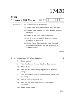


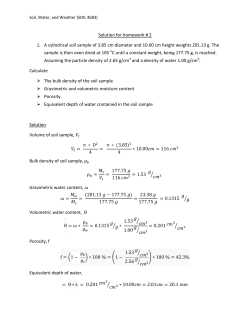


© Copyright 2026