1. science
2. social science
3. linguistics

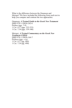
The lavaan tutorial
Yves Rosseel
Department of Data Analysis
Ghent University (Belgium)
January 15, 2015
Abstract
If you are new to lavaan, this is the place to start. In this tutorial, we introduce the basic components
of lavaan: the model syntax, the fitting functions (cfa, sem and growth), and the main extractor functions
(summary, coef, fitted, inspect). After we have provided two simple examples, we briefly discuss some important topics: meanstructures, multiple groups, growth curve models, mediation analysis, and categorical
data. Along the way, we hope to give you just enough information to get you started (but no more).
Contents
1 Before you start
1
2 Installation of the package
2
3 The model syntax
2
4 A first example: confirmatory factor analysis (CFA)
4
5 A second example: a structural equation model (SEM)
8
6 More about the syntax
11
7 Bringing in the means
14
8 Multiple groups
16
9 Growth curve models
25
10 Using categorical variables
28
11 Using a covariance matrix as input
28
12 Estimators, standard errors and missing values
30
13 Indirect effects and mediation analysis
31
14 Modification Indices
32
15 Extracting information from a fitted model
33
1
Before you start
Before you start, please read these points carefully:
• First of all, you must have a recent version (3.0.0 or higher) of R installed. You can download the latest
version of R from this page: http://cran.r-project.org/.
• The lavaan package is not finished yet. But it is already very useful for most users, or so we hope.
However, some important features that are currently NOT available in lavaan are:
1
– support for hierarchical/multilevel datasets (multilevel cfa, multilevel sem)
– support for discrete latent variables (mixture models, latent classes)
– Bayesian estimation
We hope to add these features in the next (two?) year(s) or so.
• We consider the current version as beta software. This does NOT mean that you can not trust the
results. We believe the results are accurate. It does mean that things may change when new versions
come out. For example, we may change the name of the arguments in function calls. And we change the
internals of the source code constantly. However, the model syntax is fairly mature and has been stable
for a while.
• We do not expect you to be an expert in R. In fact, the lavaan package is designed to be used by users
that would normally never use R. Nevertheless, it may help to familiarize yourself a bit with R, just to
be comfortable with it. Perhaps the most important skill that you may need to learn is how to import
your own datasets (perhaps in an SPSS format) into R. There are many tutorials on the web to teach
you just that. Once you have your data in R, you can start specifying your model. We have tried very
hard to make it as easy as possible for users to fit their models. Of course, if you have suggestions on
how we can improve things, please let us know.
• This document is written for first-time users of the lavaan package. It is not a reference manual, nor
does it contain technical material on how things are done in the lavaan package. These documents are
currently under preparation.
• The lavaan package is free open-source software. This means (among other things) that there is no
warranty whatsoever.
• If you need help, you can ask questions in the lavaan discussion group. Go to https://groups.google.
com/d/forum/lavaan/ and join the group. Once you have joined the group, you can email your questions to [email protected]. If you think you have found a bug, or if you have a suggestion for
improvement, you can either email me directly (to alert me), post it to the discussion group (to discuss
it), or open an issue on github (see https://github.com/yrosseel/lavaan/issues). The latter is
useful once we have agreed it is a bug, and it should be fixed. If you report a bug, it is always very useful
to provide a reproducible example (a short R script and some data).
2
Installation of the package
Since May 2010, the lavaan package is available on CRAN. Therefore, to install lavaan, simply start up R, and
type:
install.packages("lavaan", dependencies = TRUE)
You can check if the installation was succesful by typing
library(lavaan)
When the package is loaded, a startup message will be displayed showing the version number, and a reminder
that this is beta software:
This is lavaan 0.5-13
lavaan is BETA software! Please report any bugs.
If you see this message, you are ready to start.
3
The model syntax
At the heart of the lavaan package is the ‘model syntax’. The model syntax is a description of the model to be
estimated. In this section, we briefly explain the elements of the lavaan model syntax. More details are given
in the examples that follow.
In the R environment, a regression formula has the following form:
2
y ~ x1 + x2 + x3 + x4
In this formula, the tilde (“~”) is the regression operator. On the left-hand side of the operator, we have the
dependent variable (y), and on the right-hand side, we have the independent variables, separated by the “+”
operator. In lavaan, a typical model is simply a set (or system) of regression formulas, where some variables
(starting with an ‘f’ below) may be latent. For example:
y ~ f1 + f2 + x1 + x2
f1 ~ f2 + f3
f2 ~ f3 + x1 + x2
If we have latent variables in any of the regression formulas, we must ‘define’ them by listing their (manifest
or latent) indicators. We do this by using the special operator “=~”, which can be read as is measured by. For
example, to define the three latent variabels f1, f2 and f3, we can use something like:
f1 =~ y1 + y2 + y3
f2 =~ y4 + y5 + y6
f3 =~ y7 + y8 + y9 + y10
Furthermore, variances and covariances are specified using a ‘double tilde’ operator, for example:
y1 ~~ y1
y1 ~~ y2
f1 ~~ f2
# variance
# covariance
# covariance
And finally, intercepts for observed and latent variables are simple regression formulas with only an intercept
(explicitly denoted by the number ‘1’) as the only predictor:
y1 ~ 1
f1 ~ 1
Using these four formula types, a large variety of latent variable models can be described. The current set of
formula types is summarized in the table below.
formula type
operator
mnemonic
latent variable definition
=~
is measured by
regression
~
is regressed on
(residual) (co)variance
~~
is correlated with
intercept
~ 1
intercept
A complete lavaan model syntax is simply a combination of these formula types, enclosed between single
quotes. For example:
myModel <- ’ # regressions
y1 + y2 ~ f1 + f2 + x1 + x2
f1 ~ f2 + f3
f2 ~ f3 + x1 + x2
# latent variable
f1 =~ y1 + y2 +
f2 =~ y4 + y5 +
f3 =~ y7 + y8 +
definitions
y3
y6
y9 + y10
# variances and covariances
y1 ~~ y1
y1 ~~ y2
f1 ~~ f2
3
# intercepts
y1 ~ 1
f1 ~ 1
’
You can type this syntax interactively at the R prompt, but it is much more convenient to type the whole
model syntax first in an external text editor. And when you are done, you can copy/paste it to the R console.
If you are using RStudio, open a new ‘R script’, and type your model syntax (and all other R commands
needed for this session) in the source editor of RStudio. And save your script, so you can reuse it later on.
The code piece above will produce a model syntax object, called myModel that can be used later when calling
a function that actually estimates this model given a dataset. Note that formulas can be split over multiple
lines, and you can use comments (starting with the # character) and blank lines within the single quotes to
improve the readability of the model syntax.
If your model syntax is rather long, or you need to reuse the model syntax over and over again, you may prefer
to store it in a separate text file called, say, myModel.lav. This text file should be in a human readable format
(not a Word document). Within R, you can then read the model syntax from the file as follows:
myModel <- readLines("/mydirectory/myModel.lav")
The argument of readLines is the full path to the file containing the model syntax. Again, the model syntax
object can be used later to fit this model given a dataset.
4
A first example: confirmatory factor analysis (CFA)
We start with a simple example of confirmatory factor analysis, using the cfa() function, which is a userfriendly function for fitting CFA models. The lavaan package contains a built-in dataset called HolzingerSwineford1939.
See the help page for this dataset by typing
?HolzingerSwineford1939
at the R prompt. This is a ‘classic’ dataset that is used in many papers and books on Structural Equation
Modeling (SEM), including some manuals of commercial SEM software packages. The data consists of mental
ability test scores of seventh- and eighth-grade children from two different schools (Pasteur and Grant-White).
In our version of the dataset, only 9 out of the original 26 tests are included. A CFA model that is often
proposed for these 9 variables consists of three latent variables (or factors), each with three indicators:
• a visual factor measured by 3 variables: x1, x2 and x3
• a textual factor measured by 3 variables: x4, x5 and x6
• a speed factor measured by 3 variables: x7, x8 and x9
The figure below contains a graphical representation of the three-factor model.
4
x1
x2
x3
visual
x4
x5
textual
x6
speed
x7
x8
x9
The corresponding lavaan syntax for specifying this model is as follows:
visual =~ x1 + x2 + x3
textual =~ x4 + x5 + x6
speed =~ x7 + x8 + x9
In this example, the model syntax only contains three ‘latent variable definitions’. Each formula has the
following format:
latent variable =~ indicator1 + indicator2 + indicator3
We call these expressions latent variable definitions because they define how the latent variables are ‘manifested
by’ a set of observed (or manifest) variables, often called ‘indicators’. Note that the special “=~" operator in
the middle consists of a sign (”=“) character and a tilde ("~") character next to each other. The reason why
this model syntax is so short, is that behind the scenes, the function will take care of several things. First,
by default, the factor loading of the first indicator of a latent variable is fixed to 1, thereby fixing the scale
of the latent variable. Second, residual variances are added automatically. And third, all exogenous latent
variables are correlated by default. This way, the model syntax can be kept concise. On the other hand, the
user remains in control, since all this ‘default’ behavior can be overriden and/or switched off.
We can enter the model syntax using the single quotes:
HS.model <- ’ visual =~ x1 + x2 + x3
textual =~ x4 + x5 + x6
speed
=~ x7 + x8 + x9 ’
We can now fit the model as follows:
5
fit <- cfa(HS.model, data = HolzingerSwineford1939)
The cfa() function is a dedicated function for fitting confirmatory factor analysis models. The first argument
is the user-specified model. The second argument is the dataset that contains the observed variables. Once
the model has been fitted, the summary() function provides a nice summary of the fitted model:
summary(fit, fit.measures = TRUE)
The output should look familiar to users of other SEM software. If you find it confusing or esthetically
unpleasing, please let us know, and we will try to improve it.
lavaan (0.5-13) converged normally after
41 iterations
Number of observations
301
Estimator
Minimum Function Test Statistic
Degrees of freedom
P-value (Chi-square)
ML
85.306
24
0.000
Model test baseline model:
Minimum Function Test Statistic
Degrees of freedom
P-value
918.852
36
0.000
Full model versus baseline model:
Comparative Fit Index (CFI)
Tucker-Lewis Index (TLI)
0.931
0.896
Loglikelihood and Information Criteria:
Loglikelihood user model (H0)
Loglikelihood unrestricted model (H1)
-3737.745
-3695.092
Number of free parameters
Akaike (AIC)
Bayesian (BIC)
Sample-size adjusted Bayesian (BIC)
21
7517.490
7595.339
7528.739
Root Mean Square Error of Approximation:
RMSEA
90 Percent Confidence Interval
P-value RMSEA <= 0.05
0.071
0.092
0.114
0.001
Standardized Root Mean Square Residual:
SRMR
0.065
Parameter estimates:
Information
Standard Errors
Expected
Standard
Estimate
Latent variables:
visual =~
x1
Std.err
Z-value
P(>|z|)
1.000
6
x2
x3
textual =~
x4
x5
x6
speed =~
x7
x8
x9
Covariances:
visual ~~
textual
speed
textual ~~
speed
Variances:
x1
x2
x3
x4
x5
x6
x7
x8
x9
visual
textual
speed
0.553
0.729
0.100
0.109
5.554
6.685
0.000
0.000
1.000
1.113
0.926
0.065
0.055
17.014
16.703
0.000
0.000
1.000
1.180
1.082
0.165
0.151
7.152
7.155
0.000
0.000
0.408
0.262
0.074
0.056
5.552
4.660
0.000
0.000
0.173
0.049
3.518
0.000
0.549
1.134
0.844
0.371
0.446
0.356
0.799
0.488
0.566
0.809
0.979
0.384
0.114
0.102
0.091
0.048
0.058
0.043
0.081
0.074
0.071
0.145
0.112
0.086
The output consists of three parts. The first six lines are called the header. The header contains the following
information:
•
•
•
•
•
the
did
the
the
the
lavaan version number
lavaan converge normally or not, and how many iterations were needed
number of observations that were effectively used in the analysis
estimator that was used to obtain the parameter values (here: ML)
model test statistic, the degrees of freedom, and a corresponding p-value
The next section contains additional fit measures, and is only shown because we use the optional argument
fit.measures = TRUE. It starts with the line Model test baseline model and ends with the value for the
SRMR. The last section contains the parameter estimates. It starts with information about the standard errors (if
the information matrix is expected or observed, and if the standard errors are standard, robust, or based on the
bootstrap). Then, it tabulates all free (and fixed) parameters that were included in the model. Typically, first
the latent variables are shown, followed by covariances and (residual) variances. The first column (Estimate)
contains the (estimated or fixed) parameter value for each model parameter; the second column (Std.err)
contains the standard error for each estimated parameter; the third column (Z-value) contains the Wald
statistic (which is simply obtained by dividing the parameter value by its standard error), and the last column
(P(>|z|)) contains the p-value for testing the null hypothesis that the parameter equals zero in the population.
To wrap up this first example, we summarize the complete code that was needed to fit this three-factor model:
# load the lavaan package (only needed once per session)
library(lavaan)
# specify the model
HS.model <- ’ visual =~ x1 + x2 + x3
textual =~ x4 + x5 + x6
speed
=~ x7 + x8 + x9 ’
7
# fit the model
fit <- cfa(HS.model, data=HolzingerSwineford1939)
# display summary output
summary(fit, fit.measures=TRUE)
Simply copying this code and pasting it in R should work. The syntax illustrates the typical workflow in the
lavaan package:
1. Specify your model using the lavaan model syntax. In this example, only latent variable definitions have
been used. In the following examples, other formula types will be used.
2. Fit the model. This requires a dataset containing the observed variables (or alternatively the sample
covariance matrix and the number of observations). In this example, we have used the cfa() function.
Other funcions in the lavaan package are sem() and growth() for fitting full structural equation models
and growth curve models respectively. All three functions are so-called user-friendly functions, in the
sense that they take care of many details automatically, so we can keep the model syntax simple and
concise. If you wish to fit non-standard models or if you don’t like the idea that things are done for you
automatically, you can use the lower-level function lavaan() instead, where you have full control.
3. Extract information from the fitted model. This can be a long verbose summary, or it can be a single
number only (say, the RMSEA value). In the spirit of R, you only get what you asked for. We try to
not print out unnecessary information that you would ignore anyway.
5
A second example: a structural equation model (SEM)
In our second example, we will use the built-in PoliticalDemocracy dataset. This is a dataset that has been
used by Bollen in his 1989 book on structural equation modeling (and elsewhere). To learn more about the
dataset, see its help page and the references therein.
The figure below contains a graphical representation of the model that we want to fit.
The corresponding lavaan syntax for specifying this model is as follows:
model <- ’
# measurement model
ind60 =~ x1 + x2 + x3
dem60 =~ y1 + y2 + y3 + y4
dem65 =~ y5 + y6 + y7 + y8
# regressions
dem60 ~ ind60
dem65 ~ ind60 + dem60
# residual correlations
y1 ~~ y5
y2 ~~ y4 + y6
y3 ~~ y7
y4 ~~ y8
y6 ~~ y8
’
In this example, we use three different formula types: latent variabele definitions (using the =~ operator),
regression formulas (using the ~ operator), and (co)variance formulas (using the ~~ operator). The regression
formulas are similar to ordinary formulas in R. The (co)variance formulas typically have the following form:
variable ~~ variable
The variables can be either observed or latent variables. If the two variable names are the same, the expression
refers to the variance (or residual variance) of that variable. If the two variable names are different, the
expression refers to the (residual) covariance among these two variables. The lavaan package automatically
makes the distinction between variances and residual variances.
In our example, the expression y1 ~~ y5 allows the residual variances of the two observed variables to be
correlated. This is sometimes done if it is believed that the two variables have something in common that is
8
not captured by the latent variables. In this case, the two variables refer to identical scores, but measured in
two different years (1960 and 1965, respectively). Note that the two expressions y2 ~~ y4 and y2 ~~ y6, can
be combined into the expression y2 ~~ y4 + y6. This is just a shorthand notation.
We enter the model syntax as follows:
model <- ’
# measurement model
ind60 =~ x1 + x2 + x3
dem60 =~ y1 + y2 + y3 + y4
dem65 =~ y5 + y6 + y7 + y8
# regressions
dem60 ~ ind60
dem65 ~ ind60 + dem60
# residual correlations
y1 ~~ y5
y2 ~~ y4 + y6
y3 ~~ y7
y4 ~~ y8
y6 ~~ y8
’
To fit the model and see the results we can type:
fit <- sem(model, data = PoliticalDemocracy)
summary(fit, standardized = TRUE)
lavaan (0.5-13) converged normally after
68 iterations
Number of observations
75
Estimator
Minimum Function Test Statistic
Degrees of freedom
P-value (Chi-square)
ML
38.125
35
0.329
Parameter estimates:
Information
Standard Errors
Latent variables:
ind60 =~
x1
x2
x3
dem60 =~
y1
y2
y3
y4
dem65 =~
y5
y6
y7
y8
Regressions:
dem60 ~
ind60
Expected
Standard
Estimate
Std.err
Z-value
P(>|z|)
Std.lv
Std.all
1.000
2.180
1.819
0.139
0.152
15.742
11.967
0.000
0.000
0.670
1.460
1.218
0.920
0.973
0.872
1.000
1.257
1.058
1.265
0.182
0.151
0.145
6.889
6.987
8.722
0.000
0.000
0.000
2.223
2.794
2.351
2.812
0.850
0.717
0.722
0.846
1.000
1.186
1.280
1.266
0.169
0.160
0.158
7.024
8.002
8.007
0.000
0.000
0.000
2.103
2.493
2.691
2.662
0.808
0.746
0.824
0.828
1.483
0.399
3.715
0.000
0.447
0.447
9
dem65 ~
ind60
dem60
Covariances:
y1 ~~
y5
y2 ~~
y4
y6
y3 ~~
y7
y4 ~~
y8
y6 ~~
y8
Variances:
x1
x2
x3
y1
y2
y3
y4
y5
y6
y7
y8
ind60
dem60
dem65
0.572
0.837
0.221
0.098
2.586
8.514
0.010
0.000
0.182
0.885
0.182
0.885
0.624
0.358
1.741
0.082
0.624
0.296
1.313
2.153
0.702
0.734
1.871
2.934
0.061
0.003
1.313
2.153
0.273
0.356
0.795
0.608
1.308
0.191
0.795
0.191
0.348
0.442
0.787
0.431
0.348
0.109
1.356
0.568
2.386
0.017
1.356
0.338
0.082
0.120
0.467
1.891
7.373
5.067
3.148
2.351
4.954
3.431
3.254
0.448
3.956
0.172
0.019
0.070
0.090
0.444
1.374
0.952
0.739
0.480
0.914
0.713
0.695
0.087
0.921
0.215
0.082
0.120
0.467
1.891
7.373
5.067
3.148
2.351
4.954
3.431
3.254
1.000
0.800
0.039
0.154
0.053
0.239
0.277
0.486
0.478
0.285
0.347
0.443
0.322
0.315
1.000
0.800
0.039
The function sem() is very similar to the function cfa(). In fact, the two functions are currently almost
identical, but this may change in the future. In the summary() function, we omitted the fit.measures=TRUE
argument. Therefore, you only get the basic chi-square test statistic. The argument standardized=TRUE
augments the output with standardized parameter values. Two extra columns of standardized parameter
values are printed. In the first column (labeled Std.lv), only the latent variables are standardized. In the
second column (labeled Std.all), both latent and observed variables are standardized. The latter is often
called the ‘completely standardized solution’.
The complete code to specify and fit this model is printed again below:
library(lavaan) # only needed once per session
model <- ’
# measurement model
ind60 =~ x1 + x2 + x3
dem60 =~ y1 + y2 + y3 + y4
dem65 =~ y5 + y6 + y7 + y8
# regressions
dem60 ~ ind60
dem65 ~ ind60 + dem60
# residual correlations
y1 ~~ y5
y2 ~~ y4 + y6
y3 ~~ y7
y4 ~~ y8
y6 ~~ y8
’
fit <- sem(model, data=PoliticalDemocracy)
summary(fit, standardized=TRUE)
10
6
More about the syntax
Fixing parameters Consider a simple one-factor model with 4 indicators. By default, lavaan will always
fix the factor loading of the first indicator to 1. The other three factor loadings are free, and their values are
estimated by the model. But suppose that you have good reasons the fix all the factor loadings to 1. The
syntax below illustrates how this can be done:
f =~ y1 + 1*y2 + 1*y3 + 1*y4
In general, to fix a parameter in a lavaan formula, you need to pre-multiply the corresponding variable in
the formula by a numerical value. This is called the pre-multiplication mechanism and will be used for many
purposes. As another example, consider again the three-factor Holzinger and Swineford CFA model. Recall
that, by default, all exogenous latent variables in a CFA model are correlated. But if you wish to fix the
correlation (or covariance) between a pair of latent variables to zero, you need to explicity add a covarianceformula for this pair, and fix the parameter to zero. In the syntax below, we allow the covariance between the
latent variables visual and textual to be free, but the two other covariances are fixed to zero. In addition,
we fix the variance of the factor speed to unity. Therefore, there is no need anymore to set the factor loading
of its first indicator (x7) equal to one. To force this factor loading to be free, we pre-multiply it with NA, as a
hint to lavaan that the value of this parameter is still unknown.
# three-factor model
visual =~ x1 + x2 + x3
textual =~ x4 + x5 + x6
speed
=~ NA*x7 + x8 + x9
# orthogonal factors
visual ~~ 0*speed
textual ~~ 0*speed
# fix variance of speed factor
speed ~~ 1*speed
If you need to constrain all covariances of the latent variables in a CFA model to be orthogonal, there is a shortcut. You can omit the covariance formulas in the model syntax and simply add an argument orthogonal=TRUE
to the function call:
HS.model <- ’
visual =~ x1 + x2 + x3
textual =~ x4 + x5 + x6
speed
=~ x7 + x8 + x9 ’
fit.HS.ortho <- cfa(HS.model,
data = HolzingerSwineford1939,
orthogonal = TRUE)
Similarly, if you want to fix the variances of all the latent variables in a CFA model to unity, there is again a
shortcut. Simply add the argument std.lv=TRUE to the function call:
HS.model <- ’ visual =~ x1 + x2 + x3
textual =~ x4 + x5 + x6
speed
=~ x7 + x8 + x9 ’
fit <- cfa(HS.model,
data = HolzingerSwineford1939,
std.lv = TRUE)
If the argument std.lv=TRUE is used, the factor loadings of the first indicator of each latent variable will no
longer be fixed to 1.
Starting Values The lavaan package automatically generates starting values for all free parameters. Normally, this works fine. But if you must provide your own starting values, you are free to do so. The way it
works is based on the pre-multiplication mechanism that we discussed before. But the numeric constant is
now the argument of a special function start(). An example will make this clear:
visual =~ x1 + start(0.8)*x2 + start(1.2)*x3
textual =~ x4 + start(0.5)*x5 + start(1.0)*x6
speed
=~ x7 + start(0.7)*x8 + start(1.8)*x9
11
Parameter labels A nice property of the lavaan package is that all free parameters are automatically named
according to a simple set of rules. This is convenient, for example, if equality constraints are needed (see the
next subsection). To see how the naming mechanism works, we will use the model that we used for the Politcal
Democracy data.
model <- ’
# latent variable definitions
ind60 =~ x1 + x2 + x3
dem60 =~ y1 + y2 + y3 + y4
dem65 =~ y5 + y6 + y7 + y8
# regressions
dem60 ~ ind60
dem65 ~ ind60 + dem60
# residual (co)variances
y1 ~~ y5
y2 ~~ y4 + y6
y3 ~~ y7
y4 ~~ y8
y6 ~~ y8
’
fit <- sem(model,
data = PoliticalDemocracy)
coef(fit)
ind60=~x2
2.180
dem65=~y6
1.186
dem65~dem60
0.837
y4~~y8
0.348
y1~~y1
1.891
y6~~y6
4.954
dem65~~dem65
0.172
ind60=~x3
1.819
dem65=~y7
1.280
y1~~y5
0.624
y6~~y8
1.356
y2~~y2
7.373
y7~~y7
3.431
dem60=~y2
dem60=~y3
dem60=~y4
1.257
1.058
1.265
dem65=~y8 dem60~ind60 dem65~ind60
1.266
1.483
0.572
y2~~y4
y2~~y6
y3~~y7
1.313
2.153
0.795
x1~~x1
x2~~x2
x3~~x3
0.082
0.120
0.467
y3~~y3
y4~~y4
y5~~y5
5.067
3.148
2.351
y8~~y8 ind60~~ind60 dem60~~dem60
3.254
0.448
3.956
The function coef() extracts the estimated values of the free parameters in the model, together with their
names. Each name consists of three parts and reflects the part of the formula where the parameter was
involved. The first part is the variable name that appears on the left-hand side of the formula. The middle
part is the operator type of the formula, and the third part is the variable in the right-hand side of the formula
that corresponds with the parameter.
Often, it is convenient to choose your own labels for specific parameters. The way this works is similar to
fixing a parameter. But instead of pre-multiplying with a numerical constant, we use a character string (the
label) instead. In the example below, we ‘label’ the factor loading of the x3 indicator with the label myLabel:
model <- ’
# latent variable definitions
ind60 =~ x1 + x2 + myLabel*x3
dem60 =~ y1 + y2 + y3 + y4
dem65 =~ y5 + y6 + y7 + y8
# regressions
dem60 ~ ind60
dem65 ~ ind60 + dem60
# residual (co)variances
y1 ~~ y5
y2 ~~ y4 + y6
y3 ~~ y7
12
y4 ~~ y8
y6 ~~ y8
’
It is important that labels start with a letter (a-zA-Z), and certainly not with a digit. For example ‘13bis’
is not a valid label, and will confuse the lavaan syntax parser. Note: before version 0.4-8, it was necessary
to use the modifier label() to specify a custom label. Although it is still supported, it is not recommended
anymore. The only reason why it should be used in new syntax is if the label contains an operator like “~” or
“=~”.
Modifiers We have seen the use of the pre-multiplication mechanism (using the * operator) a number of
times: to fix a parameter, to provide a starting value, and to label a parameter. We refer to these operations as
modifiers, because they modify some properties of certain model parameters. More modifiers will be introduced
later.
Each term on the right hand side in a formula can have one modifier only. If you must specify more modifiers
for the same parameter, you need to list the term multiple times in the same formula. For example:
f =~ y1 + y2 + myLabel*y3 + start(0.5)*y3 + y4
The indicator y3 was listed twice, each time with a different modifier. The parser will accumulate all the
different modifiers, but still treat y3 as a single indicator.
Simple equality constraints In some applications, it is useful to impose equality constraints on one or
more otherwise free parameters. Consider again the three-factor H&S CFA model. Suppose a user has a priori
reasons to believe that the factor loadings of the x2 and x3 indicators are equal to each other. Instead of
estimating two free parameters, lavaan should only estimate a single free parameter, and use that value for
both factor loadings. The main mechanism to specify this type of (simple) equality constraints is by using
labels: if two parameters have the same label, they will be considered to be the same, and only one value will
be computed for them. This is illustrated in the following syntax:
visual =~ x1 + v2*x2 + v2*x3
textual =~ x4 + x5 + x6
speed
=~ x7 + x8 + x9
Remember: all parameters having the same label will be constrained to be equal.
An alternative approach is to use the equal() modifier. This is useful if no custom label has been specified,
and one needs to refer to the automatically generated label. For example:
visual =~ x1 + x2 + equal("visual=~x2")*x3
textual =~ x4 + x5 + x6
speed
=~ x7 + x8 + x9
Nonlinear equality and inequality constraints
Consider the following regression:
y ~ b1*x1 + b2*x2 + b3*x3
where we have explicitly labeled the regression coefficients as b1, b2 and b3. We create a toy dataset containing
these four variables and fit the regression model:
set.seed(1234)
Data <- data.frame(y = rnorm(100),
x1 = rnorm(100),
x2 = rnorm(100),
x3 = rnorm(100))
model <- ’ y ~ b1*x1 + b2*x2 + b3*x3 ’
fit <- sem(model, data=Data)
coef(fit)
b1
-0.052
b2
0.084
b3
0.139
y~~y
0.970
13
Suppose that we need to impose the following two (nonlinear) constraints on b1 : b1 = (b2 + b3 )2 and b1 ≥
exp(b2 + b3 ). The first constraint is an equality constraint. The second is an inequality constraint. To specify
these constraints, you can use the following syntax:
model.constr <- ’ # model with labeled parameters
y ~ b1*x1 + b2*x2 + b3*x3
# constraints
b1 == (b2 + b3)^2
b1 > exp(b2 + b3) ’
To see the effect of the constraints, we refit the model:
model.constr <- ’ # model with labeled parameters
y ~ b1*x1 + b2*x2 + b3*x3
# constraints
b1 == (b2 + b3)^2
b1 > exp(b2 + b3) ’
fit <- sem(model.constr, data=Data)
coef(fit)
b1
b2
b3
0.495 -0.405 -0.299
y~~y
1.610
The reader can verify that the constraints are indeed respected. The equality constraint holds exactly. The
inequality constraint has resulted in an equality between the left-hand side (b1 ) and the right-hand side
(exp(b2 + b3 )).
7
Bringing in the means
By and large, structural equation models are used to model the covariance matrix of the observed variables in
a dataset. But in some applications, it is useful to bring in the means of the observed variables too. One way
to do this is to explicitly refer to intercepts in the lavaan syntax. This can be done by including ‘intercept
formulas’ in the model syntax. An intercept formula has the following form:
variable ~ 1
The left part of the expression contains the name of the observed or latent variable. The right part contains
the number 1, representing the intercept. For example, in the three-factor H&S CFA model, we can add the
intercepts of the observed variables as follows:
# three-factor model
visual =~ x1 + x2 + x3
textual =~ x4 + x5 + x6
speed
=~ x7 + x8 + x9
# intercepts
x1 ~ 1
x2 ~ 1
x3 ~ 1
x4 ~ 1
x5 ~ 1
x6 ~ 1
x7 ~ 1
x8 ~ 1
x9 ~ 1
However, it is more convenient to omit the intercept formulas in the model syntax (unless you want to fix their
values), and to add the argument meanstructure = TRUE in the fitting function. For example, we can refit
the three-factor H&S CFA model as follows:
14
fit <- cfa(HS.model,
data = HolzingerSwineford1939,
meanstructure = TRUE)
summary(fit)
lavaan (0.5-13) converged normally after
41 iterations
Number of observations
301
Estimator
Minimum Function Test Statistic
Degrees of freedom
P-value (Chi-square)
ML
85.306
24
0.000
Parameter estimates:
Information
Standard Errors
Expected
Standard
Estimate
Std.err
Z-value
P(>|z|)
1.000
0.553
0.729
0.100
0.109
5.554
6.685
0.000
0.000
1.000
1.113
0.926
0.065
0.055
17.014
16.703
0.000
0.000
1.000
1.180
1.082
0.165
0.151
7.152
7.155
0.000
0.000
0.408
0.262
0.074
0.056
5.552
4.660
0.000
0.000
0.173
0.049
3.518
0.000
Intercepts:
x1
x2
x3
x4
x5
x6
x7
x8
x9
visual
textual
speed
4.936
6.088
2.250
3.061
4.341
2.186
4.186
5.527
5.374
0.000
0.000
0.000
0.067
0.068
0.065
0.067
0.074
0.063
0.063
0.058
0.058
73.473
89.855
34.579
45.694
58.452
34.667
66.766
94.854
92.546
0.000
0.000
0.000
0.000
0.000
0.000
0.000
0.000
0.000
Variances:
x1
x2
x3
0.549
1.134
0.844
0.114
0.102
0.091
Latent variables:
visual =~
x1
x2
x3
textual =~
x4
x5
x6
speed =~
x7
x8
x9
Covariances:
visual ~~
textual
speed
textual ~~
speed
15
x4
x5
x6
x7
x8
x9
visual
textual
speed
0.371
0.446
0.356
0.799
0.488
0.566
0.809
0.979
0.384
0.048
0.058
0.043
0.081
0.074
0.071
0.145
0.112
0.086
As you can see in the output, the model includes intercept parameters for both the observed and latent
variables. By default, the cfa() and sem() functions fix the latent variable intercepts (which in this case
correspond to the latent means) to zero. Otherwise, the model would not be estimable. Note that the chisquare statistic and the number of degrees of freedom is the same as in the original model (without a mean
structure). The reason is that we brought in some new data (a mean value for each of the 9 observed variables),
but we also added 9 additional parameters to the model (an intercept for each of the 9 observed variables).
The end result is an identical fit. In practice, the only reason why a user would add intercept-formulas in the
model syntax, is because some constraints must be specified on them. For example, suppose that we wish to
fix the intercepts of the variables x1, x2, x3 and x4 to, say, 0.5. We would write the model syntax as follows:
# three-factor model
visual =~ x1 + x2 + x3
textual =~ x4 + x5 + x6
speed
=~ x7 + x8 + x9
# intercepts with fixed values
x1 + x2 + x3 + x4 ~ 0.5*1
where we have used the left-hand side of the formula to ‘repeat’ the right-hand side for each element of the
left-hand side.
8
Multiple groups
The lavaan package has full support for multiple groups. To request a multiple group analysis, you need to
add the name of the group variable in your dataset to the argument group in the fitting function. By default,
the same model is fitted in all groups. In the following example, we fit the H&S CFA model for the two schools
(Pasteur and Grant-White).
HS.model <- ’
visual =~ x1 + x2 + x3
textual =~ x4 + x5 + x6
speed
=~ x7 + x8 + x9 ’
fit <- cfa(HS.model,
data = HolzingerSwineford1939,
group = "school")
summary(fit)
lavaan (0.5-17.693) converged normally after
57 iterations
Number of observations per group
Pasteur
Grant-White
156
145
Estimator
Minimum Function Test Statistic
Degrees of freedom
P-value (Chi-square)
ML
115.851
48
0.000
Chi-square for each group:
Pasteur
Grant-White
64.309
51.542
16
Parameter estimates:
Information
Standard Errors
Expected
Standard
Group 1 [Pasteur]:
Estimate
Std.err
Z-value
P(>|z|)
1.000
0.394
0.570
0.122
0.140
3.220
4.076
0.001
0.000
1.000
1.183
0.875
0.102
0.077
11.613
11.421
0.000
0.000
1.000
1.125
0.922
0.277
0.225
4.057
4.104
0.000
0.000
0.479
0.185
0.106
0.077
4.531
2.397
0.000
0.017
0.182
0.069
2.628
0.009
Intercepts:
x1
x2
x3
x4
x5
x6
x7
x8
x9
visual
textual
speed
4.941
5.984
2.487
2.823
3.995
1.922
4.432
5.563
5.418
0.000
0.000
0.000
0.095
0.098
0.093
0.092
0.105
0.079
0.087
0.078
0.079
52.249
60.949
26.778
30.689
38.183
24.321
51.181
71.214
68.440
0.000
0.000
0.000
0.000
0.000
0.000
0.000
0.000
0.000
Variances:
x1
x2
x3
x4
x5
x6
x7
x8
x9
visual
textual
speed
0.298
1.334
0.989
0.425
0.456
0.290
0.820
0.510
0.680
1.097
0.894
0.350
0.232
0.158
0.136
0.069
0.086
0.050
0.125
0.116
0.104
0.276
0.150
0.126
Latent variables:
visual =~
x1
x2
x3
textual =~
x4
x5
x6
speed =~
x7
x8
x9
Covariances:
visual ~~
textual
speed
textual ~~
speed
17
Group 2 [Grant-White]:
Estimate
Std.err
Z-value
P(>|z|)
1.000
0.736
0.925
0.155
0.166
4.760
5.583
0.000
0.000
1.000
0.990
0.963
0.087
0.085
11.418
11.377
0.000
0.000
1.000
1.226
1.058
0.187
0.165
6.569
6.429
0.000
0.000
0.408
0.276
0.098
0.076
4.153
3.639
0.000
0.000
0.222
0.073
3.022
0.003
Intercepts:
x1
x2
x3
x4
x5
x6
x7
x8
x9
visual
textual
speed
4.930
6.200
1.996
3.317
4.712
2.469
3.921
5.488
5.327
0.000
0.000
0.000
0.095
0.092
0.086
0.093
0.096
0.094
0.086
0.087
0.085
51.696
67.416
23.195
35.625
48.986
26.277
45.819
63.174
62.571
0.000
0.000
0.000
0.000
0.000
0.000
0.000
0.000
0.000
Variances:
x1
x2
x3
x4
x5
x6
x7
x8
x9
visual
textual
speed
0.715
0.899
0.557
0.315
0.419
0.406
0.600
0.401
0.535
0.604
0.942
0.461
0.126
0.123
0.103
0.065
0.072
0.069
0.091
0.094
0.089
0.160
0.152
0.118
Latent variables:
visual =~
x1
x2
x3
textual =~
x4
x5
x6
speed =~
x7
x8
x9
Covariances:
visual ~~
textual
speed
textual ~~
speed
If you want to fix parameters, or provide starting values, you can use the same pre-multiplication techniques,
but the single argument is now replaced by a vector of arguments, one for each group. If you use a single
element instead of a vector, that element will be applied for all groups (note: this is NOT true for labels, since
this would imply equality constraints). For example:
HS.model <- ’
visual =~ x1 + 0.5*x2 + c(0.6, 0.8)*x3
textual =~ x4 + start(c(1.2, 0.6))*x5 + a*x6
speed
=~ x7 + x8 + x9 ’
18
In the definition of the latent factor visual, we have fixed the factor loading of the indicator x3 to the value
‘0.6’ in the first group, and to the value ‘0.8’ in the second group, while the factor loading of the indicator x2
is fixed to the value ‘0.5’ in both groups. In the definition of the textual factor, two different starting values
are provided for the x5 indicator; one for each group. In addition, we have labeled the factor loading of the x6
indicator as ‘a’, but this label is only given to the parameter of the first group. If you want to provide labels
to each of the two groups, you can write something like c(a1,a2)*x6. Be careful: if you write c(a,a)*x6,
both parameters (in the first and second group) will get the same label, and hence they will be treated as a
single parameter. To verify the effects of these modifiers, we refit the model:
fit <- cfa(HS.model,
data = HolzingerSwineford1939,
group = "school")
summary(fit)
lavaan (0.5-17.693) converged normally after
48 iterations
Number of observations per group
Pasteur
Grant-White
156
145
Estimator
Minimum Function Test Statistic
Degrees of freedom
P-value (Chi-square)
ML
118.976
52
0.000
Chi-square for each group:
Pasteur
Grant-White
64.901
54.075
Parameter estimates:
Information
Standard Errors
Expected
Standard
Group 1 [Pasteur]:
Estimate
Latent variables:
visual =~
x1
x2
x3
textual =~
x4
x5
x6
(a)
speed =~
x7
x8
x9
Covariances:
visual ~~
textual
speed
textual ~~
speed
Std.err
Z-value
P(>|z|)
1.000
1.185
0.876
0.102
0.077
11.598
11.409
0.000
0.000
1.000
1.129
0.931
0.279
0.227
4.055
4.103
0.000
0.000
0.460
0.182
0.103
0.076
4.479
2.408
0.000
0.016
0.181
0.069
2.625
0.009
1.000
0.500
0.600
Intercepts:
19
x1
x2
x3
x4
x5
x6
x7
x8
x9
visual
textual
speed
4.941
5.984
2.487
2.823
3.995
1.922
4.432
5.563
5.418
0.000
0.000
0.000
0.094
0.100
0.092
0.092
0.105
0.079
0.087
0.078
0.079
52.379
59.945
26.983
30.689
38.183
24.321
51.181
71.214
68.440
0.000
0.000
0.000
0.000
0.000
0.000
0.000
0.000
0.000
Variances:
x1
x2
x3
x4
x5
x6
x7
x8
x9
visual
textual
speed
0.388
1.304
0.965
0.427
0.454
0.289
0.824
0.510
0.677
1.001
0.892
0.346
0.129
0.155
0.120
0.069
0.086
0.050
0.124
0.116
0.105
0.172
0.150
0.125
Std.err
Z-value
P(>|z|)
1.000
0.990
0.963
0.087
0.085
11.425
11.374
0.000
0.000
1.000
1.228
1.081
0.188
0.168
6.539
6.417
0.000
0.000
0.454
0.315
0.099
0.079
4.585
4.004
0.000
0.000
0.222
0.073
3.049
0.002
4.930
6.200
1.996
3.317
4.712
2.469
0.097
0.089
0.086
0.093
0.096
0.094
50.688
69.616
23.223
35.625
48.986
26.277
0.000
0.000
0.000
0.000
0.000
0.000
Group 2 [Grant-White]:
Estimate
Latent variables:
visual =~
x1
x2
x3
textual =~
x4
x5
x6
speed =~
x7
x8
x9
Covariances:
visual ~~
textual
speed
textual ~~
speed
Intercepts:
x1
x2
x3
x4
x5
x6
1.000
0.500
0.800
20
x7
x8
x9
visual
textual
speed
3.921
5.488
5.327
0.000
0.000
0.000
0.086
0.087
0.085
Variances:
x1
x2
x3
x4
x5
x6
x7
x8
x9
visual
textual
speed
0.637
0.966
0.601
0.316
0.418
0.407
0.609
0.411
0.522
0.735
0.942
0.453
0.115
0.120
0.091
0.065
0.072
0.069
0.091
0.094
0.089
0.132
0.152
0.117
45.819
63.174
62.571
0.000
0.000
0.000
Fixing parameters in some groups, but not all Sometimes, we wish to fix the value of a parameter
in all groups, except for one particular group. In this group, we wish to freely estimate the value of that
parameter. The modifier for this parameter is again a vector containing the fixed values for this parameter
for each group, but we can use NA to force a parameter to be free in one (or more) group(s). Suppose for
example we have four groups. We define a latent variable (say f) with three indicators. We wish to fix the
factor loading of indicator item2 to 1.0 in all but the second group. We can write something like
f =~ item1 + c(1,NA,1,1)*item2 + item3
Constraining a single parameter to be equal across groups If you want to constrain one or more
parameters to be equal across groups, you need to give them the same label. For example, to constrain the
factor loading of the indicator x3 to be equal across (two) groups, you can write:
HS.model <- ’
visual =~ x1 + x2 + c(v3,v3)*x3
textual =~ x4 + x5 + x6
speed
=~ x7 + x8 + x9 ’
Again, identical labels imply identical parameters, both within and across groups.
Constraining groups of parameters to be equal across groups Although providing identical labels is
a very flexible method to specify equality constraints for a few parameters, there is a more convenient way to
impose equality constraints on a whole set of parameters (for example: all factor loadings, or all intercepts). We
call these type of constraints group equality constraints and they can be specified by the argument group.equal
in the fitting function. For example, to constrain (all) the factor loadings to be equal across groups, you can
proceed as follows:
HS.model <- ’
visual =~ x1 + x2 + x3
textual =~ x4 + x5 + x6
speed
=~ x7 + x8 + x9 ’
fit <- cfa(HS.model,
data = HolzingerSwineford1939,
group = "school",
group.equal = c("loadings"))
summary(fit)
lavaan (0.5-17.693) converged normally after
41 iterations
Number of observations per group
21
Pasteur
Grant-White
156
145
Estimator
Minimum Function Test Statistic
Degrees of freedom
P-value (Chi-square)
ML
124.044
54
0.000
Chi-square for each group:
Pasteur
Grant-White
68.825
55.219
Parameter estimates:
Information
Standard Errors
Expected
Standard
Group 1 [Pasteur]:
Estimate
Std.err
Z-value
P(>|z|)
1.000
0.599
0.784
0.100
0.108
5.979
7.267
0.000
0.000
1.000
1.083
0.912
0.067
0.058
16.049
15.785
0.000
0.000
1.000
1.201
1.038
0.155
0.136
7.738
7.629
0.000
0.000
0.416
0.169
0.097
0.064
4.271
2.643
0.000
0.008
0.176
0.061
2.882
0.004
Intercepts:
x1
x2
x3
x4
x5
x6
x7
x8
x9
visual
textual
speed
4.941
5.984
2.487
2.823
3.995
1.922
4.432
5.563
5.418
0.000
0.000
0.000
0.093
0.100
0.094
0.093
0.101
0.081
0.086
0.078
0.079
52.991
60.096
26.465
30.371
39.714
23.711
51.540
71.088
68.153
0.000
0.000
0.000
0.000
0.000
0.000
0.000
0.000
0.000
Variances:
x1
x2
x3
0.551
1.258
0.882
0.137
0.155
0.128
Latent variables:
visual =~
x1
x2
x3
textual =~
x4
x5
x6
speed =~
x7
x8
x9
Covariances:
visual ~~
textual
speed
textual ~~
speed
22
x4
x5
x6
x7
x8
x9
visual
textual
speed
0.434
0.508
0.266
0.849
0.515
0.658
0.805
0.913
0.305
0.070
0.082
0.050
0.114
0.095
0.096
0.171
0.137
0.078
Group 2 [Grant-White]:
Estimate
Std.err
Z-value
P(>|z|)
1.000
0.599
0.784
0.100
0.108
5.979
7.267
0.000
0.000
1.000
1.083
0.912
0.067
0.058
16.049
15.785
0.000
0.000
1.000
1.201
1.038
0.155
0.136
7.738
7.629
0.000
0.000
0.437
0.314
0.099
0.079
4.423
3.958
0.000
0.000
0.226
0.072
3.144
0.002
Intercepts:
x1
x2
x3
x4
x5
x6
x7
x8
x9
visual
textual
speed
4.930
6.200
1.996
3.317
4.712
2.469
3.921
5.488
5.327
0.000
0.000
0.000
0.097
0.091
0.085
0.092
0.100
0.091
0.086
0.087
0.085
50.763
68.379
23.455
35.950
47.173
27.248
45.555
63.257
62.786
0.000
0.000
0.000
0.000
0.000
0.000
0.000
0.000
0.000
Variances:
x1
x2
x3
x4
x5
x6
x7
x8
x9
0.645
0.933
0.605
0.329
0.384
0.437
0.599
0.406
0.532
0.127
0.121
0.096
0.062
0.073
0.067
0.090
0.089
0.086
Latent variables:
visual =~
x1
x2
x3
textual =~
x4
x5
x6
speed =~
x7
x8
x9
Covariances:
visual ~~
textual
speed
textual ~~
speed
23
visual
textual
speed
0.722
0.906
0.475
0.161
0.136
0.109
More ‘group equality constraints’ can be added. In addition to the factor loadings, the following keywords are
supported in the group.equal argument:
•
•
•
•
•
•
•
intercepts: the intercepts of the observed variables
means: the intercepts/means of the latent variables
residuals: the residual variances of the observed variables
residual.covariances: the residual covariances of the observed variables
lv.variances: the (residual) variances of the latent variables
lv.covariances: the (residual) covariances of the latent varibles
regressions: all regression coefficients in the model
If you omit the group.equal argument, all parameters are freely estimated in each group (but the model
structure is the same).
But what if you want to constrain a whole group of parameters (say all factor loadings and intercepts) across
groups, except for one or two parameters that need to stay free in all groups. For this scenario, you can use the
argument group.partial, containing the names of those parameters that need to remain free. For example:
fit <- cfa(HS.model,
data = HolzingerSwineford1939,
group = "school",
group.equal = c("loadings", "intercepts"),
group.partial = c("visual=~x2", "x7~1"))
Measurement Invariance If you are interested in testing the measurement invariance of a CFA model
across several groups, you can use the function measurementInvariance() which performs a number of multiple group analyses in a particular sequence, with increasingly more restrictions on the parameters. (Note: from
the 0.5 series onwards, the measurementInvariance() function has been moved to the semTools package.)
Each model is compared to the baseline model and the previous model using chi-square difference tests. In
addition, the difference in the fit measure is also shown. Although the current implementation of the function is still a bit primitive, it does illustrate how the various components of the lavaan package can be used
as building blocks for constructing higher level functions (such as the measurementInvariance() function),
something that is often very hard to accomplish with commercial software.
library(semTools)
measurementInvariance(HS.model, data = HolzingerSwineford1939, group = "school")
Measurement invariance tests:
Model 1: configural invariance:
chisq
df
pvalue
cfi
115.851
48.000
0.000
0.923
rmsea
bic
0.097 7706.822
Model 2: weak invariance (equal loadings):
chisq
df
pvalue
cfi
rmsea
bic
124.044
54.000
0.000
0.921
0.093 7680.771
[Model 1 versus model 2]
delta.chisq
delta.df delta.p.value
8.192
6.000
0.224
delta.cfi
0.002
Model 3: strong invariance (equal loadings + intercepts):
chisq
df
pvalue
cfi
rmsea
bic
164.103
60.000
0.000
0.882
0.107 7686.588
24
[Model 1 versus model 3]
delta.chisq
delta.df delta.p.value
48.251
12.000
0.000
delta.cfi
0.041
[Model 2 versus model 3]
delta.chisq
delta.df delta.p.value
40.059
6.000
0.000
delta.cfi
0.038
Model 4: equal loadings + intercepts + means:
chisq
df
pvalue
cfi
rmsea
bic
204.605
63.000
0.000
0.840
0.122 7709.969
[Model 1 versus model 4]
delta.chisq
delta.df delta.p.value
88.754
15.000
0.000
delta.cfi
0.083
[Model 3 versus model 4]
delta.chisq
delta.df delta.p.value
40.502
3.000
0.000
delta.cfi
0.042
By adding the group.partial argument, you can test for partial measurement invariance by allowing a few
parameters to remain free.
9
Growth curve models
Another important type of latent variable models are latent growth curve models. Growth modeling is often
used to analyze longitudinal or developmental data. In this type of data, an outcome measure is measured on
several occasions, and we want to study the change over time. In many cases, the trajectory over time can be
modeled as a simple linear or quadratic curve. Random effects are used to capture individual differences. The
random effects are conveniently represented by (continuous) latent variables, often called growth factors. In
the example below, we use an artifical dataset called Demo.growth where a score (say, a standardized score on
a reading ability scale) is measured on 4 time points. To fit a linear growth model for these four time points,
we need to specify a model with two latent variables: a random intercept, and a random slope:
# linear growth model with
# intercept and slope with
i =~ 1*t1 + 1*t2 + 1*t3 +
s =~ 0*t1 + 1*t2 + 2*t3 +
4 timepoints
fixed coefficients
1*t4
3*t4
In this model, we have fixed all the coefficients of the growth functions. To fit this model, the lavaan package
provides a special growth() function:
model <- ’ i =~ 1*t1 + 1*t2 + 1*t3 + 1*t4
s =~ 0*t1 + 1*t2 + 2*t3 + 3*t4 ’
fit <- growth(model, data=Demo.growth)
summary(fit)
lavaan (0.5-13) converged normally after
44 iterations
Number of observations
400
Estimator
Minimum Function Test Statistic
Degrees of freedom
P-value (Chi-square)
ML
8.069
5
0.152
Parameter estimates:
Information
Standard Errors
Expected
Standard
25
Estimate
Latent variables:
i =~
t1
t2
t3
t4
s =~
t1
t2
t3
t4
Std.err
Z-value
P(>|z|)
1.000
1.000
1.000
1.000
0.000
1.000
2.000
3.000
Covariances:
i ~~
s
0.618
0.071
8.686
0.000
Intercepts:
t1
t2
t3
t4
i
s
0.000
0.000
0.000
0.000
0.615
1.006
0.077
0.042
8.007
24.076
0.000
0.000
Variances:
t1
t2
t3
t4
i
s
0.595
0.676
0.635
0.508
1.932
0.587
0.086
0.061
0.072
0.124
0.173
0.052
Technically, the growth() function is almost identical to the sem() function. But a mean structure is automatically assumed, and the observed intercepts are fixed to zero by default, while the latent variable intercepts/means are freely estimated. A slightly more complex model adds two regressors (x1 and x2) that
influence the latent growth factors. In addition, a time-varying covariate c that influences the outcome measure
at the four time points has been added to the model. A graphical representation of this model is presented
below.
26
t1
c1
t2
c2
t3
t4
c3
c4
i
s
x1
x2
The corresponding syntax is the following:
# intercept and slope
# with fixed coefficients
i =~ 1*t1 + 1*t2 + 1*t3 + 1*t4
s =~ 0*t1 + 1*t2 + 2*t3 + 3*t4
# regressions
i ~ x1 + x2
s ~ x1 + x2
# time-varying covariates
t1 ~ c1
t2 ~ c2
t3 ~ c3
t4 ~ c4
For ease of copy/pasting, the complete R code needed to specify and fit this linear growth model with a
time-varying covariate is printed again below:
# a linear growth model with a time-varying covariate
model <- ’
# intercept and slope with fixed coefficients
i =~ 1*t1 + 1*t2 + 1*t3 + 1*t4
s =~ 0*t1 + 1*t2 + 2*t3 + 3*t4
# regressions
i ~ x1 + x2
s ~ x1 + x2
# time-varying covariates
t1 ~ c1
27
t2 ~ c2
t3 ~ c3
t4 ~ c4
’
fit <- growth(model, data = Demo.growth)
summary(fit)
10
Using categorical variables
Binary, ordinal and nominal variables are considered categorical (not continuous). It makes a big difference if
these categorical variables are exogenous (independent) or endogenous (dependent) in the model.
Exogenous categorical variables If you have a binary exogenous covariate (say, gender), all you need to
do is to recode it as a dummy (0/1) variable. Just like you would do in a classic regression model. If you have
an exogenous ordinal variable, you can use a coding scheme reflecting the order (say, 1,2,3,. . . ) and treat it
as any other (numeric) covariate. If you have a nominal categorical variable with K > 2 levels, you need to
replace it by a set of K − 1 dummy variables, again, just like you would do in classical regression.
Endogenous categorical variables The lavaan 0.5 series can deal with binary and ordinal (but not nominal) endogenous variables. Only the three-stage WLS approach is currently supported, including some ‘robust’
variants. To use binary/ordinal data, you have two choices:
1. declare them as ‘ordered’ (using the ordered function, which is part of base R) in your data.frame before
you run the analysis; for example, if you need to declare four variables (say, item1, item2, item3, item4)
as ordinal in your data.frame (called Data), you can use something like:
Data[,c("item1",
"item2",
"item3",
"item4")] <lapply(Data[,c("item1",
"item2",
"item3",
"item4")], ordered)
2. use the ordered argument when using one of the fitting functions (cfa/sem/growth/lavaan), for example,
if you have four binary or ordinal variables (say, item1, item2, item3, item4), you can use:
fit <- cfa(myModel, data = myData,
ordered=c("item1","item2",
"item3","item4"))
In both cases, lavaan will automatically switch to the WLSMV estimator: it will use diagonally weighted least
squares (DWLS) to estimate the model parameters, but it will use the full weight matrix to compute robust
standard errors, and a mean- and variance-adjusted test stastistic.
11
Using a covariance matrix as input
If you have no full dataset, but you do have a sample covariance matrix, you can still fit your model. If you
wish to add a mean structure, you need to provide a mean vector too. Importantly, if only sample statistics
are provided, you must specify the number of observations that were used to compute the sample moments.
The following example illustrates the use of a sample covariance matrix as input. First, we read in the lower
half of the covariance matrix (including the diagonal):
lower <- ’
11.834
6.947
9.364
28
6.819
5.091 12.532
4.783
5.028
7.495
9.986
-3.839 -3.889 -3.841 -3.625 9.610
-21.899 -18.831 -21.748 -18.775 35.522 450.288 ’
wheaton.cov <getCov(lower, names = c("anomia67", "powerless67",
"anomia71", "powerless71",
"education", "sei"))
The getCov() function makes it easy to create a full covariance matrix (including variable names) if you
only have the lower-half elements (perhaps pasted from a textbook or a paper). Note that the lower-half
elements are written between two single quotes. Therefore, you have some additional flexibility. You can add
comments, and blank lines. If the numbers are separated by a comma, or a semi-colon, that is fine too. For
more information about getCov(), see the online manual page.
Next, we can specify our model, estimate it, and request a summary of the results:
# classic wheaton et al model
wheaton.model <- ’
# latent variables
ses
=~ education + sei
alien67 =~ anomia67 + powerless67
alien71 =~ anomia71 + powerless71
# regressions
alien71 ~ alien67 + ses
alien67 ~ ses
# correlated residuals
anomia67 ~~ anomia71
powerless67 ~~ powerless71
’
fit <- sem(wheaton.model,
sample.cov = wheaton.cov,
sample.nobs = 932)
summary(fit, standardized = TRUE)
lavaan (0.5-13) converged normally after
82 iterations
Number of observations
932
Estimator
Minimum Function Test Statistic
Degrees of freedom
P-value (Chi-square)
ML
4.735
4
0.316
Parameter estimates:
Information
Standard Errors
Latent variables:
ses =~
education
sei
alien67 =~
anomia67
powerless67
alien71 =~
anomia71
powerless71
Expected
Standard
Estimate
Std.err
Z-value
P(>|z|)
Std.lv
Std.all
1.000
5.219
0.422
12.364
0.000
2.607
13.609
0.842
0.642
1.000
0.979
0.062
15.895
0.000
2.663
2.606
0.774
0.852
1.000
0.922
0.059
15.498
0.000
2.850
2.628
0.805
0.832
29
Regressions:
alien71 ~
alien67
ses
alien67 ~
ses
Covariances:
anomia67 ~~
anomia71
powerless67 ~~
powerless71
Variances:
education
sei
anomia67
powerless67
anomia71
powerless71
ses
alien67
alien71
0.607
-0.227
0.051
0.052
11.898
-4.334
0.000
0.000
0.567
-0.207
0.567
-0.207
-0.575
0.056
-10.195
0.000
-0.563
-0.563
1.623
0.314
5.176
0.000
1.623
0.356
0.339
0.261
1.298
0.194
0.339
0.121
2.801
264.597
4.731
2.563
4.399
3.070
6.798
4.841
4.083
0.507
18.126
0.453
0.403
0.515
0.434
0.649
0.467
0.404
2.801
264.597
4.731
2.563
4.399
3.070
1.000
0.683
0.503
0.292
0.588
0.400
0.274
0.351
0.308
1.000
0.683
0.503
If you have multiple groups, the sample.cov argument must be a list containing the sample variance-covariance
matrix of each group as a separate element in the list. If a mean structure is needed, the sample.mean argument
must be a list containing the sample means of each group. Finally, the sample.nobs argument can be either
a list or an integer vector containing the number of observations for each group.
12
Estimators, standard errors and missing values
Estimators If all data is continuous, the default estimator in the lavaan package is maximum likelihood
(estimator = "ML"). Alternative estimators available in lavaan are:
•
•
•
•
"GLS": generalized least squares. For complete data only.
"WLS": weighted least squares (sometimes called ADF estimation). For complete data only.
"DWLS": diagonally weighted least squares
"ULS": unweighted least squares
Many estimators have ‘robust’ variants, meaning that they provide robust standard errors and a scaled test
statistic. For example, for the maximum likelihood estimator, lavaan provides the following robust variants:
• "MLM": maximum likelihood estimation with robust standard errors and a Satorra-Bentler scaled test
statistic. For complete data only.
• "MLMVS": maximum likelihood estimation with robust standard errors and a mean- and variance adjusted
test statistic (aka the Satterthwaite approach). For complete data only.
• "MLMV": maximum likelihood estimation with robust standard errors and a mean- and variance adjusted
test statistic (using a scale-shifted approach). For complete data only.
• "MLF": for maximum likelihood estimation with standard errors based on the first-order derivatives, and
a conventional test statistic. For both complete and incomplete data.
• "MLR": maximum likelihood estimation with robust (Huber-White) standard errors and a scaled test
statistic that is (asymptotically) equal to the Yuan-Bentler test statistic. For both complete and incomplete data.
For the DWLS and ULS estimators, lavaan also provides ‘robust’ variants: WLSM, WLSMVS, WLSMV, ULSM, ULSMVS,
ULSMV. Note that for the robust WLS variants, we use the diagonal of the weight matrix for estimation, but we
use the full weight matrix to correct the standard errors and to compute the test statistic.
30
ML estimation: Wishart versus Normal If maximum likelihood estimation is used ("ML" or any of
its robusts variants), the default behavior of lavaan is to base the analysis on the so-called biased sample
covariance matrix, where the elements are divided by n instead of n − 1. This is done internally, and should
not be done by the user. In addition, the chi-square statistic is computed by multiplying the minimum function
value with a factor n (instead of n − 1). This is similar to the Mplus program. If you prefer to use an unbiased
covariance, and n − 1 as the multiplier to compute the chi-square statistic, you need to specify the likelihood
= "wishart" argument when calling the fitting functions. For example:
fit <- cfa(HS.model,
data = HolzingerSwineford1939,
likelihood = "wishart")
fit
lavaan (0.5-13) converged normally after
41 iterations
Number of observations
301
Estimator
Minimum Function Test Statistic
Degrees of freedom
P-value (Chi-square)
ML
85.022
24
0.000
The value of the test statistic will be closer to the value reported by programs like EQS, LISREL or AMOS,
since they all use the ‘Wishart’ approach when using the maximum likelihood estimator. The program Mplus,
on the other hand, uses the ‘normal’ approach to maximum likelihood estimation.
Missing values If the data contain missing values, the default behavior is listwise deletion. If the missing
mechanism is MCAR (missing completely at random) or MAR (missing at random), the lavaan package
provides case-wise (or ‘full information’) maximum likelihood estimation. You can turn this feature on, by using
the argument missing = "ML" when calling the fitting function. An unrestricted (h1) model will automatically
be estimated, so that all common fit indices are available.
Standard errors Standard errors are (by default) based on the expected information matrix. The only
exception is when data are missing and full information ML is used (via missing = "ML"). In this case, the
observed information matrix is used to compute the standard errors. The user can change this behavior by
using the information argument, which can be set to "expected" or "observed".
If the estimator is simply "ML", you can request robust standard errors by using the se argument, which can
be set to "robust.sem", "robust.huber.white" , "first.order" or "bootstrap".
Or simply to "none" if you don’t need them. This will not affect the test statistic. In fact, you can choose the
test statistic independently by using the test argument, which can be set to "standard", "Satorra-Bentler",
"Yuan-Bentler" or "bootstrap".
Bootstrapping There are two ways for using the bootstrap in lavaan. Either you can set se = "bootstrap"
or test = "bootstrap" when fitting the model (and you will get bootstrap standard errors, and/or a bootstrap
based p-value respectively), or you can you the boostrapLavaan() function, which needs an already fitted
lavaan object. The latter function can be used to ‘bootstrap’ any statistic (or vector of statistics) that you
can extract from a fitted lavaan object.
13
Indirect effects and mediation analysis
Consider a classical mediation setup with three variables: Y is the dependent variable, X is the predictor,
and M is a mediator. For illustration, we create a toy dataset containing these three variables, and fit a path
analysis model that includes the direct effect of X on Y and the indirect effect of X on Y via M.
set.seed(1234)
X <- rnorm(100)
M <- 0.5*X + rnorm(100)
Y <- 0.7*M + rnorm(100)
Data <- data.frame(X = X, Y = Y, M = M)
31
model <- ’ # direct effect
Y ~ c*X
# mediator
M ~ a*X
Y ~ b*M
# indirect effect (a*b)
ab := a*b
# total effect
total := c + (a*b)
’
fit <- sem(model, data = Data)
summary(fit)
lavaan (0.5-13) converged normally after
13 iterations
Number of observations
100
Estimator
Minimum Function Test Statistic
Degrees of freedom
P-value (Chi-square)
ML
0.000
0
0.000
Parameter estimates:
Information
Standard Errors
Expected
Standard
Estimate
Std.err
Z-value
P(>|z|)
(c)
0.036
0.104
0.348
0.728
(a)
0.474
0.103
4.613
0.000
(b)
0.788
0.092
8.539
0.000
Variances:
Y
M
0.898
1.054
0.127
0.149
Defined parameters:
ab
total
0.374
0.410
0.092
0.125
4.059
3.287
0.000
0.001
Regressions:
Y ~
X
M ~
X
Y ~
M
The example illustrates the use of the ":=" operator in the lavaan model syntax. This operator ‘defines’ new
parameters which take on values that are an arbitrary function of the original model parameters. The function,
however, must be specified in terms of the parameter labels that are explicitly mentioned in the model syntax.
By default, the standard errors for these defined parameters are computed by using the so-called Delta method.
As with other models, bootstrap standard errors can be requested simply by specifying se = "bootstrap" in
the fitting function.
14
Modification Indices
Modification indices can be requested by adding the argument modindices = TRUE in the summary() call, or
by calling the function modindices() directly. The modindices() function returns a data frame, which you
can sort or filter to extract what you want. For example, to see only the modification indices for the factor
loadings, you can use something like this:
32
fit <- cfa(HS.model,
data = HolzingerSwineford1939)
mi <- modindices(fit)
mi[mi$op == "=~",]
1
2
3
4
5
6
7
8
9
10
11
12
13
14
15
16
17
18
19
20
21
22
23
24
25
26
27
lhs
visual
visual
visual
visual
visual
visual
visual
visual
visual
textual
textual
textual
textual
textual
textual
textual
textual
textual
speed
speed
speed
speed
speed
speed
speed
speed
speed
op rhs
mi
epc sepc.lv sepc.all sepc.nox
=~ x1
NA
NA
NA
NA
NA
=~ x2 0.000 0.000
0.000
0.000
0.000
=~ x3 0.000 0.000
0.000
0.000
0.000
=~ x4 1.211 0.077
0.069
0.059
0.059
=~ x5 7.441 -0.210 -0.189
-0.147
-0.147
=~ x6 2.843 0.111
0.100
0.092
0.092
=~ x7 18.631 -0.422 -0.380
-0.349
-0.349
=~ x8 4.295 -0.210 -0.189
-0.187
-0.187
=~ x9 36.411 0.577
0.519
0.515
0.515
=~ x1 8.903 0.350
0.347
0.297
0.297
=~ x2 0.017 -0.011 -0.011
-0.010
-0.010
=~ x3 9.151 -0.272 -0.269
-0.238
-0.238
=~ x4
NA
NA
NA
NA
NA
=~ x5 0.000 0.000
0.000
0.000
0.000
=~ x6 0.000 0.000
0.000
0.000
0.000
=~ x7 0.098 -0.021 -0.021
-0.019
-0.019
=~ x8 3.359 -0.121 -0.120
-0.118
-0.118
=~ x9 4.796 0.138
0.137
0.136
0.136
=~ x1 0.014 0.024
0.015
0.013
0.013
=~ x2 1.580 -0.198 -0.123
-0.105
-0.105
=~ x3 0.716 0.136
0.084
0.075
0.075
=~ x4 0.003 -0.005 -0.003
-0.003
-0.003
=~ x5 0.201 -0.044 -0.027
-0.021
-0.021
=~ x6 0.273 0.044
0.027
0.025
0.025
=~ x7
NA
NA
NA
NA
NA
=~ x8 0.000 0.000
0.000
0.000
0.000
=~ x9 0.000 0.000
0.000
0.000
0.000
Modification indices are printed out for each nonfree (or nonredundant) parameter. The modification indices
are supplemented by the expected parameter change (EPC) values (column epc). The last three columns contain the standardized EPC values (sepc.lv: only standardizing the latent variables; sepc.all: standardizing
all variables; sepc.nox: standardizing all but exogenous observed variables)
15
Extracting information from a fitted model
The summary() function gives a nice overview of a fitted model, but is for display only. If you need the actual
numbers for further processing, you may prefer to use one of several ‘extractor’ functions. We have already
seen the coef() function which extracts the estimated parameters of a fitted model. Other extractor functions
are discussed below.
parameterEstimates The parameterEstimates function extracts not only the values of the estimated parameters, but also the standard errors, the z-values, the standardized parameter values, and returns everything
conveniently as a data frame. For example:
fit <- cfa(HS.model, data = HolzingerSwineford1939)
parameterEstimates(fit)
1
2
3
4
5
lhs
visual
visual
visual
textual
textual
op
=~
=~
=~
=~
=~
rhs
x1
x2
x3
x4
x5
est
1.000
0.553
0.729
1.000
1.113
se
z pvalue ci.lower ci.upper
0.000
NA
NA
1.000
1.000
0.100 5.554
0
0.358
0.749
0.109 6.685
0
0.516
0.943
0.000
NA
NA
1.000
1.000
0.065 17.014
0
0.985
1.241
33
6 textual =~
x6 0.926 0.055 16.703
7
speed =~
x7 1.000 0.000
NA
8
speed =~
x8 1.180 0.165 7.152
9
speed =~
x9 1.082 0.151 7.155
10
x1 ~~
x1 0.549 0.114 4.833
11
x2 ~~
x2 1.134 0.102 11.146
12
x3 ~~
x3 0.844 0.091 9.317
13
x4 ~~
x4 0.371 0.048 7.779
14
x5 ~~
x5 0.446 0.058 7.642
15
x6 ~~
x6 0.356 0.043 8.277
16
x7 ~~
x7 0.799 0.081 9.823
17
x8 ~~
x8 0.488 0.074 6.573
18
x9 ~~
x9 0.566 0.071 8.003
19 visual ~~ visual 0.809 0.145 5.564
20 textual ~~ textual 0.979 0.112 8.737
21
speed ~~
speed 0.384 0.086 4.451
22 visual ~~ textual 0.408 0.074 5.552
23 visual ~~
speed 0.262 0.056 4.660
24 textual ~~
speed 0.173 0.049 3.518
0
NA
0
0
0
0
0
0
0
0
0
0
0
0
0
0
0
0
0
0.817
1.000
0.857
0.785
0.326
0.934
0.667
0.278
0.332
0.272
0.640
0.342
0.427
0.524
0.760
0.215
0.264
0.152
0.077
1.035
1.000
1.503
1.378
0.772
1.333
1.022
0.465
0.561
0.441
0.959
0.633
0.705
1.094
1.199
0.553
0.552
0.373
0.270
standardizedSolution The standardizedSolution() function is similar to the parameterEstimates()
function, but only shows the unstandardized and standardized parameter estimates.
fitted.values The fitted() and fitted.values() functions return the model-implied (fitted) covariance
matrix (and mean vector) of a fitted model:
fit <- cfa(HS.model, data = HolzingerSwineford1939)
fitted(fit)
$cov
x1
x1 1.358
x2 0.448
x3 0.590
x4 0.408
x5 0.454
x6 0.378
x7 0.262
x8 0.309
x9 0.284
x2
x3
x4
x5
x6
x7
x8
x9
1.382
0.327
0.226
0.252
0.209
0.145
0.171
0.157
1.275
0.298
0.331
0.276
0.191
0.226
0.207
1.351
1.090
0.907
0.173
0.205
0.188
1.660
1.010
0.193
0.228
0.209
1.196
0.161 1.183
0.190 0.453 1.022
0.174 0.415 0.490 1.015
$mean
x1 x2 x3 x4 x5 x6 x7 x8 x9
0 0 0 0 0 0 0 0 0
residuals The resid() or residuals() functions return (unstandardized) residuals of a fitted model. This
is simply the difference between the observed and implied covariance matrix and mean vector. If the estimator
is maximum likelihood, it is also possible to obtain the normalized and the standardized residuals (note: you
may observe several NA values, but they can be safely ignored)
fit <- cfa(HS.model, data = HolzingerSwineford1939)
resid(fit, type = "standardized")
$cov
x1
x2
x3
x4
x1
NA
x2 -2.196
NA
x3 -1.199 2.692 0.000
x4 2.465 -0.283 -1.948
x5
x6
x7
NA
34
x8
x9
x5 -0.362 -0.610 -4.443 0.856
NA
x6 2.032 0.661 -0.701
NA 0.633
NA
x7 -3.787 -3.800 -1.882 0.839 -0.837 -0.321 0.000
x8 -1.456 -1.137 -0.305 -2.049 -1.100 -0.635 3.804
x9 4.062 1.517 3.328 1.237 1.723 1.436 -2.772
NA
NA
NA
$mean
x1 x2 x3 x4 x5 x6 x7 x8 x9
0 0 0 0 0 0 0 0 0
vcov
The function vcov() returns the estimated covariance matrix of the parameter estimates.
AIC and BIC The AIC() and BIC() functions return the AIC and BIC values of a fitted model.
fitMeasures The fitMeasures() function returns all the fit measures computed by lavaan as a named
numeric vector.
fit <- cfa(HS.model, data = HolzingerSwineford1939)
fitMeasures(fit)
fmin
0.142
baseline.chisq
918.852
tli
0.896
pnfi
0.605
unrestricted.logl
-3695.092
ntotal
301.000
rmsea.ci.upper
0.114
srmr
0.065
gfi
0.943
ecvi
0.423
chisq
85.306
baseline.df
36.000
nnfi
0.896
ifi
0.931
npar
21.000
bic2
7528.739
rmsea.pvalue
0.001
srmr_nomean
0.065
agfi
0.894
df
24.000
baseline.pvalue
0.000
rfi
0.861
rni
0.931
aic
7517.490
rmsea
0.092
rmr
0.082
cn_05
129.490
pgfi
0.503
pvalue
0.000
cfi
0.931
nfi
0.907
logl
-3737.745
bic
7595.339
rmsea.ci.lower
0.071
rmr_nomean
0.082
cn_01
152.654
mfi
0.903
If you only want the value of a single fit measure, say, the CFI, you give the name (in lower case) as the second
argument:
fit <- cfa(HS.model, data = HolzingerSwineford1939)
fitMeasures(fit, "cfi")
cfi
0.931
Or you can provide a vector of fit measures, as in
fitMeasures(fit, c("cfi", "rmsea", "srmr"))
cfi rmsea srmr
0.931 0.092 0.065
35
inspect If you want to peek inside a fitted lavaan object (the object that is returned by a call to cfa(),
sem()or growth()), you can use the inspect() function, with a variety of options. By default, calling
inspect() on a fitted lavaan object returns a list of the model matrices that are used internally to represent
the model. The free parameters are nonzero integers.
fit <- cfa(HS.model, data = HolzingerSwineford1939)
inspect(fit)
$lambda
visual textul speed
x1
0
0
0
x2
1
0
0
x3
2
0
0
x4
0
0
0
x5
0
3
0
x6
0
4
0
x7
0
0
0
x8
0
0
5
x9
0
0
6
$theta
x1 x2 x3 x4 x5 x6 x7 x8 x9
x1 7
x2 0 8
x3 0 0 9
x4 0 0 0 10
x5 0 0 0 0 11
x6 0 0 0 0 0 12
x7 0 0 0 0 0 0 13
x8 0 0 0 0 0 0 0 14
x9 0 0 0 0 0 0 0 0 15
$psi
visual textul speed
visual 16
textual 19
17
speed
20
21
18
To see the starting values of parameters in each model matrix, type
inspect(fit, what = "start")
$lambda
visual textul speed
x1 1.000 0.000 0.000
x2 0.778 0.000 0.000
x3 1.107 0.000 0.000
x4 0.000 1.000 0.000
x5 0.000 1.133 0.000
x6 0.000 0.924 0.000
x7 0.000 0.000 1.000
x8 0.000 0.000 1.225
x9 0.000 0.000 0.854
$theta
x1
x1 0.679
x2 0.000
x3 0.000
x4 0.000
x2
x3
x4
x5
x6
x7
x8
0.691
0.000 0.637
0.000 0.000 0.675
36
x9
x5
x6
x7
x8
x9
0.000
0.000
0.000
0.000
0.000
0.000
0.000
0.000
0.000
0.000
0.000
0.000
0.000
0.000
0.000
0.000
0.000
0.000
0.000
0.000
0.830
0.000
0.000
0.000
0.000
0.598
0.000 0.592
0.000 0.000 0.511
0.000 0.000 0.000 0.508
$psi
visual textul speed
visual 0.05
textual 0.00
0.05
speed
0.00
0.00
0.05
To see how lavaan internally represents a model, you can type
inspect(fit, what = "list")
1
2
3
4
5
6
7
8
9
10
11
12
13
14
15
16
17
18
19
20
21
22
23
24
id
1
2
3
4
5
6
7
8
9
10
11
12
13
14
15
16
17
18
19
20
21
22
23
24
lhs
visual
visual
visual
textual
textual
textual
speed
speed
speed
x1
x2
x3
x4
x5
x6
x7
x8
x9
visual
textual
speed
visual
visual
textual
op
rhs user group free ustart exo label eq.id unco
=~
x1
1
1
0
1
0
0
0
=~
x2
1
1
1
NA
0
0
1
=~
x3
1
1
2
NA
0
0
2
=~
x4
1
1
0
1
0
0
0
=~
x5
1
1
3
NA
0
0
3
=~
x6
1
1
4
NA
0
0
4
=~
x7
1
1
0
1
0
0
0
=~
x8
1
1
5
NA
0
0
5
=~
x9
1
1
6
NA
0
0
6
~~
x1
0
1
7
NA
0
0
7
~~
x2
0
1
8
NA
0
0
8
~~
x3
0
1
9
NA
0
0
9
~~
x4
0
1
10
NA
0
0
10
~~
x5
0
1
11
NA
0
0
11
~~
x6
0
1
12
NA
0
0
12
~~
x7
0
1
13
NA
0
0
13
~~
x8
0
1
14
NA
0
0
14
~~
x9
0
1
15
NA
0
0
15
~~ visual
0
1
16
NA
0
0
16
~~ textual
0
1
17
NA
0
0
17
~~
speed
0
1
18
NA
0
0
18
~~ textual
0
1
19
NA
0
0
19
~~
speed
0
1
20
NA
0
0
20
~~
speed
0
1
21
NA
0
0
21
This is equivalent to the parTable(fit) function. The table that is returned here is called the ‘parameter
table’.
For more inspect options, see the help page for the lavaan class which you can find by typing the following:
class?lavaan
37