Chapter 4
Advection algorithms II. Flux
conservation, subgrid models and flux
limiters
In this chapter we will focus on the flux-conserving formalism of advection algorithms, and
we shall discuss techniques to have higher order accuracy without the risk of getting spurious
oscillations in the solutions. This chapter follows in many respects the book of LeVeque, but at
times with slightly modified notation, to remain consistent with the rest of the lecture notes.
4.1 Flux conserving formulation: the principles
So far we have focused mostly on how to move a function over a grid. If we want to apply this
to the equations of hydrodynamics, then we need to keep in mind that these equations are in
fact conservation equations. This property is of fundamental importance. If we make systematic
errors in the conservation of conserved quantities, then we acquire behavior of our solutions that
is clearly unphysical. Moreover, the fact that we have conserved quantities in our system is also
a big help: if we can formulate our algorithm to identically conserve these quantities numerically
(down to machine precision of 16 digits in doubleprecision), we have eliminated at least a few
of possible things that can go wrong.
To numerically conserve conserved quantities is not just a matter of precision. Even with a
reasonably precise algorithm, one could make small but systematic errors each time step. Suppose the relative error in the total energy is 10−4 per time step, but we need to perform 105 time
steps to reach the end-time of the simulation, then if the error is always in one direction, the
error has accumulated to a factor of 10 by the end of the simulation. Such results are clearly
useless as we have created energy from nothing. Therefore it is a highly desirable property of a
hydrodynamical code (or any solver of hyperbolic equations) if it is formulated in a numerically
flux conserving form.
Of course, even the best flux-conserving formulation is not perfectly flux conserving, as
numerical errors are always made when performing floating-point operations. However, the
IEEE math routines used by any programming language (or built into any chip) are such that such
errors are always only at the last digit (8th digit for floating points, 16th digit for doubleprecision
floats), and generally such errors are not systematic, so that they do not propagate to lower digits
quickly.
59
60
4.1.1 Cells and fluxes
The idea of flux conserving schemes is to create cells out of the grid, instead of just sampling grid
points. The grid points now become cell centers located at xi , and we now have cell interfaces
or cell walls located at:
1
xi+1/2 = (xi + xi+1 )
(4.1)
2
where the +1/2 is just a notational trick to denote “in between i and i + 1”. Note that if we
have a grid of N cell centers we have N − 1 cell interfaces. But it is also important to note that
the cells i = 1 (left boundary) and i = N (right boundary) also have to have a cell wall at resp.
i = 1/2 and i = N + 1/2. Eq. (4.1) does not clearly define the location of these boundary cell
walls. We will take them to be at:
1
x1/2 = x1 − (x2 − x1 )
2
1
xN +1/2 = xN + (xN − xN −1 )
2
(4.2)
(4.3)
This then makes a total of N + 1 cell interfaces. Let us define, as before, the cell spacing to be
∆xi+1/2 = xi+1 − xi and ∆xi = xi+1/2 − xi−1/2 . For constant spacing we can write ∆x for both
quantities.
If we now assume this 1-D problem to be in fact a 3-D flow through a pipe with crosssectional surface S, then the volume of each cell is: V = ∆x S. In real 3-D hydrodynamic
problems the cell volumes will be something like V = ∆x∆y∆z, and the surface is S = ∆y∆z.
We can now regard the cells as volumes containing our conserved quantity qin . The total
content of each cell is Qni = qin V . The fact that the equation to solve is a conservation equation
means that Qni can only be reduced by moving some of it to neighboring cells. Conversely, Qni
can only be increased by moving something from neighboring cells into cell i. Therefore the
change in Qi can be seen as in- and out-flow through the cell interfaces. We can formulate at
each cell interface a flux fi+1/2 and say that
dQi
= (fi−1/2 − fi+1/2 ) · S
dt
(4.4)
In discrete form:
Qn+1
− Qni
i
= (fi−1/2 − fi+1/2 ) · S
∆t
Stricly speak we must do this at half-time:
Qn+1
− Qni
n+1/2
n+1/2
i
= (fi−1/2 − fi+1/2 ) · S
∆t
(4.5)
(4.6)
Overall the sum of Qni is now naturally constant, except for in- or outflow at x = x1/2 or x =
xN +1/2 :
!
N
d X
Qi = (f1/2 − fN +1/2 )S
(4.7)
dt i=1
If we make use of the expressions Qni = qin V and V = S∆x (assume constant grid spacing
for now) then Eq. (4.6) becomes:
n+1/2
n+1/2
fi−1/2 − fi+1/2
qin+1 − qin
=
∆t
∆x
(4.8)
61
or in explicit form:
∆t n+1/2
n+1/2
(f
− fi+1/2 )
∆x i−1/2
We have now formulated our advection problem in flux-conserving form.
qin+1 = qin +
(4.9)
4.1.2 Non-constant grid spacing
In flux conserving schemes it is very simple to handle non-regular grids. Suppose that we have a
grid spacing in x as follows: xi = {0., 0.1, 0.3, 0.6, 1.0, 1.5, · · · }, then the ∆x is not anymore a
globally constant value. Moreover, it now becomes an interesting question where we define the
cell interfaces xi+1/2 to be. In general there is no unique recipe to define the xi+1/2 corresponding
to the xi for some non-regular grid spacing. As long as xi+1/2 somewhere in between xi and xi+1
in a sensible way, then it should be fine. The algorithm then becomes:
qin+1 = qin +
∆t
n+1/2
n+1/2
(f
− fi+1/2 )
xi+1/2 − xi−1/2 i−1/2
(4.10)
n+1/2
with the fluxes fi±1/2 given by the particular algorithm used, for instance the donor-cell algorithm or one of the algorithms described in the sections to come.
All flux conserving algorithms that are first-order in time are based on Eq.(4.10). All the
n+1/2
cleverness of the advection algorithm is hidden in how fi+1/2 is formulated in terms of the
n
quantities qi±k
. Method which use this type of flux-conserving schemes are called Finite Volume
Methods.
4.1.3 Non-constant advection velocity
In most practical purposes (in particular in the case of hydrodynamics) the advection velocity is
not a global constant. If it were, then we would not have had to go through all the trouble in the
last chapter and in this chapter to invent good advection algorithms, because the solution would
have been analytically known beforehand. So the equation we wish to solve is now:
∂t q(x, t) + ∂x (u(x)q(x, t)) = 0
(4.11)
Note that now the distinction between a conservation equation and a non-conserving advection
equation becomes apparent, and therefore it now becomes even more important to use flux conserving schemes if we wish to solve the conservation equation.
So how do we handle non-constant u(x)? First of all, we would still use the fundamental
form of the update described in the previous subsection: Eq. (4.10). Exactly how we construct
n+1/2
the fluxes fi+1/2 from qin and the velocity field u(x) depends very much on the algorithm that
we use for the advection. We will discuss this in each of the examples below. In general, though,
it requires the definition of the velocity u at the interfaces: ui+1/2 because the fluxes fi+1/2
are defined at the interfaces. Depending on the definition of the problem these velocities are
already defined on these interfaces (i.e. the problem definition specifies ui+1/2 ), or they have to
be computed by linear interpolation from cell-centered values ui (i.e. if the problem definition
specifies ui ). Now the discrete algorithm is then Eq. (4.10) with
n+1/2
n+1/2
fi+1/2 = q˜i+1/2 ui+1/2
(4.12)
n+1/2
where q˜i+1/2 is some estimate of what the average state is of q at the interface:
Z tn+1
1
n+1/2
q(xi+1/2 , t)dt
q˜i+1/2 = estimate of
tn+1 − tn tn
(4.13)
62
q
x
q
x
q
x
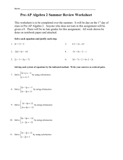
Figure 4.1. Illustration of the piecewise constant (donor-cell) advection algorithm.
Since we (by definition of the fact that we solve a numerical problem) do not know exactly what
this average state is, it is the task of the algorithm to provide a recipe that estimates this as well
as possible. In the two examples below we shall describe two such algorithms.
4.2 Donor-cell advection
The simplest flux conserving scheme is the donor-cell scheme. In this scheme the “average
interface state” is simply:
n
qi
for ui+1/2 > 0
n+1/2
q˜i+1/2 =
(4.14)
n
qi+1
for ui+1/2 < 0
This means that the donor-cell interface flux is:
ui+1/2 qin
n+1/2
fi+1/2 =
n
ui+1/2 qi+1
for ui+1/2 > 0
for ui+1/2 < 0
(4.15)
The physical interpretation of this method is the following. One assumes that the density is
constant within each cell. We then let the material flow through the cell interfaces, from left to
right for ui+1/2 > 0. Since the density to the left of the cell interface is constant, and since the
CFL condition makes sure that the flow is no further than 1 grid cell spacing at maximum, we
know that for the whole time between time tn and tn+1 the flux through the cell interface (which
is q˜i+1/2 ui+1/2 ) is constant, and is equal to Eq. (4.15). Once the time step if finished, the state
in each cell has the form of a step function (Fig. 4.1). To get back to the original sub-grid model
we need to average the quantity q(x) out over each cell, to obtain the new qin+1 . This is what
happens in the donor-cell algorithm.
This method is very strongly similar to the upstream differencing scheme of Section 3.3.2.
The difference comes to light mainly when either the velocity u is space-dependent or the grid
xi is non-constantly spaced (see Section 4.1.2). The Donor-Cell algorithm is easily implemented
but, as the upstream differencing method, it is very diffusive.
63
→ Exercise: Quantify the difference between the donor-cell and upstream differencing schemes
for non-constant grid spacing by writing the expressions for q n+1 in both cases and comparing them.
4.3 Piecewise linear schemes
The donor-cell algorithm is a simple algorithm based on the idea that at the beginning of each
time step the state within each cell is constant throughout the cell. The state at the grid center is therefore identical to that in the entire cell. The idea that the state is constant in the cell
is, however, just an assumption. One must make some assumption, because evidently we have
not more information about the state in the cell than just the cell-center state. But one could
also make another assumption. One could, for instance, assume that the state within each cell
is a linear function of position. One says that the state is assumed to be piecewise linear (see
Fig. 4.2). The assumption that it is a linear function within the cell is called a subgrid model: it is
a model of what the state looks like at spatial scales smaller than the grid spacing. The procedure
of creating a subgrid model based on a discrete value at the cell center is called reconstruction.
The piecewise linear scheme we discuss here is therefore a scheme based on piecewise linear
reconstruction of the function from the discrete values. Such a method, and higher order versions (such as the piecewise parabolic reconstruction discussed in a later chapter) are sometimes
called MUSCL (”Monotonic Uwind-centered Scheme for Conservation Laws”) schemes after
the original method of this kind proposed by van Leer (1977).
Within each cell the state at the beginning of the time step is now given by
q(x, t = tn ) = qin + σin (x − xi )
forxi−1/2 < x < xi+1/2
(4.16)
where σin is some slope, which we shall discuss below. We should assure that
1
xi = (xi−1/2 + xi+1/2 )
2
(4.17)
so that the state qin is equal to the average of q(x, t = tn ) over the cell irrespective of the slope
σin . This is necessary for flux conservation.
Let us, from here on, assume that the grid is equally spaced, i.e. that there is a global ∆x.
Let us also assume that u > 0 is a constant.
At the interface the flux will now vary with time between tn and tn+1 :
fi−1/2 (t) = uq(x = xi−1/2 , t)
n
n
= uqi−1
+ uσi−1
(xi−1/2 − xi−1 − u(t − tn ))
1
n
n
= uqi−1 + uσi−1
∆x − u(t − tn )
2
(4.18)
and similar for fi+1/2 (t). The average flux over the time step ∆t = (tn+1 − tn ) is then:
t
hfi−1/2 (t)itn+1
n
1
=
∆t
=
Z
tn+1
uq(x = xi−1/2 , t)dt
tn
n
uqi−1
1 n
(∆x − u∆t)
+ uσi−1
2
(4.19)
64
q
x
q
x
q
x
Figure 4.2. Illustration of the piecewise linear advection algorithm. The slope is chosen according to Lax-Wendroff’s method.
and similar for fi+1/2 (t). The difference is:
1
t
t
n
n
hfi+1/2 (t)itn+1
− hfi−1/2 (t)itn+1
) + u(σin − σi−1
= u(qin − qi−1
)(∆x − u∆t)
n
n
2
(4.20)
Using Eq. (4.10) we then obtain the update of the state after one time step:
qin+1 = qin −
u∆t 1 n
u∆t n
n
n
(qi − qi−1
)−
(σ − σi−1
)(∆x − u∆t)
∆x
∆x 2 i
n+1/2
(4.21)
t
where we defined fi+1/2 ≡ hfi+1/2 (t)itn+1
. Eq. (4.21) is the update of the state for a fluxn
conserving piecewise linear scheme (assuming that the grid spacing is constant). This is the
higher-order version of the donor-cell algorithm. Note that it is identical to donor-cell if the
slopes are chosen to be zero. Note also that since we chose the grid to be constantly spaced and
the velocity to be globally constant, the algorithm is like an upwind scheme with a correction
term.
The question is now: how shall we choose the slope σin of the linear function? The idea
behind the piecewise linear scheme is that one uses the states at adjacent grid points in some
reasonable way. There are three obvious methods:
n −q n
qi+1
i−1
2∆x
n
n
q −q
= i ∆xi−1
q n −q n
= i+1∆x i
Centered slope:
σin =
Upwind slope:
σin
Downwind slope:
σin
(Fromm’s method)
(4.22)
(Beam-Warming method)
(4.23)
(Lax-Wendroff method)
(4.24)
All these choices result in second-order accurate methods.
→ Exercise: Prove that the piecewise linear scheme with a downwind slope indeed produces
the Lax-Wendroff scheme of Eq. (3.96) in Chapter 3.
65
q
q
x
x
Figure 4.3. Illustration of why higher order schemes, such as the piecewise linear LaxWendroff scheme shown here, produce oscillations near discontinuities.
If we now implement, for instance, Fromm’s choice of slope into Eq. (4.21) then we obtain
the following explicit update of the state (again, valid only for regular grid spacing and constant
u):
u∆t n
n
n
(q + 3qin − 5qi−1
+ qi−2
)
4∆x i+1
u2 ∆t2 n
n
n
(qi+1 − qin − qi−1
+ qi−2
)
−
2
4∆x
qin+1 =qin −
(4.25)
This is called Fromm’s method of advection. One notices that the stencil of this scheme involves
4 points, and that these points are non-symmetric with respect to the updated cell. Only for the
downwind slope we regain a 3-point stencil.
4.4 Slope limiters: non-linear tools to prevent overshoots
As we have already seen in chapter 3 higher order schemes tend to produce oscillations near
jumps. We have seen that this can mathematically be understood in terms of phase errors and
dispersion. With the current piecewise linear geometric picture of the higher order methods we
can now also gain a geometrical understanding of why such an overshoot occurs. This is shown
in Fig. 4.3
In this picture the overshoot happens because the piecewise linear elements can have overshoots. A succesful method to prevent such overshoots is the use of slope limiters. These are
non-linear conditions that modify the slope σin if, and only if, this is necessary to prevent overshoots. This means that, if this is applied to for instance the Lax-Wendroff method, the slope
limiter keeps the second order nature of the Lax-Wendroff method in regions of smooth variation
of q while it will intervene whenever an overshoot threatens to take place.
4.4.1 The “Total Variation” (TV)
To measure oscillations in a solution we define the Total Variation (TV) of the discrete representation of q to be:
N
X
T V (q) =
|qi − qi−1 |
(4.26)
i=1
where i = 1 and i = N are the left and right boundaries of the numerical grid respectively. For a
monotonically increasing function q the T V (q) = |q1 −qN |. If q1 and qN are taken to be constant,
then, as long as the function remains monotonic, the T V (q) is constant. However, if the values
of qi develop local minima or maxima, then the T V increases, by virtue of the absolute value in
Eq. (4.26). The increase of T V is therefore a measure of the development of oscillations in a
solution.
66
q
q
x
x
minmod slope
superbee slope
Figure 4.4. Illustration of the slope limites minmod and superbee. Both clearly prevent overshoots in the subgrid models and hence are TVD.
A numerical scheme is said to be total variation diminishing (TVD) if:
T V (q n+1 ) ≤ T V (q n )
(4.27)
Clearly such a scheme will not develop oscillations near a jump, because a jump is a monotonically in/decreasing function and a total variation diminishing scheme will not increase the T V ,
and hence in this case keep the T V identically constant. This appears to be a desirable property
of the numerical scheme.
What about if we already start with a solution that has some local minima and maxima?
In principle a total variation diminishing scheme could conserve the total variation (as long as
it does not increase it). In practice, however, the local minima and maxima will be gradually
smoothed out by such a scheme. Good schemes will do this only very weakly, and will only
really diminish oscillations near sharp jumps.
4.4.2 Slope limiters
So now let us try to formulate a recipe to limit the slope σin of the piecewise linear scheme to
make sure that the resulting scheme is TVD. One obvious choise is to take the slope always zero.
We then recover the donor-cell algorithm. This algorithm is TVD because the piecewise constant
function has the same TV as the continuous function. In fact, as we have discussed in Section
3.9, all first order schemes are TVD.
For the piecewise linear scheme there are several methods to guarantee TVD. One method
is the minmod slope:
n
n
n
qi − qi−1
qi+1
− qin
n
σi = minmod
(4.28)
,
δx
δx
where

if |a| < |b| and ab > 0
a
if |a| > |b| and ab > 0
minmod(a, b) = b
(4.29)

0
if ab ≤ 0
This method chooses the smallest of the two slopes, provided they both have the same sign, and
chooses 0 otherwise. The minmod slope is illustrated in Fig. 4.4-left.
Another efficient slope limiter is the superbee slope limiter introduced by Phil Roe:
(1)
(2)
σin = maxmod(σi , σi )
(4.30)
with
(1)
σi
(2)
σi
n
n
qi+1
− qin qin − qi−1
= minmod
,2
δx
δx
n
n
n
n
qi+1 − qi qi − qi−1
= minmod 2
,
δx
δx
(4.31)
(4.32)
67
Figure 4.5. Advection with the piecewise linear advection algorithm with 6 different choices
of the slope. Results are shown of the advection of a step function over a grid of 100 points
with grid spacing ∆x = 1, after 300 time steps with ∆t = 0.1.
The superbee slope is shown in Fig. 4.4-right.
In Fig. 4.5 the results are shown for all the piecewise linear advection algorithms discussed
here.
4.5 Flux limiters
The concept of slope limiters is very closely related to the concept of flux limiters. For fluxconserving schemes the concept of flux-limiter is more appropriate and can be better implemented. Let us take another look at the time-averaged flux through a cell interface (Eq. 4.19).
For arbitrary sign of u this becomes:
 n
n
∆x − ui−1/2 ∆t
if ui−1/2 ≥ 0
uqi−1 + 12 ui−1/2 σi−1
n+1/2
(4.33)
fi−1/2 =

1
n
n
uqi − 2 ui−1/2 σi ∆x + ui−1/2 ∆t
if ui−1/2 ≤ 0
68
t
where we dropped the hitn+1
for notational convenience and put instead a n+1/2 to denote the fact
n
that the flux average is similar to taking the flux at half-time1. We have also now allowed for a
varying velocity u. The velocity u is, in this formulation, defined on the cell interfaces, while
the value of q is always defined at the cell center. If we, for convenience, introduce
+1
for ui−1/2 ≥ 0
(4.34)
θi−1/2 ≡ θ(ui−1/2 ) =
−1
for ui−1/2 ≤ 0
then we can write
i
h
1
n+1/2
n
n
fi−1/2 = ui−1/2 (1 + θi−1/2 )qi−1 + (1 − θi−1/2 )qi +
2
i
h
ui−1/2 ∆t 1
n
n
∆x (1 + θi−1/2 )σi−1
+
(1
−
θ
)σ
|ui−1/2 | 1 − i−1/2 i
4
∆x (4.35)
This expression is identical to Eq. (4.33). It is just written in a single formula using the flipflop function θi−1/2 which is +1 for positive advection velocity and −1 for negative advection
velocity. This expression is valid for any regularly or non-regularly spaced grid, and for any
constant or varying advection velocity. It is therefore the kind of expression we need for numerical hydrodynamics in which non-regular grids and, more importantly, varying velocity fields are
common.
In Eq. (4.35) it is now possible to replace
i
1 h
n
n
n
→ φ(ri−1/2
)(qin − qi−1
)
(4.36)
∆x (1 + θi−1/2 )σi−1
+ (1 − θi−1/2 )σin
2
n
n
where we introduced a flux limiter φ(ri−1/2
) where ri−1/2
is defined as:
 qi−1
n −q n
i−2
for ui−1/2 ≥ 0

n
 qin −qi−1
n
ri−1/2
=
n −q n

 qi+1
i
for ui−1/2 ≤ 0
n
q −q n
i
We shall discuss expressions for
modified by this replacement:
n
φ(ri−1/2
)
(4.37)
i−1
in a minute, but first let us see how Eq. (4.35) is
h
i
1
n+1/2
n
fi−1/2 = ui−1/2 (1 + θi−1/2 )qi−1
+ (1 − θi−1/2 )qin +
2
ui−1/2 ∆t 1
n
n
φ(ri−1/2
)(qin − qi−1
)
|ui−1/2 | 1 − 2
∆x (4.38)
We see that this expression of the flux is still the donor-cell flux (first line) plus some correction
term (second line).
We can now verify that with particular choices of the flux limiter function φ(r) we regain
the various recipes of Section 4.4:
donor-cell :
Lax-Wendroff :
Beam-Warming :
Fromm :
1
φ(r) = 0
φ(r) = 1
φ(r) = r
φ(r) = 21 (1 + r)
(4.39)
Note, however, that this does not mean that we have a Crank-Nicholson scheme here! This is not an implicit
scheme!
69
which are the linear schemes and
minmod :
superbee :
φ(r) = minmod(1, r)
φ(r) = max(0, min(1, 2r), min(2, r))
(4.40)
which are the high-resolution non-linear schemes. Now that we are at it, there are also many
other non-linear flux limiter schemes. Two examples are:
MC :
van Leer :
φ(r) = max(0, min((1 + r)/2, 2, 2r))
φ(r) = (r + |r|)/(1 + |r|)
(4.41)
where MC stands for monotonized central-difference limiter.
A flux limiter has the following effect:
• For smooth parts of a solution it will do second order accurate flux-conserved advection.
• For regions near a jump or a very sharp and sudden gradient it will switch to first order
donor-cell (i.e. upwind) flux-conserved advection.
Flux limiters therefore make sure that one gets the best of both second order and first order
methods. Flux limiters will turn out to play a major role for shock capturing hydrodynamics
codes, in which shocks need to be kept tight and not smear out over too many grid cells. For the
modeling of supersonic flows with shock waves (such as those often found in astrophysics) they
are a highly useful tool. However, one should keep in mind that they may artificially steepen
gradients that may not actually be meant to be steepened. They therefore have to be used with
care.
4.6 Overview of algorithms
As a final remark we give here a table of the properties of the various algorithms:
Name
Order
Lin?
Stable? TVD? Stencil
Two-point symmetric
1
lin
-
-
Upwind / Donor-cell
1
lin
+
+
Lax-Wendroff
2
lin
+
-
Beam-warming
2
lin
+
-
Fromm
2
lin
+
-
Minmod
2/1
non-lin
+
+
Superbee
2/1
non-lin
+
+
MC
2/1
non-lin
+
+
van Leer
2/1
non-lin
+
+
70
4.7 Computer implementation (adv-2): cell interfaces and ghost cells
The computer implementation is now a bit more complicated than in chapter 3 because we now
have cells, and cell-interfaces. In this section we will see how to deal with this in a proper way.
Also we will introduce the concept of ghost cells which is a simple trick to implement boundary
conditions in a very easy way, even periodic boundary conditions. It will help us greatly when
we will do the hydrodynamics in the later chapters.
Let us, as in the previous section, set up the problem in IDL/GDL. First the grid:
nx
x
xi
= 100
= dblarr(nx+2)
= dblarr(nx+3)
Here we have 100 regular grid points with a ghost cell on each side. We have therefore 102 cells
with 103 cell walls. We now also define the array for q, for the temporary array qnew and for
the flux f :
q
qnew
f
= dblarr(nx+2)
= dblarr(nx+2)
= dblarr(nx+3)
Now we set up the grid
dx
= 1.d0
; Set grid spacing
for i=0,nx+1 do x[i] = (i-1.d0) * dx
for i=1,nx+1 do xi[i] = 0.5 * ( x[i] + x[i-1] )
xi[0]
= x[0] - 0.5 * ( x[1] - x[0] )
xi[nx+2] = x[nx+1] + 0.5 * ( x[nx+1] - x[nx] )
where we made the grid regular with grid spacing dx. Note that the cell walls are indexed such
that wall i is left of cell i (see Fig. 4.6). Now we set up the initial condition and the advection
velocity array
for i=0,nx-1 do if x[i] lt 30. then q[i]=1.d0 else q[i]=0.d0
u
= 1.d0 + dblarr(nx+3)
Note that the advection velocity array is also defined on the cell walls. Now the main part of the
code is:
dt
= 2d-1
tend
= 70.d0
time
= 0.d0
while time lt tend do begin
;;
;; Check if end time will not be exceeded
;;
if time + dt lt tend then begin
dtused = dt
endif else begin
dtused = tend-time
endelse
71
;;
;; Impose cyclic (=periodic) boundary conditions
;; using the ghost cells
;;
q[0]
= q[nx]
q[nx+1] = q[1]
;;
;; Make the flux
;;
for i=1,nx+1 do begin
if u[i] gt 0 then begin
f[i] = q[i-1] * u[i]
endif else begin
f[i] = q[i] * u[i]
endelse
endfor
;;
;; Do the advection
;;
for i=1,nx do begin
qnew[i] = q[i] - dtused * ( f[i+1] - f[i] ) / $
( xi[i+1]- xi[i] )
endfor
;;
;; Copy back
;;
for i=1,nx do begin
q[i] = qnew[i]
endfor
;;
;; Update time
;;
time = time + dtused
endwhile
Here we have imposed cyclic (periodic) boundary conditions, just as an example how useful
ghost cells can be. We have also made sure that the algorithm works for any u(x), also if it is a
function of x and if it changes sign. If we now end the program with
plot,x[1:nx],q[1:nx],psym=-6
end
then we will see a figure on the screen like Fig. 4.7. Note that the periodic boundary conditions
have the effect that the diffusive smearing now affects the front- and the back-side of the block
function, in contrast to the case of Fig. 3.6. Also note that in the present program we went all the
way to t = 70 instead of t = 30 of Fig. 3.6. The smearing has now almost entirely destroyed the
block function.
72
Domain of interest
Ghost
cell
Ghost
cell
0
1
−1/2
1/2
0
2
1
0
3
3/2
1
5/2
2
3
2
3
nx
4
7/2
9/2
4
4
nx+1
nx+1/2 nx+3/2
Mathematical
indices
nx+1
Computer
indices
nx
nx
nx+1
nx+2
Domain of interest
Ghost
cell
Ghost
cell
−1
−3/2
0
−1/2
0
0
Ghost
cell
1
1/2
1
1
2
3/2
2
2
3
3
4
3
5/2
7/2
4
4
nx
9/2
nx
nx
nx+1
nx+2
nx+1/2 nx+3/2 nx+5/2
nx+1
nx+1
Ghost
cell
nx+2
nx+2
nx+3
nx+3
nx+4
Mathematical
indices
Computer
indices
Figure 4.6. The grid of a flux-conserving advection program including ghost cells, for algorithms with a three-point stencil (upper panel) and for algorithms with a four- or five-piont
stencil (lower panel).
Figure 4.7. The plot resulting from the donorcell.pro program of Section 4.7. Note that in
contrast to Fig. 3.6 we now have continued the simulation until time t = 70 and we have
imposed periodic boundary conditions. Hence the difference to Fig. 3.6.