1. business and industrial
2. company
3. bankruptcy

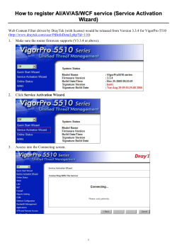
PLAXIS implementation of HYPOPLASTICITY
including standalone ABAQUS umat subroutines
David Maˇs´ın
January 20, 2015
Chapter 1
INTRODUCTION
This page is a part of a research project www.soilmodels.info. The aim of this page
is to provide user defined subroutine umat for the hypoplastic constitutive models,
together with an interface for PLAXIS user defined subroutine UsrMod.
1
Chapter 2
IMPLEMENTED MODELS LITERATURE SOURCES
For details of material models available at this web site in the form of finite element
implementation, the interested readers are referred to the journal publications. The
following literature sources are relevant:
1. Sand hypoplasticity model:
Model formulation is described in von Wolffersdorff (1996) [?]. For details of
model calibration procedure, see Herle and Gudehus (1999) [?]. Small strain
stiffness formulation (so-called intergranular strain concept) is described in
Niemunis and Herle (1997) [?].
2. Clay hypoplasticity model:
The implemented model has been published by Maˇs´ın (2013) [?]. This model
is an anisotropic version of the general clay hypoplasticity model described
thoroughly in Maˇs´ın [?]. Structure of the anisotropic stiffness matrix described
in Maˇs´ın and Rott [?]. Structured-soil specific model features are described
in Maˇs´ın (2007) [?]. The model can be used with the intergranular strain
concept, its original formulation is in Niemunis and Herle (1997) [?], enhanced
formulation implemented is in Maˇs´ın (2013) [?]. Most of the cited journal
papers available here for free download in the form of PDF preprints.
Further details on calibration of material parameters of hypoplastic models can be
found here.
2
Chapter 3
TIME INTEGRATION
Constitutive models are integrated using explicit adaptive integration scheme with
local substepping. The constitutive model forms an ordinary differential equation of
the form
dy
= f (t, y)
dt
The equation is for finite time step size ∆t solved using the Runge-Kutta method.
Solutions that correspond to the second- and third- order accuracy of Taylor series
expansion are given by
(2)
(3)
y(t+∆t)
y(t+∆t) = y(t) + k2
1
= y(t) + (k1 + 4k2 + k3 )
6
where
k1 = ∆t f t, y(t)
∆t
k1
k2 = ∆t f t +
, y(t) +
2
2
k3 = ∆t f t + ∆t, y(t) − k1 + 2k2
The accuracy of the solution is estimated following Fehlberg as the difference
between the second- and third- order solutions. The time step size ∆t is accepted, if
(3)
(2)
err = y(t+∆t) − y(t+∆t) < T OL
(3)
where T OL is a prescribed error tolerance. If the step-size ∆t is accepted, y(t+∆t) is
considered as a solution for the given time step and the new time step size ∆tn is
3
CHAPTER 3. TIME INTEGRATION
estimated according to Hull
"
∆tn = min 4∆t, 0.9∆t
T OL
err
1/3 #
If the step-size ∆t is not accepted, the step is re-computed with new time step size
"
1/3 #
T
OL
∆t
, 0.9∆t
∆tn = max
4
err
In the case the prescribed minimum time step size or the prescribed maximum number of time substeps is reached, the finite element program is asked to reject the
current step and to decrease the size of the global time step.
4
Chapter 4
INPUT OF PARAMETERS AND
STATE VARIABLES IN PLAXIS
4.1
Hypoplastic model for granular materials
Parameters are specified in the PLAXIS input in the following order:
• Parameter 1 – critical state friction angle ϕc
• Parameter 2 – pt – shift of the mean stress due to cohesion. The effective stress
σ used in the model formulation is replaced by σ − 1pt . Non-zero value of
pt is needed to overcome problems with stress-free state. If pt = 0, it will be
replaced by a default value of 1 kPa. Any other value can be input by user (for
basic hypoplasticity, set pt to very low number, e.g. pt = 1.e − 5).
• Parameters 3-9 – parameters of the basic hypoplastic model for granular materials hs , n, ed0 , ec0 , ei0 , α, β.
• Parameters 10-14 – the intergranular strain concept parameters (mR , mT , R,
βr , χ). If mR = 0 the intergranular strain concept is switched off and the
problem is simulated using the basic hypoplastic model.
• Parameter 15 – not used.
• Parameter 16 – initial void ratio corresponding to the zero mean stress e0 or
initial void ratio e. If P ar(16) < 10, then e is calculated from the mean stress
p and from e0 = P ar(16) using Bauer [?] formula. If P ar(16) > 10, then
e = P ar(16) − 10.
5
4.1. HYPOPLASTIC MODEL FOR GRANULARCHAPTER
MATERIALS
4. PLAXIS INPUT
• Parameters 17-22 – initial values of the intergranular strain tensor δ in Voigt
notation (δ11 , δ22 , δ33 , 2δ12 , 2δ13 , 2δ23 ).
State variables:
The routine uses 14 state variables:
• State v. 1-6 – intergranular strain tensor δ in Voigt notation (δ11 , δ22 , δ33 , 2δ12 ,
2δ13 , 2δ23 ).
• State v. 7 – void ratio e.
• State v. 8 – not used.
• State v. 9 – Effective mean stress.
• State v. 10 – Number of evaluation of the constitutive model in one global
time step (for postprocessing only).
• State v. 11 – Mobilised friction angle ϕmob in degrees (for postprocessing only).
• State v. 12 – Normalised length ρ of the intergranular strain tensor δ (for
postprocessing only).
• State v. 13 – Suggested size of the first time substep (for calculation controll).
• State v. 14 – free.
The hypoplastic model for granular materials is implemented via user defined
subroutine usermod. To use the model in PLAXIS, copy the files UDSM HPS.dll
and UDSM HPS64.dll into the PLAXIS installation directory. Then, select ”userdefined model” from the Material model combo box in the General tab sheet (Fig.
4.1). (Fig. 4.1). After selecting the user-defined model, correct user-defined dynamic
library (typically UDSM HPS.dll) needs to be selected in the ”Available DLL’s”
combo box under ”Parameters” tab sheet. In the ”Models in DLL” combo box,
model with ID 1 (Hypoplas. - sand) must be selected. The parameters can then be
input into the parameter table (Fig. 4.2).
Parameters of the sand hypoplastic model for different soils have been evaluated by Herle and Gudehus [?]. They are given in Table 4.1. Parameters of the
intergranular strain concept for granular materials are in Tab. 4.2.
6
4.2. HYPOPLASTIC MODEL FOR CLAYS
CHAPTER 4. PLAXIS INPUT
Figure 4.1: Selecting user defined model in the Material model combo box.
4.2
Hypoplastic model for clays
Parameters are specified in the PLAXIS input in the following order:
Parameters:
• Parameter 1 – critical state friction angle ϕc
• Parameter 2 – pt – shift of the mean stress due to cohesion. The effective stress
σ used in the model formulation is replaced by σ − 1pt . Non-zero value of
pt is needed to overcome problems with stress-free state. If pt = 0, it will be
replaced by a default value of 1 kPa. Any other value can be input by user (for
basic hypoplasticity, set pt to very low number, e.g. pt = 1.e − 5).
• Parameters 3-5 – parameters of the basic hypoplastic model for clays λ∗ , κ∗ ,
N.
• Parameters 6 – Parameters of the basic hypoplastic model for clays νpp (in
place of the parameter r of the Maˇs´ın (2005) [?] model, calibrated using the
same procedure).
7
4.2. HYPOPLASTIC MODEL FOR CLAYS
CHAPTER 4. PLAXIS INPUT
Figure 4.2: Selecting sand hypoplasticity model in the ”Parameters” tab sheet.
• Parameters 7 – αG , ratio of horisontal and vertical shear moduli.
• Parameters 8-10 – parameters of the model for clays with meta-stable structure
(k, A and sf ).
• Parameters 11-13 – Intergranular strain concept parameters R, βr , χ.
• Parameters 14-15 – Very small strain shear stiffness parameters Ag and ng .
If Ag = 0 the intergranular strain concept is switched off and the problem is
simulated using the basic hypoplastic model.
• Parameters 16 – Intergranular strain concept parameter mrat .
• Parameter 17 – bulk modulus of water Kw for undrained analysis using the
penalty approach with user-defined value of Kw . In drained analysis, consolidation analysis, and undrained analysis using PLAXIS option undrained Kw
should be set to 0.
• Parameter 18 – Specifies vertical direction (set to 2 in PLAXIS2D, 3 in PLAXIS3D,
2 in SoilTest independently whether run from PX2D or PX3D).
8
4.2. HYPOPLASTIC MODEL FOR CLAYS
Hochstetten gravel
Hochstetten sand
Hostun sand
Karlsruhe sand
Lausitz sand
Toyoura sand
ϕc
36◦
33◦
31◦
30◦
33◦
30◦
hs
32 ×106 kPa
1.5 ×106 kPa
1.0 ×106 kPa
5.8 ×106 kPa
1.6 ×106 kPa
2.6 ×106 kPa
n
0.18
0.28
0.29
0.28
0.19
0.27
CHAPTER 4. PLAXIS INPUT
ed0
0.26
0.55
0.61
0.53
0.44
0.61
ec0
ei0
α
β
0.45 0.5 0.1 1.9
0.95 1.05 0.25 1.5
0.96 1.09 0.13 2
0.84
1
0.13 1
0.85
1
0.25 1
0.98 1.1 0.18 1.1
Table 4.1: Typical parameters of the hypoplastic model for granular materials (Herle
and Gudehus [?])
Hochstetten sand
R
mR
1.e-4 5.0
mT
2.0
βr χ
0.5 6
Table 4.2: Parameters of the intergranular strain concept for sandy soils (Niemunis
and Herle [?])
• Parameter 19 – Parameter αE (ratio of horizontal and vertical Young moduli).
If set to zero, than calculated automatically from empirical formulation αE =
(1/0.8)
.
αG
• Parameter 20 – Parameter αν (ratio of horizontal and vertical Poisson ratios). If
set to zero, than calculated automatically from empirical formulation αν = αG .
• Parameter 21 – Parameter αf . Additional control of non-linearity inside state
boundary surface. If set to zero, default value calculated from model parameters is used.
• Parameter 22 – initial void ratio e or overconsolidation ratio OCR. If P ar(19) <
10, then e = P ar(19). If P ar(19) > 10, then OCR = P ar(19) − 10.
• Parameters 23-28 – initial values of the intergranular strain tensor δ in Voigt
notation (δ11 , δ22 , δ33 , 2δ12 , 2δ13 , 2δ23 ).
• Parameter 29 – initial value of sensitivity (model for clays with meta-stable
structure). If s = 0, the basic model is used.
State variables:
The routine uses 14 state variables:
9
4.2. HYPOPLASTIC MODEL FOR CLAYS
CHAPTER 4. PLAXIS INPUT
• State v. 1-6 – intergranular strain tensor δ in Voigt notation (δ11 , δ22 , δ33 , 2δ12 ,
2δ13 , 2δ23 ).
• State v. 7 – void ratio e.
• State v. 8 – Excess pore pressure u for undrained analysis using user-defined
value of Kw . In undrained analysis using PLAXIS option undrained this variable is equal to 0 end excess pore pressure may be found in standard PLAXIS
menu.
• State v. 9 – Effective mean stress.
• State v. 10 – Number of evaluation of the constitutive model in one global
time step (for postprocessing only).
• State v. 11 – Mobilised friction angle ϕmob in degrees (for postprocessing only).
• State v. 12 – Normalised length ρ of the intergranular strain tensor δ (for
postprocessing only).
• State v. 13 – Suggested size of the first time substep (for calculation controll).
• State v. 14 – sensitivity s (for model with meta-stable structure).
• State v. 15 – overconsolidation ratio, defined as OCR = pe /p.
• State v. 16 – 0 means model interation goes without problem. 1 means state
boundary surface cut-off has been activated.
The hypoplastic model for granular materials is implemented via user defined
subroutine usermod. To use the model in PLAXIS, copy the files UDSM HPS.dll
and UDSM HPS64.dll into the PLAXIS installation directory. Then, select ”userdefined model” from the Material model combo box in the General tab sheet (Fig.
4.1). After selecting the user-defined model, correct user-defined dynamic library
(typically UDSM HPS.dll) needs to be selected in the ”Available DLL’s” combo box
under ”Parameters” tab sheet. In the ”Models in DLL” combo box, model with ID
2 (Hypoplas. - clay) must be selected. The parameters can then be input into the
parameter table (Fig. 4.3).
Parameters of the clay hypoplastic model for different soils have been evaluated
by Maˇs´ın and co-workers. They are given in Table 4.3. Parameters of the model
for clays with meta-stable structure are in Tab. 4.4 and typical parameters of the
intergranular strain concept for fine-grained soils are in Tab. 4.5.
10
4.2. HYPOPLASTIC MODEL FOR CLAYS
Brno clay
London clay
Kaolin
Dortmund clay
Weald clay
Koper silt
Fujinomori clay
Pisa clay
Beaucaire clay
Trmice clay
ϕc
22◦
21.9◦
27.5◦
27.9◦
24◦
33◦
34◦
21.9◦
33◦
18.7◦
λ∗
0.128
0.095
0.065
0.057
0.059
0.103
0.045
0.14
0.06
0.09
CHAPTER 4. PLAXIS INPUT
κ∗
N
νpp
αG
0.015 1.51 0.33 1.35
0.015 1.19 0.1
2
0.01 0.918 0.35
0.008 0.749 0.38
0.018 0.8
0.3
0.015 1.31 0.28
0.011 0.887 0.36
0.01 1.56 0.31
0.01 0.85 0.21
0.01 1.09 0.09
-
Table 4.3: Typical parameters of the hypoplastic model for clays.
For estimation of αG , see database from [?], here for free download in the form
of PDF preprint.
k
A sf
Pisa clay
0.4 0.1 1
Bothkennar clay 0.35 0.5 1
Table 4.4:
(from [?])
Typical parameters of the model for clays with meta-stable structure
London clay (data Gasparre)
Brno clay (nat.)
R
βr
χ
Ag
ng mrat
5.e-5 0.08 0.9 270
1
0.5
1e-4 0.2 0.8 5300 0.5 0.5
Table 4.5: Typical parameters of the intergranular strain concept for clays
11
4.2. HYPOPLASTIC MODEL FOR CLAYS
CHAPTER 4. PLAXIS INPUT
12
Figure 4.3: Selecting clay hypoplasticity model in the ”Parameters” tab sheet.
Chapter 5
EXAMPLES
5.1
Excavation in sand
The example of the excavation is taken over from PLAXIS manual; the problem is
simulated with sand hypoplasticity model. Soil parameters of the sand correspond
to the Hochstetten sand from Tab. 4.1; the intergranular strain parameters used are
in Tab. 4.2. The sand is in a medium dense state with e0 =0.85.
Fig. 5.1 shows total displacements. Fig. 5.2 shows the normalised length of
the intergranular strain tensor. The normalised length of the intergranular strain
tensor varies between 0, which indicates the soil being inside the elastic range, and
1, corresponding to the state swept-out of the small-strain memory. In the case of the
normalised length of the intergranular strain being equal to 1 the soil behaviour is
governed by the basic hypoplastic model. Indeed, Fig. 5.2 shows that this is the case
of an excavation, the soil below the bottom of the excavation and behind the wall
is outside the small-strain-stiffness range. Fig. 5.3 shows mobilised friction angle,
indicating emerging failure mechanism.
Input file for this example may be downloaded in Sec. 8.
13
5.2. NATM TUNNEL IN CLAY
CHAPTER 5. EXAMPLES
Figure 5.1: Excavation in sand - total displacement.
5.2
NATM tunnel in clay
In this example, an NATM tunnel excavated in stiff clay is simulated. The clay is
simulated with London clay parameters (Tab. 4.3 for parameters of the basic model;
Tab 4.5. for the intergranular strain parameters), with the initial value of void ratio
equal to 0.7.
Figure 5.4 shows the displacement field predicted by the anisotropic stiffness
model with αG = 2, whereas 5.5 shows the displacement field predicted by the model
with αG = 1. Clearly, the anisotropic model predicts narrower and deeper surrface
settlement trough, which agrees better with monitored data. This is also clear from
the settlement trough shown in Fig. 5.6. There, also predictions by the Maˇs´ın (2005)
model [?] are included, which are close to the predictions by the isotropic model. Fig.
5.7 shows the normalised length of the intergranular strain tensor. The normalised
length of the intergranular strain tensor in Fig. 5.7 demonstrates how the small-strain
stiffness is activated in different parts of the modelled geometry.
14
5.3. BUILDING SUBJECTED TO AN EARTHQUAKE
CHAPTER 5. EXAMPLES
Figure 5.2: Excavation in sand - normalised length of the intergranular strain tensor.
5.3
Building subjected to an earthquake
This example demonstrates capabilities of a hypoplastic model in dynamic analysis of the earthquake impact on existing infrastructure. A real accelerogram of an
earthquake recorded by USGS in 1989 is used for the analysis.
The building consists of 4 floors and a basement. It is 6 m wide and 25 m
high. The subsoil consists of a sand with water level reaching the surface. The
soil behaviour during the earthquake is considered as undrained. Two cases were
simulated. In one case, the soil is in a loose state (e0 = ec0 ), in the second case
the soil is in a dense state (e0 is close to ed0 ). Hypoplastic model parameters of the
Hochstetten sand from Tab. 4.1 and the intergranular strain parameters from Tab.
4.2 are adopted.
Overall displacements of the top of the building are shown in Fig. 5.8. The soil
response to the earthquake depends significantly on the soil state. The loose soil
liquefies after 3-4 s of the earthquake, leading to the failure. The analysis cannot
15
5.3. BUILDING SUBJECTED TO AN EARTHQUAKE
CHAPTER 5. EXAMPLES
Figure 5.3: Excavation in sand - mobilised friction angle.
continue and fails. The displacements are much lower in the case of dense soil.
Although some displacements occur also in this case, the soil retains some bearing
capacity sufficient to overcome the failure.
Figure 5.9 shows total displacements after approx. 4 s of earthquake for the loose
soil case, whereas Figure 5.10 shows the displacements at the same time (and in the
same scale) for the dense soil. The figures indicate foundation failure for the loose
soil case and relatively low displacements for the dense soil case.
16
5.3. BUILDING SUBJECTED TO AN EARTHQUAKE
CHAPTER 5. EXAMPLES
Figure 5.4: NATM tunnel construction - vertical displacement field predicted by the
anisotropic model.
17
5.3. BUILDING SUBJECTED TO AN EARTHQUAKE
CHAPTER 5. EXAMPLES
Figure 5.5: NATM tunnel construction - vertical displacement field predicted by the
isotropic model.
18
5.3. BUILDING SUBJECTED TO AN EARTHQUAKE
CHAPTER 5. EXAMPLES
Figure 5.6: NATM tunnel construction - surface settlement troughs predicted by
different models.
19
5.3. BUILDING SUBJECTED TO AN EARTHQUAKE
CHAPTER 5. EXAMPLES
Figure 5.7: NATM tunnel construction - normalised length of the intergranular strain
tensor.
20
5.3. BUILDING SUBJECTED TO AN EARTHQUAKE
CHAPTER 5. EXAMPLES
Figure 5.8: Displacement of the top of the building during the earthquake.
21
5.3. BUILDING SUBJECTED TO AN EARTHQUAKE
CHAPTER 5. EXAMPLES
Figure 5.9: Total displacements after 4 s of earthquake - loose soil.
Figure 5.10: Total displacements after 4 s of earthquake - dense soil.
22
Chapter 6
TROUBLESHOOTING
Although the implementation has been tested to be accurate and robust, the hypoplastic models are highly non-linear which may cause problems during solving
complex boundary value problems. When encountering problems, the following steps
may help to improve the overall performance:
1. In the ”Iterative procedure” settings under ”Parameters” Tab sheet, set ”Manual settings” and do not use the arc-length control.
2. Try to modify the iterative procedure by decreasing the ”Desired minimum”
and ”Desired maximum” number of iterations (for example, 3 and 5 respectively).
3. The hypoplastic models are undefined in the tensile stress region, which can
cause integration problems in the vicinity of the free surface and in the case of
staged construction starting from the stress-free state. For this reason, artificial
cohesion is introduced in the model implementation through the parameter pt .
The user can specify any pt value; in the case pt =0 kPa, the program replaces
it by a default value pt =1 kPa.
4. When used with interface elements, proper interface parameters must be input
in the ”Interface” Tab sheet under ”Material models” window. Particularly, as
some tensile stress is allowed for in the soil through the parameter pt , the tensile
stress should be allowed for also in the interface by increasing the cohesion value
(e.g., 10 kPa). Convergence problems may also be caused by high interface
stiffness. In the case PLAXIS keeps on iterating although the global error
is below the tolerated value, or does not increase the step size although the
23
CHAPTER 6. TROUBLESHOOTING
number of iterations is below the ”desired minimum”, problem is the most
likely in interfaces.
24
Chapter 7
ACKNOWLEDGEMENT
The RKF-23 time integration scheme was programmed and kindly provided by Prof.
C. Tamagnini and E. Sellari. The original umat - PLAXIS interface, which served as
a basis for the present developments, was programmed and kindly provided by Dr.
P.-A. von Wolffersdorff. The implementation was optimised during the stay of the author at Plaxis bv in March 2010. Plaxis support is greatly appreciated. Development
of constitutive models was supported by the research grant GACR 205/08/0732.
Software was developed under support of grant TACR TA01031840.
25
Bibliography
26
Chapter 8
DOWNLOAD
27
Chapter 9
GNU GENERAL PUBLIC
LICENSE
GNU GENERAL PUBLIC LICENSE Version 2, June 1991
Copyright (C) 1989, 1991 Free Software Foundation, Inc. 59 Temple Place, Suite
330, Boston, MA, 02111-1307, USA Everyone is permitted to copy and distribute
verbatim copies of this license document, but changing it is not allowed.
Preamble
The licenses for most software are designed to take away your freedom to share
and change it. By contrast, the GNU General Public License is intended to guarantee
your freedom to share and change free software–to make sure the software is free for
all its users. This General Public License applies to most of the Free Software
Foundation’s software and to any other program whose authors commit to using
it. (Some other Free Software Foundation software is covered by the GNU Library
General Public License instead.) You can apply it to your programs, too.
When we speak of free software, we are referring to freedom, not price. Our
General Public Licenses are designed to make sure that you have the freedom to
distribute copies of free software (and charge for this service if you wish), that you
receive source code or can get it if you want it, that you can change the software or
use pieces of it in new free programs; and that you know you can do these things.
To protect your rights, we need to make restrictions that forbid anyone to deny
you these rights or to ask you to surrender the rights. These restrictions translate
to certain responsibilities for you if you distribute copies of the software, or if you
modify it.
For example, if you distribute copies of such a program, whether gratis or for a
fee, you must give the recipients all the rights that you have. You must make sure
28
CHAPTER 9. GNU GENERAL PUBLIC LICENSE
that they, too, receive or can get the source code. And you must show them these
terms so they know their rights.
We protect your rights with two steps: (1) copyright the software, and (2) offer
you this license which gives you legal permission to copy, distribute and/or modify
the software.
Also, for each author’s protection and ours, we want to make certain that everyone
understands that there is no warranty for this free software. If the software is modified
by someone else and passed on, we want its recipients to know that what they have
is not the original, so that any problems introduced by others will not reflect on the
original authors’ reputations.
Finally, any free program is threatened constantly by software patents. We wish
to avoid the danger that redistributors of a free program will individually obtain
patent licenses, in effect making the program proprietary. To prevent this, we have
made it clear that any patent must be licensed for everyone’s free use or not licensed
at all.
The precise terms and conditions for copying, distribution and modification follow.
GNU GENERAL PUBLIC LICENSE TERMS AND CONDITIONS FOR COPYING, DISTRIBUTION AND MODIFICATION
0. This License applies to any program or other work which contains a notice
placed by the copyright holder saying it may be distributed under the terms of this
General Public License. The ”Program”, below, refers to any such program or work,
and a ”work based on the Program” means either the Program or any derivative work
under copyright law: that is to say, a work containing the Program or a portion of
it, either verbatim or with modifications and/or translated into another language.
(Hereinafter, translation is included without limitation in the term ”modification”.)
Each licensee is addressed as ”you”.
Activities other than copying, distribution and modification are not covered by
this License; they are outside its scope. The act of running the Program is not
restricted, and the output from the Program is covered only if its contents constitute
a work based on the Program (independent of having been made by running the
Program). Whether that is true depends on what the Program does.
1. You may copy and distribute verbatim copies of the Program’s source code as
you receive it, in any medium, provided that you conspicuously and appropriately
publish on each copy an appropriate copyright notice and disclaimer of warranty; keep
intact all the notices that refer to this License and to the absence of any warranty;
and give any other recipients of the Program a copy of this License along with the
Program.
29
CHAPTER 9. GNU GENERAL PUBLIC LICENSE
You may charge a fee for the physical act of transferring a copy, and you may at
your option offer warranty protection in exchange for a fee.
2. You may modify your copy or copies of the Program or any portion of it, thus
forming a work based on the Program, and copy and distribute such modifications
or work under the terms of Section 1 above, provided that you also meet all of these
conditions:
a) You must cause the modified files to carry prominent notices stating that you
changed the files and the date of any change.
b) You must cause any work that you distribute or publish, that in whole or in
part contains or is derived from the Program or any part thereof, to be licensed as a
whole at no charge to all third parties under the terms of this License.
c) If the modified program normally reads commands interactively when run, you
must cause it, when started running for such interactive use in the most ordinary way,
to print or display an announcement including an appropriate copyright notice and
a notice that there is no warranty (or else, saying that you provide a warranty) and
that users may redistribute the program under these conditions, and telling the user
how to view a copy of this License. (Exception: if the Program itself is interactive
but does not normally print such an announcement, your work based on the Program
is not required to print an announcement.)
These requirements apply to the modified work as a whole. If identifiable sections
of that work are not derived from the Program, and can be reasonably considered
independent and separate works in themselves, then this License, and its terms, do
not apply to those sections when you distribute them as separate works. But when
you distribute the same sections as part of a whole which is a work based on the
Program, the distribution of the whole must be on the terms of this License, whose
permissions for other licensees extend to the entire whole, and thus to each and every
part regardless of who wrote it.
Thus, it is not the intent of this section to claim rights or contest your rights to
work written entirely by you; rather, the intent is to exercise the right to control the
distribution of derivative or collective works based on the Program.
In addition, mere aggregation of another work not based on the Program with
the Program (or with a work based on the Program) on a volume of a storage or
distribution medium does not bring the other work under the scope of this License.
3. You may copy and distribute the Program (or a work based on it, under
Section 2) in object code or executable form under the terms of Sections 1 and 2
above provided that you also do one of the following:
a) Accompany it with the complete corresponding machine-readable source code,
which must be distributed under the terms of Sections 1 and 2 above on a medium
30
CHAPTER 9. GNU GENERAL PUBLIC LICENSE
customarily used for software interchange; or,
b) Accompany it with a written offer, valid for at least three years, to give any
third party, for a charge no more than your cost of physically performing source
distribution, a complete machine-readable copy of the corresponding source code, to
be distributed under the terms of Sections 1 and 2 above on a medium customarily
used for software interchange; or,
c) Accompany it with the information you received as to the offer to distribute
corresponding source code. (This alternative is allowed only for noncommercial distribution and only if you received the program in object code or executable form
with such an offer, in accord with Subsection b above.)
The source code for a work means the preferred form of the work for making modifications to it. For an executable work, complete source code means all the source
code for all modules it contains, plus any associated interface definition files, plus
the scripts used to control compilation and installation of the executable. However,
as a special exception, the source code distributed need not include anything that is
normally distributed (in either source or binary form) with the major components
(compiler, kernel, and so on) of the operating system on which the executable runs,
unless that component itself accompanies the executable.
If distribution of executable or object code is made by offering access to copy
from a designated place, then offering equivalent access to copy the source code from
the same place counts as distribution of the source code, even though third parties
are not compelled to copy the source along with the object code.
4. You may not copy, modify, sublicense, or distribute the Program except as
expressly provided under this License. Any attempt otherwise to copy, modify, sublicense or distribute the Program is void, and will automatically terminate your rights
under this License. However, parties who have received copies, or rights, from you
under this License will not have their licenses terminated so long as such parties
remain in full compliance.
5. You are not required to accept this License, since you have not signed it.
However, nothing else grants you permission to modify or distribute the Program or
its derivative works. These actions are prohibited by law if you do not accept this
License. Therefore, by modifying or distributing the Program (or any work based
on the Program), you indicate your acceptance of this License to do so, and all its
terms and conditions for copying, distributing or modifying the Program or works
based on it.
6. Each time you redistribute the Program (or any work based on the Program),
the recipient automatically receives a license from the original licensor to copy, distribute or modify the Program subject to these terms and conditions. You may not
31
CHAPTER 9. GNU GENERAL PUBLIC LICENSE
impose any further restrictions on the recipients’ exercise of the rights granted herein.
You are not responsible for enforcing compliance by third parties to this License.
7. If, as a consequence of a court judgment or allegation of patent infringement
or for any other reason (not limited to patent issues), conditions are imposed on
you (whether by court order, agreement or otherwise) that contradict the conditions
of this License, they do not excuse you from the conditions of this License. If you
cannot distribute so as to satisfy simultaneously your obligations under this License
and any other pertinent obligations, then as a consequence you may not distribute
the Program at all. For example, if a patent license would not permit royalty-free
redistribution of the Program by all those who receive copies directly or indirectly
through you, then the only way you could satisfy both it and this License would be
to refrain entirely from distribution of the Program.
If any portion of this section is held invalid or unenforceable under any particular
circumstance, the balance of the section is intended to apply and the section as a
whole is intended to apply in other circumstances.
It is not the purpose of this section to induce you to infringe any patents or
other property right claims or to contest validity of any such claims; this section
has the sole purpose of protecting the integrity of the free software distribution
system, which is implemented by public license practices. Many people have made
generous contributions to the wide range of software distributed through that system
in reliance on consistent application of that system; it is up to the author/donor to
decide if he or she is willing to distribute software through any other system and a
licensee cannot impose that choice.
This section is intended to make thoroughly clear what is believed to be a consequence of the rest of this License.
8. If the distribution and/or use of the Program is restricted in certain countries
either by patents or by copyrighted interfaces, the original copyright holder who
places the Program under this License may add an explicit geographical distribution
limitation excluding those countries, so that distribution is permitted only in or
among countries not thus excluded. In such case, this License incorporates the
limitation as if written in the body of this License.
9. The Free Software Foundation may publish revised and/or new versions of the
General Public License from time to time. Such new versions will be similar in spirit
to the present version, but may differ in detail to address new problems or concerns.
Each version is given a distinguishing version number. If the Program specifies a
version number of this License which applies to it and ”any later version”, you have
the option of following the terms and conditions either of that version or of any later
version published by the Free Software Foundation. If the Program does not specify
32
CHAPTER 9. GNU GENERAL PUBLIC LICENSE
a version number of this License, you may choose any version ever published by the
Free Software Foundation.
10. If you wish to incorporate parts of the Program into other free programs
whose distribution conditions are different, write to the author to ask for permission.
For software which is copyrighted by the Free Software Foundation, write to the Free
Software Foundation; we sometimes make exceptions for this. Our decision will be
guided by the two goals of preserving the free status of all derivatives of our free
software and of promoting the sharing and reuse of software generally.
NO WARRANTY
11. BECAUSE THE PROGRAM IS LICENSED FREE OF CHARGE, THERE
IS NO WARRANTY FOR THE PROGRAM, TO THE EXTENT PERMITTED
BY APPLICABLE LAW. EXCEPT WHEN OTHERWISE STATED IN WRITING THE COPYRIGHT HOLDERS AND/OR OTHER PARTIES PROVIDE THE
PROGRAM ”AS IS” WITHOUT WARRANTY OF ANY KIND, EITHER EXPRESSED OR IMPLIED, INCLUDING, BUT NOT LIMITED TO, THE IMPLIED
WARRANTIES OF MERCHANTABILITY AND FITNESS FOR A PARTICULAR
PURPOSE. THE ENTIRE RISK AS TO THE QUALITY AND PERFORMANCE
OF THE PROGRAM IS WITH YOU. SHOULD THE PROGRAM PROVE DEFECTIVE, YOU ASSUME THE COST OF ALL NECESSARY SERVICING, REPAIR OR CORRECTION.
12. IN NO EVENT UNLESS REQUIRED BY APPLICABLE LAW OR AGREED
TO IN WRITING WILL ANY COPYRIGHT HOLDER, OR ANY OTHER PARTY
WHO MAY MODIFY AND/OR REDISTRIBUTE THE PROGRAM AS PERMITTED ABOVE, BE LIABLE TO YOU FOR DAMAGES, INCLUDING ANY GENERAL, SPECIAL, INCIDENTAL OR CONSEQUENTIAL DAMAGES ARISING
OUT OF THE USE OR INABILITY TO USE THE PROGRAM (INCLUDING
BUT NOT LIMITED TO LOSS OF DATA OR DATA BEING RENDERED INACCURATE OR LOSSES SUSTAINED BY YOU OR THIRD PARTIES OR A FAILURE OF THE PROGRAM TO OPERATE WITH ANY OTHER PROGRAMS),
EVEN IF SUCH HOLDER OR OTHER PARTY HAS BEEN ADVISED OF THE
POSSIBILITY OF SUCH DAMAGES.
END OF TERMS AND CONDITIONS
Appendix: How to Apply These Terms to Your New Programs
If you develop a new program, and you want it to be of the greatest possible use
to the public, the best way to achieve this is to make it free software which everyone
can redistribute and change under these terms.
To do so, attach the following notices to the program. It is safest to attach them
to the start of each source file to most effectively convey the exclusion of warranty;
33
CHAPTER 9. GNU GENERAL PUBLIC LICENSE
and each file should have at least the ”copyright” line and a pointer to where the
full notice is found.
¡one line to give the program’s name and a brief idea of what it does.¿ Copyright
(C) 19yy ¡name of author¿
This program is free software; you can redistribute it and/or modify it under
the terms of the GNU General Public License as published by the Free Software
Foundation; either version 2 of the License, or (at your option) any later version.
This program is distributed in the hope that it will be useful, but WITHOUT
ANY WARRANTY; without even the implied warranty of MERCHANTABILITY or
FITNESS FOR A PARTICULAR PURPOSE. See the GNU General Public License
for more details.
You should have received a copy of the GNU General Public License along with
this program; if not, write to the Free Software Foundation, Inc., 675 Mass Ave,
Cambridge, MA 02139, USA.
Also add information on how to contact you by electronic and paper mail.
If the program is interactive, make it output a short notice like this when it starts
in an interactive mode:
Gnomovision version 69, Copyright (C) 19yy name of author Gnomovision comes
with ABSOLUTELY NO WARRANTY; for details type ‘show w’. This is free software, and you are welcome to redistribute it under certain conditions; type ‘show c’
for details.
The hypothetical commands ‘show w’ and ‘show c’ should show the appropriate
parts of the General Public License. Of course, the commands you use may be called
something other than ‘show w’ and ‘show c’; they could even be mouse-clicks or
menu items–whatever suits your program.
You should also get your employer (if you work as a programmer) or your school,
if any, to sign a ”copyright disclaimer” for the program, if necessary. Here is a
sample; alter the names:
Yoyodyne, Inc., hereby disclaims all copyright interest in the program ‘Gnomovision’ (which makes passes at compilers) written by James Hacker.
¡signature of Ty Coon¿, 1 April 1989 Ty Coon, President of Vice
This General Public License does not permit incorporating your program into
proprietary programs. If your program is a subroutine library, you may consider it
more useful to permit linking proprietary applications with the library. If this is
what you want to do, use the GNU Library General Public License instead of this
License.
34