1. No category

Backjumping and Look-back Heuristics for Disjunctive
Logic Programming with Aggregates
Wolfgang Faber1 , Nicola Leone1 , Marco Maratea1,2 , and Francesco Ricca1
1
Department of Mathematics, University of Calabria, 87036 Rende (CS), Italy
{faber,leone,maratea,ricca}@mat.unical.it
2
DIST, University of Genova, 16145 Genova, Italy
[email protected]
Abstract. Aggregates are among the most significant enhancements of Answer
Set Programming (ASP) in recent time, and a lot of theoretical and practical work
has been done on aggregates up to now. In spite of these advances, at the moment
aggregates are treated in ASP systems in a more or less na¨ıve way. In this note,
we build on work on look-back optimization techniques for DLV. We extend the
reason calculus for backjumping to include reasons for aggregate literals. Furthermore, we use those aggregate reasons to tune look-back heuristics.
1 Introduction
Answer Set Programming (ASP) [1] has become a popular logic programming framework during the last decade, the reason being mostly its intuitive declarative reading,
a mathematically precise expressivity, and last but not least the availability of efficient
systems. One of the most relevant improvements to the language of ASP has been the
addition of aggregates. Aggregates significantly enhance the language of ASP, allowing for natural and concise modelling of many problems. A lot of work has been done
both theoretically (mostly for determining the semantics of aggregates that occur in
recursion) [2–4] and practically, for endowing systems with a selection of aggregate
functions [5–7].
However, efforts for improving system performance with respect to aggregates are
sparse, and current implementations use more or less ad-hoc techniques. In this work,
we enhance a backjumping technique developed in the setting of the solver DLV in [8]
in order to deal with aggregates.
The first contribution is an extension of the reason calculus defined in [8] for identifying the reasons for several types of aggregates supported in DLV. This information
can then be exploited directly for backjumping as described in [8]. Reasons for aggregates are also used directly to enhance the look-back heuristic presented in [9]. Here,
a key issue—the initialization of heuristic values—needs further attention, and to this
end we propose a solution based on aggregate-free programs which are equivalent when
the aggregate occurs in a stratified way. Being a heuristic, even if equivalence does not
hold in general in the unstratified setting, it can still serve as an appropriate approximation. We have implemented the proposed techniques and performed a set of preliminary
benchmarks which indicate performance benefits of the enhanced system.
2 Answer Set Programming with Aggregates
2.1
Syntax
We assume that the reader is familiar with standard logic programming; we refer to the
respective constructs as standard atoms, standard literals, standard rules, and standard
programs. Two literals are said to be complementary if they are of the form p and not p
for some atom p. Given a literal L, ¬.L denotes its complementary literal. Accordingly,
given a set A of literals, ¬.A denotes the set {¬.L | L ∈ A}. For further background,
see [10, 1].
Set Terms. A DLPA set term is either a symbolic set or a ground set. A symbolic set
is a pair {Vars : conj }, where Vars is a list of variables and conj is a conjunction of
standard atoms.3 A ground set is a set of pairs of the form ht : conj i, where t is a list of
constants and conj is a ground (variable free) conjunction of standard atoms.
Aggregate Functions. An aggregate function is of the form f (S), where S is a set term,
and f is an aggregate function symbol. Intuitively, an aggregate function can be thought
of as a (possibly partial) function mapping multisets of constants to a constant.
Example 1. In the examples, we adopt the syntax of DLV to denote aggregates. Aggregate functions currently supported by the DLV system are: #count (number of terms),
#sum (sum of non-negative integers), #min (minimum term), #max (maximum term)4 .
Aggregate Literals. An aggregate atom is f (S) ≺ T , where f (S) is an aggregate
function, ≺∈ {=, <, ≤, >, ≥} is a predefined comparison operator, and T is a term
(variable or constant) referred to as guard.
Example 2. The following aggregate atoms are in DLV notation, where the latter contains a ground set and could be a ground instance of the former:
#max{Z : r(Z), a(Z, V )} > Y
#max{h2 : r(2), a(2, k)i, h2 : r(2), a(2, c)i} > 1
An atom is either a standard atom or an aggregate atom. A literal L is an atom A or an
atom A preceded by the default negation symbol not; if A is an aggregate atom, L is
an aggregate literal.
DLPA Programs. A DLPA rule r is a construct
a1 v · · · v an :- b1 , . . . , bk , not bk+1 , . . . , not bm .
where a1 , · · · , an are standard atoms, b1 , · · · , bm are atoms, and n ≥ 1, m ≥ k ≥ 0.
The disjunction a1 v · · · v an is referred to as the head of r while the conjunction b1 , ..., bk , not bk+1 , ..., not bm is the body of r. We denote the set of head atoms
3
4
Intuitively, a symbolic set {X : a(X, Y ), p(Y )} stands for the set of X-values making
a(X, Y ), p(Y ) true, i.e., {X | ∃Y s.t. a(X, Y ), p(Y ) is true}.
The first two aggregates roughly correspond, respectively, to the cardinality and weight constraint literals of Smodels. #min and #max are undefined for empty set.
by H(r), and the set {b1 , ..., bk , not bk+1 , ..., not bm } of the body literals by B(r).
B + (r) and B − (r) denote, respectively, the set of positive and negative literals in B(r).
Note that this syntax does not explicitly allow integrity constraints (rules without head
atoms). They can, however, be simulated in the usual way by using a new symbol and
negation.
A DLPA program is a set of DLPA rules. In the sequel, we will often drop DLPA ,
when it is clear from the context. A global variable of a rule r appears in a standard
atom of r (possibly also in other atoms); all other variables are local variables.
Safety. A rule r is safe if the following conditions hold: (i) each global variable of
r appears in a positive standard literal in the body of r; (ii) each local variable of r
appearing in a symbolic set {Vars : conj } appears in an atom of conj ; (iii) each guard
of an aggregate atom of r is a constant or a global variable. A program P is safe if all
r ∈ P are safe. In the following we assume that DLPA programs are safe.
Stratification. A DLPA program P is aggregate-stratified if there exists a function || ||,
called level mapping, from the set of (standard) predicates of P to ordinals, such that
for each pair a and b of standard predicates, occurring in the head and body of a rule
r ∈ P, respectively: (i) if b appears in an aggregate atom, then ||b|| < ||a||, and (ii) if b
occurs in a standard atom, then ||b|| ≤ ||a||.
Example 3. Consider the program consisting of a set of facts for predicates a and b,
plus the following two rules:
q(X) :- p(X), #count{Y : a(Y, X), b(X)} ≤ 2.
p(X) :- q(X), b(X).
The program is aggregate-stratified, as the level mapping ||a|| = ||b|| = 1, ||p|| =
||q|| = 2 satisfies the required conditions. If we add the rule b(X) :- p(X), then no
such level-mapping exists and the program becomes aggregate-unstratified.
Intuitively, aggregate-stratification forbids recursion through aggregates. While the
semantics of aggregate-stratified programs is more or less agreed upon, different and
disagreeing semantics for aggregate-unstratified programs have been defined in the
past, cf. [2–4]. In this work, we will consider only aggregate-stratified programs, but
all considerations should apply also to aggregate-unstratified programs under any of the
proposed semantics.
2.2
Answer Set Semantics
Universe and Base. Given a DLPA program P, let UP denote the set of constants
appearing in P, and BP be the set of standard atoms constructible from the (stanX
dard) predicates of P with constants in UP . Given a set X, let 2 denote the set of all
multisets over elements from X. Without loss of generality, we assume that aggregate
functions map to I (the set of integers).
U
N
Example 4. #count is defined over 2 P, #sum over 2 , #min and #max are defined
N
over 2 − {∅}.
Instantiation. A substitution is a mapping from a set of variables to UP . A substitution from the set of global variables of a rule r (to UP ) is a global substitution for r; a
substitution from the set of local variables of a symbolic set S (to UP ) is a local substitution for S. Given a symbolic set without global variables S = {Vars : conj }, the
instantiation of S is the following ground set of pairs inst(S):
{hγ(Vars) : γ(conj )i | γ is a local substitution for S}.5
A ground instance of a rule r is obtained in two steps: (1) a global substitution σ for
r is first applied over r; (2) every symbolic set S in σ(r) is replaced by its instantiation inst(S). The instantiation Ground(P) of a program P is the set of all possible
instances of the rules of P.
Interpretations. An interpretation for a DLPA program P is a consistent set of standard
ground literals, that is I ⊆ (BP ∪ ¬.BP ) such that I ∩ ¬.I = ∅. A standard ground
literal L is true (resp. false) w.r.t I if L ∈ I (resp. L ∈ ¬.I). If a standard ground
literal is neither true nor false w.r.t I then it is undefined w.r.t I. We denote by I + (resp.
I − ) the set of all atoms occurring in standard positive (resp. negative) literals in I. We
denote by I¯ the set of undefined atoms w.r.t. I (i.e. BP \ I + ∪ I − ). An interpretation I
is total if I¯ is empty (i.e., I + ∪ ¬.I − = BP ), otherwise I is partial.
An interpretation also provides a meaning for aggregate literals. Their truth value is
first defined for total interpretations, and then generalized to partial ones.
Let I be a total interpretation. A standard ground conjunction is true (resp. false)
w.r.t I if all its literals are true (resp. false). The meaning of a set, an aggregate function,
and an aggregate atom under an interpretation, is a multiset, a value, and a truth-value,
respectively. Let f (S) be a an aggregate function. The valuation I(S) of S w.r.t. I is
the multiset of the first constant of the elements in S whose conjunction is true w.r.t. I.
More precisely, let I(S) denote the multiset [t1 | ht1 , ..., tn : conj i ∈ S∧ conj is true
w.r.t. I ]. The valuation I(f (S)) of an aggregate function f (S) w.r.t. I is the result of the
application of f on I(S). If the multiset I(S) is not in the domain of f , I(f (S)) = ⊥
(where ⊥ is a fixed symbol not occurring in P).
An instantiated aggregate atom A of the form f (S) ≺ k is true w.r.t. I if: (i)
I(f (S)) 6= ⊥, and, (ii) I(f (S)) ≺ k holds; otherwise, A is false. An instantiated
aggregate literal notA = notf (S) ≺ k is true w.r.t. I if (i) I(f (S)) 6= ⊥, and, (ii)
I(f (S)) ≺ k does not hold; otherwise, A is false.
If I is a partial interpretation, an aggregate literal A is true (resp. false) w.r.t. I if it
is true (resp. false) w.r.t. each total interpretation J extending I (i.e., ∀ J s.t. I ⊆ J,
A is true (resp. false) w.r.t. J); otherwise it is undefined.
Example 5. Consider the atom A = #sum{h1 : p(2, 1)i, h2 : p(2, 2)i} > 1. Let S be the
ground set in A. For the interpretation I = {p(2, 2)}, each extending total interpretation
contains either p(2, 1) or notp(2, 1). Therefore, either I(S) = [2] or I(S) = [1, 2] and
the application of #sum yields either 2 > 1 or 3 > 1, hence A is true w.r.t. I.
Remark 1. Our definitions of interpretation and truth values preserve “knowledge monotonicity”. If an interpretation J extends I (i.e., I ⊆ J), then each literal which is true
w.r.t. I is true w.r.t. J, and each literal which is false w.r.t. I is false w.r.t. J as well.
5
Given a substitution σ and a DLPA object Obj (rule, set, etc.), we denote by σ(Obj) the
object obtained by replacing each variable X in Obj by σ(X).
Minimal Models. Given an interpretation I, a rule r is satisfied w.r.t. I if some head
atom is true w.r.t. I whenever all body literals are true w.r.t. I. A total interpretation
M is a model of a DLPA program P if all r ∈ Ground(P) are satisfied w.r.t. M . A
model M for P is (subset) minimal if no model N for P exists such that N + ⊂ M + .
Note that, under these definitions, the word interpretation refers to a possibly partial
interpretation, while a model is always a total interpretation.
Answer Sets. We now recall the generalization of the Gelfond-Lifschitz transformation
and answer sets for DLPA programs from [4]: Given a ground DLPA program P and
a total interpretation I, let P I denote the transformed program obtained from P by
deleting all rules in which a body literal is false w.r.t. I. I is an answer set of a program
P if it is a minimal model of Ground(P)I .
Example 6. Consider interpretation I1 = {p(a)}, I2 = {notp(a)} and two programs
P1 = {p(a) :- #count{X : p(X)} > 0.} and P2 = {p(a) :- #count{X : p(X)} < 1.}.
Ground(P1 ) = {p(a) :- #count{ha : p(a)i} > 0.} and Ground(P1 )I1 = Ground(P1 ),
Ground(P1 )I2 = ∅. Furthermore, Ground(P2 ) = {p(a) :- #count{ha : p(a)i} < 1.}, and
Ground(P2 )I1 = ∅, Ground(P2 )I2 = Ground(P2 ) hold.
I2 is the only answer set of P1 (since I1 is not a minimal model of Ground(P1 )I1 ),
while P2 admits no answer set (I1 is not a minimal model of Ground(P2 )I1 , and I2 is
not a model of Ground(P2 ) = Ground(P2 )I2 ).
Note that any answer set A of P is also a model of P because Ground(P)A ⊆
Ground(P), and rules in Ground(P) − Ground(P)A are satisfied w.r.t. A.
3 Backjumping and Reason Calculus in DLV
DLV is the state-of-the-art disjunctive ASP system. DLV relies on backtracking search
similar to the DPLL procedure for SAT solving (most other competitive ASP systems
exploit similar techniques). Basically, starting from the empty (partial) interpretation,
the solver repeatedly assumes truth-values for atoms (chosen according to an heuristic),
subsequently computing their deterministic consequences (propagation). This is done
until either an answer set is found or an inconsistency is detected. In the latter case,
(chronological) backtracking occurs. Since the last choice does not necessarily influence the inconsistency, the procedure may perform a lot of useless computations. In
[8], DLV has been enhanced by backjumping [11, 12], which allows for going back
to a choice which is relevant for the found inconsistency.6 A crucial point is how relevance for an inconsistency can be determined. In [8], the necessary information for
deciding relevance is recorded by means of a reason calculus, which collects information about the choices (“reasons”) whose truth-values have caused truth-values of other
deterministically derived atoms.
In practice, once an atom has been assigned a truth-value during the computation,
we can associate a reason to it. For instance, given a rule a :- b, c, not d., if b and c are
true and d is false in the current partial interpretation, then a will be derived as true. In
6
For more details, see [13] for the basic DLV algorithm and [8] for backjumping.
this case, a is true because b and c are true and d is false. Therefore, the reasons for a
will consist of the reasons for b, c, and d. Chosen literals are seen as their own reason.
So each literal l derived during the propagation has an associated set of positive integers
R(l) representing the reasons for l, which contains essentially the recursion levels of
the choices which entail l. In the following, we will describe the inference rules needed
for correctly implementing aggregates [5, 6], and we present the associated extension
of the reason calculus which allows for dealing with aggregates.
4
Reason Calculus for Aggregates
We next report the reason calculus for each aggregate supported by DLV. Hereafter, a
partial interpretation (represented as a set of literals) I is assumed to be given.
Consider a pair ht : conji where v is a term and conj a conjunction of literals. We
denote by Cconj (resp. Sconj ) the reason for conj to be false (resp. S
true) w.r.t. I. In particular, Cconj is the reason of a false literal in conj 7 , while Sconj = l∈conj R(l), i.e. all
reasons for the literals in
1 i, . . . , htn : conjn i} be a
Sconj. Moreover, let A = {ht1 : conjS
set term, define CA = ht:conji∈A∧conj ∈I
C
and
S
=
conj
A
ht:conji∈A∧conj∈I Sconj ,
/
where a true (resp. false) conjunction w.r.t. interpretation I is denoted by conj ∈ I
(resp. conj ∈
/ I). Intuitively, CA represents the reasons for false conjunctions in A,
while SA represents the reason for true conjunctions in A.
In the following, each propagation rule and the corresponding reason calculus are
detailed. Without loss of generality, we focus on rules h : −f (A)Θk, Θ ∈ {<, >},
since the calculus can easily be extended to the general case. More in detail, we consider
two different scenarios depending on whether the propagation proceeds from literals in
A to aggregate literals f (A)Θk (forward inference) or the other-way round (backward
inference). Basically, in the first case we derive the truth/falsity of the aggregate literal
f (A)Θk from the truth/falsity of some conjunction occurring in A; whereas, in the
second case, given a rule containing an aggregate atom which is already known to be
true or false w.r.t. the current interpretation,8 we infer some literals occurring in the
conjunctions in A to be true/false;
4.1
Forward Inference
This kind of propagation rules apply when it is possible to derive an aggregate literal
f (A)Θk to be true or false because some conjunction in A is true or false w.r.t. I. As
an example consider the program:
a(1).
a(2).
h : −#count{h1 : a(1)i, h1 : a(2)i} < 1.
Since both a(1) and a(2) are facts, they are first assumed to be true; then, since the
actual count for the aggregate is 2, the aggregate literal is inferred to be false by forward
inference.
7
8
Since a satisfied conjunction can have several “satisfying literals”, the literal should be chosen
as the reason that allows for the “longest jump,” as argued in [8].
This can happen in our setting as a consequence of the application of either contraposition for
true head or contraposition for false head propagation rules, see [8].
In the following, we report in a separate paragraph both propagation rules and corresponding reason calculus for the aggregates supported by DLV; #max{A}Θk is symmetric to #min{A}Θk and is not reported.
#count{A} < k (resp. #count{A} > k). Suppose that there exists9 a set A′ ⊆ A
s.t. for each ht : conji ∈ A′ ,10 conj is true (resp. false) in I and |A′ | ≥ k (resp.
|A′ | ≥ |A| − k), then #count{A} < k (resp. #count{A} > k) is inferred to be false
and its reasons are set to SA′ (resp. CA′ ). Conversely, suppose that there exists a set
A′ ⊆ A s.t. for each ht : conji ∈ A′ , conj is false (resp. true) in I and |A′ | > |A| − k
(resp. |A′ | > k), then we infer that #count{A} < k (resp. #count{A} > k) is true
and we set its reason to CA′ (resp. SA′ ).
#min{A} < k (resp. #min{A} > k). Let A′ be the set of all pairs hv, t : conji ∈ A
s.t. v < k (resp. v ≤ k). If for each hv, t : conji ∈ A′ , conj is false in I, then
#min{A} < k is derived to be false (resp. #min{A} > k derived to be true) and we
set its reasons to Sconjm . Conversely, suppose that there exists a pair hv, t : conji ∈ A
s.t. conj is true in I and v < k (resp. v ≤ k), then we infer that #min{A} < k is true
(resp. #min{A} > k is false) and we set its reason to Sconj .
#sum{A} < k (resp. #sum{A} > k). Suppose that there exists a set A′ ⊆ A s.t.
for each hv, t : conji ∈ A′ , conj is true (resp. false) in I and Σ{v|hv,t:conji∈A′ } v ≥
k (resp. Σ{v|hv,t:conji∈A} v − Σ{v|hv,t:conji∈A′ } v ≤ k), then #sum{A} < k (resp.
#sum{A} > k) is false and we set its reason to SA′ (resp. CA′ ). Conversely, suppose
that there exists a set A′ ⊆ A s.t. for each hv, t : conji ∈ A′ , conj is false (resp. true)
in I and Σ{v|hv,t:conji∈A} v − Σ{v|hv,t:conji∈A′ } v < k (resp. Σ{v|hv,t:conji∈A′ } v > k),
then #sum{A} < k (resp. #sum{A} > k) is true and its reason is CA′ (resp. SA′ ).
4.2
Backward Inference
This kind of propagation rules apply when an aggregate literal f (A)Θk, Θ ∈ {<, >}
has been derived true (or false), and there is a unique way11 to satisfy it by inferring that
some literals belonging to the conjunctions in A is true or false. For example, suppose
that I is empty and consider the program:
:- not h.
h : −#count{h1 : ai, h1 : bi} > 1.
During propagation we first infer h to be true for satisfying the constraint, and then,
in order to satisfy the rule, also the aggregate literal is inferred to be true (independently
by its aggregate set). At this point, backward propagation can happen, since the unique
way to satisfy the aggregate literal is to infer both a and b to be true.
9
10
11
As far as the implementation is concerned, in case there are several different sets with this
property, a safe choice is to consider their union. Another, less expensive, solution is to build
A′ by iterating over the elements of A until the condition is met.
Hereafter, hv, t : conji is a syntactic shorthand for hv, t1 , · · · , tn i, where v is a constant and
t is the list of constants t1 , · · · , tn , n ≥ 0.
Since the propagation process must be deterministic.
Thus, backward propagation happens when an aggregate literal f (A)Θk has been
derived true (or false) in the current interpretation, and there is only one way to satisfy
it by deterministically setting some conji (s.t. hti : conji i ∈ A) true (or false) w.r.t I.
For doing so, an implementation detail of DLV is exploited, which internally replaces
conjunctions in aggregates by freshly introduced auxiliary atoms, along with a rule
defining the auxiliary atom by means of the conjunction. So inside DLV, conji will
always be an atom, which can simply be set to true or false, and its defining rule will
then act as a constraint eventually enforcing truth or falsity of the conjunction conji .
As far as the reason calculus is concerned, literals are inferred to be true or false by
this operation because both the aggregate literal is true/false and some conjunctions in
A (being either true or false) made the process deterministic; thus, the reason for each
literal li inferred by backward inference is set to R(li ) = R(f (A)Θk) ∪ CA ∪ SA .
The following paragraphs report sufficient conditions for applying backward inference in the case of the aggregates supported by DLV. Since conditions for f (A) > k
to be true (resp. false) basically coincides with the ones of f (A) < k + 1 to be false
(resp. true), only one of the two cases is reported for each aggregate. Moreover, from
now on, we assume that, whenever backward inference requires to derive something,
this action can be done deterministically (if this is not possible then backward inference
is not performed).
#count{A} < k. Let TA be the set TA = {hti : conji i ∈ A s.t. conji is true w.r.t.
I}, and FA be the set FA = {hti : conji i ∈ A s.t. conji is false w.r.t. I}, and suppose
that #count{A} < k is true w.r.t. I and |TA | = k − 1, then all undefined conjunctions
in A are made false. Conversely, suppose that #count{A} < k is false w.r.t. I and
|A| − |FA | = k, then all undefined conjunctions in A are made true.
#min{A} < k. Suppose that, #min{A} < k is true w.r.t. I, and there is only one
hv, t : conji ∈ A such that v < k and conj is neither true or false w.r.t. I; suppose
also that, all the remaining hvi , ti : conji i ∈ A s.t. vi < k are such that conji is false
w.r.t. I, then conj is made true. Conversely, suppose that #min{A} < k is false w.r.t. I
and, there is no hv, t : conji ∈ A such that v < k and conj is true w.r.t. I. In addition,
suppose that either (i) there exist hv ′ , t′ : conj ′ i ∈ A s.t. v ′ > k and conj ′ is true w.r.t.
I or (ii) there is only one hv ′′ , t′′ : conj ′′ i ∈ A s.t. v ′′ > k with conj ′′ undefined w.r.t.
I. Then all the conji such that hvi , ti : conji i ∈ A and vi < k are made to be false,
and, if case (ii) holds, also conj ′′ is made true w.r.t. I.
#max{A} < k. Suppose that, #max{A} < k is false w.r.t. I, and there is only one
hv, t : conji ∈ A such that v > k and conj is neither true or false w.r.t. I; suppose
also that, all the remaining hvi , ti : conji i ∈ A s.t. vi > k are such that conji is false
w.r.t. I, then conj is made true. Conversely, suppose that #max{A} < k is true w.r.t. I
and, there is no hv, t : conji ∈ A such that v > k and conj is true w.r.t. I. In addition,
suppose that either (i) there exist hv ′ , t′ : conj ′ i ∈ A s.t. v ′ < k and conj ′ is true w.r.t.
I or (ii) there is only one hv ′′ , t′′ : conj ′′ i ∈ A s.t. v ′′ < k with conj ′′ undefined w.r.t.
I. Then all the conji such that hvi , ti : conji i ∈ A and vi < k are made to be false,
and, in if case (ii) holds, also conj ′′ is made true w.r.t. I.
P
#sum{A} < k. Let us denote by S(X) the sum S(X) =
hvi ,ti :conji i∈X vi , and
suppose that #sum{A} < k is true w.r.t. I and S(TA ) = k − 1, then all undefined
atoms in A are made false. Conversely, suppose that #sum{A} < k is false in I and
S(A) − S(FA ) = k, then all undefined atoms in A are made true.
5 Guiding Look-back Heuristics in the Presence of Aggregates
Look-back heuristics are exploited in conjunction with backjumping. The effectiveness
of this combination, which was originally implemented in SAT solvers like Chaff [14]
(where the heuristic is called VSIDS), has also been demonstrated for DLV in [9].
A key factor of this type of heuristic is the initialization of the weights of the literals [9], to be updated with the reasons calculus during the search. A common practice is
to initialize those values with the number of occurrences in the input (ground) programs.
But, if there are aggregates in the program, we would like to take them into account in
order to guide the search. The idea is thus to implicitly consider the equivalent12 standard program for an aggregate and count also these occurrences for the heuristic. It is
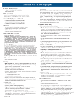
worth noting that this equivalent program does not have to be “materialized” in memory. As before, we consider only rules of the form h : −f (A)Θk for simplicity. We
denote by li1 , . . . , lim the literals belonging to each conji ∈ A, (m > 0). Table 1 summarizes the formulas employed for computing literal occurrences. Note that equivalent
programs in the case of #sum are quite involved, rendering the computation of the
exact values fairly inefficient (many binomial coefficients). Therefore we decided to
approximate the corresponding heuristic value, replacing #sum{A} by #count{A∗ }
where A∗ contains vi different elements, one for each hvi , ti : conji i ∈ A.
As an example, consider a rule of the form h : −#min{A} < k. The equivalent
standard program contains a rule of the type h : −conji , for each vi , 1 ≤ i ≤ n
s.t. vi < k. In this way, h becomes true if one of the conji having vi < k becomes
true, i.e. if the minimum computed by the aggregate is less than k in current answer
set. Thus, the number of occurrences of h in the corresponding standard program are
occ(h) = |{vi : hvi , ti : conji i ∈ A, vi < k}|, while for each literal liz , i.e. the z-th
literal of conji , occ(liz ) = 1 if vi < k, otherwise occ(liz ) = 0.
6 Experimental analysis
We have performed a preliminary experimental analysis on benchmarks with aggregates. In particular, we have considered some domains of the last ASP Competition 13
belonging to the MGS class, together with other benchmarks reported in [6].
All the experiments were performed on a 3GHz PentiumIV equipped with 1GB of
RAM, 2MB of level 2 cache running Debian GNU/Linux. Time measurements have
been done using the time command shipped with the system, counting total CPU time
for the respective process. We report the results in terms of execution time for finding
12
13
Equivalence in general holds only in a stratified setting, which however can serve as an approximation also in non-recursive settings.
http://asparagus.cs.uni-potsdam.de/contest/.
#count{A} < k
#min{A} < k
#max{A} < k
#sum{A} < k
Pk−1 |A|
Pk−1 |A∗ |
k ≤ |A|
k ≤ |A∗ |
i=0
i=0
i
i
occ(h)
|{vi | hvi , ti : conji i ∈ A, vi < k}|
1
1
else
1
else
1 vi < k
occ(lik )
0
0
0
0
else
Pk−1 |A|
Pk−1 |A∗ |
1 vi ≥ k
k ≤ |A|
k ≤ |A∗ |
i=0
i=0
i
i
occ(not lik )
0
0 else
1
else
1
else
#count{A} > k #min{A} > k
#max{A} > k
#sum{A} > k
Pk−1 |A|
Pk−1 |A∗ |
k < |A|
k < |A∗ |
i=0
i=0
i
i
occ(h)
1
|{vi | hvi , ti : conji i ∈ A, vi > k}|
1Pk−1 |A| else
1Pk−1 |A∗ | else
1 vi > k
k < |A|
k < |A∗ |
i=0
i=0
i
i
occ(lik )
0
0 else
1
else
1
else
1 vi ≤ k
occ(not lik )
0
0
0
0 else
Table 1. Occurrence formulas for literals involved in aggregates.
one answer set, if any, within 20 minutes. Results are summarized in Table 2, where the
first column reports the domain name, the second column the total number of instances
considered (in the given domain), the third and fourth columns report the results for the
standard version of DLV ver. of 2007-10-11 in the standard settings and the new system DLVBJA featuring both backjumping and look-back heuristics, and the remaining
columns report the results for CLASP ver. 1.0.4, CMODELS ver. 3.75, SMODELS ver. 2.31
and SMODELS - CC ver 1.08,14 which use LPARSE15 for grounding. The results for the
systems are presented as the mean CPU time of solved instances, along with the number of instances solved within the time limit (in parentheses). Regarding SMODELS - CC,
two results are missing because it can not deal with weight constraint rules.
Domain
BoundedSpanningTree
TowerOfHanoi
WeightedSpanningTree
WeightedLatinSquares
TimeTabling
#I
DLV DLVBJA CLASP CMODELS SMODELS
8
0.13 (8) 0.04 (8) 6.01 (8) 5.69 (8) 101.47 (5)
8
1.16 (8)
1.1 (8) 32.84 (8) 117.32 (7) 259.82 (8)
8
0.04 (8) 0.02 (8) 2.16 (8) 2.31 (8) 28.51 (6)
8 542.23 (6) 140.83 (7) 0.03 (8) 0.34 (8) 326.2 (8)
9
4.49 (9) 0.34 (9) 1.15(9) 0.84 (9) 5.12 (3)
SMODELS - CC
343.35 (8)
154.74 (7)
no enc.
no enc.
96.39 (9)
Table 2. Experimental results: Average execution times (s) (and number of solved instances).
We can see that the first three domains presented are easily solved by both DLV and
DLVBJA , slightly better by the enhanced system, while the remaining solvers show
higher mean CPU time and/or solve less instances. The last two domains further show
the potential of the enhanced system w.r.t. DLV, given it is able to solve more instances
(WeightedLatinSquares domain) in considerably shorter time (DLVBJA is on average
15 times faster on TimeTabling, where the systems solve the same instances, and significantly faster on WeightedLatinSquares, solving also more instances): interestingly,
if compared to the remaining systems, this gain leads DLVBJA to be the best performing solver in 4 domains out of 5 and it performs well in particular in the TimeTabling
domain, while in the WeightedLatinSquares domain its advantage over DLV is just a
step toward the goal of solving all the instances in the domain, as CLASP, CMODELS
and SMODELS.
We are currently working both on improving the performance of the enhanced system (by developing further optimizations both by enhancing the implementation of the
reason calculus and by considering different “equivalent programs”, and, thus, different
VSIDS initializations) and by including new benchmarks. Regarding this last point, we
want to mention one more result on the comparison between DLVBJA and DLV (other
solvers are running): on the Seating benchmarks from [6], DLVBJA solves one more
instance (820 instead of 819 out of 910), with mean CPU time 1.24 and 31.46 seconds
for DLVBJA and DLV, respectively.
14
15
http://www.cs.uni-potsdam.de/clasp,
http://www.cs.utexas.edu/users/tag/cmodels.html,
http://www.tcs.hut.fi/Software/smodels and http://www.nku.edu/ wardj1/Research/smodels cc.html,
respectively.
http://www.tcs.hut.fi/Software/lparse.
7 Conclusion
In this paper we have described look-back techniques for the evaluation of aggregates,
which represent one of the most relevant improvements both ASP language and systems. In particular the main contributions are: (i) an extension of the reason calculus
defined in [8]; and, (ii) an enhanced version of the heuristic presented in [9] that explicitly takes into account the presence of aggregates. Moreover, we have implemented
the proposed techniques in a prototypical version of the DLV system and performed
a set of preliminary benchmarks which indicate performance benefits of the enhanced
system.
References
1. Gelfond, M., Lifschitz, V.: Classical Negation in Logic Programs and Disjunctive Databases.
NGC 9 (1991) 365–385
2. Pelov, N., Denecker, M., Bruynooghe, M.: Well-founded and Stable Semantics of Logic
Programs with Aggregates. TPLP 7(3) (2007) 301–353
3. Son, T.C., Pontelli, E.: A Constructive Semantic Characterization of Aggregates in ASP.
TPLP 7 (2007) 355–375
4. Faber, W., Leone, N., Pfeifer, G.: Recursive aggregates in disjunctive logic programs: Semantics and complexity. In: JELIA 2004. LNCS 3229, (2004) 200–212
5. Simons, P., Niemel¨a, I., Soininen, T.: Extending and Implementing the Stable Model Semantics. AI 138 (2002) 181–234
6. Dell’Armi, T., Faber, W., Ielpa, G., Leone, N., Pfeifer, G.: Aggregate Functions in DLV. In:
ASP’03, Messina, Italy (2003) 274–288 Online at http://CEUR-WS.org/Vol-78/.
7. Gebser, M., Kaufmann, B., Neumann, A., Schaub, T.: Conflict-driven answer set solving.
In: IJCAI 2007,(2007) 386–392
8. Ricca, F., Faber, W., Leone, N.: A Backjumping Technique for Disjunctive Logic Programming. AI Communications 19(2) (2006) 155–172
9. Faber, W., Leone, N., Maratea, M., Ricca, F.: Experimenting with Look-Back Heuristics for
Hard ASP Programs. In: LPNMR’07. LNCS 4483, (2007) 110–122
10. Baral, C.: Knowledge Representation, Reasoning and Declarative Problem Solving. CUP
(2003)
11. Gaschnig, J.: Performance measurement and analysis of certain search algorithms. PhD
thesis, CMU (1979) Tech. Report CMU-CS-79-124.
12. Prosser, P.: Hybrid Algorithms for the Constraint Satisfaction Problem. Computational
Intelligence 9 (1993) 268–299
13. Faber, W.: Enhancing Efficiency and Expressiveness in Answer Set Programming Systems.
PhD thesis, TU Wien (2002)
14. Moskewicz, M.W., Madigan, C.F., Zhao, Y., Zhang, L., Malik, S.: Chaff: Engineering an
Efficient SAT Solver. In: DAC 2001 (2001) 530–535