
Gary G. Matthews
Cellular Physiology
of Nerve and Muscle
Gary G. Matthews
Department of Neurobiology
State University of New York
at Stony Brook
Fourth
Edition
CELLULAR PHYSIOLOGY OF NER VE AND MUSCLE
Cellular Physiology
of Nerve and Muscle
Gary G. Matthews
Department of Neurobiology
State University of New York
at Stony Brook
Fourth
Edition
© 2003 by Blackwell Science Ltd
a Blackwell Publishing company
350 Main Street, Malden, MA 02148-5018, USA
108 Cowley Road, Oxford OX4 1JF, UK
550 Swanston Street, Carlton, Victoria 3053, Australia
Kurfürstendamm 57, 10707 Berlin, Germany
The right of Gary G. Matthews to be identified as the Author of this Work has been asserted in
accordance with the UK Copyright, Designs, and Patents Act 1988.
All rights reserved. No part of this publication may be reproduced, stored in a retrieval system,
or transmitted, in any form or by any means, electronic, mechanical, photocopying, recording
or otherwise, except as permitted by the UK Copyright, Designs, and Patents Act 1988,
without the prior permission of the publisher.
First edition published 1986 by Blackwell Scientific Publications
Second edition published 1991
Third edition published 1998 by Blackwell Science, Inc.
Fourth edition published 2003 by Blackwell Science Ltd
Library of Congress Cataloging-in-Publication Data
Matthews, Gary G., 1949–
Cellular physiology of nerve and muscle / Gary G. Matthews. 4th ed.
p. ; cm.
Includes bibliographical references and index.
ISBN 1-40510-330-2
1. Neurons. 2. Muscle cells. 3. Nerves Cytology. 4. Muscles Cytology.
[DNLM: 1. Membrane Potentials physiology. 2. Neurons physiology.
3. Muscles cytology. 4. Muscles physiology. WL 102.5 M439c 2003]
I. Title.
QP363 .M38 2003
573.8′36 dc21
2002003951
A catalogue record for this title is available from the British Library.
Set in 11/12.5pt Octavian
by Graphicraft Ltd, Hong Kong
Printed and bound in the United Kingdom
by TJ International, Padstow, Cornwall
For further information on
Blackwell Publishing, visit our website:
http://www.blackwellpublishing.com
Contents
Preface ix
Acknowledgments x
Part I: Origin of Electrical Membrane
Potential 1
1 Introduction to Electrical Signaling in the Nervous
System 3
The Patellar Reflex as a Model for Neural Function 3
The Cellular Organization of Neurons 4
Electrical Signals in Neurons 5
Transmission between Neurons 6
2 Composition of Intracellular and Extracellular Fluids 9
Intracellular and Extracellular Fluids 10
The Structure of the Plasma Membrane 11
Summary 16
3 Maintenance of Cell Volume 17
Molarity, Molality, and Diffusion of Water 17
Osmotic Balance and Cell Volume 20
Answers to the Problem of Osmotic Balance 21
Tonicity 24
Time-course of Volume Changes 24
Summary 25
4 Membrane Potential: Ionic Equilibrium 26
Diffusion Potential 26
Equilibrium Potential 28
The Nernst Equation 28
The Principle of Electrical Neutrality 30
The Cell Membrane as an Electrical Capacitor 31
Incorporating Osmotic Balance 32
Donnan Equilibrium 33
A Model Cell that Looks Like a Real Animal Cell 35
vi
Contents
The Sodium Pump 37
Summary 38
5 Membrane Potential: Ionic Steady State 40
Equilibrium Potentials for Sodium, Potassium, and Chloride 40
Ion Channels in the Plasma Membrane 41
Membrane Potential and Ionic Permeability 41
The Goldman Equation 45
Ionic Steady State 47
The Chloride Pump 48
Electrical Current and the Movement of Ions Across Membranes 48
Factors Affecting Ion Current Across a Cell Membrane 50
Membrane Permeability vs. Membrane Conductance 50
Behavior of Single Ion Channels 52
Summary 54
Part II: Cellular Physiology of Nerve Cells 55
6 Generation of Nerve Action Potential 57
The Action Potential 57
Ionic Permeability and Membrane Potential 57
Measuring the Long-distance Signal in Neurons 57
Characteristics of the Action Potential 59
Initiation and Propagation of Action Potentials 60
Changes in Relative Sodium Permeability During an
Action Potential 63
Voltage-dependent Sodium Channels of the Neuron
Membrane 64
Repolarization 66
The Refractory Period 69
Propagation of an Action Potential Along a Nerve Fiber 71
Factors Affecting the Speed of Action Potential Propagation 73
Molecular Properties of the Voltage-sensitive Sodium Channel 75
Molecular Properties of Voltage-dependent Potassium
Channels 78
Calcium-dependent Action Potentials 78
Summary 83
7 The Action Potential: Voltage-clamp Experiments 85
The Voltage Clamp 85
Measuring Changes in Membrane Ionic Conductance Using the
Voltage Clamp 87
The Squid Giant Axon 90
Ionic Currents Across an Axon Membrane Under
Voltage Clamp 90
Contents vii
The Gated Ion Channel Model 94
Membrane Potential and Peak Ionic Conductance 94
Kinetics of the Change in Ionic Conductance Following a
Step Depolarization 97
Sodium Inactivation 101
The Temporal Behavior of Sodium and Potassium
Conductance 105
Gating Currents 107
Summary 108
8 Synaptic Transmission at the Neuromuscular
Junction 110
Chemical and Electrical Synapses 110
The Neuromuscular Junction as a Model Chemical Synapse 111
Transmission at a Chemical Synapse 111
Presynaptic Action Potential and Acetylcholine Release 111
Effect of Acetylcholine on the Muscle Cell 113
Neurotransmitter Release 115
The Vesicle Hypothesis of Quantal Transmitter Release 117
Mechanism of Vesicle Fusion 121
Recycling of Vesicle Membrane 123
Inactivation of Released Acetylcholine 124
Recording the Electrical Current Flowing Through a Single
Acetylcholine-activated Ion Channel 124
Molecular Properties of the Acetylcholine-activated
Channel 127
Summary 129
9 Synaptic Transmission in the Central Nervous
System 130
Excitatory and Inhibitory Synapses 130
Excitatory Synaptic Transmission Between Neurons 131
Temporal and Spatial Summation of Synaptic Potentials 131
Some Possible Excitatory Neurotransmitters 133
Conductance-decrease Excitatory Postsynaptic Potentials 136
Inhibitory Synaptic Transmission 137
The Synapse between Sensory Neurons and Antagonist Motor
Neurons in the Patellar Reflex 137
Characteristics of Inhibitory Synaptic Transmission 138
Mechanism of Inhibition in the Postsynaptic Membrane 139
Some Possible Inhibitory Neurotransmitters 141
The Family of Neurotransmitter-gated Ion Channels 143
Neuronal Integration 144
Indirect Actions of Neurotransmitters 146
Presynaptic Inhibition and Facilitation 149
Synaptic Plasticity 152
viii Contents
Short-term Changes in Synaptic Strength 152
Long-term Changes in Synaptic Strength 154
Summary 158
Part III: Cellular Physiology of Muscle
Cells 161
10 Excitation–Contraction Coupling in Skeletal Muscle 163
The Three Types of Muscle 163
Structure of Skeletal Muscle 165
Changes in Striation Pattern on Contraction 165
Molecular Composition of Filaments 167
Interaction between Myosin and Actin 169
Regulation of Contraction 172
The Sarcoplasmic Reticulum 173
The Transverse Tubule System 174
Summary 176
11 Neural Control of Muscle Contraction 177
The Motor Unit 177
The Mechanics of Contraction 178
The Relationship Between Isometric Tension and
Muscle Length 180
Control of Muscle Tension by the Nervous System 182
Recruitment of Motor Neurons 182
Fast and Slow Muscle Fibers 184
Temporal Summation of Contractions Within a Single Motor
Unit 184
Asynchronous Activation of Motor Units During Maintained
Contraction 185
Summary 187
12 Cardiac Muscle: The Autonomic Nervous System 188
Autonomic Control of the Heart 191
The Pattern of Cardiac Contraction 191
Coordination of Contraction Across Cardiac Muscle Fibers 193
Generation of Rhythmic Contractions 196
The Cardiac Action Potential 196
The Pacemaker Potential 199
Actions of Acetylcholine and Norepinephrine on Cardiac
Muscle Cells 201
Summary 206
Appendix A: Derivation of the Nernst Equation 208
Appendix B: Derivation of the Goldman Equation 212
Appendix C: Electrical Properties of Cells 216
Suggested Readings 225
Index 230
Preface to the
Fourth Edition
The fourth edition of Cellular Physiology of Nerve and Muscle incorporates
new material in several areas. An opening chapter has been added to introduce
the basic characteristics of electrical signaling in the nervous system and to
set the stage for the detailed topics covered in Part I. The coverage of
synaptic transmission has been expanded to include synaptic plasticity, a topic
requested by students and instructors alike. A new appendix has been included
that covers the basic electrical properties of cells in greater detail for those who
want a more quantitative treatment of this material.
Perhaps the most salient change is the artwork, with many new figures in
this edition. As in previous editions, the goal of each figure is to clarify a single
point of discussion, but I hope the new illustrations will also be more visually
striking, while retaining their teaching purpose.
Students should also note that animations are available for selected figures, as indicated in the figure captions. The animations are available at
www.blackwellscience.com by following the link for my general neurobiology
text: Neurobiology: Molecules, Cells, and Systems.
Despite the numerous improvements in the fourth edition, the underlying
core of the book remains the same: a step-by-step presentation of the physical
and chemical principles necessary to understand electrical signaling in cells.
This material is necessarily quantitative. However, I am confident that the
approach taken here will allow students to arrive at a sophisticated understanding of how cells generate electrical signals and use them to communicate.
G.G.M.
Acknowledgments
Special thanks go to the following reviewers who offered their expert advice
about the planned changes for the fourth edition. Their input was of great
value.
Klaus W. Beyenbach, Cornell University
Scott Chandler, UCLA
Jon Johnson, University of Pittsburgh
Robert Paul Malchow, University of Illinois at Chicago
Stephen D. Meriney, University of Pittsburgh
Origin of Electrical
Membrane Potential
This book is about the physiological characteristics of nerve and muscle cells.
As we shall see, the ability of these cells to generate and conduct electricity is
fundamental to their functioning. Thus, to understand the physiology of nerve
and muscle, we must understand the basic physical and chemical principles
underlying the electrical behavior of cells.
Because an understanding of how electrical voltages and currents arise
in cells is central to our goals in this book, Part I is devoted to this task. The
discussion begins with the differences in composition of the fluids inside and
outside cells and culminates in a quantitative understanding of how ionic
gradients across the cell membrane give rise to a transmembrane voltage. This
quantitative description sets the stage for the specific descriptions of nerve and
muscle cells in Parts II and III of the book and is central to understanding how
the nervous system functions as a transmitter of electrical signals.
I
part
Introduction to
Electrical Signaling
in the Nervous System
1
The Patellar Reflex as a Model for Neural Function
To set the stage for discussing the generation and transmission of signals in the
nervous system, it will be useful to describe the characteristics of those signals
using a simple example: the patellar reflex, also known as the knee-jerk reflex.
Figure 1-1 shows the neural circuitry underlying the patellar reflex. Tapping
the patellar tendon, which connects the knee cap (patella) to the bones of the
lower leg, pulls the knee cap down and stretches the quadriceps muscle at the
front of the thigh. Specialized nerve cells (sensory neurons) sense the stretch of
the muscle and send a signal that travels along the thin fibers of the sensory
Thigh muscle
(quadriceps)
Sensory
fiber
Afferent
(incoming)
signal
Sensory
neuron
Knee cap
(patella)
Patellar
tendon
Motor
nerve
Leg bones fiber
Spinal cord
Efferent
(outgoing)
signal
Motor
neuron
Figure 1-1 A schematic representation of the patellar reflex. The sensory neuron is activated by
stretching the thigh muscle. The incoming (afferent) signal is carried to the spinal cord along the nerve
fiber of the sensory neuron. In the spinal cord, the sensory neuron activates motor neurons, which in
turn send outgoing (efferent) signals along the nerve back to the thigh muscle, causing it to contract.
4
Introduction to Electrical Signaling in the Nervous System
neurons from the muscle to the spinal cord. In the spinal cord, the sensory
signal is received by other neurons, called motor neurons. The motor neurons
send nerve fibers back to the quadriceps muscle and command the muscle to
contract, which causes the knee joint to extend.
The reflex loop exemplified by the patellar reflex embodies in a particularly
simple way all of the general features that characterize the operation of the
nervous system. A sensory stimulus (muscle stretch) is detected, the signal
is transmitted rapidly over long distance (to and from the spinal cord), and
the information is focally and specifically directed to appropriate targets (the
quadriceps motor neurons, in the case of the sensory neurons, and the quadriceps muscle cells, in the case of the motor neurons). The sensory pathway,
which carries information into the nervous system, is called the afferent
pathway, and the motor output constitutes the efferent pathway. Much of the
nervous system is devoted to processing afferent sensory information and then
making the proper connections with efferent pathways to ensure that an appropriate response occurs. In the case of the patellar reflex, the reflex loop ensures
that passive stretch of the muscle will be automatically opposed by an active
contraction, so that muscle length remains constant.
The Cellular Organization of Neurons
Neurons are structurally complex cells, with long fibrous extensions that
are specialized to receive and transmit information. This complexity can be
appreciated by examining the structure of a motor neuron, shown schematically in Figure 1-2a. The cell body, or soma, of the motor neuron where
the nucleus resides is only about 20–30 µm in diameter in the case of
motor neurons involved in the patellar reflex. The soma is only a small part
of the neuron, however, and it gives rise to a tangle of profusely branching
processes called dendrites, which can spread out for several millimeters within
the spinal cord. The dendrites are specialized to receive signals passed along
as the result of the activity of other neurons, such as the sensory neurons of
the patellar reflex, and to funnel those signals to the soma. The soma also
gives rise to a thin fiber, the axon, that is specialized to transmit signals
over long distances. In the case of the motor neuron in the patellar reflex, the
axon extends all the way from the spinal cord to the quadriceps muscle, a
distance of approximately 1 meter. As shown in Figure 1-2b, the sensory
neuron of the patellar reflex is structurally simpler than the motor neuron.
Its soma, which is located just outside the spinal cord in the dorsal root ganglion, gives rise to only a single nerve fiber, the axon. The axon splits into two
branches shortly after it exits the dorsal root ganglion: one branch extends
away from the spinal cord to contact the muscle cells of the quadriceps muscle,
and the other branch passes into the spinal cord to contact the quadriceps
motor neurons. The axon of the sensory neuron carries the signal generated
by muscle stretch from the muscle into the spinal cord. Because the sensory
Electrical Signals in Neurons 5
(a) Motor neuron within spinal cord
Dendrites
Soma
Axon
To muscle
20µm
Glial cells
(b) Sensory neuron just outside spinal cord
Soma
From muscle
Axon
To spinal cord
Figure 1-2 Structures of
single neurons involved in
the patellar reflex.
neuron receives its input signal from the sensory stimulus (muscle stretch) at
the peripheral end of the axon instead of from other neurons, it lacks the dendrites seen in the motor neuron.
Electrical Signals in Neurons
To transmit information rapidly over long distances, neurons produce active
electrical signals, which travel along the axons that make up the transmission
paths. The electrical signal arises from changes in the electrical voltage difference across the cell membrane, which is called the membrane potential.
6
Introduction to Electrical Signaling in the Nervous System
Although this transmembrane voltage is small typically less than a tenth of a
volt it is central to the functioning of the nervous system. Information is
transmitted and processed by neurons by means of changes in the membrane
potential.
What does the electrical signal that carries the message along the sensory
nerve fiber in the patellar reflex look like? To answer this question, we must
measure the membrane potential of the sensory neuron by placing an ultrafine
voltage-sensing probe, called an intracellular microelectrode, inside the sensory nerve fiber, as illustrated in Figure 1-3. A voltmeter is connected to measure the voltage difference between the tip of the intracellular microelectrode
(point a in the figure) and a reference point in the extracellular space (point b).
When the microelectrode is located outside the sensory neuron, both points
a and b are in the extracellular space, and the voltmeter therefore records no
voltage difference (Figure 1-3b). When the tip of the probe is inserted inside
the sensory neuron, however, the voltmeter measures an electrical potential
between points a and b, representing the voltage difference between the
inside and the outside of the neuron that is, the membrane potential of the
neuron. As shown in Figure 1-3b, the inside of the sensory nerve fiber is negative with respect to the outside by about seventy-thousandths of a volt (1 millivolt, abbreviated mV, equals one-thousandth of a volt). Because the potential
outside the cell is our reference point and the inside is negative with respect
to the outside, the membrane potential is represented as a negative number,
i.e., −70 mV.
As long as the sensory neuron is not stimulated by stretching the muscle, the
membrane potential remains constant at this resting value. For this reason, the
unstimulated membrane potential is known as the resting potential of the cell.
When the muscle is stretched, however, the membrane potential of the sensory
neuron undergoes a dramatic change, as shown in Figure 1-3b. After a delay
that depends on the distance of the recording site from the muscle, the membrane potential suddenly moves in the positive direction, transiently reverses
sign for a brief period, and then returns to the resting negative level. This transient jump in membrane potential is the action potential the long-distance
signal that carries information in the nervous system.
Transmission between Neurons
What happens when the action potential reaches the end of the neuron, and the
signal must be transmitted to the next cell? In the patellar reflex, signals are
relayed from one cell to another at two locations: from the sensory neuron to the
motor neuron in the spinal cord, and from the motor neuron to the muscle cells
in the quadriceps muscle. The point of contact where signals are transmitted
from one neuron to another is called a synapse. In the patellar reflex, both the
synapse between the sensory neuron and the motor neuron and the synapse
between the motor neuron and the muscle cells are chemical synapses, in which
Transmission between Neurons 7
Sensory neuron
(a)
Muscle cell
b
Voltage-sensing
microelectrode
Sensory nerve fiber
Outside
Inside
a
(b)
Membrane potential (mV)
+50
Probe penetrates
fiber
Probe a outside
fiber
Action potential
0
–50
Resting
membrane
potential
–100
Stretch muscle
Time
an action potential in the input cell (the presynaptic cell) causes it to release
a chemical substance, called a neurotransmitter. The molecules of neurotransmitter then diffuse through the extracellular space and change the
membrane potential of the target cell (the postsynaptic cell). The change in
membrane potential of the target then affects the firing of action potentials
Figure 1-3 Recording the
action potential in the nerve
fiber of the sensory neuron
in the patellar stretch reflex.
(a) A diagram of the
recording configuration.
A tiny microelectrode is
inserted into the sensory
nerve fiber, and a voltmeter
is connected to measure
the voltage difference (E)
between the inside (a)
and the outside (b) of the
nerve fiber. (b) When the
microelectrode penetrates
the fiber, the resting
membrane potential of the
nerve fiber is measured.
When the sensory neuron is
activated by stretching the
muscle, an action potential
occurs and is recorded as a
rapid shift in the recorded
membrane potential of the
sensory nerve fiber.
8
Introduction to Electrical Signaling in the Nervous System
Presynaptic action potential
Depolarization of synaptic terminal
Figure 1-4 Chemical
transmission mediates
synaptic communication
between cells in the patellar
reflex. The flow diagram
shows the sequence of
events involved in the
release of chemical
neurotransmitter from
the synaptic terminal.
Release of chemical
neurotransmitter
Neurotransmitter changes electrical
potential of postsynaptic cell
by the postsynaptic cell. This sequence of events during synaptic transmission
is summarized in Figure 1-4.
Because signaling both within and between cells in the nervous system
involves changes in the membrane potential, the brain is essentially an
electrochemical organ. Therefore, to understand how the brain functions, we
must first understand the electrochemical mechanisms that give rise to a
transmembrane voltage in cells. The remaining chapters in Part I are devoted
to the task of developing the basic chemical and physical principles required to
comprehend how cells communicate in the nervous system. In Part II, we will
then consider how these electrochemical principles are exploited in the nervous
system for both long-distance communication via action potentials and local
communication at synapses.
Composition of
Intracellular and
Extracellular Fluids
When we think of biological molecules, we normally think of all the special
molecules that are unique to living organisms, such as proteins and nucleic
acids: enzymes, DNA, RNA, and so on. These are the substances that allow
life to occur and that give living things their special characteristics. Yet, if we
were to dissociate a human body into its component molecules and sort them
by type, we would find that these special molecules are only a small minority of
the total. Of all the molecules in a human body, only about 0.25% fall within
the category of these special biological molecules. Most of the molecules are
far more ordinary. In fact, the most common molecule in the body is water.
Excluding nonessential body fat, water makes up about 75% of the weight of a
human body. Because water is a comparatively light molecule, especially when
compared with massive protein molecules, this 75% of body weight translates
into a staggering number of molecules of water. Thus, water molecules account
for about 99% of all molecules in the body. The remaining 0.75% consists of
other simple inorganic substances, mostly sodium, potassium, and chloride
ions. In the first part of this book we will be concerned in large part with the
mundane majority of molecules, the 99.75% made up of water and inorganic
ions.
Why should we study these mundane molecules? Many enzymatic reactions
involving the more glamorous organic molecules require the participation
of inorganic cofactors, and most biochemical reactions within cells occur
among substances that are dissolved in water. Nevertheless, most inorganic
molecules in the body never participate in any biochemical reactions. In spite of
this, a sufficient reason to study these inorganic substances is that cells could
not exist and life as we know it would not be possible if cells did not possess
mechanisms to control the distribution of water and ions across their membranes. The purpose of this chapter is to see why that is true and to understand
the physical principles that underlie the ability of cells to maintain their
integrity in a hostile physicochemical environment.
2
10
Composition of Intracellular and Extracellular Fluids
Intracellular and Extracellular Fluids
The water in the body can be divided into two compartments: intracellular and
extracellular fluid. About 55% of the water is inside cells, and the remainder is
outside. The extracellular fluid, or ECF, can in turn be subdivided into plasma,
lymphatic fluid, and interstitial fluid, but for now we can lump all the ECF
together into one compartment. Similarly there are subcompartments within
cells, but it will suffice for now to treat cells as uniform bags of fluid. The wall
that separates the intracellular and extracellular fluid compartments is the
outer cell membrane, also called the plasma membrane of the cell.
Both organic and inorganic substances are dissolved in the intracellular and
extracellular water, but the compositions of the two fluid compartments differ.
Table 2-1 shows simplified compositions of ECF and intracellular fluid (ICF)
for a typical mammalian cell. The compositions shown in the table are simplified by including only those substances that are important in governing the
basic osmotic and electrical properties of cells. Many other kinds of inorganic
and organic solutes beyond those shown in the table are present in both the
ECF and ICF, and many of them have important physiological roles in other
contexts. For the present, however, they can be ignored.
The principal cation (positively charged ion) outside the cell is sodium,
although there is also a small amount of potassium, which will be important to
consider when we discuss the origin of the membrane potential of cells. Inside
cells, the situation is reversed, with a small amount of sodium and potassium
being the principal cation. Negatively charged chloride ions, which are present
at a high concentration in ECF, are relatively scarce in ICF. The major anion
(negatively charged ion) inside cells is actually a class of molecules that bear
a net negative charge. These intracellular anions, which we will abbreviate
A−, include protein molecules, acidic amino acids like aspartate and glutamate, and inorganic ions like sulfate and phosphate. For the purposes of this
Table 2-1 Simplified compositions of intracellular and extracellular
fluids for a typical mammalian cell.
K+
Na+
Cl−
A−
H2O
Internal
concentration
(mM )
External
concentration
(mM )
Can it
cross plasma
membrane?
125
12
5
108
55,000
5
120
125
0
55,000
Y
N*
Y
N
Y
Membrane potential = −60 to −100 mV
*As we will see in Chapter 3, this “No” is not as simple as it first appears.
The Structure of the Plasma Membrane 11
book, the anions of this class outside cells can be ignored, and we will simplify
the situation by assuming that the sole extracellular anion is chloride.
It will also be important to consider the concentration of water on the two
sides of the membrane, which is also shown in Table 2-1. It may seem odd to
speak of the “concentration” of the solvent in ECF and ICF. However, as we
shall see when we consider the maintenance of cell volume, the concentration of
water must be the same inside and outside the cell, or water will move across
the membrane and cell volume will change.
Another important consideration will be whether a particular substance can
cross the plasma membrane that is, whether the membrane is permeable to
that substance. The plasma membrane is permeable to water, potassium, and
chloride, but is effectively impermeable to sodium (however, we will reconsider
the sodium permeability later). Of course, if the membrane is to do its job properly, it must keep the organic anions inside the cell; otherwise, all of a cell’s
essential biochemical machinery would simply diffuse away into the ECF.
Thus, the membrane is impermeable to A−.
As described in Chapter 1, there is an electrical voltage across the plasma
membrane, with the inside of the cell being more negative than the outside. The
voltage difference is usually about 60–100 millivolts (mV), and is referred to as
the membrane potential of the cell. By convention, the potential outside the cell
is called zero; therefore, the typical value of the membrane potential (abbreviated Em) is −60 to −100 mV, as shown in Table 2-1. A major concern of the first
section of this book will be the origin of this electrical membrane potential.
In later sections, we will discuss how the membrane potential influences the
movement of charged particles across the cell membrane and how the electrical
energy stored in the membrane potential can be tapped to generate signals that
can be passed from one cell to another in the nervous system.
The Structure of the Plasma Membrane
Before we consider the mechanisms that allow cells to maintain the differences
in ECF and ICF shown in Table 2-1, it will be helpful to look at the structure of
the outer membrane of the cell, the plasma membrane. The control mechanisms
responsible for the differences between ICF and ECF reside within the plasma
membrane, which forms the barrier between the intracellular and extracellular
compartments.
It has long been known that the contents of a cell will leak out if the cell is
damaged by being poked or prodded with a glass probe. Also, some dyes will
not enter cells when dissolved in the ECF, and the same dyes will not leak out
when injected inside cells. These observations, first made in the nineteenth
century, led to the idea that there is a selectively permeable barrier the plasma
membrane separating the intracellular and extracellular fluids.
The first systematic observations of the kinds of molecules that would enter
cells and the kinds that were excluded were made by Overton in the early part
12
Composition of Intracellular and Extracellular Fluids
of the twentieth century. He found that, in general, substances that are highly
soluble in lipids enter cells more easily than substances that are less soluble in
lipids. Lipids are molecules that are not soluble in water or other polar solvents,
but are soluble in oil or other nonpolar solvents. Thus, Overton suggested that
the plasma membrane of a cell is made of lipids and that substances can cross
the membrane if they can dissolve in the membrane lipids.
There were some exceptions to the general lipid solubility rule. Electrically
charged substances, like potassium and chloride ions, are almost totally insoluble in lipids, yet they manage to cross the plasma membrane. Other substances, such as urea, entered cells more easily than expected from their lipid
solubility alone. To take account of these exceptions, Overton suggested that
the lipid membrane is shot through with tiny holes or pores that allow highly
water soluble (hydrophilic) substances, such as ions, to cross the membrane.
Only hydrophilic substances that are small enough to fit through these small
aqueous pores can cross the membrane. Larger molecules like proteins and
amino acids cannot fit through the pores and thus cannot cross the membrane
without the help of special transport mechanisms.
The molecules of the lipid skin of cell membranes appear to be arranged in a
layer only two molecules thick. Evidence for this arrangement was obtained
from experiments in which the lipids were chemically extracted from the
plasma membranes of cells and spread out on a trough of water in such a way
that they formed a film only one molecule thick. When the area of this monolayer “oil slick” was measured, it was found to be about twice the total surface
area of the intact cells from which the lipids were obtained. This suggests that
the membrane of the intact cells was two molecules thick. Such a membrane is
called a lipid bilayer membrane.
The bilayer arrangement of the cell membrane makes chemical sense
when we consider the characteristics of the particular lipid molecules found in
the plasma membrane. The cell lipids are largely phospholipids, which are
molecules that have both a polar region that is hydrophilic and a nonpolar
region that is hydrophobic. When surrounded by water, these lipid molecules
tend to aggregate, with the hydrophilic regions oriented outward toward
the surrounding water and the hydrophobic regions pointed inward toward
each other. When spread out in a sheet with water on each side of the sheet, the
phospholipids can maintain their preferred state by forming a bimolecular
sandwich, with the hydrophilic parts on the outside toward the water, and
the hydrophobic parts in the middle, pointed toward each other. This bilayer
model for the cell plasma membrane is illustrated in Figure 2-1.
Figure 2-1 also shows another important characteristic of cell membranes.
They contain not only lipid molecules but also protein molecules. Some proteins are attached to the inner or outer surface of the cell membrane, and others
penetrate all the way through the membrane so that they form a bridge from
one side to the other. Some of these transmembrane proteins form the aqueous
pores, or channels, that allow ions and other small hydrophilic molecules to
cross the membrane. If we separate membranes from the rest of the cell and
The Structure of the Plasma Membrane 13
Proteins
Ion channels
(proteins)
Plasma
membrane
Transmembrane
protein
Phospholipid
molecule
Aqueous
pore
Cross-section
of channel
Figure 2-1 A schematic diagram of a section of the plasma membrane. The backbone of the
membrane is a sheet of lipid molecules two molecules thick. Inserted into this sheet are various types
of protein molecules. Some protein molecules extend all the way across the sheet, from the inner to
the outer face. These transmembrane proteins sometimes form aqueous pores or channels through
which small hydrophilic molecules, such as ions, can cross the membrane. The diagram shows two
such channels; one is cut in cross-section to reveal the interior of the pore.
analyze their composition, we find that, by weight, only about one-third of the
membrane material is lipid; most of the rest is protein. Thus, the lipids form the
backbone of the membrane, but proteins are an important part of the picture.
We will see later that the proteins are very important in controlling the movement of substances, particularly ions, across the cell membrane.
We can get an idea of the importance of membrane proteins for life by examining how much of the entire genome of a simple organism is taken up by genes
encoding membrane proteins. One of the smallest genomes of any free-living
organism is that of Mycoplasma genitalium, a microbe whose genome can be
regarded as close to the minimum required for an independent, cellular life
form. The DNA of M. genitalium has been completely sequenced, revealing a
total of 482 individual genes. Of this total, 140 genes, or about 30%, code for
membrane proteins. Thus, M. genitalium expends a large fraction of its total
available DNA for the membrane proteins that sit at the interface between the
microbe and its external environment. This points out the central role of these
proteins in the maintenance of cellular life.
Anatomical evidence also supports the model shown in Figure 2-1. The
cell membrane is much too thin to be seen with the light microscope. In fact, it
is almost too thin to be seen with the electron microscope. However, with an
electron microscope it is possible to see at the outer boundary of a cell a threelayered (trilaminar) profile like a railroad track, with a light central region separating two darker bands. Figure 2-2 is an example of an electron micrograph
14
Composition of Intracellular and Extracellular Fluids
Figure 2-2 High-power
electron micrograph of the
plasma membranes of two
neighboring cells. Note the
two dark bands separated
by a light region at the outer
surface of each cell. The
two cells are nerve cells
from the brain, and the
point of close contact
between them is a synapse,
the point of information
transfer in the nervous
system. Note also the
membrane-bound
intracellular structures
(labeled SV), called synaptic
vesicles, inside one of
the cells; the vesicle
membranes also have the
trilaminar profile seen in the
plasma membranes. We will
learn more about synaptic
vesicles and synapses in
Chapters 8 and 9. (Courtesy
of A. L. deBlas of the
University of Connecticut.)
showing the plasma membranes of two cells lying in close contact. The interpretation of the trilaminar profile is that the two dark bands represent the polar
heads of the membrane phospholipids and protein molecules on the inner and
outer surfaces of the membrane and that the lighter region between the two
dark bands represents the nonpolar tails of the lipid molecules. The total thickness of the sandwich is about 7.5 nm. The lighter-colored “fuzz” surrounding
the trilaminar profiles of the two cell membranes in Figure 2-2 consists in part
of portions of membrane-associated protein molecules extending out into the
intracellular and extracellular spaces. The two cells shown in Figure 2-2 are
nerve cells (neurons) in the brain, and the region of close contact is a specialized
junction, called a synapse, where electrical activity is relayed from one nerve
cell to another. The synapse is the basic mechanism of information transfer
in the brain, and one of our major goals in this book is to understand how
synapses work.
By using a special form of microscopy called freeze-fracture electron
microscopy, it is possible to visualize more clearly the protein molecules that
are embedded in the plasma membrane. A schematic representation of the
freeze-fracture technique is shown in Figure 2-3. A small sample of the tissue
to be examined is frozen in liquid nitrogen, and then a thin sliver of the frozen
tissue is shaved off with a sharp knife. Because the tissue is frozen, however, the sliver is not so much sliced off as broken off from the sample. In some
cases, like that shown in Figure 2-3, the line of fracture runs between the two
lipid layers of the membrane bilayer, leaving holes where protein molecules
are ripped out of the lipid monolayer and protrusions where membrane
SV
0.1 µm
The Structure of the Plasma Membrane 15
Pho
Figure 2-3 Schematic illustration of the freeze-fracture procedure for electron microscopy. When a
fracture line runs between the two lipid layers of the plasma membrane, some membrane proteins
stay with one monolayer, others with the other layer. When the fractured surface is then examined
with the electron microscope, the remaining proteins appear as protruding bumps in the surface.
proteins are ripped out of the opposing monolayer and come along with the
shaved sliver. An example of such a freeze-fracture sample viewed through
the electron microscope is shown in Figure 2-4. The membrane proteins
appear as small bumps in the otherwise smooth surface of the plasma membrane, like grains of sand sprinkled on a freshly painted surface. In the discussion of the transmission of signals at synapses in Chapter 8, we will see other
examples of freeze-fracture electron micrographs and see how they can
provide important evidence about the physiological functioning of cells.
16
Composition of Intracellular and Extracellular Fluids
Figure 2-4 Example of a
fractured membrane
surface containing protein
molecules, viewed through
the electron microscope.
The membrane surface
shown is that of the
presynaptic nerve terminal
at the nerve–muscle
junction, which will be
discussed in detail in
Chapter 8. The protein
molecules are the small
bumps scattered about on
the planar surface of the
membrane. (Reproduced
from C.-P. Ko, Regeneration
of the active zone at the frog
neuromuscular junction.
Journal of Cell Biology
1984;98:1685–1695; by
copyright permission of
the Rockefeller University
Press.)
Summary
The most common molecules in the body are water and simple inorganic
molecules mainly sodium, potassium, and chloride ions. The water in the
body can be divided into two compartments: the intracellular and extracellular
fluids. The barrier between those two compartments is the plasma membrane
of the cell, which is a phospholipid bilayer with protein molecules inserted into
it. The extracellular fluid is high in sodium and chloride, but low in potassium,
while the intracellular fluid is low in sodium and chloride, but high in potassium. This difference is maintained and regulated by control mechanisms
residing in the plasma membrane, which acts as a selectively permeable barrier
permitting some substances to cross but excluding others.
Maintenance of
Cell Volume
3
At an early stage of evolution, before the development of cells, life might well
have been nothing more than a loose confederation of enzyme systems and selfreplicating molecules. A major problem faced by such acellular systems must
have been how to keep their constituent parts from simply diffusing away into
the surrounding murk. The solution to this problem was the development of a
cell membrane that was impermeable to the organic molecules. This was the
origin of cellular life. However, the cell membrane, while solving one problem,
brought with it a new problem: how to achieve osmotic balance. To see how
this problem arises, it will be useful to begin with a review of solutions, osmolarity, and osmosis. We will then turn to an analysis of the cellular mechanisms
used to deal with problems of osmotic balance.
Molarity, Molality, and Diffusion of Water
Examine the situation illustrated in Figure 3-1. We take 1 liter of pure water
and dissolve some sugar in it. The dissolved sugar molecules take up some
space that was formerly occupied by water molecules, and thus the volume of
the solution increases. Recall that the concentration of a substance is defined as
the number of molecules of that substance per unit volume of solution. In
Figure 3-1, this means that the concentration of water in the sugar–water solution is lower than it was in the pure water before the sugar was dissolved. This
is because the total volume increased after the sugar was added, but the total
1 liter
+ Sugar
H2O
Figure 3-1 When sugar
molecules (filled circles)
are dissolved in a liter of
water, the resulting solution
occupies a volume greater
than a liter. This is because
the sugar molecules have
taken up some space
formerly occupied by
water molecules (open
circles). Therefore, the
concentration of water
(number of molecules of
water per unit volume) is
lower in the sugar–water
solution.
18
Maintenance of Cell Volume
number of water molecules present is the same before and after dissolving the
sugar in the water.
To compare the concentrations of water in solutions containing different
concentrations of dissolved substances, we will use the concept of osmolarity.
A solution containing 1 mole of dissolved particles per liter of solution (a
1 molar, or 1 M, solution) is said to have an osmolarity of 1 osmolar (1 Osm),
and a 1 millimolar (1 mM) solution has an osmolarity of 1 milliosmolar
(1 mOsm). The higher the osmolarity of a solution, the lower the concentration
of water. For practical purposes in biological solutions, it doesn’t matter what
the dissolved particle is; that is, the concentration of water is effectively the
same in a solution of 0.1 Osm glucose, 0.1 Osm sucrose, or 0.1 Osm urea. To be
strictly correct in discussing the concentration of water in various solutions, we would have to speak of the molality, rather than the molarity, of the
solutions. Whereas molarity is defined as moles of solute per liter of solution,
molality is defined as moles of solute per kilogram of solvent. This definition
means that molality takes into account the fact that solutes having a higher
molecular weight displace more water per mole of solute than do solutes
with a lower molecular weight. That is, a liter of solution containing 1 mole
of a large molecule, like a protein, would contain less water (and hence fewer
grams of water) than a liter of solution containing 1 mole of a small molecule,
like urea. Thus, the molality of the protein solution would be higher than the
molality of the urea solution, even though both solutions have the same molarity (1 M). For our purposes, however, it will be adequate to treat molarity
and osmolarity as equivalent to molality and osmolality.
It is important in determining the osmolarity of a solution to take into
account how many dissolved particles result from each molecule of the dissolved substance. Glucose, sucrose, and urea molecules don’t dissociate when
they dissolve, and thus a 0.1 M glucose solution is a 0.1 Osm solution. A solution of sodium chloride, however, contains two dissolved particles a sodium
and a chloride ion from each molecule of salt that goes into solution. Thus, a
0.1 M NaCl solution is a 0.2 Osm solution. To be strictly correct, we would
have to take into account interactions among the ions in a solution, so that the
effective osmolarity might be less than we would expect from assuming that all
dissolved particles behave independently. But for dilute solutions like those we
usually encounter in cell biology, such interactions are weak and can be safely
ignored. Thus, for practical purposes we will assume that all dissolved particles act independently in determining the total osmolarity of a solution. Under
this assumption, then, solutions containing 300 mM glucose, 150 mM NaCl,
100 mM NaCl + 100 mM glucose, or 75 mM NaCl + 75 mM KCl would all
have the same total osmolarity 300 mOsm.
When solutions of different osmolarity are placed in contact through a barrier that allows water to move across, water will diffuse across the barrier
down its concentration gradient (that is, from the lower osmolar solution to the
higher). This movement of water down its concentration gradient is called
osmosis. Consider the example shown in Figure 3-2a, which shows a container
Molarity, Molality, and Diffusion of Water 19
(a)
1
(b)
2
1
2
(c)
Figure 3-2 The effect of properties of the barrier separating two different glucose solutions on final
volumes of the solutions. The starting conditions are shown in [a]. (b) If the barrier allows both glucose
and water to cross, the volumes of the two solutions do not change when equilibrium is reached. (c) If
the barrier allows only water to cross, osmolarities of the two solutions are the same at equilibrium,
but the final volumes differ.
divided into two equal compartments that are filled with glucose solutions.
Imagine that the barrier dividing the container is made of an elastic material, so
that it can stretch freely. If the barrier allows both water and glucose to cross,
then water will move from side 1 to side 2, down its concentration gradient, and
glucose will move from side 2 to side 1. The movement of water and glucose
will continue until their concentrations on the two sides of the barrier are equal.
Thus, side 1 gains glucose and loses water, and side 2 loses glucose and gains
water until the glucose concentration on both sides is 150 mM. There will be no
net change in the volume of solution on either side of the barrier, as shown in
Figure 3-2b.
If the barrier in Figure 3-2a allows water but not glucose to cross, however,
the outcome will be quite different from that shown in Figure 3-2b. Once again,
water will move down its concentration gradient from side 1 to side 2. In this
case, though, the loss of water will not be compensated by a gain of glucose. As
20
Maintenance of Cell Volume
water continues to leave side 1 and accumulates on side 2, the volume of side 2
will increase and the volume of side 1 will decrease. The accumulating water
will exert a pressure on the elastic barrier, causing it to expand to the left to
accommodate the volume changes (as shown in Figure 3-2c). The resulting
volume changes will increase the osmolarity of side 1 and decrease the osmolarity of side 2, and this process will continue until the osmolarities of the two
sides are equal 150 mOsm. In order to prevent the changes in volume, we
would have to exert a pressure against the elastic barrier from side 1 to keep it
from stretching. This pressure would be equal to the pressure moving water
down its concentration gradient and would provide a measure of the osmotic
pressure across the barrier.
Osmotic Balance and Cell Volume
Cell membrane
S
S
P
H2O
H2O
Figure 3-3 A simple model
cell containing organic
molecules, P. The ECF is
a solution of solute, S, in
water. Both water and
S can cross the cell
membrane, but P cannot.
Return now to the hypothetical primitive cell, early after the development of a
cell membrane. In order for the cell membrane to do its job, it must be impermeable to the organic molecules inside the cell. But if the compositions of the
extracellular and intracellular fluids are the same, with the exception of the
internal organic molecules, the cell faces an imbalance of water on the two sides
of the membrane. This situation is shown schematically in Figure 3-3. Here, the
solutes that are in common in ICF and ECF are grouped together and symbolized by S. The extra solute inside the cell the organic molecules (symbolized
by P, for protein) cause the concentration of water inside the cell to be less
than it is outside. Put another way, the total osmolarity inside the cell is greater
than it is outside the cell. There are two solutes inside, S and P, and only one
outside. Water will therefore enter the cell and will continue to enter until the
osmolarity on the two sides of the membrane is the same. Because the volume
of the sea is essentially infinite relative to the volume of a cell and can thus be
treated as constant, this end point could be reached only when the internal concentration of organic solutes is zero. This would require the volume of the cell to
be infinite. Real cell membranes are not infinitely elastic, and thus water will
enter the cell, causing it to swell, until the membrane ruptures and the cell bursts.
It will be convenient to summarize this situation in equation form. If a substance is at diffusion equilibrium across a cell membrane, there is no net movement of that substance across the membrane. For any solute, S, that can cross
the cell membrane, this diffusion equilibrium will be reached when
[S]i = [S]o
(3-1)
The square brackets indicate the concentration of a substance, and the subscripts i and o refer to the inside and outside of the cell. Thus, in order for water
to be at equilibrium, we would expect that
[S]i + [P]i = [S]o
(3-2)
Osmotic Balance and Cell Volume 21
which is the same as saying that at equilibrium, the total osmolarity inside the
cell must be the same as the total osmolarity outside the cell. For the cell of
Figure 3-3, diffusion equilibrium will be reached only when the concentrations
of all substances that can cross the membrane (in this case, S and water) are the
same inside and outside the cell. This would require that Equations (3-1) and
(3-2) be true simultaneously, which can occur only if [P]i is zero.
Answers to the Problem of Osmotic Balance
What solutions exist to this apparently fatal problem? There are three basic
strategies that have developed in different types of cells. First, the problem
could be eliminated by making the cell membrane impermeable to water. This
turns out to be quite difficult to do and is not a commonly found solution to the
problem of osmotic balance. However, certain kinds of epithelial cells have
achieved very low permeability to water. A second strategy is commonly found
and was likely the first solution to the problem. Here, the basic idea is to use
brute force: build an inelastic wall around the cell membrane to physically prevent the cell from swelling. This is the solution used by bacteria and plants. The
third strategy is that found in animal cells: achieve osmotic balance by making
the cell membrane impermeable to selected extracellular solutes. This solution
to the problem of osmotic balance works by balancing the concentration of nonpermeating molecules inside the cell with the same concentration of nonpermeating solutes outside the cell.
To see how the third strategy works, it will be useful to work through
some examples using a simplified model animal cell whose membrane is
permeable to water. Suppose the model cell contains only one solute: nonpermeating protein molecules, P, dissolved in water at a concentration of
0.25 M. We will then perform a series of experiments on this model cell by
placing it in various extracellular fluids and deducing what would happen to
its volume in each case. Assume that the initial volume of the cell is onebillionth of a liter (1 nanoliter, or 1 nl) and that the volume of the ECF in each
case is infinite. This latter assumption means that the concentration of extracellular solutes does not change during the experiments, because the infinite
extracellular volume provides an infinite reservoir of both water and external
solutes.
The first experiment will be to place the cell in a 0.25 M solution of sucrose,
which does not cross cell membranes. This is shown in Figure 3-4a. In this situation, only water can cross the cell membrane. For water to be at equilibrium,
the internal osmolarity must equal the external osmolarity, or:
[P]i = [sucrose]o
(3-3)
Because the internal and external osmolarities are both 0.25 Osm, this condition is met. Thus, there will be no net diffusion of water, and cell volume will
not change.
22
Maintenance of Cell Volume
(a)
Initial volume = 1 nl
0.25 M
P
Final volume = 1 nl
0.25 M
sucrose
0.25 M
P
H2O
H2O
H2O
H2O
(b)
Final volume = 2 nl
Initial volume = 1 nl
0.25 M
P
0.25 M
sucrose
0.125 M
sucrose
H2O
0.125 M
0.125 M
sucrose
P
H2O
H2O
H2O
(c)
Initial volume = 1 nl
Figure 3-4 Effects of
various extracellular fluids
on the volume of a simple
model. (a) The ECF contains
an impermeant solute
(sucrose), and the
osmolarity is the same
as that inside the cell.
(b) The ECF contains an
impermeant solute, and the
osmolarity is lower than that
inside the cell. (c) The ECF
contains a permeant solute
(urea) and external and
internal osmolarities are
equal. (d) The ECF contains
a mixture of permeant and
impermeant solutes.
0.25 M
P
Final volume = ∞
0.25 M
urea
P
0.25 M
urea
H2O
H2O
(d)
Initial volume = 1 nl
0.25 M
P
H2O
H2O
Final volume = 1 nl
0.25 M
sucrose
+
0.25 M
urea
0.25 M
P
0.25 M
urea
H2O
H2O
0.25 M
sucrose
+
0.25 M
urea
Osmotic Balance and Cell Volume 23
In the second example, shown in Figure 3-4b, the cell is placed in 0.125 M
sucrose rather than 0.25 M sucrose. Again, only water can cross the membrane, and Equation (3-3) must be satisfied for equilibrium to be reached. In
0.125 M sucrose, however, the internal osmolarity (0.25 Osm) is greater than
the external (0.125 Osm), and water will enter the cell until internal osmolarity
falls to 0.125 M. This will happen when the cell volume is twice normal, that is,
2 nl. What would the equilibrium cell volume be if we placed the cell in 0.5 M
sucrose rather than 0.125 M?
The point of the previous two examples is that water will be at equilibrium if
the concentration of impermeant extracellular solute is the same as the concentration of impermeant internal solute. To see that the external solute must not
be able to cross the cell membrane, consider the example shown in Figure 3-4c.
In this case, the model cell is placed in 0.25 M urea, rather than sucrose. Unlike
sucrose, urea can cross the cell membrane, and thus we must take into account
both urea and water in determining diffusion equilibrium. In equation form,
equilibrium will be reached when these two relations hold:
[urea]i = [urea]o
(3-4)
[urea]i + [P]i = [urea]o
(3-5)
Here, Equation (3-4) specifies diffusion equilibrium for urea, and Equation
(3-5) applies to diffusion equilibrium for water. Because the external volume is
infinite, [urea]o will be 0.25 M at equilibrium, and according to Equation (3-4)
[urea]i must also be 0.25 M at equilibrium. Together, Equations (3-4) and (3-5)
require that [P]i must be zero at equilibrium. Thus, the equilibrium volume is
infinite, and the cell will swell until it bursts. Qualitatively, when the cell is first
placed in 0.25 M urea, there will be no net movement of water across the membrane because internal and external osmolarities are both 0.25 Osm. But as
urea enters the cell down its concentration gradient, internal osmolarity rises
as urea accumulates. Water will then begin to enter the cell down its concentration gradient. The cell begins to swell and continues to do so until it bursts.
Thus, an extracellular solute that can cross the cell membrane cannot help a cell
achieve osmotic balance.
An interesting example is shown in Figure 3-4d. In this experiment, the
model cell is placed in mixture of 0.25 M urea and 0.25 M sucrose. The equilibrium for urea will once again be given by Equation (3-4), and water will be at
equilibrium when
[urea]i + [P]i = [urea]o + [sucrose]o
(3-6)
Both Equation (3-4) and Equation (3-6) will be satisfied when [P]i = 0.25 M,
which is the initial condition. Therefore, in this example, the cell volume at
diffusion equilibrium will be the normal volume, 1 nl. The point is that even
if some extracellular solutes can cross the cell membrane, the presence of a
24
Maintenance of Cell Volume
nonpermeating external solute at the same concentration as the nonpermeating
internal solute allows the cell to achieve diffusion equilibrium for water and
thus to maintain its volume. This is the strategy taken by animal cells to avoid
bursting. As shown in Table 2-1, the impermeant extracellular solute in the
case of real cells is sodium.
In all the examples of osmotic equilibrium we just worked through, the
answer was arrived at using just one rule: For each permeating substance
(including water), the inside concentration must equal the outside concentration at equilibrium.
Tonicity
In the examples in Figure 3-4, 0.25 M sucrose and 0.25 M urea had the same
osmolarity: 0.25 Osm. But the two solutions had dramatically different effects
on cell volume. In 0.25 M sucrose, cell volume didn’t change, while in 0.25 M
urea the cell exploded. To take into account the differing biological effects
of solutions of the same osmolarity, we will use the concept of tonicity. An
isotonic solution has no final effect on cell volume; a solution that causes cells to
swell at equilibrium is called a hypotonic solution; and a solution that causes
cells to shrink at equilibrium is called a hypertonic solution. Thus, the 0.25 M
sucrose solution was isotonic, and the 0.25 M urea solution was hypotonic.
Note that an isotonic solution must have the same osmolarity as the fluid inside
the cell, but that having the same osmolarity as the ICF does not guarantee that
an external fluid is isotonic.
Time-course of Volume Changes
So far in the discussion of maintenance of cell volume, we have considered only
the final, equilibrium effect of a solution on cell volume and have ignored any
transient effects that may occur. To see such transient effects, consider what
happens to the model cell immediately after it is placed in the solution in Figure
3-4d, 0.25 M urea + 0.25 M sucrose. This is summarized in Figure 3-5. At the
start, the osmolarity outside (0.5 Osm) is greater than the osmolarity inside
(0.25 Osm), and water will initially leave the cell as it diffuses down its concentration gradient. Urea, however, begins to diffuse into the cell down its
Cell
volume
Figure 3-5 Time-course of
cell volume when the model
cell is placed in the solution
used in Figure 3-4d.
Initial
volume
Time after placing cell in solution in Figure 3-4d
Summary
concentration gradient. Thus, the internal osmolarity begins to rise as a result
of the increasing [urea]i and the loss of intracellular water. The leakage of
water out of the cell slows down and finally ceases altogether when [P]i +
[urea]i = 0.5 M; that is, at the point when internal and external osmolarities
are equal. At this point, however, [P]i is higher than its initial value (0.25 M)
because of the reduction in cell volume, and [urea]i is thus less than 0.25 M.
Urea therefore continues to enter the cell to reach its own diffusion equilibrium,
and the internal osmolarity rises above 0.5 Osm, so that water enters the cell
and volume begins to increase. This situation continues until the final equilibrium state governed by Equations (3-4) and (3-6) is reached. What would you
expect the time-course of cell volume to be if the model cell were placed in an
infinite volume of a solution of 0.5 M urea?
Summary
If animal cells are to survive, it is essential that they regulate the movement
of water across the plasma membrane. Given that proteins and other organic
constituents of the ICF cannot be allowed to cross the membrane, diffusion of
water becomes a problem. Animal cells have solved this problem by excluding
a compensating extracellular solute, sodium ions. We’ll discuss in more detail
later exactly how they go about excluding Na+.
Diffusion equilibrium is reached when internal and external concentrations
are equal for all substances that can cross the membrane. For uncharged
substances, such as those we have considered in our examples so far, we do
not have to consider the influence of electrical force on the equilibrium state.
However, the solutes of the ICF and ECF of real cells bear a net electrical
charge. In the next chapter, we will consider what role electric fields play in the
movements of these charged substances across the membranes of animal cells.
25
4
Membrane Potential:
Ionic Equilibrium
The central topics in Chapter 3 were the factors that influence the distribution
of water across the plasma membrane and the strategies by which cells can
attain osmotic equilibrium. For clarity, all the examples so far have used only
uncharged particles; however, a glance at Table 2-1 in Chapter 2 shows that all
the solutes of both ICF and ECF are electrically charged. For charged particles,
movement across the membrane will be determined not only by their concentration gradients, but also by the electrical potential across the membrane. This
chapter will consider how cells can achieve equilibrium in the situation where
both diffusional and electrical forces must be taken into account.
To illustrate the important principles that apply to ionic equilibrium, it will
be useful to work through a series of examples that are increasingly complex
and increasingly similar to the situation in real animal cells. At the end of the
series of examples, we will see how a model cell, with internal and external
compositions like those given in Table 2-1, could be in electrical and chemical
equilibrium. However, we will also see that this equilibrium model of the electrochemical state of cells does not apply to real animal cells. Instead, real cells
must expend energy to maintain the distribution of ions across the plasma
membrane.
Diffusion Potential
In solution, positively charged particles accumulate around a wire connected
to the negative pole the cathode of a battery, whereas negatively charged
particles are attracted to a wire connected to the positive pole the anode. This
observation gives rise to the names cation (attracted to the cathode) for positively charged ions and anion (attracted to the anode) for negatively charged
ions. The battery sets up a gradient of electrical potential (a voltage gradient) in
the solution, and the movement of the ions in the solution is influenced by that
voltage gradient. Thus, the distribution of ions in a solution depends on the
presence of an electric field in that solution. The other side of the coin is that a
differential distribution of ions in a solution gives rise to a voltage gradient in
the solution. As an example of how an electrical potential can arise from spatial
Diffusion Potential 27
Porous barrier
0.1M
NaCl
1.0M
NaCl
Na+
Na+
Cl–
Cl–
Rigid
walls
E
Voltmeter
differences in the distribution of ions, we will consider the origin of diffusion
potentials.
Diffusion potentials arise in the situation where two or more ions are
moving down a concentration gradient. Examine the situation illustrated in
Figure 4-1, which shows a rigid container divided into two compartments by
a porous barrier. In the left compartment we place a 0.1 M NaCl solution and
in the right compartment a 1.0 M NaCl solution. The porous barrier allows
Na+, Cl−, and water to cross, but because of the rigid walls the compartment
volume is not free to change and water cannot move. Thus, osmotic factors can
be neglected for the moment. However, both Na+ and Cl− will move down their
concentration gradients from right to left until their concentrations are equal in
both compartments. In aqueous solution, Na+ and Cl− do not move at the same
rate; Cl− is more mobile and moves from right to left more quickly than Na+.
This is because ions dissolved in water carry with them a loosely associated
“cloud” of water molecules, and Na+ must drag along a larger cloud than Cl−,
causing it to move more slowly.
In Figure 4-1, then, the concentration of Cl− on the left side will rise faster
than the concentration of Na+. In other words, there will be more negative than
positive charges in the left compartment, and a voltmeter connected between
the two sides would record a voltage difference, E, across the barrier, with the
left compartment being negative with respect to the right compartment. This
voltage difference is the diffusion potential. Notice that the electrical potential
across the barrier tends to retard movement of Cl− and speed up movement of
Na+ because the excess negative charges on the left repel Cl− and attract Na+.
The diffusion potential will continue to build up until the electrical effect on the
Figure 4-1 Schematic
diagram of an apparatus
for measuring the diffusion
potential. A voltmeter
measures the electrical
voltage difference across
the barrier separating the
two salt solutions.
28
Membrane Potential: Ionic Equilibrium
ions exactly counteracts the greater mobility of Cl−, and the two ions cross the
barrier at the same rate.
Another name for voltage is electromotive force. This name emphasizes the
fact that voltage is the driving force for the movement of electrical charges
through space; without a voltage gradient there is no net movement of charged
particles. Thus, voltage can be thought of as a pressure driving charges in a
particular direction, just as the pressure in the water pipe drives water out
through your tap when you open the valve. Unlike the pressure in a hydraulic
system, however, a voltage gradient can move charges in two opposing directions, depending on the polarity of the charge. Thus, the negative pole of a battery simultaneously attracts positively charged particles and repels negatively
charged particles.
Equilibrium Potential
The Nernst Equation
The diffusion potential example of Figure 4-1 does not describe an equilibrium
condition, but rather a transient situation that occurs only as long as there is a
net diffusion of ions across the barrier. Equilibrium would be achieved in
Figure 4-1 only when [Na+] and [Cl−] are the same in compartments 1 and 2. At
that point, there would be no concentrational force to support net diffusion of
either Na+ or Cl− across the membrane and there would be no electrical potential across the barrier. Under what conditions might there be a steady electrical
potential at equilibrium? To see this, consider a small modification to the previous example, shown in Figure 4-2. In the new example, everything is as before,
except that the barrier between the two compartments of the box is selectively
permeable to Cl−: Na+ cannot cross. Once again, we assume that the box has
rigid walls so that we can neglect movement of water for the present.
The analysis of the situation in Figure 4-2 is similar to that of the diffusion
potential, except that now the “mobility” of Na+ is reduced effectively to zero
by the permeability characteristics of the barrier. Chloride ions will move
down their concentration gradient from compartment 1 to compartment 2, but
now no positive charges accompany them and negative charges will quickly
build up in compartment 2. Thus, the voltmeter will record an electrical potential across the barrier, with side 2 being negative with respect to side 1. Because
only Cl− can cross the barrier, equilibrium will be reached when there is no
further net movement of chloride across the barrier. This happens when the
electrical force driving Cl− out of compartment 2 exactly balances the concentrational force driving Cl− out of compartment 1. Thus, at equilibrium a chloride ion moves from side 1 to side 2 down its concentration gradient for every
chloride ion that moves from side 2 to side 1 down its electrical gradient. There
will be no further change in [Cl−] in the two compartments, and no further
change in the electrical potential, once this equilibrium has been reached.
Equilibrium Potential
Side 2
0.1M
NaCl
Selectively
permeable
barrier
Side 1
1.0M
NaCl
Na+
Na+
Cl–
Cl–
Figure 4-2 Schematic
diagram of an apparatus
for measuring the
equilibrium, or Nernst,
potential for a permeant
ion. At equilibrium, a steady
electrical potential (the
equilibrium potential) is
measured across the
selectively permeable
barrier separating the
two salt solutions.
Rigid
walls
E
Voltmeter
Equilibrium for an ion is determined not only by concentrational forces but
also by electrical forces. Movement of an ion across a cell membrane is determined both by the concentration gradient for that ion across the membrane and
by the electrical potential difference across the membrane. We will use these
ideas extensively in this book, so the remainder of this chapter will be spent
examining how these principles apply in simple model situations and in real
cells.
What would be the measured value of the voltage across the barrier at equilibrium in Figure 4-2? This is a quantitative question, and the answer is provided by Equation (4-1), which is called the Nernst equation after the physical
chemist who derived it. The Nernst equation for Figure 4-2 can be written as
⎛ RT ⎞ ⎛ [Cl − ] ⎞
ECl = ⎜ ⎟ ln ⎜ − 1 ⎟
⎝ ZF ⎠ ⎝ [Cl ] 2 ⎠
29
(4-1)
Here, ECl is the voltage difference between sides 1 and 2 at equilibrium, R is the
gas constant, T is the absolute temperature, Z is the valence of the ion in question (−1 for chloride), F is Faraday’s constant, ln is the symbol for the natural,
or base e, logarithm, and [Cl−]1 and [Cl−]2 are the chloride concentrations in
compartments 1 and 2.
The value of electrical potential given by Equation (4-1) is called the
equilibrium potential, or Nernst potential, for the ion in question. For example,
in Figure 4-2 the permeant ion is chloride and the electrical potential, ECl,
across the barrier is called the chloride equilibrium potential. If the barrier in
30
Membrane Potential: Ionic Equilibrium
Figure 4-2 allowed Na+ to cross rather than Cl−, Equation (4-1) would again
apply, except that [Na+]1 and [Na+]2 would be used instead of [Cl−], and the
valence would be +1 instead of −1. If sodium were the permeant ion, the resulting potential, ENa, would be the sodium equilibrium potential. The Nernst
equation applies only to one ion at a time and only to ions that can cross the
barrier.
A derivation of Equation (4-1) is given in Appendix A. The Nernst equation
comes from the realization that at equilibrium the total change in energy
encountered by an ion in crossing the barrier must be zero. If the change in
energy were not zero, there would be a net force driving the ion in one direction
or the other, and the ion would not be at equilibrium. There are two important
sources of energy change involved in crossing the barrier shown in Figure 4-2:
the electric field and the concentration gradient. Nernst arrived at his equation
by setting the sum of the concentrational and electrical energy changes across
the barrier to zero.
In biology, we usually work with a simplified form of Equation (4-1):
⎛ [Cl − ]1 ⎞
⎛ 58 mV ⎞
ECl = ⎜
⎟ log ⎜ − ⎟
⎝ Z ⎠
⎝ [Cl ] 2 ⎠
(4-2)
The simplification arises from converting from base e to base 10 logarithms,
evaluating (RT/F) at standard room temperature (20°C), and expressing the
result in millivolts (mV). That is where the constant 58 mV comes from in
Equation (4-2). From the simplified Nernst equation, it can be seen that ECl in
Figure 4-2 would be −58 mV. That is, in crossing the barrier from side 1 to side
2, we would encounter a potential change of 58 mV, with side 2 being negative
with respect to side 1. This is as expected from the fact that chloride ions,
and therefore negative charges, are accumulating on side 2. If the barrier were
selectively permeable to Na+ rather than Cl−, the voltage across the barrier
would be given by ENa, which would be +58 mV given the values in Figure 4-2.
What would be the equilibrium potential for chloride in Figure 4-2 if the concentration of NaCl was 1.0 M on both sides of the barrier? (Hint: in that case
the concentration gradient would be zero.)
The Principle of Electrical Neutrality
In arriving at −58 mV for the chloride equilibrium potential in Figure 4-2, we
used 1.0 M and 0.1 M for [Cl−]1 and [Cl−]2. These are the initial concentrations
in the two compartments, even though in our qualitative analysis we said that
Cl− moved from compartment 1 to 2, producing an excess of negative charge
in compartment 2 and giving rise to the electrical potential. This would seem
to suggest that [Cl−] changes from its initial value, invalidating our sample
calculation. It is legitimate to use initial concentrations, however, because the
increment in the electrical gradient caused by the movement of a single charged
particle from compartment 1 to 2 is very much larger than the decrement in
Equilibrium Potential
31
concentration gradient resulting from movement of that same particle. Thus,
only a very small number of charges need accumulate in order to counter even a
large concentration gradient.
In Figure 4-2, for example, it is possible to calculate that if the volume of
each compartment were 1 ml and if the barrier between compartments were
1 cm2 of the same material as found in cell membranes, it would require less
than one-billionth of the chloride ions of side 1 to move to side 2 in order to
reach the equilibrium potential of −58 mV. (The basis of this calculation is
explained below.) Clearly, such a small change in concentration would produce an insignificant difference in the result calculated according to Equation
(3-2), and we can safely ignore the movement of chloride necessary to achieve
equilibrium.
This leads to an important principle that will be useful in the examples following in this chapter. This principle, called the principle of electrical neutrality, states that under biological conditions, the bulk concentration of cations
within any compartment must be equal to the bulk concentration of anions in
that compartment. This is an acceptable approximation because the number
of charges necessary to reach transmembrane potentials of the magnitude
encountered in biology is insignificant compared with the total numbers of
cations and anions in the intracellular and extracellular fluids.
The Cell Membrane as an Electrical Capacitor
This section explains how we were able to calculate the number of charges necessary to produce the equilibrium membrane potential of −58 mV in the preceding section. The calculation was made by treating the barrier between the
two compartments as an electrical capacitor, which is a charge-storing device
consisting of two conducting plates separated by an insulating barrier. In
Figure 4-2, the two conducting plates are the salt solutions in the two compartments, and the barrier is the insulator. In a real cell, the ICF and ECF are
the conductors, and the lipid bilayer of the plasma membrane is the insulating
barrier. When a capacitor is hooked up to a battery as shown in Figure 4-3, the
voltage of the battery causes electrons to be removed from one conducting
plate and to accumulate on the other plate. This will continue until the resulting
Capacitor of
capacitance = C
+ + + +
V
− − − −
+
−
Voltmeter
Battery of
voltage = V
Figure 4-3 When a battery
is connected to a capacitor,
charge accumulates on the
capacitor until the voltage
across the capacitor is
equal to the voltage of the
battery.
32
Membrane Potential: Ionic Equilibrium
voltage gradient across the capacitor is equal to the voltage of the battery.
Basic physics tells us that the amount of charge, q, stored on the capacitor at
that time will be given by q = CV, where V is the voltage of the battery and C
is the capacitance of the capacitor. A capacitor’s capacitance is directly proportional to the area of the plates (bigger plates can store more charge) and
inversely proportional to the distance separating the two plates. Capacitance
also depends on the characteristics of the insulating material between the
plates; in the case of cells, that insulating material is the lipid plasma membrane. The unit of capacitance is the farad (F): a 1 F capacitor can store 1
coulomb of charge when hooked up to a 1 V battery. Biological membranes,
like the plasma membrane, have a capacitance of 10−6 F (that is, 1 microfarad,
or µF) per cm2 of membrane area.
If the barrier in Figure 4-2 were 1 cm2 of cell membrane, it would therefore
have a capacitance of 10−6 F. From q = CV, it follows that an equilibrium
potential of −58 mV would store 5.8 × 10⁻⁸ coulomb of charge on the barrier.
Note that the charge on the membrane barrier in Figure 4-2 is carried by ions,
not by electrons as in Figure 4-3. Thus, to know the total number of excess
anions on side 2 of the barrier at equilibrium, we must convert from coulombs
of charge to moles of ion. This can be done by dividing the number of coulombs
on the barrier by Faraday’s constant (approximately 105 coulombs per mole of
monovalent ion), yielding 5.8 × 10⁻¹³ mole or about 3.5 × 10¹¹ chloride ions
moving from side 1 to side 2 in Figure 4-2. If the volume of each compartment
were 1 ml, then side 2 would contain about 6 × 10²⁰ chloride and sodium ions.
These leads to the conclusion stated in the previous section that less than onebillionth of the chloride ions in side 1 cross to side 2 to produce the equilibrium
voltage across the barrier.
Incorporating Osmotic Balance
The example shown in Figure 4-2 illustrates how ionic equilibrium can be
reached and how the Nernst equation can be used to calculate the value of the
membrane potential at equilibrium. However, the simple situation in the example is not very similar to the situation in real animal cells. For one thing, animal
cells are not enclosed in a box with rigid walls, and thus osmotic balance must
be taken into account. An example of how equilibrium can be reached when
water balance must be considered is shown in Figure 4-4a. In this example the
rigid walls are removed, so that osmotic balance must be achieved in order to
reach equilibrium. In addition, an impermeant intracellular solute, P, has been
added. For now, P has no charge; the effect of adding a charge on the intracellular organic solute will be considered later.
In Figure 4-4a, it is assumed that the model cell contains 50 mM Na+ and
100 mM P. What must the concentrations of the other intracellular and extracellular solutes be in order for the model cell to be at equilibrium? The principal
of electrical neutrality tells us that for practical purposes, the concentrations of
Donnan Equilibrium 33
(a)
INSIDE
Cell
membrane
50 mM Na+
?
Na+
Cl−
Cl−
INSIDE
Cell
membrane
50 mM Na+
50 mM Cl−
?
?
E Cl = ?
100 mM P
(b)
OUTSIDE
OUTSIDE
Na+ 100 mM
Cl− 100 mM
Total osmolarity = 200 mOsm
100 mM P
Total osmolarity = 200 mOsm
ECl = –17.5 mV
cations and anions within any compartment are equal. Thus, because P is
assumed to have no charge, [Cl−]i = [Na+]i = 50 mM. For osmotic balance, the
external osmolarity must equal the internal osmolarity, which is 200 mOsm.
The principal of electrical neutrality again requires that [Na+]o = [Cl−]o. This
requirement, together with the requirement for osmotic balance, can be
satisfied if [Na+]o = [Cl−]o = 100 mM. The model cell of Figure 4-4a can therefore be at equilibrium if the concentrations of intracellular and extracellular
solutes are as shown in Figure 4-4b. At this equilibrium, the voltage across the
membrane of the model cell (the membrane potential, Em) would be given by
the Nernst equation for chloride:
⎛ [Cl − ] ⎞
E m = ECl = − 58 mV log ⎜ − o ⎟ = −17.5 mV
⎝ [Cl ] i ⎠
Donnan Equilibrium
The example of Figure 4-4b shows how we could construct a model cell that is
simultaneously at osmotic and ionic equilibrium. However, the situation in
Figure 4-4b is not very much like that in real animal cells. A major difference is
that the principal internal cation in real cells is K+, not Na+. Also, there is some
potassium in the ECF, and the cell membrane is permeable to K+ as well as Cl−.
Figure 4-4 A model cell in
which both osmotic and
electrical factors must be
considered at equilibrium.
(a) The starting conditions,
with initial values of some
parameters provided.
(b) The values of all
parameters required for the
cell to be at equilibrium.
34
Membrane Potential: Ionic Equilibrium
In this situation, there are two ions that can cross the membrane: K+ and Cl−. If
equilibrium is to be reached, the electrical potential across the cell membrane
must simultaneously balance the concentration gradients for both K+ and Cl−.
Because the membrane potential can have only one value, this equilibrium condition will be satisfied only when the equilibrium potentials for Cl− and K+ are
equal. In equation form, this condition can be written as:
⎛ [K + ] ⎞
⎛ [Cl − ] ⎞
EK = 58 mV log ⎜ + o ⎟ = ECl = − 58 mV log ⎜ − o ⎟
⎝ [K ] i ⎠
⎝ [Cl ] i ⎠
Here, the minus sign on the far right arises from the fact that the valence of
chloride is −1. Canceling 58 mV from the above relation leaves
⎛ [K + ] ⎞
⎛ [Cl − ] ⎞
log ⎜ + o ⎟ = −log ⎜ − o ⎟
⎝ [K ] i ⎠
⎝ [Cl ] i ⎠
(4-3)
The minus sign on the right side can be moved inside the parentheses of the
logarithm to yield log([Cl−]i/[Cl−]o). Thus, equilibrium will be reached when
⎛ [K + ]o ⎞ ⎛ [Cl − ] i ⎞
⎜ [K + ] ⎟ = ⎜ [Cl − ] ⎟
⎝
⎝
i⎠
o⎠
(4-4)
This equilibrium condition is called the Donnan or Gibbs–Donnan equilibrium, and it specifies the conditions that must be met in order for two ions that
can cross a cell membrane to be simultaneously at equilibrium. Equation (4-4) is
usually written in a slightly rearranged form as the product of concentrations:
[K+]o[Cl−]o = [K+]i[Cl −]i
(4-5)
In words, for a Donnan equilibrium to hold, the product of the concentrations
of the permeant ions outside the cell must be equal to the product of the concentrations of those two ions inside the cell.
To see how the Donnan equilibrium might apply in an animal cell, consider
the example shown in Figure 4-5a. Here a model cell containing K+, Cl−, and P
is placed in ECF containing Na+, K+, and Cl−. As an exercise, we will calculate
the values of all concentrations at equilibrium assuming that [Na+]o is 120 mM
and [K+]o is 5 mM. From the principal of electrical neutrality, [Cl−]o must
be 125 mM. Also, because P is assumed for the present to be uncharged, the
principle of electrical neutrality requires that [K+]i must equal [Cl−]i. Because
two ions K+ and Cl− can cross the membrane, the defining relation for
a Donnan equilibrium shown in Equation (3-5) must be obeyed. Thus, if the
model cell of Figure 4-5a is to be at equilibrium, [K+]i[Cl−]i must equal
[K+]o[Cl−]o, which is 5 × 125, or 625 mM2. Because [K+]i = [Cl−]i, the Donnan
condition reduces to [K+]i2 = 625 mM2; thus, [K+]i and [Cl−]i must be 25 mM
A Model Cell that Looks Like a Real Animal Cell 35
(a)
INSIDE
Cell
membrane
OUTSIDE
Na+ 120 mM
?
K+
K+
5 mM
?
Cl−
Cl−
?
?
P
Em =
?
(b)
INSIDE
Cell
membrane
OUTSIDE
Na+ 120 mM
25 mM Na+
K+
25 mM Cl−
Cl− 125 mM
Total osmolarity = 250 mOsm
200 mM P
Total osmolarity = 250 mOsm
5 mM
E m = E K = E Cl ≈ –40.5 mV
at equilibrium. For osmotic balance, the internal osmolarity must equal the
external osmolarity, which is 250 mOsm. This requires that [P]i must be
200 mM for the model cell to be at equilibrium. The results of this example are
summarized in Figure 4-5b, which represents a model cell at equilibrium. What
would be the membrane potential of this equilibrated model cell? The Nernst
equation Equation (4-2) tells us that the membrane potential for a cell at
equilibrium with [K+]o = 5 mM and [K+]i = 25 mM is about −40.5 mV, inside
negative. You should satisfy yourself that the Nernst equation for chloride
yields the same value for membrane potential.
A Model Cell that Looks Like a Real Animal Cell
The model cell of Figure 4-5b still lacks many features of real animal cells.
For instance, as Table 2-1 shows, the internal organic molecules are charged,
and this charge must be considered in the balance between cations and anions
required by the principle of electrical neutrality. Recall that the category of
internal anions, A−, actually represents a diverse group of molecules, including
proteins, charged amino acids, and sulfate and phosphate ions. Some of these
bear a single negative charge, others two, and some even three net negative
charges. Taken as a group, however, the average charge per molecule is
slightly greater than −1.2. Thus, the internal impermeant anions can be
represented as A1.2−.
Figure 4-5 An example
of a model cell at Donnan
equilibrium. The cell
membrane is permeable
to both potassium and
chloride. (a) The starting
conditions, with initial values
of some parameters
provided. (b) The values of
all parameters required for
the cell to be at equilibrium.
36
Membrane Potential: Ionic Equilibrium
Cell
membrane
(a)
INSIDE
?
Na+
?
K+
Na+ 120 m M
5 m M Cl−
Figure 4-6 An example
of a realistic model cell
that is at both electrical and
osmotic equilibrium. The
compositions of ECF and ICF
for this equilibrated model
cell are the same as for a
typical mammalian cell (see
Table 2-1). (a) The starting
conditions, with initial values
of some parameters
provided. (b) The values of
all parameters required for
the cell to be at equilibrium.
OUTSIDE
108 mM A1.2−
Cell
membrane
(b)
INSIDE
12 mM Na+
125 mM K+
5 mM Cl−
1.2−
108 mM A
Total osmolarity = 250 mOsm
K+
5 mM
Cl−
?
Em =
?
OUTSIDE
Na+ 120 mM
K+
5 mM
Cl− 125 mM
Total osmolarity = 250 mOsm
E m = E K = E Cl ≈ –81 mV
In addition, the model cell of Figure 4-5b lacked Na+ inside the cell, while
real ICF does contain a small amount of sodium. Addition of these complicating factors leads to the model cell of Figure 4-6a, which now contains
all the constituents shown in Table 2-1. If the cell of Figure 4-6a is to be at
equilibrium, what concentrations of the various ions in ECF and ICF would be
required, and what would be the transmembrane potential? To begin, we will
take some values from Table 2-1 and determine what the remaining parameters must be for the cell to be at equilibrium. Assume that [K+]o = 5 mM,
[Na+]o = 120 mM, [Cl−]i = 5 mM, and [A1.2−]i = 108 mM. (Actually, it is not
necessary to assume the concentration of A; it could be calculated from the
other parameters. For mathematical simplicity, however, we will assume that
it is known from the start.) Because Cl− is the sole external anion, the principle
of electrical neutrality requires that [Cl−]o be 125 mM. Both K+ and Cl−
can cross the membrane, so that the conditions for a Donnan equilibrium
Equation (4-5) must be satisfied. This requires that [K+]i = 125 mM. The
equilibrated value of [Na+]i can then be obtained from the requirements for
osmotic balance; [Na+]i must be 12 mM if internal and external osmolarities
are to be equal. From the Nernst equation for either Cl− or K+, the membrane
potential at equilibrium can be determined to be about −81 mV.
The equilibrium values for this model cell are shown in Figure 4-6b. Note
that the concentrations of all intracellular and extracellular solutes are the
same for the model cell and for real mammalian cells (Table 2-1). The values in
Figure 4-6b were arrived at by assuming that the cell was in equilibrium, and
The Sodium Pump
this implies that the real cell, which has the same ECF and ICF, is also at
equilibrium. Thus, the model cell, and by extension the real cell, will remain in
the state summarized in Figure 4-6b without expending any metabolic energy
at all. From this viewpoint, the animal cell is a beautiful example of efficiency,
existing at perfect equilibrium, both ionic and osmotic, in harmony with its
electrochemical environment. The problem, however, is that the model cell is
not an accurate representation of the situation in real animal cells: real cells
are not at equilibrium and must expend metabolic energy to maintain the
status quo.
The Sodium Pump
For some time, the model in Figure 4-6b was thought to be an accurate description of real animal cells. The difficulty with this scheme arose when it became
apparent that real cells are permeable to sodium, while the model cell is assumed to be impermeable to sodium. Permeability to sodium, however, would
be catastrophic for the model cell. If sodium can cross the membrane, then
all extracellular solutes can cross the membrane. Recall from Chapter 3, however, what happens to cells that are placed in ECF containing only permeant
solutes (like the urea example in Figure 3-4c): the cell swells and bursts.
The cornerstone of the strategy employed by animal cells to achieve osmotic
balance is that the cell membrane must exclude an extracellular solute to
balance the impermeant organic solutes inside the cell. Sodium ions played that
role for the model cell of Figure 4-6b.
How can the permeability of the plasma membrane to sodium be reconciled
with the requirement for osmotic balance? An answer to this question was
suggested by the experiments that demonstrated the sodium permeability of
the cell membrane in the first place. In these experiments, red blood cells were
incubated in an external medium containing radioactive sodium ions. When
the cells were removed from the radioactive medium and washed thoroughly, it
was found that they remained radioactive, indicating that the cells had taken
up some of the radioactive sodium. This showed that the plasma membrane
was permeable to sodium. In addition, it was found that the radioactive cells
slowly lost their radioactive sodium when incubated in normal ECF. This latter
observation was surprising because both the concentration gradient and the
electrical gradient for sodium are directed inward; neither would tend to move
sodium out of the cell. Further, the rate of this loss of radioactive sodium from
the cell interior was slowed dramatically by cooling the cells, indicating that
a source of energy other than simple diffusion was being tapped to actively
“pump” sodium out of the cell against its concentrational and electrical gradients. It turns out that this energy source is metabolic energy in the form of the
high-energy phosphate compound adenosine triphosphate (ATP).
This active pumping of sodium out of the cell effectively prevents sodium
from accumulating intracellularly as it leaks in down its concentration and
37
38
Membrane Potential: Ionic Equilibrium
electrical gradients. Thus, even though sodium can cross the membrane, it is
actively extruded at a rate sufficiently high to counterbalance the inward leak.
The net result is that sodium behaves osmotically as though it cannot cross the
membrane. Note however that this mechanism is fundamentally different from
the situation in the model cell of Figure 4-6b. The model was in equilibrium and
required no energy input to maintain itself. By contrast, real animal cells are in
a finely balanced steady state, in which there is no net movement of ions across
the cell membrane, but which requires the expenditure of metabolic energy.
Metabolic inhibitors, such as cyanide or dinitrophenol, prevent the pumping of sodium out of the cell and cause cells to gain sodium and swell. If ATP is
added, the pump can operate once again and the accumulated sodium will
be extruded. Similarly, other manipulations that reduce the rate of ATP production, like cooling, cause sodium accumulation and increased cell volume.
Experiments of this type demonstrated the role of ATP in the active extrusion
of sodium and the maintenance of cell volume. The mechanism of the sodium
pump has been studied biochemically. The pump itself is a particular kind
of membrane-associated protein molecule that can bind both sodium ions
and ATP at the intracellular face of the membrane. The protein then acts as an
enzyme to cleave one of the high-energy phosphate bonds of the ATP molecule,
using the released energy to drive the bound sodium out across the membrane
by a process that is not yet completely understood.
The action of the sodium pump also requires potassium ions in the ECF.
Binding of K+ to a part of the protein on the outer surface of the cell membrane
is required for the protein to return to the configuration in which it can again
bind another ATP and sodium ions at the inner surface of the membrane. The
potassium bound on the outside is released again on the inside of the cell, so
that the protein molecule acts as a bidirectional pump carrying sodium out
across the membrane and potassium in. Thus, the sodium pump is more correctly referred to as the sodium–potassium pump, and can be thought of as a
shuttle carrying Na+ out across the membrane, releasing it in the ECF, then
carrying K+ in across the membrane and releasing it in the ICF. Because the
pump molecule splits ATP and binds both sodium and potassium ions, biochemists refer to this membrane-associated enzyme as a Na+/K+ ATPase.
Summary
The movement of charged substances across the plasma membrane is
governed not only by the concentration gradient across the membrane but
also by the electrical potential across the membrane. Equilibrium for an ion
across the membrane is reached when the electrical gradient exactly balances
the concentration gradient for that ion. The equation that expresses this
equilibrium condition quantitatively is the Nernst equation, which gives the
value of membrane potential that will exactly balance a given concentration
gradient.
Summary
If more than one ion can cross the cell membrane, both can be at equilibrium
only if the Nernst, or equilibrium, potentials for both ions are the same.
This requirement leads to the defining properties of the Donnan, or Gibbs–
Donnan, equilibrium, which applies simultaneously to two permeant ions. By
working through a series of examples, we saw how it is possible to build a
model cell that is at equilibrium and that has ICF, ECF, and membrane potential like that of real animal cells.
Real cells, however, were found to be permeable to sodium ions. This
removed an important cornerstone of the equilibrated model cell, and forced a
change in viewpoint about the relation between animal cells and their environment. Real cells must expend metabolic energy, in the form of ATP, in order to
“pump” sodium out against its concentration and electrical gradients and thus
to maintain osmotic balance. In the next chapter, we will consider what effect
the sodium permeability of the plasma membrane might have on the electrical
membrane potential. We will see how the membrane potential depends not
only on the concentrations of ions on the two sides of the membrane, as in the
Nernst equation, but also on the relative permeability of the membrane to
those ions.
39
5
Membrane Potential:
Ionic Steady State
In Chapter 4, we learned that in a Donnan equilibrium, two permeant ions
can be at equilibrium provided the membrane potential is simultaneously equal
to the Nernst potentials for both ions. However, real animal cells are permeable
to sodium, and thus there are three major ions potassium, chloride, and
sodium that can cross the plasma membrane. This chapter will be concerned
with the effect of sodium permeability on membrane potential and with the
quantitative relation between ion permeabilities and ion concentrations on the
one hand and electrical membrane potential on the other.
Equilibrium Potentials for Sodium,
Potassium, and Chloride
If the permeability of the cell membrane to sodium is not zero, then the resting
membrane potential of the cell must have a contribution from Na+ as well as
from K+ and Cl−. This is true even though the sodium pump eventually
removes any sodium that leaks into the cell. There are two reasons for this.
First, recall that electrical force per particle is much stronger than concentrational force per particle; therefore, even a tiny trickle of sodium that would
cause a negligible change in internal concentration could produce large
changes in membrane potential. Because the sodium pump responds only to
changes in the bulk concentration of sodium inside the cell, it could not detect
and respond to the tiny changes that would occur for even large changes in
membrane potential. Second, even though sodium that leaks in is eventually
pumped out, the efflux of sodium through the pump is coupled with an influx
of potassium. Thus, there is a net transfer of positive charge into the cell associated with leakage of sodium.
Application of the Nernst equation to the concentrations of sodium, potassium, and chloride in the ICF and ECF of a typical mammalian cell (Table 2-1)
shows that the membrane potential cannot possibly be simultaneously at the
equilibrium potentials of all three ions. As we calculated in Chapter 4, EK = ECl
= about −80 mV (actually a bit greater than −81 mV, given the values in
Table 2-1). But with [Na+]o = 120 mM and [Na+]i = 12 mM, ENa would be
Membrane Potential and Ionic Permeability
+58 mV. The membrane potential, Em, cannot simultaneously be at −80 mV
and +58 mV. The actual value of membrane potential will fall somewhere
between these two extreme values. If the sodium permeability of the membrane
were in fact zero, Em would be determined solely by EK and ECl and would be
−80 mV. Conversely, if chloride and potassium permeability were zero, Em
would be determined only by sodium and would lie at ENa, +58 mV. Because
the permeabilities of all three ions are nonzero, there will be a struggle between
Na+ on the one hand, tending to make Em equal +58 mV, and K+ and Cl− on the
other, tending to make Em equal −80 mV. Two factors determine where Em will
actually fall: (1) ion concentrations, which determine the equilibrium potentials
for the ions; and (2) relative ion permeabilities, which determine the relative
importance of a particular ion in governing where Em lies. Before expressing
these relations quantitatively, it will be useful to consider the mechanism of
ionic permeability in more detail.
Ion Channels in the Plasma Membrane
The permeability of a membrane to a particular ion is a measure of the ease
with which that ion can cross the membrane. It is a property of the membrane
itself. Recall that ions cannot cross membranes through the lipid portion of
the membrane; they must cross through aqueous pores or channels in the
membrane. Thus, the ionic permeability of a membrane is determined by the
properties of the ionic pores or channels in the membrane. The total permeability of a membrane to a particular ion is governed by the total number of membrane channels that allow that ion to cross and by the ease with which the ion
can go through a single channel. Ion channels are protein molecules that are
associated with the membrane, and thus an important function of membrane
proteins is the regulation of ionic permeability of the cell membrane. In later
chapters, we will discuss how specialized channels modulate ionic permeability in response to chemical or electrical signals and the role of such changes in
permeability in the processing of signals in the nervous system.
Not all membrane channels allow all ions to cross with equal ease. Some
channels allow only cations through, others only anions. Some channels are
even more selective, allowing only K+ through but not Na+, or vice versa.
Thus, it is possible for a membrane to have very different permeabilities to different ions, depending on the number of channels for each ion.
Membrane Potential and Ionic Permeability
As an example of how the actual value of membrane potential depends on the
relative permeabilities of the competing ions, consider the situation illustrated
in Figure 5-1. This model cell is much more permeable to K+ than to Na+. In
other words, there are many channels that allow K+ to cross the membrane but
41
42
Membrane Potential: Ionic Steady State
p K > p Na
K+
+
K+
Na+
K
Na+
K+
K+
Na+
Em
(mV)
K+
E Na = +58 mV
+50
Figure 5-1 The resting
membrane potential of a cell
that is more permeable to
potassium than to sodium.
At the upward arrow, an
apparatus that artificially
holds the membrane
potential at EK abruptly
switched off, and Em is
allowed to seek its own
resting level.
Cell membrane
0
−50
E K = −80 mV
−100
Hold Em at E K
Time
Release
Em
only a few that allow Na+ to cross. Imagine that initially we connect the cell to
an apparatus that artificially maintains the resting membrane potential at EK,
so that Em = EK = −80 mV. (This could be accomplished experimentally using
a voltage clamp apparatus, as described in Chapter 7.) What will happen to Em
when we switch off the apparatus and allow Em to take on any value it wishes?
In order to determine what will happen, it is necessary to keep in mind one
important principle: if the membrane potential is not equal to the equilibrium
potential for an ion, that ion will move across the membrane in such a way as to
force Em toward the equilibrium potential for that ion. For example, Figure 5-2
illustrates the movement of K+ across a cell membrane in response to changes
in Em. In this example, a cell is connected to an apparatus that allows us to
set the membrane potential to any value we choose. Initially, we set Em to EK.
Recall from Chapter 4 that when Em = EK there is a balance between the electrical force driving K+ into the cell and the concentrational force driving K+ out
of the cell. At time = a, however, we suddenly make the interior of the cell less
negative, reducing the electrical potential across the cell membrane and therefore decreasing the electrical force driving K+ into the cell. Such a reduction in
the electrical potential across the membrane is called a depolarization of the
membrane. The electrical force will then be weaker than the oppositely directed
concentrational force, and there will be a net movement of K+ out of the cell.
Membrane Potential and Ionic Permeability
(a)
0
E m =E K: No net
movement of K+
because of balance
between electrical and
concentrational forces
Em
(mV)
43
E m less negative than
E K: K+ leaves cell because
concentrational force
driving exit is stronger
than electrical force
moving K+ into cell.
E K = −80 mV
–100
Time
Time a
(b)
Time b
E m more negative than
E K: K+ enters cell because
electrical force is now stronger
than concentrational force.
Outward
Net
movement
of K+
across
membrane
0
Inward
Time
Time a
Time b
Figure 5-2 Effect of changes in membrane potential on the movement of potassium ions across the
plasma membrane. (a) The membrane potential is artificially manipulated with respect to EK, as
indicated. (b) In response to the changes in membrane potential, potassium ions move across the
membrane in a direction governed by the difference between Em and EK.
Note that this movement is in the proper direction to make Em move back
toward EK; that is, to make the interior of the cell more negative because of the
efflux of positive charge. At time = b, we suddenly make Em more negative
than EK; that is, we hyperpolarize the membrane. Now the electrical force will
be stronger than the concentrational force and there will be a net movement of
K+ into the cell. Again, this is in the proper direction to make Em move toward
EK, in this case by adding positive charge to the interior of the cell.
Return now to Figure 5-1. We would expect that Na+, which has an equilibrium potential of +58 mV, will enter the cell. That is, Na+ will bring positive
charge into the cell, and when we switch off the apparatus forcing Em to remain
at EK, this influx of sodium ions will cause the membrane potential to become
more positive (that is, move toward ENa). As Em moves toward ENa, however, it
44
Membrane Potential: Ionic Steady State
p Na > p K
Na+
Na+
K+
Na+
Cell membrane
K+
Na+
Na+
E Na = +58 mV
Figure 5-3 The resting
membrane potential of a cell
that is more permeable to
sodium than to potassium.
As in Figure 5-1, an
apparatus holding Em at EK
is abruptly turned off at the
upward arrow.
Em
(mV)
0
E K = −80 mV
−100
Hold E m
at
EK
Release
Em
will no longer be equal to EK, and K+ will move out of the cell in response to the
resulting imbalance between the potassium concentrational force and electrical
force. Thus, there will be a struggle between K+ efflux forcing Em toward EK
and Na+ influx forcing Em toward ENa. Because K+ permeability is much higher
than Na+ permeability, potassium ions can move out readily to counteract the
electrical effect of the trickle of sodium ions into the cell. Thus, in this situation,
the balance between the movement of Na+ into the cell and the exit of K+ from
the cell would be struck relatively close to EK.
Figure 5-3 shows a different situation. In this case, everything is as before
except that the sodium permeability is much greater than the potassium permeability. That is, there are more channels that allow Na+ across than allow
K+ across. Once again, we start with Em = EK = −80 mV and then allow Em to
seek its own value. Sodium, with ENa = +58 mV, enters the cell down its electrical and concentration gradients. The resulting accumulation of positive
charge again causes the cell to depolarize, as before. Now, however, potassium
cannot move out as readily as sodium can move in, and the influx of sodium
will not be balanced as readily by efflux of potassium. Thus, Em will move
farther from EK and will reach a steady value closer to ENa than to EK.
The point of the previous two examples is that the value of membrane
potential will be governed by the relative permeabilities of the permeant ions. If
a cell membrane is highly permeable to an ion, that ion can respond readily to
deviations away from its equilibrium potential and Em will tend to be near that
equilibrium potential.
The Goldman Equation 45
The Goldman Equation
The examples discussed so far have been concerned with the qualitative
relation between membrane potential and relative ionic permeabilities. The
equation that gives the quantitative relation between Em on the one hand and
ion concentrations and permeabilities on the other is the Goldman equation,
which is also called the constant-field equation. For a cell that is permeable to
potassium, sodium, and chloride, the Goldman equation can be written as:
Em =
RT ⎛ pK [K + ]o + pNa [Na + ]o + pCl [Cl − ] i ⎞
ln ⎜
⎟
F
⎝ pK [K + ] i + pNa [Na + ] i + pCl [Cl − ]o ⎠
(5-1)
This equation is similar to the Nernst equation (see Chapter 4), except that it
simultaneously takes into account the contributions of all permeant ions. Some
information about the derivation of the Goldman equation can be found in
Appendix B. Note that the concentration of each ion on the right side of the
equation is scaled according to its permeability, p. Thus, if the cell is highly
permeable to potassium, for example, the potassium term on the right will
dominate and Em will be near the Nernst potential for potassium. Note also that
if pNa and pCl were zero, the Goldman equation would reduce to the Nernst
equation for potassium, and Em would be exactly equal to EK, as we would
expect if the only permeant ion were potassium.
Because it is easier to measure relative ion permeabilities than it is to
measure absolute permeabilities, the Goldman equation is often written in
a slightly different form:
⎛ [K + ] + b[Na + ]o + c[Cl − ] i ⎞
E m = 58 mV log ⎜ + o
⎟
⎝ [K ] i + b[Na + ] i + c[Cl − ]o ⎠
(5-2)
In this case, the permeabilities have been expressed relative to the permeability
of the membrane to potassium. Thus, b = pNa/pK, and c = pCl/pK. We have
also evaluated RT/F at room temperature, converted from ln to log, and
expressed the result in millivolts.
For most nerve cells, the Goldman equation can be simplified even further:
the chloride term on the right can be dropped altogether. This approximation is
valid because the contribution of chloride to the resting membrane potential is
insignificant in most nerve cells. In this case, the Goldman equation becomes
⎛ [K + ] + b[Na + ]o ⎞
E m = 58 mV log ⎜ + o
⎟
⎝ [K ] i + b[Na + ] i ⎠
(5-3)
This is the form typically encountered in neurophysiology. In nerve cells, the
ratio of sodium to potassium permeability, b, is commonly about 0.02,
Membrane Potential: Ionic Steady State
Figure 5-4 Experimentally
determined relation
between external potassium
concentration and resting
membrane potential of an
axon in the spinal cord of
the lamprey. The circles
show the measured value
of membrane potential at
five different values of [K+]o.
The dashed line gives the
potassium equilibrium
potential calculated from the
Nernst equation. The solid
line shows the prediction
from the Goldman equation
with internal and external
sodium and potassium
concentrations appropriate
for the lamprey nervous
system.
although this value may vary somewhat from one type of cell to another. That
is, pK is about 50 times higher than pNa. Thus, Equation (5-3) tells us that
Em would be about −71 mV for a cell with [K+]i = 125 mM, [K+]o = 5 mM,
[Na+]i = 12 mM, [Na+]o = 120 mM, and b = 0.02. What would Em be for the
same cell if b were 1.0 (that is, if pNa = pK) instead of 0.02?
The Goldman equation tells us quantitatively what we would expect qualitatively. If pK is 50 times higher that pNa, we would expect Em to be nearer to EK
than to ENa. Indeed, Equation (5-3) yields Em = −71 mV, which is much nearer
to EK (−80 mV) than to ENa (+58 mV). The difference between Em and EK
reflects the steady influx of sodium ions carrying positive charge into the cell
and maintaining a depolarization from EK.
The applicability of the Goldman equation to a real cell can be tested experimentally by varying the concentration of potassium in the ECF and measuring
the resulting changes in membrane potential. If membrane potential were
determined solely by the distribution of potassium ions across the cell membrane that is, if the factor b in Equation (5-3) were zero we know that Em
would be determined by the potassium equilibrium potential. In this situation,
a plot of measured membrane potential against log [K+]o would yield a straight
line with a slope of 58 mV per tenfold change in [K+]o. This straight line would
merely be a plot of the Em calculated from the Nernst equation at different
values for external potassium concentration, and it is shown by the dashed line
in Figure 5-4. Look, however, at the actual data from a real experiment in
Figure 5-4. These data show the measured values of Em of a nerve fiber
observed at a number of different external potassium concentrations. The data
do not follow the line expected from the Nernst equation, but instead fall along
the solid line. That line was drawn according to the form of the Goldman
Membrane potential (mV)
46
0
–20
–40
–60
–80
–100
–1
0
log [K+]0
1
2
Ionic Steady State 47
equation given in equation (5-3), and this experiment demonstrates that the
real value of membrane potential in the nerve fiber is determined jointly by
potassium and sodium ions. Experiments of this type by Hodgkin and Katz
in 1949 first demonstrated the role of sodium ions in the resting membrane
potential of real cells.
Equation (5-3) is a reasonable approximation to Equation (5-2) only if
pCl/pK is negligible. To determine if it is valid to ignore the contribution of
chloride that is, to use Equation (5-3) experiments like that summarized in
Figure 5-4 can be performed in which the concentration of chloride in the ECF
is varied rather than the concentration of potassium. When that was done on
the type of nerve cell used in the experiment of Figure 5-4, it was found that
a tenfold reduction of [Cl−]o caused only a 2 mV change in the resting membrane potential. Thus, for that type of cell, membrane potential is relatively
unaffected by chloride concentration, and Equation (5-3) is valid. This is also
true for other nerve cells. It is important to emphasize, however, that the membranes of other kinds of cells, such as muscle cells, have larger chloride permeability; therefore, the membrane potential of those cells would be more strongly
dependent on external chloride concentration. This has been demonstrated
experimentally for muscle cells by Hodgkin and Horowicz.
Ionic Steady State
The Goldman equation represents the actual situation in animal cells. The
membrane potential of the cell takes on a steady value that reflects a fine
balance between competing influences. It is important to keep in mind that
neither sodium ions nor potassium ions are at equilibrium at that steady
value of potential: sodium ions are continually leaking into the cell and
potassium ions are continually leaking out. If this were allowed to continue,
the concentration gradients for sodium and potassium would eventually run
down and the membrane potential would decline to zero as the ion gradients
collapsed. It is like a flashlight that has been left on: the batteries slowly
discharge.
To prevent the intracellular accumulation of sodium and loss of potassium,
the cell must expend energy to restore the ion gradients. Here again is an
important role for the sodium pump. Metabolic energy stored in ATP is used
to extrude the sodium that leaks in and to regain the potassium that was lost.
In this way, the batteries are recharged using metabolic energy. Viewed in
this light, we can see that the steady membrane potential of a cell represents
chemical energy that has been converted into a different form and stored in the
ion gradients across the cell membrane. In Part II of this book, beginning with
Chapter 6, we will see how some cells, most notably the cells that make up
the nervous system, are able to tap this stored energy to generate signals that
can carry information and allow animals to move about and function in their
environment.
48
Membrane Potential: Ionic Steady State
The Chloride Pump
Because the resting membrane potential of a cell is not at either the sodium
or potassium equilibrium potentials, there is a continuous net flux of sodium
across the membrane. As we have just seen, metabolic energy must be
expended in order to maintain the ion gradients for sodium and potassium.
What about chloride? The equilibrium potential for chloride given the internal
and external concentrations shown in Table 2-1 would be about −80 mV, but
the resting membrane potential is about −71 mV. Thus, we would expect that
there would be a steady influx of chloride into the cell because of this imbalance
between the electrical and concentration gradients for chloride. Eventually,
this influx would raise the internal chloride concentration to the point where
the new chloride equilibrium potential would be −71 mV, the same as the resting membrane potential. At that point the concentration gradient for chloride
would be reduced sufficiently to come into balance with the resting membrane
potential. We can calculate from the Nernst equation that chloride would have
to rise to about 7.5 mM from its usual 5 mM in order for this new equilibrium
state to be established.
In some cells, this does indeed appear to happen: chloride reaches a new
equilibrium governed by the resting membrane potential of the cell. (The cell
would also gain the same small amount of potassium; because there is so much
potassium inside, a change of a few millimolar in potassium concentration
makes very little change in the potassium equilibrium potential, however.) In
other cells, however, the chloride equilibrium potential remains different from
the resting membrane potential, just as the sodium and potassium equilibrium
potentials remain different from Em. The only way this nonequilibrium condition can be maintained is by expending energy to keep the internal chloride
constant that is, there must also be a chloride pump similar in function to the
sodium–potassium pump. In most cells, the chloride pump moves chloride ions
out of the cell, so that the chloride equilibrium potential remains more negative
than the resting membrane potential. In a few cases, however, an inwardly
directed chloride pump has been discovered. Less is known about the molecular
machinery of the chloride pump than that of the sodium–potassium pump. It is
thought to involve an ATPase in some instances, so that the energy released by
hydrolysis of ATP is the immediate driving energy for the pumping. In other
cases, the pump may use energy stored in gradients of other ions to drive the
movement of chloride.
Electrical Current and the Movement of Ions
Across Membranes
An electrical current is the movement of charge through space. In a wire
like that carrying electricity in your house, the electrical current is a flow of
Electrical Current and the Movement of Ions Across Membranes 49
electrons; in a solution of ions, however, a flow of current is carried by movement of ions. That is, in a solution, the charges that move during an electrical
current flow are the charges on the ions in solution. Thus, the movement of ions
through space such as from the outside of a cell to the inside of a cell
constitutes an electrical current, just as the movement of electrons through a
wire constitutes an electrical current.
By thinking of ion flows as electrical currents, we can get a different perspective on the factors governing the steady-state membrane potential of cells.
We have seen that at the steady-state value of membrane potential, there is a
steady influx of sodium ions into the cell and a steady efflux of potassium ions
out of the cell. This means that there is a steady electrical current, carried by
sodium ions, flowing across the cell membrane in one direction and another
current, carried by potassium ions, flowing across the membrane in the
opposite direction. By convention, it is assumed that electrical current flows
from the plus to the minus terminal of a battery; that is, we talk about currents
in a wire as though the current is carried by positive charges. By extension, this
convention means that the sodium current is an inward membrane current
(the transfer of positive charge from the outside to the inside of the membrane),
and the potassium current is an outward membrane current.
As we saw in our discussion of the Goldman equation above, a steady value
of membrane potential will be achieved when the influx of sodium is exactly
balanced by the efflux of potassium. In electrical terms, this means that in the
steady state the sodium current, iNa, is equal and opposite to the potassium
current iK. In equation form, this can be written
iK + iNa = 0
(5-4)
Thus, at the steady state the net membrane current is zero. This makes electrical sense, if we keep in mind that the cell membrane can be treated as an
electrical capacitor (see Chapter 4). If the sum of iNa and iK were not zero, there
would be a net flow of current across the membrane. Thus, there would be a
movement of charge onto (or from) the membrane capacitor. Any such movement of charge would change the voltage across the capacitor (the membrane
potential); that is, from the relation q = CV, if q changes and C remains constant then V must of necessity change. Equation (5-4), then, is a requirement of
the steady-state condition; if the equation is not true, the membrane potential
cannot be at a steady level.
In cells in which there is an appreciable flow of chloride ions across the membrane, Equation (5-4) must be expanded to include the chloride current, iCl:
iK + iNa + iCl = 0
(5-5)
Equation (5-5) is, in fact, the starting point in the derivation of the Goldman
equation (see Appendix B). Note that because of the negative charge of chloride
and because of the electrical convention for the direction of current flow, an outward movement of chloride ions is actually an inward membrane current.
50
Membrane Potential: Ionic Steady State
Factors Affecting Ion Current Across
a Cell Membrane
What factors govern the amount of current carried across the membrane by a
particular ion? We would expect that one important factor would be the difference between the equilibrium potential for the ion and the actual membrane
potential. As an example, consider the movement of potassium ions across
the membrane. We know that if Em = EK, there is a balance between the electrical and concentrational forces for potassium and there is no net movement of
potassium across the membrane. In this situation, then, iK = 0. As shown in
Figure 5-2, if Em does not equal EK, the resulting imbalance in electrical and
concentrational forces will drive a net movement of potassium across the membrane. The larger the difference between Em and EK, the larger the imbalance
between the electrical and concentration gradients and the larger the net movement of potassium. Thus, iK depends on Em − EK. This difference is called the
driving force for membrane current carried by an ion.
We would also expect that the permeability of the membrane to an ion would
be an important determinant of the amount of membrane current carried
by that ion. If the permeability is high, the ion current at a particular value of
driving force will be higher than if the permeability were low. Thus, because pK
is much greater than pNa, the potassium current resulting from a 10 mV difference between Em and EK will be much larger than the sodium current resulting
from a 10 mV difference between Em and ENa. This is, in electrical terms, the
reason that the steady-state membrane potential of a cell lies close to EK rather
than ENa: in order for Equation (5-4) to be obeyed, the driving force for sodium
entry (Em − ENa) must be much greater than the driving force for potassium
exit (Em − EK).
Membrane Permeability vs. Membrane
Conductance
To place the discussion in the preceding section on more quantitative ground, it
will be necessary to introduce a new concept that is closely related to membrane permeability: membrane conductance. The conductance of a membrane
to an ion is an index of the ability of that ion to carry current across the
membrane: the higher the conductance, the greater the ion current for a given
driving force. Conductance is analogous to the reciprocal of the resistance of an
electrical circuit to current flow: the higher the resistance of a circuit, the lower
the amount of current that flows in response to a particular voltage. This
behavior of electrical circuits can be conveniently summarized by Ohm’s law:
i = V/R. Here, i is the current flowing through a resistor, R, in the presence of
a voltage gradient, V. The equivalent form for the flow of an ion current across
a membrane is, using potassium as an example:
Membrane Permeability vs. Membrane Conductance 51
iK = gK(Em − EK)
(5-6)
where gK is the conductance of the membrane to potassium ions. The unit
of electrical conductance is the Siemen, abbreviated S; a 1 V battery will drive
1 ampere of current through a 1 S conductance. Similar equations can be written for sodium and chloride:
iNa = gNa(Em − ENa)
(5-7)
iCl = gCl(Em − ECl)
(5-8)
Note that for the usual values of Em (−71 mV), EK (−80 mV), and ENa (+58 mV),
the potassium current is a positive number and the sodium current is a negative
number, as required by the fact that the two currents flow in opposite directions across the membrane. By convention in neurophysiology, an outward
membrane current (such as iK, at the steady-state Em) is positive and an inward
current (such as iNa, at the steady-state Em) is negative.
The membrane conductance to an ion is closely related to the membrane
permeability to that ion, but the two are not identical. The membrane current
carried by a particular ion, and hence the membrane conductance to that ion, is
proportional to the rate at which ions are crossing the membrane (that is, the
ion flux). That rate depends not only on the permeability of the membrane to
the ion, but also on the number of available ions in the solution. As an example,
imagine a cell membrane with many potassium channels (Figure 5-5). The
permeability of this membrane to potassium is thus high. If there are few
potassium ions in solution, on the one hand, the chance is small that a K+ will
encounter a channel and cross the membrane. In this case, the potassium
current will be low and the conductance of the membrane to K+ will be low
even though the permeability is high. On the other hand, if there are many
potassium ions available to cross the membrane (Figure 5-5b), the chance that
(a) High permeability + few ions = low ionic current
Cell
membrane
K+
K+
K+
K+
(b) High permeability + many ions = larger ionic current
Cell
membrane
K+
K+
+
K
K+
+
K
K+
+
K
K+
K+
+
K
K+
Figure 5-5 Illustration
of the difference
between permeability
and conductance. (a) A
cell membrane is highly
permeable to potassium,
but there is little potassium
in solution. Therefore, the
ionic current carried by
potassium ions is small and
the membrane conductance
to potassium is small.
(b) The same cell membrane
in the presence of higher
potassium concentration
has a larger potassium
conductance because the
potassium current is larger.
The permeability, however,
is the same as in (a).
52
Membrane Potential: Ionic Steady State
a K+ will encounter a channel is high, and the rate of K+ flow across the membrane will be high. The permeability remains fixed but the ionic conductance
increases when more potassium ions are available. The point is that the potassium conductance of the membrane depends on the concentration of potassium
at the membrane. For the most part, however, a change in permeability of a
membrane to an ion produces a corresponding change in the conductance of the
membrane to that ion. Thus, when we are dealing with changes in membrane
conductance as in the next chapter we can treat a conductance change as a
direct index of the underlying permeability change.
Behavior of Single Ion Channels
At this point, it is worthwhile considering the properties of the ion current
flowing through an individual ion channel. We have already seen that the total
membrane permeability of a cell to a particular ion depends on the number
of channels the cell has that allow the ion to cross. But in addition, the total
permeability will also depend on how readily ions go through a single channel.
In Equations (5-6) through (5-8), we showed that the ion current across a membrane is equal to the product of the electrical driving force and the membrane
conductance. Similar considerations apply to the ion current flowing through a
single open ion channel, and we can write (for a potassium channel, for example):
iS = gS(Em − EK)
(5-9)
where iS is the single-channel current and gS is the single-channel conductance
for the potassium channel in question. Analogous equations could be written
for single sodium or chloride channels.
What would we expect to see if we could measure directly the electrical
current flowing through a single ion channel in a cell membrane? Up to now,
we have treated ion channels as simple open pores or holes that allow ions to
cross the membrane. But real ion channels show somewhat more complex
behavior: the protein molecule that makes up the channel can apparently exist
in two conformational states, one in which the pore is open and ions are free to
move through it, and one in which the pore is closed and ions are not allowed
through. (Actually, channels frequently show more than two functional states,
but for our purposes in this book, we can treat channels as being either open or
closed.) Thus, channels behave as though access to the pore is controlled by a
“gate” that can be open or closed; for this reason, we refer to the opening and
closing of the channel as channel gating. The electrical behavior of such a gated
ion channel is illustrated in Figure 5-6, which shows the electrical current we
would measure through a small patch of cell membrane containing a single
potassium channel. We find that when the channel is in the closed state, there is
no current across the membrane patch because potassium ions have no path
across the membrane; however, when the channel protein abruptly undergoes
Behavior of Single Ion Channels 53
Outward
Membrane
current
is
0
Open
State of
channel
Closed
Figure 5-6 The electrical current flowing through a single potassium channel. The bottom trace shows
the state of the channel (either open or closed), and the top trace shows the resulting ionic current
through the channel. At the beginning of the trace, the channel is closed and so there is no ionic
current flowing. When the channel opens, potassium ions begin to exit the cell through the channel,
carrying an outward membrane current. The magnitude of the current (iS) is given by Equation (5-9).
a transition to the open state, an outward current will suddenly appear as
potassium ions begin to exit the cell through the open pore. When the channel
makes a transition back to the closed state, the current will abruptly disappear
again. As we will see in the next section of this book, the control of ion channel
gating, and thus of the ionic conductance of the cell membrane, is an important
way in which biological signals are passed both within a cell and between cells.
The amplitude of the current that flows through the open channel will be
given by Equation (5-9); that is, the single-channel current will depend on the
electrical driving force and on the single-channel conductance. How big is the
single-channel current in real life? That depends on exactly what particular
kind of ion channel we are talking about, because there is considerable variation in single-channel conductance among the various kinds of channel we
would encounter in a cell membrane (however, all of the individual channels of
a particular kind would have the same single-channel conductance). But a
value of about 20 pS might be considered typical (pS is the abbreviation for
picoSiemen, or 10−12 Siemen). If the conductance is 20 pS and the driving force
is 50 mV, then Equation (5-9) tells us that the single-channel current would
be 10−12 A (or 1 pA; this corresponds to about 6 million monovalent ions per
second). A small current indeed! Nevertheless, it has proved possible, using
a measurement technique called the patch clamp, to measure directly the
electrical current flowing through a single open ion channel. This technique,
invented by Erwin Neher and Bert Sakmann, will be discussed in more detail in
Chapter 8. The ability to make such measurements from single channels has
revolutionized the study of ion channels and made possible a great deal of what
we know about how channels work.
What is the relationship between the total conductance of the cell membrane
to an ion (Equations (5-6), (5-7), and (5-8)) and the single-channel conductance?
If a cell has only one type of potassium channel with single-channel conductance gS, then the total membrane conductance to potassium, gK, would be
given by:
54
Membrane Potential: Ionic Steady State
gK = NgS Po
(5-10)
where N is the number of potassium channels in the entire cell membrane and
Po is the average proportion of time that an individual channel is in the open
state. You can see that if the individual channels are always closed, then Po is
zero and gK would also be zero. Conversely, if individual channels are always
open, then Po is 1 and gK will simply be the sum of all the individual singlechannel conductances (i.e., N × gS ).
Summary
In real cells, the resting membrane potential is the point at which sodium influx
is exactly balanced by potassium efflux. This point depends on the relative
membrane permeabilities to sodium and potassium; in most cells pK is much
higher than pNa and the balance is struck close to EK. The Goldman equation
gives the quantitative expression of the relation between membrane potential
on the one hand and ion concentrations and permeabilities on the other.
Because the steady-state membrane potential lies between the equilibrium
potentials for sodium and potassium, there is a constant exchange of intracellular potassium for sodium. This would lead to progressive decline of the ion
gradients across the membrane if it were not for the action of the sodium–
potassium pump. Thus, metabolic energy, in the form of ATP used by the
pump, is required for the long-term maintenance of the sodium and potassium
gradients. In the absence of chloride pumping, the chloride equilibrium
potential will change to come into line with the value of membrane potential
established by sodium and potassium. In some cells, however, a chloride pump
maintains the internal chloride concentration in a nonequilibrium state, just
as the sodium–potassium pump maintains internal sodium and potassium
concentrations at nonequilibrium values.
The steady fluxes of potassium and sodium ions constitute electrical currents across the cell membrane, and at the steady-state Em these currents cancel
each other so that the net membrane current is zero. The membrane current
carried by a particular ion is given by an ionic form of Ohm’s law that is, by
the product of the driving force for that ion and the membrane conductance
to that ion. The driving force is the difference between the actual value of
membrane potential and the equilibrium potential for that ion. Conductance is
a measure of the ability of the ion to carry electrical current across the membrane, and it is closely related to the membrane permeability to the ion.
Individual ion channels behave as though access to the pore through which
ions can cross the membrane is controlled by a gate that may be open or closed.
When the gate is open, the channel conducts and electrical current flows across
the membrane; when the gate is closed, there is no current flow. The current
through a single open channel is again given by the ionic form of Ohm’s law
that is, the driving force multiplied by the single-channel conductance.
Cellular Physiology
of Nerve Cells
Part I focused on general properties that are shared by all cells. Every cell must
achieve osmotic balance, and all cells have an electrical membrane potential.
Part II considers properties that are peculiar to particular kinds of cells: those
that are capable of modulating their membrane potential in response to stimulation from the environment. These cells are called excitable cells because they
can generate active electrical responses that serve as signals or triggers for
other events. The most notable examples of excitable cells are the cells of the
nervous system, which are called neurons.
The nervous system must receive information from the environment, transmit and analyze that information, and coordinate an appropriate action in
response. The signals passed along in the nervous system are electrical signals,
produced by modulating the membrane potential. Part II describes these electrical signals, including how the signals arise, how they propagate, and how
the signals are passed along from one neuron to another. We will see that simple modifications of the scheme for the origin of the membrane potential, presented in Chapter 5, can explain how neurons carry out their vital signaling
functions.
II
part
Generation of Nerve
Action Potential
This chapter examines the mechanism of the action potential, the signal that
carries messages over long distances along axons in the nervous system.
We begin here with a descriptive introduction to the action potential and its
mechanism. Then, Chapter 7 presents in more advanced form the physiological experiments that first established the mechanism of the action potential.
The Action Potential
Ionic Permeability and Membrane Potential
In Chapter 5, we learned that membrane potential is governed by the relative
permeability of the cell membrane to sodium and potassium, as specified by the
Goldman equation. If sodium permeability is greater than potassium permeability, the membrane potential will be closer to ENa than to EK. Conversely, if
potassium permeability is greater than sodium permeability, Em will be closer
to EK. Until now, we have treated ionic permeability as a fixed characteristic
of the cell membrane. However, the ionic permeability of the plasma membrane of excitable cells can vary. Specifically, a transient, dramatic increase in
sodium permeability underlies the generation of the basic signal of the nervous
system, the action potential.
Measuring the Long-distance Signal in Neurons
What kind of signal carries the message along the sensory neuron in the
patellar reflex? As described in Chapter 1, the signals in the nervous system are
electrical signals, and to monitor these signals it is necessary to measure the
changes in electrical potential associated with the activation of the reflex. This
can be done by placing an intracellular microelectrode inside the sensory axon
to measure the electrical membrane potential of the neuron. A diagram illustrating this kind of experiment is shown in Figure 6-1. A voltmeter is connected
to measure the voltage difference between point a, at the tip of the microelectrode, and point b, a reference point in the ECF. As shown in Figure 6-1b, when
6
58
Generation of Nerve Action Potential
E
(a)
b
Voltage-sensing
microelectrode
Sensory
nerve fiber
Outside
Inside
a
(b)
Microelectrode
penetrates fiber
+50
Microelectrode
outside fiber
Em 0
(mV)
–50
Action potential
Resting
membrane
potential
–100
Stretch muscle
Time
(c)
Figure 6-1 An example of
an action potential in a
neuron. (a) An experimental
arrangement for recording
the membrane potential of a
nerve cell fiber. (b) Resting
membrane potential and an
action potential recorded by
a microelectrode inside the
sensory neuron of the
patellar reflex loop. (c) A
series of action potentials in
a single stretch-receptor
sensory fiber during stretch
of the muscle. The lower
trace shows a single action
potential on an expanded
time scale to illustrate its
waveform in more detail.
Muscle length
Em
100 msec
20 mV
Em
1 msec
The Action Potential 59
the microelectrode is outside the sensory axon, both the microelectrode and the
reference point are in the ECF, and the voltmeter records no voltage difference.
When the electrode is inserted into the sensory fiber, however, it measures the
voltage difference between the inside and outside of the neuron, the membrane
potential. As expected from the discussion in Chapter 5, the membrane potential of the sensory fiber is about −70 mV.
When the muscle is stretched (Figure 6-1b), the membrane potential in
the sensory fiber undergoes a dramatic series of rapid changes. After a small
delay, the membrane potential suddenly jumps transiently in a positive direction (a depolarization) and actually reverses in sign for a brief period. When
the potential returns toward its resting value, it may transiently become
more negative than its normal resting value. The transient jump in potential
is called an action potential, which is the long-distance signal of the nervous
system. If the stretch is sufficiently strong, it might elicit a series of several
action potentials, each with the same shape and amplitude, as illustrated in
Figure 6-1c.
Characteristics of the Action Potential
The action potential has several important characteristics that will be
explained in terms of the underlying ionic permeability changes. These include
the following:
1. Action potentials are triggered by depolarization. The stimulus that initiates an action potential in a neuron is a reduction in the membrane potential
that is, depolarization. Normally, depolarization is produced by some external
stimulus, such as the stretching of the muscle in the case of the sensory neuron
in the patellar reflex, or by the action of another neuron, as in the transmission
of excitation from the sensory neuron to the motor neuron in the patellar reflex.
2. A threshold level of depolarization must be reached in order to trigger an
action potential. A small depolarization from the normal resting membrane
potential will not produce an action potential. Typically, the membrane must
be depolarized by about 10–20 mV in order to trigger an action potential.
Thus, if a neuron has a resting membrane potential of about −70 mV, the
membrane potential must be reduced to − 60 to −50 mV to trigger an action
potential.
3. Action potentials are all-or-none events. Once a stimulus is strong enough
to reach threshold, the amplitude of the action potential is independent of the
strength of the stimulus. The event either goes to completion (if depolarization
is above threshold) or doesn’t occur at all (if the depolarization is below threshold). In this manner, triggering an action potential is like firing a gun: the speed
with which the bullet leaves the barrel is independent of whether the trigger
was pulled softly or forcefully.
4. An action potential propagates without decrement throughout a neuron,
but at a relatively slow speed. If we record simultaneously from the sensory
fiber in the patellar reflex near the muscle and near the spinal cord, we would
60
Generation of Nerve Action Potential
find that the action potential at the two locations has the same amplitude and
form. Thus, as the signal travels from the muscle where it originated to the
spinal cord, its amplitude remains unchanged. However, there would be a
significant delay of about 0.1 sec between the occurrence of the action potential
near the muscle and its arrival at the spinal cord. The conduction speed of an
action potential in a typical mammalian nerve fiber is about 10–20 m/sec,
although speeds as high as 100 m/sec have been observed.
5. At the peak of the action potential, the membrane potential reverses sign,
becoming inside positive. As shown in Figure 6-1, the membrane potential
during an action potential transiently overshoots zero, and the inside of the cell
becomes positive with respect to the outside for a brief time. This phase is
called the overshoot of the action potential. When the action potential repolarizes toward the normal resting membrane potential, it transiently becomes
more negative than normal. This phase is called the undershoot of the action
potential.
6. After a neuron fires an action potential, there is a brief period, called the
absolute refractory period, during which it is impossible to trigger another
action potential. The absolute refractory period varies somewhat from one
neuron to another, but it usually lasts about 1 msec. The refractory period
limits the maximum firing rate of a neuron to about 1000 action potentials
per second.
The goal of the remainder of this chapter is to explain all of these characteristics
of the nerve action potential in terms of the underlying changes in the ionic
permeability of the cell membrane and the resulting movements of ions.
Initiation and Propagation of Action Potentials
Some of the fundamental properties of action potentials can be studied experimentally using an apparatus like that diagrammed in Figure 6-2a. Imagine
that a long section of a single axon is removed and arranged in the apparatus so
that intracellular probes can be placed inside the fiber at two points, a and b,
which are 10 cm apart. The probe at a is set up to pass positive or negative
charge into the fiber and to record the resulting change in membrane potential,
while the probe at b records membrane potential only. The effect of injecting
negative charge at a constant rate at a is shown in Figure 6-2b. The extra negative charges make the interior of the fiber more negative, and the membrane
potential increases; that is, the membrane is hyperpolarized. At the same time,
the probe at b records no change in membrane potential at all, because
the plasma membrane is leaky to charge. In Chapter 3, we discussed the cell
membrane as an electrical capacitor. In addition, the membrane behaves like
an electrical resistor; that is, there is a direct path through which ionic current
may flow across the membrane. As we saw in Chapter 5, that current path is
through the ion channels that are inserted into the lipid bilayer of the plasma
membrane. Thus, the charges injected at a do not travel very far down the fiber
a
b
E
E
b
At a
+50
Em
(mV)
At b
0
E
–50
–100
+
Injected
charge
0
–
+50
Em
(mV)
0
At a
At b
E
–50
–100
Injected
charge
0
+50
Em
(mV)
At a
0
At b
–50
–100
Injected
charge
0
0
1 2 3 4
Time (msec)
0
1
2 3 4
Time (msec)
5
Figure 6-2 The generation and propagation of an action potential in a nerve fiber. (a) Apparatus for
recording electrical activity of a segment of a sensory nerve fiber. The probes at points a and b allow
recording of membrane potential, and the probe at a also allows injection of electrical current into the
fiber. (b) Injecting negative charges at a causes hyperpolarization at a. All injected charges leak out
across the membrane before reaching b, and no change in membrane potential is recorded at b.
(c) Injection of a small amount of positive charge produces a depolarization at a that does not reach b.
(d) If a stronger depolarization is induced at a, an action potential is generated. The action potential
propagates without decrement along the fiber and is recorded at full amplitude at b.
62
Generation of Nerve Action Potential
Charge
injector
Figure 6-3 A schematic
representation of the decay
of injected current in an
axon with distance from the
site of current injection.
Return path
Outside
Inside
before leaking out of the cell across the plasma membrane. None of the charges
reaches b, and so there is no change in membrane potential at b. When we stop
injecting negative charges at a, all the injected charge leaks out of the cell,
and the membrane potential returns to its normal resting value. The electrical
properties of cells and the response to charge injection are described in more
detail in Appendix C.
Another way of looking at the situation in Figure 6-2b is in terms of the
flow of electrical current. The negative charges injected into the cell at a constant rate constitute an electrical current originating from the experimental
apparatus. The return path for the current to the apparatus lies in the ECF, so
that in order to complete the circuit the current must exit across the plasma
membrane. Two paths are available for the current at the point where it is
injected: it can flow across the membrane immediately or it can move down
the axon to flow out through a more distant segment of axon membrane.
This situation is illustrated in Figure 6-3 (also see Appendix C). The injected
current will thus divide, some taking one path and some the other. The proportion of current taking each path depends on the relative resistances of
the two paths: more current will flow down the path with less resistance. With
each increment in distance along the axon, that fraction of the injected current
that flowed down the axon again faces two paths; it can continue down the
interior of the axon or it can cross the membrane at that point. The current will
again divide, and some fraction of the remaining injected current will continue
down the nerve fiber. This process will continue until all the injected current
has crossed the membrane, and no current is left to flow further down the
interior of the axon. At that point, the injected current will not influence the
membrane potential because there will be no remaining injected current. Thus,
the change in membrane potential produced by current injection (Figure 6-2a)
decays with distance from the injection site. The greatest effect occurs at the
injection site, and there is progressively less effect as injected current is
progressively lost across the plasma membrane. Appendix C presents a
quantitative discussion of this decay of voltage with distance along a nerve
fiber. The cell membrane is not a particularly good insulator (it has a low
Changes in Relative Sodium Permeability During an Action Potential 63
resistance to current flow compared, for example, with the insulator surrounding the electrical wires in your house), and the ICF inside the axon is
not a particularly good conductor (its resistance to current flow is high compared with that of a copper wire). This set of circumstances favors the rapid
decay of injected current with distance. In real axons, the hyperpolarization
produced by current injected at a point decays by about 95% within 1–2 mm
of the injection site.
Let’s return now to the experiment shown in Figure 6-2. The effect of injecting positive charges into the axon is shown in Figure 6-2c. If the number of
positive charges injected is small, the effect is simply the reverse of the effect of
injecting negative charges; the membrane depolarizes while the charges are
injected, but the effect does not reach b. When charge injection ceases, the extra
positive charges leak out of the fiber, and membrane potential returns to
normal. If the rate of injection of positive charge is increased, as in Figure 6-2d,
the depolarization is larger. If the depolarization is sufficiently large, an allor-none action potential, like that recorded when the muscle was stretched
(Figure 6-1), is triggered at a. Now, the probe at b records a replica of the action
potential at a, except that there is a time delay between the occurrence of the
action potential at a and its arrival at b. Thus, action potentials are triggered by
depolarization, not by hyperpolarization (characteristic 1, above), the depolarization must be large enough to exceed a threshold value (characteristic 2), and
the action potential travels without decrement throughout the nerve fiber
(characteristic 4). What ionic properties of the neuron membrane can explain
these properties?
Changes in Relative Sodium Permeability
During an Action Potential
The key to understanding the origin of the action potential lies in the discussion
in Chapter 5 of the factors that influence the steady-state membrane potential
of a cell. Recall that the resting Em for a neuron will lie somewhere between
EK and ENa. According to the Goldman equation, the exact point at which it
lies will be determined by the ratio pNa/pK. As we saw in Chapter 5, pNa/pK of a
resting neuron is about 0.02, and Em is near EK.
What would happen to Em if sodium permeability suddenly increased dramatically? The effect of such an increase in pNa is diagrammed in Figure 6-4. In
the example, pNa undergoes an abrupt thousandfold increase, so that pNa/pK = 20
instead of 0.02. According to the Goldman equation, Em would then swing from
about −70 mV to about +50 mV, near ENa. When pNa/pK returns to 0.02, Em
will return to its usual value near EK. Note that the swing in membrane
potential in Figure 6-4 reproduces qualitatively the change in potential during
an action potential. Indeed, it is a transient increase in sodium permeability, as
in Figure 6-4, that is responsible for the swing in membrane polarization from
near EK to near ENa and back during an action potential.
64
Generation of Nerve Action Potential
pNa/pK = 20
20
pNa/pK
10
0
pNa/pK = 0.02
+100
Figure 6-4 The relation
between relative sodium
permeability and membrane
potential. When the ratio of
sodium to potassium
permeability (upper trace) is
changed, the position of Em
relative to EK and ENa
changes accordingly.
pNa/pK = 0.02
Em = +50 mV
ENa = +58 mV
+50
Em
(mV)
0
−50
−100
Em = −70 mV
Em = −70 mV
EK = −80 mV
Voltage-dependent Sodium Channels of the Neuron Membrane
Recall that ions must cross the membrane through transmembrane pores
or channels. A dramatic increase in sodium permeability like that shown in
Figure 6-4 requires a dramatic increase in the number of membrane channels
that allow sodium ions to enter the cell. Thus, the resting pNa of the membrane
of an excitable cell is only a small fraction of what it could be because most
membrane sodium channels are closed at rest. What stimulus causes these
hidden channels to open and produces the positive swing of Em during an
action potential? It turns out that the conducting state of sodium channels of
excitable cells depends on membrane potential. When Em is at the usual resting
level or more negative, these sodium channels are closed, Na+ cannot flow
through them, and pNa is low. These channels open, however, when the membrane is depolarized. The stimulus for opening of the voltage-dependent
sodium channels of excitable cells is a reduction of the membrane potential.
Because the voltage-dependent sodium channels respond to depolarization,
the response of the membrane to depolarization is regenerative, or explosive.
This is illustrated in Figure 6-5. When the membrane is depolarized, pNa
increases, allowing sodium ions to carry positive charge into the cell. This
depolarizes the cell further, causing a greater increase in pNa and more depolarization. Such a process is inherently explosive and tends to continue until all
sodium channels are open and the membrane potential has been driven up to
Changes in Relative Sodium Permeability During an Action Potential 65
Opens Na+ channels
Depolarization
Na+ influx
near ENa. This explains the all-or-none behavior of the nerve action potential:
once triggered, the process tends to run to completion.
Why should there be a threshold level of depolarization? Under the scheme
discussed above, it might seem that any small depolarization would set the
action potential off. However, in considering the effect of a depolarization, we
must take into account the total current that flows across the membrane in
response to the depolarization, not just the current carried by sodium ions.
Recall that, at the resting Em, pK is very much greater than pNa; therefore, flow
of K+ out of the cell can counteract the influx of Na+ even if pNa is moderately
increased by a depolarization. Thus, for a moderate depolarization, the efflux
of potassium might be larger than the influx of sodium, resulting in a net outward membrane current that keeps the membrane potential from depolarizing
further and prevents the explosive cycle underlying the action potential. In
order for the explosive process to be set in motion and an action potential to be
generated, a depolarization must produce a net inward membrane current,
which will in turn produce a further depolarization. A depolarization that produces an action potential must be sufficiently large to open quite a few sodium
channels in order to overcome the efflux of potassium ions resulting from the
depolarization. The threshold potential will be reached at that value of Em where
the influx of Na+ exactly balances the efflux of K+; any further depolarization
will allow Na+ influx to dominate, resulting in an explosive action potential.
Factors that influence the actual value of the threshold potential for a particular neuron include the density of voltage-sensitive sodium channels in the
plasma membrane and the strength of the connection between depolarization
and opening of those channels. Thus, if voltage-sensitive sodium channels are
densely packed in the membrane, opening only a small fraction of them will
produce a sizable inward sodium current, and we would expect that the threshold depolarization would be smaller than if the channels were sparse. Often,
the density of voltage-sensitive sodium channels is highest just at the point
(called the initial segment) where a neuron’s axon leaves the cell body; this
results in that portion of the cell having the lowest threshold for action potential
generation. Another important factor in determining the threshold is the steepness of the relation between depolarization and sodium channel opening. In some
cases the sodium channels have “hair triggers,” and only a small depolarization from the resting Em is required to open large numbers of channels. In such
cases we would expect the threshold to be close to the resting membrane potential. In other neurons, larger depolarizations are necessary to open appreciable
numbers of sodium channels, and the threshold is further from resting Em.
Figure 6-5 The explosive
cycle leading to depolarizing
phase of an action potential.
66
Generation of Nerve Action Potential
Repolarization
What causes Em to return to rest again following the regenerative depolarization during an action potential? There are two important factors: (1) the
depolarization-induced increase in pNa is transient; and (2) there is a delayed,
voltage-dependent increase in pK. These will be discussed in turn below.
The effect of depolarization on the voltage-dependent sodium channels
is twofold. These effects can be summarized by the diagram in Figure 6-6,
which illustrates the behavior of a single voltage-sensitive sodium channel in
response to a depolarization. The channel acts as though the flow of Na+ is
controlled by two independent gates. One gate, called the m gate, is closed
when Em is equal to or more negative than the usual resting potential. This gate
thus prevents Na+ from entering the channel at the resting potential. The other
gate, called the h gate, is open at the usual resting Em. Both gates respond to
depolarization, but with different speeds and in opposite directions. The m gate
opens rapidly in response to depolarization; the h gate closes in response to
depolarization, but does so slowly. Thus, immediately after a depolarization,
the m gate is open, allowing Na+ to enter the cell, but the h gate has not had
time to respond to the depolarization and is thus still open. A little while
later (about a millisecond or two), the m gate is still open, but the h gate has
responded by closing, and the channel is again closed. The result of this behavior is that pNa first increases in response to a depolarization, then declines again
even if the depolarization were maintained in some way. This delayed decline
in sodium permeability upon depolarization is called sodium channel inactivation. As shown in Figure 6-4, this return of pNa to its resting level would alone
be sufficient to bring Em back to rest.
In addition to the voltage-sensitive sodium channels, there are voltagesensitive potassium channels in the membranes of excitable cells. These channels are also closed at the normal resting membrane potential. Like the sodium
channel m gates, the gates on the potassium channels open upon depolarization, so that the channel begins to conduct K+ when the membrane potential is
reduced. However, the gates of these potassium channels, which are called
n gates, respond slowly to depolarization, so that pK increases with a delay
following a depolarization. The characteristic behavior of a single voltagesensitive potassium channel is shown in Figure 6-7. Unlike the sodium channel, there is no gate on the potassium channel that closes upon depolarization;
the channel remains open as long as the depolarization is maintained and closes
only when membrane potential returns to its normal resting value.
These voltage-sensitive potassium channels respond to the depolarizing
phase of the action potential and open at about the time sodium permeability
returns to its normal low value as h gates close. Therefore, the repolarizing
phase of the action potential is produced by the simultaneous decline of pNa to
its resting level and increase of pK to a higher than normal level. Note that
during this time, pNa/pK is actually smaller than its usual resting value. This
explains the undershoot of membrane potential below its resting value at the
Changes in Relative Sodium Permeability During an Action Potential 67
Na+
(a)
Outside
At rest
(E m = –75 mV)
m gate closed
h gate open
m
gate
Plasma membrane
Inside
h gate
Na+
(b)
Outside
Immediately after
depolarization
(E m = –50 mV)
m gate open
h gate open
m
gate
Inside
h gate
Na+
(b)
Outside
5 ms after
depolarization
(E m = –50 mV)
m gate open
h gate closed
m
gate
Inside
h gate
Figure 6-6 A schematic representation of the behavior of a single voltage-sensitive sodium channel in
the plasma membrane of a neuron. (a) The state of the channel at the normal resting membrane
potential. (b) Upon depolarization, the m gate opens rapidly and sodium ions are free to move through
the channel. (c) After a brief delay, the h gate closes, returning the channel to a nonconducting state.
68
Generation of Nerve Action Potential
(a)
Outside
At rest
(E m = –75 mV)
n
gate
Plasma membrane
Inside
K+
(b)
Outside
Immediately after
depolarization
(E m = –50 mV)
n
gate
Inside
K+
(c)
Outside
5 ms after
depolarization
(E m = –50 mV)
n
gate
Inside
K+
Figure 6-7 The behavior of a single voltage-sensitive potassium channel in the plasma membrane of a
neuron. (a) At the normal resting membrane potential, the channel is closed. (b) Immediately after a
depolarization, the channel remains closed. (c) After a delay, the n gate opens, allowing potassium ions
to cross the membrane through the channel. The channel remains open as long as depolarization is
maintained.
Changes in Relative Sodium Permeability During an Action Potential 69
Table 6-1 Summary of responses of voltage-sensitive sodium and
potassium channels to depolarization.
Type of
channel
Gate
Response to
depolarization
Speed of
response
Sodium
Sodium
Potassium
m gate
h gate
n gate
Opens
Closes
Opens
Fast
Slow
Slow
end of an action potential: Em approaches closer to EK because pK is still higher
than usual while pNa has returned to its resting state. Membrane potential
returns to rest as the slow n gates have time to respond to the repolarization by
closing and returning pK to its normal value.
The sequence of changes during an action potential is summarized in Figure 6-8, and characteristics of the various gates are summarized in Table 6-1.
An action potential would be generated in the sensory neuron of the patellar
reflex in the following way. Stretch of the muscle induces depolarization of the
specialized sensory endings of the sensory neuron (probably by increasing
the relative sodium permeability). This depolarization causes the m gates of
voltage-sensitive sodium channels in the neuron membrane to open, setting
in motion a regenerative increase in pNa, which drives Em up near ENa. With a
delay, h gates respond to the depolarization by closing and potassium-channel
n gates respond by opening. The combination of these delayed gating events
drives Em back down near EK and actually below the usual resting Em. Again
with a delay, the repolarization causes the h gates to open and the n gates to
close, and the membrane returns to its resting state, ready to respond to any
new depolarizing stimulus.
The scheme for the ionic changes underlying the nerve action potential was
worked out in a series of elegant electrical experiments by A. L. Hodgkin and
A. F. Huxley of Cambridge University. Chapter 7 describes those experiments
and presents a quantitative version of the scheme shown in Figure 6-8.
The Refractory Period
The existence of a refractory period would be expected from the gating scheme
summarized in Figure 6-8. When the h gates of the voltage-sensitive sodium
channels are closed (states C and D in Figure 6-8), the channels cannot conduct
Na+ no matter what the state of the m gate might be. When the membrane is in
this condition, no amount of depolarization can cause the cell to fire an action
potential; the h gates would simply remain closed, preventing the influx of Na+
necessary to trigger the regenerative explosion. Only when enough time has
passed for a significant number of h gates to reopen will the neuron be capable
of producing another action potential.
70
Generation of Nerve Action Potential
+50
e
Figure 6-8 The states of
voltage-sensitive sodium and
potassium channels at
various times during an
action potential in a neuron.
(a) At rest, neither channel
is in a conducting state.
(b) During the depolarizing
phase of the action
potential, the sodium
channels open, but the
potassium channels have
not yet responded to the
depolarization. (c) During
the repolarizing phase,
sodium permeability begins
to return to its resting level
as h gates respond to the
preceding depolarizing
phase. At the same time,
potassium channels
respond to the
depolarization by opening.
(d) During the undershoot,
sodium permeability returns
to its usual low level;
potassium permeability,
however, remains elevated
because n gates respond
slowly to the repolarization
of the membrane. The
resting state of the
membrane is restored
after h gates and n gates
return to their resting
configurations. (Animation
available at
www.blackwellscience.com)
K+
Propagation of an Action Potential Along a Nerve Fiber 71
Propagation of an Action Potential
Along a Nerve Fiber
We can now see how an action potential arises as a result of a depolarizing
stimulus, such as the muscle stretch in the case of the sensory neuron in the
patellar reflex. How does that action potential travel from the ending in the
muscle along the long, thin sensory fiber to the spinal cord? The answer to this
question is inherent in the scheme for generation of the action potential just presented. As we’ve seen, the stimulus for an action potential is a depolarization of
greater than about 10–20 mV from the normal resting level of membrane
potential. The action potential itself is a depolarization much in excess of this
threshold level. Thus, once an action potential occurs at one end of a neuron,
the strong depolarization will bring the neighboring region of the cell above
threshold, setting up a regenerative depolarization in that region. This will in
turn bring the next region above threshold, and so on. The action potential
can be thought of as a self-propagating wave of depolarization sweeping along
the nerve fiber. When the sequence of permeability changes summarized in
Figure 6-8 occurs in one region of a nerve membrane, it guarantees that the
same gating events will be repeated in neighboring segments of membrane. In
this manner, the cyclical changes in membrane permeability, and the resulting
action potential, chews its way along the nerve fiber from one end to the other,
as each segment of axon membrane responds in turn to the depolarization of
the preceding segment. This behavior is analogous to that of a lighted fuse,
in which the heat generated in one segment of the fuse serves to ignite the
neighboring segment.
A more formal description of propagation can be achieved by considering
the electrical currents that flow along a nerve fiber during an action potential.
Imagine that we freeze an action potential in time while it is traveling down an
axon, as shown in Figure 6-9a. We have seen that at the peak of the action
potential, there is an inward flow of current, carried by sodium ions. This is
shown by the inward arrows at the point labeled 1 in Figure 6-9a. The region of
axon occupied by the action potential will be depolarized with respect to more
distant parts of the axon, like those labeled 2 and 3. This difference in electrical
potential means that there will be a flow of depolarizing current leaving the
depolarized region and flowing along the inside of the nerve fiber; that is, positive charges will move out from the region of depolarization. In the discussion
of the response to injected current in an axon (Figures 6-2 and 6-3), we saw that
a voltage change produced by injected current decayed with distance from the
point of injection. Similarly, the depolarization produced by the influx of
sodium ions during an action potential will decay with distance from the region
of membrane undergoing the action potential. This decay of depolarization
with distance reflects the progressive leakage of the depolarizing current
across the membrane, which occurs because the membrane is a leaky insulator. Figure 6-9b illustrates the profile of membrane potential that might be
72
Generation of Nerve Action Potential
(a)
Peak of action
potential here
1
3
Inward
current
2
Axon
Depolarized region
Direction of propagation
(b)
+50
0
Em
(mV)
Figure 6-9 The decay of
depolarization with distance
from the peak of the action
potential at a particular
instant during the
propagation of the action
potential from left to right
along the axon.
−50
Threshold
Resting E m
−100
Region above threshold
Position along axon
observed along the length of the axon at the instant the action potential at point
1 reaches its peak. Note that there is a region of axon over which the depolarization, although decaying, is still above the threshold for generating an action
potential in that part of the membrane. Thus, if we “unfreeze” time and allow
events to move along, the region that is above threshold will generate its own
action potential. This process will continue as the action potential sweeps along
the axon, bringing each successive segment of axon above threshold as it goes.
The flow of depolarizing current from the region undergoing an action
potential is symmetrical in both directions along the axon, as shown in Figure
6-9a. Thus, current flows from point 1 to both point 2 and to point 3 in the
figure. Nevertheless, the action potential in an axon typically moves in only
one direction. That is because the region the action potential has just traversed,
Factors Affecting the Speed of Action Potential Propagation 73
like point 3, is in the refractory period phase of the action potential cycle and is
thus incapable of responding to the depolarization originating from the action
potential at point 1. Of course, if a neurophysiologist comes along with an
artificial situation, like that shown in Figure 6-2, and stimulates an action
potential in the middle of a nerve fiber, that action potential will propagate in
both directions along the fiber. The normal direction of propagation in an
axon the direction taken by normally occurring action potentials is called
the orthodromic direction; an abnormal action potential propagating in the
opposite direction is called an antidromic action potential.
Factors Affecting the Speed of Action
Potential Propagation
The speed with which an action potential moves down an axon varies considerably from one axon to another; the range is from about 0.1 m/sec to 100 m/sec.
What characteristics of an axon are important in the determining the action
potential propagation velocity? Examine Figure 6-9b again. Clearly, if the rate
at which the depolarization falls off with distance is less, the region of axon
brought above threshold by an action potential at point 1 will be larger. If the
region above threshold is larger, then an action potential at a particular location will set up a new action potential at a greater distance down the axon and
the rate at which the action potential moves down the fiber will be greater. The
rate of voltage decrease with distance will in turn depend on the relative resistance to current flow of the plasma membrane and the intracellular path down
the axon. Recall from the discussion of the response of an axon to injection of
current (see Figure 6-3) that there are always two paths that current flowing
down the inside of axon at a particular point can take: it can continue down the
interior of the fiber or cross the membrane at that point. We said that the portion of the current taking each path depends on the relative resistances of the
two paths. If the resistance of the membrane could be made higher or if the
resistance of the path down the inside of the axon could be made lower, the path
down the axon would be favored and a larger portion of the current would
continue along the inside. In this situation, the depolarization resulting from an
action potential would decay less rapidly along the axon; therefore, the rate of
propagation would increase.
Thus, two strategies can be employed to increase the speed of action potential propagation: increase the electrical resistance of the plasma membrane to
current flow, or decrease the resistance of the longitudinal path down the inside
of the fiber. Both strategies have been adopted in nature. Among invertebrate
animals, the strategy has been to decrease the longitudinal resistance of the
axon interior. This can be accomplished by increasing the diameter of the axon.
When a fiber is fatter, it offers a larger cross-sectional area to the internal flow
of current; the effective resistance of this larger area is less because the current
has many parallel paths to choose from if it is to continue down the interior of
74
Generation of Nerve Action Potential
the axon. For the same reason, the electric power company uses large-diameter
copper wire for the cables leaving a power-generating station; these cables
must carry massive currents and thus must have low resistance to current flow
to avoid burning up. Some invertebrate axons are the neuronal equivalent of
these power cables: axons up to 1 mm in diameter are found in some invertebrates. As expected, these giant axons are the fastest-conducting nerve fibers
of the invertebrate world.
Among vertebrate animals, there is also large variation in the size of axons,
which range from less than 1 µm in diameter to as big as 30–50 µm in diameter. Thus, even the largest axons in a human nerve do not begin to rival the size
of the giant axons of invertebrates. Nevertheless, the fastest-conducting vertebrate axons are actually faster than the giant invertebrate axons. Vertebrate
animals have adopted the strategy of increasing the membrane resistance to
current as well as increasing internal diameter. This has been accomplished by
wrapping the axon with extra layers of insulating cell membrane: in order to
reach the exterior, electrical current must flow not only through the resistance
of the axon membrane, but also through the cascaded resistance of the tightly
wrapped layers of extra membrane. Figure 6-10a shows a schematic crosssection of a vertebrate axon wrapped in this way. The cell that provides the
spiral of insulating membrane surrounding the axon is a type of glial cell, a
(a)
Glial cell
Figure 6-10 The
propagation of an action
potential along a myelinated
nerve fiber. (a) Crosssection of a myelinated
axon, showing the spiral
wrapping of the glial cell
membrane around the axon.
(b) The depolarization from
an action potential at one
node spreads far along
the interior of the fiber
because the insulating
myelin prevents the
leakage of current across
the plasma membrane.
(Animation available at
www.blackwellscience.com)
Axon
(b)
Glial cell
Axon
Action potential
here
Depolarizes node
here
Molecular Properties of the Voltage-sensitive Sodium Channel 75
non-neuronal supporting cell of the nervous system that provides a sustaining
mesh in which the neurons are embedded.
The insulating sheath around the axon is called myelin. By increasing the
resistance of the path across the membrane, the myelin sheath forces a larger
portion of the current flowing as the result of voltage change to move down
the interior of the fiber. This increases the spatial spread of a depolarization
along the axon and increases the rate at which an action potential propagates.
In order to set up a new action potential at a distant point along the axon,
however, the influx of sodium ions carrying the depolarizing current during the
initiation of the action potential must have access to the axon membrane. To
provide that access, there are periodic breaks in the myelin sheath, called
nodes of Ranvier, at regular intervals along the length of the axon. This is diagrammed in Figure 6-10b. Thus, the depolarization resulting from an action
potential at one node of Ranvier spreads along the interior of the fiber to the
next node, where it sets up a new action potential. The action potential leaps
along the axon, jumping from one node to the next. This form of action potential conduction is called saltatory conduction, and it produces a dramatic
improvement in the speed with which a thin axon can conduct an action potential along its length.
The myelin sheath also has an effect on the behavior of the axon as an electrical capacitor. Recall from Chapter 3 that the cell membrane can be viewed as
an insulating barrier separating two conducting compartments (the ICF and
ECF). Thus, the cell membrane forms a capacitor. The capacitance, or chargestoring ability, of a capacitor is inversely related to the distance between the
conducting plates: the smaller the distance, the greater the number of charges
that can be stored on the capacitor in the presence of a particular voltage gradient. Thus, when the myelin sheath wrapped around an axon increases the distance between the conducting ECF and ICF, the effective capacitance of the
membrane decreases. This means that a smaller number of charges needs to be
added to the inside of the membrane in order to reach a particular level of depolarization. (If it is unclear why this is true, review the calculation in Chapter 3
of the number of charges on a membrane at a particular voltage.) An electrical
current is defined as the rate of charge movement that is, number of charges
per second. In the presence of a particular depolarizing current, then, a given
level of voltage will be reached faster on a small capacitor than on a large
capacitor. Because the myelin makes the membrane capacitance smaller, a
depolarization will spread faster, as well as farther, in the presence of myelin.
Molecular Properties of the Voltage-sensitive
Sodium Channel
Ion channels are proteins, and like all proteins, the sequence of amino acids
making up the protein of a particular ion channel is coded for by a particular
gene. Thus, it is possible to study the properties of ion channels by applying
76
Generation of Nerve Action Potential
techniques of molecular biology to isolate and analyze the corresponding
gene. This has been done for an increasing variety of ion channels, including
the voltage-sensitive sodium channel that underlies the action potential. The
sodium channel is a large protein, containing some 2000 individual amino
acids. A model of how the protein folds up into a three-dimensional structure
has been developed, and this model is summarized schematically in Figure 6-11.
According to the model, the protein consists of four distinct regions, called
domains. Each domain consists of six separate segments that extend all the
way across the plasma membrane (transmembrane segments), which are
labeled S1 through S6. Within a domain, the protein threads its way through
the membrane six times (Figure 6-11). The amino-acid sequences of each of
the six transmembrane segments within a particular domain are similar to the
corresponding segments in the other domains. Thus, the overall structure of
the channel can be thought of as a series of six transmembrane segments,
repeated four times.
It is thought that the four domains aggregate in a circular pattern as shown
in Figure 6-11b to form the pore of the channel. The lining of the pore determines the permeation properties of the channel and gives the channel its selectivity for sodium ions. Interestingly, it seems that the lining is actually made up
of the external loop connecting segments S5 and S6 within each of the four
domains. In order for this external loop to form the transmembrane pore
through which sodium ions cross the membrane, it must fold down into the
pore in the manner shown schematically in Figure 6-11c.
One important question about the channel is what part of the protein is
responsible for detecting changes in the membrane potential and thus imparts
voltage sensitivity to the channel. Here, attention has focused on the fourth
transmembrane segment of each domain, segment S4, which is marked with a
+ in Figure 6-11a. Segment S4 has an unusual accumulation of positive charge
(because of positively charged arginine and lysine residues in that part of the
protein), which should give S4 high sensitivity to the electric field across the
membrane. Also, the positive charges in S4 are located within the membrane,
which is the correct position to be acted upon by the transmembrane voltage.
To test the idea that the charges in S4 are the voltage sensors, W. Stühmer and
co-workers have constructed artificial sodium channels by altering the DNA
so that one or more of the arginines or lysines in S4 was replaced with a neutral
or negatively charged amino acid. These artificial channels were less voltage
dependent than the normal channels, suggesting that the charges in S4 are
indeed the voltage sensors that detect depolarization of the membrane and
activate the opening of the m gate.
Another important issue is to establish the identity of the sodium inactivation gate, the h gate. Here, Stühmer and co-workers found that the part of the
protein connecting domains III and IV (marked with * in Figure 6-11) is important. If that region was deleted or altered, the inactivation process was greatly
impaired, though activation seemed normal. Note that this part of the protein is
on the intracellular side of the membrane, which is where we have drawn the
Domain I
Domain II
Domain III
Domain IV
S1
S2
S3
S4 +
S5
S6
S1
S2
S3
S4 +
S5
S6
S1
S2
S3
S4 +
S5
S6
(a)
S1
S2
S3
S4 +
S5
S6
Molecular Properties of the Voltage-sensitive Sodium Channel 77
Outside
Plasma
membrane
Inside
H2N
COOH
*
Pore
(b)
II
I
IV
III
*
(c)
Pore
S4
S2
S3
S3
SI
SI
Plasma
membrane
S2
S4
S6
S5
S5
S6
Domain II
Domain I
Figure 6-11 The molecular structure of the voltage-sensitive sodium channel. (a) The molecule
consists of four domains of similar make-up, labeled with Roman numerals. Each domain has six
transmembrane segments (S1–S6). The highly positively charged segment S4 is indicated in each
domain by a plus sign (+). The linkage between domains III and IV, indicated by an asterisk (*), is
involved in inactivation gating. (b) The domains are shown in a linear arrangement in (a), but in reality,
the domains likely form a circular arrangement with the pore at the center. (c) The extracellular loop
between S5 and S6 of each domain may fold in as indicated to line the entry to the pore. This region
controls the ionic selectivity of the channel.
78
Generation of Nerve Action Potential
h gate in our cartoon diagrams of sodium channels in earlier figures in this
chapter.
Molecular Properties of Voltage-dependent
Potassium Channels
The DNA coding for various other voltage-activated channels, including
voltage-activated potassium channels, has also been analyzed to reveal the
sequence of amino acids making up those proteins. It is interesting that these
voltage-activated channels all have similar (though, of course, not identical)
amino-acid sequences, especially in segment S4, which seems to impart the
voltage sensitivity. Thus, voltage-activated channels of various kinds represent a family of proteins coded by related genes that probably arose during
the course of evolution from a single ancestral ion-channel gene that existed
eons ago. Potassium channel genes, however, encode proteins that are much
smaller than sodium channels. In fact, the protein encoded by potassium
channel genes seems to correspond to a single one of the four domains present
in the voltage-activated sodium channel (Figure 6-11). It is thought that functional potassium channels are formed by the aggregation of four of these individual protein subunits, so that the whole channel has an arrangement similar
to that of the sodium channel shown in Figure 6-11b. In the sodium channel,
however, the four domains are combined together into one large, continuous
protein molecule, while in potassium channels each domain consists of a
separate protein subunit.
Calcium-dependent Action Potentials
Action potentials are not unique to neurons. Action potentials are also found
in non-neuronal excitable cells, such as muscle cells (as we will see in Part III
of this book), and even in single-celled animals. Figure 6-12 shows that the
protozoan, Paramecium, can produce action potentials similar to those of
nerve cells, except that the action potential results from influx of calcium ions
rather than sodium ions as in the typical nerve action potential. The depolarizing upstroke of the action potential is caused by influx of positively charged
calcium ions, rather than influx of sodium ions. As with sodium ions, the equilibrium potential for calcium ions (with a valence of +2) is positive, so if the
membrane potential is negative and a calcium channel opens, there will be an
influx of calcium into the cell. In the case of the sodium-dependent action potential, sodium channels activated by depolarization provide the basis for the
regenerative all-or-none depolarizing phase of the action potential. Similarly,
in the case of calcium-dependent action potentials, calcium channels that open
upon depolarization underlie the depolarizing phase of the action potential.
Depolarization opens calcium channels, which allow influx of positively
Calcium-dependent Action Potentials 79
(a)
(b)
Voltage-sensing
probe
E
Membrane potential (mV)
+50
Action
potential
0
–50
Paramecium
–100
Time
Figure 6-12 The single-celled protozoa, Paramecium, produces an action potential similar to a nerve
action potential. (a) This diagram shows the recording configuration for intracellular recording. (b) The
action potential elicited by an electrical stimulus (at the arrow). The action potential results from
calcium influx through voltage-sensitive calcium channels.
charged calcium ions, which in turn produces more depolarization and opens
more calcium channels (see Figure 6-5 for the analogous situation with depolarization-activated sodium channels). The calcium-dependent action potential
in Paramecium is also similar to nerve action potentials in that it serves a
coordinating function: it regulates the direction of ciliary beating and thus the
movement of the cell. Mutant paramecia that lack the ion channels underlying
the calcium action potential are unable to reverse the direction of ciliary beating
and thus are unable to swim backwards when they encounter noxious environmental stimuli. Because these mutants can only swim forward, they are called
“pawn” mutants, after the chess piece that can only move forward. Thus, some
of the basic molecular machinery for electrical signaling, one of the hallmarks
of nervous system function, predates by far the origin of the first neuron. This
suggests that neural signaling arose by the evolutionary modification of preexisting signaling mechanisms, found already in single-celled animals.
Voltage-dependent calcium channels are found in most neurons, and in
some neurons, these voltage-activated calcium channels contribute significantly to the action potential. A comparison between the waveform of the
sodium-dependent action potential and the waveform of an action potential
with a component caused by calcium influx is shown in Figure 6-13. Often, the
depolarization produced by calcium influx is slower and more sustained than
the more spike-like action potential due to sodium and potassium channels
alone. This is because the voltage-activated calcium channels commonly inactivate more slowly than voltage-activated sodium channels, so they produce a
80
Generation of Nerve Action Potential
(a)
Normal action potential:
Depolarization due to
voltage-dependent Na+ channels
Voltage
Time
(b)
Action potential due to
both Na+ channels and
Ca2+ channels
Na+
component
Ca2+
component
Voltage
Time
Expected time-course
without Ca2+ channels
Figure 6-13 Comparison between action potentials in neurons without a contribution from voltagedependent calcium channels (a) and with a calcium component (b). The rising phase of the action
potential on the bottom is produced by depolarization-activated sodium channels, and the dashed black
line shows the expected time-course of the action potential in the absence of calcium channels. The
prolonged plateau depolarization is caused by the opening of voltage-sensitive calcium channels.
Calcium-dependent Action Potentials 81
more sustained influx of positive charge, and thus a more prolonged depolarization. In neurons with a calcium-dependent component, then, the action
potential has a rapid upstroke caused by the opening of sodium channels,
followed by a longer duration plateau phase caused by the voltage-dependent
calcium channels.
The influx of calcium ions through voltage-dependent calcium channels
has functional consequences beyond contributing to the action potential. The
increase in the intracellular concentration of calcium that results from the
influx is an important cellular signal that allows depolarization of a cell to be
coupled to the triggering of internal cellular events. For example, we will see in
Chapter 8 that an increase in intracellular calcium is the trigger for release of
neurotransmitter from the presynaptic terminal when an action potential
arrives at the synaptic junction between two neurons. Another important effect
of internal calcium is the activation of other kinds of ion channels. In addition to
the potassium channels opened by depolarization, which we have discussed
previously in this chapter, neurons frequently have potassium channels that
are opened by an increase in internal calcium. Such calcium-activated potassium channels can contribute to action potential repolarization in neurons
that have a calcium component in the action potential (e.g., Figure 6-13). As
we have discussed earlier, an increase in potassium permeability accounts in
part for the repolarizing phase of the action potential and produces the hyperpolarizing undershoot after repolarization. This increase in potassium permeability can be accomplished with voltage-activated potassium channels or with
calcium-activated potassium channels. The activation scheme for calciumactivated potassium channels is summarized in Figure 6-14.
One important functional difference between voltage-activated and
calcium-activated potassium channels is the amount of time the channels can
remain open after the membrane potential has returned to its negative level at
the end of the action potential. The action potential undershoot corresponds to
the time after an action potential when the voltage-dependent potassium channels remain open, while sodium permeability has returned to rest; because the
ratio pNa/pK is therefore smaller than the usual value, the membrane potential
is driven even nearer to the potassium equilibrium potential than the normal
resting potential. The period of hyperpolarization during the undershoot ends
as the voltage-dependent potassium channels close in response to repolarization, which takes a few milliseconds or less. Calcium-activated potassium
channels, however, remain open for as long as the intracellular calcium level
remains elevated after the action potential. This can be hundreds of times
longer than the undershoot produced by the voltage-dependent potassium
channels, as shown in Figure 6-15. The longer-lasting hyperpolarization is
called the afterhyperpolarization to distinguish it from the undershoot. The
presence of an afterhyperpolarization requires both a significant calcium
influx during the action potential (to produce an increase in internal calcium
concentration) and significant numbers of calcium-activated potassium channels (to produce an increase in potassium permeability in response to the
82
Generation of Nerve Action Potential
(a)
Voltage-activated
Ca2+ channel
Calcium-activated
K+ channel
Ca2+)
Plasma
membrane
(b)
Figure 6-14 Activation of potassium channels by internal calcium ions. (a) Upon depolarization,
voltage-dependent calcium channels open and calcium ions enter the cell from the extracellular fluid.
The calcium ions then bind to and open calcium-activated potassium channels, which allow potassium
ions to exit from the cell. (b) A summary of the sequence of events leading to the activation of calciumactivated potassium channels.
increase in internal calcium). Not all neurons possess these requirements and
thus not all neurons show prolonged afterhyperpolarizations. In neurons that
have only a small component of calcium influx during a single action potential,
afterhyperpolarizations may still be observed if the cell fires a rapid burst of
action potentials because the internal calcium contributed by each action
potential may sum temporally to reach the calcium level necessary to activate
calcium-activated potassium channels. The afterhyperpolarization is important in determining the temporal patterning of action potentials, because the
long period of increased potassium permeability makes it more difficult for the
neuron to fire action potentials in a rapid series. In neurons that require a burst
of several action potentials to initiate the afterhyperpolarization, the calciumactivated potassium channels can be important in terminating the burst. This
can be a mechanism for timed bursts of action potentials separated by silent
periods in neurons that control rhythmic events.
Summary
(a)
Fast time scale
83
Slow time scale
Undershoot
(voltage-dependent
K+ channels)
Resting
potential
Undershoot (brief)
5 msec
100 msec
(b)
Afterhyperpolarization
(calcium-dependent
K+ channels)
Resting
potential
Afterhyperpolarization
(prolonged)
Figure 6-15 The time-course of the undershoot compared with the time-course of the
afterhyperpolarization produced by calcium-activated potassium channels. (a) The action potential of a
neuron with only voltage-dependent sodium and potassium channels. (b) The action potential of a
neuron with voltage-dependent calcium channels and calcium-activated potassium channels in addition
to the usual voltage-dependent sodium and potassium channels. The left traces in both (a) and (b) show
the action potential on a fast time scale (milliseconds), while the right traces show the same action
potentials on a slower time scale (hundreds of milliseconds).
Summary
The basic long-distance signal of the nervous system is a self-propagating
depolarization called the action potential. The action potential arises because of
a sequence of voltage-dependent changes in the ionic permeability of the neuron membrane. This voltage-dependent behavior of the membrane is due to
gated sodium and potassium channels. The conducting state of the sodium
channels is controlled by m gates, which are closed at the usual resting Em and
open rapidly upon depolarization, and by h gates, which are open at the usual
84
Generation of Nerve Action Potential
resting Em and close slowly upon depolarization. The voltage-sensitive potassium channels are controlled by a single type of gate, called the n gate, which is
closed at the resting Em and opens slowly upon depolarization. In response to
depolarization, pNa increases dramatically as m gates open, and Em is driven up
near ENa. With a delay, h gates close, restoring pNa to a low level, and n gates
open, increasing pK. As a result, pNa/pK falls below its normal resting value,
and Em is driven back to near EK. The resulting repolarization restores the
membrane to its resting state.
The behavior of the voltage-dependent sodium and potassium channels can
explain (1) why depolarization is the stimulus for generation of an action potential; (2) why action potentials are all-or-none events; (3) how action potentials
propagate along nerve fibers; (4) why the membrane potential becomes positive at the peak of the action potential; (5) why the membrane potential is transiently more negative than usual at the end of an action potential; and (6) the
existence of a refractory period after a neuron fires an action potential.
Action potentials of some neurons have components contributed by voltagedependent calcium channels, which open upon depolarization like voltagedependent sodium channels but specifically allow influx of calcium ions. The
influx of calcium ions through these channels can increase the intracellular
concentration of calcium. Calcium-activated potassium channels open when
internal calcium is elevated, contributing to the repolarization of the action
potential and producing a prolonged period of elevated potassium permeability during which the membrane potential is more negative than the usual
resting membrane potential.
The Action Potential:
Voltage-clamp
Experiments
In Chapter 6, we discussed the basic membrane mechanisms underlying the
generation of the action potential in a neuron. We saw that all the properties
of the action potential could be explained by the actions of voltage-sensitive
sodium and potassium channels in the plasma membrane, both of which
behave as though there are voltage-activated gates that control permeation of
ions through the channel. In this chapter, we will discuss the experimental
evidence that gave rise to this scheme for explaining the action potential. The
fundamental experiments were performed by Alan L. Hodgkin and Andrew
F. Huxley in the period from 1949 to 1952, with the participation of Bernard
Katz in some of the early work. The Hodgkin–Huxley model of the nerve
action potential is based on electrical measurements of the flow of ions across
the membrane of an axon, using a technique known as voltage clamp. We will
start by describing how the voltage clamp works, and then we will discuss the
observations Hodgkin and Huxley made and how they arrived at the gated ion
channel model discussed in the last chapter.
The Voltage Clamp
We saw in Chapter 6 that the permeability of an excitable cell membrane to
sodium and potassium depends on the voltage across the membrane. We also
saw that the voltage-induced permeability changes occur at different speeds
for the different ionic “gates” on the voltage-sensitive channels. This means
that the membrane permeability to sodium, for example, is a function of two
variables: voltage and time. Thus, in order to study the permeability in a
quantitative way, it is necessary to gain experimental control of one of these
two variables. We can then hold that one constant and see how permeability
varies as a function of the other variable. The voltage clamp is a recording
technique that allows us to accomplish this goal. It holds membrane voltage at
a constant value; that is, the membrane potential is “clamped” at a particular
7
86
The Action Potential: Voltage-clamp Experiments
Current
output
I
Voltage −
clamp
amplifier +
Current
monitor
Command
voltage
EC
Measure Em
Figure 7-1 A schematic
diagram of a voltage-clamp
apparatus.
OUTSIDE
INSIDE
Giant axon
Inject current
level. We can then measure the membrane current flowing at that constant
membrane voltage and use the time-course of changes in membrane current
as an index of the time-course of the underlying changes in membrane ionic
conductance.
A diagram of the apparatus used to voltage clamp an axon is shown in
Figure 7-1. Two long, thin wires are threaded longitudinally down the interior
of an isolated segment of axon. One wire is used to measure the membrane
potential, just as we have done in a number of previous examples using intracellular microelectrodes; this wire is connected to one of the inputs of the
voltage-clamp amplifier. The other wire is used to pass current into the axon
and is connected to the output of the voltage-clamp amplifier. The other input
of the amplifier is connected to an external voltage source, the command
voltage, that is under the experimenter’s control. The command voltage is so
named because its value determines the value of resting membrane potential
that will be maintained by the voltage-clamp amplifier.
The amplifier in the voltage-clamp circuit is wired in such a way that it feeds
a current into the axon that is proportional to the difference between the command voltage and the measured membrane potential, EC − Em. If that difference is zero (that is, if Em = EC), the amplifier puts out no current, and Em will
remain stable. If Em does not equal EC, the amplifier will pass a current into the
axon to make the membrane potential move toward the command voltage. For
example, if Em is −70 mV and EC is −60 mV, then EC − Em is a positive number. Because the amplifier passes a current that is proportional to that difference, the current will also be positive. That is, the injected current will move
positive charges into the axon and depolarize the membrane toward EC. This
would continue until the membrane potential equals the command potential of
−60 mV. On the other hand, if EC were more negative than Em, EC − Em would
be a negative number, and the injected current would be negative. In this case,
the current would hyperpolarize the axon until the membrane potential equaled
the command voltage.
The Voltage Clamp 87
Measuring Changes in Membrane Ionic Conductance Using
the Voltage Clamp
By inserting a current monitor into the output line of the amplifier, we can measure the amount of current that the amplifier is passing to keep the membrane
voltage equal to the command voltage. How does this measured current give
information about changes in ionic current and, therefore, changes in ionic conductance of the membrane? First of all, let’s review what happens to membrane
current and membrane potential without the voltage clamp, using the principles we discussed in Chapters 5 and 6. This is illustrated in Figure 7-2a, which
shows the changes in transmembrane ionic current and membrane potential
in response to a stepwise increase in pNa, with pK remaining constant. Under
resting conditions, we have seen that the steady-state membrane potential will
be between ENa and EK, at the membrane voltage at which the inward sodium
current exactly balances the outward potassium current, so that the total membrane current is zero (iNa + iK = 0). When pNa is suddenly increased, the steady
state is perturbed, and there will be an increase in iNa. This greater sodium
(a)
Em
pK
p Na
iNa + i K = 0
Outward
Ionic
current
iK
0
Inward
i Na
Figure 7-2 The ionic
currents flowing in response
to a stepwise change in pNa,
either without voltage clamp
(a) or with voltage clamp (b).
Without voltage clamp,
both iNa and iK increase in
response to the increase
in pNa, and a new steadystate membrane potential
is reached at a more
depolarized level. With
voltage clamp, the
membrane potential
remains constant because
the voltage-clamp apparatus
injects current (iclamp) that
compensates for the
increased sodium current.
Potassium current remains
constant because neither pK
nor Em changes.
88
The Action Potential: Voltage-clamp Experiments
(b)
Em = Ec
pK
p Na
iclamp
i Na + i K + i clamp = 0
Outward
iK
Ionic
0
current
Inward
i Na
Figure 7-2 (cont’d)
influx causes Em to move positive from its original resting value. With depolarization, however, potassium current increases because of the increasing difference between Em and EK. The membrane potential will reach a new steady
state, governed by the new ratio of pNa/pK, at which both iNa and iK are larger
than they were initially, but once again exactly balance each other. This is just
a restatement of the basis of resting membrane potential discussed in detail in
Chapter 5. Let’s consider now what happens if the same change in pNa occurs
under voltage clamp, as shown in Figure 7-2b. Now we must consider an additional source of current: the current provided by the voltage-clamp apparatus
(iclamp). Suppose we set the command voltage, EC, to be equal to the normal
steady-state membrane potential of the cell and turn on the voltage-clamp
apparatus. In this situation, Em is already equal to EC and the current injected
by the voltage-clamp apparatus will be zero. Suppose that at some time after
we turn on the apparatus, there is a sudden increase in the sodium permeability of the membrane. As we have just seen, this would normally cause the
The Voltage Clamp 89
membrane potential to take up a new steady-state value closer to the sodium
equilibrium potential; that is, the cell would depolarize because of the increase
in inward sodium current across the membrane. However, now the voltageclamp circuit will detect the depolarization as soon as it begins, and the
voltage-clamp amplifier will inject negative current into the axon to counter the
increased sodium current (see trace labeled iclamp in Figure 7-2b). The voltage
clamp will continue to inject this holding current to maintain Em at its usual
resting value for as long as the increased sodium permeability persists, so that
Em remains equal to EC. Thus, the injected current will be equal in magnitude
to the increase in sodium current resulting from the increase in sodium permeability. Notice that there is now no change in iK, because there is now no change
in Em (as well as no change in pK). If the potassium permeability, rather than
the sodium permeability, were to undergo a stepwise increase from its normal
resting value, then the voltage-clamp apparatus will respond as shown in
Figure 7-3. In this case, the increased potassium permeability would normally
drive Em more negative, toward EK, and the cell would hyperpolarize. However, the voltage-clamp amplifier will inject a depolarizing current of the right
magnitude to counteract the hyperpolarizing potassium current leaving the
cell. The point is that the current injected by the voltage clamp gives a direct
measure of the change in ionic current resulting from a change in membrane
permeability to an ion.
How do we relate the measured change in membrane current to the underlying change in membrane permeability? Recall from Chapter 5 that the ionic
current carried by a particular ion is given by the product of the membrane
conductance to that ion and the voltage driving force for that ion, which is the
difference between the actual value of membrane potential and the equilibrium
potential for the ion. For example, for sodium ions
iNa = gNa(Em − ENa)
(7-1)
Thus, we can calculate gNa from the measured iNa according to the relation
gNa = iNa/(Em − ENa)
(7-2)
In this calculation, Em is equal to the value set by the voltage clamp, and ENa
can be computed from the Nernst equation or measured experimentally by setting EC to different values and determining the setting that produces no change
in ionic current upon a change in gNa (that is, Em − ENa = 0). In this way, it is
straightforward to obtain a measure of the time-course of a change in membrane ionic conductance from the time-course of the change in ionic current. As
discussed in Chapter 5, conductance is not the same as permeability. However,
for rapid changes in permeability like those underlying the action potential, we
can treat the two as having the same time-course.
90
The Action Potential: Voltage-clamp Experiments
Em = Ec
pK
p Na
iclamp
i Na + i K + i clamp = 0
Figure 7-3 The changes in
ionic current and injected
current after a stepwise
change in pK under voltage
clamp. Potassium current
increases because of the
increase in pK, but the
voltage-clamp amplifier
injects compensating
current to keep Em
constant.
Outward
Ionic
current
iK
0
Inward
i Na
The Squid Giant Axon
The experimental arrangement diagrammed in Figure 7-1 was technically
feasible only because nature provided neurophysiology with an axon large
enough to allow experimenters to thread a pair of wires down the inside. The
axon used by Hodgkin and Huxley was the giant axon from the nerve cord of
the squid. This axon can be up to 1 mm in diameter, large enough to be dissected free from the surrounding nerve fibers and subjected to the voltageclamp procedure described above. The axon is so large that it is possible to
squeeze the normal ICF out of the fiber like toothpaste out of a tube and
replace it with artificial ICF of the experimenter’s concoction. This allows the
tremendous experimental advantage of being able to control the compositions
of both the intracellular and the extracellular fluids.
Ionic Currents Across an Axon Membrane Under Voltage Clamp
The membrane currents flowing in a squid giant axon during a maintained
depolarization can be studied in an experiment like that shown in Figure 7-4.
The Voltage Clamp 91
Time
−20 mV
Command −70 mV
voltage
−20 mV
Em
−70 mV
Resting
Em
depolarizing
Injected
current
0
hyperpolarizing
Depolarizing
phase of
action potential
Repolarizing
phase of
action potential
In this case, the command voltage to the voltage-clamp amplifier is first set
to be equal to the normal resting potential of the axon, which is about − 60 to
−70 mV. The command voltage is then suddenly stepped to −20 mV, driving
the membrane potential rapidly up to the same depolarized value. A depolarization of this magnitude is well above threshold for eliciting an action potential in the axon; however, the voltage-clamp circuit prevents the membrane
potential from undergoing the usual sequence of changes that occur during an
action potential. The membrane potential remains clamped at −20 mV.
What current must the voltage-clamp amplifier inject into the axon in order
to keep Em at −20 mV? The sodium permeability of the membrane will increase
in response to the depolarization and an increased sodium current will enter the
axon through the increased membrane conductance to sodium. In the absence
of the voltage clamp, this would set up a regenerative depolarization that
would drive Em up near ENa, to about +50 mV. In order to counter this further
depolarization, the voltage-clamp amplifier must inject a hyperpolarizing current during the strong depolarizing phase of the action potential. With time,
however, the sodium permeability of the membrane declines, and the potassium permeability increases in response to the depolarization of the membrane.
Normally, this would drive Em back down near EK. To counter this tendency
and maintain Em at −20 mV, the voltage clamp then must pass a depolarizing
current that is maintained as long as potassium permeability remains elevated.
Thus, in response to a depolarizing step above threshold, the membrane of an
excitable cell would be expected to show a transient inward current followed
Figure 7-4 A diagram of
the current injected by a
voltage-clamp amplifier into
an axon in response to a
voltage step from −70 to
−20 mV.
92
The Action Potential: Voltage-clamp Experiments
Time
E Na
Figure 7-5 A diagram of
the current injected by a
voltage-clamp amplifier into
an axon in response to a
voltage step from the
normal resting membrane
potential to the sodium
equilibrium potential. The
initial sodium current is
absent because there is no
driving force for sodium
current when Em equals ENa.
Command
voltage
Resting E m
E Na
Em
Resting E m
depolarizing
Injected
current
0
hyperpolarizing
by a maintained outward current. The voltage-clamp records of membrane
current illustrating this sequence of changes are shown in Figure 7-4.
What was the nature of the evidence that the initial inward current was
carried by sodium ions? This was demonstrated by measuring the membrane
current resulting from a series of voltage steps of different amplitudes. As we
have seen previously, if the clamped value of membrane potential were equal to
the sodium equilibrium potential, there would be no driving force for a net
sodium current across the membrane. Therefore, if the initial current is carried
by sodium ions, that component of the current should disappear when the
command voltage is equal to ENa. A sample of membrane current observed in
response to a voltage step to ENa is shown in Figure 7-5. The initial component
of inward current disappears in this situation, leaving only the late outward
current. Hodgkin and Huxley went one step further and systematically varied
ENa by altering the external sodium concentration; they found that the membrane potential at which the early current component disappeared was always
ENa. This is strong evidence that the inward component of current in response
to a depolarization is carried by sodium ions. This notion also agrees with early
observations that the membrane potential reached by the peak of the action
potential was strongly influenced by the external sodium concentration.
The two components of membrane current can be separated by comparing
the current observed following a voltage step to a particular voltage when
that voltage is equal to ENa and when ENa has been moved to another value by
altering the external sodium concentration. A specific example is shown in
Figure 7-6. In this case, voltage-clamp steps are made to 0 mV in ECF containing normal sodium and in ECF with sodium reduced to be equal with internal
sodium concentration. In the normal sodium ECF, ENa will be positive to the
command voltage; in the reduced sodium ECF, ENa will equal the command
potential and there will be no net sodium current across the membrane. When
the observed current in reduced sodium ECF is subtracted from the current in
The Voltage Clamp 93
(b) [Na+]o = [Na+]i
(a) Normal [Na+]o
0 mV
0 mV
Resting E m
Command
voltage
Command
voltage
outward
Resting E m
outward
Membrane
current
Membrane
current
inward
inward
Time
Time
(c) Subtract current in (b) from current in (a)
to isolate sodium current at 0 mV.
0 mV
Command
voltage
Resting E m
outward
Membrane
current
inward
Time
Figure 7-6 The procedure for isolating the sodium component of membrane current by varying
external sodium concentration to alter the sodium equilibrium potential.
normal ECF, the difference will be the sodium component of membrane current
in response to a step depolarization to 0 mV. This isolated sodium current is
shown in Figure 7-6c. The membrane currents of Figure 7-6c can be converted
to membrane conductance according to Equation (7-2), and the result gives the
time-course of the membrane sodium and potassium conductances in response
to a voltage-clamp step to 0 mV. This procedure can be repeated for a series of
94
The Action Potential: Voltage-clamp Experiments
different values of command potential and ENa, generating a full characterization of the sodium and potassium conductance changes as a function of both
time and membrane voltage. The increase in sodium conductance in response
to depolarization is transient, even if the depolarization is maintained. The
increasing phase is called sodium activation, and the delayed fall is called
sodium inactivation. We will discuss activation first and return later to the
mechanism of inactivation. The onset of the increase in potassium conductance
is slower than sodium activation and does not inactivate with maintained depolarization. Thus, at least on the brief time-scale relevant to the action potential,
potassium conductance remains high for the duration of the depolarizing
voltage step.
This rather involved procedure has been simplified considerably by the discovery of specific drugs that block the voltage-sensitive sodium channels and
other drugs that block the voltage-sensitive potassium channels. The sodium
channel blockers most commonly used are the biological toxins tetrodotoxin
and saxitoxin. Both seem to interact with specific sites within the aqueous
pore of the channel and physically plug the channel to prevent sodium movement. Potassium channel blockers include tetraethylammonium (TEA) and
4-aminopyridine (4-AP). Thus, the isolated behavior of the sodium current
could be studied by treating an axon with TEA, while the isolated potassium
current could be studied in the presence of tetrodotoxin.
The Gated Ion Channel Model
Membrane Potential and Peak Ionic Conductance
Hodgkin and Huxley discovered that the peak magnitude of the conductance
change produced by a depolarizing voltage-clamp step depended on the size of
the step. This established the voltage dependence of the sodium and potassium
conductances of the axon membrane. The form of this dependence is shown in
Figure 7-7 for both the sodium and potassium conductances. Note the steepness of the curves in both cases. For example, a voltage step to −50 mV barely
increases gNa, but a step to −30 mV produces a large increase in gNa. Hodgkin
and Huxley suggested a simple model that could account for voltage sensitivity of the sodium and potassium conductances. Their model assumes that
many individual ion channels, each with a small ionic conductance, determine
the behavior of the whole membrane as measured with the voltage-clamp procedure, and that each channel has two conducting states: an open state in
which ions are free to cross through the pore, and a closed state in which the
pore is blocked. That is, the channels behave as though access to the pore were
controlled by a gate. The effect of membrane potential changes in this scheme is
to alter the probability that a channel will be in the open, conducting state. With
depolarization, the probability that a channel is open increases, so that a larger
The Gated Ion Channel Model 95
(a)
Max
Peak
change in
g Na
−50
0
Command voltage (mV)
Resting
Em
(b)
Max
Peak
change in
gK
−50
0
Command voltage (mV)
Resting
Em
fraction of the total population of channels is open, and the total membrane conductance to that ion increases. The maximum conductance is reached when all
the channels are open, so that further depolarization can have no greater effect.
In order for the conducting state of the channel to depend on transmembrane
voltage, some charged entity that is either part of the channel protein or associated with it must control the access of ions to the channel. When the membrane
potential is near the resting value, these charged particles are in one state that
favors closed channels; when the membrane is depolarized, these charged
particles take up a new state that favors opening of the channel. One scheme
like this is shown in Figure 7-8. The charged particles are assumed to have a
positive charge in Figure 7-8; thus, in the presence of a large, inside-negative
electric field across the membrane, most of the particles would likely be near
the inner face of the membrane. Upon depolarization, however, the distribution
of charged particles within the membrane would become more even, and the
fraction of particles on the outside would increase. The channel protein in
Figure 7-8 is assumed to have a binding site on the outer edge of the membrane
Figure 7-7 Voltagedependence of peak sodium
conductance (a) and
potassium conductance
(b) as a function of the
amplitude of a maintained
voltage step.
96
The Action Potential: Voltage-clamp Experiments
Binding site for
gating particle
Na+
Plasma
membrane
Charged gating particle
Channel protein
Channel protein
Depolarization
Figure 7-8 A schematic
representation of the
voltage-sensitive gating of
a membrane ion channel.
The conducting state of the
channel is assumed in this
model to depend on the
binding of a charged particle
to a site on the outer face of
the membrane.
Gating particle
on binding site
Na+
that controls the conformation of the “gating” portion of the channel. When
the binding site is unoccupied, the channel is closed; when the site binds one
of the positively charged particles (called gating particles), the channel opens.
Thus, upon depolarization, the fraction of channels with a gating particle
on the binding site will increase, as will the total ionic conductance of the
membrane. It is important to emphasize that the drawings in Figure 7-8 are
illustrative only; it is not clear, for example, that the gating particles are
positively charged, although evidence from molecular studies suggests so.
Negatively charged particles moving in the opposite direction or a dipole rotating in the membrane could accomplish the same voltage-dependent gating
function. The molecular mechanism underlying the change in conducting state
of the channel protein is unknown at present. It seems likely, however, that a
conformation change related to charge distribution within the membrane is
involved.
The S-shaped relationship between ionic conductance and membrane potential shown in Figure 7-7 is as expected from basic physical principles for the
movement of charged particles under the influence of an electric field, as diagrammed schematically in Figure 7-8. The distribution of charged particles
within the membrane will be related to the transmembrane electric field (i.e.,
the membrane potential) according to the Boltzmann relation:
The Gated Ion Channel Model 97
1
Po =
1+
⎛ W − zεE m ⎞
⎜
⎟
e ⎝ kT ⎠
(7-3)
where Po is the proportion of positive gating particles on the outside of the
membrane, z is the valence of the gating charge, ε is the electronic charge, Em is
membrane potential, k is Boltzmann’s constant, T is the absolute temperature,
and W is a voltage-independent term giving the offset of the relation along the
voltage axis. The steepness of the rise in Po with depolarization depends on the
valence, z, of the gating charge: the larger z becomes, the steeper is the rise of Po
(and thus of conductance) with depolarization. As we have noted earlier, the
sodium and potassium conductances are steeply dependent on membrane
potential, implying that the gating charge that moves in order to open a channel has a large valence. For example, in order to produce a rise in sodium conductance like that observed experimentally, the effective valence of the gating
particle must be ~6 [i.e., z ≈ 6 in the Boltzmann relation of Equation (7-3)].
Kinetics of the Change in Ionic Conductance Following
a Step Depolarization
We saw in Chapter 6 that differences in the speed with which the three types of
voltage-sensitive gates respond to voltage changes are important in determining the form of the action potential. For instance, the opening of the potassium
channels must be delayed with respect to the opening of the sodium channels to
avoid wasteful competition between sodium influx and potassium efflux during the depolarizing phase of the action potential. We will now consider how
the time-course, or kinetics, of the conductance changes fit into the charged
gating particle scheme just presented.
Hodgkin and Huxley assumed that the rate of change in the membrane
conductance to an ion following a step depolarization was governed by the rate
of redistribution of the gating particles within the membrane. That is, they
assumed that the interaction between gating particle and binding site introduced negligible delay into the temporal behavior of the channel. As an example, we will consider the kinetics of opening of the sodium channel following a
step depolarization. In formal terms, the movement of gating particles within
the membrane can be described by the following first-order kinetic model:
am
⎯⎯ (1 − m)
m←
⎯
⎯→
(7-4)
bm
Here, m is the proportion of particles on the outside of the membrane, where
they can interact with the binding sites, and 1 − m is the proportion of particles
on the inside of the membrane. The rate constant, am, represents the rate at
which particles move from the inner to the outer face of the membrane, and bm
is the rate of reverse movement. Because of the charge on the particles, a step
98
The Action Potential: Voltage-clamp Experiments
change in the membrane voltage will cause an instantaneous change in the rate
constants am and bm. For instance, a step depolarization would increase am and
decrease bm, leading to a net increase in m and therefore a decrease in 1 − m.
The equation governing the rate at which the charges redistribute following
a change in membrane potential will be
dm/dt = am(1 − m) − bmm
(7-5)
In Equation (7-5), dm/dt is the net rate of change of the proportion of particles
on the outside face of the membrane. In words, am(1 − m) is the rate at which
particles are leaving the inside of the membrane, and bmm is the rate at which
particles are leaving the outside surface; the difference between those two rates
is the net rate of change in m. If the distribution of particles is stable as it
would be if Em had been constant for a long time the rate at which particles
move from inside to outside would equal the rate of movement in the opposite
direction, and dm/dt would be zero. If the system is suddenly perturbed by a
depolarization, a and b would change and the balance on the right side of
Equation (7-5) would be destroyed. If the depolarization is maintained, the rate
at which the system will approach a new steady distribution of particles will be
governed by Equation (7-5).
The solution of a first-order kinetic expression like Equation (7-5) is an exponential function; that is, following a step change in membrane voltage m will
approach a new steady value exponentially. The exponential solution can be
written
m(t) = m∞ − (m∞ − m0) e−(am + bm)t
(7-6)
This equation states that following a change in membrane potential, m will
change exponentially from its initial value (m0) to its final value (m∞) at a rate
governed by the rate constants (am and bm) for movement of the gating particles at that new value of membrane potential. The behavior of m with time after
a depolarization, as expected from Equation (7-6), is summarized in Figure 7-9.
The number of binding sites occupied by gating particles would be expected to
be proportional to m, the fraction of available particles on the outer face of the
membrane. Thus, if the occupation of a single binding site causes the channel
to open and if the coupling between binding of the gating particle and opening
of the channel involves no significant delays, the number of open channels
would be expected to follow the same exponential time-course as m after a step
depolarization.
Because the total membrane sodium conductance is determined by the number of open sodium channels, sodium conductance measured with a voltage
clamp would be expected to be exponential as well, given the assumption of a
single gating particle leading to opening of the channel. This prediction, along
with the actually observed kinetic behavior of gNa, is diagrammed in Figure 7-10. Unlike the predicted exponential behavior, the rise in gNa actually
The Gated Ion Channel Model 99
(a)
At normal resting
Em
m0
OUTSIDE
Plasma
membrane
(1 – m 0)
INSIDE
Immediately
after depolarization
m increasing
(1 – m)
decreasing
OUTSIDE
INSIDE
Long time
after depolarization
m∞
(1 – m∞)
(b)
Time
Em
am
bm
m∞
m m0
OUTSIDE
INSIDE
Figure 7-9 Change in
the distribution of sodium
channel gating particles
after a depolarization of the
membrane. (a) A schematic
diagram of the distribution
of charged gating particles
at the normal resting
potential and at different
times after depolarization
of the membrane. (b) The
effect of a step change in
membrane potential (top
trace) on the rate constants
for movement of the gating
particles (middle traces)
and on the proportion of
particles on the outer side
of the membrane (bottom
trace).
100
The Action Potential: Voltage-clamp Experiments
Figure 7-10 The predicted
time-course of the change in
sodium conductance
following a depolarizing step
(dashed line), assuming that
the proportion of open
channels and hence the
total sodium conductance
is directly related to the
fraction of gating particles
on the outer face of the
membrane. The solid line
shows the observed change
in sodium conductance
following a step
depolarization.
Time
Em
–20 mV
–70 mV
Predicted
Observed
g Na
exhibited a pronounced delay following the voltage step. The S-shaped
increase in gNa would be explained if more than one binding site must be occupied by gating particles before the channel will open. If the binding to each of
several sites is independent, the probability that any one site is occupied will be
proportional to m and will thus rise exponentially with time after a step voltage
change, as discussed above. The probability that all of a number of sites will be
occupied will be the product of the probabilities that each single site will bind a
gating particle. That is, if there are two binding sites, the probability that both
are occupied will be the product of the probability that site 1 binds a particle
and the probability that site 2 binds a particle. Because each of these probabilities is proportional to m, the joint probability that both sites are occupied is
proportional to m2. Similarly, if there were x sites, the probability of channel
opening would be proportional to mx. The actual rise in sodium conductance
following a depolarizing step suggested that x = 3 for the sodium channel:
three binding sites must be occupied by gating particles before the channel will
conduct. Thus, the turn-on of gNa following a voltage-clamp step to a particular
level of depolarization was proportional to m3, and the temporal behavior of m
was given by Equation (7-6).
A similar analysis was carried out for the change in potassium conductance following a step depolarization. The results suggested that x = 4 for
the voltage-sensitive potassium channel of squid axon membrane. Thus, the
gating charges for the potassium channel redistributed after a change in membrane potential according to a relation equivalent to Equation (7-5):
dn/dt = an(1 − n) − bnn
(7-7)
By analogy with the sodium system, n is the proportion of potassium gating
particles on the outside of the membrane, 1 − n is the proportion on the inner
face of the membrane, and an and bn are the rate constants for particle transition from one face to the other. Equation (7-7) has a solution equivalent to
Equation (7-6):
The Gated Ion Channel Model 101
n(t) = n∞ − (n∞ − n0) e−(an + bn)t
(7-8)
Here, n0 and n∞ are the initial and final values of n. The rise in potassium conductance following a step depolarization was found to be proportional to n4;
therefore, the potassium channel behaves as though four binding sites must be
occupied by gating particles in order for the gate to open. A major difference
between the potassium and the sodium channels is that the rate constants, an
and bn, are smaller for potassium channels. That is, the sodium channel gating
particles appear to be more mobile than their potassium channel counterparts;
this accounts for the greater speed of the sodium channel in opening after a
depolarization, which we have seen is a crucial part of the action potential
mechanism.
Sodium Inactivation
Recall that the change in sodium conductance following a maintained depolarizing step is transient. We have so far considered only the first part of that
change: the increase in sodium conductance called sodium activation. We will
now turn to the delayed decline in sodium conductance following depolarization. This delayed decline in conductance is called sodium inactivation.
Following along in the vein used in the analysis of sodium and potassium channel opening, Hodgkin and Huxley assumed that sodium inactivation was
caused by a voltage-sensitive gating mechanism. They supposed that the conducting state of the sodium channel was controlled by two gates: the activation
gate whose opening we discussed above, and the inactivation gate. A diagram
of this arrangement is shown in Figure 7-11. Like the activation gate, the inactivation gate is controlled by a charged gating particle; when the binding site on
the gate is occupied, the inactivation gate is open. Unlike the activation gate,
however, the inactivation gate is normally open and closes upon depolarization. If we keep the convention of the gating particle being positively charged,
this behavior can be modeled by an arrangement with the inactivation gate and
its binding site on the inner face of the membrane. Upon depolarization, the
probability that a gating particle is on the inner face decreases, and so the probability that the gate closes will increase.
To study the voltage dependence of the sodium-inactivation process,
Hodgkin and Huxley performed the type of experiment illustrated in Figure 7-12. They used a fixed depolarizing test step of a particular amplitude and
measured the peak amplitude of the increase in sodium conductance that
resulted from the test step. The test depolarization was preceded by a longduration prepulse whose amplitude could be varied. As shown in Figure 7-12,
they found that a depolarizing prepulse reduced the amplitude of the response
to the test depolarization, while a hyperpolarizing prepulse increased the size
of the test response. This implied that the depolarizing prepulses closed the
inactivation gates of some portion of the sodium channels, so that those
channels did not conduct even when the activation gates were opened by the
102
The Action Potential: Voltage-clamp Experiments
Activation
gate
Na+
OUTSIDE
Resting
Em
Inactivation gating
particle on
binding site.
Activation gating
particle
Plasma
membrane
INSIDE
Inactivation
gate
Na+
OUTSIDE
Activation gate opens
but inactivation gate
has not had time to close.
Soon after
depolarization
INSIDE
Na+
OUTSIDE
Inactivation gate closes
as its gating particle
leaves the binding site.
Later after
depolarization
INSIDE
Figure 7-11 A diagram of the sodium channel protein, showing the gating particles for both the
activation and the inactivation gates.
Test depolarization
Prepulse
whose amplitude
can be varied
Figure 7-12 The procedure
for measuring the voltage
dependence of sodium
channel inactivation.
i Na
in response to test
depolarization
Time
The Gated Ion Channel Model 103
Peak g Na
in response
to test
depolarization
Figure 7-13 The relation
between amplitude of
an inactivating prepulse
and the peak sodium
conductance in response
to a subsequent test
depolarization.
0
Resting Em
Membrane potential during prepulse
subsequent depolarization; therefore, there was a smaller increase in sodium
conductance during the test step. The finding that hyperpolarizing prepulses
increased the test response suggests that the inactivation gates of some portion
of the sodium channels are already closed at the normal resting potential;
increasing Em causes those gates to open, and the channels are then able to
conduct in response to the test depolarization. By varying the amplitude of
the prepulse, Hodgkin and Huxley were able to establish the dependence of the
inactivation gate on membrane potential. The relation between Em during the
prepulse and the peak sodium conductance during the test depolarization
is shown in Figure 7-13. Note that all the inactivation gates close when the
membrane potential reaches about 0 mV, and that even a small depolarization
can cause a significant reduction in the peak change in sodium conductance.
The time-course of sodium inactivation was studied by varying the duration
of the prepulse, rather than its amplitude. With short prepulses, there was
not much time for the inactivation gates to close, and the response to the test
depolarization was only slightly reduced. With longer prepulses, there was a
progressively larger effect. This relation between prepulse duration and peak
sodium conductance during the test step is shown in Figure 7-14. It was found
that the data were described by a single exponential equation, rather than the
powers of exponentials that were necessary to describe the kinetics of sodium
and potassium activation. Recall from the discussion of the voltage-dependent
opening of the sodium channel that a single exponential is what would be
expected if the state of the gate is controlled by a single gating particle. Thus,
the closing of the inactivation gate seems to occur when a single particle comes
off a single binding site on the gating mechanism. An equation analogous to
Equations (7-6) and (7-8) can be written to describe the temporal behavior of
the inactivation gate:
h(t) = h∞ − (h∞ − h0) e−(ah + bh )t
(7-9)
In this case, however, the parameter h decreases with depolarization; that is,
upon depolarization, h declines exponentially from its original value (h0) to its
104
The Action Potential: Voltage-clamp Experiments
(a)
Time
Test
depolarization
Duration of
prepulse can be varied
Em
Sodium current in
response to
test depolarization
Figure 7-14 (a) The
procedure for measuring
the time-course of sodium
channel inactivation by
varying the duration of
depolarizing prepulses. (b)
The resulting exponential
time-course of the closing of
the inactivation gate of the
sodium channel.
(b)
Peak gNa in response
to test depolarization
Duration of prepulse
final value (h∞). The rate of that decline is governed by the rate constants,
ah and bh, for movement of the inactivation gating particle through the
membrane. As expected from the discussion in Chapter 6, the closing of the
inactivation gate is slower than the opening of the activation gate, implying
that the inactivation gating particle is less mobile (i.e., the rate constants are
smaller).
Is there any reason to suppose that the activation and inactivation gates are
separate entities, as drawn in Figure 7-11 and throughout Chapter 6? After all,
we could get the same behavior of the channel with a single gate that first
opens, then closes upon depolarization. There is evidence, however, that the
processes of activation and inactivation of the sodium channel are controlled
by distinct and separable parts of the channel protein molecule. If, for example,
we apply a proteolytic enzyme, such as trypsin or pronase, to the intracellular
membrane face, we can selectively eliminate sodium channel inactivation
while leaving activation intact. The sodium current observed in such an
experiment is shown in Figure 7-15. As we have seen previously, in the normal
situation the sodium current first increases, then decreases after a step depolarization as the channels open and then close with a delay (Figure 7-15a). After
applying a protease to the internal face of the membrane (Figure 7-15b), the
sodium current increases upon depolarization, as before, but now the current
remains on for the duration of the depolarization: the inactivation gate has been
The Gated Ion Channel Model 105
(a) Normal Na current
(b) After pronase treatment
0 mV
Em
–60 mV
i Na 0
inward
0 mV
Em
–60 mV
i Na 0
inward
Figure 7-15 Removal of the inactivation gate by treating the inside of the membrane with a proteolytic
enzyme, pronase. (a) Normal sodium current. The current rises (activates), then declines (inactivates)
during a maintained depolarization. (b) Sodium current after pronase treatment. The current activates
normally, but fails to inactivate during a maintained depolarization.
destroyed but activation is normal. This supports the idea that there are two
separate gates controlling access to the sodium channel pore. It also suggests
that the inactivation gate is on the intracellular part of the channel protein
molecule, because the proteolytic enzyme is ineffective on the outside of the
membrane.
The Temporal Behavior of Sodium and Potassium Conductance
The gating parameters m, n, and h specify the change in sodium and potassium
conductance following a depolarizing voltage-clamp step. The sodium and
potassium conductance is given by
gNa = GNam3h
(7-10)
The potassium conductance is given by
gK = GKn4
(7-11)
where GNa and GK are the maximal sodium and potassium conductances, and
m, n, and h are given by Equations (7-6), (7-8), and (7-9), respectively. Thus,
following a depolarization, the sodium conductance rises in proportion to
the third power of the activation parameter m and falls in direct proportion to
the decline in the inactivation parameter, h. Figure 7-16a summarizes the
responses of each gating parameter separately and also shows the product
m3h, which governs the time-course of the sodium conductance after depolarization. The potassium conductance rises as the fourth power of its activation
parameter, n, and does not inactivate, as shown in Figure 7-16b. The names
106
The Action Potential: Voltage-clamp Experiments
(a)
Maximum
m
h
m3
+
Na
channel
gating
parameters
m 3h
Minimum
Time
Figure 7-16 The timecourses of sodium
conductance and potassium
conductance following a
step depolarization.
(a) Sodium conductance
reflects the time-course of
both inactivation (h) and
activation (m). In the case of
activation, channel opening
is proportional to the third
power of m. The rise and
fall of sodium conductance
is proportional to m3h.
(b) The rise of potassium
conductance is proportional
to the fourth power of the
activation parameter, n.
Em
Depolarization
(b)
Maximum
K+
channel
gating
parameter
n
n4
Minimum
Time
used in Chapter 6 for the various voltage-sensitive gates of the potassium
and sodium channels derive from the variables chosen by Hodgkin and Huxley
to represent these activation and inactivation parameters. The sodium activation gate is called the m gate, the sodium inactivation gate the h gate, and the
potassium gate the n gate to reflect the roles of those parameters in Equations
(7-10) and (7-11).
The surest test of a theory like the Hodgkin and Huxley theory of the action
potential is to see if it can quantitatively describe the event it is supposed to
explain. Hodgkin and Huxley tested their theory in this way by determining if
they could quantitatively reconstruct the action potential of a squid giant axon
using the system of equations they derived from their analysis of voltageclamp data. Because the action potential does not occur under voltage-clamp
conditions, this required knowing both the voltage dependence and the time
The Gated Ion Channel Model 107
dependence of a large number of parameters. This included knowing how the
rate constants for all three gating particles and how the maximum values of h,
m, and n depend on the membrane voltage. All of these parameters could be
determined experimentally from a complete set of voltage-clamp experiments,
allowing Hodgkin and Huxley to calculate the action potential that would
occur if their axon were not voltage clamped. They then compared their calculated action potential with the action potential recorded from the same axon
when the voltage-clamp apparatus was switched off. They found that the calculated action potential reproduced all the features of the real one in exquisite
detail, confirming that they had covered all the relevant features of the nerve
membrane involved in the generation of the action potential.
Gating Currents
Hodgkin and Huxley realized that their scheme for the gating of the sodium
and potassium channel predicted that there should be an electrical current flow
within the membrane associated with the movement of the charged gating particles. When a step change in membrane potential is made, the charged gating
particles redistribute within the membrane; because the movement of charge
through space is an electrical current (by definition), this redistribution of
charges from one face of the membrane to the other should be measurable as a
rapid component of membrane current in response to the voltage change. A
current of this type flowing within a material is called a displacement current.
The equipment available to Hodgkin and Huxley was inadequate to detect this
small current, however. Almost 20 years later, Armstrong and Bezanilla managed to measure the displacement current associated with the movement of the
gating particles.
The procedure for measuring the displacement currents, which have come
to be called gating currents because of their presumed function in the membrane, is illustrated in Figure 7-17. The basic idea is to start by holding the
membrane potential at a hyperpolarized level; this insures that all the gating
particles are on the inner face of the membrane (assuming, once again, that the
gating particles are positively charged). In addition, all the sodium and potassium currents through the channels are blocked by drugs, like tetrodotoxin and
tetraethylammonium. A step is then made to a more hyperpolarized level, say
30 mV more negative. Because all the gating charges are already on the inner
face of the membrane, no displacement current will flow as the result of this
hyperpolarizing step. The only current flowing in this situation will be the
rapid influx of negative charge necessary to step the voltage down. The voltage
is then returned to the original hyperpolarized holding level, and a 30 mV depolarizing step is made. The influx of positive charge necessary to depolarize by
30 mV will be equal in magnitude, but opposite in sign, to the influx of negative
charge necessary to make the previous 30 mV hyperpolarizing step. However,
the depolarizing step will in addition cause some gating charges to move
from the inner to the outer face of the membrane. Thus, there will be an extra
108
The Action Potential: Voltage-clamp Experiments
(a)
Figure 7-17 The procedure
for isolating the gating
current associated with the
opening of voltage-sensitive
sodium channels of an axon
membrane. (a) Membrane
voltage is stepped negative
from a hyperpolarized level.
With all ion channels
blocked, the only current
flowing is that required
to move the membrane
voltage more negative.
(b) Membrane voltage is
stepped positive from a
hyperpolarized level. The
current necessary to move
the potential in the positive
direction (dotted trace) will
be the same amplitude,
but opposite sign, as in (a).
In addition, there will be
an extra component of
current in (b) caused by the
movement of the charged
gating particles in response
to the depolarization. This
component is seen in (c) on
an expanded vertical scale.
Time
Em
–90 mV
–120 mV
Membrane
current
–60 mV
(b)
Em
–90 mV
Membrane
current
(c)
Gating current isolated after subtracting
current in (a) from that in (b).
component of current, due to the movement of gating charges, in response
to the depolarizing step. By subtracting the current in response to the hyperpolarizing step from the depolarizing current, this extra gating current can
be isolated. Experiments on this gating current suggest that it has the right
voltage dependence and other properties to indeed represent the charge displacement underlying the gating scheme suggested by Hodgkin and Huxley.
This is an important piece of evidence validating a basic feature of Hodgkin
and Huxley’s model of the membrane of excitable cells.
Summary
Hodgkin and Huxley made the fundamental observations on which our current understanding of the ionic basis of the action potential is based. In their
Summary
experiments, they measured the ionic currents flowing across the membrane of
a squid giant axon in response to changes in membrane voltage. This was done
using the voltage-clamp apparatus, which provides a means of holding membrane potential constant in the face of changes in the ionic conductance of the
axon membrane. By analyzing these ionic currents, Hodgkin and Huxley
derived equations specifying both the voltage dependence and the time-course
of changes in sodium and potassium conductance of the membrane. During a
maintained depolarization, the sodium conductance increased rapidly, then
declined, while potassium conductance showed a delayed but maintained
increase. Analysis of the change in sodium conductance suggested that the
conducting state of the sodium channel was controlled by a rapidly opening
activation gate, called the m gate, and a slowly closing inactivation gate, called
the h gate. The gates behave as though they are controlled by charged gating
particles that move within the plasma membrane; when the gating particles
occupy binding sites associated with the channel gating mechanism, the gates
open. The kinetics of the observed gating behavior would be explained by the
kinetics of the redistribution of the charged gating particles within the membrane following a step change in the transmembrane potential. The sodium
activation gate appears to open when three independent binding sites are occupied by gating particles, while the inactivation gate closes when a single particle leaves a single binding site. The potassium channel is controlled by a single
gate, the n gate, which opens when four binding sites are occupied. The rate at
which the gating particles redistribute following a depolarization is different
for the three types of gate, with sodium-activation gating being faster than
sodium-inactivation or potassium-activation gating. Tiny membrane currents
associated with the movement of the charged gating particles within the
membrane have been detected. Experiments combining molecular biology with
electrical measurements promise to establish the correspondence between
Hodgkin and Huxley’s gating mechanisms and actual parts of the ion-channel
protein molecule.
109
8
Synaptic Transmission
at the Neuromuscular
Junction
Chapter 6 was concerned with the ionic basis of the action potential, the electrical signal that carries messages long distances along nerve fibers. Using the
patellar reflex as an example, we discussed the mechanism that allows the message that the muscle was stretched to travel along the membrane of the sensory
neuron from the sensory endings in the muscle to the termination of the sensory
fiber in the spinal cord. After the message is passed to the motor neuron within
the spinal cord, action potentials also carry the electrical signal back down the
nerve to the muscle, to activate the reflexive contraction of the muscle. This
chapter will be concerned with the mechanism by which action potential activity in the motor neuron can be passed along to the cells of the muscle, causing
the muscle cells to contract. In Chapter 9, we will consider how action potentials in the sensory neuron influence the activity of the motor neuron in the
spinal cord.
Chemical and Electrical Synapses
The point where activity is transmitted from one nerve cell to another or from a
motor neuron to a muscle cell is called a synapse. In the patellar reflex, there are
two synapses: one between the sensory neuron and the motor neuron in the
spinal cord, and another between the motor neuron and the cells of the quadriceps muscle. There are two general classes of synapse: electrical synapses and
chemical synapses. In both types, special membrane structures exist at the
point where the input cell (called the presynaptic cell) comes into contact with
the output cell (called the postsynaptic cell).
At a chemical synapse, an action potential in the presynaptic cell causes it
to release a chemical substance (called a neurotransmitter), which diffuses
through the extracellular space and changes the membrane potential of the
postsynaptic cell. At an electrical synapse, a change in membrane potential
(such as the depolarization during an action potential) in the presynaptic cell
The Neuromuscular Junction as a Model Chemical Synapse 111
spreads directly to the postsynaptic cell without the action of an intermediary
chemical. Both synapses in the patellar reflex, are chemical synapses. At a
chemical synapse, the membranes of the presynaptic and postsynaptic cells
come close to each other but are still separated by a small gap of extracellular
space. At an electrical synapse, the presynaptic and postsynaptic membranes
touch and the cell interiors are directly interconnected by means of special ion
channels called gap junctions that allow flow of electrical current from one cell
to another. We will concentrate in this chapter on chemical synaptic transmission. Electrical synaptic transmission will be described in more detail in
Chapter 12.
The Neuromuscular Junction as a
Model Chemical Synapse
The best understood chemical synapse is that between a motor neuron and a
muscle cell. This synapse is given the special name neuromuscular junction
(also sometimes called the myoneural junction). Although the fine details may
differ somewhat, the basic scheme that describes the neuromuscular junction
applies to all chemical synapses. Therefore, this chapter will concentrate on the
characteristics of this special synapse at the output end of the patellar reflex. In
the next chapter, we will consider some of the differences between the synapse
at the neuromuscular junction and synapses in the central nervous system,
such as the synapse between the sensory neuron and motor neuron in the spinal
cord in the patellar reflex.
Transmission at a Chemical Synapse
The sequence of events during neuromuscular synaptic transmission is summarized in Figure 8-1. When an action potential arrives at the end of the motor
neuron nerve fiber, it invades a specialized structure called the synaptic terminal. Depolarization of the synaptic terminal induces release of a chemical
messenger, which is stored inside the terminal. At the vertebrate neuromuscular junction, this chemical messenger is acetylcholine; the chemical structure of
acetylcholine (abbreviated ACh) is shown in Figure 8-2. The ACh diffuses
across the space separating the presynaptic motor neuron terminal from the
postsynaptic muscle cell and alters the ionic permeability of the muscle cell.
This change in ionic permeability then depolarizes the muscle cell membrane.
The remainder of this chapter will be concerned with a detailed description of
this basic sequence of events.
Presynaptic Action Potential and Acetylcholine Release
The trigger for ACh release is an action potential in the synaptic terminal. The
key aspect of the action potential is that it depolarizes the synaptic terminal,
112
Synaptic Transmission at the Neuromuscular Junction
1. Presynaptic action potential
2. Depolarization of synaptic terminal
3. Release of chemical neurotransmitter molecules
4. Neurotransmitter molecules bind to special
receptors on postsynaptic cell
5. Change in ionic permeability of postsynaptic cell
Figure 8-1 The sequence of
events during transmission
at a chemical synapse.
Figure 8-2 The chemical
structure of acetylcholine
(ACh), the chemical
neurotransmitter at the
neuromuscular junction.
6. Change in membrane potential of postsynaptic cell
H
H
O
C
C
H
O
H
H
CH3
C
C
N
H
H
CH3
CH3
and any stimulus that depolarizes the synaptic terminal causes ACh to be
released. The coupling between depolarization and release is not direct, however. The signal that mediates this coupling is the influx into the synaptic
terminal of an ion in the ECF that we have largely ignored to this point
calcium ions.
Calcium is present at a low concentration in the ECF (1–2 mM) and is not
important in resting membrane potentials or in most nerve action potentials,
although some action potentials have a contribution from calcium influx (see
Chapter 6). However, calcium ions must be present in the ECF in order for
release of chemical neurotransmitter to occur. If calcium ions are removed from
the ECF, depolarization of the synaptic terminal can no longer induce release of
ACh. Depolarization causes external calcium ions to enter the synaptic terminal, and the calcium in turn causes ACh to be released from the terminal.
What mechanism provides the link between depolarization of the terminal
and influx of calcium ions? As we’ve seen in earlier chapters, ions cross membranes through specialized transmembrane channels, and calcium ions are no
different in this regard. The membrane of the synaptic terminal contains calcium channels that are closed as long as Em is near its normal resting level.
These channels are similar in behavior to the voltage-dependent potassium
The Neuromuscular Junction as a Model Chemical Synapse 113
1. Presynaptic action potential
2. Depolarization of synaptic terminal
3. Voltage-sensitive calcium channels open
4. Calcium enters synaptic terminal
5. Release of chemical neurotransmitter
channels of nerve membrane; they open upon depolarization and close again
when the membrane potential repolarizes. Thus, when an action potential
invades the synaptic terminal, the calcium permeability of the membrane
increases during the depolarizing portion of the action potential and declines
again as membrane potential returns to normal.
Although the external calcium concentration is low (1–2 mM), the internal
concentration of calcium ions in the ICF is much lower (<10−6 M). From the
Nernst equation, then, the equilibrium potential for calcium would be expected
to be positive. Therefore, both the concentration and electrical gradients drive
calcium into the terminal, and when calcium permeability increases, there will
be an influx of calcium. During a presynaptic action potential, there is a spike
of calcium entry into the terminal, resulting in release of neurotransmitter into
the extracellular space. This sequence is summarized in Figure 8-3.
Effect of Acetylcholine on the Muscle Cell
The goal of synaptic transmission at the neuromuscular junction is to cause the
muscle cell to contract. Acetylcholine released from the synaptic terminal
accomplishes this goal by depolarizing the muscle cell. Because muscle cells
are excitable cells like neurons, this depolarization will set in motion an allor-none, propagating action potential if the depolarization exceeds threshold.
The coupling between the muscle action potential and contraction will be the
subject of Chapter 10. This section will discuss the effect of ACh on the muscle
cell membrane, leading to depolarization.
The region of muscle membrane where synaptic contact is made is called
the end-plate region, and it possesses special characteristics. In particular, the
end-plate membrane is rich in a transmembrane protein that acts as an ion
channel. Unlike the voltage-dependent channels discussed in Chapter 6, however, this channel is little affected by membrane potential. Instead, this channel
is sensitive to ACh: it opens when it binds ACh. Thus, ACh released from the
Figure 8-3 The sequence
of events between the
arrival of an action potential
at a synaptic terminal and
the release of chemical
transmitter.
114
Synaptic Transmission at the Neuromuscular Junction
AC
el
Plasma membr
Figure 8-4 Schematic
representation of the
behavior of the AChsensitive channel in the
end-plate membrane. The
binding of two molecules of
ACh to sites on the channel
opens the gate, allowing
sodium and potassium ions
to flow through the channel.
(Animation available at
www.blackwellscience.com)
synaptic terminal diffuses across the synaptic cleft to the muscle membrane,
where it combines with specific receptor sites associated with the ion channel.
As shown schematically in Figure 8-4, the gate on the channel is closed in the
absence of ACh. When the receptor sites are occupied, however, the gate
opens, and the channel allows ions across the membrane. Two ACh molecules
must bind to the channel in order for the gate to open (Figure 8-4). The AChbinding site is highly specific; only ACh or a small number of structurally
related compounds can bind to the site and cause the channel to open.
The ACh-activated channel of the muscle end-plate allows both sodium and
potassium to cross the membrane about equally well. Thus, when ACh is present, the membrane permeability to both sodium and potassium increases.
How can such a permeability increase produce a depolarization of the muscle
Neurotransmitter Release
cell? To see this, consider the situation diagrammed in Figure 8-5. Recall from
Chapter 5 that membrane potential depends on the relative sodium and potassium permeabilities of the membrane (the Goldman equation). For the cell of
Figure 8-5, pNa/pK is 0.02 at rest and Em would be about −74 mV, assuming
typical ECF and ICF (Table 2-1). In the presence of ACh, however, pNa and pK
increase by equal amounts; pNa/pK increases to 0.51 and Em depolarizes to
about −17 mV.
The ACh-activated channels are packed densely in the end-plate region of
the muscle, as illustrated in Figure 8-6a. The membrane is studded with ringshaped particles that are found only at the region of synaptic contact. These
particles have been biochemically isolated from the postsynaptic membrane
and identified as the ACh-binding receptor molecule and its associated
channel. The isolated receptor/channel complex can be inserted into artificial
membranes, where they retain their function and their appearance through the
electron microscope (Figure 8-6b). The hole in the middle of each particle is
probably the aqueous pore through which the sodium and potassium ions
cross the membrane.
Neurotransmitter Release
We now return to the synaptic terminal for a more detailed examination of the
mechanism of neurotransmitter release. Acetylcholine is released from the
motor nerve terminal in quanta consisting of many molecules. Thus, the basic
unit of release is not a single molecule of ACh, but the quantum. At the neuromuscular junction, it is estimated that a single quantum of ACh contains about
10,000 molecules. An individual quantum is either released all together or not
released at all. The release of ACh during neuromuscular transmission can
be thought of as the sudden appearance of a “puff ” of ACh molecules in the
extracellular space as the entire contents of a quantum is released. A single presynaptic action potential normally causes the release of more than a hundred
quanta from the synaptic terminal.
The original suggestion that ACh is released in multimolecular quanta was
made on the basis of a statistical analysis of the response of the postsynaptic
muscle cell to action potentials in the presynaptic motor neuron. This analysis
was first carried out by P. Fatt and B. Katz, and it initiated a series of studies by
Katz and coworkers that gave rise to the basic scheme for chemical neurotransmission presented in this chapter. Experimentally, the analysis was accomplished by reducing the extracellular calcium concentration to the point where
the influx of calcium ions into the synaptic terminal during an action potential
was much less than usual. Under these conditions, a single presynaptic action
potential released on average only one or two quanta of ACh instead of more
than a hundred. Examples of end-plate potentials recorded in a muscle cell in
response to a series of presynaptic action potentials are shown in Figure 8-7.
Because only a small number of quanta are released per action potential, the
115
p Na = 1 unit
p Na /pK = 0.02
p K = 50 units E m ≈ –71 mV
+ ACh (add 50 units
each of p Na & pK )
p Na = 51 units p /p = 0.51
Na
K
p K = 100 units E ≈ –17 mV
m
Figure 8-5 Opening a
channel that allows both
potassium and sodium
to cross the membrane
results in a higher value
for pNa/pK and causes
depolarization.
116
Synaptic Transmission at the Neuromuscular Junction
(a)
Figure 8-6 (a) A view
through the electron
microscope at the face of
the postsynaptic membrane
of the electric organ of the
electrical skate, Torpedo.
This organ, which is a rich
source of ACh receptors
for biochemical study, is a
specialized type of muscle
tissue. The membrane
particles are the AChactivated channels of the
postsynaptic membrane.
(b) Several views of individual
ACh receptors that have
been chemically isolated
from preparations like that
in (a), then placed in artificial
membranes. (Courtesy of
J. Cartaud of the Institut
Jacques Monod, CNRS/
Universitè Paris 7, France.)
0.1 µm
(b)
50 nm
end-plate potentials in the reduced calcium ECF are much smaller than usual
and do not reach threshold for generating an action potential in the muscle cell.
Notice that the amplitude of the depolarization of the muscle cell fluctuates
considerably over the series of presynaptic action potentials: sometimes there
was a large response and other times there was no response at all. Fatt and Katz
measured a large number of such responses and found that the amplitudes
clustered around particular values that were integral multiples of the smallest
observed response. For example, as shown in Figure 8-7b, there might be a
cluster of responses that were 1 mV in amplitude, another cluster at 2 mV, and
another at 3 mV. This indicates that the response was quantized in irreducible
units of 1 mV, and that the presynaptic action potential released ACh in corresponding quantal units. Thus, a given presynaptic action potential might
release three, two, one, or no quanta, but not 0.5 or 1.5 quanta.
Fatt and Katz also observed occasional, small depolarizations that occurred
in the absence of any presynaptic action potentials. These spontaneous
(a)
Size of depolarization
(mV)
Neurotransmitter Release
3
2
1
0
Presynaptic
action potentials
at arrows
Time
Number of responses
(b)
117
0
1
2
Size of depolarization (mV)
3
Figure 8-7 Quantized responses of muscle cell to action potentials in the presynaptic motor neuron.
Arrows give timing of the presynaptic action potentials. (b) The graph shows the peak response
amplitudes recorded in response to a series of several hundred presynaptic action potentials like those
shown in (a).
depolarizations had approximately the same amplitude as the single quantum
response produced by presynaptic action potentials in low-calcium ECF. That
is, if the irreducible unit of evoked muscle depolarization was 1 mV, then the
spontaneous events also were about 1 mV in amplitude. Figure 8-8 shows several of these spontaneous depolarizations recorded inside a muscle cell. These
events are called miniature end-plate potentials, and they are assumed to result
from spontaneous release of single quanta of ACh from the synaptic terminal.
Under normal conditions, these spontaneous events occur at a low rate about
1 or 2 per second; however, any manipulation that depolarizes the nerve terminal increases their rate of occurrence, confirming that their source is the process that couples depolarization to quantal ACh release during the normal
functioning of the nerve terminal.
The Vesicle Hypothesis of Quantal Transmitter Release
To understand the basis of the packaging of ACh in quanta, it is necessary to
look at the structure of the synaptic terminal, which is shown schematically
in Figure 8-9. The terminal contains a large number of tiny, membrane-bound
structures called synaptic vesicles. These vesicles contain ACh, and it is
118
Synaptic Transmission at the Neuromuscular Junction
(a)
2 mV
2 sec
(b)
2 mV
0.4 sec
Figure 8-8 Spontaneous miniature end-plate potentials recorded from the end-plate region of a
muscle cell. These randomly occurring small depolarizations of the muscle cell are caused by
spontaneous release of single quanta of ACh from the synaptic terminal of the motor neuron. (a) Four
5-sec samples of muscle cell Em, measured via an intracellular microelectrode. The spontaneous
depolarizations occur at a rate of approximately one per second. (b) Spontaneous miniature end-plate
potentials viewed on an expanded time-scale to show the shape of the events more clearly.
natural to assume that they represent the packets of ACh that are released in
response to a presynaptic action potential. Indeed, these vesicles are depleted
by any manipulation, such as prolonged depolarization or firing of large
numbers of action potentials, which causes release of large amounts of ACh. It
is now generally accepted that release of ACh is accomplished by the fusion of
the vesicle membrane with the plasma membrane of the terminal, so that the
contents of the vesicle are dumped into the extracellular space between the
terminal and the muscle cell. The vesicles do not fuse with the plasma membrane just anywhere; rather, they apparently fuse only at specialized membrane regions, called release sites or active zones, that are found only on the
membrane face opposite the postsynaptic muscle cell. Thus, quanta of ACh are
released only into the narrow space, the synaptic cleft, separating the pre- and
postsynaptic cells. With freeze-fracture electron microscopy, the active zone of
(a)
Synaptic vesicle
Mitochondrion
Synaptic
terminal
Synaptic
cleft
Release site
Muscle cell
(b)
Synaptic terminal
Release site (active zone)
Plasma membrane of
synaptic terminal Release site
particle
ACh
Synaptic
vesicle
ACh
Synaptic cleft
End-plate membrane
Muscle fiber
ACh receptor
molecule
Figure 8-9 A schematic
diagram of synaptic vesicles
fusing with the plasma
membrane to release ACh
at the neuromuscular
junction. Release occurs at
specialized active zones in
the presynaptic terminal.
(Animation available at
www.blackwellscience.com)
120
Synaptic Transmission at the Neuromuscular Junction
the presynaptic terminal appears as a double row of large membrane particles,
which are probably membrane proteins involved in the fusion between the
membrane of the synaptic vesicle and the presynaptic plasma membrane.
Examples of these active zone particles can be seen in Figure 8-10.
(b)
0.5 µm
(a)
1 µm
Figure 8-10 Electronmicrographs of the freeze-fractured face of a presynaptic terminal at the
neuromuscular junction. (a) An unstimulated nerve terminal. Note the double row of particles defining a
presynaptic release site or active zone (az). The arrow points to what appears to be a synaptic vesicle
spontaneously fusing with the presynaptic membrane. Such spontaneous fusions presumably underlie
the spontaneous miniature end-plate potentials shown in Figure 8-8. The arrowhead at the left points
to a synaptic vesicle visible in a region where the membrane fractured all the way through to reveal a
portion of the intracellular fluid. (b) A higher-power view of an active zone of a nerve terminal frozen
during release of ACh stimulated by presynaptic action potentials. The ice-filled depressions arrayed
along either side of the active zone correspond to regions where synaptic vesicles are in the process
of fusing with the presynaptic membrane. (Reproduced from C.-P. Ko, Regeneration of the active
zone at the frog neuromuscular junction. Journal of Cell Biology 1984;98:1685–1695; by copyright
permission of the Rockefeller University Press.)
Neurotransmitter Release
Anatomical evidence supporting vesicle exocytosis as the mechanism of
ACh release was provided by freeze-fracture electron microscopy. In these
experiments, a muscle and its attached nerve were placed in an apparatus that
could very rapidly freeze the nerve and muscle. Then, the release process was
literally frozen at the instant just after arrival of an action potential in the
synaptic terminal, when ACh was being released. At this stage of transmission, synaptic vesicles can be seen in the process of fusing with the plasma
membrane, as shown in Figure 8-10. The fusing vesicles appear as ice-filled
pits or depressions in the presynaptic membrane, lined up along the presynaptic release sites. Fusing vesicles were observed only when ACh release
should have been occurring, not before or after the action potential in the terminal. Further, the fusion occurred only when calcium was present in the ECF,
which we have seen is prerequisite for release to occur.
Mechanism of Vesicle Fusion
The fusion of vesicle membrane with the plasma membrane is not a unique
feature of synaptic transmission. Many other cellular processes require the
fusion of intracellular vesicles with the plasma membrane. For instance,
plasma membrane proteins are synthesized intracellularly within the Golgi
apparatus and are then conveyed to their target sites by transport vesicles,
which must then fuse with the plasma membrane to deliver their cargo. Also,
secretion of substances to the extracellular space frequently occurs via exocytosis. The molecular mechanism of synaptic vesicle exocytosis shares
common features with other forms of exocytosis. However, the requirement for
rapid triggering of exocytosis in response to Ca2+ influx sets synaptic vesicle
exocytosis apart from other forms of exocytosis. The delay time between a
presynaptic action potential and the first appearance of the postsynaptic
response is <0.5 msec. Therefore, there is little time for complex, multistage
processes to prepare vesicles for membrane fusion. For this reason, vesicles
must be placed very near the membrane at the active zone (Figure 8-10), ready
for fusion when Ca2+ enters during an action potential.
Three membrane proteins that play a central role in synaptic vesicle fusion
are synaptobrevin, which is associated with the vesicle membrane, and two
plasma membrane proteins, syntaxin and SNAP-25. These proteins bind to
each other to form the core complex, which brings the vesicle in close proximity to the plasma membrane, as shown in Figure 8-11. Formation of the core
complex is required for neurotransmitter release. It is not yet clear, however,
whether the core complex is directly involved in fusion or plays a vital role in
preparing vesicles for fusion, a process called priming. Energy to prime vesicles for fusion is provided by hydrolysis of ATP, which is carried out by an
ATPase called NSF that interacts with proteins of the core complex.
In other forms of exocytosis, fusion follows immediately after priming.
Primed synaptic vesicles, however, must be prevented from fusing until influx
of Ca2+ triggers the process. Therefore, the molecular machinery of fusion
121
122
Synaptic Transmission at the Neuromuscular Junction
Synaptic vesicle
Synaptotagmin
Synaptobrevin
Ca2+
Vesicle membrane
Inside
Plasma
membrane
Outside
Syntaxin SNAP-25
Ca2+ channel
Ca2+
Figure 8-11 Proteins of the synaptic vesicle and the plasma membrane participate in synaptic vesicle
exocytosis at the active zone in the presynaptic terminal.
requires a brake, which is removed when Ca2+ enters during an action potential. This role is carried out by synaptotagmin, a protein associated with the
synaptic vesicle (Figure 8-11). Synaptotagmin includes two binding sites for
Ca2+ and also interacts with the proteins of the core complex. This interaction
prevents fusion from proceeding until calcium ions bind to synaptotagmin. If
the gene for synaptotagmin is knocked out by genetic manipulation, rapid
coupling between calcium influx and neurotransmitter release is lost.
Neurotransmitter Release
123
The final component of the complex of proteins that regulate calciumdependent fusion of synaptic vesicles is the calcium channel itself. Voltagedependent Ca2+ channels of the synaptic terminal directly bind to syntaxin,
which is part of the core complex. Thus, the source of the calcium ions that
trigger neurotransmitter release is held in close proximity to the calcium
sensor molecule (synaptotagmin) and the rest of the fusion machinery.
Recycling of Vesicle Membrane
If the membranes of synaptic vesicles fuse with the plasma membrane of the
terminal during transmitter release, we might expect the area of the terminal
membrane to increase with use. Indeed, over the life span of an animal, millions
of synaptic vesicles might fuse with the terminal membrane, so that the terminal
might become huge. However, this does not happen because the vesicle membrane does not remain part of the plasma membrane; instead, the fused vesicles
are recycled. The scheme is summarized in Figure 8-12. After fusion, the vesicles pinch off again from the plasma membrane, are refilled with ACh, and are
ready to be used again to transfer neurotransmitter into the synaptic cleft.
ACh
Unfilled vesicles fuse
Unfilled vesicle
ACh transported
into unfilled vesicles
Vesicle membrane
pinches off from
plasma membrane
ACh
Vesicle ready
to be released
ACh
Vesicle membrane
becomes part of
plasma membrane
Vesicle fuses with
plasma membrane
and empties contents
Figure 8-12 The recycling
of vesicle membrane in the
presynaptic terminal at the
neuromuscular junction.
124
Synaptic Transmission at the Neuromuscular Junction
Inactivation of Released Acetylcholine
We have seen how ACh is released from the synaptic terminal and how it depolarizes the postsynaptic muscle cell. How is the action of ACh terminated so
that the end-plate region returns to its resting state? The answer is that there is
another specialized ACh-binding protein in the end-plate region. This protein
is the enzyme acetylcholinesterase, which splits ACh into acetate and choline.
Because neither acetate nor choline can bind to and activate the ACh-activated
channel, the acetylcholinesterase effectively halts the action of any ACh it
encounters.
When a puff of ACh is released in response to an action potential in the synaptic terminal, the concentration of ACh in the synaptic cleft abruptly rises.
Some of the released ACh molecules will bind to ACh-activated channels,
causing them to open and increasing the sodium and potassium permeability
of the end-plate membrane; other ACh molecules will bind to acetylcholinesterase and be inactivated. Even though the binding of ACh to the postsynaptic channel is highly specific, it is readily reversible; the binding typically
lasts for only about 1 msec. When an ACh molecule comes off a gate, the
channel closes. The newly freed ACh molecule may then bind again to an AChactivated channel, or it might bind to acetylcholinesterase and be inactivated.
With time following release of the puff, the concentration of ACh in the cleft
will fall until all of the released ACh has been split into acetate and choline.
It would be wasteful if the choline resulting from inactivation of ACh were
lost and had to be replaced with fresh choline from inside the presynaptic cell.
This potential waste is avoided because most of the choline is taken back up
into the synaptic terminal, where it is reassembled into ACh by the enzyme
choline acetyltransferase. Thus, both the vesicle membrane (the packaging
material of the quantum) and the released neurotransmitter (the contents of the
quantum) are effectively recycled by the presynaptic terminal.
Recording the Electrical Current Flowing Through a Single
Acetylcholine-activated Ion Channel
Throughout our discussion of the membrane properties of excitable cells, we
have made extensive use of the notion of ions crossing the membrane through
specific pores or channels. For example, we saw that the effect of ACh on the
muscle membrane is mediated via ion channels in the postsynaptic membrane
that open in the presence of ACh. As discussed in Chapters 5 and 7, the flow
of ions across the cell membrane constitutes a transmembrane electrical current that can be measured with electrical techniques like the voltage clamp.
Recently, a new technique was developed by Neher and Sakmann to record
transmembrane ionic currents, and the technique has sufficient resolution to
measure the minute electrical current flowing through a single open ion
channel. The technique is called the patch clamp, and it is illustrated in
Figure 8-13.
Neurotransmitter Release
i
Glass micropipette
filled with ECF
plus a small
amount of ACh
ECF
High resistance
seal between
cell membrane
and micropipette
ACh
125
i
Currentsensing
amplifier
Current cannot
cross through
high resistance to
interior of micropipette.
i
i
Muscle cell
Cell membrane
The basic idea behind the patch clamp is to isolate electrically a small patch
of cell membrane that contains only a few ion channels. The electrical isolation
is achieved by placing a specially constructed miniature glass pipette in close
contact with the membrane, so that a tight seal forms between the membrane
and the glass. When one of the ion channels in the isolated patch opens, electrical current flows across the membrane; in the case of the ACh-activated
channel that current would be a net inward (that is, depolarizing) current under
normal conditions. We know from the basic properties of electricity that current must flow in a complete circuit. As shown in Figure 8-13, the return current
path through the extracellular space is broken by the presence of the glass
pipette; there is a high electrical resistance imposed by the seal between the cell
membrane and the pipette. Under these conditions, the ionic current through
the open channel is forced to complete its circuit through the current-sensing
amplifier connected to the interior of the pipette. In order for the patch-clamp
technique to achieve sufficient sensitivity to measure the current through a
single channel, the electrical resistance between the interior of the patch pipette
Figure 8-13 Schematic
illustration of the procedure
for recording the current
through a single AChactivated channel in a cell
membrane. A micropipette
with a tip diameter of
1–2 µm is placed on the
external surface of the
membrane. A tight electrical
seal is made between the
membrane and the glass
of the micropipette, so that
a resistance greater than
1010 ohms is imposed in
the extracellular path for
current flow through the
channel. When a channel
in the patch of membrane
inside the micropipette
opens, a current-sensing
amplifier connected to the
interior of the pipette
detects the minute
current flow.
126
Synaptic Transmission at the Neuromuscular Junction
and the extracellular space must be greater than about 109 ohms, which is a
very large resistance indeed. Fortunately for neurophysiologists, it is possible
to achieve resistances greater than 1010 ohms.
Using the patch clamp, it is possible to record the current through AChactivated channels of the postsynaptic membrane of muscle cells by placing
a small amount of ACh (or structurally related compounds that are recognized
by the receptors on the gate) inside the patch pipette. As shown in Figure 8-4,
when the receptors are occupied, the gate opens and the channel allows ions to
cross the membrane. Schematically, then, we might expect to record an electrical current like that shown in Figure 8-14a when the channel opens. There
(a)
Channel
closes
Channel
opens
Membrane
current
Second Second
channel channel
opens
closes
One
Channel channel
opens
closes
Time
(b)
ACh
3 pA
100 msec
Figure 8-14 The current through single ACh-activated ion channels. (a) A schematic diagram of the
current expected to flow through a single ACh-activated channel if the conducting state of the channel
is controlled by a gate that is either completely open or completely closed. When ACh binds, the
channel opens and a stepwise pulse of inward current flows through the channel. When ACh unbinds,
the channel closes and the current abruptly disappears. (b) Actual recordings of currents flowing
through single ACh-activated channels. (Data provided by D. Naranjo and P. Brehm of the State
University of New York at Stony Brook.)
Neurotransmitter Release
127
would be a rapid step of inward current that occurs as the gate opens, the current would be maintained at a constant level for as long as the channel is open,
and the step would terminate when ACh unbinds from one of the receptor
sites, causing the gate to close. If a second channel opens while the first is still
open, the two currents simply add to produce a current twice as large as the
single-channel current. This is also shown in Figure 8-14a.
Actual patch-clamp recordings of currents through single ACh-activated
channels of human muscle cells are shown in Figure 8-14b. These records show
that the currents through the channels are the rectangular events expected
from the simple gating scheme of Figure 8-4. Experiments like that of Figure 8-14b confirm directly the view of ion permeation and channel gating that we
have used to explain the electrical behavior of the membranes of excitable cells:
the gated ion channels carrying electrical current across the plasma membrane
are not just figments of the neurophysiologist’s imagination. The development
of the patch-clamp technique has led to a flurry of new information about
ion channels of all types; for example, the currents flowing through single
voltage-sensitive sodium and potassium channels that underlie the action
potential (see Chapters 6 and 7) have also been observed using this technique.
Molecular Properties of the Acetylcholine-activated Channel
Techniques of molecular biology are being applied with great success to the
study of ion channel function, particularly when combined with measurements
of single-channel behavior using the patch-clamp technique just described.
Na+
Subunits
α
β
Acetylcholine
δ
γ
α
α
α
Cell
membrane
Cytoplasm
K+
Figure 8-15 The subunit structure of the ACh-activated channel. The five subunits interact to form the
gated ion channel of the end-plate membrane, with the pore at the center.
128
Synaptic Transmission at the Neuromuscular Junction
This has been especially true for the ACh-activated channel of the muscle
end-plate. Biochemical studies have shown that this channel is formed by
the aggregation of five individual protein subunits: two copies of an alphasubunit, plus beta-, gamma-, and delta-subunits. The two ACh-binding sites
have been located, one on each of the two alpha-subunits, thus accounting
neatly for the fact that binding of two ACh molecules is required to open the
channel (Figure 8-4). The subunits come together as shown in Figure 8-15 to
form the ACh-activated channel, with parts of each subunit forming the aqueous pore at the center through which cations can cross the membrane. The
genes encoding each of these subunits have been identified and analyzed, and
the sequence of amino acids making up the protein has been deduced in each
case by reading the genetic code from the pattern of nucleic acids in the DNA.
This sequence of amino acids gives valuable structural information about the
ACh-activated channel. But beyond that, molecular biological techniques can
be used to assign functional roles to particular parts of the channel protein.
This approach makes use of the fact that it is possible to make messenger RNA
from the DNA sequence of the channel protein; when this mRNA is injected
1. Presynaptic action potential
2. Depolarization of synaptic terminal
3. Voltage-sensitive calcium channels open
4. Calcium enters terminal
5. Synaptic vesicles fuse with plasma membrane
6. ACh released into synaptic cleft
7A. ACh opens ACh-activated channels
8. Sodium and potassium permeability
of end-plate membrane increases
9. Muscle cell depolarizes
Figure 8-16 A summary
of the sequence of
events during synaptic
transmission at the
neuromuscular junction.
10. Action potential triggered in muscle cell
11. Muscle cell contracts
7B. ACh inactivated by
acetylcholinesterase
Summary
into a cell that does not normally make ACh-activated channels (such as the
egg cell of a frog), the cell’s machinery of protein synthesis will read the
message and make functional ACh-activated channels. The properties of these
channels can then be examined using patch-clamp recording. Thus, by altering
the mRNA, experimenters can make discrete changes in the channel protein
and then see how the change affects the behavior of the channel. For example,
in this way the parts of each subunit that probably make up the ion-conducting
pore have been identified.
Summary
The sequence of events during synaptic transmission at the neuromuscular
junction is summarized in Figure 8-16. The depolarization produced by an
action potential in the synaptic terminal opens voltage-dependent calcium
channels in the terminal membrane. Calcium ions enter the terminal down
their concentration and electrical gradients, inducing synaptic vesicles filled
with ACh to fuse with the plasma membrane facing the muscle cell. The ACh is
thereby dumped into the synaptic cleft, and some of it diffuses to the muscle
membrane and combines with specific receptors on ACh-activated channels in
the muscle membrane. When ACh is bound, the channel opens and allows
sodium and potassium ions to cross the membrane. This depolarizes the muscle membrane and triggers an all-or-none action potential in the muscle cell.
The action of ACh is terminated by the enzyme acetylcholinesterase, which
splits ACh into acetate and choline.
129
9
Synaptic Transmission
in the Central
Nervous System
Chemical synapses between neurons operate according to the same general
principles as the synapse between a motor neuron and a muscle cell discussed
in Chapter 8. In the patellar reflex, for example, presynaptic sensory neurons
activate postsynaptic motor neurons through a sequence of events similar to
those at the neuromuscular junction. However, despite the overall similarity
between neuron-to-neuron synapses and neuron-to-muscle synapses, some
important differences do exist. This chapter will consider some of those differences, as well as the similarities.
Excitatory and Inhibitory Synapses
At the neuromuscular junction, ACh depolarizes the muscle cell, causing it to
fire an action potential. Synapses of this type are called excitatory synapses
because the neurotransmitter brings the membrane potential of the postsynaptic cell toward the threshold for firing an action potential and thus tends to
“excite” the postsynaptic cell. The synapse between the sensory neuron and
the quadriceps motor neuron in the patellar reflex is an example of an excitatory synapse between two neurons. Synapses between neurons are not always
excitatory, however. At inhibitory synapses, the postsynaptic effect of the
neurotransmitter tends to prevent the postsynaptic cell from firing an action
potential, by keeping the membrane potential of the postsynaptic cell more
negative than the threshold potential. Thus, the postsynaptic cell is “inhibited”
by the release of the inhibitory neurotransmitter. One major difference
between synaptic transmission at the neuromuscular junction and synaptic
transmission in the nervous system in general is that transmission at the
neuromuscular junction is always excitatory, whereas transmission in the
nervous system may be either excitatory or inhibitory.
We will return to a discussion of inhibitory synapses later in this chapter. At
this point, the discussion will center on the properties of excitatory synaptic
transmission between neurons in the nervous system.
Excitatory Synaptic Transmission Between Neurons 131
Excitatory Synaptic Transmission Between Neurons
The synapse at the neuromuscular junction is unusual in one important aspect:
a single action potential in the presynaptic motor neuron produces a sufficiently large depolarization in the postsynaptic muscle cell to trigger a postsynaptic action potential. Such a synapse is called a one-for-one synapse because
one action potential appears in the output cell for each action potential in
the input cell. Most synapses between neurons are not so strong, however.
Instead, a single presynaptic action potential typically produces only a small
depolarization of the postsynaptic cell. The synapse between a single stretch
receptor sensory neuron and a quadriceps motor neuron is typical of this situation, as illustrated schematically in Figure 9-1.
Temporal and Spatial Summation of Synaptic Potentials
Figure 9-1a shows an experimental arrangement for recording the change
in membrane potential of a motor neuron in response to action potentials in a
single presynaptic sensory neuron. An intracellular microelectrode is placed
inside the postsynaptic motor neuron, and presynaptic action potentials are
triggered by electrical stimuli applied to the sensory nerve fiber. Figure 9-1b
illustrates responses of the motor neuron to a single action potential in the sensory neuron and to a series of four action potentials. A single presynaptic action
potential produces only a small depolarization of the motor neuron, called an
excitatory postsynaptic potential (e.p.s.p.). A single e.p.s.p. is typically much
too small to reach threshold for triggering a postsynaptic action potential.
Figure 9-2 shows a recording of an e.p.s.p. in a motor neuron produced by an
action potential in a single sensory neuron. In this experiment, an intracellular
electrode was placed inside the sensory fiber to record the presynaptic membrane potential and to inject depolarizing current that elicited an action potential in the presynaptic fiber (upper recording trace). A second intracellular
microelectrode in the motor neuron recorded the change in membrane potential
of the postsynaptic cell. Note that the single e.p.s.p. is only about 1 mV in
amplitude, which is much smaller than the 10–20 mV depolarization required
to reach threshold. Thus, summation of e.p.s.p.’s is required to trigger a postsynaptic action potential in the motor neuron.
If a second action potential arrives at the presynaptic terminal before the
postsynaptic effect produced by the first action potential has dissipated, the
second e.p.s.p. will sum with the first to produce a larger peak postsynaptic
depolarization. As shown in Figure 9-1b, the e.p.s.p.’s produced by a rapid
series of presynaptic action potentials can add up sufficiently to reach threshold for triggering a postsynaptic action potential. This kind of summation of
the sequential postsynaptic effects of an individual presynaptic input is called
temporal summation. Temporal summation is an important mechanism that
allows even a weak excitatory synaptic input to stimulate an action potential in
a postsynaptic cell.
132
Synaptic Transmission in the Central Nervous System
(a)
Electrical
stimulator
Sensory neuron
Excitatory synapse
Apparatus to
record E m of
motor neuron
From muscle
E
Action potentials
Probe inside
motor neuron
Action potentials
To muscle
(b)
Motor neuron
+50
Postsynaptic action potential
Em
of
motor
neuron
(mV)
0
e.p.s.p.
–50
Threshold
–100
Time
Presynaptic
action
potential
Series of presynaptic
action potentials
Figure 9-1 Synaptic transmission at an excitatory synapse between two neurons. (a) The experimental
arrangement for examining transmission between a sensory and a motor neuron in the patellar reflex
loop. (b) Responses of the postsynaptic motor neuron to action potentials in the presynaptic sensory
neuron. At the upward arrows, action potentials are triggered in the presynaptic neuron by an
electrical stimulus.
Temporal summation of e.p.s.p.’s is illustrated in the intracellular recordings shown in Figure 9-3, which were obtained from a motor neuron of the
sympathetic nervous system. Each set of traces in the figure consists of
superimposed responses to three postsynaptic stimuli. In each case, one stimulus fails to activate the presynaptic input and so produces no postsynaptic
response (trace a), one stimulus produces a postsynaptic response that fails to
Excitatory Synaptic Transmission Between Neurons 133
E m of
sensory
fiber
40 mV
1 mV
E m of
motor
neuron
0.5 msec
reach threshold (trace b), and one stimulus produces a postsynaptic response
that reaches threshold (trace c). Only if the successive e.p.s.p.’s summate
sufficiently to reach threshold is an action potential triggered in the postsynaptic cell.
Another way that e.p.s.p.’s can sum to reach threshold is via the simultaneous firing of action potentials by several presynaptic neurons. A single neuron
in the nervous system commonly receives synaptic inputs from hundreds or
even thousands of presynaptic neurons. In the patellar reflex, for example, a
single quadriceps motor neuron will receive excitatory synaptic connections from
many stretch receptor sensory neurons, shown schematically in Figure 9-4a.
An action potential in a single presynaptic cell produces only a small postsynaptic depolarization, as we have seen. If several presynaptic cells fire
simultaneously, however, their postsynaptic effects sum together and can reach
threshold (Figure 9-4b). This spatial summation of e.p.s.p.’s occurs when
several spatially distinct synaptic inputs are active nearly simultaneously.
In the patellar reflex, both temporal and spatial summation are important
in eliciting the reflexive response. In order to produce reflexive contraction of
the quadriceps muscle, a tap to the patellar tendon must stretch the muscle
sufficiently to fire a number of action potentials in each of a number of individual sensory neurons. Combined temporal summation of the effects of action
potentials within the series and spatial summation of the effects of all of the
individual sensory neurons ensure that postsynaptic motor neurons fire action
potentials and trigger muscle contraction.
Some Possible Excitatory Neurotransmitters
The chemical neurotransmitter at the neuromuscular junction is ACh, as
discussed in Chapter 8. Acetylcholine is also used as a neurotransmitter at
some neuron-to-neuron synapses. In addition, many other substances act as
neurotransmitters at excitatory synapses in the nervous system. The molecular structures of a representative sample of excitatory neurotransmitter substances are shown in Figure 9-5. Many excitatory neurotransmitters are
relatively small molecules, often derived from amino acids by simple chemical
Figure 9-2 Simultaneous
intracellular recordings
from a single stretchsensitive sensory nerve
fiber and a motor neuron
receiving synaptic input
from the sensory fiber. The
upper trace shows an action
potential triggered in the
sensory fiber by passing
a depolarizing electrical
current through the
intracellular electrode.
After a brief delay, a small
excitatory postsynaptic
potential was evoked in the
postsynaptic motor neuron
(lower trace). Note the
different voltage scales
for the two traces. (Data
provided by W. Collins, M.
Honig, and L. Mendell of the
State University of New York
at Stony Brook.)
134
Synaptic Transmission in the Central Nervous System
c
c
b
b
a
a
20 mV
30 msec
Figure 9-3 Intracellular recordings of e.p.s.p.’s in a neuron, showing summation of successive
e.p.s.p.’s. Each set of traces shows three superimposed responses. The arrow indicates the electrical
stimulus used to trigger action potentials in the presynaptic neurons that make excitatory synapses
onto the recorded cell. Trace a in each set shows a stimulus that failed to trigger the presynaptic input.
Trace b shows e.p.s.p.’s that failed to reach threshold. Trace c shows summated e.p.s.p.’s that reach
threshold and produce a postsynaptic action potential. In this figure, the postsynaptic cell is a motor
neuron of the sympathetic nervous system (which is described in Chapter 11). (Data provided by H.-S.
Wang and D. McKinnon of the State University of New York at Stony Brook.)
modifications. Amino acids are more commonly thought of as the basic building blocks for the construction of proteins. In the nervous system, however,
amino acids are also often used for cell-to-cell signaling in neurotransmission. For example, glutamate and aspartate are unmodified amino acids,
norepinephrine and dopamine are derived from the amino acid tyrosine, and
serotonin is derived from tryptamine. Glutamate is thought to be the excitatory transmitter at the synapse between the sensory and motor neurons in the
patellar reflex.
Other neurotransmitters are more structurally complex than the small
amino-acid derivatives. These substances called peptide neurotransmitters, or more simply neuropeptides are formed from a series of individual
amino acids linked by peptide bonds, like a small piece of a protein molecule.
Indeed, neuropeptides are synthesized by neurons as larger protein precursors,
which are then processed proteolytically to release the embedded neuropeptide
fragment. An example of a neuropeptide is substance P, whose amino-acid
sequence is shown in Figure 9-5.
The list of excitatory neurotransmitters in Figure 9-5 is by no means exhaustive. As our knowledge of the brain grows, it is likely that new candidates will
be added to the list.
Excitatory Synaptic Transmission Between Neurons 135
(a)
Four
sensory
neurons
Apparatus to
record E m of
motor neuron
Excitatory
synapses
E
Probe inside
motor neuron
Action potentials
Action potentials
To muscle
Motor neuron
+50
(b)
Postsynaptic action potential
Em
of motor
neuron
(mV)
0
e.p.s.p.
Summated
e.p.s.p.
−50
Threshold
−100
Time
Stimulate
action potential
in one
sensory neuron
Stimulate
action potentials
in all four
sensory neurons
Figure 9-4 Spatial summation of excitatory inputs to a motor neuron. (a) A diagram of the synaptic
circuitry and recording arrangement. (b) An illustration of synaptic responses in the postsynaptic
motor neuron.
136
Synaptic Transmission in the Central Nervous System
O
C
HO
H
H
H
C
C
C
H
H
NH2
O
O
C
H3C
C
O
OH
Glutamic acid
(Glutamate)
HO
H
H
C
C
OH
H
NH2
C
HO
H
Norepinephrine
H
C
C
N
H
H
CH3
CH3
N
H
H
C
C
H
NH2
H
H
C
C
H
H
HO
C
OH
H
NH2
HO
H
H
O
Aspartic acid
(Aspartate)
HO
H
CH3
Acetylcholine
O
H
H
H
HO
H
H
Serotonin
(5-hydroxytryptamine)
H
H
C
C
H
H
NH2
H
Dopamine
Arg-Pro-Lys-Pro-Gln-Gln- Phe-Phe-Gly-Leu-Met-NH2
Substance P
(a string of 11 amino acids attached by peptide bonds)
Figure 9-5 Structures of some excitatory neurotransmitter substances in the nervous system.
Conductance-decrease Excitatory Postsynaptic Potentials
In most cases, the mechanism by which an excitatory neurotransmitter produces an e.p.s.p. in the postsynaptic cell is the same as that by which ACh
depolarizes the muscle at the neuromuscular junction. That is, the transmitter
opens channels in the postsynaptic membrane that are permeable to sodium
and potassium ions. The altered balance of sodium and potassium permeability then depolarizes the postsynaptic cell, as described in Chapter 8. We saw
in Chapter 5 that the membrane potential is controlled by the ratio of sodium
Inhibitory Synaptic Transmission 137
to potassium permeability. Consequently, a depolarization might result from
either an increase in sodium permeability or a decrease in potassium permeability. Indeed, at some synapses, the e.p.s.p. is produced by a reduction
in postsynaptic potassium permeability. For instance, ACh produces a longlasting depolarization of sympathetic ganglion neurons in the frog, caused by a
decrease in the potassium permeability of the neuron. Acetylcholine closes a
type of potassium channel in the neuron, so that outward potassium current
declines and the resting inward sodium current exerts a greater influence on
the membrane potential.
Inhibitory Synaptic Transmission
The Synapse between Sensory Neurons and Antagonist Motor
Neurons in the Patellar Reflex
In the patellar reflex, muscles other than the quadriceps muscle must be taken
into account for a more complete description, shown in Figure 9-6. Whereas
the quadriceps muscle extends the knee joint, antagonistic muscles at the
back of the thigh flex the knee joint. These flexor muscles also have a stretch
reflex analogous to that of the quadriceps. That is, stretching the flexor muscle
stimulates action potentials in stretch-sensitive sensory neurons, which then
make excitatory synapses in the spinal cord onto motor neurons of the flexor
muscle. When the patellar tendon is tapped, the quadriceps muscle reflexively
contracts, causing the knee joint to extend (the “jerk” of the knee-jerk reflex).
Quadriceps (extensor)
Flexor
sensory neuron
Quadriceps
sensory neuron
Spinal cord
Patella
Patellar tendon
Quadriceps
motor neuron
Antagonistic
motor neuron
Antagonistic muscle
(flexor)
Leg bones
Excitatory synapse
Inhibitory synapse
Figure 9-6 A revised diagram of the circuitry involved in stretch reflexes of thigh muscles.
138
Synaptic Transmission in the Central Nervous System
Extension of the joint stretches the flexor muscles at the back of the thigh,
which should then contract because of the action of their own stretch-reflex
mechanism. The resulting flexion of the joint should again stretch the quadriceps and elicit reflexive extension, which should elicit another reflexive
flexion, and so on. Thus, a single tap to the patellar tendon would send the knee
joint into a series of oscillations that would continue until muscle exhaustion
sets in.
Instead, tapping the patellar tendon elicits only a single knee jerk. What prevents the oscillatory response described above? The answer lies in the more
elaborate neuronal circuitry diagrammed in Figure 9-6. The nerve fibers of the
stretch-sensitive sensory neurons from the quadriceps muscle actually branch
profusely when they enter the spinal cord and make synaptic connections with
many kinds of neurons in addition to the quadriceps motor neurons. Among
these other synaptic connections is an excitatory synapse onto neurons that
in turn make an inhibitory synapse on the motor neurons of the antagonistic
muscles. Thus, action potentials in quadriceps sensory neurons not only excite
quadriceps motor neurons but also tend to prevent antagonistic motor neurons
from being excited by the antagonistic sensory neurons by indirectly stimulating inhibitory inputs onto the antagonistic motor neurons.
Characteristics of Inhibitory Synaptic Transmission
We will now consider some of the properties of postsynaptic responses at an
inhibitory synapse and then discuss the underlying mechanisms in the postsynaptic membrane. Figure 9-7 shows schematically an experimental arrangement to examine the inhibition of the antagonistic motor neuron in the patellar
reflex. An intracellular microelectrode monitors the membrane potential of the
motor neuron, while the inhibitory presynaptic neuron is stimulated electrically to fire action potentials.
Release of neurotransmitter at the inhibitory synapse follows the same
basic scheme as at other chemical synapses: depolarization produced by
the presynaptic action potential stimulates calcium entry through voltagesensitive calcium channels, inducing synaptic vesicles containing neurotransmitter to fuse with the membrane and release their contents. On the
postsynaptic side, however, the effect of the transmitter is very different from
that of ACh at the neuromuscular junction, as shown in Figure 9-7b. An action
potential in the presynaptic cell is followed by a transient increase in the postsynaptic membrane potential. When the membrane potential becomes more
negative, the cell is said to be hyperpolarized. Because hyperpolarization
moves the membrane potential away from the threshold for firing an action
potential, it is less likely that an excitatory input will be able to trigger an action
potential, and the postsynaptic cell is inhibited. The hyperpolarization of the
postsynaptic cell caused by inhibitory neurotransmitter is called an inhibitory
postsynaptic potential (i.p.s.p.).
Inhibitory Synaptic Transmission 139
(a)
Inhibitory
presynaptic
neuron
Electrical
stimulator
Inhibitory
synapse
Antagonistic
motor neuron
Probe inside
motor neuron
To
antagonistic
muscle
(b)
Em
of
motor
neuron
(mV)
E
Apparatus to
measure E m of
motor neuron
+50
0
i.p.s.p.
−50
−100
Time
Stimulate
presynaptic
neuron
Mechanism of Inhibition in the Postsynaptic Membrane
We have seen repeatedly that changes in membrane potential are produced by
changes in ionic permeability of the plasma membrane. The i.p.s.p. is no different in this regard. When the permeability of the membrane to a particular ion
increases, the membrane potential tends to move toward the equilibrium
potential for that ion. What change in permeability might result in a hyperpolarizing response like an i.p.s.p.? One possible answer is illustrated in
Figure 9-8. If potassium permeability of a cell membrane increases, the membrane potential would be expected to move toward EK, which is about −85 mV
for a typical mammalian cell (see Chapter 4). In this situation, pNa/pK would be
smaller than usual, and the balance between potassium and sodium fluxes
Figure 9-7 Inhibitory
synaptic transmission
between two neurons in
the circuit of Figure 9-6.
An action potential in
the presynaptic neuron
releases a neurotransmitter
that hyperpolarizes the
postsynaptic neuron.
(a) A diagram of the
synaptic circuitry and
recording arrangement.
(b) Postsynaptic response
of the motor neuron.
140
Synaptic Transmission in the Central Nervous System
(a)
p Na/p K < 0.02
pK
p Na/p K = 0.02
p Na/p K = 0.02
Time
+50
Change in p K causes change in E m
0
E m (mV)
–50
E K = –85 mV
–100
Inhibitory transmitter molecules
(b)
Specific binding site
Gate closed
Outside
Figure 9-8 The mechanism
by which increasing
potassium permeability
produces an inhibitory
postsynaptic potential in a
postsynaptic neuron. (a) The
membrane potential moves
toward the potassium
equilibrium potential
(EK) when potassium
permeability (pK) increases.
(b) At an inhibitory synapse,
neurotransmitter molecules
may act by opening
potassium channels in the
plasma membrane of a
postsynaptic neuron. Efflux
of potassium ions through
the open channel then
drives the membrane
potential toward EK.
Postsynaptic
membrane
Inside
Transmitter-activated
K+ channel
Transmitter binds
to receptor site
K+
Inhibitory Synaptic Transmission 141
would be struck closer to EK. This is similar to the situation during the undershoot at the end of an action potential, when pNa/pK is transiently smaller than
normal. As shown in Figure 9-8b, then, an inhibitory transmitter could hyperpolarize the postsynaptic cell by opening potassium channels in the postsynaptic membrane. As with ACh at the neuromuscular junction, the inhibitory
transmitter might act by combining with specific binding sites associated with
the gate on the channel. When the binding sites are occupied, the gate controlling movement through the channel opens, and potassium ions can move out of
the cell, driving Em closer to the potassium equilibrium potential.
At many inhibitory synapses, however, the transmitter-activated postsynaptic channels are not potassium channels. Instead, inhibitory neurotransmitters commonly open postsynaptic chloride channels, as illustrated
schematically in Figure 9-9. In many neurons, chloride pumps in the plasma
membrane maintain the chloride equilibrium potential, ECl, more negative
than the resting membrane potential. An increase in chloride permeability will
drive the membrane potential toward ECl and hyperpolarize the neuron. Thus,
opening chloride channels can produce an i.p.s.p. in a postsynaptic cell.
In general, inhibition of a postsynaptic cell results when a neurotransmitter
increases permeability to an ion whose equilibrium potential is more negative
than the threshold potential for triggering an action potential. If the equilibrium potential for an ion is more negative than threshold, the ion will oppose
any attempt to reach threshold as soon as the depolarization exceeds the ion’s
equilibrium potential. Thus, it is possible that inhibition could occur without
any visible change in membrane potential from the resting level. For example,
if the chloride equilibrium potential is equal to the resting potential, then
opening a chloride channel would cause no change in membrane potential.
However, if an excitatory input is activated, the size of the resulting e.p.s.p.
would be reduced because of the enhanced ability of chloride ions to oppose
depolarization.
Some Possible Inhibitory Neurotransmitters
Figure 9-10 shows the structures of some inhibitory neurotransmitters in the
CNS. GABA and glycine are the most common transmitters at inhibitory
synapses. Note that some of the molecules in Figure 9-10 also appeared
in the list of excitatory neurotransmitters (Figure 9-5). A particular neurotransmitter substance may have an excitatory effect at one synapse but an
inhibitory effect at another. Whether a neurotransmitter is excitatory or
inhibitory at a particular synapse depends on the type of ion channel it opens in
the postsynaptic membrane. If the transmitter-activated channel is a sodium or
a sodium-potassium channel (as at the neuromuscular junction), an e.p.s.p.
will result and the postsynaptic cell will be excited. If the transmitter-activated
channel is a chloride or potassium channel, the postsynaptic cell will be
inhibited. The same neurotransmitter could even have opposite effects at two
different synapses on the same postsynaptic neuron.
142
Synaptic Transmission in the Central Nervous System
(a
(b
Figure 9-9 The mechanism
by which increasing chloride
permeability produces an
inhibitory postsynaptic
potential in a postsynaptic
neuron. (a) The membrane
potential moves toward
the chloride equilibrium
potential (ECl) when chloride
permeability (pCl) increases.
(b) At an inhibitory synapse,
neurotransmitter molecules
commonly act by opening
chloride channels in the
plasma membrane of a
postsynaptic neuron.
Chloride ions then enter
the cell through the open
channels to drive the
membrane potential toward
ECl. (Animation available at
www.blackwellscience.com)
I
The Family of Neurotransmitter-gated Ion Channels 143
O
C
HO
H
H
H
C
C
C
H
H
H
H
O
NH2
HO
HO
N
H
H
Glycine
H
H
C
C
H
H
NH2
O
H3C
C
H
HO
H
O
H
Serotonin
(5-hydroxytryptamine)
HO
H
H
C
C
OH
H
NH2
H
GABA
(γ -aminobutyric acid)
H
C
C
H
H
CH3
C
C
N
H
H
CH3
CH3
Acetylcholine
HO
NH2
H
H
HO
H
Norepinephrine
H
H
C
C
H
H
NH2
H
Dopamine
Tyr-Gly-Gly-Phe-Leu
Leucine enkephalin
(a series of five amino acids connected by peptide bonds)
Figure 9-10 Structures of some inhibitory neurotransmitter substances in the nervous system.
The Family of Neurotransmitter-gated
Ion Channels
In Chapter 8, we learned that the ACh-gated channel is formed by the aggregation of several protein subunits. The other kinds of ion channels that
underlie excitatory and inhibitory postsynaptic potentials have also been
studied at the molecular level, and like the ACh-gated channel, these ion channels are formed by aggregates of individual subunits. Each type of subunit is
144
Synaptic Transmission in the Central Nervous System
encoded by a specific gene. The amino-acid sequences of subunits making up
the neurotransmitter-gated channels are more or less similar. For example,
GABA-activated channels are structurally similar to glycine-activated channels and ACh-activated channels. Glutamate-activated channels also are
related to ACh-activated channels, although more distantly. Therefore, the
genes encoding the subunits of the neurotransmitter-gated ion channels constitute a family of related genes, called the ligand-gated ion channel family.
As the name implies, members of the family form ion channels that are opened
by the binding of a chemical signal (the ligand) to a specific binding site on
the channel.
Of course, there are also important functional differences among the
members of this gene family. First, each channel type must be specifically activated by a particular neurotransmitter: a glutamate-activated channel is not
activated by GABA, even though glutamate and GABA are structurally quite
similar (Figures 9-5, 9-10). (In fact, GABA is formed enzymatically by
modification of glutamate.) Thus, the part of the protein that forms the neurotransmitter binding site must be unique for each type of ligand-gated channel.
Second, the ion-conducting pore differs among members of the ligand-gated
ion channel family. Some ligand-gated channels form cation pores (e.g.,
glutamate-gated channels or ACh-gated channels), whereas others form
anion pores (e.g., glycine-gated or GABA-gated channels). This difference in
ionic selectivity reflects underlying differences in how the pore region is constructed. Differences in the pore region determine whether the effect of opening
the channel is excitation or inhibition of the postsynaptic cell.
Neuronal Integration
In the nervous system, neurons receive both excitatory and inhibitory synaptic
inputs. The decision of a postsynaptic neuron to fire an action potential is determined by only one factor: whether the threshold level of membrane potential
has been reached. Reaching threshold is determined at any instant by the sum
of all existing excitatory and inhibitory synaptic potentials. This process of
summing up, or integrating, synaptic inputs is called neuronal integration.
Neuronal integration in the neural circuitry of the patellar reflex is shown in
Figure 9-11. When the sensory neuron from the antagonistic muscle fires action
potentials, e.p.s.p.’s are produced in the motor neurons that control the antagonist muscle. If there is sufficient temporal summation among the e.p.s.p.’s, an
action potential is triggered (Figure 9-11b). If the inhibitory neuron is stimulated at the same time, however, the same series of excitatory inputs might be
unable to reach threshold (Figure 9-11c). As shown in Figure 9-11d, this
inhibitory effect can be overcome by increasing the strength of the excitatory
input, which could be accomplished by increasing the number of presynaptic
action potentials in the sensory neuron (temporal summation) or by increasing
Neuronal Integration 145
(a)
Electrical
stimulator
Antagonistic
sensory
neuron
From
antagonistic
muscle
Inhibitory
neuron
Excitatory
synapse
Electrical
stimulator
Inhibitory
synapse
Antagonistic
motor neuron
To
antagonistic
muscle
Apparatus to
record E m of
motor neuron
E
+50
(b)
Em
of
motor
neuron
(mV)
0
−50
−100
Threshold
Time
Stimulate 4
action potentials in
sensory neuron
the number of sensory neurons activated (spatial summation). The balance
between the excitatory and inhibitory inputs dictates whether a postsynaptic
action potential is generated.
The information-processing capacity of a single neuron is considerable. A
typical neuron receives hundreds or thousands of synapses from hundreds or
thousands of other neurons and makes synaptic connections itself with an
equal number of postsynaptic neurons. This capacity is increased still further
by the widely varying weights of different synaptic inputs to a cell. Some
synapses produce large changes in postsynaptic membrane potential, while
others cause only tiny changes. Furthermore, the weight given a particular
input might vary with time, as in the case of presynaptic inhibition. A network
of some 1010 of these sophisticated units, like the human brain, has staggering
information-processing ability.
Figure 9-11 The
integration of excitatory and
inhibitory synaptic inputs by
a postsynaptic neuron. (a) A
schematic diagram of the
experimental arrangement
for the measurements
shown in (b), (c), and (d).
(b) Stimulation of the
excitatory presynaptic
neuron (the sensory neuron)
produces a postsynaptic
action potential if temporal
summation is sufficient to
reach threshold.
146
Synaptic Transmission in the Central Nervous System
(c)
Em
of
motor
neuron
(mV)
+50
0
−50
−100
Threshold
Time
Stimulate
Stimulate 4
inhibitory action potentials in
neuron
sensory neuron
(d)
Figure 9-11 (cont’d)
(c) Stimulation of the
inhibitory presynaptic
neuron prevents the
excitatory inputs in (b) from
reaching threshold.
(d) The inhibitory effect can
be overcome by increasing
the amount of excitatory
stimulation.
Em
of
motor
neuron
(mV)
+50
0
−50
−100
Threshold
Time
Stimulate
inhibitory
neuron
Stimulate 8
action potentials
in sensory neuron
Indirect Actions of Neurotransmitters
The ligand-gated ion channels provide a direct linkage between neurotransmitter binding and the change in postsynaptic ion permeability. The binding site
for neurotransmitter molecules is part of the ion channel protein. In addition,
however, postsynaptic effects of neurotransmitters often involve an indirect
linkage, in which neurotransmitter binding and the change in ion permeability
are carried out by distinct protein molecules. Separation of neurotransmitter
binding and the postsynaptic response allows a single neurotransmitter substance to have diverse effects on a postsynaptic neuron closing one type of ion
channel while opening others, affecting the metabolism of the postsynaptic cell
as well as its membrane permeability, or altering gene expression.
The basic scheme for indirect actions of neurotransmitters is shown in Figure 9-12. Neurotransmitter molecules bind to a postsynaptic receptor molecule,
as with ligand-gated ion channels. The receptor molecule is not itself an ion
channel. Instead, the activated receptor molecule stimulates or inhibits production of an internal substance, called a second messenger (the neurotransmitter
Indirect Actions of Neurotransmitters 147
1. Neurotransmitter is released by presynaptic neuron
2. Neurotransmitter combines with specific receptor in membrane
of postsynaptic neuron
3. Combination of neurotransmitter with receptor leads to
intracellular release or production of a second messenger
4. Second messenger interacts (directly or indirectly) with ion
channel, causing it to open or close
being the first messenger), that alters the state of the postsynaptic cell.
Common second messenger molecules include:
• Cyclic AMP (cyclic adenosine monophosphate), which is produced from
ATP by the enzyme adenylyl cyclase.
• Cyclic GMP (cyclic guanosine monophosphate), which is produced from
GTP (the guanine nucleotide equivalent of ATP) by the enzyme guanylyl
cyclase.
• The dual second messengers diacylglycerol and inositol trisphosphate, both
of which are produced from a particular kind of membrane lipid molecule by
the enzyme phospholipase C.
• Arachidonic acid, which is produced from membrane lipid molecules by the
enzyme phospholipase A.
Second messenger substances have a variety of effects in postsynaptic cells.
Excitation results if the second messenger promotes opening of sodium channels or closing of potassium channels. Conversely, if the second messenger
results in opening of potassium or chloride channels, or closing of sodium
channels, then inhibition results.
How are the second messenger and the target ion channel linked? In some
cases, the second messenger molecule directly binds to the ion channel, causing
it to open or close. For example, in photoreceptor cells of the retina cyclic GMP
directly opens sodium channels in the plasma membrane. In other instances,
the second messenger acts indirectly, by activating an enzyme that then affects
the ion channel. For example, cyclic AMP activates an enzyme called cyclicAMP-dependent protein kinase (or protein kinase A). Protein kinase A phosphorylates proteins, by attaching inorganic phosphate to specific amino acids
in the protein. Phosphorylation is a common biochemical mechanism by which
protein function is altered, including ion channels. For example, phosphorylation of voltage-activated calcium channels is necessary for normal operation of
the channel. Thus, a neurotransmitter might indirectly affect calcium channels
in a postsynaptic cell by altering the level of cyclic AMP and hence altering
phosphorylation of the channels.
Figure 9-12 Overview of
the indirect linkage of a
neurotransmitter to activity
of an ion channel via an
intracellular second
messenger in the
postsynaptic cell.
148
Synaptic Transmission in the Central Nervous System
How is the activated neurotransmitter receptor molecule linked to enzymes
that alter second messenger levels? Once again, the linkage is indirect and
involves a protein called a GTP-binding protein (or G-protein). In its inactive
state, GDP is bound to the G-protein. The neurotransmitter receptor molecule
catalyzes the replacement of GDP by GTP on the G-protein and thus activates
the G-protein. The activated G-protein then stimulates the enzyme that produces the second messenger (adenylyl cyclase in the case of cyclic AMP, for
example).
Numerous varieties of G-proteins have been identified, each with specific
effects on specific target enzymes. Some G-proteins stimulate the activity of the
target enzyme, while others inhibit it. Thus, activation of one type of neurotransmitter receptor molecule might increase the level of a second messenger,
whereas activation of a different receptor molecule might decrease the level of
the second messenger, depending on the type of G-protein to which the receptor
is coupled. In addition to acting via second messengers, activated G-proteins
may sometimes serve as a messenger that directly activates ion channels.
The indirect actions of neurotransmitters are summarized in Figure 9-13.
This sequence can be envisioned as an enzymatic cascade, in which an
1. Neurotransmitter is released by presynaptic neuron
2. Neurotransmitter combines with specific receptor in membrane
of postsynaptic neuron
3. Activated receptor activates G-protein
4a. Activated G-protein acts on
enzyme that produces second
messenger (e.g., adenylyl
cyclase)
Figure 9-13 The sequence
of events in the indirect
action of a neurotransmitter
on membrane permeability
of a postsynaptic cell. Ion
channel activity may be
altered by G-proteins, by
second messengers, or
by second-messengerdependent enzymes.
(Animation available at
www.blackwellscience.com)
4b. Activated G-protein
directly combines with and
activates ion channel
5. Level of second messenger increases (excitatory G-protein)
or decreases (inhibitory G-protein) in postsynaptic cell
6a. Second messenger
activates an enzyme
(e.g., protein kinase A)
6b. Second messenger
directly acts on ion channel
7. Activated enzyme acts on ion channel to alter its function (opens channel,
closes channel, or makes channel capable of responding
to a stimulus, such as depolarization)
Presynaptic Inhibition and Facilitation 149
activated neurotransmitter receptor acts as an enzyme to activate G-protein,
which in turn activates an enzyme that produces a second messenger. The
second messenger then activates another enzyme that affects ion channel
operation. In this sequence, an ion channel might be affected at three different
points:
• Activated G-protein might bind to and activate an ion channel.
• The second messenger might directly bind to the channel.
• An enzyme, such as a protein kinase, that depends on the presence of the
second messenger might act on the ion channel.
In all cases, the net excitatory or inhibitory effect of the neurotransmitter
depends on the type of ion channel affected in the postsynaptic membrane and
on whether the ion channel is opened or closed by the indirect action of the
neurotransmitter.
Presynaptic Inhibition and Facilitation
Inhibition in the nervous system is sometimes accomplished indirectly by targeting excitatory presynaptic terminals, instead of the postsynaptic cell. This
type of inhibition, called presynaptic inhibition, is illustrated schematically in
Figure 9-14. The inhibitory terminal makes synaptic contact with an excitatory
synaptic terminal, which in turn contacts the cell to be inhibited. Inhibition
is produced by decreasing the release of excitatory neurotransmitter by the
excitatory synaptic terminal. The electronmicrograph in Figure 9-14b shows a
synaptic arrangement that might give rise to presynaptic inhibition.
Presynaptic inhibition often involves reduced calcium influx into the excitatory terminal during a presynaptic action potential. Reduced calcium influx
during presynaptic inhibition results in some cases from decreased size or
duration of the depolarization during the presynaptic action potential, which
could be accomplished by activating potassium channels in the terminal.
Smaller depolarization opens fewer voltage-sensitive calcium channels, and
less calcium enters the excitatory terminal. In other cases, presynaptic inhibition involves reduced opening of voltage-sensitive calcium channels, possibly
by decreased phosphorylation of the channels.
A synapse onto a synapse, such as the arrangement shown in Figure 9-14,
might also facilitate rather than inhibit the release of neurotransmitter from the
excitatory terminal. Presynaptic facilitation is known to occur, for example in
the nervous system of a sea slug, Aplysia. The neurotransmitter serotonin
increases the effectiveness of an excitatory synaptic connection from presynaptic sensory neurons onto postsynaptic motor neurons in Aplysia. The
mechanism of the facilitation of synaptic transmission by serotonin is illustrated in Figure 9-15. Serotonin activates receptors that stimulate G-proteins in
the synaptic terminal. One target of the G-proteins is adenylyl cyclase, which
increases the concentration of cyclic AMP inside the synaptic terminal. This
rise in cyclic AMP enhances neurotransmitter release in two ways. First, cyclic
150
Synaptic Transmission in the Central Nervous System
(a)
Inhibitory terminal
making synapse on
excitatory synaptic terminal
Excitatory
synaptic
terminal
Figure 9-14 (a) Schematic
arrangement for
presynaptic inhibition in
the nervous system. The
inhibitory terminal makes
synaptic contact with
another synaptic terminal,
rather than directly with
the postsynaptic cell.
(b) Electronmicrograph
showing a synapse (terminal
1) in the vertebrate central
nervous system onto an
axon (terminal 2) that in
turn makes a synapse onto
a third neuronal process
(labeled “d” for dendrite).
The arrows show the
direction of synaptic
transmission from terminal
1 to terminal 2 and from
terminal 2 to the dendrite.
Note the accumulations
of synaptic vesicles in
terminals 1 and 2. (Part (b)
reproduced with permission
from W. O. Wickelgren,
Physiological and anatomical
characteristics of
reticulospinal neurones
in lamprey. J. Physiol.
1977; 270:89–114.)
Postsynaptic cell
(b)
Terminal 1
Terminal 2
0.5 µm
With K+
channels closed,
action potential
is broader
Phosphorylated
potassium
channel (closed)
Facilitatory
terminal
S
S
S
S
S
S
S
S
Pi
S
Ca2+
A
S
S
Molecules of
serotonin
G-protein
S
Protein
kinase A
G1
Ca2+
B
?
Serotonin receptor
(G-protein-coupled
G-protein
G2
Excitatory
neurotransmitter
Adenylyl
cyclase
ATP
cAMP
Protein
kinase C
?
Reserve
vesicles Releasable
vesicles
Figure 9-15 A model for presynaptic changes associated with sensitization of the gill withdrawal
reflex in Aplysia. The synaptic terminals of the facilitatory interneuron release the neurotransmitter
serotonin, which combines with serotonin receptors in the membrane of the excitatory synaptic
terminals of the gill withdrawal circuit. The activated receptor stimulates two G-proteins: one increases
intracellular cyclic AMP via adenylyl cyclase, and a second activates protein kinase C. Cyclic AMP
stimulates protein kinase A, which in turn phosphorylates and closes potassium channels. Reduced
potassium permeability broadens the presynaptic action potential and enhances calcium influx through
voltage-dependent calcium channels. In addition, protein kinase A and possibly protein kinase C may
promote movement of synaptic vesicles from reserve pools to releasable pools, thereby potentiating
transmitter release.
152
Synaptic Transmission in the Central Nervous System
AMP activates protein kinase A, which phosphorylates potassium channels
(pathway A in Figure 9-15). The phosphorylated channels do not open during
depolarization, which slows action potential repolarization and allows voltageactivated calcium channels to remain open for a longer time. Thus, a single
action potential releases a greater amount of neurotransmitter. Second, the
number of synaptic vesicles available to be released by a presynaptic action
potential increases in response to cAMP. This effect may be generated by the
movement of vesicles from a reserve group to the active zones, where they can
fuse with the plasma membrane in response to calcium influx (pathway B in
Figure 9-15). The molecular mechanism of this second action of cAMP remains
unknown.
Evidence suggests that protein kinase C (PKC) may also be involved in
enhancement of neurotransmitter release during sensitization. During sensitization, serotonin receptors indirectly activate PKC via a pathway initiated
by a different subclass of G-proteins (Figure 9-15). Activation of PKC closes
potassium channels and broadens action potentials, which potentiates calcium
influx as described above. In addition, PKC may increase the pool of releasable
synaptic vesicles at active zones.
Synaptic Plasticity
Short-term Changes in Synaptic Strength
The size of the postsynaptic response produced by a particular synaptic input
in the nervous system is not fixed but instead varies, depending on the past history of activity at that particular synapse. This variation in the strength of a
synaptic connection is called synaptic plasticity. The presynaptic facilitation of
transmission produced by serotonin in Aplysia sensory neurons described in
the preceding paragraph is one example of synaptic plasticity. In addition to
enhancement of synaptic strength, synaptic plasticity sometimes involves a
decline in the effectiveness of a synaptic connection. Some presynaptic factors
that generate synaptic depression are summarized in Figure 9-16. During a
series of presynaptic action potentials, the pool of synaptic vesicles available
for release may become depleted, causing the amount of neurotransmitter released to decline with time (Figure 9-16a). In addition, accumulation of calcium
inside the presynaptic terminal during a series of action potentials can depress
further neurotransmitter release by closing calcium channels (Figure 9-16b;
also see Chapter 12). Calcium-dependent inactivation of calcium channels
reduces the amount of calcium entering during a presynaptic action potential
and thus decreases the amount of neurotransmitter released. Accumulation
of calcium in the presynaptic terminal can also open calcium-activated potassium channels (see Chapter 6), which would depress neurotransmitter release
by hyperpolarizing the terminal and promoting rapid repolarization following
an action potential.
(a)
Synaptic
vesicles
(b)
Synaptic
depression
NT = neurotransmitter released
by synaptic terminal
X = neurotransmitter released
by feedback cell
G = G protein
Figure 9-16 Three mechanisms for synaptic depression. (a) After repetitive presynaptic action
potentials, the pool of releasable synaptic vesicles can become depleted, leaving fewer vesicles
available to respond to subsequent action potentials. (b) Accumulation of calcium ions inside the
terminal can inactivate calcium channels (negative sign), or activate calcium-sensitive potassium
channels (plus sign). (c) The neurotransmitter molecules (NT) released by a synaptic terminal bind to
autoreceptors on the surface of the terminal. The activated autoreceptors then activate G-proteins,
leading to closure of voltage-dependent calcium channels (negative sign) or opening of potassium
channels (plus sign). In addition, the postsynaptic cell contacted by the synaptic terminal can feed back
either directly or indirectly and release a different neurotransmitter (X), which alters calcium and/or
potassium channel opening.
154
Synaptic Transmission in the Central Nervous System
Feedback mechanisms are also thought to play a role in synaptic depression
(Figure 9-16c). The neurotransmitter released by previous action potentials
feeds back, either directly or indirectly, onto the releasing terminal and influences the release of transmitter by subsequent action potentials. Indirect
feedback can occur via presynaptic inhibition, described previously in this
chapter. Direct feedback can occur via autoreceptors in the plasma membrane
of the presynaptic terminal. Autoreceptors are activated by neurotransmitter
released from the synaptic terminal on which they are located. Because they are
usually located in parts of the synaptic terminal at a distance from the synaptic
cleft, autoreceptors are activated only when enough neurotransmitter is
released to spill out of the synaptic cleft and reach the surrounding parts of the
extracellular space. Autoreceptors are usually members of the G-proteincoupled family of receptors, linked indirectly to ion channels via intracellular
second messengers. In some cases, the activated autoreceptors reduce neurotransmitter release by closing calcium channels, which reduces the amount of
calcium entering during a presynaptic action potential. In other cases, they are
linked to the opening of potassium channels, which hyperpolarizes the terminal and speeds repolarization during a presynaptic action potential.
Long-term Changes in Synaptic Strength
Short-term changes in synaptic strength affect neurotransmitter release on a
time-scale of seconds to minutes after a burst of activity. In addition, neuronal
activity can lead to longer-term aftereffects that alter neurotransmitter release
on a time-scale of hours or days. Such long-lasting changes require different
cellular mechanisms from those that underlie short-term synaptic enhancement and depression. In this section, we will examine a particularly well studied example of these long-term changes: long-term potentiation (abbreviated
LTP). As the name implies, LTP involves enhancement of synaptic strength
lasting a week or more. Although LTP occurs at a variety of sites in the nervous
system, we will concentrate on LTP in synaptic connections in a brain region
called the hippocampus, which is involved in the formation of new memories.
In LTP, a burst of high-frequency activity in a presynaptic input enhances
subsequent postsynaptic excitatory responses. Activity in one synapse can
affect subsequent responses evoked by another synapse on the same postsynaptic cell (i.e., the potentiation is heterosynaptic), provided the synapses are
active at approximately the same time (i.e., the potentiation is associative).
Thus, a weakly stimulated synapse that is active contemporaneously with
strong stimulation of the postsynaptic cell becomes potentiated. LTP is initiated in active synapses whenever the synaptic activity is paired with depolarization of the postsynaptic cell. If the postsynaptic neuron is depolarized by
injecting positive current into the cell through a microelectrode, LTP is triggered in synaptic responses to the presynaptic cells that were active (even at a
low rate) during the artificial depolarization. Synapses that were silent during
the postsynaptic depolarization are not potentiated.
Synaptic Plasticity 155
How does depolarization of the postsynaptic cell affect subsequent synaptic responses, and why does the potentiation affect only those synapses
that are active during the depolarization? To answer these questions, we must
first examine the anatomical arrangement of the excitatory synapses in the
hippocampus and the properties of the postsynaptic receptor molecules that
detect the neurotransmitter, glutamate, released by the presynaptic terminals.
As with many other excitatory synapses in the central nervous system, the
synaptic terminals contact the dendrites of hippocampal neurons at short, hairlike protuberances called dendritic spines. At high magnification, each spine is
seen to consist of a knob-like swelling connected via a thin neck of cytoplasm to
the main branch of the dendrite, as shown schematically in Figure 9-17. The
thin connecting neck allows each spine to behave as a separate intracellular
compartment, within which biochemical events can occur in isolation from the
rest of the cell. Thus, internal signals can be generated in one spine without
spreading to and affecting other spines on the dendrite. Each spine receives
input from a single excitatory synaptic terminal. The combination of one terminal and one spine forms a functional synaptic unit that can be modulated
separately from the other units on the dendrite of a single neuron. This structural organization may play a central role in the ability of LTP to selectively
enhance transmission at active synapses, leaving inactive synapses unaffected.
Two types of glutamate receptors, called NMDA receptors and AMPA
receptors, are located in the postsynaptic membrane of the dendritic spine.
Both receptor types are glutamate-gated cation channels that have about equal
permeability to sodium and potassium, but in addition, NMDA receptors permit influx of calcium ions while AMPA receptors do not. Another important
difference between the two receptor types is that AMPA receptors open when
glutamate binds, regardless of the membrane potential, whereas NMDA
receptors require both glutamate and depolarization to open. NMDA receptors
are blocked by external magnesium ions at negative membrane potentials.
Block of the channel by magnesium, a divalent cation like calcium, is relieved
during depolarization, allowing sodium, potassium, and calcium to move
through the open channel. Influx of calcium through the open NMDA channel
is the actual trigger for LTP, which explains why both activity and postsynaptic depolarization is required to initiate LTP. Activity provides glutamate
and depolarization relieves block by magnesium, both of which are necessary
to open NMDA channels and permit calcium to enter the dendritic spine.
The increase in internal calcium has multiple targets in the dendritic spine,
summarized in Figure 9-18. LTP reflects, at least in part, an increase in neurotransmitter release from the presynaptic terminal, which raises the question of
how an increase in postsynaptic calcium can influence presynaptic events. A
retrograde messenger is required to transmit information from the dendritic
spine to the synaptic terminal. Among the cellular targets for elevated calcium
in the dendritic spine is nitric oxide synthase, which is an enzyme that produces
nitric oxide (NO). NO is membrane permeant and can diffuse from the dendritic spine to the presynaptic terminal, where it might potentiate transmitter
156
Synaptic Transmission in the Central Nervous System
Figure 9-17 Excitatory synapses onto hippocampal pyramidal cells are made onto spike-like
protrusions of the dendrites, called dendritic spines.
Synaptic Plasticity 157
NO
NO
synthase +
Presynaptic targets
(guanylyl cyclase ?)
+
CaM
kinase II
Protein
kinase C
?
Increased
transmitter
release
Ca • Calmodulin
Calmodulin
+
Ca2+
Other
targets
NMDA receptor
Ca2+
Figure 9-18 Elevated intracellular calcium activates several cellular signals in dendritic spines.
Calcium influx through NMDA receptors increases intracellular calcium, which binds to calmodulin.
Calcium/calmodulin then activates two enzymes: nitric oxide synthase (NO synthase) and calcium/
calmodulin-dependent protein kinase II (CaM kinase II). Calcium also activates protein kinase C. NO
synthase produces nitric oxide (NO) from arginine, and the membrane permeant messenger is thought
to diffuse to the presynaptic terminal. NO then interacts with cellular signaling pathways, possibly
including guanylyl cyclase, to potentiate transmitter release.
release by activating guanylyl cyclase, the synthetic enzyme for the second
messenger cyclic GMP.
How might elevated calcium in a spine trigger postsynaptic factors that
might also contribute to LTP? Several possible mechanisms for enhanced postsynaptic sensitivity to glutamate have been suggested. Figure 9-18 illustrates
some other cellular targets for calcium in the dendritic spine, including two
different kinases: protein kinase C (PKC) and calcium/calmodulin-dependent
kinase II (CaM kinase II). When activated by elevated calcium, these enzymes
phosphorylate specific target proteins in the postsynaptic cell. Phosphorylation is a cellular signal often used to activate or inactivate various kinds of proteins. In the case of LTP, the targets for phosphorylation by calcium-dependent
kinases have not been established. Phosphorylation may increase the number
of functional postsynaptic glutamate receptors, either because phosphorylation allows the channels to open in response to glutamate or because phosphorylation allows channels to attach to the cytoskeleton, anchoring them at
the appropriate position in the postsynaptic membrane. Increased glutamate
sensitivity might also arise from insertion of additional AMPA receptors into
the postsynaptic membrane. All of these factors can potentiate e.p.s.p.’s by
making more glutamate receptors available in the postsynaptic membrane to
respond to glutamate released by the presynaptic terminal.
158
Synaptic Transmission in the Central Nervous System
The excitatory synapses in the hippocampus demonstrate long-term
depression (LTD), as well as LTP. If a synaptic input is activated at a low rate
for a few minutes without strong activity in other synapses, the size of the
e.p.s.p. elicited by that synaptic input diminishes and remains at this lower
level for many hours. In this regard, LTD can be considered the opposite of
LTP. In LTP, the effectiveness of a weakly stimulated synaptic input is
enhanced when paired with strong activation of other pathways. In LTD, the
effectiveness of a weakly stimulated synapse becomes reduced if its activation
occurs in the absence of strong stimulation in other synaptic inputs. If LTP is
induced at a particular synapse, it can subsequently be reversed by LTD. This
fact suggests that LTD represents an erasure mechanism for LTP in the
hippocampus: unless activation of a synaptic input is consistently strongly
activated or paired with strong activation of other inputs, potentiation of that
input is reversed by LTD.
Summary
Chemical synapses between neurons in the nervous system are similar to the
synapse at the neuromuscular junction in the following ways:
• Neurotransmitter molecules are stored in the synaptic terminal in
membrane-bound synaptic vesicles.
• Influx of external calcium ions into the terminal triggers release of
neurotransmitter.
• Synaptic vesicles fuse with the plasma membrane of the terminal to release
their neurotransmitter content.
• Neurotransmitter molecules combine with specific postsynaptic receptors’
molecules and open ion channels in the postsynaptic membrane.
Nervous system synapses differ from the neuromuscular junction in the
following ways:
• At most synapses, a single presynaptic action potential produces only a
small change in postsynaptic membrane potential. By contrast, a single presynaptic action potential at the neuromuscular junction produces a large depolarization of the muscle cell and triggers a postsynaptic action potential.
• Synapses between neurons can be either excitatory or inhibitory.
• Acetylcholine is the neurotransmitter at the neuromuscular junction, but
many different neurotransmitter substances (including ACh) are released at
synapses in the nervous system.
• A skeletal muscle cell receives synaptic input from only one neuron a
single motor neuron. A neuron in the nervous system may receive synaptic
connections from thousands of different neurons. The output of a neuron
depends on the integration of all the inhibitory and excitatory inputs active at a
given instant.
• At the neuromuscular junction, ACh directly opens channels by combining
with postsynaptic binding sites that are part of the channel protein. In other
Summary
parts of the nervous system, a neurotransmitter may directly bind to an ion
channel or may indirectly affect ion channels via an internal second messenger
in the postsynaptic cell.
• Synapses in the central nervous system usually undergo short-term or longterm changes in synaptic strength, and this synaptic plasticity plays a role in
the complex information-processing capacity of the brain.
159
Cellular Physiology
of Muscle Cells
Part III of this book describes the second major type of excitable cell: muscle
cells. These cells are specialized to produce movement when they are electrically stimulated. Because muscle cells produce visible movements, their
actions are the most obvious external manifestation of the activity of the
nervous system. The point of interaction between the nervous and muscular
systems the neuromuscular junction was the central focus for the discussion of chemical synaptic transmission in Chapter 8. In the first chapter of
Part III, Chapter 10, we return to the neuromuscular junction and examine the
sequence of events linking an action potential in the postsynaptic muscle cell
to mechanical contraction. This linkage is the process called excitation–
contraction coupling, and the explanation of this process in terms of underlying molecular mechanisms stands as one of the major accomplishments of
cellular physiology. Chapter 11 then discusses how the nervous system controls the strength of contraction of an entire skeletal muscle by regulating the
twitch contractions of the individual muscle cells making up the muscle.
Chapter 12 considers the important electrical differences between the muscle
cells of skeletal muscles and the heart. These electrical differences underlie
the ability of the heart to produce the rhythmic, coordinated contractions
necessary to pump blood through the body. The control of the heart by the
autonomic nervous system is also considered in Chapter 12.
III
part
Excitation–
Contraction Coupling
in Skeletal Muscle
Throughout Part II of the book, we used the patellar reflex as an example
system to explore the cellular signals underlying nervous system function. The
final stage of the patellar reflex is the contraction of the quadriceps muscle
brought about by the activity of the motor neurons making excitatory synaptic
connections with that muscle. The arrival of an action potential in the synaptic
terminal of the presynaptic motor neuron causes release of the chemical neurotransmitter, ACh. The ACh in turn depolarizes the end-plate region of the
postsynaptic muscle cell, initiating an action potential in the muscle cell. This
action potential propagates along the long, thin muscle cell just as the neuron
action potential propagates along nerve fibers. The muscle action potential
serves as the trigger for contraction of the muscle cell. This chapter will examine the events that intervene between the occurrence of the action potential
in the plasma membrane of the muscle cell and the activation of the contraction: the process of excitation–contraction coupling. Then we will move on in
Chapter 11 to look at how the motor nervous system is organized to integrate
the twitch-like contractions of individual muscle fibers into the smooth and
graded contractions of a muscle as a whole.
To begin, it will be useful to examine the structure of the muscle cells at the
level of both the light and electron microscopes. We will then consider the
molecular makeup of the contractile apparatus and discuss the biochemical
mechanisms that control the action of that apparatus. The chapter will conclude with a discussion of how the action potential of the muscle cell is coupled
to the contractile machinery to produce the muscle contraction.
The Three Types of Muscle
There are two general classes of muscle in the body: striated and smooth. Both
are named for the characteristic appearance of the individual cells making up
the muscle tissue when viewed through a microscope. Striated muscle cells
10
164
Excitation–Contraction Coupling in Skeletal Muscle
(a) Intact muscle
Muscle consists of
muscle fibers
(b) Muscle cell (fiber)
Stripes or striations
Muscle fiber is a bundle
of myofibrils
Z lines
(c) Myofibril
I band
A band
Enlarged view
(d) Two sarcomeres
Z line
Figure 10-1 Microscopic
structure of skeletal muscle.
Muscle components are
viewed at increasing
magnification in (a)
through (d).
M line
Z line
Sarcomere
(from Z line to Z line)
M line
Z line
A band
(Figure 10-1) exhibit closely spaced, crosswise stripes (striations). Smooth
muscle cells have no striations and have a smooth appearance. Smooth muscle
is found in the gut, blood vessels, the uterus, and other locations where contractions are usually slow and sustained. The muscles that move and support
the skeletal framework of the body the skeletal muscles are made up of
Structure of Skeletal Muscle 165
striated muscle cells. This chapter will focus on the structure and properties of
skeletal muscle cells.
The cells that make up the muscle of the heart are also striated, like skeletal
muscle. Because the membranes of cardiac muscle cells are electrically quite
different from those of skeletal muscle cells, cardiac muscle is usually regarded
as a distinct class of muscle in its own right. The characteristics of cardiac
muscle will be discussed in Chapter 12.
Structure of Skeletal Muscle
Figure 10-1 shows the structure of a typical mammalian skeletal muscle at progressively greater magnification. To the naked eye, an intact muscle appears to
be vaguely striped longitudinally, as in Figure 10-1a. Upon closer inspection,
the muscle is made up of bundles of individual cells: the muscle cells or muscle
fibers (Figure 10-1b). In mammalian muscle, the individual cells are about
50 µm in diameter and are typically as long as the whole muscle. Thus, muscle
cells are long, thin fibers similar in shape to neuronal axons. The end-plate
region, where synaptic input from the motor neuron is located, is only a few
microns in length. Therefore, a rapidly propagating action potential like that
of a nerve cell is required in skeletal muscle cells to transmit the depolarization initiated at the end-plate along the entire length of the muscle fiber.
Individual muscle cells consist of bundles of still smaller fibers called
myofibrils. The plasma membrane of a single muscle cell encloses many
myofibrils. At the level of the myofibrils, the structural basis of the crosswise
striations of skeletal muscle cells becomes apparent. As shown in Figure 10-1c,
myofibrils exhibit a repeating pattern of crosswise light and dark stripes: the
A band, I band, and Z line. The I band is a predominantly light region with the
dark Z line at its center, while the A band is a darker region separating two I
bands of the repeating pattern. At still higher magnification, the A band can be
seen to have its own internal structure (Figure 10-1d); two darker areas at the
outer edges of the A band are separated by a lighter region with a faint dark line,
called the M line, at the center. The basic unit of the repeating striation pattern
of a myofibril is called a sarcomere, which is defined as extending from one Z line
to the next that is, from the center of one I band to the center of the next I band.
Changes in Striation Pattern on Contraction
When a muscle cell contracts, the relationship among the stripes changes. This
change can best be appreciated at the level of the electron microscope, as shown
diagrammatically in Figure 10-2. Through the electron microscope, a myofibril
can be seen to consist of two kinds of longitudinally oriented filaments, called
thick and thin filaments. Both the thick and thin filaments are arrayed in
parallel groups. As shown in Figure 10-2, the Z line corresponds to the position
where the thin filaments of one sarcomere join onto those of the neighboring
166
Excitation–Contraction Coupling in Skeletal Muscle
(a) Relaxed muscle
Sarcomere
Thin filaments
Cross bridges
Z line
M line
Z line
M line
Thick filaments
A band
I band
(b) Contracted muscle
Sarcomere (shorter)
M line
Z line
M line
Z line
A band
(constant)
I band
(shorter)
M line
Figure 10-2 Schematic representation of the relationships between thick and thin filaments of a
myofibril in a relaxed muscle (a) and a contracted muscle (b). In a contracted muscle, the sarcomere is
shorter, because the degree of overlap of thick and thin filaments is greater.
sarcomere and where cross-connections are made among the parallel thin
filaments. The thick filaments within a sarcomere are joined to each other at the
M line. It is clear from comparing Figure 10-2a with Figure 10-1d that the
lighter I band corresponds to the region occupied only by thin filaments, and
the darker A band corresponds to the spatial extent of the thick filaments.
The darker regions at the two edges of the A band correspond to the region of
overlap of the thick and thin filaments. The thick filaments bear thin fibers that
appear to link to the thin filaments in the region of overlap, forming crossbridges between the thick and thin filaments.
Upon contraction, the length of each sarcomere shortens that is, the distance between successive Z lines diminishes. However, the width of the A
band is unaffected by contraction; thus, only the I band becomes thinner during a contraction. In terms of the thick and thin filaments, this observation
can be explained by the sliding filament hypothesis, which is illustrated in
Figure 10-2b. Neither the thick nor the thin filaments change in length during a
contraction; rather, shortening occurs because the filaments slide with respect
to one another, so that the region of overlap increases. In order to understand
Structure of Skeletal Muscle 167
Figure 10-3 The overall
structure of a single
molecule of the thick
filament protein, myosin.
The flexible fibrous tail is
connected to the globular
head region via a hinged
point. The globular head
includes a region that can
bind and split a molecule
of ATP.
Head groups of myosin molecules
form cross bridges
Thick
filament
M line
Figure 10-4 The structure of a thick filament. The fibrous tails of individual myosin molecules
polymerize to form the backbone of the filament. The globular heads radiate out perpendicular to the
long axis of the filament to form the cross-bridges to the thin filament. The myosin molecules reverse
orientation at the M line, at the midpoint of the filament.
how the sliding occurs, it will be necessary to examine the molecular makeup
of the thick and thin filaments.
Molecular Composition of Filaments
The thick filaments are aggregates of a protein called myosin, which consists of
a long fibrous “tail” connected to a globular “head” region, as shown schematically in Figure 10-3. The fibrous tails tend to aggregate into long filaments,
with the heads projecting off to the side. Figure 10-4 shows a generally accepted
view of how myosin molecules are arranged in the thick filaments of a sarcomere. The aggregated tails form the backbone of the thick filament, and the globular heads form the cross-bridges that connect with adjacent thin filaments.
The globular head of myosin contains a region that can bind ATP and
split one of the high-energy phosphate bonds of the ATP, releasing the stored
chemical energy. That is, myosin acts as an ATPase. The energy provided by
the ATP is transferred to the myosin molecule, which is transformed into an
“energized” state. This sequence can be summarized as follows:
Myosin + ATP → Myosin·ATP → Energized Myosin·ADP + Pi
168
Excitation–Contraction Coupling in Skeletal Muscle
Figure 10-5 Myosin is an
ATPase. ATP binds to the
globular head of myosin,
which catalyzes hydrolysis
of ATP to ADP + inorganic
phosphate (Pi). Energy
released by ATP hydrolysis
is stored in myosin, which
is transformed into an
energized form. The
transition from the resting
to the energized state of
myosin involves rotation of
the globular head around its
flexible attachment site to
the fibrous tail.
Here, the dot indicates that two molecules are bound together, as in an
enzyme–substrate complex. To make a mechanical analogy, the globular
head behaves as though it is attached to the fibrous tail at a hinged connection
point. The energy released by ATP causes the head to pivot about the hinge
into the energized state, as drawn schematically in Figure 10-5. To continue
with mechanical analogies, this can be thought of as cocking the spring-loaded
hammer of a cap pistol. As we will see shortly, the energy stored in this
energized form of myosin is the energy that fuels the sliding of the filaments
during contraction.
The thin filaments within a myofibril are largely made up of the protein
actin. Thin filaments also contain two other kinds of protein molecule called
Structure of Skeletal Muscle 169
troponin and tropomyosin, whose roles in contraction will be discussed a little
later; for the present we will concentrate on the actin molecules. Actin is a
globular protein that polymerizes to form long chains; thus, the thin filament
can be thought of as a long string of actin molecules, like a pearl necklace.
(Actually, each thin filament consists of two actin chains entwined about each
other in a helix, but for a conceptual understanding of the sliding filament
hypothesis it is not necessary to keep this in mind.) Each actin molecule in the
chain contains a binding site that can combine with a specific site on the globular head of a myosin molecule. This is the site of attachment of the crossbridge
on the thin filament.
Interaction between Myosin and Actin
When actin combines with energized myosin, the stored energy in the myosin
molecule is released. This causes the myosin molecule to return to its resting
state, and the globular head pivots about its hinged attachment point to the
thick filament. The pivoting motion requires that the thick and thin filaments
move longitudinally with respect to each other. This mechanical analog is illustrated schematically in Figure 10-6. The exact nature of the chemical changes
in a myosin molecule during the transition from resting to energized state and
back is unknown at present; the sliding filament hypothesis, however, requires
that there be some chemical equivalent of the hinged arrangement shown in
Figure 10-6.
How is the bond between actin and myosin broken so that a new cycle of
sliding can be initiated? In the scheme presented so far, each myosin molecule
on the thick filament could interact only one time with an actin molecule on the
thin filament, and the total excursion of sliding would be restricted to that produced by a single pivoting of the globular head. In order to produce the large
movements of the filaments that actually occur, it is necessary that the attachment of the cross-bridges is broken so that the cycle of myosin energization,
binding to actin, and movement can be repeated. The full cycle that allows this
to occur is summarized in Figure 10-7. When energized myosin binds to actin
and releases its stored energy, the ADP bound to the ATPase site of the globular head is released. This allows a new molecule of ATP to bind to the myosin.
When this happens, the bond between actin and myosin is broken, possibly
because of structural changes in the globular head induced by the interaction
between ATP and myosin. The new ATP molecule can then be split by myosin
to regenerate the energized form, which is then free to interact with another
actin molecule on the chain making up the thin filament. Note that there
are two roles for ATP in this scheme: to provide the energy to “cock” myosin
for movement, and to break the interaction between actin and myosin after
movement has occurred. If there is no ATP present, actin and myosin get stuck
together and a rigid muscle results (as in rigor mortis).
Each of the many myosin heads on an individual thick filament independently goes through repetitive cycles of energization by ATP, binding to actin,
170
Excitation–Contraction Coupling in Skeletal Muscle
Thin
filament
Myosin binding
site
Energized myosin
Thick
filament
Energized myosin
binds to actin
Stored energy
released
Figure 10-6 A schematic
representation of the
mechanism of filament
sliding during contraction
of a myofibril. The globular
head of energized myosin
binds to a specific binding
site on actin, and the
energy stored in myosin
is released. The resulting
relaxation of the myosin
molecule entails rotation
of the globular head, which
induces longitudinal sliding
of the filaments.
Relaxed myosin
Displacement
Structure of Skeletal Muscle 171
Myosin + ATP
Myosin·ATP
Energized myosin·ADP·phosphate
+ Actin
Actin·energized myosin·ADP·phosphate
+ ATP
Release stored
energy and
move filament
Actin
Actin·myosin + ADP + phosphate
Z line
M line
Figure 10-7 The cycle of
cross-bridge formation and
dissociation between myosin
and actin during filament
sliding.
Z line
Thin
filament
Thick
filament
Contraction
Figure 10-8 The mechanism of sarcomere shortening during contraction. For clarity, the myosin
heads are shown acting in concert, although in reality they behave independently.
releasing stored energy to produce sliding, and detachment from actin. Each
cycle results in the splitting of one molecule of ATP to ADP and inorganic
phosphate. Note from Figure 10-4 that the orientation of the myosin heads
reverses at the midpoint of the thick filament, the M line. This is the proper
orientation to pull both Z lines at the boundary of a sarcomere toward the
center (Figure 10-8). The thin filaments attached to the left Z line will be pulled
to the right by the cyclical pivoting of the myosin cross-bridges. Similarly, the
thin filaments attached to the right Z line will be pulled to the left. Thus, each
sarcomere in each myofibril shortens, and the whole muscle shortens.
172
Excitation–Contraction Coupling in Skeletal Muscle
Regulation of Contraction
In the scheme summarized in Figure 10-7, there is no mechanism to control the
interaction between actin and myosin. That is, as long as ATP is present, we
would expect every muscle in the body to be in a perpetual state of maximum
contraction. This section will examine the molecular mechanisms that prevent
the interaction of actin with myosin except when a contraction is triggered by
an action potential in the muscle cell membrane.
Recall that thin filaments also contain the proteins troponin and tropomyosin. These proteins are responsible for regulating the interaction between
individual myosin and actin molecules in the thick and thin filaments. The
regulatory scheme is summarized by the diagrams in Figure 10-9. In the resting
muscle, tropomyosin is in a position on the thin filament that allows it to effectively cover the myosin binding site on actin. Myosin’s access to the binding
site is blocked by the tropomyosin. The position of tropomyosin on the actin
polymer is in turn regulated by troponin. In the resting state, troponin locks
tropomyosin in the blocking position. Thus, tropomyosin acts like a trapdoor
Troponin
Ca2+ binding site
Tropomyosin
Thin
filament
Figure 10-9 The regulation
of the interaction between
actin and myosin by calcium
ions, troponin, and
tropomyosin. In the absence
of calcium ions, tropomyosin
blocks access to the myosinbinding site of actin (upper
diagram). In the absence of
calcium ions, troponin locks
tropomyosin in the blocking
position. When calcium
binds to troponin, the
positions of troponin and
tropomyosin are altered
on the thin filament, and
myosin then has access
to its binding site on actin.
The cycle of filament sliding
is then free to begin.
(Animation available at
www.blackwellscience.com)
Actin
Energized myosin
Thick
filament
Ca2+
Troponin • Ca2+
Actin
Ca2+
Regulation of Contraction 173
covering the myosin binding site, and troponin acts like a lock to keep the door
from opening.
What is the trigger that causes tropomyosin to reveal the myosin binding
sites on actin? The signal that initiates contraction is the binding of calcium
ions to troponin. Each troponin molecule contains a specific binding site for a
single calcium ion. Normally, the concentration of calcium inside the cell is
very low, and the binding site is not occupied. It is in this state that troponin
locks tropomyosin in the blocking position. When an action potential occurs in
the muscle cell plasma membrane, however, the concentration of calcium ions
in the intracellular fluid rises dramatically, and calcium binds to troponin.
When this happens, there is a structural change in the troponin molecule, and
the interaction between troponin and tropomyosin is altered in such a way that
tropomyosin uncovers the myosin binding site on actin. The cycle of events
depicted in Figure 10-7 is then allowed to occur, and the filaments slide past
each other.
The Sarcoplasmic Reticulum
Where does the calcium come from to trigger the interaction of actin and
myosin underlying the sliding of the filaments? Recall from Chapter 8 that a
rise in internal calcium is also responsible for the release of chemical transmitter during synaptic transmission, and that in that case the calcium enters
the cell from the ECF through voltage-sensitive calcium channels in the plasma
membrane. In the case of skeletal muscle, however, the calcium does not come
from outside the cell; rather, the calcium is injected into the intracellular fluid
from a separate intracellular compartment called the sarcoplasmic reticulum.
The sarcoplasmic reticulum is an intracellular sack that surrounds the
myofibrils of a muscle cell. This sack forms a separate intracellular compartment, bounded by its own membrane that is not continuous with the plasma
membrane of the muscle cell.
The concentration of calcium ions inside the sarcoplasmic reticulum is much
higher than it is in the rest of the space inside the cell; in fact, it is probably
higher than the concentration of calcium in the ECF. This accumulation of
calcium inside the sarcoplasmic reticulum is accomplished by a calcium pump
in the membrane of the sarcoplasmic reticulum. Like the sodium pump of the
plasma membrane, this calcium pump uses metabolic energy in the form of
ATP to transport calcium ions across the membrane against a large concentration gradient; in this case, the pump moves calcium ions into the sarcoplasmic
reticulum. To initiate a contraction, a puff of calcium ions is released from the
sarcoplasmic reticulum, which is strategically located surrounding the contractile
apparatus of the myofibrils. The action of the released calcium is terminated as
the ions are pumped back into the sarcoplasmic reticulum by the calcium pump.
Here, then, is a third role for ATP in the contraction process: ATP, as the fuel
for the calcium pump, is responsible for terminating a contraction as well as for
energizing myosin and breaking the bond between actin and myosin.
174
Excitation–Contraction Coupling in Skeletal Muscle
Calcium is released from the sarcoplasmic reticulum via calcium-selective
ion channels, which are located in the sarcoplasmic reticulum membrane. These
calcium channels are quite different from the voltage-dependent calcium channels
we have encountered previously in our discussion of synaptic transmission.
Rather than being activated by depolarization, as are the voltage-dependent
calcium channels, these calcium channels in the sarcoplasmic reticulum are activated by an increase in cytoplasmic calcium concentration. For this reason,
they are referred to as calcium-induced calcium release channels. If calcium is
released from the sarcoplasmic reticulum via channels that are themselves activated by an increase in calcium, then the calcium release process exhibits positive feedback reminiscent of the rising phase of the action potential (where
depolarization opens sodium channels, which in turn produce further depolarization). This positive feedback ensures that the calcium release is large and
rapid, producing fast and complete activation of the contraction mechanism.
The Transverse Tubule System
How does an action potential in the plasma membrane of a muscle cell trigger
release of calcium from the sarcoplasmic reticulum, whose membrane is separate from the plasma membrane? The crucial aspect of the action potential in
triggering contraction is depolarization of the plasma membrane. However,
to affect the sarcoplasmic reticulum surrounding myofibrils deep within the
muscle cell, the depolarization produced by the action potential at the outer
surface of the cell must somehow be transmitted to the interior of the muscle
cell. To accomplish this task, the plasma membrane of the muscle cell forms
periodic infoldings, called transverse tubules, that extend into the depths of the
muscle fiber (Figure 10-10). The long fingers of plasma membrane projecting
into the cell provide a path for depolarization resulting from an action potential
in the surface membrane to influence events in the interior of the cell.
In most species, the transverse tubules are located at the boundary between
the A band and the I band. This location represents the edge of overlap between
the thick and thin filaments in a resting muscle fiber, and it makes sense that
calcium release should be triggered first at this position at the leading edge
of filament sliding. Where the transverse tubules encounter the sarcoplasmic
reticulum, the membranes come into close apposition to form a structure called
a triad. This is presumably the point of interaction between the depolarizing
signal and the membrane of the sarcoplasmic reticulum. Note, however, that
although the membranes are close together at a triad, they do not touch.
Because the membranes are not in continuity, the depolarization produced during the action potential cannot spread directly to the sarcoplasmic reticulum.
Therefore, some indirect signal is required to link depolarization of the transverse tubule to calcium release by the sarcoplasmic reticulum.
Because calcium is released from the sarcoplasmic reticulum through
calcium-induced calcium release channels, it is natural to suppose that the link
between transverse tubules and sarcoplasmic reticulum is mediated by an
Regulation of Contraction 175
(a)
Transverse tubule
Triad
Plasma membrane
I band
A band
Z line
Myofibril
Sarcoplasmic reticulum
(b)
Transverse tubule
Triad
Sarcoplasmic
reticulum
Transverse
tubule
I band
Sarcoplasmic
reticulum
A band
Figure 10-10 The sarcoplasmic reticulum and transverse tubules. (a) The transverse tubules are
invaginations of the plasma membrane of the muscle cell. Depolarization during an action potential
can spread along the transverse tubules to the interior of the fiber. The sarcoplasmic reticulum is
an intracellular compartment surrounding each myofibril in the muscle cell. Calcium ions that trigger
contraction are released from the sarcoplasmic reticulum. The membranes of the transverse tubules
and the sarcoplasmic reticulum come close together at the triad. Depolarization of the membrane
of the tubules triggers calcium release from the sarcoplasmic reticulum. (b) The triad near a single
myofibril, viewed through the electron microscope. (Electron micrograph provided by B. Walcott of the
State University of New York at Stony Brook.)
influx of calcium ions from the extracellular space. Indeed, the membrane of
the transverse tubules contain voltage-dependent calcium channels that are
opened by depolarization, and these calcium channels are required for the initiation of contraction. In cardiac muscle, influx of calcium from the extracellular
fluid via these depolarization-activated calcium channels is in fact required to
176
Excitation–Contraction Coupling in Skeletal Muscle
initiate the muscle contraction, so that calcium ions through the tranverse
tubule calcium channels do indeed trigger the calcium release from the sarcoplasmic reticulum in cardiac muscle cells. However, in skeletal muscle, calcium influx via the calcium channels of the transverse tubules is not required to
trigger contraction, and some other linkage mechanism is required. The mechanism is not yet understood in detail, but it is thought that the calcium channels
of the transverse tubule act as voltage sensors to detect the depolarization produced by the action potential and that there is a direct physical link extending
through the intracellular space connecting single calcium-induced calciumrelease channels in the sarcoplasmic reticulum membrane to single voltagedependent calcium channels in the immediately adjacent membrane of the
transverse tubule. Through this physical link, a conformation change in the
transverse-tubule calcium channel upon depolarization is thought to induce a
conformation change in the calcium-induced calcium-release channels. The
sarcoplasmic reticulum channel then opens, locally releasing calcium and initiating the explosive calcium-induced release of calcium from the sarcoplasmic
reticulum as a whole.
Summary
The sequence of events leading to contraction of a skeletal muscle fiber following stimulation of its motor neuron can be summarized as follows:
1. Acetylcholine released from the presynaptic terminal depolarizes the
end-plate region of the muscle fiber.
2. The depolarization initiates an all-or-none action potential in the muscle
fiber, and the action potential propagates along the entire length of the fiber.
3. Depolarization produced by the action potential spreads to the interior
of the fiber along the transverse tubule system.
4. Depolarization of the transverse tubules causes release of calcium ions
by the sarcoplasmic reticulum.
5. Released calcium ions bind to troponin molecules on the thin filaments.
6. When calcium combines with troponin, tropomyosin uncovers the
myosin-binding site of actin.
7. Globular heads of myosin molecules, which have been energized by
splitting a high-energy phosphate bond of ATP, are then free to bind to actin.
8. The stored energy of the activated myosin is released to propel the thick
and thin filaments past each other. The spent ADP is released from myosin at
this point.
9. A new ATP binds to myosin, releasing its attachment to the actin molecule.
10. The new ATP is split to re-energize myosin and return the contraction
cycle to step 7 above.
11. Contraction is maintained as long as internal calcium concentration is
elevated. The calcium concentration falls as calcium ions are taken back into
the sarcoplasmic reticulum via an ATP-dependent calcium pump.
Neural Control of
Muscle Contraction
Up to this point, we have been concerned with the physiology of muscle at
the level of single muscle fibers. We have come to some understanding of the
mechanisms involved in the linkage between an action potential in a presynaptic motor neuron and the contraction of the postsynaptic muscle cell. We saw
that the motor neuron depolarizes the muscle fiber, causing an action potential
that, in turn, triggers the all-or-none contraction of the fiber. At this point, we
will step back a bit from this cellular perspective and look at the functioning of
a skeletal muscle as a whole. We will consider how the all-or-none twitches of
single muscle fibers are integrated into the smooth, graded movements we
know our muscles are capable of making.
The Motor Unit
A single motor neuron makes synaptic contact with a number of muscle fibers.
The actual number varies considerably from one muscle to another and from
one motor neuron to another within the same muscle; a single motor neuron
may contact as few as 10–20 muscle fibers or more than 1000. However, in
mammals, a single muscle fiber normally receives synaptic contact from only
one motor neuron. Therefore, a single motor neuron and the muscle fibers to
which it is connected form a basic unit of motor organization called the motor
unit. A schematic diagram of the organization of a motor unit is shown in
Figure 11-1. Recall from Chapter 8 that the synapse between a motor neuron
and a muscle fiber is a one-for-one synapse that is, a single presynaptic action
potential produces a single postsynaptic action potential and hence a single
twitch of the muscle cell. This means, then, that all the muscle cells in a motor
unit contract together and that the fundamental unit of contraction of the
whole muscle will not be the contraction of a single muscle fiber, but the contraction produced by all the muscle cells in a motor unit.
Gradation in the overall strength with which a particular muscle contracts
is under control of the nervous system. There are two basic ways the nervous
system uses to accomplish this task: (1) variation in the total number of motor
neurons activated, and hence in the total number of motor units contracting;
11
178
Neural Control of Muscle Contraction
Motor
neuron
2
Motor
neuron
1
Muscle cells
Figure 11-1 Schematic
illustration of the innervation
of a small number of muscle
fibers in a muscle. The
shaded muscle fibers form
part of the motor unit of
motor neuron I and the
unshaded fibers form part
of the motor unit of motor
neuron 2.
To other
muscle fibers
To other
muscle fibers
and (2) variation in the frequency of action potentials in the motor neuron of a
single motor unit. The greater the number of motor units activated, the greater
the strength of contraction; similarly, within limits, the greater the rate of
action potentials within a motor unit, the greater the strength of the resulting
summed contraction. We will consider each of these mechanisms in turn below.
The Mechanics of Contraction
When the nerve controlling a muscle is stimulated, the resulting action potentials in the muscle fibers set up the sliding interaction between the filaments of
the individual myofibrils in the muscle. This sliding generates a force that
tends to make the muscle fibers, and therefore the muscle as a whole, shorten.
Whether or not the muscle actually shortens, however, depends on the load
attached to the muscle. While we might attempt to order the muscles in our
arms to lift an automobile, it is unlikely that the muscles would be able to
shorten against such a load. The force developed in an activated muscle is
called the muscle tension, and only if the tension is great enough to equal the
weight of the load will the muscle shorten and lift the load.
We can distinguish between two kinds of response to activation of a muscle.
If the muscle tension is less than the load, the contraction is said to be isometric
(“same length”) because the length of the muscle does not change even though
the tension increases. That is, the force exerted on the load by the muscle is
not sufficient to move the load, so the muscle cannot shorten. An isometric
contraction is diagrammed in Figure 11-2a. In the figure, an isolated muscle
The Mechanics of Contraction 179
(a)
Isometric contraction
Tension
transducer
Muscle
100-lb weight
Muscle length
Tension
necessary to
lift load
Muscle tension
Time
50 msec
Activate
muscle
(b)
Isotonic contraction
Tension
transducer
Muscle
1-lb weight
Muscle length
Delay
Tension
necessary to
lift load
Tension constant
during this period
Muscle tension
Time
Activate
muscle
is attached to a load it cannot lift. When the muscle is activated, the resulting
tension is registered by a strain gauge that measures the miniscule flexing of
the rigid strut to which the muscle is attached. A single activation of the muscle
triggers a transient increase in tension lasting typically about 0.1 sec. You can
easily feel the tension developed in an isometric contraction by placing your
palms together with your arms flexed in front of your chest and pushing with
both hands, one against the other.
Figure 11-2
Measurements of muscle
length and muscle tension
during (a) isometric and (b)
isotonic contractions. At the
upward arrow, the nerve
innervating the muscle is
stimulated, causing
activation of the muscle
fibers.
180
Neural Control of Muscle Contraction
If the tension is great enough to overcome the weight of the load, the contraction is said to be isotonic (“same tension”) because the tension remains
constant once it reaches the level necessary to move the load. This situation is
diagrammed in Figure 11-2B. The strain gauge again records the increase in
tension, as with the isometric contraction. When the tension reaches the level
necessary to lift the load, it levels off and the muscle begins to shorten as the
load is lifted. During the change in muscle length, the tension remains constant
and equal to the weight of the load. This is because it is this weight hanging
from the muscle and support strut that determines the flexing measured by
the strain gauge. Thus, while the muscle is changing length the contraction is
isotonic. In an isotonic contraction, the force developed by the sliding filaments
in the myofibrils making up the muscle produces work in the form of moving
the load through space.
One difference between isometric and isotonic contractions can be seen in
the different delays between muscle activation and the occurrence of a measurable change in either muscle tension (isometric) or muscle length (isotonic).
The tension begins to rise within a few milliseconds, the time required for
the effect of the excitation–contraction process discussed in Chapter 10 to take
hold. However, if muscle length is measured instead there is a pronounced
delay between activation of the muscle and beginning of shortening. This delay
is the time required for the tension to rise to the point where the load is lifted,
which will depend on the size of the load. Thus, with light loads the shortening
begins quickly, but with heavier loads the onset of shortening is progressively
delayed. Finally, with sufficiently heavy loads there is no shortening at all and
the contraction becomes isometric. In addition, with heavier loads the duration
of shortening will be less and the maximum speed of shortening will be slower.
In a sense, the measurement of tension during an isometric contraction gives
a more direct view of the contractile state of the muscle; for this reason, subsequent examples in this chapter will be of isometric contractions.
The Relationship Between Isometric Tension and Muscle Length
At this point, it is worth considering how the magnitude of the isometric tension developed by a muscle depends on the muscle length at which the tension
is measured; this will allow us to relate the tension of the muscle as a whole
to the microscopic contractile apparatus within each muscle fiber and to the
sliding filament hypothesis discussed in Chapter 10. Suppose the experiment
diagrammed in Figure 11-2a were repeated at a variety of lengths of the muscle,
as set by varying the distance between the upper support bar and the weight.
We would find that as the muscle is stretched beyond its normal resting length,
the tension developed upon stimulating the muscle would fall off rapidly,
falling to zero at about 175% of resting length. This is shown in Figure 11-3a, in
which peak isometric tension is plotted against muscle length (expressed as a
percentage of the resting length of the unstimulated muscle). Such behavior
can be easily understood in terms of the underlying state of the thick and
The Mechanics of Contraction 181
(a)
Physiological range
2
Isometric tension (% of maximum)
100
50
1
3
50
0
100
150
200
Muscle length (% of resting length)
(b)
Thick filament
Thin filament
1
Z line
2
3
Z line
Figure 11-3 The
relationship between muscle
length and strength of
isometric tension. (a) The
graph shows the relation
between the isometric
tension produced when
a muscle is stimulated,
expressed as a percentage
of the maximum observed,
and the length of the muscle
at the time it is stimulated,
expressed as a percentage
of resting length. The
shaded area shows the
range of muscle length over
which the muscle would
actually operate in the body.
(b) The diagrams show the
states of the thick and
thin filaments within a
sarcomere at each of the
three numbered positions
marked in (a).
182
Neural Control of Muscle Contraction
thin filaments making up each sarcomere. As the distance between Z lines
increases, the degree of overlap between thick and thin filaments declines, and
thus the number of myosin head groups available to form cross-bridges is
reduced. Finally, with sufficient stretch, there is no overlap, as shown in Figure 11-3b (number 3), and there can be no tension developed.
If the muscle is artificially shortened, isometric tension is also reduced,
falling to zero at about 50% of resting length. This effect occurs as the distance
between successive Z lines becomes sufficiently short that there is overlap
between the thin filaments attached to neighboring Z lines. This overlap distorts the necessary spatial relation between thin and thick filaments required
for cross-bridge attachments to form, so that once again there are fewer
cross-bridges available to develop tension, as shown in Figure 11-3b (number 1).
In addition to this geometric effect, other factors (such as reduced coupling
between depolarization of the membrane and release of calcium from the
sarcoplasmic reticulum) might contribute to the reduced peak tension at short
muscle lengths. The fall-off of tension with both increasing and decreasing
length means that there is an optimal range of length for development of
tension; in this optimal range, there is maximal overlap of thin filaments with
the cross-bridges of the thick filament (Figure 11-3b, number 2). If a muscle
is to operate at maximum efficiency, the range of length over which it is
required to develop force when in actual use in the body should be close to
this optimal range. This is indeed the case; as a skeletal muscle operates, its
length remains within about 30% of the optimal length (the shaded region
in Figure 11-3a). In order to ensure that this range is not exceeded, precise
arrangements of muscle-fiber length, tendon length and attachment sites, and
joint geometry have evolved that are appropriate for the functional task of each
muscle.
Control of Muscle Tension by the Nervous System
Recruitment of Motor Neurons
A single muscle typically receives inputs from hundreds of motor neurons.
Thus, tension in the muscle can be increased by increasing the number of these
motor neurons that are firing action potentials; the tension produced by activating individual motor units sums to produce the total tension in the muscle.
A simplified example is shown in Figure 11-4. The increase in the number of
active motor neurons is called recruitment of motor neurons and is an important physiological means of controlling muscle tension. When motor neurons
are recruited into action during naturally occurring motor behavior, such as
locomotion or lifting loads, the order of recruitment is determined by the size of
the motor unit. As the tension in a muscle is increased, starting from the relaxed
state, motor units containing a small number of muscle fibers are the first to
be recruited; larger motor units are recruited later. Thus, when there is little
Control of Muscle Tension by the Nervous System 183
Motor neurons
1
2
3
4
Muscle fibers
1+2+3+4
1+2+3
Tension
1+2
1 only
0
20
40
60
80
100
Time (msec)
Stimulate
action
potentials
activity in the pool of motor neurons controlling a muscle and the tension in the
muscle is low, small motor units are recruited to produce an increase in
tension. This insures that the added increments of tension are small and prevents large jerky increases in tension when the tension is small. As tension
increases, however, further increases in tension must be larger in order to make
a significant difference; thus, larger motor units are added, resulting in larger
increments of tension when the background tension is already high. This
Figure 11-4 A simple
muscle consisting of four
motor units of varying size.
The graph (bottom) shows
isometric tension in
response to simultaneous
action potentials (at
the arrow) in various
combinations of the motor
neurons.
184
Neural Control of Muscle Contraction
Figure 11-5 Comparison of
the speed of development of
isometric tension in fast and
slow muscle fibers.
Slow fiber
Tension
Fast fiber
0
50
100 150 200 250
Time after activation (msec)
behavior is referred to as the size principle in motor neuron recruitment. In
Figure 11-4, for example, it would be expected that tension would be increased
by adding the smaller motor units (numbers 1 and 2) first and the largest unit
(number 4) last.
Fast and Slow Muscle Fibers
The time delay between the occurrence of the muscle fiber action potential and
the peak of the resulting tension is not constant across all muscle fibers. The
delay to peak tension can be as little as 10 or as many as 200 msec. In general,
muscle fibers can be grouped into two classes fast and slow on the basis of
this speed. Samples of isometric contractions in fast and slow fibers are shown
in Figure 11-5. Both slow and fast fibers are found together in most muscles,
but slow fibers predominate in muscles that must maintain steady contraction,
such as those involved in keeping us standing upright. Fast muscle fibers are
more common in muscles that require rapid contraction, such as those involved
in jumping and running. The fastest muscle fibers are those of muscles that
move the eyes in rapid jumps, like those your eyes are making as you scan the
words on this page.
Temporal Summation of Contractions Within a Single Motor Unit
When motor neurons are activated during naturally occurring movement, they
do not typically fire just a single action potential, as has been the case in all our
examples so far. Rather, action potentials tend to occur in bursts of several or
as steady discharges at a relatively constant frequency. It is not uncommon for
action potentials within a burst to be separated by only 10 msec or less. Under
normal conditions, each of these many action potentials in a motor neuron will
produce a corresponding action potential in each of the motor unit’s muscle
fibers. Because the tension resulting from a single action potential typically
lasts for many tens or hundreds of milliseconds, there is considerable opportunity for summation of the effects of succeeding muscle action potentials in a
series, as illustrated in Figure 11-6. Such temporal summation of individual
Control of Muscle Tension by the Nervous System 185
Tension
Tetanus
Summation of
two twitch responses
Single
twitch
Muscle
action
potential
Time
Pair of
muscle action
potentials
Series of muscle action potentials
at high frequency
twitches is a major way in which the nervous system controls tension in
skeletal muscles.
The amount of summation within a burst of muscle action potentials
depends on the frequency of action potentials: the higher the frequency, the
greater the resulting summed tension. However, as shown in Figure 11-6,
when the frequency is sufficiently high the individual tension responses of the
muscle fuse together into a plateau of tension. Further increase in frequency
beyond this point does not increase tension: the muscle has reached its maximum response and cannot develop further tension. This plateau state is called
tetanus. As expected from the examples shown in Figure 11-5, the frequency of
stimulation required to produce tetanus varies considerably depending on
whether slow or fast fibers are involved. For fast fibers, a frequency of more
than 100 action potentials per second may be required, while for slow fibers a
frequency of 20 per second may suffice.
Asynchronous Activation of Motor Units During
Maintained Contraction
As anyone who has done prolonged physical labor or exercised vigorously can
attest, muscle contractions cannot be maintained indefinitely; muscles fatigue
and must be rested. Thus, the state of tetanus in Figure 11-6 could not be maintained in a single motor unit for very long without allowing the muscle fibers in
the motor unit to relax. However, some muscles such as those involved in
maintaining body posture are required to contract for prolonged periods.
What mechanism helps prevent muscle fatigue during such prolonged contractions? During maintained tension in a muscle, all the motor neurons to the
muscle are not active at the same time. The activity of the motor units occurs in
bursts separated by quiet periods, and the activity of different motor units is
Figure 11-6 Isometric
tension in response to a
series of action potentials
in a muscle. The dashed
lines show the expected
response if only the first
action potential of a series
occurred.
186
Neural Control of Muscle Contraction
Muscle
tension
Action
potentials
in motor neuron
1
Time
Muscle
tension
Action
potentials
in motor neuron
2
Summation of
tension from
1 & 2
Muscle
tension
Action
potentials
in motor neuron
3
Figure 11-7 Summation
of muscle tension during
asynchronous activation
of three motor units in a
muscle.
Summation of
tension from
1, 2, & 3
staggered in time. An example of this kind of asynchronous activity during
steady contraction is shown in Figure 11-7. Notice that the summation of the
tensions produced by the activity of only three motor units, each active only
half the time, can produce a reasonably smooth, steady tension. With hundreds
of motor units available in many muscles, a much smoother and larger steady
tension could be maintained with less effort on the part of any one motor unit.
Thus, asynchronous activation of motor neurons to a muscle allows a
prolonged contraction with reduced fatigue of individual motor units in the
muscle.
Summary
Summary
The basic unit of contraction of a skeletal muscle is the contraction of the
group of muscle fibers making up a single motor unit, which consists of a single
motor neuron and all the muscle fibers receiving synaptic connections from
that neuron. Whenever the motor neuron fires an action potential, all the muscle
fibers in that motor unit twitch together. The magnitude of the contraction
generated by activation of a motor unit depends on the number of muscle fibers
in that motor unit. The number of fibers in a unit, and hence the magnitude of
the tension produced by activating the unit, varies considerably among the set
of motor neurons innervating a particular muscle.
The type of contraction produced by activation of a whole muscle depends
on the load against which the muscle is contracting. If the load is too great for
the muscle to move, the length of the muscle does not change during the
contraction, which is then called an isometric contraction. If the tension is
sufficient to overcome the weight of the load, the contraction will be accompanied by a shortening of the muscle. During the shortening, the tension in the
muscle remains constant and equal to the weight of the load. Such a contraction
is called isotonic. The overall tension developed by a muscle depends on how
many motor units are activated and on the frequency of action potentials
within a motor unit. Increasing muscle tension by increasing the number of
active motor neurons is called motor neuron recruitment. When the frequency
of action potentials within a motor unit is increased, the resulting muscle
tension increases until a steady plateau state, called tetanus, is reached. Normally, during a maintained contraction all the motor neurons of a muscle are
not active simultaneously; rather, the activity of individual motor neurons is
restricted to periodic bursts that occur asynchronously among the pool of
motor neurons controlling a muscle. This helps reduce fatigue in the muscle
by allowing individual motor units to rest periodically during a maintained
contraction.
187
12
Cardiac Muscle:
The Autonomic
Nervous System
The motor functions we have described so far in this part of the book have
been concerned with the control of skeletal muscles. These are the muscles
that produce overt movements of the body and give rise to the observable
external actions that we normally think of as the “behavior” of an animal.
However, even in an animal that appears to an external observer to be quiescent, the nervous system is quite busy coordinating many ongoing motor
actions that are as important for survival as skeletal muscle movements. These
motor activities include such things as regulating digestion, maintaining the
proper glucose balance in the blood, regulating heart rate, and so on. The part
of the nervous system that controls these functions is called the autonomic
nervous system. The motor targets of the autonomic nervous system include
gland cells, cardiac muscle cells, and smooth muscle cells such as those found
in the gut. To distinguish it from the autonomic nervous system, the parts of
the nervous system we have been discussing up to this point whose motor
targets are the skeletal muscles are collectively called the somatic nervous
system.
In addition to the differences in their target cells, there are other differences
between the autonomic and somatic nervous systems. As we have seen, in the
somatic nervous system, the cell bodies of the motor neurons are located within
the central nervous system, either in the spinal cord or in the nuclei of cranial
nerves in the brainstem. By contrast, the cell bodies of the motor neurons in the
autonomic nervous system are located outside the central nervous system altogether, in a system of autonomic ganglia distributed throughout the body. The
central nervous system controls these autonomic ganglia by way of output
neurons called preganglionic neurons, which are located in the spinal cord and
brainstem. This arrangement is illustrated in Figure 12-1. The motor neurons
in the autonomic ganglia are also called postganglionic neurons. The axons of
the preganglionic neurons entering the ganglia are referred to as the preganglionic fibers, while the axons of the autonomic motor neurons carrying
the output to the target cells are called the postganglionic fibers. Thus, in the
Cardiac Muscle: The Autonomic Nervous System 189
Central
nervous system
Peripheral
nervous system
Target
cells
Autonomic
ganglion
Brainstem
or spinal
cord
Smooth muscle
Cardiac muscle
Gland cells
Autonomic
nervous
system
Autonomic
motor neuron
(postganglionic neuron)
Preganglionic
neuron
Preganglionic
fiber
Postganglionic
fiber
(motor fiber)
Brainstem
or spinal
cord
Somatic
nervous
system
Skeletal
muscle
Somatic
motor neuron
Figure 12-1 Differences between autonomic and somatic nervous systems. In the autonomic
nervous system, the motor neurons are located outside the central nervous system, in autonomic
ganglia. The motor neurons contact smooth muscle cells, cardiac muscle cells, and gland cells.
The central nervous system controls the ganglia via preganglionic neurons. In the somatic nervous
system, the motor neurons are located within the central nervous system and contact skeletal
muscle cells.
somatic nervous system, the motor commands exiting from the central nervous
system go directly to the target cells, while in the autonomic nervous system,
the motor commands from the central nervous system are relayed via an
additional synaptic connection in the peripheral nervous system.
The autonomic and somatic nervous systems also differ in the effects that
the motor neurons have on the target cells. In Chapter 8, we discussed in detail
the synaptic interaction between motor neurons and skeletal muscle cells
at the neuromuscular junction. All of the somatic motor neurons release ACh as
their neurotransmitter, and the effect on the skeletal muscle cells is always
excitatory: contraction is stimulated. In the autonomic nervous system, however, some motor neurons release ACh and other motor neurons release the
neurotransmitter norepinephrine (see Chapter 9), instead of ACh. Further, an
190
Cardiac Muscle: The Autonomic Nervous System
autonomic motor neuron may either excite or inhibit its target cell. In general, if
norepinephrine excites the target cells, then ACh inhibits them, and vice versa.
For example, norepinephrine increases the rate of beating of the heart, while
ACh decreases the heart rate, as we will examine in detail shortly.
The norepinephrine-releasing and ACh-releasing motor neurons are organized into anatomically distinct divisions of the autonomic nervous system,
called the sympathetic division (norepinephrine-releasing) and the parasympathetic division (ACh-releasing). The ganglia containing the sympathetic
motor neurons are called sympathetic ganglia, and those containing parasympathetic motor neurons are called parasympathetic ganglia. Most of the
sympathetic ganglia are arrayed parallel to the spinal cord, one ganglion on each
side just outside the vertebral column. There is one pair of these paravertebral
ganglia for each vertebral segment. The ganglia are interconnected by thick,
longitudinal bundles of axons containing the preganglionic fibers exiting from
the spinal cord. Because of these connectives, the paravertebral ganglia form
two long chains parallel to the spinal column, sometimes referred to as the
sympathetic chains. In addition to the paravertebral ganglia that make up the
chains, there are also sympathetic ganglia called the prevertebral ganglia,
located within the abdomen.
The parasympathetic ganglia are distributed more diffusely throughout
the body and tend to be located closer to their target organs. In some cases, the
parasympathetic ganglia are actually located within the target organ itself.
This is the case, for example, in the heart. Because the sympathetic ganglia are
located predominantly near the central nervous system while the parasympathetic ganglia are located mostly near to their target organs, the preganglionic
fibers of the sympathetic nervous system are usually much shorter than the
preganglionic fibers of the parasympathetic nervous system, which must
extend all the way from the central nervous system to the near vicinity of the
target organ in order to reach the postganglionic neurons. Conversely, the
postganglionic fibers are typically much longer in the sympathetic nervous
system than in the parasympathetic nervous system.
Most target organs receive inputs from both the sympathetic and parasympathetic divisions of the autonomic nervous system. As noted above, the
sympathetic and parasympathetic inputs produce opposing effects on the target.
In general, excitation of the sympathetic nervous system has the overall effect
of placing the organism in “emergency mode,” ready for vigorous activity. The
parasympathetic nervous system has the opposite effect of placing the organism in a “vegetative mode.” For example, sympathetic activity increases the
heart rate and blood pressure, diverts blood flow from the skin and viscera to
the skeletal muscles, and reduces intestinal motility, all appropriate preparations for rapid reaction to an external threat. Parasympathetic activity, on
the other hand, decreases heart rate and blood pressure, and promotes blood
circulation to the gut and intestinal motility. All of these actions are appropriate for resting and digesting, in the absence of any threatening situation in the
environment.
Autonomic Control of the Heart 191
Autonomic Control of the Heart
To see how the motor neurons of the sympathetic and parasympathetic divisions exert their actions on target cells, it will be useful to examine a particular
example in detail. The example we will explore is the neural control of the
heart. The heart is made up of muscle cells, which are in some ways similar to
the skeletal muscle cells we learned about in Chapter 10. However, there are
some important differences, which we must understand before we can examine
the effects that the sympathetic and parasympathetic neurons have on the
heart. Thus, we will first discuss the electrical and mechanical properties of
the heart muscle, and then return to the modulation of those properties by
norepinephrine and ACh, which are the neurotransmitters released by the
sympathetic and parasympathetic inputs to the heart, respectively.
The Pattern of Cardiac Contraction
Cardiac muscle cells contain a contractile apparatus like that of other striated
muscle, being made up of bundles of myofilaments with a microscopic structure like that discussed in Chapter 10. Unlike other striated muscles in the
body, the heart muscle is specialized to produce a rhythmic and coordinated
contraction in order to drive the blood efficiently through the blood vessels.
The heart has a number of tasks to accomplish in order to carry out its role in
providing oxygen to the cells of the body. It must receive the oxygen-poor
blood returning from the body tissues via the venous circulation and send that
blood to the lungs for oxygenation. It must also receive the oxygenated blood
from the lungs and send it out through the arterial circulation to the rest of the
body. Carrying out these tasks requires precise timing of the contractions
of the various heart chambers; otherwise, the flow of oxygenated blood will
not occur efficiently or will cease altogether with disastrous consequences.
What is the normal timing sequence of the heart contractions underlying the
coordinated pumping of the blood?
A schematic diagram of the flow of blood through a human heart during a
single contraction cycle is shown in Figure 12-2. Humans, like all other mammals, have a four-chambered heart, consisting of the left and right atria and
the left and right ventricles. The two atria can be thought of as the receiving
chambers, or “priming” pumps, of the heart, while the two ventricles are the
“power” pumps of the circulatory system. The right atrium receives the blood
returning from the body through the veins, and the left atrium receives the
freshly oxygenated blood from the lungs. During the phase of the heartbeat
when the atria are filling with blood, the valves connecting the atria with the
ventricles are closed, preventing flow of blood into the ventricles. When the
atria have filled with blood, they contract and the increase in pressure opens
the valves leading to the ventricles and drives the collected blood into the
ventricles. At this point, the muscle of the ventricles is relaxed, and the valves
192
Cardiac Muscle: The Autonomic Nervous System
(a)
From veins
From lungs
From lungs
Left atrium
Right atrium
Left ventricle
Right ventricle
Indicates blood flow
From veins
(b)
To arteries
Figure 12-2 Schematic
drawings of the state of
the heart valves and the
direction of blood flow
during two stages in a
single heartbeat. (a) The
atria are contracting and
the ventricles are filling
with blood. (b) The valves
between the atria and
ventricles are closed
and the ventricles are
contracting, forcing
the blood from the right
ventricle to the lungs and
from the left ventricle to the
arteries supplying the rest
of the body.
To lungs
To lungs
To arteries
connecting the ventricles to the vessels leaving the heart are closed. When the
ventricles have filled with blood, they contract, opening these valves and delivering the power stroke to drive the blood out to the lungs and to the rest of the
body, as shown in Figure 12-2b. Thus, during a normal heartbeat the two atria
Autonomic Control of the Heart 193
contract together, followed after a delay by the simultaneous contraction of the
two ventricles.
Coordination of Contraction Across Cardiac Muscle Fibers
In order for the contraction of a heart chamber to be able to propel the expulsion
of fluid, all the individual muscle fibers making up the walls of that chamber
must contract together. It is this unified contraction that constricts the cavity of
the chamber and drives out the blood into the blood vessels of the circulation. In
skeletal muscles, an action potential in one muscle fiber is confined to that fiber
and does not influence neighboring fibers; therefore, contraction is restricted to
the particular fiber undergoing an action potential. In cardiac muscle, however, the situation is quite different. When an action potential is generated in a
cardiac muscle fiber, it causes action potentials in the neighboring fibers,
which in turn set up action potentials in their neighbors, and so on. Thus, the
excitation spreads rapidly out through all the muscle fibers of the chamber.
This insures that all the fibers contract together.
What characteristic of cardiac muscle fibers allows the action potential to
spread from one fiber to another? The answer can be seen by looking at the
microscopic structure of the cells of cardiac muscle, shown schematically in
Figure 12-3. At the ends of each cardiac cell, the plasma membranes of neighboring cells come into close contact at specialized structures called intercalated
disks. The contact at this point is sufficiently close that electrical current
flowing inside one fiber can cross directly into the interior of the next fiber; in
electrical terms, it is as though the neighboring cells form one larger cell. Recall
from Chapter 6 that an electrical current flowing along the interior of a fiber
has at each point two paths to choose from: across the plasma membrane or
continuing along the interior of the fiber. The amount of current taking each
path at a particular point depends on the relative resistances of the two paths;
the higher the resistance, the smaller the amount of current taking that path.
Normally, at the point where one cell ends and the next begins, there is little
opportunity for current to flow from one cell to the other because the current
would have to flow out across one cell membrane and in across the other in
order to do so; this is a high resistance path because current must cross two
membranes. At the specialized structure of the intercalated disk, however, the
resistance to current flow across the two membranes is low, so that the path to
the interior of the neighboring cell is favored. This means that depolarizing current injected into one cell during the occurrence of an action potential can
spread directly into neighboring cells, setting up an action potential in those
cells as well. The low resistance path from one cell to another is through membrane structures called gap junctions. These structures consist of arrays of
small pores directly connecting the interiors of the joined cells. The pores are
formed by pairs of protein molecules, one in each cell, that attach to each other
and bridge the small extracellular gap between the two cell membranes (Figure 12-3). The pores at the center of each of these gap junction channels are
194
Cardiac Muscle: The Autonomic Nervous System
Ex
nel
ell 2
2
Gap
in mem
rane
2
Figure 12-3 Electrical current can flow from one cardiac muscle cell to another through specialized
membrane junctions located in a region of contact called the intercalated disk. The current flows
through pores formed by pairs of gap junction channels that bridge the extracellular space at the
intercalated disk.
Autonomic Control of the Heart 195
(a) Experimental arrangement
E
E
Inject current
Cell 1
Cell 2
(b) Cells not coupled
Time
Current
injected into
cell 1
E m of
cell 1
E m of
cell 2
(c) Cells electrically coupled
Time
Current
injected into
cell 1
E m of
cell 1
E m of
cell 2
aligned, permitting small molecules like ions to pass directly from one cell to
the other.
When electrical current can pass from one cell to another, as in cardiac
muscle, those cells are said to be electrically coupled. Figure 12-4 illustrates an
electrophysiological experiment to demonstrate this behavior. When current is
injected into a cell, no response occurs in a neighboring cell if the cells are not
electrically coupled. If the two cells are coupled via gap junctions, a response to
the injected current occurs in both cells because the ions carrying the current
inside the cell can pass directly through the gap junction. If the depolarization is large enough, an action potential will be triggered in both cells at the
same time.
Figure 12-4 An experiment
in which the membrane
potentials of two cells are
measured simultaneously
with intracellular
microelectrodes. (a) A
depolarizing current is
injected into cell 1. (b) If the
cells are not electrically
coupled, the depolarization
occurs only in the cell in
which the current was
injected. (c) If the cells are
electrically coupled via gap
junctions, a depolarization
occurs in cell 2, as well as
in cell 1.
196
Cardiac Muscle: The Autonomic Nervous System
Generation of Rhythmic Contractions
The electrical coupling among cardiac muscle fibers can explain how contraction occurs synchronously in all the fibers of a chamber. We will now consider
the control mechanisms responsible for the repetitive contractions that characterize the beating of the heart. If a heart is removed from the body and placed in
an appropriate artificial environment, it will continue to contract repetitively
even though it is isolated from the nervous system and the rest of the body. By
contrast, a skeletal muscle isolated under similar conditions will not contract
unless its nerve is activated. The rhythmic activity of the heart muscle is an
inherent property of the individual muscle fibers making up the heart, and this
constitutes another important difference between cardiac muscle fibers and
skeletal muscle fibers. This difference can be demonstrated dramatically in
experiments in which muscle tissue is dissociated into individual cells, which
are placed in a dish isolated from each other and from the influence of any other
cells, like nerve cells. Under these conditions, muscle cells from skeletal muscles are quiescent; they do not contract in the absence of their neural input.
Cells from cardiac muscle, however, continue to contract rhythmically even
in isolation. Thus, rhythmic contractions of heart muscle are due to built-in
properties of the cardiac muscle cells. Before we can examine the membrane
mechanism underlying this autorhythmicity, it will be necessary to look first
at the action potential of cardiac muscle cells. In keeping with the different
behavior of cardiac cells, this action potential has some different characteristics from the action potentials of neurons or skeletal muscle cells.
The Cardiac Action Potential
In Chapters 6 and 7, we discussed the ionic mechanisms underlying the action
potential of nerve membrane. The action potential of skeletal muscle fibers is
fundamentally the same as that of neurons. The cardiac action potential, however, is different from these other action potentials in several important ways.
Figure 12-5 compares the characteristics of action potentials of skeletal and cardiac muscle cells. One striking difference is the difference in time-scale: cardiac
action potentials can last several hundred milliseconds, while skeletal muscle
action potentials are typically over in 1–2 msec. As we saw in Chapter 6, a
long-lasting plateau like that of the cardiac action potential can arise from
a calcium component in the action potential, resulting from the opening of
voltage-dependent calcium channels. These channels open upon depolarization
and allow influx of positively charged calcium ions. In addition, the plateau of
the cardiac action potential is also associated with a reduction in the potassium
permeability. This is due to a type of potassium channel that is open as long
as the membrane potential is near its normal resting level and closes upon
depolarization. This is the reverse of the behavior of the gated potassium
channel we are familiar with from our discussion of nerve action potential. The
reduction in potassium permeability caused by the closing of this channel
Autonomic Control of the Heart 197
(a) Skeletal muscle
Em
p Na
pK
5 msec
(b) Cardiac muscle
Plateau
Depolarizing
phase
Repolarization
p Na
pK
p Ca
500 msec
tends to depolarize the cardiac muscle fiber. Both the opening of the calcium channels and the closing of the potassium channels contribute to the
plateau.
The initial rising phase of the cardiac action potential is produced by voltagedependent sodium channels very much like those of nerve membrane. The
sodium channels drive the rapid initial depolarization and are responsible for
the brief initial spike of the cardiac action potential before the plateau phase
sets in. Like the sodium channel of neuronal membrane, this channel rapidly
closes (inactivates) with maintained depolarization. However, unlike the nerve
sodium channel, this inactivation is not total; there is a small, maintained
increase in sodium permeability during the plateau.
Figure 12-5 The sequence
of permeability changes
underlying the action
potentials of (a) skeletal
muscle fibers and (b)
cardiac muscle fibers.
Note the greatly different
time-scales.
198
Cardiac Muscle: The Autonomic Nervous System
What is responsible for terminating the cardiac action potential? First, the
calcium permeability of the plasma membrane slowly declines during the
maintained depolarization. This decline might be a consequence of the gradual
build-up of internal calcium concentration as calcium ions continue to enter
the muscle fiber through the open calcium channels. Internal calcium ions are
thought to have a direct or indirect action on the calcium channels, causing
them to close. In addition, the potassium permeability of the plasma membrane
increases, as in the nerve and skeletal muscle action potentials. This increase in
potassium permeability tends to drive the membrane potential of the cardiac
fiber toward the potassium equilibrium potential and thus to repolarize the
fiber. There is evidence that part of this increase in potassium permeability is
due to voltage-sensitive potassium channels that open in response to the depolarization during the action potential (like the n gates of the nerve membrane).
However, the increased potassium permeability is also caused by calciumactivated potassium channels (see Chapter 6), which open in response to the
rise in internal calcium concentration during the prolonged action potential.
One functional implication of the prolonged cardiac action potential is that
the duration of the contraction in cardiac muscle is controlled by the duration of
the action potential. The action potential and contraction of cardiac muscle
fibers are compared with those of skeletal muscle fibers in Figure 12-6. In skeletal muscle, the action potential acts only as a trigger for the contractile events;
the duration of the contraction is controlled by the timing of the release and
(a)
Figure 12-6 (a) In a
skeletal muscle fiber, the
action potential is much
briefer than the resulting
contraction. Thus, the
action potential acts
only as a trigger for the
contraction, which proceeds
independently of the
duration of the action
potential. (b) In a cardiac
muscle fiber, the duration
of the contraction is closely
related to the duration of
the action potential because
of the maintained calcium
influx during the plateau of
the action potential. Thus,
characteristics of the action
potential can influence the
duration and strength of the
cardiac contraction.
Em
Tension
(b)
Em
Tension
0
100
200
msec
300
Autonomic Control of the Heart 199
reuptake of calcium by the sarcoplasmic reticulum, not by the duration of the
action potential. In cardiac muscle fibers, however, only the initial part of the
contraction is controlled by sarcoplasmic reticulum calcium; the contraction is
maintained by the influx of calcium ions across the plasma membrane during
the plateau phase of the cardiac action potential. For this reason, the duration of
the contraction in the heart can be altered by changing the duration of the
action potential in the cardiac muscle fibers. This provides an important mechanism by which the pumping action of the heart can be modulated.
The Pacemaker Potential
Although the ionic mechanism of the cardiac action potential differs in important ways from that of other action potentials, nothing in the scheme presented
so far would account for the endogenous beating of isolated heart cells discussed earlier. If we recorded the electrical membrane potential of a spontaneously beating isolated heart cell, we would see a series of spontaneous action
potentials, as shown in Figure 12-7. After each action potential, the potential
falls to its normal negative resting value, then begins to depolarize slowly.
This slow depolarization is called a pacemaker potential, and it is caused by
spontaneous changes in the membrane ionic permeability. Voltage-clamp
experiments on single isolated muscle fibers from the ventricles suggest that
the pacemaker potential is due to a slow decline in the potassium permeability
coupled with a slow increase in sodium and calcium permeability. When the
depolarization reaches threshold, it triggers an action potential in the fiber,
with a rapid upstroke caused by opening of sodium channels and a prolonged
plateau produced by calcium channels. Part of the early phase of the pacemaker potential represents the normal undershoot period of an action potential
(see Chapter 6), when potassium channels that were opened by depolarization
during the action potential slowly close again. As these potassium channels
close, the membrane potential will move in a positive direction, away from the
potassium equilibrium potential.
Action potential
Em
Time
Pacemaker
potential
0.5 sec
Figure 12-7 A recording
of the membrane potential
during repetitive,
spontaneous beating in a
single cardiac muscle fiber.
The repolarization at the
end of one action potential
is followed by a slow,
spontaneous depolarization
called the pacemaker
potential. When this
depolarization reaches
threshold, a new action
potential is triggered.
200
Cardiac Muscle: The Autonomic Nervous System
Figure 12-8 Diagram of
the spread of action
potentials across the heart
during a single heartbeat.
The excitation originates
in the sinoatrial (SA) node
of the right atrium and
spreads throughout the
atria via electrical coupling
among the atrial muscle
fibers. The fibers of the
atria are not electrically
connected to those of the
ventricles. The action
potential spreads to
the ventricles via the
atrioventricular (AV) node,
which introduces a delay
between the atrial and
ventricular action potentials.
When the wave of action
potentials leaves the AV
node, its spread throughout
the ventricles is aided by the
rapidly conducting Purkinje
fibers of the bundle of His.
Later phases of the pacemaker potential represent increases in sodium
and calcium permeability, both of which move the membrane potential more
positive, toward the sodium and calcium equilibrium potentials. The sodium
permeability increases during the pacemaker potential because of the opening
of nonspecific cation channels, which open at more hyperpolarized membrane
potentials. As described in Chapter 8, the opening of channels with equal
permeability to sodium and potassium ions (like the ACh-activated channels
at the neuromuscular junction) will produce depolarization of a cell. These
hyperpolarization-activated cation channels are opened in response to the
membrane hyperpolarization during the undershoot of the action potential.
Together with the decrease in potassium permeability, the resulting influx of
sodium ions moves the membrane potential of the cardiac cell in a positive
direction, toward the threshold for firing an action potential. As the membrane
potential becomes more positive during the pacemaker potential, voltagedependent calcium channels open in response to the depolarization. The resulting
influx of positively charged calcium ions produces even more depolarization,
ultimately triggering the next action potential in the series.
The rate of spontaneous action potentials in isolated heart cells varies from
one cell to another; some cells beat rapidly and others slowly. In the intact
heart, however, the electrical coupling among the fibers guarantees that all the
fibers will contract together, with the overall rate being governed by the fibers
with the fastest pacemaker activity. In the normal functioning of the heart, the
overall rate of beating is controlled by a special set of pacemaker cells, called
Bachmann’s bundle
SA node
Atria
AV node
Insulating barrier
Bundle of His
Ventricles
Purkinje fibers
Autonomic Control of the Heart 201
the sinoatrial (SA) node, which is located in the upper part of the right atrium.
This node is indicated in the diagram of the heart in Figure 12-8. The action
potential of cells in the SA node is a bit different from that of other cardiac cells.
In the SA node, calcium channels play a larger role than sodium channels in
triggering the action potential, as well as in sustaining the depolarization during the action potential. In the normal resting human heart, the cells of the SA
node generate spontaneous action potentials at a rate of about 70 per minute.
These action potentials spread through the electrical connections among fibers
throughout the two atria, generating the simultaneous contraction of the atria
as discussed in the first section of this chapter. This helps insure that the two
atria contract together. The atrial action potentials do not spread directly to the
fibers making up the two ventricles, however. This is a good thing, because we
know that the contraction of the ventricles must be delayed to allow the relaxed
ventricles to fill with blood pumped into them by the atrial contraction. In
terms of electrical conduction, the heart behaves as two isolated units, as
shown in Figure 12-8: the two atria are one unit and the two ventricles are
another. The electrical connection between these two units is made via another
specialized group of muscle fibers called the atrioventricular (AV) node.
Excitation in the atria must travel through the AV node to reach the ventricles.
The fibers of the AV node are small in diameter compared with other cardiac
fibers. As discussed in Chapter 6, the speed of action potential conduction is
slow in small-diameter fibers. Therefore, conduction through the AV node
introduces a time delay sufficient to retard the contraction of the ventricles
relative to the contraction of the atria. Excitation leaving the AV node does
not travel directly through the muscle fibers of the ventricles. Instead, it
travels along specialized muscle fibers that are designed for rapid conduction
of action potentials. These fibers are called Purkinje fibers, and they form a
fast-conducting pathway through the ventricles called the bundle of His. The
Purkinje fibers carry the excitation rapidly to the apex at the base of the heart,
where it then spreads out through the mass of ventricular muscle fibers to produce the contraction of the ventricles.
Actions of Acetylcholine and Norepinephrine on
Cardiac Muscle Cells
Each muscle fiber of a skeletal muscle receives a direct synaptic input from a
particular motor neuron; without this synaptic input, a skeletal fiber does not
contract unless stimulated directly by artificial means. Nevertheless, we have
seen that cardiac muscle fibers generate spontaneous contractions that are
coordinated into a functional heartbeat by the electrical conduction mechanisms inherent in the heart itself. This does not mean, however, that the activity
of the heart is not influenced by inputs from the nervous system. The heart
receives two opposing neural inputs that affect the heart rate. One input comes
from the cells of the parasympathetic nervous system, whose synaptic terminals in the heart release the neurotransmitter ACh. The effect of ACh is to
202
Cardiac Muscle: The Autonomic Nervous System
slow the rate of depolarization during the pacemaker potential of the SA node.
This has the effect of increasing the interval between successive action potentials and thus slowing the rate at which this master pacemaker region drives
the heartbeat. Acetylcholine acts by increasing the potassium permeability
of the muscle fiber membrane. This tends to keep the membrane potential
closer to the potassium equilibrium potential and thus retard the growth of
the pacemaker potential toward threshold for triggering an action potential.
The second neural input to the heart comes from neurons of the sympathetic
nervous system, whose synaptic terminals release the neurotransmitter norepinephrine. Activation of this input speeds the heart rate and also increases the
strength of contraction. This effect is mediated via an increase in the calcium
permeability that is activated upon depolarization. Thus, the parasympathetic
and sympathetic divisions of the autonomic nervous system have opposite
effects on the heart, just as they typically do in all other target organs as well.
Both the effect of ACh on potassium channels and the effect of norepinephrine on calcium channels are indirect effects. Recall from Chapter 9 that
neurotransmitters can affect ion channels either directly (as is the case for ACh
at the neuromuscular junction) or indirectly via intracellular second messengers. In the heart, the ACh released by the parasympathetic neurons binds to
and activates a type of ACh receptor quite different from the nonspecific cation
channel that is directly activated by ACh at the neuromuscular junction. This
type of receptor is called the muscarinic acetylcholine receptor (because it is
activated by the drug muscarine and related compounds, as well as by ACh).
The ACh receptor at the neuromuscular junction is called the nicotinic acetylcholine receptor (because it is activated by the drug nicotine and related compounds). Muscarinic receptors are not themselves ion channels. Instead, the
activated receptor binds to and stimulates GTP-binding proteins (G-proteins,
see Chapter 9) that are attached to the inner surface of the membrane near the
receptors. This sequence is diagrammed in Figure 12-9. In their active form,
with GTP bound, the G-proteins then cause potassium channels to open,
increasing the potassium permeability of the muscle cell and slowing the rate of
action potentials. The effect of the G-proteins on the channel may be direct, by
binding of the channel protein to one or more subunits of the active G-protein,
or it may be indirect by stimulation of arachidonic acid, a second messenger
produced by enzymatic cleavage of membrane lipids. The muscarinic receptor
activates the G-protein by inducing the replacement of GDP by GTP at the GTP
binding site. The G-protein remains active interacting with and opening
potassium channels as long as GTP occupies the binding site on the G-protein.
The activity of the G-protein is terminated by the intrinsic GTPase activity of
the G-protein itself, which ultimately hydrolyzes the terminal phosphate of the
GTP, converting it to the inactive GDP.
The linkage between the norepinephrine receptor of the cardiac muscle
cells and the calcium channels is also mediated via G-proteins. This is summarized in Figure 12-10. The receptor on the cell surface that detects norepinephrine is a type called the β-adrenergic receptor (there is also a different
Autonomic Control of the Heart 203
Figure 12-9 Acetylcholine indirectly opens potassium channels in cardiac muscle cells. The synaptic
terminals of parasympathetic neurons release ACh, which binds to muscarinic ACh receptor molecules
in the membrane of the postsynaptic muscle cell. The receptor then activates G-proteins, by catalyzing
the replacement of GDP by GTP on the GTP-binding site on the a-subunit of the G-protein. The b- and
γ -subunits dissociate from the a-subunit when GTP binds. The potassium channel is thought to open
when the b- and γ -subunits directly interact with the channel. (Animation available at
www.blackwellscience.com)
class of norepinephrine receptor called the α-adrenergic receptor, but that
class is not involved in the effects of norepinephrine we are discussing here).
β-Adrenergic receptors are members of the same family of receptors as the
muscarinic cholinergic receptors we discussed above. Like the muscarinic
204
Cardiac Muscle: The Autonomic Nervous System
Sympathetic
nerve terminal
NE
β-Adrenergic
receptor
Voltage-dependent
calcium channel
NE
Outside
Plasma
membrane
Adenylyl
cyclase
cAMP
Inside
α
ATP
GTP
β
P
γ
P
α
ATP
GDP
cAMP
Cardiac
muscle
cell
cAMP-dependent
protein kinase
(protein kinase A)
Figure 12-10 Norepinephrine promotes the activation of voltage-dependent calcium channels in
cardiac muscle cells. When norepinephrine is released from the synaptic terminals of sympathetic
neurons, it combines with b-adrenergic receptors in the postsynaptic membrane of the cardiac muscle
cells. The activated receptor stimulates G-proteins, by catalyzing binding of GTP to the a-subunit, which
then dissociates from the b- and γ -subunits. The a-subunit of the G-protein activates adenylyl cyclase,
an enzyme that converts ATP into cyclic AMP. Cyclic AMP then stimulates protein kinase A, which
phosphorylates calcium channel molecules. Phosphorylated calcium channels open more readily during
depolarization and also remain open for a longer time. As a result, calcium influx increases during
depolarization of the heart cell. (Animation available at www.blackwellscience.com)
receptor, the β-adrenergic receptor is not itself an ion channel. The receptor
activates G-proteins inside the cell when norepinephrine occupies its binding
site on the outside of the cell. In this case in the heart, the G-protein is a member
of a class that exerts its cellular actions by changing the level of cyclic AMP
inside the cell. The synthetic enzyme for cyclic AMP, adenylyl cyclase, is
activated by the G-protein, causing cyclic AMP levels to rise inside the cardiac
Autonomic Control of the Heart 205
cell. Cyclic AMP binds to and stimulates protein kinase A (also called cyclicAMP-dependent protein kinase), which in turn attaches a phosphate group to
(phosphorylates) specific amino-acid groups of the calcium channel protein.
Phosphorylation of the calcium channel is thought to be required for the channel to be able to open in response to depolarization, so an increase in cyclic
AMP inside the cell translates into a greater number of openable calcium channels in the cell. In addition, each channel remains open for a longer time, on
average, when it opens. Thus, phosphorylation of the channels greatly potentiates the inward calcium current that flows when the cardiac muscle cells
are depolarized.
In the SA node, the triggering of the action potential depends on calcium
channels. If there are more calcium channels available, the threshold potential
for triggering the action potential will be lower and so the action potential will
be triggered earlier during the pacemaker potential in the presence of norepinephrine. Outside of the SA node, in the muscle cells of the atria and ventricles, the role of the calcium channels is to produce the plateau phase of the
action potential and to allow calcium influx, which contributes to the muscle
contraction. An increase in the number of available calcium channels in these
cells will increase the calcium influx during the plateau and thus increase
the strength of contraction of the overall heart muscle. The combination of the
increase in heart rate and the increase in strength of contraction makes the
β-adrenergic receptors a powerful regulator of the amount of blood volume
circulated per minute through the heart. The β-adrenergic receptors which
ultimately exert their effect by increasing the phosphorylation of voltageactivated calcium channels are therefore targeted by many drugs that are
used clinically to increase the heart output in human patients whose heart
muscle has been damaged by disease.
One advantage of having the autonomic neurotransmitters exert their
actions through G-protein-linked receptors, rather than by direct binding to
ion channels, is that the nervous system can produce rather long-term effects
on the ion channels of the heart without having to continuously provide an
ongoing neural signal. Once the G-proteins are activated, they can affect channel activity for several seconds, until their activation terminates when GTP is
hydrolyzed by the G-protein. Thus, ACh can be released briefly from parasympathetic nerve terminals (or norepinephrine from sympathetic nerve terminals)
and still affect the heart rate for several seconds after the ACh stops being
released. If instead, ACh bound to and opened a ligand-gated potassium channel in order to increase potassium permeability, the neurotransmitter would
have to be continuously present, requiring the nervous system to continuously
send signals from the central nervous system to the autonomic ganglia to produce a steady train of action potentials in the autonomic motor neurons. In the
somatic nervous system, this is exactly what happens. Somatic motor neurons
are tightly temporally coupled to the activation of their targets, the skeletal
muscle fibers. This allows rapid, sub-second turn-on and turn-off of muscle
activity under the control of the somatic nervous system. In general, the targets
206
Cardiac Muscle: The Autonomic Nervous System
controlled by the autonomic nervous system are involved in much slower
activities that are typically sustained for longer periods. Therefore, the slower
and more sustained activation produced by indirect linkage between neurotransmitter receptor and ion channels seems well suited for the autonomic
nervous system.
Summary
Motor systems of the nervous system can be divided into two parts, based on
the motor targets that are innervated. The somatic nervous system is responsible for the control of the skeletal musculature, and thus for most of what we
normally think of as the behavior of the organism. The autonomic nervous
system is responsible for controlling other important organ systems, involved
in maintaining the internal homeostasis of the organism. The autonomic nervous system controls the cardiovascular system, the respiratory system, the
digestive system, etc. The autonomic nervous system is organized differently from the somatic nervous system. The motor neurons of the autonomic
nervous system are located outside the central nervous system, in autonomic
ganglia. The somatic motor neurons, by contrast, are located within the spinal
cord and are thus part of the central nervous system. The autonomic nervous
system is divided into the parasympathetic and the sympathetic divisions. The
parasympathetic autonomic ganglia are located close to or in the target organs
themselves. The sympathetic ganglia are typically located close to the central
nervous system, and most of them found in two chains of ganglia, called the
paravertebral ganglia, that parallel the spinal column on each side of the spinal
cord.
The nerve terminals of the parasympathetic postganglionic neurons release
the neurotransmitter ACh in the target organ. Acetylcholine typically acts on
the target cells by activating muscarinic cholinergic receptors, which exert
their postsynaptic actions by altering the level of internal second messengers
such as cyclic AMP in the postsynaptic cell. The nerve terminals of the
sympathetic postganglionic neurons release the transmitter norepinephrine,
which also exerts its postsynaptic effect by altering the levels of internal second
messengers. In organs that receive both sympathetic and parasympathetic
innervation, the actions of ACh and norepinephrine on the target cells are usually opposite. In the heart, for example, ACh decreases heart rate and reduces
cardiac output, while norepinephrine increases heart rate and cardiac output.
The muscle fibers making up the heart are specialized in a number of ways
to carry out their function of efficiently pumping blood through the vessels of
the circulatory system. These specializations lead to a number of differences
between cardiac muscle fibers and skeletal muscle fibers, which are summarized in Table 12-1. In addition, the heart as an organ contains specific structures whose function is to coordinate the pumping activity. These structures
include the SA node, the AV node, and the Purkinje fibers. The SA node is the
Summary
Table 12-1 Comparison of some properties of skeletal and cardiac
muscle fibers.
Property
Striated
Electrically coupled
Spontaneously contract in
absence of nerve input
Duration of contraction
controlled by duration
of action potential
Action potential is similar to
that of neurons
Calcium ions make an important
contribution to the action
potential
Effect of neural input
Division of nervous system that
provides neural control
Skeletal
muscle
Cardiac muscle
Yes
No
No
Yes
Yes
Yes
No
Yes
Yes
No
No
Yes
Excite
Somatic
Excite or inhibit
Autonomic
(parasympathetic
and sympathetic)
ACh (parasympathetic)
or Norepinephrine
(sympathetic)
Indirect (via G-proteins)
Neurotransmitter released onto
muscle fibers by neurons
ACh
Effect of neurotransmitter on
postsynaptic ion channels
Direct
master pacemaker region of the heart, which controls the heart rate during
normal physiological functioning of the heart. The AV node provides a path
for electrical conduction between the atria and the ventricles and is responsible
for the delay between atrial and ventricular contractions. The Purkinje fibers
provide a rapidly conducting pathway for distributing excitation throughout
the ventricles during the power stroke of a single heartbeat.
The activity of the heart is controlled by both the sympathetic and parasympathetic divisions of the autonomic nervous system. Acetylcholine released by
the parasympathetic nerve terminals in the heart causes slowing of the heart
rate by opening potassium channels. Norepinephrine released by the sympathetic nerve terminals increases the response of voltage-dependent calcium
channels to depolarization, which increases the rate of beating and the strength
of contraction. Both effects of neurotransmitters are indirect, mediated via
receptors that act via GTP-binding proteins. These receptors are muscarinic
receptors in the case of ACh and β-adrenergic receptors in the case of norepinephrine. The effect of the β-adrenergic receptors is to increase the levels of
cyclic AMP inside the cardiac cells, which in turn promotes phosphorylation of
calcium channels by protein kinase A.
207
appendix
A
Derivation
of the Nernst
Equation
The Nernst equation is used extensively in the discussion of resting membrane
potential and action potentials in this book. The derivation presented here is
necessarily mathematical and requires some knowledge of differential and
integral calculus to understand thoroughly. However, I have tried to explain
the meaning of each step in words; hopefully, this will allow those without the
necessary background to follow the logic qualitatively.
This derivation of the Nernst equation uses equations for the movement of
ions down concentration and electrical gradients to arrive at a quantitative
description of the equilibrium condition. The starting point is the realization
that at equilibrium there will be no net movement of the ion across the membrane. In the presence of both concentration and electrical gradients, this
means that the rate of movement of the ion down the concentration gradient
is equal and opposite to the rate of movement of the ion down the electrical
gradient. For a charged substance (an ion), movement across the membrane
constitutes a transmembrane electrical current, I. Thus, at equilibrium
IC = −IE
(A-1)
IC + IE = 0
(A-2)
or
where IC and IE are the currents due to the concentrational and electrical gradients, respectively.
Concentrational Flux
Consider first the current due to the concentration gradient. which will be
given by
IC = AΦCZF
(A-3)
Derivation of the Nernst Equation 209
In words, Equation (A-3) states that the current through the membrane of area
A will be equal to the flux, ΦC, of the ion down the concentration gradient
(number of ions per second per unit area of membrane) multiplied by Z (the
valence of the ion) and F (Faraday’s constant; 96,500 coulombs per mole of
univalent ion). The factor ZF translates the flux of ions into flux of charge and
hence into an electrical current. The flux ΦC for a given ion (call the ion Y,
for example) will depend on the concentration gradient of Y across the membrane (that is, [Y]in − [Y]out) and on the membrane permeability to Y, pY.
Quantitatively, this relation is given by
ΦC = pY ([Y]in − [Y]out)
(A-4)
Note that pY has units of velocity (cm/sec), in order for ΦC to have units of
molecules/sec/cm2 (remember that [Y] has units of molecules/cm3). The
permeability coefficient, pY, is in turn given by
pY = DY/a
(A-5)
where DY is the diffusion constant for Y within the membrane and a is the
thickness of the membrane. DY can be expanded to yield
DY = uRT
(A-6)
where u is the mobility of the ion within the membrane and RT (the gas constant times the absolute temperature) is the thermal energy available to drive
ion movement. Substituting Equation (A-6) in (A-5) and the result in (A-4)
yields
ΦC a = uRT([Y]in − [Y]out)
(A-7)
Equation (A-7) gives us the flux through a membrane of thickness a, but we
would like a more general expression that gives us the flux through any arbitrary plane in the presence of a concentration gradient. To arrive at this expression, consider the situation diagrammed in Figure A-1, which shows a segment
Membrane
(Y)out
(Y)in
Vout
Vin
Outside
Inside
a
0
E m = V in – Vout
x
Figure A-1 Segment of
membrane separating two
compartments.
210
Derivation of the Nernst Equation
of membrane separating two compartments. The dimension perpendicular to
the membrane is called x, and the membrane extends from 0 to a (thickness =
a). In this situation, Equation (A-7) can be expressed in the form of an integral
equation:
⎛ a ⎞
⎛ a ⎞
Φ C ⎜ ∫ d x⎟ = uRT ⎜ ∫ dC ⎟
⎝ o ⎠
⎝ o ⎠
(A-8)
Here, C stands for the concentration of the ion; therefore, in reference to Figure
A-1, Ca is [Y]in and C0 is [Y]out. Differentiating both sides of Equation (A-8) yields
ΦC dx = uRT dC
(A-9)
which can be arranged to give the more general form of Equation (A-7) that we
desire:
⎛ dC ⎞
ΦC = uRT ⎜ ⎟
⎝ dx ⎠
(A-10)
Equation (A-10) can be substituted into Equation (A-3) to give us the ionic current due to the concentration gradient.
Current Due to Electrical Gradient
Return now to the current driven by the electrical gradient, which can be
expressed as
IE = AΦE ZF
(A-11)
The flux, ΦE, of a charged particle through a plane at position x in the presence
of a voltage gradient dV/dx will be
⎛ dV ⎞
ΦE = uZFC ⎜ ⎟
⎝ dx ⎠
(A-12)
Again, u is the mobility of the ion, and C is the concentration of the ion at position x. The factor ZFC is then the concentration of charge at the location of the
plane; this is necessary because the voltage gradient dV/dx acts on charge and
ZFC gives the “concentration” of charge at position = x. Equation (A-12) is
analogous to Equation (A-10), except it is the voltage gradient rather than the
concentration gradient that is of interest.
Total Current at Equilibrium
Equations (A-12), (A-11), (A-10) and (A-3) can be combined into the form of
Equation (A-2) to give
Derivation of the Nernst Equation 211
⎛ dC
dV ⎞
uAZF ⎜RT
+ ZFC ⎟ = 0
dx⎠
⎝ dx
(A-13)
This requires that
⎛ dC ⎞
⎛ dV ⎞
RT ⎜
⎟ = − ZFC ⎜
⎟
⎝ dx ⎠
⎝ dx ⎠
(A-14)
Equation (A-14) can be rearranged to give a differential equation that can be
solved for the equilibrium voltage gradient:
⎛ RT ⎞ ⎛ dC ⎞
⎜−
⎟ ⎜ ⎟ = dV
⎝ ZF ⎠ ⎝ C ⎠
(A-15)
This can be solved for V by integrating across the membrane. Using the
nomenclature of Figure A-1, the integrals are
−
RT
ZF
[ Y ]in
dC
=
[ Y ]out C
Vin
Vout
dV
(A-16)
The solution to these definite integrals is
RT
(ln [Y] in − ln [Y]out ) = Vin − Vout
ZF
(A-17)
RT ⎛ [Y]out ⎞
ln ⎜
⎟ = Vin − Vout = E m
ZF ⎝ [Y] in ⎠
(A-18)
or
Equation (A-18) is the Nernst equation.
appendix
B
Derivation of
the Goldman
Equation
The Goldman equation, or constant-field equation, is important to an understanding of the factors that govern the steady-state membrane potential. As
discussed in Chapter 4, the Goldman equation describes the nonequilibrium
membrane potential reached when two or more ions with unequal equilibrium
potentials are free to move across the membrane. The basic strategy in this
derivation is to use the flux equations derived in Appendix A to solve separately for the ionic current carried by each permeant ion and then to set the sum
of all ionic currents equal to zero. The derivation is somewhat more complex
than that of the Nernst equation in Appendix A, and it requires some knowledge of differential and integral calculus to follow in detail. Nevertheless, it
should be possible for those without the necessary mathematics to follow the
logic of the steps and thus to gain some insight into the physical mechanisms
described by the equation.
When several ions are moving across the membrane simultaneously, a
steady value of membrane potential will be reached when the sum of the ionic
currents carried by the individual ions is zero; that is, for permeant ions A, B,
and C
IA + IB + IC = 0
(B-1)
The first step in arriving at a value of membrane potential that satisfies this
condition is to solve for the net ionic flux, 0, for each ion separately. The total
flux for a particular ion will be the sum of the flux due to the concentration
gradient and the flux due to the electrical gradient:
ΦT = ΦC + ΦV
(B-2)
The expressions for ΦC and ΦV are given by Equations (A-10) and (A-12) in
Appendix A. Thus, Equation (B-2) becomes
ΦT = uRT(dC/dx) + uZFC(dV/d x)
(B-3)
Derivation of the Goldman Equation 213
If it is assumed that the electric field across the membrane is constant (this is
the constant-field assumption from which the equation draws its alternative
name) and that the thickness of the membrane is a, then
dV/d x = V/a
(B-4)
In that case, Equation (B-3) can be written as
ΦT
dC ZFV
=
+
C
uRT d x RTa
(B-5)
This is a differential equation of the form
Q=
dC
+ P(x)C
dx
which has a solution
C exp
(∫ P(x) d x) = ∫Q exp (∫ P(x) d x) d x + constant
(B-6)
In this instance, Q = Φ T/(uRT) and P(x) = (ZFV)/(RTa). Making these substitutions and integrating Equation (B-6) across the membrane of thickness a
(that is, from 0 to a) gives
⎛ ZFV ⎞
C exp ⎜
⎟
⎝ RTa ⎠
a
=
0
ΦT
uRT
a
⎛ ZFVx ⎞
exp ⎜⎝ RTa ⎟⎠ d x
(B-7)
0
This becomes
⎛ ZFV ⎞
Φ T ⎡ ⎛ ZFVx ⎞
C a exp ⎜
⎢exp ⎜
⎟ − C0 =
⎟
uRT ⎣ ⎝ RTa ⎠
⎝ RT ⎠
⎛ ZFV ⎞ ⎤
⎜
⎟⎥
⎝ RTa ⎠ ⎦
a
0
or
⎛ ZFV ⋅ 0 ⎞ ⎤
⎛ ZFV ⎞
Φ T RTa ⎡ ⎛ ZFVa ⎞
C a exp ⎜
⎢exp ⎜
⎟ − C0 =
⎟ − exp ⎜
⎟⎥
uRT ZFV ⎣ ⎝ RTa ⎠
⎝ RT ⎠
⎝ RTa ⎠ ⎦
Rearranging and combining terms yields
⎛ ZFV ⎞
Φ T a ⎡ ⎛ ZFV ⎞ ⎤
C a exp ⎜
⎢exp ⎜
⎟ − C0 =
⎟ − 1⎥
uZFV ⎣ ⎝ RT ⎠ ⎦
⎝ RT ⎠
214
Derivation of the Goldman Equation
This can be solved for ΦT to yield
ΦT =
uZFV
a
⎡ C a exp (ZFV /RT ) − C 0 ⎤
⎢
⎥
⎣ exp (ZFV /RT ) − 1 ⎦
(B-8)
Now, Ca and C0 are the concentrations of the ion just within the membrane.
These concentrations are related to the concentrations in the fluids inside and
outside the cell by Ca = β Cin and C0 = β Cout,where β is the oil–water partition
coefficient for the ion in question. Substituting these in Equation (B-8) gives
ΦT =
βuZFV ⎡ C in exp (ZFV/RT ) − C out ⎤
⎢
⎥
a ⎣ exp (ZFV/RT ) − 1 ⎦
(B-9)
The permeability constant, pi, for a particular ion is given by pi = βuRT/a, or
pi/RT = βu/a. Making this substitution in Equation (B-9) gives
ΦT =
pi ZFV ⎡ C in exp (ZFV/RT ) − C out ⎤
⎢
⎥
RT ⎣ exp (ZFV/RT ) − 1 ⎦
(B-10)
The flux, ΦT, for an ion can be converted to a flow of electrical current, as
required in Equation (B-1), by multiplying by ZF (the number of coulombs per
mole of ion); therefore
I=
pi Z 2F 2V ⎡ C in exp (ZFV/RT ) − C out ⎤
⎢
⎥
RT ⎣ exp (ZFV/RT ) − 1 ⎦
(B-11)
This is the expression we need for each ion in Equation (B-1). For instance, if
the three permeant ions are Na, K, and Cl with permeabilities pNa, pK, and
pCl, then Equation (B-1) becomes (keeping in mind that the valence of chloride
is −1)
F 2V ⎡ pK([K] in e FV/RT − [K]out ) + pNa ([Na] in e FV/RT − [Na]out )
⎢
exp (FV/RT ) − 1
RT ⎣
+
pCl ([Cl] in e − FV/RT − [Cl]out ) ⎤
⎥=0
exp (− FV/RT ) − 1
⎦
Multiplying through by −exp (FV/RT)/−exp (FV/RT) and rearranging yields
F 2V
[(p [K] + p [Na]in + pCl[Cl]out) eFV/RT
RT (exp (FV/RT ) − 1) K in Na
− (pK[K]out + pNa[Na]out + pCl[Cl]in)] = 0
Derivation of the Goldman Equation 215
This requires that
(pK[K]in + pNa[Na]in + pCl[Cl]out) eFV/RT
− (pK[K]out + pNa[Na]out + pCl[Cl]in)] = 0
or
e FV/RT =
(pK[K]out + pNa [Na]out + pCl [Cl] in )
(pK[K] in + pNa [Na] in + pCl [Cl]out )
Taking the natural logarithm of both sides and solving for V yields the usual
form of the Goldman equation
V=
RT ⎛ pK[K]out + pNa [Na]out + pCl [Cl] in ⎞
ln ⎜
⎟
F
⎝ pK[K] in + pNa [Na] in + pCl [Cl]out ⎠
appendix
C
Electrical
Properties
of Cells
Electrical signals are fundamental to nervous system function. The electrical
properties of cells are important in determining how electrical signals spread
along plasma membrane. This Advanced Topic explores the electrical characteristics of cell membranes as electrical conductors and insulators. These passive electrical properties arise from the physical properties of the membrane
material and from the ion channels in the membrane.
The Cell Membrane as an Electrical Capacitor
An electrical capacitor is a charge-storing device, which consists of two conducting plates separated by an insulating barrier. Because the lipid bilayer of
the plasma membrane forms an insulating barrier separating the electrically
conductive salt solutions of the ICF and ECF, the plasma membrane behaves
as a capacitor. When a capacitor is hooked up to a battery as shown in Figure
C-1, the voltage of the battery causes electrons to leave one conducting plate
and to accumulate on the other plate. This charge separation continues until the
resulting voltage gradient across the capacitor equals the voltage of the battery. The amount of charge, q, stored on the capacitor at that time will be given
by q = CV, where V is the voltage across the capacitor and C is the capacitance
Figure C-1 When a battery
is connected to a capacitor,
charge accumulates on the
capacitor until the voltage
across the capacitor equals
the voltage of the battery.
++ ++
Capacitor
of capacitance
=C
–– ––
V
+
Battery of
voltage = V
–
Voltmeter
Electrical Properties of Cells 217
of the capacitor. Capacitance is directly proportional to the area of the plates
(bigger plates can store more charge) and inversely proportional to the distance
separating the two plates. Capacitance also depends on the characteristics of
the insulating material between the plates, which is the lipid of the plasma
membrane in cells.
The unit of capacitance is the farad (F): a 1 F capacitor can store 1 coulomb
of charge when hooked up to a 1 V battery. Biological membranes have a
capacitance of approximately10−6 F (that is, 1 microfarad, or µF) per cm2 of
membrane area. From this value of membrane capacitance, the thickness of the
insulating lipid portion of the membrane can be estimated using the following
relation:
x=
ε 0κ
C
(C-1)
In this equation, x is the distance between the conducting plates (that is, the
ICF and the ECF), C is the capacitance of the plasma membrane (1 µF/cm2), ε0
is the permittivity constant (8.85 × 10⁻⁸ µF/cm), and κ is the dielectric constant of the insulating material separating the two conducting plates (κ = 5 for
membrane lipid). The calculated membrane thickness is approximately 4.5
nm, which is similar to the membrane thickness of approximately 7.5 nm estimated with electron microscopy. The thickness estimated from capacitance is
less because it is determined by the insulating portion of the membrane,
whereas the total membrane thickness, including associated proteins, is
observed through the electron microscope.
Electrical Response of the Cell Membrane to Injected Current
Many electrical signals in nerve cells arise when ion channels open in the
plasma membrane, allowing a flow of electrical current, carried by ions, to
move across the membrane and alter the membrane potential of the cell. This
situation can be mimicked experimentally by placing a microelectrode inside a
cell and injecting charge into the cell through the microelectrode. Figure C-2
shows the response of a cell to injected current, considering only the capacitance of the cell membrane. If a constant current, I, is injected into the cell, then
charge, q, is added to the membrane capacitor at a constant rate (I = dq/dt).
Because q = CV for a capacitor, we obtain the result:
I=C
dV
= constant
dt
(C-2)
In other words, dV/dt is a constant, and voltage changes linearly (that is, at a
constant rate) during injection of constant current.
The response of the cell to injected current is different, however, if we take
into account the presence of ion channels in the cell membrane. Ion channels
218
Electrical Properties of Cells
Inject current (I )
Current source
Membrane
capacitor
Em
Voltage changes at
a constant rate
Constant current (I )
I
Figure C-2 The rise of voltage during injection of constant current in a cell. Only the contribution of the
membrane capacitance is considered, and the effect of membrane resistance is neglected. During
injection of charge at a constant rate, the resulting voltage on the membrane capacitor rises linearly.
provide a path for injected charge to move across the membrane, instead of
being added to the charge on the membrane capacitor. The electrical analog
of the current path provided by the ion channels is an electrical resistor. Figure
C-3 illustrates the effect of adding a resistive path for current flow in the cell
membrane, in parallel with the capacitance of the cell membrane. In a spherical
cell, the injected current has equal access to all parts of the cell membrane at the
same time. Therefore, we can combine all of the resistors and all of the capacitors for each patch of cell membrane, resulting in the analogous electrical
circuit shown in Figure C-3, consisting of the combined, parallel resistance R
Electrical Properties of Cells 219
Inject current (I )
Outside
Em
Current
source
Inside
Voltmeter
Inject I
Membrane
capacitor
Membrane
resistor
Exponential rise
Exponential decay
IR
Em
Constant current (I )
I
Figure C-3 The rise of voltage during injection of constant current into a spherical cell, considering
both the capacitance and the resistance of the cell membrane. The membrane capacitors represent
the insulating portion of the cell membrane, and the membrane resistors represent open ion channels
that allow charge to move across the membrane. At the onset of the injected current, all of the
injected charge initially flows onto the membrane capacitance. As the voltage on the capacitor builds
up, progressively more of the current flows through the resistance. Finally, all of the current flows
through the membrane resistance, and the asymptotic voltage is governed by Ohm’s law (V = IR ).
and the combined parallel capacitance C. The injected current now consists of
two components: iC, the component that flows onto the capacitor, and iR, the
component that flows through the membrane resistor, R. The capacitative
current is given by Equation C-2, and the resistive current is given by Ohm’s
law: iR = V/R. Hence, the total current is
I=
V
dV
+C
R
dt
(C-3)
220
Electrical Properties of Cells
Solving Equation (C-3) for V yields:
V = IR(1 − e−t/RC )
(C-4)
Thus, voltage rises exponentially during injection of a constant current, I. The
product, RC, is the exponential time constant of the voltage rise, which is
abbreviated τ. The asymptotic value of the voltage is IR, which is the voltage
expected when all of the current is flowing through the membrane resistance.
Initially, all of the injected charge flows onto the membrane capacitor, but as
charge accumulates, more and more charge flows instead through the resistor,
until finally all of the current flows through the resistive path. When the current injection terminates, the accumulated charge on the capacitor discharges
through the parallel resistance, R. This decay of voltage is also exponential,
with the same time constant, τ, given by RC.
The Response to Current Injection in a Cylindrical Cell
Figure C-4 The equivalent
electrical circuit for a long
cylindrical cell. A constant
current is injected at one
end of the cell. At each
position along the cell,
current divides into a
membrane component, im,
flowing onto the membrane
resistance and capacitance
at that point, and a
longitudinal component, il,
that flows through the
resistance of the cell
interior to more distant
portions of the membrane.
The amount of current
remaining at each position
along the cell is indicated by
the thickness of the arrows.
In a spherical cell, as in Figure C-3, the injected current flows equally to the
resistors and capacitors in all parts of the membrane at the same time.
However, neurons typically give rise to many long, thin neurites that extend
long distances to make contact with other cells. Current injected in the cell
body of the neuron, for example, must flow along the interior of a neurite to
reach the portion of the cell membrane located in the neurite at a distance from
the cell body. In this situation, then, current does not have equal access to all
parts of the membrane.
Figure C-4 illustrates the analogous electrical circuit for a long cylindrical
cell. To reach the parallel resistor and capacitor at progressively more distant
portions of the cell membrane, current injected at one end of the cell must flow
through the resistance provided by the interior of the cell. This resistance can
be quite large for cylindrical neurites of neurons. The resistance of a cylindrical
conductor is given by
R=
r4l
πd2
(C-5)
Outside
.....and so on
I
im
I
il
Inside
Electrical Properties of Cells 221
where r is the specific resistance of the conducting material, l is the length of the
cylinder, and d is the diameter of the cylinder. For the cytoplasm of a neurite,
r is approximately 100 Ω cm, which is about 107 times worse than copper wire.
Thus, a neurite 1 µm in diameter would have an internal resistance of approximately 1.3 × 10⁶ Ω per µm of length.
The current at the site of injection divides into two components. Some of
the current (designated im, for membrane current) flows onto the parallel membrane resistance and capacitance at the injection site. The remainder of the
current (indicated by il, for longitudinal current) flows through the internal
resistance of the neurite. At the next portion of the neurite, the current again
divides into membrane and longitudinal components. Thus, the amount of
current declines with distance along the neurite. In addition, current entering
the parallel RC circuit at each position changes with time, because the voltage
on the capacitance at each local position builds up as described previously for
the spherical cell. As a result, the change in membrane voltage produced by
current injection in the cylindrical cell varies as a function of both time and
distance from the injection site.
Analysis of the electrical circuit shown in Figure C-4 leads to the following
equation for membrane voltage:
V + τ∂V/∂t = λ2∂2V/∂x2, where τ = rmcm and λ = rm/ri
(C-6)
In this second-order, partial differential equation, rm and cm are the resistance
and the capacitance of the amount of membrane in a 1 cm length of the cylindrical cell, and ri is the internal resistance of a 1 cm length of the cylindrical cell.
For an infinitely long cylindrical cell, the solution of Equation (C-6) is the cable
equation:
⎧
V (x,t) = Vx= 0 1/2 ⎨e − X ⎡1 − erf
t =∞
⎩ ⎢⎣
(
X
2 T
)
− T ⎤ − e X ⎡1 − erf
⎥⎦
⎢⎣
(
X
2 T
)
⎫
− T ⎤⎬
⎥⎦⎭
(C-7)
In this equation, X = x/λ and T = t/τ. That is, both distance and time are normalized with respect to λ and τ, which are defined in Equation (C-6). As in the
exponential equation governing rise of voltage during current injection in a
spherical cell, τ is the time constant of the cylindrical cell. The constant factor,
λ, is called the length constant of the cylindrical cell.
The function erf in Equation (C-7) is the error function, which is defined as
erf (z) = 1 π
+z
∫− z e − y dy
2
(C-8)
The error function, erf(z), is the integral under a Gaussian probability distribution from −z to +z, as illustrated graphically in Figure C-5. Note that as z
increases from 0, the integral of the Gaussian function first increases rapidly,
222
Electrical Properties of Cells
(a)
P (y)
This area is
erf (z)
–z
(b)
0
y
+z
Error function
V0
0.84V 0
Exponential
0.63V 0
Voltage
Figure C-5 The error
function represents the
area under a Gaussian
curve. (a) The bell-shaped
curve represents a
Gaussian function. The
error function (erf) of a
variable, z, is the integral of
the Gaussian function from
−z to +z. (b) The time-course
of rise of voltage with time
after onset of a constant
current. The error function
rises more steeply than an
exponential function. Time is
normalized with respect to
the time constant, τ, in both
cases. When t = τ (that is,
T = 1), the error function
has reached 0.84 of its
final value, V0, but the
exponential function has
reached 0.63 of its final
value.
0
1
2
3
T (t/τ)
then progressively more slowly. The rise of erf(T) with increasing T is shown
in Figure C-5b, compared on the same time scale with an exponential rise.
When t = τ (that is, when T = 1), the exponential function rises to 0.63 (that is,
1 − 1/e) of its final, asymptotic value, whereas the error function rises to 0.84
of its asymptotic value.
Although Equation (C-7) may seem daunting, it reduces to simpler relations
under certain circumstances. For example, the steady-state decay of voltage
with distance from the injection site (that is, V(x) at t = ∞) can be obtained by
recognizing that dV/dt eventually becomes zero a long time after the onset of
current injection. Thus, when dV/dt = 0, Equation (C-6) becomes
V = λ2d 2V /dx 2
which has an exponential solution:
(C-9)
Electrical Properties of Cells 223
V0
Voltage
Figure C-6 The steadystate decay of voltage with
distance when a constant
current is injected at X = 0
in an infinitely long cylindrical
cell. Distance is normalized
with respect to the length
constant, λ. At x = λ (that is,
X = 1), steady-state voltage
is 37% of the steady-state
voltage at the site of current
injection, V0.
0.37V 0
0
1
2
3
X (x/λ)
V (x) = V0 e − x/λ
(C-10)
In this equation, V0 is the steady-state voltage at the injection site at t = ∞.
Thus, in the steady state, voltage declines exponentially with distance from the
injection site, and the spatial decay is governed by the length constant, λ.
Figure C-6 summarizes the decline of voltage along a cylindrical neurite. At a
distance λ (that is, one length constant) from the injection site, the steady-state
voltage declines to 1/e (that is 0.37) of the voltage at the injection site.
Another special case is the rise of voltage with time at the site of current
injection (that is, V(t) at x = 0). With x = 0, Equation (C-7) reduces to
V (t) = V0 erf ( T )
(C-11)
In other words, voltage at the injection site rises with a time-course given by
the error function, as shown in Figure C-7. At a distance x = λ from the injection site, the asymptotic voltage at t = ∞ is 0.37V0, as described above, and
the time-course of the rise is given by the cable equation (Equation (C-7))
with X = 1. This time-course is also shown in Figure C-7. Note that unlike the
rapid rise at x = 0, the voltage at x = λ rises with a pronounced delay, which
represents the time for the injected current to begin to reach the membrane
distant from the injection site. Because of the appreciable internal resistance to
current flow, injected charge will flow first onto the membrane capacitance at
the injection site and then in the intervening portions of membrane, before
reaching more distant parts of the membrane. Thus, the rise of voltage is not
only smaller but also slower at progressively greater distance from the point
where current is injected into a cylindrical cell.
Electrical Properties of Cells
Figure C-7 The rise of
voltage with time after the
onset of current injection
at two locations along an
infinitely long cylindrical
cell. Time is normalized
with respect to the time
constant, τ. At the site of
injection (x = 0), the voltage
rises according to the error
function. At a distance of λ
from the injection site (x =
λ), the voltage rises with an
S-shaped delay to its final
value, which is 37% of the
steady-state voltage at the
site of current injection, V0.
V0
x =0
Voltage
224
0.37V 0
x =λ
0
1
2
3
T (t/τ )
In the nervous system, the passive cable properties of neurites have functional significance for the influence exerted by a particular synaptic input on
action potential firing in a postsynaptic neuron. A synaptic input located on a
dendrite at a distance from the cell body of the neuron would produce a smaller,
slower change in membrane potential in the cell body than a synaptic input
located near the cell body. Thus, nearby synaptic inputs have greater influence
on the activity of postsynaptic cells.
Suggested Readings
This section provides readings for those interested in additional information
about the topics covered in this book, at both introductory and more advanced
levels. General References cover the same broad topics as this book and
present related material as well. References given under Specific Topics represent a range of difficulty from introductory to original papers in technical
journals.
Rating system:
(*)
Introductory level; for a general, nonscientist audience or beginning
students
(**)
Intermediate level; a general review for nonspecialists or second-level
students
(***) Advanced level; for advanced students wishing greater detail
(****) Original research articles; usually intended for specialists and professional researchers
General References
Annual Reviews, Inc. publishes yearly volumes in several scientific disciplines. Articles relevant to neurobiology are commonly found in: Annual Review of Neuroscience, Annual Review of Physiology, Annual Review of Biophysics and Biomolecular
Structure, Annual Review of Biochemistry, and Annual Review of Cell Biology.
(***) {www.annualreviews.org}
Current Opinion in Neurobiology publishes monthly issues, each organized around
a particular theme. Articles are brief and emphasize recent findings. (***)
{http://reviews.bmn.com}
Hall, J.W. (ed.) An Introduction to Molecular Neurobiology. Sunderland, MA:
Sinauer, 1992. (**)
Handbook of Physiology. Volumes published periodically by the American
Physiological Society. Those on neurophysiology and cardiovascular physiology
contain advanced material on topics covered in this book. Articles often require
advanced knowledge of biology, chemistry, and mathematics. (***)–(****)
226
Suggested Readings
Hille, B. Ionic Channels of Excitable Membranes, 3rd ed. Sunderland, MA: Sinauer
Associates, 2001. (***)
Kandel, E.R., Schwartz, J.H., and Jessell, T.M. (eds) Principles of Neural Science, 4th
ed. New York: Elsevier, 2000. (***)
Katz, B. Nerve, Muscle and Synapse. New York: McGraw-Hill, 1966. (***)
Levitan, I.B., and Kaczmarek, L.K. The Neuron, Cell and Molecular Biology. New
York: Oxford University Press, 1991. (**)
Matthews, G.G. Introduction to Neuroscience. Malden, MA: Blackwell Science, 2000.
A study guide for students of neuroscience, with practice exam questions. (*)
{http://blackwellscience.com}
Matthews, G.G. Neurobiology: Molecules, Cells, and Systems, 2nd ed. Malden, MA:
Blackwell Science, 2001. Covers the material of this book and many other aspects of
general neurobiology. (*) {http://blackwellscience.com}
Physiological Reviews is a periodical published by the American Physiological Society. Articles are usually long and comprehensive reviews of a special topics, and
issues frequently include coverage of cellular and molecular neurobiology. (***)
{http://physrev.physiology.org}
Scientific American publishes well-illustrated reviews written primarily for a general
readership. These articles often provide a good starting point for further reading. (*)
{http://www.scientificamerican.com}
Trends in Neurosciences presents brief, up-to-date reviews on very specific topics.
Again, these articles are usually good starting points for more in-depth reading.
Other “Trends in . . .” series (Trends in Biochemical Sciences, Trends in Cell
Biology, and Trends in Pharmacological Sciences) sometimes include articles of
interest to neurobiologists. (***) {http://journals.bmn.com}
Specific Topics
The Cell and its Composition
Bretscher, M.S. (1985) The molecules of the cell membrane. Scientific American, 253,
100–108. (*)
Burton, R.F. (1983) The composition of animal cells: solutes contributing to osmotic
pressure and charge balance. Comparative Biochemistry and Physiology [B], 76,
663–671. (****)
Fettiplace, R., and Haydon, D.A. (1980) Water permeability of lipid membranes
Physiological Reviews, 60, 510. (****)
Gilles, R. Mechanisms of Osmoregulation: Maintenance of Cell Volume. New York:
Wiley, 1979. (***)
Kwon, H.M., and Handler, J.S. (1995) Cell volume regulated transporters of compatible osmolytes. Current Opinion in Cell Biology, 7, 465–471. (**)
Macknight, A.D. (1988) Principles of cell volume regulation. Renal Physiology and
Biochemistry, 11, 114–141. (****)
Orgel, L.E. (1994) The origin of life on the earth. Scientific American, 271, 76–83. (*)
Singer, S.J., and Nicolson, G.L. (1972) The fluid mosaic model of the structure of cell
membranes. Science, 175, 720. (***)
Verkman, A.S. (1992) Water channels in cell membranes. Annual Review of
Physiology, 54, 97–108. (***)
Specific Topics
Resting Membrane Potential
Fambrough, D.M., Lemas, M.V., Hamrick, M., Emerick, M., Renaud, K.J., Inman,
E.M., Hwang, B., and Takeyasu, K. (1994) Analysis of subunit assembly of the
Na-K-ATPase. American Journal of Physiology, 266, C579–C589. (****)
Glynn, I.M. (1988) How does the sodium pump pump? Society of General Physiologists
Series, 43, 1–17. (***)
Hodgkin, A.L., and Horowicz, P. (1958) The influence of potassium and chloride ions
on the membrane potential of single muscle fibers. Journal of Physiology, 148, 127.
(****)
Hodgkin, A.L., and Katz, B. (1949) The effects of sodium ions on the electrical activity
of the giant axon of the squid. Journal of Physiology, 108, 37. (****)
Kaplan, J.H. (1985) Ion movements through the sodium pump. Annual Review of
Physiology, 47, 535–544. (***)
Neher, E., and Sakmann, B. (eds) Single Channel Recording, 2nd ed. New York:
Plenum Press, 1995. (***)
Sather, W.A., Yang, J., and Tsien, R.W. (1994) Structural basis of ion channel permeation and selectivity. Current Opinion in Neurobiology, 4, 313–323. (**)
Action Potential
Armstrong, C.M. (1992) Voltage-dependent ion channels and their gating. Physiological Reviews, 72, S5–S13. (***)
Bezanilla, F., and Stefani, E. (1994) Voltage-dependent gating of ionic channels.
Annual Review of Biophysics and Biomolecular Structure, 23, 819–846. (****)
Catterall, W.A. (1992) Cellular and molecular biology of voltage-gated sodium channels. Physiological Reviews, 72, S15–S48. (***)
Catterall, W.A. (1995) Structure and function of voltage-gated ion channels. Annual
Review of Biochemistry, 64, 493–531. (***)
Hodgkin, A.L., and Huxley, A.F. (1952) Quantitative description of membrane current
and its application to conduction and excitation in nerve. Journal of Physiology,
117, 500. (****)
Hodgkin, A.L., Huxley, A.F., and Katz, B. (1952) Measurement of current voltage
relations in the membrane of the giant axon of Loligo. Journal of Physiology, 116,
424. (****)
Kallen, R.G., Cohen, S.A., and Barchi, R.L. (1993) Structure, function, and expression
of voltage-dependent sodium channels.Molecular Neurobiology, 7, 383–428. (****)
Neher, E., and Sakmann, B. (1992) The patch clamp technique. Scientific American,
266:3, 28–35. (*)
Pallotta, B.S., and Wagoner, P.K. (1992) Voltage-dependent potassium channels since
Hodgkin and Huxley. Physiological Reviews, 72, S49–S67. (***)
Synaptic Transmission
Augustine, G.J., Burns, M.E., DeBello, W.M., Pettit, D.L., and Schweizer, F.E. (1996)
Exocytosis proteins and perturbations. Annual Review of Pharmacology and
Toxicology, 36, 659–701. (***)
Augustine, G.J., Charlton, M.P., and Smith, S.J. (1987) Calcium action in synaptic
transmitter release. Annual Review of Neuroscience, 10, 633–693. (***)
227
228
Suggested Readings
Bennett, M.K., and Scheller, R.H. (1994) A molecular description of synaptic vesicle
membrane trafficking. Annual Review of Biochemistry, 63, 63–100. (***)
Bertolino, M., and Llinas, R.R. (1992) The central role of voltage-activated and
receptor-activated calcium channels in neuronal cells. Annual Review of Phamacology and Toxicology, 32, 399–421. (***)
Brown, D.A. (1990) G-proteins and potassium currents in neurons. Annual Review of
Physiology, 52, 215–242. (***)
Calakos, N., and Scheller, R.H. (1996) Synaptic vesicle biogenesis, docking, and
fusion a molecular description. Physiological Reviews, 76, 1–29. (***)
Catterall, W.A. (1999) Interactions of presynaptic Ca2+ channels and snare proteins
in neurotransmitter release. Annals of the New York Academy of Science, 868,
144–159. (**)
Clapham, D.E. (1994) Direct G protein activation of ion channels? Annual Review of
Neuroscience, 17, 441–464. (***)
Del Castillo, J., and Katz, B. (1954) Quantal components of the end-plate potential.
Journal of Physiology, 124, 560. (****)
Dunlap, K., Luebke, J.I., and Turner, T.J. (1995) Exocytotic Ca2+ channels in mammalian central neurons. Trends in Neurosciences, 18, 89–98. (**)
Fatt, P., and Katz, B. (1952) Spontaneous subthreshold activity at motor nerve endings. Journal of Physiology, 117, 109. (****)
Geppert, M., and Südhof, T.C. (1998) RAB3 and synaptotagmin, the yin and yang of
synaptic membrane fusion. Annual Review of Neuroscience, 21, 75–95. (**)
Gilman, A.G. (1987) G proteins: transducers of receptor-generated signals. Annual
Review of Biochemistry, 56, 615–649. (**)
Hamm, H.E., and Gilchrist, A. (1996) Heterotrimeric G proteins. Current Opinion in
Cell Biology, 8, 189–196. (**)
Heuser, J.E. (1989) Review of electron microscopic evidence favoring vesicle exocytosis as the structural basis for quantal release during synaptic transmission.
Quarterly Journal of Experimental Physiology, 74, 1051–1069. (***)
Heuser, J.E., and Reese, T.S. (1981) Structural changes after transmitter release at the
frog neuromuscular junction. Journal of Cell Biology, 88, 564–580. (****)
Jahn, R., and Südhof, T.C. (1999) Membrane fusion and exocytosis. Annual Review of
Biochemistry, 68, 863–911. (**)
Jahn, R., and Südhof, T.C. (1994) Synaptic vesicles and exocytosis. Annual Review of
Neuroscience, 17, 219–246. (**)
Katz, B., and Miledi, R. (1967) The timing of calcium action during neuromuscular
transmission. Journal of Physiology, 189, 535. (****)
Linder, M.E., and Gilman, A.G. (1992) G proteins. Scientific American, 267:1, 56–61. (*)
Matthews, G. (1996) Neurotransmitter release. Annual Review of Neuroscience, 19,
219–233. (***)
Rothman, J.E. (1996) The protein machinery of vesicle budding and fusion. Protein
Science, 5, 185–194. (***)
Tsien, R.W., Lipscombe, D., Madison, D., Bley, K., and Fox, A. (1995) Reflections on
Ca2+-channel diversity, 1988–1994. Trends in Neurosciences, 18, 52–54. (**)
Van der Kloot, W., and Molgo, J. (1994) Quantal acetylcholine release at the vertebrate
neuromuscular junction. Physiological Reviews, 74, 899–991. (***)
von Gersdorff, H., and Matthews, G. (1999) Electrophysiology of synaptic vesicle
cycling. Annual Review of Physiology, 61, 725–752. (***)
Specific Topics
Wickman, K., and Clapham, D.E. (1995) Ion channel regulation by G proteins.
Physiological Reviews, 75, 865–885. (***)
Skeletal Muscle
Ashley, C.C., and Ridgeway, E.B. (1968) Simultaneous recording of membrane potential, calcium transient and tension in single muscle fibres. Nature, 219, 1168. (****)
Bourne, G.H. The Structure and Function of Muscle, 2nd ed. New York: Academic
Press, 1972 (Vol. I), 1973 (Vols. II and III), 1974 (Vol. IV). (***)
Buchtal, E., and Schmalbruch, H. (1980) Motor unit of mammalian muscle.
Physiological Reviews, 60, 90. (***)
Freund, H.-J. (1983) Motor unit and muscle activity in voluntary motor control.
Physiological Reviews, 63, 387. (***)
Hoyle, G. (1983) Muscles and Their Neural Control. New York: Wiley. (**)
Huxley, H.E. (1973) Muscular contraction and cell motility. Nature, 243, 445. (**)
Huxley, H.E. (1996) A personal view of muscle and motility mechanisms. Annual
Review of Physiology, 58, 1–19. (**)
Schneider, M.F. (1994) Control of calcium release in functioning skeletal muscle fibers.
Annual Review of Physiology, 56, 463–484. (***)
Heart
Brown, H.F. (1982) Electrophysiology of the sinoatrial node. Physiological Reviews,
62, 505. (***)
Campbell, D.L., Rasmusson, R.L., and Strauss, H.C. (1992) Ionic current mechanisms
generating vertebrate primary cardiac pacemaker activity at the single cell level: an
integrative view. Annual Review of Physiology, 54, 279–302. (***)
Clapham, D.E. (1994) Direct G protein activation of ion channels? Annual Review of
Neuroscience, 17, 441–464. (***)
Deal, K.K., England, S.K., and Tamkun, M.M. (1996) Molecular physiology of cardiac potassium channels. Physiological Reviews, 76, 49–67. (***)
Hartzell, H.C. (1988) Regulation of cardiac ion channels by catecholamines, acetylcholine and second messenger systems. Progress in Biophysics and Molecular
Biology, 52, 165–247. (***)
Hartzell, H.C., Méry, P.-F., Fischmeister, R., and Szabo, G. (1991) Sympathetic regulation of cardiac calcium current is due exclusively to cAMP-dependent phosphorylation. Nature, 351, 573–576. (****)
Irisawa, H., Brown, H.F., and Giles, W. (1993) Cardiac pacemaking in the sinoatrial
node. Physiological Reviews, 73, 197–227. (***)
Kobilka, B. (1992) Adrenergic receptors as models for G protein-coupled receptors.
Annual Review of Neuroscience, 15, 87–114. (***)
Linder, M.E., and Gilman, A.G. (1992) G proteins. Scientific American, 267:1,
56–61. (*)
Szabo, G., and Otero, A.S. (1990) G protein mediated regulation of K+ channels in
heart. Annual Review of Physiology, 52, 293–305. (***)
Wickman, K., and Clapham, D.E. (1995) Ion channel regulation by G proteins.
Physiological Reviews, 75, 865–885. (***)
229
Index
Note: Page numbers followed by “f ” refer to illustrations.
A band, of skeletal muscle, 164f, 165–6,
166f, 175f
acetylcholine
effect on cardiac muscle of, 201–3, 203f
effect on skeletal muscle of, 111–15,
114f
inactivation of, 124
quantal release of, 115–23
intracellular calcium concentration
and, 112–13, 121–3, 122f
vesicle hypothesis of, 117–23, 119f
receptors for, 113–15, 116f
structure of, 112f
acetylcholine-activated ion channel,
113–15
molecular properties of, 127–9, 127f
patch-clamp recordings of, 124–7,
125f, 126f
structure of, 127f
acetylcholinesterase, 124
actin, 168–71
action potential
calcium-dependent, 78–83, 79f, 80f
cardiac, 196–9, 197f
control of cardiac muscle tension
by, 198–9, 198f
neuronal, 6, 7f, 57–71, 58f, 70f
all-or-none nature of, 59, 64–5, 65f
changes in ionic permeability
during, 63–70, 64f, 70f
characteristics of, 59–60
initiation of, 60–3, 61f
ion channel gating and, 64–70, 70f
neurotransmitter release triggered
by, 111–13
overshoot of, 60
propagation of, 71–5
refractory period of, 60, 69
repolarization during, 66–9, 70f
sodium channel gating and, 64–5,
67f, 70f
sodium channel inactivation
during, 66, 101–5
sodium permeability and, 63–5,
64f, 70f
threshold potential for triggering,
59, 65
time course of, 7f, 70f
velocity of, 73–5
voltage-clamp measurements of,
85–94
voltage-dependent potassium
channels and, 66–70, 68f
voltage-dependent sodium channels
and, 63–5, 67f
skeletal muscle, 128f, 174–6, 198f
active zone, of synapse, 118–21, 119f,
120f
adenosine monophosphate, cyclic see
cyclic AMP
adenosine triphosphate
energy source for sodium pump, 37–8,
47
role in muscle contraction of, 167–73
adenylyl cyclase, 147, 149, 151f, 204, 204f
activation by G-proteins, 148, 151f,
204f
afferent pathway, 4
afterhyperpolarization, 81–3, 83f
γ-aminobutyric acid, 143f
AMPA receptors, 155
anions, 10–11, 26, 35
Index 231
antidromic propagation of action
potential, 73
aplysia, presynaptic facilitation in,
149 –52, 151f
ATP see adenosine triphosphate
atrioventricular node of heart, 200–1,
200f
autoreceptors, 153f, 154
autorhythmicity of cardiac muscle cells,
196 –200
axon, 4–5, 5f
action potential propagation along,
71–5
myelin sheath of, 74–5, 74f
squid, voltage-clamp experiments on,
85 –94
Bachmann’s bundle, 200f
blood flow, cardiac, 191–3, 192f
Boltzmann relation, 96–7
bundle of His, 200f, 201
calcium
action potentials, contribution of,
78–83, 79f, 80f, 196–9, 197f
activation of potassium channels by,
81–2, 82f, 152, 153f
regulation of muscle contraction by,
172–4, 172f
role of, in long-term potentiation, 155,
157f
role of, in neurotransmitter release,
112–13, 121–3, 122f
calcium channel, 78–82, 82f, 112–13,
122f
capacitance, 31–2, 50, 82–3
capacitor, membrane as, 31f, 31–2, 75,
216 –19, 218f
cardiac muscle, 193–206
acetylcholine action on, 201–3, 203f
action potential of, 196–9, 197f
β-adrenergic receptor of, 202–5,
204f
autorhythmicity of, 196, 199–201
coordinated contraction of, 191–6
electrical coupling in, 193–5, 194f,
195f
gap junctions of, 193–5, 194f
intercalated discs of, 193–4, 194f
muscarinic acetylcholine receptor of,
201–3, 203f
norepinephrine action on, 202–5, 204f
pacemaker potential of, 199–200, 199f
cation, 10, 26
cell
electrical properties of, 216–24
equilibrium model of, 35–7
membrane, 11–16, 13f, 14f
osmotic balance of, 17–25
steady-state model of, 40–7
cell volume, 17–25
regulation of, 21–4, 22f
time-course of volume changes, 24–5,
24f
chloride
concentration of, in intracellular and
extracellular fluids, 10–11
equilibrium potential for, 28–30, 33,
35–6
chloride channel, in inhibitory synaptic
transmission, 141–2, 142f
chloride pump, 48
conductance, membrane, 50–2, 51f
constant-field equation, 45–7
cross-bridges, 166f
cyclic AMP (cyclic adenosine
monophosphate), 147, 149–52,
151f, 204–5, 204f
dendrites, 4–5, 5f
dendritic spines, 155, 156f
diffusion equilibrium, 20
diffusion potential, 26–8
Donnan equilibrium, 33–5
dopamine, in synaptic transmission, 134,
136f, 143f
dorsal root ganglion, 4
efferent pathway, 4
electrical current
acetylcholine-activated ion channel
and, 124–7, 125f, 126f
ion flow as, 48–52
through single ion channels, 52–4
electrical membrane potential see
membrane potential
electrical neutrality, equilibrium
potential and, 30–2
electrical properties of cells, 216–24
electromotive force, 28
electron microscopy, freeze-fracture,
14–16, 15f, 16f
232
Index
end-plate membrane, of muscle cell, 113
equilibrium potential, 28–35
for chloride, 28–30, 33, 35–6
electrical neutrality and, 30–2
Nernst equation and, 28–30
for potassium, 33–5
for sodium, 30, 40–1
excitation–contraction coupling, 163–76;
see also skeletal muscle
excitatory neurotransmitters, 136f
excitatory postsynaptic potential
(e.p.s.p.), 131–3, 133f
extracellular fluid, 10
facilitation, presynaptic, 149–52, 151f
Faraday’s constant, 29
fast muscle fibers, 184, 184f
filaments, molecular composition of,
165–9
freeze-fracture electron microscopy,
14–16, 15f, 16f
gap junctions, 193–5, 194f
gating currents, of ion channels, 107–8,
108f
gating particles, of voltage-sensitive
channels, 95–101
genes of Mycoplasma genitalium, 13
Gibbs–Donnan equilibrium, 33–5
glial cells, 5f, 74–5
glutamate, as neurotransmitter, 134, 136f
glutamate receptors, 155–7, 156f, 157f
glycine, as neurotransmitter, 143f
Goldman equation, 45–7
derivation of, 212–15
G-proteins
adenylyl cyclase activation by,
148–52, 151f, 204f
role of, in muscarinic receptor action in
the heart, 202, 203f
role of, in indirect actions of
neurotransmitters, 148–9
guanosine monophosphate, cyclic (cyclic
GMP), as second messenger,
147
h gate, of voltage-dependent sodium
channel, 66–7, 67f
heart see cardiac muscle
hypertonic solution, 24
hypotonic solution, 24
I band, of skeletal muscle, 164f, 165–6,
166f, 175f
inhibitory postsynaptic potential,
138–41, 142f
intercalated discs, 193–4, 194f
intracellular fluid, 10
ion channel, 12–13, 13f, 52–4
acetylcholine-activated, 113–15,
124–9
gating of, 52–3, 64–70, 94–108
gating particles of, 95–101
ligand-gated, 143–4
molecular properties of, 75–8, 127–8
single-channel current of, 124–7
ionic conductance, 50–2, 51f
ionic current, 48–52
ionic equilibrium, 28–35
ionic permeability, 41–7
ionic steady state, 47
isometric contraction, 178–9, 179f
isotonic contraction, 179f, 180
isotonic solution, 24
lipid bilayer membrane, 11–16, 13f, 14f
lipids, of cell membrane, 12
long-term depression, 158
long-term potentiation, 154–8
m gate, of voltage-dependent sodium
channel, 66–70, 67f
M line of skeletal muscle, 164f, 165–6
membrane, structure of, 13f
membrane conductance, 50–2, 51f
voltage-clamp measurement of,
87–9
membrane permeability, movement of
ions across membranes, 51–3
membrane potential, 5–6, 7f, 11
chloride concentration and, 47
Donnan equilibrium and, 33–5
Goldman equation and, 45–7
steady-state value of, 40–7
voltage-clamp of, 85–6
molality, 18
molarity, 18
motor neuron, 4, 5f, 110
recruitment of, 182–4, 183f
motor unit, 177–8, 178f
asynchronous activation of, 185–6,
186f
recruitment order of, 182–4, 183f
Index 233
temporal summation within, 184–5,
185f
muscarinic acetylcholine receptor, 202
muscle cells
cardiac, 193–206
changes in striation pattern during
contraction, 165–7
comparison of skeletal and cardiac,
207
control of muscle tension by the nervous
system, 177–86
excitation–contraction coupling,
163 –76
fast and slow muscle fibers, 184, 184f
mechanics of contraction, 178–80
molecular composition of filaments,
167–9
regulation of contraction by calcium,
172–6, 198–9
relationship between isometric tension
and muscle length, 180–2, 181f
sarcoplasmic reticulum of, 173–4,
175f
transverse tubule system of, 174–6,
175f
mycoplasma genitalium, 13
myelin, 74–5
myofibrils, 164f, 165
myoneural junction, 111
myosin, 167–71, 167f
n gate, of voltage-dependent potassium
channel, 66–70, 68f
Nernst equation, 28–30
derivation of, 208–11
equilibrium potential and, 28–30, 29f
Nernst potential see equilibrium potential
nerve cells see neuron
neuromuscular junction, 111–29
acetylcholine release at, 111–13,
115 –23
acetylcholine-sensitive channel at,
131–3
as a model chemical synapse, 111
freeze-fracture electron microscopy of,
120f
postsynaptic effect of acetylcholine at,
113 –15
neuron(s), 3–8, 5f
action potential of, 6, 7f, 57–71, 58f,
70f
afterhyperpolarization in, 81–3
excitatory synaptic transmission
between, 131–7
inhibitory synaptic transmission
between, 137–43
integration of synaptic potentials in,
144–6
motor, 4, 5f, 110
resting membrane potential of, 5–6,
7f, 11, 40–7
sensory, 4, 5f
neuronal integration, 144–6
neuropeptides, 134
neurotransmitters, 7, 113–14
in excitatory synaptic transmission,
131–7, 136f
indirect actions of, 146–9
in inhibitory synaptic transmission,
137–43, 143f
quantal release of, 115–17
release mechanisms of, 121–3
nitric oxide, as retrograde messenger,
155, 157f
NMDA receptors, 155, 157f
nodes of Ranvier, 74–5, 74f
norepinephrine
cardiac muscle effect of, 202–5,
204f
in neuron-to-neuron synaptic
transmission, 136f, 143f
as neurotransmitter in the autonomic
nervous system, 181–90, 181f
orthodromic propagation of action
potential, 73
osmolarity, 18
osmosis, 17–20, 19f
osmotic balance, 17–25
osmotic pressure, 20
pacemaker potential of cardiac muscle
cells, 199–200, 199f
paramecium, calcium-dependent action
potential of, 78–9, 79f
patch-clamp experiments, 124–7, 125f,
126f
patellar reflex, 3–4, 3f, 7f, 110, 131, 137,
137f
phospholipids, 12, 13f
plasma membrane, 11–16, 13f, 14f
postsynaptic cell, 7, 110
234
Index
potassium
concentrations of, in intracellular and
extracellular fluids, 10
contribution to steady-state membrane
potential, 40–7
equilibrium potential for, 33–5
membrane permeability to, 41–4
sodium pump and, 38
potassium channel
calcium-activated, 81–2, 82f, 152, 153f
in cardiac muscle, 202, 203f
voltage-sensitive, 66–70, 68f, 78
presynaptic cell, 7, 110
presynaptic facilitation, 149–52
presynaptic inhibition, 149, 152–4
Purkinje fibers, 200f, 201
receptors
acetylcholine, 113–15, 114f, 116f,
124–9
muscarinic, 202, 203f
β-adrenergic, 202–5, 204f
recruitment of motor neurons, 182–4,
183f
refractory period, 60, 69
release sites, of synaptic terminal,
118–21, 119f, 120f
retrograde messenger, 155, 157f
saltatory conduction, 75
sarcomere, 164f, 165
sarcoplasmic reticulum, 173–4, 175f
second messengers, 146–9
sensory neuron, 4, 5f
serotonin
as neurotransmitter, 136f, 143f
in presynaptic facilitation, 149–52,
151f
sinoatrial node of heart, 200–1, 200f
size principle, in motor neuron
recruitment, 182–4, 183f
skeletal muscle, 163–87
changes in striation pattern during
contraction, 165–7
comparison of skeletal and cardiac,
207
control of muscle tension by the
nervous system, 177–86
excitation–contraction coupling,
163–76
fast and slow muscle fibers, 184,
184f
mechanics of contraction, 178–80
molecular composition of filaments,
167–9
regulation of contraction by calcium,
172–6, 198–9
relationship between isometric
tension and muscle length,
180–2, 181f
sarcoplasmic reticulum of, 173–4,
175f
transverse tubule system of, 174–6,
175f
sliding filament hypothesis of muscle
contraction, 166, 166f
slow muscle fibers, 184, 184f
smooth muscle, 163–4
sodium
concentrations of, in intracellular and
extracellular fluids, 10
equilibrium potential for, 30, 40–1
membrane permeability to, 37, 40–7
sodium channels
in cardiac muscle, 196–7, 197f
molecular properties of, 75–8, 77f
voltage-sensitive, 64–5, 67f, 70f
sodium pump, 37–8
soma, 4, 5f
somatic nervous system, 188, 189f
squid axon, voltage-clamp experiments
on, 85–94
summation of synaptic potentials
spatial summation, 133, 135f
temporal summation, 131–3, 132f,
134f
synapse(s)
chemical, 6–7, 110–13
electrical, 110–11
excitatory, 131–7
inhibitory, 137–43
synaptic cleft, 118, 119f
synaptic integration, 144–6
synaptic plasticity, 152–8
synaptic terminal, 111
freeze-fracture electron microscopy of,
120f
neurotransmitter release at, 111–23
synaptic vesicles, 14f, 117–23
recycling of, 123, 123f
Index 235
tetanus, 185, 185f
torpedo, postsynaptic membrane of, 116f
threshold potential, for triggering action
potential, 59–65
Time-course of cell volume changes,
24 –5
tonicity, 24
transverse tubule system, of skeletal
muscle cells, 174–6, 175f
tropomyosin, of thin filaments, 168–9,
172–3, 172f
troponin, of thin filaments, 168–9,
172–3, 172f
vesicles, of synaptic terminal, 14f,
117–23
voltage-clamp experiments, 85–94
apparatus for, 85–6, 84f
ionic conductance measured by, 87–9
voltage-sensitive sodium channel see
sodium channel
water balance, in cells, 17–25
water movement by osmosis, 17–20,
19f
Z line, of skeletal muscle, 164f, 165–6

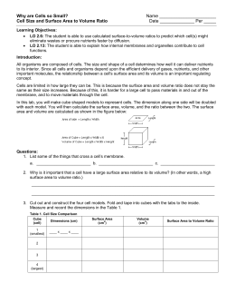


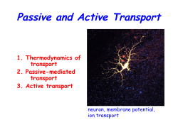


© Copyright 2026