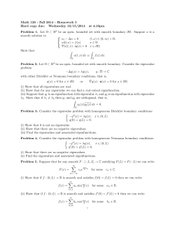
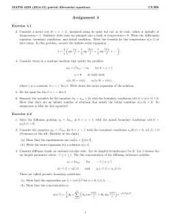
arXiv:1502.06800v1 [cs.LG] 24 Feb 2015
On the Equivalence between Quadrature Rules
and Random Features
Francis Bach
INRIA - Sierra project-team
D´epartement d’Informatique de l’Ecole Normale Sup´erieure
Paris, France
[email protected]
February 25, 2015
Abstract
We show that kernel-based quadrature rules for computing integrals are a special case
of random feature expansions for positive definite kernels for a particular decomposition
that always exists for such kernels. We provide a theoretical analysis of the number
of required samples for a given approximation error, leading to both upper and lower
bounds that are based solely on the eigenvalues of the associated integral operator and
match up to logarithmic terms. In particular, we show that the upper bound may
be obtained from independent and identically distributed samples from a known nonuniform distribution, while the lower bound if valid for any set of points. Applying our
results to kernel-based quadrature, while our results are fairly general, we recover known
upper and lower bounds for the special cases of Sobolev spaces. Moreover, our results
extend to the more general problem of full function approximations (beyond simply
computing an integral), with results in L2 - and L∞ -norm that match known results
for special cases. Applying our results to random features, we show an improvement
of the number of random features needed to preserve the generalization guarantees for
learning with Lipshitz-continuous losses.
1
Introduction
The numerical computation of high-dimensional integrals is one of the core computational
tasks in many areas of machine learning, signal processing and more generally applied mathematics, in particular in the context of Bayesian inference (Gelman, 2004), or the study of
complex systems (Robert and Casella, 2005). In this paper, we focus on quadrature rules,
that aim at approximating the integral of a certain function from only the (potentially
noisy) knowledge of the function values at as few as possible well-chosen points. The key
situations that remain active areas of research are problems where the measurable space
where the function is defined on, is either high-dimensional or structured (e.g., presence of
discrete structures, or graphs). For these problems, techniques based on positive definite
kernels have emerged as having the potential to efficiently deal with these situations, and to
1
improve over plain Monte-Carlo integration (O’Hagan, 1991; Rasmussen and Ghahramani,
2003; Husz´
ar and Duvenaud, 2012; Oates and Girolami, 2015). In particular, the quadrature problem may be cast as the one of approximating a fixed element, the mean element (Smola et al., 2007), of a Hilbert space as a linear combination of well chosen elements,
the goal being to minimize the number of these factors as it corresponds to the required
number of function evaluations.
A seemingly unrelated problem on positive definite kernels have recently emerged, namely
the representation of the corresponding infinite-dimensional feature space from random sets
of features. If a certain positive definite kernel between two points may be represented
as the expectation of the product of two random one-dimensional (typically non-linear)
features computed on these two points, the full kernel (and hence its feature space) may
be approximated by sufficiently many random samples, replacing the expectation by a
sample average (Neal, 1995; Rahimi and Recht, 2007; Huang et al., 2006). When using
these random features, the complexity of a regular kernel method such as the support
vector machine or ridge regression goes from quadratic in the number of observations to
linear in the number of observations, with a constant proportional to the number of random
features, which thus drives the complexity of these methods.
In this paper, we make the following contributions:
– We show in Section 3.2 that these two problems are equivalent; more precisely, kernelbased quadrature rules are a special case of random features for a particular decomposition that always exists for all positive definite kernels on a measurable space.
– We provide in Section 4 a theoretical analysis of the number of required samples for
a given approximation error, leading to both upper and lower bounds that are based
solely on the eigenvalues of the associated integral operator and match up to logarithmic
terms. In particular, we show that the upper bound may be obtained as independent
and identically distributed samples from a known non-uniform distribution, while the
lower bound if valid for any set of points.
– Applying our results to kernel quadrature, while our results is fairly general, we recover
known upper and lower bounds for the special cases of Sobolev spaces. Moreover, our
results extend to the more general problem of full function approximations (beyond
simply computing an integral), with results in L2 - and L∞ -norm that match known
results for special cases.
– Applying our results to random feature expansions, we show an improvement of the number of random features needed for preserving the generalization guarantees for learning
with Lipshitz-continuous losses.
2
Random Feature Expansions of Positive Definite Kernels
Throughout this paper, we consider a topological space X equipped with a Borel probability
measure dρ, which we assume to have full support. This naturally defines the space of
2
square-integrable functions1 . We consider a continuous positive definite kernel k : X × X →
R, that is a symmetric function such that for all finite families of points in X , the matrix of
pairwise kernel evaluations is positive semi-definite. This thus defines a reproducing kernel
Hilbert space (RKHS) F of functions from X to R, which we also assume separable. This
RKHS has two important properties (see, e.g., Berlinet and Thomas-Agnan, 2004): (a) for
any x ∈ X , the function k(·, x) : y 7→ k(y, x) is an element of F, and (b) we have the
reproducing property, that is, for all f ∈ F and x ∈ X , f (x) = hf, k(·, x)iF . We always
assume that F is infinite-dimensional.
Moreover, we assume that the function x 7→ k(x, x) is integrable with respect to dρ (which
is weaker than supx∈X k(x, x) < ∞). This implies that F is a subset of L2 (dρ); that is,
functions in the RKHS F are all square-integrable.
Z
f (x)k(x, y)dρ(y).
Integral operator. Let Σ : L2 (dρ) → L2 (dρ) be defined as (Σf )(x) =
X
R
Since X k(x, x)dρ(x) is finite, Σ is self-adjoint, positive semi-definite and trace-class. Moreover, Σ1/2 is a surjection from L2 (dρ) to F; more precisely, for any f ∈ F, there exists an
unique g ∈ (Ker Σ)⊥ ⊂ L2 (dρ) such that f = Σ1/2 g and kf kH = kgkL2 (dρ) (Smale and Cucker,
2001). This justifies the notation Σ−1/2 f for f ∈ F.
onig, 1986), there exMercer decomposition. From extensions of Mercer’s theorem (K¨
ists an orthonormal sequence (em )m>0 of L2 (dρ) and a summable non-increasing sequence
of strictly positive eigenvalues (µm )m>0 such that Σem = µm em . For simplicity we assume
that there are no zero eigenvalues, i.e., (em )m>0 is an orthonormal basis, which implies that
F is dense in L2 (dρ).
P
We have the decomposition k(x, y) = m>0 µm em (x)em (y). For each m > 0, the eigenfunc−1/2
1/2
tion em is an element of F and kem kF = µm ; moreover, (µm em )m>0 is an orthonormal
basis of F. This justifies
the view of F as the subspace of functions f ∈ L2 (dρ) such that
P
2
kΣ−1/2 f k2L2 (dρ) = m>0 µ−1
m hf, em iL2 (dρ) is finite.
Potential confusion with covariance operator. Note that the operator Σ is an operator on L2 (dρ). It should not ne confused with the (non-centered) covariance
operator C,
R
which is an autoadjoint operator on the RKHS F, defined by hg, Cf iF = X f (x)g(x)dρ(x).
Given that Σ1/2 is an isometry from L2 (dρ) to F, the operator C may also be used to define
an operator on L2 (dρ), which happens to be exactly Σ. Thus, the two operators have the
same eigenvalues.
2.1
Kernels as expectations
On top of the generic assumptions made above, we assume that there is another measurable
set V equipped with a probability measure dµ. We consider a function ϕ : V × X → R which
1
For simplicity we identify functions and their equivalence classes for the equivalence relationship of being
equal except for a zero-measure (for dρ) subset of X .
3
is square-integrable (for the measure dµ ⊗ dρ), and assume that the kernel k may be written
as, for all x, y ∈ X :
k(x, y) =
Z
V
ϕ(v, x)ϕ(v, y)dµ(v) = hϕ(·, x), ϕ(·, y)iL2 (dµ) .
(1)
In other words, for each v ∈ V, we have a one-dimensional feature ϕ(v, ·) which is a function
from X to R, and the kernel between x and y is simply the expectation of the dot-product
for this one-dimensional feature for v following the probability distribution dµ.
Such additional structure allows to give an explicit characterization of the RKHS F in terms
of the features ϕ. Indeed, as shown by Bach (2014, Z
App. A), a function f ∈ L2 (dρ) is in F
if and only if it may be written as ∀x ∈ X , f (x) =
V
g(v)ϕ(v, x)dµ(v) = hg, ϕ(·, x)iL2 (dµ) ,
for a certain function g : V → R such that kgk2L2 (dµ) is finite, with a norm kf k2F equal to
the minimum (which is always attained) of kgk2L2 (dµ) , over all possible decompositions of f .
2.2
Examples
In this section, we provide examples of kernels and usual decompositions. We first start by
decompositions that always exist, then focus on specific kernels based on Fourier components.
i h
i
X µm h
tr Σ)1/2 em (x) · tr Σ)1/2 em (x) ,
tr Σ
m>0
we obtain an expectation with V = N. In Section 3.2, we provide another generic decomposition with V = X .
Mercer decompositions.
From k(x, y) =
Periodic kernels on [0, 1]. We consider X = [0, 1] and translation-invariant kernels
k(x, y) of the form k(x, y) = t(x − y), where t is a square-integrable 1-periodic function.
These kernels are positive definite ifP
and only if the Fourier series
t is non-negative,
that is,
Pof
∞
∞
k(x, y) may be written
as k(x, y) = m=0 µm cos 2πm(x−y) = m=0 µm cos 2πmx cos 2πmy+
sin 2πmx sin 2πmy , with µm > 0, which can be put trivially as an expectation with V = Z.
These are the usual Fourier features (Rahimi and Recht, 2007). Moreover, the random
Fourier features correspond to the Mercer decomposition above for the uniform distribution
on [0, 1].
s−1
2s
(2π)
B2s ({x−
Among these, the sequence µ0 = 1 and µm = m12s leads to k(x, y) = 1+ (−1)2(2s)!
y}) where {x − y} denotes the fractional part of x − y (Wahba, 1990), and we recover the
traditional Sobolev space with parameter s > 1 (Adams and Fournier, 2003). For µn = r n ,
1−r cos 2π(x−y)
we have k(x, y) = 1−2r
, with a geometric decay of eigenvalues.
cos 2π(x−y)+r 2
Translation invariant kernels on R. We consider X = R and translation-invariant
kernels k(x, y) of the form k(x, y) = t(x − y), where t is an integrable function from R to
4
R. It is known that these kernels are positive definite if and only if the
R Fourier transform
of t is always a non-negative real number. More precisely, if tˆ(ω) = R t(x)e−iωx dx ∈ R+ ,
R
R
1
iω(x−y) dω = 1
ˆ
ˆ
then k(x, y) = 2π
R t(ω)e
2π R t(ω) cos ωx cos ωy + sin ωx sin ωy dω, which is
another form of random Fourier features with V = R and distribution with density tˆ(ω) (this
can be seen by splitting R into a positive part for the cosines and a negative part for the
sines). For these kernels, the decay of eigenvalues has been well-studied by Widom (1963),
who relate the decay of eigenvalues to the tails of the distribution dρ and the decay of the
Fourier transform of t. For example, for the Gaussian kernel on sub-Gaussian distributions,
the decay of eigenvalues is geometric, and for kernels leading to Sobolev spaces, the decay
is of the form m−2s . See also examples by Birman and Solomyak (1977).
Extensions to [0, 1]d and Rd . In order to extend to d > 1, we may consider several
extensions as described by Oates and Girolami (2015). We may first use the tensor product
of the d individual Hilbert spaces, for which the kernel is simply the product of individual
kernels. If each of the kernel leads to eigenvalues that are decaying as m−2s , then the
resulting eigenvalues decay as (log m)d−1 m−2s (see Appendix A), and thus up to logarithmic
terms at the same speed as d = 1. For Sobolev spaces of order s for each dimension, this
corresponds to functions which have square-integrable partial derivatives with all individual
orders less than s. This is to be contrasted with the usual multi-dimensional Sobolev space
which is composed of functions which have square-integrable partial derivatives with orders
with sum less than s. This last kernel leads to eigenvalues decaying as m−2s/d , which is
much slower (see Appendix A). Note that in terms of computation, there are extensions to
avoid linear complexity in d (Le et al., 2013).
2.3
Approximation from randomly sampled features
Given the formulation of k as an expectation in Eq. (1), it is natural to consider sampling
n elements P
v1 , . . . , vn ∈ V from the distribution dµ and define the kernel approximation
ˆ y) = 1 n ϕ(vi , x)ϕ(vi , y), which defines a finite-dimensional RKHS Fˆ .
k(x,
i=1
n
From the strong law of large numbers—which can be applied because we have the finite
1/2
ˆ y)
, when n tends to infinity, k(x,
expectation E|ϕ(v, x)ϕ(v, y)| 6 E|ϕ(v, x)|2 E|ϕ(v, y)|2
tends to k(x, y) almost surely, and thus we get as tight as desired approximations of the
kernel k, for a given pair (x, y) ∈ X ×X . Rahimi and Recht (2007) show that for translationinvariant kernels on a Euclidean space, then the convergence is uniform over a compact
√
subset of X , with the traditional rate of convergence of 1/ n.
ˆ the
In this paper, we rather consider approximations of functions in F by functions in F,
ˆ
ˆ
RKHS associated with k. A key difficulty is that in general F is not even included in F,
and therefore, we cannot use the norm in F to characterize approximations. In this paper,
we choose the L2 -norm associated with the probability measure dρ on X to characterize the
approximation. Given f ∈ F with norm kf kF less than one, we look for a function fˆ ∈ Fˆ
of the smallest possible norm and so that kf − fˆkL2 (dρ) is as small as possible.
5
Computation of error. Given the definition of the Hilbert space F in terms
P of ϕ, given
g ∈ L2 (dµ) with kgkL2 (dµ) 6 1, we aim at finding α ∈ Rn such that fˆ = ni=1 αi ϕ(vi , ·)
with norm kfˆk2Fˆ 6 nkαk22 6 1 as small as possible and with a small approximation error:
n
Z
X
ˆ
g(v)ϕ(v, ·)dµ(v)
kf − f kL2 (dρ) = αi ϕ(vi , ·) −
V
i=1
.
(2)
L2 (dρ)
Note that with αi = n1 g(vi ) and vi sampled from dµ, then, E(kαk22 ) 6 n1 and E(kf −
fˆk2L2 (dρ) ) 6 n1 supv∈V kϕ(v, ·)k2L2 (dρ) ; our goal is to obtain an error rate with a better scaling
in n, by (a) choosing a better distribution than dµ for the points v1 , . . . , vn and (b) by
finding the best possible weights α ∈ Rn (that may depend on the function g but not on f ).
Goals. We thus aim at sampling n points v1 , . . . , vn ∈ V from a distribution with density q with respect toPdµ. Then the kernel approximation using importance weights is
1
ˆ y) = 1 n
equal to k(x,
i=1 q(vi ) ϕ(vi , x)ϕ(vi , y) (so that the law of large numbers leads to
n
P
an approximation converging to k), and we thus aim to minimize ni=1 q(vβ)i1/2 ϕ(vi , ·) −
i
R
2 (which represents the norm of the approximation in
g(v)ϕ(v,
·)dµ(v)
,
with
nkβk
2
V
L2 (dρ)
ˆ
F) as small as possible.
3
Quadrature in RKHSs
Given a square-integrable (with Rrespect to dρ) function g : X → R, we aim
P at approximating, for all h ∈ F, integrals X h(x)g(x)dρ(x) by linear combinations ni=1 αi h(xi ) of
evaluations h(x1 ), . . . , h(xn ) of the function h at well-chosen points x1 , . . . , xn ∈ X . Of
course, coefficients α ∈ Rn are allowed to depend on g (they will in linear fashion in the
next section), but not on h.
3.1
Approximation of the mean element
Using the properties of RKHSs, the error is
n
X
i=1
αi h(xi ) −
Z
X
X
Z
n
k(·, x)g(x)dρ(x) ,
αi k(·, xi ) −
h(x)g(x)dρ(x) = h,
i=1
X
F
and by Cauchy-Schwarz inequality its supremum over khkF 6 1 is equal to
X
Z
n
k(·, x)g(x)dρ(x)
αi k(·, xi ) −
.
i=1
X
(3)
F
The goal of quadrature rules formulated in a RKHS is thus to find points x1 , . . . , xn ∈ X
and weights α ∈ Rn so that the quantity in Eq. (3) is as small as possible (Smola et al.,
6
2007). For g = 1, the function
distribution dρ.
R
X
k(·, x)dρ(x) is referred to as the mean element of the
The standard Monte-Carlo solution is to consider x1 , . . . , xn sampled i.i.d. from dρ and the
√
weights αi = g(xi )/n, which leads to a decrease of the error in 1/ n, with Ekαk22 6 n1 and
an expected squared error which is less than n1 supx∈X k(x, x) (Smola et al., 2007). Note
that when g = 1, Eq. (3) corresponds to particular metric between the distribution dρ and
its corresponding empirical distribution (Sriperumbudur et al., 2010).
In this paper, we explore sampling points xi from a probability distribution on X with
density q with respect to dρ. Note that when g is a constant function, it is sometimes
required that the coefficients α are positive and sum to a fixed constant (so that constant
functions are well integrated). We will not pursue this here as our theoretical results do not
accommodate such constraints.
Tolerance to noisy function values. In practice, independent (but not necessarily
identically distributed) noise may be present with variance σ 2 (xi ). Then,
the worst (with
P
n
respect to khkF 6 1) expected (with respect to the noise) squared error is
i=1 αi k(·, xi )−
2
R
Pn
2
2
i=1 αi σ (xi ), and thus in order to be robust to noise, having a
X k(·, x)g(x)dρ(x) F +
small weighted ℓ2 -norm for the coefficients α ∈ Rn is important.
3.2
Reformulation as random features
For any x ∈ X , we denote by ψ(·, x) the unique element of (KerP
Σ)⊥ ⊂ L2 (dρ) such that
1/2
Σ ψ(·, x) = k(·, x). Given the Mercer decomposition k(x, y) = m>0 µm em (x)em (y), we
P
1/2
have the expansion ψ(x, y) = m>0 µm em (x)em (y) (with convergence in the L2 -norm for
the measure dρ ⊗ dρ), and thus we may consider ψ as a symmetric function. Note that ψ
many not be easy to compute in many practical cases (except for periodic kernels on [0, 1]).
We thus have for (x, y) ∈ X × X :
k(x, y) = hk(·, x), k(·, y)iF = hψ(·, x), ψ(·, y)iL2 (dρ) =
Z
ψ(v, x)ψ(v, y)dρ(v).
X
That is, k may always be written as an expectation. Moreover, we have
X
Z
n
k(·,
x)g(x)dρ(x)
α
k(·,
x
)
−
i
i
i=1
X
F
X
Z
n
1/2
1/2
Σ ψ(x, ·)g(x)dρ(x)
= αi Σ ψ(xi , ·) −
X
F
i=1
Z
n
X
= ψ(x, ·)g(x)dρ(x)
αi ψ(xi , ·) −
,
i=1
X
L2 (dρ)
which is exactly an instance of the approximation result in Eq. (2) with V = X and ϕ = ψ.
Thus, the quadrature problem is a subcase of the random feature problem for a specific
expansion. Note that this random decomposition is always possible (although not in closed
form in general).
7
Goals. In order to be able to make the parallel with random feature approximation, we
consider importance-weighted
βi = αi q(xi )R1/2 , and we thus aim
Pncoefficients
at minimizing
−1/2
the approximation error
k(·, xi ) − X k(·, x)g(x)dρ(x) F . We consider
i=1 βi q(xi )
2
potential independent noise with variance σ (xi ) 6 τ 2 q(xi ) for all xi , so that the tolerance
to noise is characterized by the ℓ2 -norm kβk2 .
3.3
Related work on quadrature
Many methods have been designed for the computation of integrals of a function given
evaluations at certain well-chosen points, in most cases when g is constant equal to one.
We review some of these below.
Uni-dimensional integrals. When the underlying set X is a compact interval of the
real line, several methods exists, such as the trapezoidal or Simpson’s rules, which are
based on interpolation between the sample points, and for which the error decays as
O(1/n2 ) and O(1/n4 ) for functions with uniformly bounded second or fourth derivatives
(Cruz-Uribe and Neugebauer, 2002).
Gaussian quadrature is another class of methods for one-dimensional integrals: it is based
on a basis of orthogonal polynomials for L2 (dρ) where dρ is a probability measure supported
in an interval, and their zeros (Hildebrand, 1987, Chap. 8). This leads to quadrature rules
which are exact for polynomials of degree 2n−1 but error bounds for non-polynomials rely on
high-order derivatives, although the empirical performance on functions of a Sobolev space
is as good as optimal quadrature schemes (see Appendix B); depending on the orthogonal
polynomials, we get various quadrature rules, such as Gauss-Legendre quadrature for the
Lebesgue measure on [0, 1].
Quasi Monte-carlo methods employ a sequence of points with low discrepancy with uniform weights (Morokoff and Caflisch, 1994), leading to approximation errors of O(1/n) for
univariate functions with bounded variation, but typically with no adaptation to smoother
functions.
Higher-dimensional integrals. All of the methods above may be generalized for products of intervals [0, 1]d , typically with d small. For larger problems, Bayes-Hermite quadrature (O’Hagan, 1991) is essentially equivalent to the quadrature rules we study in this
paper.
Some of the quadrature rules are constrained to have positive weights with unit sum (so
that the positivity properties of integrals are preserved and constants are exactly inegrated).
The quadrature rules we present do not satisfy these constraints. If these constraints are
required, kernel herding (Chen et al., 2010; Bach et al., 2012) provides a novel way to select
a sequence of points based on the conditional gradient algorithm, but with currently no
√
convergence guarantees improving over O(1/ n) for infinite-dimensional spaces.
8
Theoretical results. The best possible error for a quadrature rule with n points has been
well-studied in several settings; see Novak (1988) for a comprehensive review. For example,
for X = [0, 1] and the space of Sobolev functions, which are RKHSs with eigenvalues of their
integral operator decreasing as m−2s , Novak (1988, Prop. 2 and 3, page 38) shows that the
best possible quadrature rule for the uniform distribution and g = 1 leads to an error rate of
n−s , as well as for any squared-integrable function g. The proof of these results (both upper
and lower bounds) relies on detailed properties of Sobolev spaces. In this paper, we recover
these results using only the decay of eigenvalues of the associated integral operator Σ, thus
allowing straightforward extensions to many situations, like Sobolev spaces on manifolds
such as hyperspheres (Hesse, 2006).
Moreover, Novak (1988, page 17) shows that adaptive quadrature rules where points are
selected sequentially with the knowledge of the function values at previous points cannot
improve the worst-case guarantees. Our results do not recover this lower bound result for
adaptivity.
From quadrature to function approximation and optimization. The problem of
quadrature, uniformly over all functions g ∈ L2 (dρ) that define the integral, is in fact
equivalent to the full approximation of a function h given values at n points, where the
approximation error is characterized in L2 -norm. Novak (1988) considers the approximation problem in L∞ -norm and shows that for Sobolev spaces, going from L2 - to L∞ -norms
√
incurs a loss of performance of n. We recover partially these results in Section 5 from
a more general perspective. When optimizing the points at which the function is evaluated (adaptively or not), the approximation problem is often referred to as experimental
design (Cochran and Cox, 1957; Chaloner and Verdinelli, 1995).
Finally, a third problem is of interest (and outside of the scope of this paper), namely the
problem of finding the minimum of a function given (potentially noisy) function evaluations.
For noiseless problems, Novak (1988, page 26) shows that the approximation and optimization problems have the same worst-case guarantees (with no influence of adaptivity); this
optimization problem has also been studied in the bandit setting (Srinivas et al., 2012) and
in the framework of “Bayesian optimization” (see, e.g. Bull, 2011).
4
Theoretical Analysis
In this section, we provide approximation bounds for the random feature problem outlined
in Section 2.3 (and thus the quadrature problem in Section 3). In Section 4.1, we provide
generic upper bounds, which depend on the eigenvalues of the integral operator Σ and
present matching lower bounds (up to logarithmic terms) in Section 4.2. We then consider
consequences of these results on quadrature (Section 4.3) and random feature expansions
(Section 4.4).
4.1
Upper bound
We have the following proposition (see proof in Appendix C.1):
9
1
Proposition 1 For λ > 0, we denote by dmax (q, λ) = supv∈V q(v)
hϕ(v, ·), (Σ+λI)−1 ϕ(v, ·)iL2 (dρ) .
Let v1 , . . . , vn be sampled i.i.d. from the distribution with positive density q with respect to
4dmax (q, λ)
, with probability greater than
dµ, then for any δ > 0, if n > 4 + 6dmax (q, λ) log
δ
1 − δ, we have
sup
kf kF 61
inf
4
kβk22 6 n
2
n
X
−1/2
f −
β
q(v
)
ϕ(v
,
·)
i
i
i
6 4λ.
L2 (dρ)
i=1
The proof technique relies on computing an explicit candidate β ∈ Rn obtained from minimizing a regularized least-squares formulation, leading to an approximation of f equal to
ˆ + λI)−1 Σf
ˆ , where Σ
ˆ is a properly defined empirical integral operator and λ > 0.
fˆ = (Σ
Then, Bernstein concentration inequalities for operators (Minsker, 2011) can be used in a
way similar to the work of Bach (2013); El Alaoui and Mahoney (2014) on column sampling.
Optimized distribution.
q(v) = R
We may now consider a specific distribution, namely
hϕ(v, ·), (Σ + λI)−1 ϕ(v, ·)iL2 (dρ)
hϕ(v, ·), (Σ + λI)−1 ϕ(v, ·)iL2 (dρ)
=
,
−1
tr Σ(Σ + λI)−1
V hϕ(v, ·), (Σ + λI) ϕ(v, ·)iL2 (dρ) dµ(v)
for which dmax (q, λ) = d(λ) = tr Σ(Σ + λI)−1 . We thus need to have n > 4 + 6d(λ) log 4d(λ)
δ
with d(λ) = tr Σ(Σ + λI)−1 is the degrees of freedom, a traditional quantity in the analysis
of least-squares regression (Hastie and Tibshirani, 1990), which is always smaller dmax (1, λ)
and can be upper-bounded explicitly for many examples as we now explain. The computation of dmax (1, λ) in the operator setting (for which we may use q = 1), a quantity often
referred to as the maximal leverage score (Mahoney, 2011), remains an open problem.
Eigenvalues and degrees of freedom. In order to relate
directly
eigenP more
P to theµm
µm
−1
values of Σ, we notice that d(λ) = tr Σ(Σ + λI)
=
>
µm >λ µm +λ >
P
P m>0 µmµ+λ
µm
1
m
µm > λ}). Moreover, d(λ) = µm >λ µm +λ + µm <λ µm +λ 6 max({m, µm >
2 max({m,
1 P
λ}) + λ µm <λ µm .
We now make the assumption that there exists γ > 0 such that
∀j > 1,
∞
X
µm 6 γjµj .
(4)
m=j
This assumption essentially states that the eigenvalues decay sufficiently homogeneously
and is satisfied by µm ∝ m−2α with γ = (2α − 1)−1 , µm ∝ r m with γ = (1 − r)−1 and
also for all examples in Section 2.2. It allows us to relate the degrees of freedom directly to
eigenvalue decays.
P
Indeed, this implies that λ1 µm <λ µm 6 γmax({m, µm > λ}) for all λ < µ0 and thus
10
1
2 max({m,
µm > λ}) 6 d 6 1 + γ max({m, µm > λ}).
From Prop. 1, we thus need to have, up to logarithmic terms, n > max({m, µm > λ})
random samples. For example, for polynomial decays of eigenvalues of the form µm =
O(m−2s ), we get errors proportional to n−s for n samples, while for geometric decays, we
get geometric errors.
4.2
Lower bound
We have the following lower bound (see proof in Appendix C.3):
Proposition 2 For δ ∈ (0, 1), if we have a family ψ1 , . . . , ψn ∈ L2 (dρ) such that
n
1X
kψi k2L2 (dρ) 6 4 tr Σ/δ,
n
and
i=1
then n >
sup
inf
4
kf kF 61 kβk22 6 n
max({m, µm > 144λ})
.
tr Σ
4 log 2 λδ
2
n
X
f −
βi ψi i=1
6 4λ,
L2 (dρ)
We can make the following observations:
– The proof technique not surprisingly borrows tools from minimax estimation over ellipsoids, namely the Varshamov-Gilbert’s lemma.
– We obtain matching upper and lower bounds up to logarithmic terms, using only the
decay of eigenvalues (µm ) of the integral operator Σ.
– In order to obtain such a bound, we need to constrain either kβk2 or the norms of the
vectors ψi , which corresponds to bounded features for the random feature interpretation
and tolerance to noise for the quadrature interpretation. We choose our scaling to match
the constraints we have in Prop. 1, in particular the bound shown in Eq. (7) in the proof
of Prop. 1 in Appendix C.1, for which the parameter δ ends up entering the lower bound
logarithmically.
4.3
Quadrature
We may specialize the results above to the quadrature case, namely give a formulation
where the features ϕ do not appear (or equivalently using ψ defined in Section 3.2). All
detailed computations are given in Appendix C.2.
If the points x1 , . . . , xn are sampled from the distribution with density q with respect to dρ,
then the quadrature rule becomes:
n
X
βi h(xi )
ˆ Σ
ˆ + λI)−1 Σ−1/2 h
= g, Σ1/2 Σ(
,
L2 (dρ)
1/2
q(xi )
i=1
11
−1 Σ−1/2 h
ˆ giL (dρ) with the approximation h
ˆ = Σ1/2 Σ(
ˆ Σ+λI)
ˆ
which can be put in the form hh,
2
of the function h ∈ F. Having a bound for all functions g such that kgkL2 (dρ) 6 1 is equivˆ L (dρ) . In Section 5, we consider extensions, where we
alent to having a bound on kh − hk
2
ˆ − h.
consider other norms than the L2 -norm for characterizing the approximation error h
Moreover, we consider cases, where h belongs to a strict subspace of F (with improved
results).
P
µm
2
Finally, the density q may be expressed as q(x) = m>0 µm
+λ em (x) . A weakness of our
result is that our optimized distribution q(x) = qλ (x) depends on λ and thus on the number of samples. In some cases with symmetries (i.e., uniform distribution on [0, 1] or the
hypersphere), qλ happens to be constant for all λ. Note also that typically qλ converges to
a certain distribution when λ tends to zero (see an example in Appendix B).
Recovering lower and upper bounds. For Sobolev spaces with parameters α in [0, 1]d
(for which we assume d < 2α), the decay of eigenvalues is of the form m−2α/d and thus the
error after n samples is n−α/d , which recovers the upper and lower bounds of Novak (1988,
pages 37 and 38).
P
be obtained by minimizing k ni=1 αi k(·, xi )−
RAlgorithms. The2quadrature weights α may
1 ⊤
⊤
2 α Kα− µ α, where K is the kernel matrix and
X g(x)k(·, x)dρ(x)kF , that is, minimizing
R
µ ∈ Rn the vector such that µi = X g(x)k(xi , x)dρ(x). Given these, which can be computed
in closed form for several triplet (k, g, dρ) (see, e.g., Smola et al., 2007; Oates and Girolami,
2015), we need to invert a linear system. Note that when adding points sequentially (in
particular for kernels for which the distribution qλ is independent of λ, such as Sobolev
spaces on [0, 1]), one may update the solution so that after n steps, the overall complexity
is O(n3 ).
4.4
Learning with random features
We consider supervised learning with m i.i.d. samples from a distribution on inputs/outputs
(x, y), and a uniformlyPG-Lipschitz-continuous loss function ℓ(y, ·). We consider the emˆ ) = 1 m ℓ(yi , f (xi )) and the expected risk L(f ) = Eℓ(y, f (x)), with x
pirical risk L(f
i=1
m
with marginal distribution dρ. We assume that Ek(x, x) = tr Σ = R2 . We have the usual
ˆ ) with respect to kf kF 6 F , based on
generalization bound for the minimizer fˆ of L(f
Rademacher complexity (see, e.g., Shalev-Shwartz and Ben-David, 2014):
E L(fˆ) 6
inf
kf kF 6F
L(f ) + 2E
h
i
ˆ )| 6
sup |L(f ) − L(f
kf kF 61
4F GR
.
L(f ) + √
m
kf kF 6F
inf
(5)
We now consider learning
n features, leading to a function parameterized by
Pn by sampling
n
−1/2
β ∈ R , that is gˆβ = i=1 βi q(vi )
ϕ(vi , ·) ∈ L2 (dρ). We assume that n is large enough
to have an expected squared error 8λ as in the end of the proof of Prop. 1 (Appendix C.1),
2
(if we consider the optimized distribution q). We consider
that is, n > 4 + 6d(λ) log R d(λ)
λ
√
ˆ
ˆ
a minimizer β of L(ˆ
gβ ) over kβk2 6 2F/ n. We obtain the following upper-bound on
12
E L(ˆ
gβˆ ) (for simplicity in expectation with respect to the data and the random features)
for the learned function gˆβˆ based on random features:
ˆ
E L(ˆ
gβˆ ) 6 inf L(f ) + E sup
inf √ |L(f ) − L(gβ )| + 2E sup √ |L(ˆ
gβ ) − L(ˆ
gβ )|.
kf kF 6F kβk2 62F/ n
kβkF 62F/ n
kf kF 6F
√
Because of the G-Lipschitz-continuity of the loss, the second term is less than GF 8λ. Following standard results for Rademacher complexities of ℓ2 -balls (Bartlett and Mendelson,
Pm Pn ϕ(vi ,xj )2 1/2
4F√G
4F√G
E
(nm tr Σ)1/2 =
6m
2003, Lemma 22), the third term is less than m
i=1
j=1 q(vi )
n
n
4F
√GR .
m
Overall, we obtain
E L(ˆ
gβˆ ) 6
√
4F GR
inf L(f ) + 3GF λ + √
.
m
kf kF 6F
The bound thus requires that we have λ = R2 /m and thus n > 4+6d(R2 /m) log md(R2 /m)
in order to lose only a constant factor compared to Eq. (5).
In the worst case, we have d(λ) 6 λ−1 tr Σ = R2 /λ, and thus n > 4 + 6m log m, and we
lose a logarithmic factor compared to Rahimi and Recht (2009). However, when we have
eigenvalue decays as R2 i−2s , we get (up to constants) d(λ) 6 (R2 /λ)1/(2s) , and thus n >
m1/(2s) log m, which is a significant improvement (regardless of the value of F ). Moreover,
if the decay is geometric as r i , then we get d(λ) 6 log(R2 /λ), and thus n > (log m)2 , which
is even more significant.
5
Quadrature-related Extensions
ˆ = Σ1/2 Σ(
ˆ Σ
ˆ + λI)−1 Σ−1/2 h of a function
In Section 4.3, we have built an approximation h
h ∈ F, which is based on n function evaluations h(x1 ), . . . , h(xn ). We have presented a
ˆ − hkL (dρ) for functions h with less than unit F-norm
convergence rate for the L2 -norm kh
2
khkF 6 1.
Robustness to noise. We have seen that if the noise in the function evaluations h(xi ) has
2
2
ˆ 2
a variance less than q(xi )τ 2 , then the error kh − hk
L2 (dρ) has an additional term τ kβk2 6
4τ 2
n .
Hence, the amount of noise has to be less than nµn in order to incur no loss in
performance (a bound which decreases with n).
Robustness to functions not in the RKHS. If the function h happens to be smoother
than elements of the RKHS F, that is, if kΣ−s hkL2 (dρ) 6 1, where s > 1/2, then we have
the error, w.h.p.,
ˆ − hkL (dρ) = λΣ1/2 (Σ
ˆ + λI)−1 Σ−1/2+s Σ−s h
kh
2
L2 (dρ)
1/2
−1/2
ˆ + λI)−1/2 Σ−1/2+s kΣ−s hkL (dρ)
ˆ + λI)
(Σ
6 λΣ (Σ
2
op
op
s−1 ˆ
1/2−s −1/2+s s
6 λ·2·λ
(Σ + λI)
Σ
6 4λ .
op
13
P
2s
The norm h 7→ kΣ−s hkL2 (dρ) is an RKHS norm with kernel
m>0 µm em (x)em (y), with
2s
corresponding eigenvalues equal to (µm ) . From Prop. 1 and 2, the optimal number
of quadrature points to reach a squared error less than ε is proportional to the number
max({m, µ2s
m > ε}), while using the quadrature points from s = 1/2, leads to a number
max({m, µm > ε1/(2s) }), which is equal. Thus if the RKHS used to compute the quadrature
weights is a bit too large (but not too large, see experiments in Appendix B), then we still
get the optimal rate. Note that this robustness is only shown for the regularized estimation
of the quadrature coefficients (in our simulations, the non-regularized ones also exhibit the
same behavior).
ˆ − h with different norms
Other norms. We may consider characterizing the difference h
−r
ˆ
than k · kL2 (dρ) , in particular norms kΣ (h − h)kL2 (dρ) , with r ∈ [0, 1/2]. We have:
ˆ − h)kL (dρ) = λΣ1/2−r (Σ
ˆ + λI)−1 Σ−1/2 h
kΣ−r (h
2
L2 (dρ)
1/2−r 1/2−r ˆ
r−1/2 6 λ
Σ
(Σ + λI)
kΣ−1/2 hkL2 (dρ) 6 2λ1/2−r .
op
When r = 1/2, we get a result in the RKHS norm, but with no decay to zero; the RKHS
norm k · kF would allow a control in L∞ -norm, but as noticed by Steinwart et al. (2009);
Mendelson and Neeman (2010), such a control may be obtained in practice with r much
smaller. For example, when the eigenfunctions em are uniformly bounded in L∞ -norm by a
constant C (as is the case for periodic kernels in [0, 1] with the uniform distribution), then,
for any x ∈ X , we have for t > 1,
2
f (x) 6
∞
X
t
(m + 1)
m=0
hf, em i2L2 (dρ)
∞
X
2
−t
em (x) (m + 1)
6
∞
X
(m + 1)t hf, em i2L2 (dρ)
m=0
m=0
C2
.
t−1
If for simplicity,Pwe assume that µm = (m + 1)−2s (like for Sobolev spaces), we have
t
2
−2s ) (as suggested
kΣ−r f k2L2 (dρ) = ∞
m=1 (m + 1) hf, em iL2 (dρ) with r = t/4s. If λ 6 O(n
1
1
λ1−2r = O t−1
n−2s(1−t/2s) =
by Prop. 1), then we obtain a squared error equal to t−1
n
nt −2s
, and thus a degradation compared to the
O t−1
n
. With t = 1 + log1 n , we get O nnlog
−2s
1/2
non-squared L2 -loss of n
(plus additional logarithmic terms), which corresponds to the
(non-improvable) result of Novak (1988, page 36).
6
Conclusion
In this paper, we have shown that kernel-based quadrature rules are a special case of random
feature expansions for positive definite kernels and derived upper and lower bounds on
approximations, that match up to logarithmic terms. For quadrature, this leads to widely
applicable results while for random features this allows a significantly improved guarantee
within a supervised learning framework.
The present work could be extended in a variety of ways, for example towards bandit optimization rather than quadrature (Srinivas et al., 2012), the use of quasi-random sampling
14
within our framework in the spirit of Yang et al. (2014); Oates and Girolami (2015), a similar analysis for kernel herding (Chen et al., 2010; Bach et al., 2012), an extension to fast
rates for non-parametric least-squares regression (Hsu et al., 2014) but with an improved
computational complexity, and a study of the consequences of our improved approximation
result for online learning and stochastic approximation, in the spirit of Dai et al. (2014);
Dieuleveut and Bach (2014).
Acknowledgements
This work was partially supported by the MSR-Inria Joint Centre and a grant by the
European Research Council (SIERRA project 239993). The author would like to thank the
STVI for the opportunity of writing a single-handed paper.
References
R. A. Adams and J. F. Fournier. Sobolev Spaces, volume 140. Academic Press, 2003.
F. Bach. Sharp analysis of low-rank kernel matrix approximations. In Proceedings of the
International Conference on Learning Theory (COLT), 2013.
F. Bach. Breaking the curse of dimensionality with convex neural networks. Technical
Report 01098505, HAL, 2014.
F. Bach, S. Lacoste-Julien, and G. Obozinski. On the equivalence between herding and conditional gradient algorithms. In Proceedings of the International Conference on Machine
Learning (ICML), 2012.
P. L. Bartlett and S. Mendelson. Rademacher and Gaussian complexities: Risk bounds and
structural results. Journal of Machine Learning Research, 3:463–482, 2003.
A. Berlinet and C. Thomas-Agnan. Reproducing Kernel Hilbert Spaces in Probability and
Statistics, volume 3. Springer, 2004.
R. Bhatia. Positive definite matrices. Princeton University Press, 2009.
M. Sh. Birman and M. Z. Solomyak. Estimates of singular numbers of integral operators.
Russian Mathematical Surveys, 32(1):15–89, 1977.
A. D. Bull. Convergence rates of efficient global optimization algorithms. Journal of Machine
Learning Research, 12:2879–2904, 2011.
K. Chaloner and I. Verdinelli. Bayesian experimental design: A review. Statistical Science,
10(3):273–304, 1995.
Y. Chen, M. Welling, and A. Smola. Super-samples from kernel herding. In Proceedings of
the Conference on Uncertainty in Artificial Intelligence (UAI), 2010.
W. G. Cochran and G. M. Cox. Experimental designs. John Wiley & Sons, 1957.
15
D. Cruz-Uribe and C. J. Neugebauer. Sharp error bounds for the trapezoidal rule and
Simpson’s rule. Journal of Inequalities in Pure and Applied Mathematics, 3(4), 2002.
B. Dai, B. Xie, N. He, Y. Liang, A. Raj, M.-F. Balcan, and L. Song. Scalable kernel methods
via doubly stochastic gradients. In Advances in Neural Information Processing Systems
(NIPS), 2014.
A. Dieuleveut and F. Bach. Non-parametric stochastic approximation with large step sizes.
Technical Report 1408.0361, ArXiv, 2014.
A. El Alaoui and M. W. Mahoney. Fast randomized kernel methods with statistical guarantees. Technical Report 1411.0306, arXiv, 2014.
A. Gelman. Bayesian Data Analysis. CRC Press, 2004.
T. J. Hastie and R. J. Tibshirani. Generalized Additive Models. Chapman & Hall, 1990.
K. Hesse. A lower bound for the worst-case cubature error on spheres of arbitrary dimension.
Numerische Mathematik, 103(3):413–433, 2006.
F. B. Hildebrand. Introduction to Numerical Analysis. Courier Dover Publications, 1987.
D. Hsu, S. M. Kakade, and T. Zhang. Tail inequalities for sums of random matrices that
depend on the intrinsic dimension. Electronic Communications in Probability, 17(14):
1–13, 2012.
D. Hsu, S. M. Kakade, and T. Zhang. Random design analysis of ridge regression. Foundations of Computational Mathematics, 14(3):569–600, 2014.
G.-B. Huang, Q.-Y. Zhu, and C.-K. Siew. Extreme learning machine: theory and applications. Neurocomputing, 70(1):489–501, 2006.
F. Husz´
ar and D. Duvenaud. Optimally-weighted herding is Bayesian quadrature. In
Proceedings of the Conference on Uncertainty in Artificial Intelligence (UAI), 2012.
H. K¨
onig. Eigenvalues of compact operators with applications to integral operators. Linear
Algebra and its Applications, 84:111–122, 1986.
Q. Le, T. Sarl´
os, and A. Smola. Fastfood: approximating kernel expansions in log-linear
time. In Proceedings of the International Conference on Machine Learning (ICML), 2013.
M. W. Mahoney. Randomized algorithms for matrices and data. Foundations and Trends
in Machine Learning, 3(2):123–224, 2011.
P. Massart. Concentration Inequalities and Model Selection: Ecole d’´et´e de Probabilit´es de
Saint-Flour 23. Springer, 2003.
S. Mendelson and J. Neeman. Regularization in kernel learning. The Annals of Statistics,
38(1):526–565, 2010.
S. Minsker. On some extensions of Bernstein’s inequality for self-adjoint operators. Technical
Report 1112.5448, arXiv, 2011.
16
W. J. Morokoff and R. E. Caflisch. Quasi-random sequences and their discrepancies. SIAM
Journal on Scientific Computing, 15(6):1251–1279, 1994.
R. M. Neal. Bayesian Learning for Neural Networks. PhD thesis, University of Toronto,
1995.
E. Novak. Deterministic and Stochastic Error Bounds in Numerical Analysis. SpringerVerlag, 1988.
C. J. Oates and M. Girolami. Variance reduction for quasi-Monte-Carlo. Technical Report
1501.03379, arXiv, 2015.
A. O’Hagan. Bayes-Hermite quadrature. Journal of statistical planning and inference, 29
(3):245–260, 1991.
A. Rahimi and B. Recht. Random features for large-scale kernel machines. In Advances in
Neural Information Processing Systems (NIPS), 2007.
A. Rahimi and B. Recht. Weighted sums of random kitchen sinks: Replacing minimization
with randomization in learning. In Advances in Neural Information Processing Systems
(NIPS), 2009.
C. E. Rasmussen and Z. Ghahramani. Bayesian Monte Carlo. In Advances in Neural
Information Processing Systems (NIPS), 2003.
C. P. Robert and G. Casella. Monte Carlo Statistical Methods. Springer New York, 2005.
S. Shalev-Shwartz and S. Ben-David. Understanding Machine Learning: From Theory to
Algorithms. Cambridge University Press, 2014.
S. Smale and F. Cucker. On the mathematical foundations of learning. Bulletin of the
American Mathematical Society, 39(1):1–49, 2001.
A. Smola, A. Gretton, L. Song, and B. Sch¨
olkopf. A Hilbert space embedding for distributions. In Algorithmic Learning Theory, pages 13–31. Springer, 2007.
N. Srinivas, A. Krause, S. M. Kakade, and M. Seeger. Information-theoretic regret bounds
for gaussian process optimization in the bandit setting. IEEE Transactions on Information Theory, 58(5):3250–3265, 2012.
B. K. Sriperumbudur, A. Gretton, K. Fukumizu, B. Sch¨
olkopf, and G. R. G. Lanckriet.
Hilbert space embeddings and metrics on probability measures. Journal of Machine
Learning Research, 11:1517–1561, 2010.
I. Steinwart, D. R. Hush, and C. Scovel. Optimal rates for regularized least squares regression. In Proceedings of the International Conference on Learning Theory (COLT),
2009.
G. Wahba. Spline Models for observational data. SIAM, 1990.
17
H. Widom. Asymptotic behavior of the eigenvalues of certain integral equations I. Transactions of the American Mathematical Society, 109:278–295, 1963.
J. Yang, V. Sindhwani, H. Avron, and M. Mahoney. Quasi-Monte Carlo feature maps
for shift-invariant kernels. In Proceedings of the International Conference on Machine
Learning (ICML), 2014.
L. Zwald, G. Blanchard, P. Massart, and R. Vert. Kernel projection machine: a new tool
for pattern recognition. In Advances in Neural Information Processing Systems (NIPS),
2004.
A
Eigenvalues for tensor products
Given a kernel k on the set X , with eigenvalues (µm )m>0 with respect to the measure dρ,
there are mainly three ways to define a kernel K on X = (x1 , . . . , xd ) ∈ X d with the product
probability distribution (dρ)⊗d :
P
– Sum: K(X, Y ) = dj=1 k(xj , yj ). Its eigenvalues are µm , m > 0, each with multiplicity
d. Thus, if µm ∝ m−2s , we have a number of eigenvalues of K greater than λ equivalent
to dλ−1/(2s) .
Q
– Product: K(X, Y ) = dj=1 k(xj , yj ). Its eigenvalues are µm1 ×· · ·×µmd , m1 , . . . , md >
0. Thus, if µm ∝ m−2s , we have a number of eigenvalues of K greater than λ equivalent
to the number of multi-indices such that m1 × · · · × md less than λ−1/(2s) , which can
easily be upper bounded by λ−1/(2s) (log λ−1 )d−1 .
P
1/d
– Harmonic means of eigenvalues. If m>0 µm is finite, we may define
K(X, Y ) =
X
m1 ,...,md >0
with eigenvalues
Pd d
−1
j=1 µmj
6
Qd
d
j=1 µmj
d
Y
emj (xj )emj (yj ),
−1
j=1 µmj j=1
Pd
1/d
(and hence summable). For F a Sobolev
space in 1 dimension, we obtain the regular Sobolev space in d dimensions. That is, for
2s > d, if µm ∝ m−2s , we have a number of eigenvalues of K greater than λ equivalent
to the number of multi-indices such that kmk2s 6 (λ/d)−1/(2s) , which can easily be
upper bounded by a constant times λ−d/(2s) .
B
Simulations
In this section, we consider
simple illustrative quadrature experiments with X = [0, 1] and
P
1
kernels k(x, y) = 1 + ∞
m=1 m2s cos 2πm(x − y), with various values of s and distributions
dρ which are Beta random variable with the two parameters equal to a = b.
18
Uniform distribution. For b = 1, we have the uniform distribution on [0, 1] for which the
cosine/sine basis
R 1 is orthonormal, and the optimized distribution qλ is also uniform. Moreover, we have 0 k(x, y)dρ(x) = 1. We report results comparing different Sobolev spaces for
testing functions to integrate (parameterized by s) and learning quadrature weights (parameterized by t) in Figure 1, where we compute errors averaged over 1000 draws. We did
not use regularization to compute weights α. We can make the following observations:
– The exponents in the convergence rates for s = t (matching RKHSs) are close to 2s
as expected.
– When the functions to integrate are less smooth than the ones used for learning (that
is t > s), then the quadrature performance does not necessarily decay with the number
of samples.
– On the contrary, when s > t, then we have convergence and the rate is potentially
worse than the optimal one (attained for s = t), and equal when t > s/2.
In Figure 2, we compare several quadrature rules on [0, 1], namely Simpson’s rule with
uniformly spread points, Gauss-Legendre quadrature and the Sobol sequence with uniform
weights. For s = 1, all squared errors decay as n−2 with a worse constant for our kernelbased rule (which is the only one with such a general applicability), while for s = 2, the
Sobol sequence is not adaptive.
Non-uniform distribution. In order to compute
R 1 the weights and the error from points
x1 , . . . , xn , we need to compute for all y ∈ [0, 1], 0 k(x, y)p(x)dx. In order to compute the
optimal density q(x) from Eq. (8), we may take a set of y1 , . . . , ym uniformly spread in [0, 1],
for m large, and compute
hk(·, x), Σ−1 k(·, yi )iL2 (dρ) = k(x, yi )
Z 1
k(x, yj )k(x, yi )dρ(x),
hk(·, yi ), k(·, yj )iL2 (dρ) =
0
to estimate coordinates of the approximation of the operator Σ−1 on the large independent
set {k(·, y1 ), . . . , k(·, ym )}.
All of these are computed by Gauss-Chebyshef quadrature with 10000 points. In Figure 3,
we compare several distributions q(x). The distribution a = b = .25 happens to be the limit
of qλ as λ tends to zero. All distributions achieve the optimal rate O(n−2 ) except the one
with a = b = 2, illustrating the fact that wrong distributions may have an adverse impact.
C
C.1
Proofs
Proof of Prop. 1
R
Any f ∈ F with F-norm less than one, may be represented as f = V g(v)ϕ(v, ·)dµ(v),
for a certain g ∈ L2 (dµ) with L2 (dµ)-norm less than one. We do not solve the problem
19
Test functions : s = 1
Test functions : s = 2
0
t=1 : 2.0
t=2 : 2.2
t=3 : 3.2
t=4 : 5.1
2
log10(squared error)
log10(squared error)
4
0
−2
−1
−2
−3
−4
−5
−6
0
0.5
1
1.5
log10(n)
2
0
Test functions : s = 3
log10(squared error)
log10(squared error)
1
1.5
log10(n)
2
0
−2
−4
−6
−10
0
0.5
Test functions : s = 4
0
−8
t=1 : 3.8
t=2 : 3.8
t=3 : 3.8
t=4 : 4.9
t=1 : 4.2
t=2 : 5.6
t=3 : 5.6
t=4 : 5.6
0.5
1
1.5
log10(n)
−2
−4
−6
−8
−10
−12
2
0
t=1 : 4.2
t=2 : 7.0
t=3 : 7.2
t=4 : 7.1
0.5
1
1.5
log10(n)
2
Figure 1: Quadrature for functions in a Sobolev space with parameter s (four possible
values) for the uniform distribution on [0, 1], with quadrature rules obtained from different
Sobolev spaces with parameters t (same four possible values). We compute affine fits in
log-log-space to estimate convergence rates of the form C/nu and report the value of u.
Best seen in color.
20
Test functions : s = 1
Test functions : s = 2
0
log10(squared error)
log10(squared error)
0
−1
−2
−3
−4
0
Sobol : 1.8
Simpson : 2.0
Kernel : 2.0
Legendre : 2.0
0.5
−2
−4
−6
−8
1
1.5
log10(n)
2
0
Sobol : 2.1
Simpson : 4.0
Kernel : 3.8
Legendre : 4.0
0.5
1
1.5
log10(n)
2
Figure 2: Quadrature for functions in a Sobolev space with parameters s = 1 (left) and
s = 2 (right), for the uniform distribution on [0, 1], with various quadrature rules. We
compute affine fits in log-log-space to estimate convergence rates of the form C/nu and
report the value of u. Best seen in color.
Beta distribution : s = 1
0
log10(squared error)
−0.5
−1
−1.5
−2
−2.5
−3
−3.5
0
a=b=.25 : 2.0
a=b= .5 : 2.0
a=b=.75 : 2.0
a=b= 1 : 1.9
a=b= 2 : 1.0
0.5
1
1.5
log10(n)
2
Figure 3: Quadrature for functions in a Sobolev space with parameter s = 1 for the Beta
distribution on [0, 1] with parameters a = b = 1/2, with quadrature rules obtained from
sampling from different Beta distributions with equal parameters a = b. We compute affine
fits in log-log-space to estimate convergence rates of the form C/nu and report the value of
u. Best seen in color.
21
in β exactly, but use a properly chosen Lagrange multiplier λ and consider the following
minimization problem:
n
2
Z
X
−1/2
+ nλkβk22 .
ϕ(v, ·)g(v)dµ(v)
βi q(vi )
ϕ(vi , ·) −
X
i=1
L2 (dρ)
By introducing the notation Φ which is a matrix with infinitely many rows and i-th column
equal to q(vi )−1/2 ϕ(vi , ·) ∈ L2 (dρ), we need to minimize the familiar least-squares problem:
f − Φβ 2
+ nλkβk22 ,
L2 (dρ)
with solution from the usual normal equations and the matrix inversion lemma:
β = (Φ⊤ Φ + nλI)−1 Φ⊤ h =
1 ⊤ 1
Φ ( ΦΦ⊤ + λI)−1 f.
n
n
(6)
ˆ : L2 (dρ) → L2 (dρ), defined as
We consider the operator Σ
n
X 1
ˆ = 1 ΦΦ⊤ = 1
ϕ(vi , ·) ⊗L2 (dρ) ϕ(vi , ·),
Σ
n
n
q(vi )
i=1
ˆ L (dρ) =
that is, for a, b ∈ L2 (dρ), ha, Σbi
2
n
X
ha, ϕ(vi , ·)iL2 (dρ) hb, ϕ(vi , ·)iL2 (dρ)
q(vi )
i=1
.
ˆ allows us to make more formal the heuristic computations above.
This operator Σ
ˆ + λI)−2 f
ˆ + λI)−1 f
The value of kf − Φβk2L2 (dρ) is equal to λ2 f, (Σ
6
λ
f,
(
Σ
.
L2 (dρ)
L2 (dρ)
ˆ + λI)−1 f , and
Finally, we have, with β = n1 Φ⊤ (Σ
ˆ + λI)−1 f, Σ(
ˆ Σ
ˆ + λI)−1 f
kβk22 = (Σ
L2 (dρ)
ˆ + λI)−1 f
6 f, (Σ
.
L2 (dρ)
ˆ = Σ. Moreover, we have, by Cauchy-Schwarz inequality:
By construction, we have E(Σ)
2
2 Z Z
Z
a(x)g(v)ϕ(v, x)dµ(v)dρ(x)
a(x)f (x)dρ(x) =
ha, (f ⊗L2 (dρ) f )aiL2 (dρ) =
6
Z
X
V
X
V
2
2Z Z
a(x)ϕ(v, x)dρ(x) dµ(v) 6 ha, ΣaiL2 (dρ) .
g(v)2 dµ(v)
V
X
Thus f ⊗L2 (dρ) f 4 Σ (with the classical partial order between self-adjoint operators), and
we may thus define hf, Σ−1 f iL2 (dρ) , which is less than one.
ˆ + λI)−1 f iL (dρ) , for hf, Σ−1 f iL (dρ) 6 1, to control both the
Overall we aim to study hf, (Σ
2
2
norm kβk22 and the approximation error. We have, following a similar argument than the
one of Bach (2013); El Alaoui and Mahoney (2014) for column sampling:
ˆ + λI)−1 f iL (dρ)
hf, (Σ
2
ˆ − Σ)−1 f iL (dρ)
= hf, (Σ + λI + Σ
2
−1/2
ˆ − Σ)(Σ + λI)−1/2 −1 (Σ + λI)−1/2 f iL (dρ) .
= h(Σ + λI)
f, I + (Σ + λI)−1/2 (Σ
2
22
ˆ − Σ)(Σ + λI)−1/2 < −tI, with t ∈ (0, 1), we have
Thus, if (Σ + λI)−1/2 (Σ
ˆ + λI)−1 f iL (dρ) 6 (1 − t)−1 hf, (Σ + λI)−1 f iL (dρ)
hh, (Σ
2
2
6 (1 − t)−1 hf, Σ−1 hiL2 (dρ) 6 (1 − t)−1 .
ˆ
Thus, the performance depends on having (Σ + λI)−1/2 (Σ − Σ)(Σ
+ λI)−1/2 4 tI. We
1
1
1
consider the self-adjoint operators Xi = n (Σ + λI)−1 Σ − n q(vi ) (Σ + λI)−1/2 ϕ(vi , ·) ⊗L2 (dρ)
(Σ + λI)−1/2 ϕ(vi , ·) , so that our goal is to provide an upperbound on the probability that
R hϕ(v,·),(Σ+λI)−1 ϕ(v,·)iL2 (dρ)
P
k ni=1 Xi kop > t. We denote by d = tr Σ(Σ+λI)−1 = V
q(v)dµ(v) 6
q(v)
dmax . We have EXi = 0, kXi kop 6
n
X
E(Xi2 )
4
i=1
dmax
n
and
hϕ(v, ·), (Σ + λI)−1 ϕ(v, ·)iL2 (dρ)
1
E
n
q(v)2
dmax
−1/2
−1/2
(Σ + λI)−1 Σ,
· (Σ + λI)
ϕ(v, ·) ⊗ (Σ + λI)
ϕ(v, ·) 4
n
dmax
dmax
with a maximal eigenvalue less than
and a trace less than
tr Σ(Σ + λI)−1 =
n
n
d dmax
.
n
Following Hsu et al. (2014), we use a matrix Bernstein inequality which is independent of
the underlying dimension (which is here infinite). We consider the bound of Minsker (2011,
Theorem 2.1), which improves on the earlier result of Hsu et al. (2012, Theorem 4), that is:
X
n
Xi P i=1
>t
op
6 2d 1 +
6d2max
n2 log2 (1 + t)
exp
−
nt2
.
2dmax (1 + 3t)
4dmax
We now consider t = 34 , δ ∈ (0, 1), and n > 4 + 6dmax log
> 10dmax . This implies
δ
that
6d2max
δ
δ
6
nt2
, and 1+ 2
6
6
6 1+
6 2.
exp −
2dmax (1 + 3t)
4dmax
4d
n log2 (1 + t)
100 log 2 (7/4)
Thus the probability is less than δ. We can make the following extra observations regarding
the proof:
– It may be possible to derive a similar result with a thresholding of eigenvalues in
the spirit of Zwald et al. (2004), but this would require Bernstein-type concentration
inequalities for the projections on principal subspaces.
– Note that A 4 B does not imply in A2 4 B 2 (Bhatia, 2009, page 9) and that in
ˆ + λI)−2 4 C(Σ + λI)−2 for any constant C (which would
general we do not have (Σ
allow an improvement in the error by replacing λ by λ2 , and violate the lower bound
of Prop. 2).
23
– We may also obtain a result in expectation, by using δ = 4λ/ tr Σ (which is assumed
to be less than 1), leading to a squared error with expectation less than 8λ as soon as
n > 4 + 6dmax (λ) log (tr Σ)dλmax (λ) . We use this result in Section 4.4.
R
ˆ = tr Σ =
– We have E tr Σ
X k(x, x)dρ(x), and thus, by Markov’s inequality, with
probability 1 − δ,
ˆ 6 1 tr Σ.
(7)
tr Σ
δ P
By taking δ/2 instead of δ in the control of k ni=1 Xi kop > t, we have a control over
ˆ and the approximation error. This will be useful for the lower bound of
kβk22 , tr Σ
Prop. 2.
C.2
Application to quadrature
In this section, we specialize the results from the section above to the quadrature subcase,
namely we give a formulation where the features ϕ do not appear (or equivalently using ψ
defined in Section 3.2).
We assume that points x1 , . . . , xn are sampled
from the distribution with
R
R density q with respect to dρ. We aim to write f ∈ F as f = X ψ(x, ·)g(x)dρ(x) = Σ−1/2 X k(x, ·)g(x)dρ(x) =
Σ1/2 g. Moreover, we have
X
n
n
1
1X 1
−1/2 1
ˆ
ψ(xi , ·) ⊗L2 (dµ) ψ(xi , ·) = Σ
k(xi , ·) ⊗L2 (dµ) k(xi , ·) Σ−1/2 .
Σ=
n
q(vi )
n
q(vi )
i=1
i=1
and we have
hf, Σ
1/2 ˆ
ΣΣ
1/2
giL2 (dρ) =
n
X
i=1
1
q(xi )
Z
X
Z
k(xi , y)g(y)dρ(y) .
k(xi , y)f (y)dρ(y)
X
ˆ + λI)−1 Σ1/2 giL (dρ) , and the quadraWe have from Eq. (6) βi = nq(x1 )1/2 hk(·, xi ), Σ−1/2 (Σ
2
i
ture rule becomes:
n
n
X
X
βi
βi h(xi )
=
hh, Σ−1 k(·, xi )iL2 (dρ)
1/2
1/2
q(x
)
q(x
)
i
i
i=1
i=1
n
−1/2
1 X −1 1 −1 1/2
ˆ
Σ
k(xi , ·) ⊗L2 (dµ) k(xi , ·) Σ
(Σ + λI) Σ g
= h,
n
q(xi )
L2 (dρ)
i=1
−1/2 ˆ ˆ
−1 1/2
1/2 ˆ ˆ
−1 −1/2
= h, Σ
Σ(Σ + λI) Σ g L2 (dρ) = g, Σ Σ(Σ + λI) Σ
h L2 (dρ) ,
−1 Σ−1/2 h.
ˆ giL (dρ) with the approximation h
ˆ = Σ1/2 Σ(
ˆ Σ+λI)
ˆ
which can be put in the form hh,
2
Finally, the density q may be expressed as
q(x) ∝ hk(·, x), Σ−1/2 (Σ + λI)−1 Σ−1/2 k(·, x)iL2 (dρ) =
X
i∈I
µi
ei (x)2 .
µi + λ
An alternative expression that can be used to compute q in practise is
q(x) ∝ hk(·, x), (I + λΣ−1 )−1 k(·, x)iL2 (dρ) .
24
(8)
C.3
Proof of Prop. 2
We first use the Varshamov-Gilbert’s lemma (see, e.g., Massart, 2003, Lemma 4.7). That
is, for an integer s, there exists a family (θj )j∈J of at most |J| > es/8 distinct elements of
{0, 1}s , such that for j 6= j ′ ∈ J, kθj − θj ′ k22 > 4s .
For
each θ ∈ {0, 1}s , we define an element of F with norm less than one, as f (θ) =
√
P
µ
s
√s
i=1 θi ei , where (ei , µi ), i = 1, . . . , s are the eigenvector/eigenvalue pairs associated
s
with the s largest eigenvalues of Σ. We indeed have
kf (θ)k2F =
s
µs X 2 −1
θi µi 6 1.
s
i=1
Moreover, for any j 6= j ′ ∈ J, we have kf (θj ) − f (θj ′ )k2L2 (dρ) = µss kθj − θj ′ k22 > µ4s .
q
√
Thus, if 4λ 6 µ4s /3, then there exists a family (βj )j∈J of elements of Rn , with squared
P
ℓ2 -norm less than n4 , and for which for any j 6= j ′ ∈ J, we have ni=1 (βj − βj ′ )i ψi L2 (dρ) >
q
µs
−1 tr Σ)kβ − β ′ k2 > (β − β ′ )⊤ Ψ⊤ Ψ(β − β ′ ) > µs , that is
j
j
j
j
j
j 2
4 /3. This implies n(4δ
36
q
δµs
s/8
kβj − βj ′ k2 >
= ∆. Thus, e
is less than the packing number of the sphere
√144n tr Σ
of radius r = 2/ n, which is itself less than (r/∆)n (2 + ∆/r)n (see, e.g., Massart, 2003,
Lemma 4.14). Since ∆/r 6 1/24, we have
1
36 tr Σ
s
6n
log
+ log(2 + 1/24) .
8
2
δµs
This implies n >
s
4 log
tr Σ
+21
δµs
. Given that we have to choose µs > 144λ for the result to hold,
this implies the desired result.
25