
PROJECTE DE TESIS
Nom/Logotip de la
Universitat on s’ha
llegit la tesi
Quantifying the effects of soil and climate on grape and
wine quality : applicaton in a viticultural zoning based
on very detailed soil surveys
Josep Miquel Ubalde Bauló
Dipòsit Legal: L.960-2013
http://hdl.handle.net/10803/123551
ADVERTIMENT. L'accés als continguts d'aquesta tesi doctoral i la seva utilització ha de respectar els drets
de la persona autora. Pot ser utilitzada per a consulta o estudi personal, així com en activitats o materials
d'investigació i docència en els termes establerts a l'art. 32 del Text Refós de la Llei de Propietat Intel·lectual
(RDL 1/1996). Per altres utilitzacions es requereix l'autorització prèvia i expressa de la persona autora. En
qualsevol cas, en la utilització dels seus continguts caldrà indicar de forma clara el nom i cognoms de la
persona autora i el títol de la tesi doctoral. No s'autoritza la seva reproducció o altres formes d'explotació
efectuades amb finalitats de lucre ni la seva comunicació pública des d'un lloc aliè al servei TDX. Tampoc
s'autoritza la presentació del seu contingut en una finestra o marc aliè a TDX (framing). Aquesta reserva de
drets afecta tant als continguts de la tesi com als seus resums i índexs.
ADVERTENCIA. El acceso a los contenidos de esta tesis doctoral y su utilización debe respetar los
derechos de la persona autora. Puede ser utilizada para consulta o estudio personal, así como en
actividades o materiales de investigación y docencia en los términos establecidos en el art. 32 del Texto
Refundido de la Ley de Propiedad Intelectual (RDL 1/1996). Para otros usos se requiere la autorización
previa y expresa de la persona autora. En cualquier caso, en la utilización de sus contenidos se deberá
indicar de forma clara el nombre y apellidos de la persona autora y el título de la tesis doctoral. No se
autoriza su reproducción u otras formas de explotación efectuadas con fines lucrativos ni su comunicación
pública desde un sitio ajeno al servicio TDR. Tampoco se autoriza la presentación de su contenido en una
ventana o marco ajeno a TDR (framing). Esta reserva de derechos afecta tanto al contenido de la tesis como
a sus resúmenes e índices.
WARNING. Access to the contents of this doctoral thesis and its use must respect the rights of the author. It
can be used for reference or private study, as well as research and learning activities or materials in the
terms established by the 32nd article of the Spanish Consolidated Copyright Act (RDL 1/1996). Express and
previous authorization of the author is required for any other uses. In any case, when using its content, full
name of the author and title of the thesis must be clearly indicated. Reproduction or other forms of for profit
use or public communication from outside TDX service is not allowed. Presentation of its content in a window
or frame external to TDX (framing) is not authorized either. These rights affect both the content of the thesis
and its abstracts and indexes.
QUANTIFYING THE EFFECTS OF SOIL AND CLIMATE
ON GRAPE AND WINE QUALITY:
Application in a Viticultural Zoning based on
very detailed Soil Surveys
Josep Miquel Ubalde Bauló
QUANTIFYING THE EFFECTS OF SOIL AND CLIMATE
ON GRAPE AND WINE QUALITY:
Application in a Viticultural Zoning based on
very detailed Soil Surveys
Thesis submitted in fulfilment of the requirements for the degree of Doctor
in Environment and Soil Science in the University of Lleida
Author:
Josep Miquel Ubalde Bauló
Directors:
Dra. Rosa Maria Poch i Claret
Dr. Xavier Sort Camañes
2010
Department of Viticulture, Miguel Torres Winery
Department of Environment and Soil Science, University of Lleida
Tu ne quaesieris (scire nefas) quem mihi, quem tibi
finem di dederint, Leuconoe, nec Babylonios
temptaris numeros. Vt melius, quidquid erit, pati!
seu pluris hiemes, seu tribuit Iuppiter ultimam,
quae nunc oppositis debilitat pumicibus mare
Tyrrhenum: sapias, uina liques et spatio breui
spem longam reseces. Dum loquimur, fugerit inuida
aetas: carpe diem, quam minimum credula postero.
Horace (65 - 8 BC)
ii
iii
AGRAÏMENTS (Acknowledgements)
A l’empresa Miguel Torres S.A., que ha finançat gran part d’aquest estudi, així com a
Xavier Sort, que ha dirigit la tesi, i a altres companys de l’empresa, que m’han aportat tots
els coneixements de viticultura i enologia que m’han fet falta.
A la Universitat de Lleida, pels diferents serveis dels que s’ha pogut disposar
(micromorfologia, hidrologia, SIG, biblioteca). A la Rosa Maria Poch, que també ha
dirigit la tesi i m’ha motivat i animat tots aquests anys per tirar-la endavant. Al Jaume
Boixadera, que ha tingut un paper fonamental en la meva formació de cartografia de sòls.
A tots els col·laboradors de la Universitat de Lleida que han participat activament en
aquest estudi.
Als editors de les revistes que han confiat amb els articles que formen part d’aquesta tesi i
als revisors anònims que han fet aportacions que han millorat els resultats finals.
A la meva família i amics, que han estat sempre al meu costat, donant-me suport tant en
els bons moments com en els no tant bons.
Josep Miquel Ubalde Bauló
Vilafranca del Penedès, 8 de març de 2010
i
CONTENTS
Abstract
ix
Resum (abstract in Catalan)
x
Resumen (abstract in Spanish)
xi
Account
xii
Chapter 1. General introduction: What is viticultural zoning?
1
Chapter 2. Application of a very detailed soil survey method in viticultural
9
zoning at plot level
Chapter 3. How soil forming processes determine a viticultural zoning based on
29
very detailed soil surveys
Chapter 4. Characterization of the soil moisture regime for viticultural zoning
49
purposes
Chapter 5. Influence of soil and climate on grape harvest quality at plot level
67
Chapter 6. Effects of soil and climate on grape ripening and wine quality of
81
Cabernet Sauvignon
Chapter 7. Global discussion
99
Chapter 8. Final conclusions
103
References
107
vii
viii
ABSTRACT
This study, carried out in vineyards of high quality wine production in Catalonia (Spain), aims
to determine the suitability of very detailed soil surveys, based on Soil Taxonomy, for
viticultural zoning purposes, and quantifies the effects of soil and climate on grape and wine
quality in some representative soil map units. After an introductory chapter, this objective is
developed in different chapters. Chapter 2 analyses the suitability of soil map units,
determined at a 1:5,000 scale according to Soil Taxonomy classification, to determine
important edaphic properties for vineyard growing. A k-means clustering analysis is proposed
in order to group soils according to their potential for vine growing, since most of the
variability of soil properties was not reflected exactly in the soil map unit classification.
Chapter 3 discusses the implications of soil forming processes on very detailed soil surveys.
The identified soil forming processes had significant effects on soil properties which are
important for vineyard growing. However, soil forming processes were not always reflected
in soil classification, especially in soils modified by man. Chapter 4 analyses the suitability of
Soil Taxonomy to characterize the soil moisture regime for viticultural zoning purposes. A
soil moisture regime classification based on cluster analysis was developed, since Soil
Taxonomy did not adequately reflect the variability of soil moisture dynamics during
vineyard growing. Chapter 5 focuses on the influence of soil and climate on vintage
variability. Climate and soil moisture explained 70% of vintage variability and soil properties
explained 28% of variability. Generally, climate was the most influential factor on must
composition, while soil factor mostly affected yield. Chapter 6 determines the effects of
climate and soil on grape ripening and wine quality of Cabernet Sauvignon. Climate and soil
had overall a significant effect on grape ripening. These effects of soil and climate can be
explained mainly by their influence on vine water availability status. Soil was determining in
wine phenolic composition, and related wine tasting characteristics. As a final conclusion,
very detailed soil surveys based on Soil Taxonomy are valuable sources of information for
viticultural zoning studies, although their implementation can be improved with statistical
analysis that considers the variability of soil properties related to grapevine growing.
Moreover, although climate explains most of the vintage variability, soil type is decisive in
determining the vineyard potential for wine quality.
ix
RESUM
L’objectiu d’aquest estudi, dut a terme en vinyes destinades a la producció de vi de qualitat a
Catalunya (Espanya), és determinar si un mapa de sòls molt detallat, basat en la Soil
Taxonomy, és apte per estudis de zonificació vitícola i quantificar els efectes del sòl i el clima
sobre la qualitat del raïm i del vi, en unitats cartogràfiques representatives. Després d’un
capítol introductori, aquest objectiu es desenvolupa en diferents capítols. El capítol 2 analitza
l’aptitud d’unitats cartogràfiques de sòls, classificades segons la Soil Taxonomy, per reflectir
la variabilitat de propietats edàfiques importants per al cultiu de la vinya. Degut a què aquesta
variabilitat no es reflectia exactament en la classificació de les unitats cartogràfiques, es va
proposar una anàlisi clúster per agrupar els sòls segons el seu potencial vitícola. En el capítol
3 es discuteixen les implicacions dels processos formadors del sòl en la cartografia de sòls
molt detallada. Els processos formadors identificats tenien efectes significatius sobre
propietats edàfiques importants per al cultiu de la vinya. Malgrat tot, aquests processos no
sempre es reflectien en la classificació dels sòls, especialment en els sòls modificats per
l'home. El capítol 4 analitza l’aptitud de la Soil Taxonomy per caracteritzar el règim d'humitat
del sòl en estudis de zonificació vitícola. La Soil Taxonomy no reflectia adequadament la
variabilitat de la dinàmica de la humitat del sòl durant el desenvolupament de la vinya, pel
que es va proposar una classificació dels règims d’humitat del sòl a partir d’una anàlisi
clúster. El capítol 5 se centra en la influència del sòl i del clima sobre la variabilitat de la
verema. El clima i la humitat del sòl explicaven el 70% de la variabilitat mentre que les
propietats del sòl n’explicaven un 28%. En general, el clima va ser el factor més influent en la
composició del most, mentre que el sòl afectava sobretot en el rendiment. El capítol 6
determina els efectes del clima i el sòl en la maduració del raïm i la qualitat del vi de Cabernet
sauvignon. Tant el clima com el sòl presentaven un efecte significatiu sobre la maduració del
raïm. Aquest efecte podria ser explicat per la influència del sòl i el clima sobre la
disponibilitat d'aigua per a la vinya. El sòl va ser determinant en la composició fenòlica del vi,
i conseqüentment en el tast de vins. Com a conclusió final, els mapes de sòls molt detallats
basats en la Soil Taxonomy són una font valuosa d’informació per a estudis de zonificació
vitícola, encara que la seva aplicació es pot millorar amb anàlisis estadístiques que considerin
la variabilitat de propietats edàfiques determinants per al cultiu de la vinya. D'altra banda,
encara que el clima explica la major part de la variabilitat de la verema, el tipus de sòl és
decisiu en la determinació del potencial d’una vinya per a la producció de vi de qualitat.
x
RESUMEN
El objetivo de este estudio, llevado a cabo en viñas destinadas a vino de calidad en Cataluña
(España), es determinar si un mapa de suelos muy detallado, basado en la Soil Taxonomy, es
apto para estudios de zonificación vitícola y cuantificar los efectos del suelo y el clima sobre
la calidad de la uva y del vino, en unidades cartográficas representativas. Tras un capítulo
introductorio, este objetivo se desarrolla en diferentes capítulos. El capítulo 2 analiza la
aptitud de unidades cartográficas determinadas según la Soil Taxonomy, para reflejar la
variabilidad de propiedades edáficas importantes para la vid. Debido a que esta variabilidad
no se reflejaba exactamente en la clasificación de las unidades cartográficas, se propuso un
análisis cluster para agrupar los suelos según su potencial vitícola. En el capítulo 3 se discuten
las implicaciones de los procesos formadores del suelo en la cartografía de suelos. Los
procesos formadores identificados tenían efectos significativos sobre propiedades edáficas
importantes para la vid. Sin embargo, estos procesos no siempre se reflejaban en la
clasificación de los suelos, especialmente en suelos antrópicos. El capítulo 4 analiza la aptitud
de la Soil Taxonomy para caracterizar el régimen de humedad del suelo en estudios de
zonificación vitícola. La Soil Taxonomy no reflejaba adecuadamente la variabilidad de la
humedad del suelo durante el desarrollo de la vid, por lo que se propuso una clasificación de
los regímenes de humedad del suelo a partir de un análisis cluster. El capítulo 5 se centra en la
influencia del suelo y del clima sobre la variabilidad de la vendimia. El clima y la humedad
del suelo explicaban el 70% de la variabilidad y las propiedades del suelo explicaban un 28%.
En general, el clima fue el factor más influyente en la composición del mosto, mientras que el
suelo afectaba sobretodo en el rendimiento. El capítulo 6 determina los efectos del clima y el
suelo en la maduración de la uva y la calidad del vino de Cabernet Sauvignon. Tanto el clima
como el suelo presentaban un efecto significativo sobre la maduración de la uva. Este efecto
podría ser explicado por la influencia del suelo y el clima sobre la disponibilidad de agua para
la viña. El suelo fue determinante en la composición fenólica del vino, y consecuentemente en
la cata de vinos. Como conclusión final, los mapas de suelos muy detallados basados en la
Soil Taxonomy son una fuente valiosa de información para estudios de zonificación vitícola,
aunque su aplicación se puede mejorar con análisis estadísticos que consideren la variabilidad
de propiedades edáficas determinantes para el cultivo de la vid. Por otra parte, aunque el
clima explica la mayor parte de la variabilidad de la vendimia, el tipo de suelo es decisivo en
la determinación del potencial de un viñedo para la producción de vino de calidad.
xi
ACCOUNT
The content of some chapters of this thesis correspond to the following publications:
Chapter 2
Ubalde, J.M.; Sort, X. and Poch, R.M. Application of a very detailed soil survey method in
viticultural zoning in Catalonia, Spain. Journal International des Sciencies de la Vigne et du
Vin, (2009), 43:2, 55-66.
Chapter 3
Ubalde, J.M.; Sort, X. and Poch R.M. How soil forming processes determine soil-based
viticultural zoning at very detailed scale (Catalonia, Spain). Journal of Soil Science and Plant
Nutrition, (2011), 1, 100-126.
Chapter 4
Ubalde, J.M.; Sort, X.; Nacci, S. and Poch R.M. Determining soil moisture regimes for
viticultural zoning purposes. Soil Forming Factors and Processes from the Temperate Zone,
(2013), 12:1, 1-16.
Chapter 5
Ubalde, J.M.; Sort, X.; Poch, R.M. and Porta, M. Influence of edaphoclimatic factors on grape
quality in Conca de Barberà vineyards (Catalonia, Spain). Journal International des Sciencies
de la Vigne et du Vin, (2007), 41:1, 33-41.
Chapter 6
Ubalde, J.M.; Sort, X.; Zayas, A. and Poch, R.M. Effects of soil and climatic conditions on
grape ripening and wine quality of Cabernet Sauvignon. Journal of Wine Research, (2010),
21:1, 1-17.
We would like to acknowledge the editors of these journals, who agreed to online publication of this
PhD Thesis. Please, use the above references when using concrete information of these chapters.
xii
Chapter 1
GENERAL INTRODUCTION: WHAT IS VITICULTURAL ZONING?
Viticultural zoning can be defined as the spatial characterization of zones that produce grapes
or wines of similar composition, while enabling operational decisions to be implemented
(Vaudour, 2003).
Viticultural zoning studies have increased significantly over the past 10 years, in relation to
the expansion of the international wine market (by 1,777 million litres from 1994 to 2005,
according to The Global Wine Statistical Compendium, 1961-2005), especially in the New
World countries (Australia and Chile almost tripled production between 1994 and 2005). This
increase in wine production has led to a highly competitive market, and wine-producing areas
have used product differentiation according to regional origin as a strategy to expand their
wine markets. Thus, one of the main viticultural zoning objectives is related to the
delimitation of protected viticultural areas. Moreover, the necessity of optimizing product
quality and the development of new technologies in precision viticulture, have favoured
viticultural zoning studies oriented to the delimitation of homogeneous areas to apply a
differentiated management (fertilization, harvesting, diseases,…) or to select the best land for
growing vines or a particular cultivar or rootstock (Vaudour and Shaw, 2005).
The viticultural zoning delimitations are usually called ‘terroir’ units. Generally, ‘terroir’ is
defined as an entity in space and time, characterized by an interaction between the
environmental potential and viticultural and oenological practices, which is significant for
grape and wine quality (Vaudour, 2003; Deloire et al., 2005). However, there is no agreement
in the scientific community about the definition of the term ‘terroir’, and even now, a group of
experts of the OIV (Office International de la Vigne et du Vin) are working on a definition
which will be acceptable at international level (Fanet, 2007). This lack of agreement is due to
the variability of applications, definitions and methodological approaches followed by
different authors and viticultural regions, making international comparisons difficult
(Vaudour and Shaw, 2005). Moreover, not all languages supported by the OIV can provide an
accurate translation of the term ‘terroir’ and in some countries, particularly in the New World,
this term is considered too complex and poorly defined to be useful (Fanet, 2007).
1
However, scientists from the INRA (Institut National de la Recherche Agronomique, France)
and the INAO (Institut National des Appellations d’Origine, France) presented a definition in
the 6th International Terroir Congress in 2006 (Casabianca et al., 2006), which served as a
draft resolution for the OIV. The definition proposed, known as the ‘Declaration of
Montpellier’, says (Fanet, 2007): “The ‘terroir’ is a delimited geographical area in which a
human community built along its history, a collective knowledge of production, based on an
interaction between biological and physical environment, and a set of human factors. Thus,
the technical routes used reveal an originality and result in a reputation for original products
of this geographical area”. Jöel Rochard completed the proposed definition with the sentence:
“Terroir also participates of specific landscape characteristics” (Fanet, 2007). The complete
definition is close to the definition adopted by UNESCO in 2005.
This definition reflects the importance of the human and historical aspects, as well as the
empirical knowledge inherited from history and society. These aspects are accepted by the
traditions of European viticulture, but the younger producing countries are not always ready
to take account of this human side. As a consequence, they prefer the term ‘viticultural
zones’, which is associated with a relatively simple viticultural characterization, compared to
‘terroirs’, which require more features and a more cautious approach (Vaudour and Shaw,
2005). These different concepts have led to a broad spectrum of scientific definitions of
‘terroir’. The simplest methods only consider soil or climate (Morlat, 1989, 2001). Then,
other factors can be added: variety and viticultural and oenological technology (Carbonneau,
2001), and historical and sociological wine-growing factors (Vaudour, 2003).
The environmental factors used in most viticultural zoning studies are climate (Coombe,
1987; Hamilton, 1989) and soil (Rodríguez and García-Rodeja, 1995; Rodríguez, 1996;
Fregoni, 1985; Falcetti et al., 1995; Rodríguez et al., 1996; Oliveira, 2001). Often, soil is
studied together with climate, because its effects on wine quality are only consistent under the
same climatic conditions (Saayman, 1977; Conradie, 1998). Other factors considered are
cultivar and rootstock (Pouget, 1978), vine training system (Carbonneau, 1980), productivity
(Huglin and Balthazard, 1976), geomorphology and topography (Dumas et al., 1997) and
geology (Van Schoor, 2001).
Among the permanent factors in viticultural production, climate is probably the factor with
the greatest influence on the suitability of the environment for grapevine growing and wine
2
production (Hidalgo, 1999). The most important climatic variables are temperature,
precipitation and solar radiation, but also mesoclimates and microclimates can be decisive.
The temperature is probably the most important parameter, because it affects almost all
aspects of vineyard functioning (Coombe, 1987). Temperatures have a fundamental, decisive
influence in grape ripening and wine composition (Hidalgo, 1999). The cold limit for
viticulture without winter protection can be considered -1ºC of mean temperature for the
coldest month (Gladstones, 2000). Spring average minimum temperatures can be used in
order to assess frost risk after budbreak (Gladstones, 1992). A minimum of cumulated
temperatures during the growing season is necessary to ensure complete ripening for a certain
cultivar (Winkler, 1962; Huglin, 1978). Also, cumulated temperatures determine pulp
ripening speed and harvesting date (Branas et al., 1946; Huglin, 1978; Duteau, 1990). Night
temperatures during the ripening period affect grape phenolic compounds’ accumulation and
wine aroma and colour (Kliewer and Torres, 1972; Tonietto, 1999; Tonietto and Carbonneau,
2002; Deloire et al., 2003; Deloire et al., 2005). Anthocyanin accumulation can be severely
undermined by high diurnal temperatures during the ripening period (Van Leeuwen et al.
2004).
A precipitation between 350 and 600 mm is considered suitable for the production of high
quality wine (Hidalgo, 1999). Excessive precipitation leads to a reduction in grape quality,
since grape acidity increases, sugar content reduces and grape maturity is retarded, besides
which it also favours the appearance of fungal diseases (e.g. mildew). Moreover, wine
production and quality can also be damaged in case of insufficient rainfall (Luini et al., 1985).
Even in areas with adequate rainfall, to provide additional water to maintain grape quality and
production in dry years is necessary (Calame, 1984). Some indices for measuring risk of
developing mildew are based on precipitation (Branas et al., 1946).
The grapevines require a minimum between 1500 and 1600 sunshine hours per year, of which
1200 hours must occur during the growing season, depending on latitude (Hidalgo, 1999).
The solar radiation or photophase has an important physiological effect on grapevine growing
and has a great influence on wine quality (Ribéreau-Gayon and Peynaud, 1960). Some indices
based on solar radiation and temperature have been developed in order to assess the
possibilities of grapevine cultivation (Branas et al., 1946; Huglin, 1978).
3
The relative humidity affects the photosynthetic rate when soil water supply is limited
(Champagnol, 1984). Low values of relative humidity and high temperatures lead to
increasing pH in berries and decrease grape production per unit of transpired water
(Gladstones, 1992). Moreover, high values of relative humidity can increase the incidence of
diseases.
Strong winds during spring and early summer may affect flowering, reducing the number of
grape clusters. Winds over 3-4 m·s-1 can cause closure of stomata, resulting in an inhibition of
photosynthesis (Hamilton, 1989). However, adequate air circulation can prevent the effects on
grapevine development of excessive relative humidities and temperatures.
As mentioned above, the climatic variables most affecting wine production are precipitation,
temperature and sunshine. These three variables are often used for viticultural zoning at the
regional scale, by means of indices that allow the delimitation of viticultural regions
(Constantinescu, 1967; Hidalgo, 1999; Tonietto and Carbonneau, 2000). These indices can be
used to estimate grape properties, such as the theoretical grape sugar potential at maturity
(Riou, 1998; Carbonneau, 2002), and wine properties, such as acidity and aromatic
development (Tonietto and Carbonneau, 1999).
This regional climate can be influenced by particular geographic conditions, resulting in local
climates or mesoclimates. The factor that most influences the mesoclimate is topography,
namely altitude, slope and aspect (Dumas et al., 1997). The effects of topography on climate
can be indirect, due to water drainage and wind exposure, or direct, due to changes in the
sunlight incidence on the earth surface (Crowe, 1971). The effect of topography on
temperature variability is a major factor affecting grape quality (Gladstones, 1992). Convex
slopes tend to have less variation in temperature between day and night, compared with
concave slopes (Branas et al., 1946). Vineyard cultivation on slopes has usually been
considered better for grape quality than cultivation on flat areas, since slopes are generally
less fertile and less susceptible to over-production and the consequent reduction of grape
quality (Hidalgo, 1999).
For a specific mesoclimate and cultivar, soil is the most important factor in viticultural
zoning, due to its direct effect on vine development and wine quality (Sotés and Gómez-
4
Miguel, 2003). This fact explains why soil maps are usually used as the basic cartography for
viticultural zoning studies at detailed scales.
The viticultural suitability of a soil is marked initially by its geological origin. A priori, any
geological formation may be better than others in terms of quality of production, although
some authors prefer Oligocene and Miocene materials (Hidalgo, 1999). There is little
literature on the relationship between geology and wine (Carey, 2001). However, geology is a
factor considered in some viticultural zoning studies (Morlat, 1996), and some authors
consider geology as the most important static component of ‘terroir’ affecting the character
and quality of the final product (Dubos, 1984). The effect of rock mineralogy on the chemical
composition of wine was studied by Van Schoor (2001). Nevertheless, the most significant
effect of geology on wine quality appears through its contribution to the physical properties of
soils (Seguin, 1986).
The soil properties with the greatest influence on grapevine growing are soil depth and the
physical properties which control soil water content (Seguin, 1986) and have a direct effect on
the equilibrium between vegetative vigour and grape production (Van Leeuwen and Seguin,
1994). This effect of soil moisture on vegetative and reproductive growth is mainly
determined through the hormonal equilibrium. An unrestricted soil moisture regime may
favour hormones responsible for vegetative growth (auxin, gibberellin, cytokinin) and
disfavour hormones responsible for fruit ripening (abscisic acid) (Champagnol, 1984). As a
result, total production and berry weight increase, but sugar, anthocyanin and phenolic
content decrease (Esteban et al., 2001; Trégoat et al., 2002), diminishing wine quality
(Gurovich and Páez, 2004). Generally, a moderately limited water regime has positive effects
on berry composition and wine quality (Kounduras et al., 1999). In this case, stomatal
regulation limits photosynthesis, favouring a growth shutdown of buds and berries (Van
Leeuwen and Seguin, 1994) and causing an hormonal equilibrium more favourable for grape
quality (Champagnol, 1984). The limitations on berry size, abscisic acid production and
carbon competition between berries and shoots, associated with a moderate water stress
situation, increase grape sugar, anthocyanin and tannin contents and also increase the grape
ripening speed (Van Leeuwen and Seguin, 1994).
The judgement of the availability of soil water for the vineyard crop can be made by means of
soil moisture sensors, such as neutron probes (Lebon et al., 2003) or TDR probes (Sivilotti et
5
al., 2004); physiological parameters, such as leaf or stem water potential (Trégoat et al., 2002;
Van Leeuwen et al., 2001) or carbon-13 discrimination (Gaudillère et al., 2002); or soil water
balance models (Riou and Lebon, 2000; Oliveira, 2001). These data can be correlated with
data of grape and wine composition, often to advise on cultivar selection, irrigation or
fertilization purposes (Choné et al., 2001; Peyrot Des Gachons et al., 2005).
In general, direct relationships between soil minerals and wine quality cannot be established
(Seguin 1986), unless severe deficiencies affecting vineyard growing occur (Van Leeuwen et
al., 2004). Nitrogen deficiency results in severe vine growing limitation and decrease in grape
harvest. Excessive nitrogen contents can increase grape production, but grape quality can be
severely diminished (Choné et al., 2001; Hilbert et al., 2003). A deficiency of phosphorus and
potassium leads to a decrease of shoot length, weak flowering, a delayed veraison and small
berries. An excess of active calcium carbonate can cause problems of iron chlorosis, with a
large decrease in production (Hidalgo, 1999). Some studies have shown an effect of soil
cations on grape composition, which can influence wine quality (Peña et al., 1999; Mackenzie
and Christy, 2005).
There are several approaches through soil studies which are oriented to viticultural zoning,
depending on the number of variables taken into account and whether they are spatialized or
not (Van Leeuwen et al., 2002). The methods that provide the most information for
viticultural zoning are soil survey techniques, since they bring both the knowledge of spatial
variability of soil properties and soil classification according to its viticultural potential (Van
Leeuwen and Chery, 2001). There are a great variety of kinds of soil surveys, depending on
the levels of information needed (SSS, 1993). These levels of information will condition the
methods used for delineating soil map units. In Dutt et al. (1981), distinct viticultural regions,
at reconnaissance scale, were determined by considering the soil temperature regime. GómezMiguel and Sotés (2003) carried out the zoning of protected viticultural areas by means of soil
surveys at 1:50,000 scale, which were based on the American Soil Taxonomy classification.
Astruc et al. (1980) used a soil map at 1:25,000 scale, and considered as the most important
factors the water availability, followed by the presence of carbonates and other chemical
components. Many viticultural zoning studies note the importance of water availability, since
this property integrates edaphoclimatic, biological and human factors (Duteau, 1981; Sotés
and Gómez-Miguel, 1992; Van Leeuwen et al., 2002).
6
Trends in viticultural zoning refer mainly to an increase in spatial resolution of geographic
information, thanks to the development of new technologies in precision viticulture. These
technologies aim to georeference different variables important for vineyard management, in
order to determine their spatial variability and to manage it properly according to production
objectives. The variability of the harvest is monitored by means of sensors for grape
harvesters, which allow the georeferencing of production (kg) and grape composition (sugar,
pH, acidity, temperature) (Bramley and Hamilton, 2004; Arnó et al., 2005; Baguena et al.,
2009). The variability of vegetative vigour can be determined from high resolution
multispectral aerial images recorded by satellites or airplanes (Hall et al., 2002; MartínezCasasnovas et al., 2005) or from terrestrial proximal sensors, such as GreenSeeker (Goutouly
et al., 2006; Martínez-Casasnovas et al., 2008). The variability of vine water status can be
measured with thermal infrared cameras that can capture canopy temperature (Roby et al.,
2004). Finally, the variability of soil can be characterized with sensors of electromagnetic
induction or ground penetrating radar (Lunt et al., 2005). By means of these non-intrusive
sensors, different soil properties can be mapped, for instance soil moisture, clay content, clay
mineralogy, cation exchange capacity, bulk density or soil temperature (Corwin and Lesch,
2005; Dabas et al., 2001). These soil maps are relatively faster to obtain than conventional
soil surveys, and allow the representation of soil properties as a continuum. However,
conventional soil surveys remain essential, because they are necessary for the proper
calibration of these sensors and for the correct interpretation of these data (Van Leeuwen et
al., 2002).
This study was carried out in vineyards located in Catalonia (North-East Spain), which are
oriented towards high quality wine production. These vineyards belong to Miguel Torres
Winery, a fifth-generation family company whose main commitment is to offer high quality
products. Approximately ten years ago, this company opted for soil survey techniques as the
basic tool to optimize grape and wine quality through the implementation of viticultural
practices that consider soil variability within the vineyard plots. The soil survey method
selected is based on Soil Taxonomy classification, which is the system used by the official
institutions of the study area. Soil Taxonomy is a worldwide hierarchical classification
system, which is not intended for any particular crop. Thus, some questions arose: Is Soil
Taxonomy adequate to sort out soils with important implications for wine growing? Can this
soil classification system reflect the soil forming processes which occur in the study area? Are
the soil moisture regimes of Soil Taxonomy suitable to characterize soil moisture dynamics in
7
vineyards? To what extent does soil affect the quality of grapes and wine? May the climate or
other environmental factors have more influence than soil in grape and wine composition?
The overall objective of this thesis is to determine the suitability of very detailed soil surveys,
based on Soil Taxonomy, for viticultural zoning purposes and to quantify the effects of soil
and climate on grape and wine quality in some representative soil map units.
This objective can be divided into specific objectives: (1) to analyse the variability of
physico-chemical properties of soil map units, which are determining in grape production, (2)
to determine the suitability of the soil classification system for reflecting this variability, (3)
to elucidate the implications of soil forming processes, which affect soil properties
determining in grape production, on soil classification, (4) to determine the suitability of the
soil classification system to characterize the soil moisture regime for viticultural zoning
purposes, (5) to quantify the influence of edaphoclimatic parameters on grape harvest and (6)
to quantify the effects of soil and climate on grape ripening and wine quality.
8
Chapter 2
APPLICATION OF A VERY DETAILED SOIL SURVEY METHOD IN
VITICULTURAL ZONING AT PLOT LEVEL
Abstract
The aim of this study was to implement a very detailed soil survey methodology in 1,243 ha
of vineyards in Catalonia (Spain) and analyse its suitability for viticultural zoning. The Soil
Taxonomy at series level was used as the basis for classifying soils and delineating soil map
units at 1:5,000 scale. A principal component analysis showed that most of the variability of
soil properties, which was explained by factors related to water stress, iron chlorosis and
vegetative growth, was not reflected exactly in the soil map unit classification. A k-means
clustering analysis was proposed in order to group soils according to their potential for vine
growing. As a conclusion, a very detailed soil survey method, based on Soil Taxonomy, could
be used as a basic map for viticultural zoning, when was directed at the differentiation of
zones of distinct suitability for vineyard growing, by means of cluster analysis. This study
showed how very detailed soil maps, which can be difficult to interpret and put into practice,
can be valorized as viticultural zoning maps by means of a simple methodology.
Keywords: soil survey, soil classification, viticultural zoning, principal component analysis,
cluster analysis.
__________________________________
Published in Journal International des Sciencies de la Vigne et du Vin (2009), 43(2), 55-66:
Ubalde, J.M.; Sort, X. and Poch, R.M. Application of a very detailed soil survey method in
viticultural zoning in Catalonia, Spain
9
Introduction
During recent years, viticultural zoning studies have increased significantly in relation to the
expansion of the international wine market. Viticultural zoning can be defined as the spatial
characterization of zones that produce grapes or wines of similar composition, while enabling
operational decisions to be implemented (Vaudour, 2003). The aims of viticultural zoning are
related to the delimitation of protected viticultural areas, which serve to give added value to
wines according to their origin, or the delimitation of homogeneous areas for vineyard
management, which can be used to optimize grape quality (Vaudour and Shaw, 2005). There
are different methods of viticultural zoning, depending on the factors considered. The
simplest methods only consider soil, climate or the interaction between soil and climate
(Morlat, 2001). Then, other factors can be added: variety and viticultural and oenological
technology (Carbonneau, 2001), and historical and sociological wine-growing factors
(Vaudour, 2003). Among the various environmental factors and for a specific mesoclimate,
soil is the most important factor on viticultural zoning (Sotés and Gómez-Miguel, 2003), due
to its direct effect on vine development and wine quality. The soil properties which have the
most influence are the physical ones, namely the properties that control the soil water content
(Seguin, 1986), due to their direct effect on equilibrium between vegetative vigour and grape
production (Van Leeuwen and Seguin, 1994), and consequently on grape and wine quality
(Esteban et al., 2001; Trégoat et al., 2002; Gurovich and Páez, 2004).
There are several approaches through soil studies which are oriented to viticultural zoning,
depending on the number of variables taken into account and whether they are spatialized or
not (Van Leeuwen et al., 2002). The methods that provide the most information for
viticultural zoning are soil survey techniques, since they bring both the knowledge of spatial
variability of soil properties and soil classification according to its viticultural potential (Van
Leeuwen and Chéry, 2001). Moreover, vineyard management maps can be derived from a soil
map. Therefore, soil maps are usually used as the basic cartography for zoning studies. There
are a great variety of kinds of soil surveys, depending on the levels of information needed
(SSS, 1993). These levels of information will condition the methods used for delineating soil
map units. In Dutt et al. (1981) distinct viticultural regions, at a reconnaissance scale, were
determined by considering the soil temperature regime. Gómez-Miguel and Sotés (2003)
carried out the zoning of protected viticultural areas by means of soil surveys at 1:50,000
10
scale, which were based on the American Soil Taxonomy classification. Astruc et al. (1980)
used a soil map at 1:25,000 scale, and considered as the most important factors the water
availability, followed by the presence of carbonates and other chemical components. Morlat et
al. (1998) considered as the main property the effective soil depth, since this is directly related
to water availability by the roots. Many viticultural zoning studies note the importance of
water availability, since this property integrates edaphoclimatic, biological and human factors
(Duteau, 1981; Sotés and Gómez-Miguel, 1992; Van Leeuwen et al., 2002). The use of
polygon-based soil surveys has as its main limitations the size of the soil map unit that can be
delineated as a polygon on a paper map, the representation of gradual changes in soil
properties as abrupt changes and the manual map production process, which is timeconsuming and error-prone (Zhu et al., 2001).
The increase in the power of information technology and tools such as DGPS and remote and
proximal sensing, and an increase in the application of precision viticulture in recent years
(Bramley and Lamb, 2003; Bramley and Janik, 2005), have promoted a great development of
digital soil maps (McBratney et al., 2003; Taylor, 2004) to overcome the limitations of
polygon-based soil maps. Digital maps are based on geographic information systems (GIS)
data layers, which are relatively fast to obtain and allow the representation of soil properties
as a continuum. Generally, the methodologies followed are based on the prediction of soil
classes and/or attributes from independent variables (Scull et al., 2005). Digital soil maps
derived from real-time on-the-go sensing technologies, such as electromagnetic induction
sensors (Dabas et al., 2001; Corwin and Lesch, 2005) or ground-penetrating radar (Lunt et al.,
2005; Pracilio et al., 2006), are interesting in viticultural zoning, since they show a high
correspondence with vineyard characteristics (Tisseyre et al.; 2006) and moreover, they allow
the characterising of within-vineyard soil variability (Hall et al., 2002). Taylor and Minasny
(2006) developed a methodology for converting very intensive soil survey data into
continuous digital soil maps. These maps were coherent with vineyard knowledge and
presented a strong and convincing spatial representation of soil variability within the
vineyard. Gómez-Miguel and Sotés (2001), in order to minimise the cost of high resolution
soil surveys, proposed a methodology of viticultural zoning at very detailed scale, which
mixed polygon-based mapping techniques based on Soil Taxonomy with very intensive fixed
grid soil surveys for some soil properties. The limitations of digital soil maps are the
requirement for real soil observations to fit the prediction models, and also, the overfitted
models, which predict poorly due to lack of observations and parsimony (McBratney et al.,
11
2003). The use of new technologies can complement and facilitate the application of
conventional soil surveys, but these methods remain essential (Van Leeuwen et al., 2002):
they are necessary for the proper calibration of remote and proximal sensors, for the correct
interpretation of sensing data and they are the basis of some technologies.
In this study, the soil map units were delineated as polygons, following the criteria of the Soil
Survey Manual (SSS, 1993) and Van Wambeke and Forbes (1986). A polygon-based method
was chosen, because it was expected to pass from a farm level management to a block level
management (a vineyard plot divided into more homogeneous parts), according to soil
properties determined by laboratory analysis. The soil survey methods implemented are based
on the Soil Taxonomy classification (SSS, 2006), which is the system used by the official
institutions of the study area (Porta et al., 2009). Soil Taxonomy is a hierarchical
classification system which can be used at different levels of information. For some scientists,
the hierarchical approximation is conceptually unsatisfactory, since the resulting classes can
sort out soils with differences that may not be important for some interpretations or uses
(Young and Hammer, 2000). For instance, Young and Hammer (2000) found that some Soil
Taxonomy classes had no relationship to distributional patterns of soil attributes. In those
cases, multivariate statistical analysis can be used in order to find other classifications more
adjusted to the natural distribution of soils (Areola, 1979; Young and Hammer, 2000). In this
study, similar statistical analyses have been used in order to evaluate whether soil map units
defined by Soil Taxonomy sorted out soils with important differences for vine growing.
The aim of this study was to implement a very detailed soil survey methodology in 1,243 ha
of vineyards and analyse its suitability for viticultural zoning. More concrete objectives were
to (i) carry out a soil survey method at 1:5,000 scale based on Soil Taxonomy classification,
(ii) analyse the variability of physicochemical properties of the resulting soil map units by
means of Principal Component Analysis, (iii) realise a viticultural zoning proposal, applying
to soil map units a k-means clustering method and (iv) analyse the correspondence between
cluster classes and Soil Taxonomy classes.
12
Materials and methods
Setting
This study was carried out approximately in 1,243 ha of vineyards in Catalonia (Spain), which
are oriented at high quality wine production. These vineyards are located on three distinct
main geological units of Catalonia, concretely on the Catalan Coastal Range, the Ebro Basin
and the Prepyrenees, approximately between 41º 8’ N and 42º13’N and between 0º 38’ E and
1º 43’ E. The altitude ranges between 200 m and 1000 m.
The climate type is Mediterranean, characterized by a dry warm season during summer, even
though there are differences in temperatures and precipitation according to the altitude and
distance to the sea. The mean annual precipitation varies from 520 mm to 650 mm. The
annual precipitation has a high interannual variability (from 305 mm to 1110 mm). The mean
annual temperature ranges between 12.7 and 14.9 ºC. In terms of viticultural indices, the
thermal index of Winkler (Winkler, 1962) varies from 1441 ºC (zone II) to 2382 ºC (zone V),
and the heliothermal index of Huglin (Huglin, 1978) ranges from 1877 ºC to 2500 ºC. The
viticultural climate (Tonietto and Carbonneau, 2004) ranges between subhumid and
moderately dry, between temperate and warm, and between very cold nights and temperate
nights. Finally, the soil climate is characterized by a xeric soil moisture regime and a mesic or
thermic soil temperature regime (SSS, 1999).
Soil survey procedure
The soil survey implemented applied most of the criteria of the Soil Survey Manual of the
Department of Agriculture of United States (SSS, 1993) at 1:5,000 scale. When working at
agricultural plot level, a very detailed level of information is recommended, with scales
higher than 1:15,840 (SSS, 1993) or 1:5,000 (FAO, 1979). Goulet and Rioux (2006) used a
soil survey at 1:10,000 scale, which was capable of differentiating soils and viticultural
potential at vine plot level. In France, there are other many works on soil surveys at 1:5,000
scale, for a zoning orientated towards differentiating viticultural potential (for example,
Cohen, 1986; Guilly, 1990). Gómez-Miguel and Sotés (2001) demonstrated the suitability of
the 1:5,000 scale for very detailed viticultural zoning proposals. The method applied in this
13
study delineates soil map units as polygons from soil observations which are selected
according to different landforms and lithologies (Fig. 1). The density of soil observations was
1 observation by cm2 of map, of which a sixth part corresponded to soil pits and the rest to
soil auger holes. The depth of soil profiles was the shallowest of a root-limiting layer or 200
cm. One observation by cm2 of map was adopted, doubling the density recommended by FAO
(1979) and Gunn et al. (1988). At 1:5,000 scale, this density resulted in 4 observations by
hectare. When applying a ratio of soil pit:soil auger hole 1:5, 0.7 soil pits by hectare were
dug. This density of soil pits is higher than that recommended in several works (FAO, 1979;
Porta et al. 1999; Legros, 1996; Van Leeuwen et al., 2002).
For each profile, a detailed field description included site description (location, soil
temperature and moisture regime, drainage class, depth to water table, geomorphic
information, parent material and surface stoniness) and profile description (horizon depth and
genetic denomination (SSS, 1999), soil colour (Munsell charts), mottles, coarse fragments,
structure, consistence, cementations, effervescence (hydrochloric acid), roots, pores, cracks,
biological and human activity, accumulation of materials and ped and void surface features)
(CBDSA, 1983; Schoeneberger et al., 2002; Porta and López-Acevedo, 2005). Moreover, for
each horizon, physical and chemical properties were analysed, according to the Soil Survey
Laboratory Methods Manual of the Department of Agriculture of United States (USDA,
1996). The selected physical properties were texture (pipette method) and moistures at -33
kPa and -1500 kPa (pressure-plate extraction from disturbed samples). The selected chemical
properties were pH (suspension of 1:2.5 soil:water), electrical conductivity (suspension of 1:5
soil:water), organic matter (Walkley-Black), nitrogen (Kjeldahl), calcium carbonate
equivalent (Bernard calcimeter), active calcium carbonate equivalent (Nijelsohn), gypsum
(extracted by acetone), iron (extracted by EDTA), phosphorous (Olsen), cation exchange
capacity and exchangeable bases (extracted by ammonium acetate). In some cases, a
micromorphological study was undertaken in order to clarify or identify pedogenic processes
which were difficult to detect with the naked eye (Ubalde et al., 2005).
14
Figure 1. Flow chart of the vineyard soil mapping methodology (Ubalde et al., 2008).
When soil profiles were fully characterized, they were classified according to Soil Taxonomy
(SSS, 2006). This method of classification is organised at different levels: Order, Suborder,
Great Group, Subgroup, Family and Series. The order and suborder levels are defined by soil
forming processes and factors. The great groups and subgroups are determined by similarities
in kind, arrangement, and degree of expression of pedogenic horizons, soil moisture and
temperature regimes, and base status. Conceptually, the Reference Soil Groups of the World
Reference Base (FAO/ISSS/ISRIC, 2006) and the ‘Grands Ensembles de Références’ of the
‘Référentiel Pédologique Français’ (INRA, 1995), could fit at an intermediate level between
order and group level. Family level is defined by chemical and physical properties which
affect management. Finally, soil series is the most detailed level, and they are soils that are
grouped together because of their similar pedogenesis, soil chemistry and physical properties.
Each series consists of soil layers that are similar in colour, texture, structure, pH,
consistence, mineral and chemical composition, and arrangement in the profile.
The soil series were used to delineate the soil map units (SMU), following the criteria of Van
Wambeke and Forbes (1986). The soil survey party plotted the map unit boundaries onto
orthophotographs. These boundaries were determined by means of soil observations, looking
for differences in slope gradient, landform, colour, stoniness… When all SMU were
delineated, they were listed and codified and the soil map legend could be designed. The
15
resulting soil map was digitised and introduced within a Geographic Information System
(GIS). The selected GIS software was ArcGIS (ESRI®).
Statistical analysis
As a first step for evaluating whether SMU, which are defined by the Soil Taxonomy
classification, differentiated soils with important differences for vineyard growing, an analysis
of the variability of physicochemical properties of SMU was carried out. The statistical
method selected was a Principal Component Analysis (PCA), which considered the average
physicochemical properties of soil series as variables and the SMU as cases. This PCA was
performed in STATISTICA®. The soil properties considered were those of the surface
horizons (0 – 15/60 cm depth), because in the majority of soils, most of the root system was
found within this depth, due to the presence of lithic and paralithic contacts, indurated layers,
compacted layers or skeletal layers. Moreover, in the deepest soils, the soil preparation before
plantation and ploughing created a change of compactness at 50/60 cm depth, which favoured
horizontal root growth over vertical growth.
The following step was focused on exploring the suitability of the SMU (soil map units) for
viticultural zoning purposes. The method selected was cluster analysis, which has previously
been used in other studies, in order to find out which soil classifications are best adjusted for
concrete uses (Areola, 1979; Young and Hammer, 2000). Cluster analysis has been also used
in the zoning of digital soil maps (Taylor and Minasy, 2006). The cluster analysis was
realised from average physicochemical data of soil series, using the k-means method in
STATISTICA®. This method groups data in k clusters of greatest possible distinction. Initial
cluster centres were determined by sorting distances and taking observations at constant
intervals. Cases with missing values were deleted. The number of clusters for the final kmeans clustering solution was selected by analysing the average distance among clusters. The
most appropriate number of clusters was considered to be found when by increasing the
cluster number, the average distance among clusters was not substantially reduced. As a result
of this analysis, the average of each variable (edaphic property) was presented by each cluster,
as well as the p-level of the ANOVA carried out for each variable. It was considered that
there were significant differences among variables when p-level < 0.05. We also calculated
the percentage of SMU that belonged to a determinate cluster.
16
Finally, classes formed by cluster analysis were compared with different levels of Soil
Taxonomy (order, suborder, group, subgroup and different families), by the Pearson’s chisquare test in STATISTICA®. In this analysis, the null hypothesis was the independence (no
association) between variables.
Results and discussion
Soil classification and mapping
The soil series determined during the soil survey belonged to Entisol, Inceptisol, Alfisol and
Mollisol orders (SSS, 2006) and 12 different groups, according to a wide variety of soil
forming processes and their resulting diagnostic horizons (Table 1). Table 1 also shows the
approximate correspondence between Soil Taxonomy and the World Reference Base
(FAO/ISSS/ISRIC, 2006) and the ‘Référentiel Pédologique’ (INRA, 1995).
Table 1. Soil classification at subgroup level, with their diagnostic horizons.
Soil Taxonomy
(SSS, 2006)
Orders
Groups
Entisols
Xerorthents
Xerofluvents
Xeropsamments
Xerarents
Inceptisols Haploxerepts
Calcixerepts
Alfisols
Haploxeralfs
Palexeralfs
Rhodoxeralfs
Mollisols
Haploxerolls
Calcixerolls
Palexerolls
DIAGNOSTIC
HORIZONS
Ochric
Ochric
Ochric
Ochric, argillic fragments
Ochric, calcic, gypsic
Ochric, calcic, petrocalcic
Ochric, argillic
Ochric, argillic, calcic
Ochric, argillic, calcic
Mollic
Mollic, calcic
Mollic, petrocalcic
World Reference Base
(FAO/ISSS/ISRIC, 2006)
Reference Soil Groups
Leptosols, Regosols
Fluvisols
Arenosols
Anthrosols
Cambisols, Gypsisols
Calcisols
Luvisols
Luvisols
Luvisols
Phaeozems
Kastanozems
Phaeozems
Référentiel Pédologique
(INRA, 1995)
Grands Ensembles de Références
Lithosols, Régosols, Rendosols
Fluviosols, Colluviosols
Arénosols
Anthroposols
Calcosols, Calcisols
Calcarisols
Luvisols
Luvisols
Luvisols
Phaeosols
Phaeosols
Phaeosols
The most frequent soil order was Entisols, which are characterized by little or no evidence of
soil formation. The groups described were Xerorthents (shallow soils with a root-limiting
layer), Xerofluvents (deep soils, rich in organic matter in depth), Xeropsamments (sandy
soils) and Xerarents (soils deeply mixed by earthworks). The second largest order was
Inceptisols, which are characterized by being in early stages of soil formation. The groups
described were Haploxerepts (soils with incipient accumulations of calcium carbonate and
soils with gypsum accumulation) and Calcixerepts (soils with accumulations of calcium
carbonate). The next largest order was Alfisols, which are characterized by silicate clay
accumulation and a base saturation greater than 50 %. The groups identified were
17
Haploxeralfs (soils with clay accumulation), Palexeralfs (soils with accumulation of clay and
calcium carbonate) and Rhodoxeralfs (very rubefacted soils). The last order in importance
was Mollisols, which are base-rich soils with a dark coloured surface horizon, due to organic
matter accumulation. The groups identified were Haploxerolls (soils with high organic matter
content), Calcixerolls (soils with high organic matter content and accumulations of calcium
carbonate) and Palexerolls (soils with high organic matter content and cementations of
calcium carbonate).
Although soil forming processes were determinant when describing classification between
order and subgroup level, the family level was determined by physical and chemical
properties which affect soil responses to management and manipulation for use. The
properties used were the grain-size composition of the whole soil (including the fine earth and
coarse fragments) for particle-size classes, the calcium carbonate content for mineralogy
classes, the soil temperature regime for soil temperature classes and thickness of rooting zone
for soil depth classes. Families, together with other criteria (differences in texture,
arrangement of horizons), give rise to soil series, which are the most detailed level of soil
classification. The consideration of all these variables allowed the differentiation of a high
number of soil types, so that in the study area every 3 to 4 soil profiles belonged to one soil
series, by average.
Finally, the SMU were delineated from soil series and other properties with influences on soil
management (slope, surface stoniness and surface texture). The final number of SMU was
approximately double that of the number of soil series. The mean surface of the delineated
SMU was 1.4 hectares. This area allowed the use of this soil survey as the base map for block
management at vineyard plot level, in spite of not knowing the intrablock variability. This
inconvenience can be mitigated by combining this cartography with more intensive sampling
for some variables (Gómez-Miguel and Sotés, 2001; Sort and Ubalde, 2005).
Variability of soil properties
Figure 2 shows a Principal Component Analysis (PCA) where variables are mean
physicochemical properties of surface horizons (0 – 15/60 cm depth) and cases are soil series.
Cases are labelled at subgroup level, in order to see any trend at this level. Factor 1, which
explains 28 % of variability, separates sandy soils and gravelly soils from clayey soils and
18
soils with a high capacity for water retention. This factor can be considered the factor of
potential for water stress, because it separates soils with low water holding capacity (high
contents of sand and gravel) from soils with high contents of clay and high capacity of water
retention. The only different subgroup is Xeropsamments, which are characterized by high
contents of sand. Factor 2, which explains 15 % of variability, separates soils with high
contents of carbonates from soils with high contents of iron. This factor can be considered the
factor of potential for iron chlorosis occurrence, because it separates soils with high contents
of active calcium carbonate and high iron chlorosis occurrence index from soils with high
contents of iron. The only different subgroup is Calcixerepts, which are characterized by
carbonate accumulation. The last factor considered, which explains 10 % of variability,
separates soils with high contents of organic matter and nitrogen. This factor can be
considered the factor of potential for vegetative growth, which is very influenced by N
fertility (Choné et al., 2001). The only different subgroup is Xerolls (Haploxerolls and
Palexerolls), which are characterized by important organic matter accumulation. This analysis
highlights that physical and chemical properties are not determinant at subgroup level, except
to subgroups which are characterized by undergoing soil forming processes with strong
consequences on physicochemical properties.
In short, most of the data variability is explained by soil properties which are very important
for vineyard growth, because these properties determine soil potential for water stress, iron
chlorosis and vegetative growth. When grouping series, it is expected that these properties
will be the ones most differentiated within each group. As a result, a zoning realized by
grouping series would be useful in viticulture.
19
Figure 2. PCA of physical and chemical surface properties for soil series of the study area. In the first
column there is the projection of variables and in the second column there is the projection of cases. In
the first row there is represented factor 1 x factor 2, and the second row represents factor 1 x factor 3.
Legend for variables: OM, organic matter; CEC, cation exchange capacity; EC, electrical conductivity; W1500
and W33, water content at -1500 and -33 kPa, respectively; BD, bulk density; CF, coarse fragments; WHC,
water holding capacity; IPC, potential for iron chlorosis occurrence index; Lime, active calcium carbonate
equivalent; Depth, thickness of rooting zone; Temperature, soil temperature regime.
Legend for cases: 1, Xerorthents; 2, Xerofluvents; 3, Xeropsamments; 4, Xerarents; 5, Haploxerepts; 6,
Calcixerepts; 7, Haploxeralfs; 8, Palexeralfs; 9, Rhodoxeralfs; 10, Haploxerolls; 11, Calcixerolls; 12,
Palexerolls.
Viticultural zoning
As shown in previous sections, very detailed soil survey methods give rise to a large number
of SMU and, moreover, PCA suggests that Soil Taxonomy series would not be the most
suitable classification to shape important edaphic properties for vineyard growing (water
20
stress, iron chlorosis, vegetative growth). In order to reduce SMU number and find a soil
classification more adjusted to viticultural zoning proposals, cluster analysis was selected
among different statistical analyses, which are used in soil study (Courtney and Nortcliff,
1977), because this method allows the grouping of data, minimizing within-group variability
while maximizing among-group variability (Young and Hammer, 2000). That is why this
methodology is useful not only to simplify SMU, but to maintain most of the data variability.
As highlighted in the PCA, this data variability was useful for sorting out soils which are
characterized by having very distinct main edaphic properties for vine growing.
Figure 3 represents the inverse relationship between the number of clusters and the average
distance among them. The most appropriate number of clusters can be determined by the
slope change, which indicates the point where an increase of the number of clusters does not
result in a substantial reduction of the distance between clusters. In our case, 8 clusters were
Average distance
selected.
90
70
50
30
0
2
4 6 8 10 12 14 16
Number of clusters
Figure 3. Estimation of final cluster number according to average distance between clusters.
Averages of soil properties for each cluster are shown in Table 2. The significance (p-level) of
among-cluster variability is also shown, and almost all variables present significant
differences to 95 % (exceptions are pH, phosphorus, sodium and electrical conductivity).
Finally, the importance of each cluster is illustrated with the percentage of SMU included
within them. Cluster 4 is the one which encloses the largest number of SMU and cluster 8 the
least.
21
Table 2. Cluster means for soil properties considered, and significance of clusters variability.
Soil
Cluster
properties*
No. 1
pH
8.3
OM
1.4
N
0.09
CaCO3
20
Lime
5.5
Fe
228.5
P
27.1
K
272.1
Sand
33.9
Silt
38.2
Clay
26.4
CEC
14.7
Mg
271.1
Na
58.0
EC
0.20
W33
23.3
W1500
11.2
WHC
17.7
IPC
3
Percent
11.9
*
Legend: OM, organic
Cluster
Cluster
Cluster
Cluster
Cluster
Cluster
Cluster ANOVA
No. 2
No. 3
No. 4
No. 5
No. 6
No. 7
No. 8
signif. p
8.5
8.3
8.4
8.5
8.3
8.4
8.5
0.460
1.2
1.7
1.3
1.3
0.8
1.0
0.8
0.024
0.07
0.11
0.07
0.07
0.05
0.06
0.06
0.003
35
34
41
44
15
29
25
0.000
7.9
6.6
9.5
11.1
4.1
6.9
7.3
0.017
99.5
190.7
91.1
80.8
257.7
179.6
247.0
0.000
13.1
18.1
26.7
22.2
21.3
26.9
23.7
0.230
206.1
209.4
240.0
221.0
95.2
179.1
229.1
0.000
32.3
35.7
35.2
43.3
56.3
44.1
53.4
0.000
41.6
31.9
41.3
37.7
30.0
38.0
31.5
0.025
26.1
31.1
22.1
18.0
13.7
17.9
15.1
0.000
12.2
18.5
10.3
8.6
9.3
8.0
5.3
0.000
281.6
211.2
186.0
178.1
134.0
249.3
234.7
0.016
60.4
61.3
58.5
48.2
52.2
46.9
53.4
0.105
0.17
0.21
0.21
0.22
0.19
0.21
0.29
0.522
22.9
25.3
21.1
19.1
17.2
19.1
16.0
0.000
10.6
12.5
9.5
7.8
6.9
7.6
6.3
0.000
18.0
18.7
15.9
13.9
11.5
14.9
12.9
0.003
28
16
26
35
3
10
50
0.002
12.8
4.6
22.0
14.7
12.8
17.4
3.7
matter (%); Lime, active calcium carbonate equivalent (%); CEC, cation exchange
capacity (cmolc/kg); EC, electrical conductivity (dS/m); W1500 and W33, water content at -1500 and -33 kPa,
respectively (%); WHC, water holding capacity (mm/10cm); IPC, iron-chlorosis occurrence index; Percent:
Frequency of SMU into each cluster in percentage.
In Table 3, soils with properties next to the average of the cluster have been described and an
interpretation of implications for vineyard management has been carried out. Obviously,
there are soils in the clusters that would be outside of this description. However, most of the
soils which come out separately in clusters present properties with different implications for
vineyard growing, and consequently for viticultural zoning. For example, an optimal
rootstock for each cluster could be suggested according to the different potentials for water
stress, iron chlorosis and vegetative growth. Clusters 4 and 5 have been joined in this
interpretation, because they do not differ substantially in the soil properties that had more
weight in the factors considered in the PCA.
The results of the chi-squared test of independence, which determine if a significant
association exists between clusters and different levels of Soil Taxonomy, are shown in Table
4. It was ascertained that there were no associations between clusters and the highest levels of
Soil Taxonomy (from order to subgroup). However, there is a significant association at family
level. The significance is 99% for particle-size class and cation-exchange activity class and
90% for mineralogy class. This association can be explained because physicochemical
22
properties are important when gauging the families, and basically these properties are the ones
that were used for cluster determination.
Table 3. Interpretation of clusters for viticultural zoning.
Cluster
6
General vineyard soil description
Shallow and moderately deep soils, coarse or
moderately coarse textures, low or moderate water
holding capacity, low calcium carbonate content and
very low organic matter content.
Implications for viticulture
High potential for water stress and low potential
for iron chlorosis and vegetative growth.
8
Shallow and moderately deep soils, coarse or
moderately coarse textures, low or moderate water
holding capacity, high calcium carbonate content and
very low organic matter content.
High potential for water stress, medium
potential for iron chlorosis and low potential for
vegetative growth.
7
Moderately deep and deep soils, medium textures,
high water holding capacity, high calcium carbonate
content and low organic matter content.
Medium potential for water stress, iron chlorosis
and vegetative growth.
Moderately deep and deep soils, medium textures,
high water holding capacity, very high calcium
carbonate content and low organic matter content.
Medium potential for water stress and vegetative
growth, high potential for iron chlorosis (cluster
5 > 4).
1
Deep and very deep soils, medium or finer textures,
very high water holding capacity, low calcium
carbonate content and low organic matter content.
Low potential for water stress and iron chlorosis
and high potential for vegetative growth.
2
Deep and very deep soils, medium or finer textures,
very high water holding capacity, high calcium
carbonate content and low organic matter content.
Low potential for water stress, medium potential
for iron chlorosis and high potential for
vegetative growth.
3
Deep and very deep soils, medium or finer textures,
very high water holding capacity, high calcium
carbonate content and medium organic matter content.
Low potential for water stress, medium potential
for iron chlorosis and very high potential for
vegetative growth.
4–5
Table 4. Pearson’s chi-square test of independence between different taxonomy levels and clusters.
Taxonomy level
Order
Suborder
Group
Subgroup
Particle-size class
Mineralogy class
Cation-Exchange Activity class
Chi-square
26.9
40.4
69.1
29.6
96.8
12.7
39.0
df
21
35
63
35
63
7
21
p-level
0.176
0.245
0.279
0.727
0.004
0.080
0.010
In order to analyse the relationship between different Soil Taxonomy classes and cluster
classes, the frequency in which taxa distribute in clusters is shown in Figure 4. It is selected a
non-significant case (group level), a significant case at 99% (particle-size class) and a
significant case at 90% (mineralogy class). Agreeing with the results of PCA, trends are
observed at group level for Xeropsamments, Calcixerepts and Xerolls, which present higher
23
frequencies in clusters with higher content of sands (cluster 6), carbonates (cluster 4 and 5)
and organic matter (cluster 1 and 3), respectively. On the other hand, clearer trends are
observed at family level, consistent with the results of the chi-squared test. With respect to
particle-size class family, the sandy and skeletal families are most frequent in clusters with the
highest sand contents and the lowest water holding capacity (cluster 5, 6 and 8), loamy
families predominate in clusters of medium textures (cluster 4, 5 and 7), silty families are
most frequent in the cluster with the highest silt content (cluster 4) and fine and clayey
families predominate in clusters with the highest clay contents (cluster 1 and 3). With respect
to the mineralogy class family, the carbonatic class presents the highest frequencies in clusters
with the most carbonates (cluster 4 and 5) and the mixed class in the clusters with the least
carbonates (cluster 1, 6 and 7). So, as in previous studies (Young and Hammer, 2000), there
are some statistically significant associations among cluster groups and Soil Taxonomy
families. However, this association is not strong enough to predict accurately the taxonomic
classes from cluster memberships, or vice versa.
100
50
25
0
1
2
3
4
5
6
r
st e
Clu
7
8
75
ta l
ke le
dy -s ke leta l
n
a
S
s
my- Sandy
Lo a
my
Lo a
a my
e-lo my
s
r
a
Co ine- loa ty
F
- sil
Fine a yey
Particle-size
Cl
Fine
class and
ed
Mix ic
mineralogy
at
n
o
b
families
Ca r
50
25
Frequency (%)
ent
o rth
Xer fluv ent
o
Xer mmen t
a
p
o s
rep t
Xer
lox e
t
Ha p cixe rep
Ca l ox eralf
l
Ha p ex eralf
Pal x era lf
Group
do
l
Rh o lox erol
a
H p ex eroll
Pal
Frequency (%)
75
100
0
1
2
3
4
5
6
7
8
r
st e
Clu
Figure 4. Frequency of each taxa into each cluster in percentage.
In Figure 5, it is shown a detail of the soil map and other maps related to vineyard crop. As
seen before, the use of Soil Taxonomy at series level and 1:5000 scale (Figure 5-A) resulted
in a high number of SMU, due to a high sampling density and a high variability of soil
forming processes and physicochemical soil properties. Consequently, the SMU average size
was 1.4 ha, allowing the use of this information for land management in blocks, for example
24
for fertilization (Figure 5-C).
However, this large number of SMU difficulted the
interpretation of the legend and did not accurately shape the variability of important
properties for vineyard growing. The map of cluster classes (Figure 5-B) led to a drastic
reduction in the number of SMU, while keeping much of the data variability and obtaining a
classification closer to soil viticultural potential. This cluster map has a legend that
distinguishes polygons according to the potential of water stress, iron chlorosis (Figure 5-D)
and excess of vigour, and with simple reclassifications, maps of suitability for varieties or
root-stocks, sectors of irrigation and other viticultural treatments can be obtained. The main
advantages of this viticultural zoning proposal are its simplicity when carrying out statistical
calculations, as well as when transforming these results in georeferenced information. With
STATISTICA®, a Table in dbf format with the SMU codes and the corresponding clusters
can be extracted, and can be attached through ARCGIS® to the soil map. Finally, for
obtaining the cluster map, an operation of dissolution of polygons, considering the cluster
number as variable, is carried out. On the other hand, this method presents different
limitations. One limitation is the consideration only of surface horizons since, although most
of the root system is found near the surface, the deep roots can have a great importance when
facing water stress in the very dry and warm summers, which are common in the study area.
Another limitation is that new soil map units cannot be assigned automatically to the existing
cluster classes, since belonging to a cluster class cannot be predicted accurately from
taxonomic classes. It should be also remarked that this level of study is merely descriptive, so
that with this information the relationships between the soil type and the quality of the wine
and the grape cannot be determined. To know these relationships, ecophysiological studies
have to be carried out. However, it seems interesting to us to be able to transform, by means
of a simple methodology, conventional soil maps which can be difficult to interpret, into
viticultural zoning maps, whose map units are determined maximizing the difference in soil
properties, which are determining for vineyard production.
25
Figure 5. Detail of (A) the soil map according to Soil Taxonomy, (B) the cluster classes map, (C) the
map for block management, concretely for mineral fertilization, and (D) the map of potential for
vineyard growing, concretely for iron chlorosis.
Conclusions
In this study, we present a simple methodology that allows us to get the maximum value from
conventional soil maps as base maps for viticultural zoning, directed at the differentiation of
zones according their potential for vine development. The chosen scale, 1:5,000, allowed us
to divide vine plots into blocks, which could be used for a differentiated viticultural
management. On the other hand, the soil classification used, Soil Taxonomy at series level,
allowed us to differentiate a great number of soil map units, but in return it showed certain
deficiencies when reflecting the variability of important properties for vineyard cropping. As
up to 50% of the variability was explained by three factors related to vine development
(potential for water stress, iron chlorosis and vegetative growth), we proposed a cluster
analysis for facilitating a viticultural interpretation of the soil map, since this analysis allowed
us to reduce the number of soil map units and to group soils maximizing the variability
among the groups. As a result, this method was suitable to separate soils according their
distinct potential for vine growing, in relation to water stress, iron chlorosis and vegetative
growth. A limitation of this method was that the relationship between cluster groups and Soil
Taxonomy groups was not strong enough to predict accurately cluster membership from
26
taxonomic classes. So new soil map units could not be assigned to existing soil cluster
classes.
In short, as a main conclusion of this study, a very detailed polygon-based soil survey method,
based on Soil Taxonomy, can be used at very detailed scale as a basic map for block
management and also at a smaller scale, by means of cluster analysis, when viticultural
zoning is directed at the differentiation of zones of distinct potential for vineyard growing.
27
28
Chapter 3
HOW SOIL FORMING PROCESSES DETERMINE A VITICULTURAL
ZONING BASED ON VERY DETAILED SOIL SURVEYS
Abstract
The aim of this study was to elucidate the soil forming processes of representative vineyard
soils, and discuss about the implications on a soil-based viticultural zoning at very detailed
scale. The study area is located in Priorat, Penedès and Conca de Barberà viticultural areas
(Catalonia, North-eastern Spain). The studied soils belong to representative soil map units
determined at 1:5,000 scale. The soil forming processes, identified through morphological and
micromorphological analyses, have significant effects on some soil properties (clay content,
cation exchange capacity, available water capacity and calcium carbonate content). These
properties, especially those related to soil moisture regime, have a direct influence on
vineyard management and grape quality. However, soil forming processes are not always
reflected on soil classification, especially in soils modified by man. We show that climate or
geology alone cannot be used in viticultural zoning, unless soil forming processes are taken
into account.
Keywords: Soil formation, soil micromorphology, Soil Taxonomy, vineyard soil, terroir
__________________________________
Published in Journal of Soil Science and Plant Nutrition (2011), 1, 100-126.: Ubalde, J.M.;
Sort, X. and Poch R.M. How soil forming processes determine soil-based viticultural zoning
at very detailed scale (Catalonia, Spain).
29
Introduction
During recent years, viticultural zoning studies have increased significantly in relation to the
expansion of the international wine market. Viticultural zoning can be defined as the spatial
characterization of zones that produce grapes or wines of similar composition, while enabling
operational decisions to be implemented (Vaudour, 2003). Among the various environmental
factors and for a specific climate, soil is the most important factor on viticultural zoning, due
to its direct effect on vine development and wine quality (Sotés and Gómez-Miguel, 2003).
The soil properties which have the most influence are the physical ones, namely the properties
that control the soil water content (Seguin, 1986), due to their direct effect on equilibrium
between vegetative vigour and grape production (Van Leeuwen and Seguin, 1994), and
consequently on grape and wine quality (Esteban et al., 2001; Trégoat et al., 2002; Gurovich
and Páez, 2004). In general, relationships between soil minerals and wine quality cannot be
established (Seguin, 1986), except for nitrogen (Choné et al., 2001; Hilbert et al., 2003),
unless severe deficiencies affecting vineyard growing occur (Van Leeuwen et al., 2004). For
example, a calcium excess may be responsible of iron deficiencies (iron chlorosis), which can
greatly affect grape production. However, some studies have shown an effect of soil cations
on grapes and wine quality (Peña et al., 1999; Mackenzie and Christy, 2005). The
physicochemical properties of soils are determined by the soil forming processes under which
they form (Ritter, 2006). Some soil forming processes, such as clay accumulation or mineral
weathering, may have a great influence on soil physical properties, which are the most
important for grapevine cultivation.
There are several approaches through soil studies which are oriented to viticultural zoning
(Van Leeuwen et al., 2002), but the methods that provide more information are soil survey
techniques, since they bring both the knowledge of spatial variability of soil properties and
soil classification according to its viticultural potential (Van Leeuwen and Chéry, 2001).
Therefore, soil maps are usually used as the basic maps for zoning studies. In Dutt et al.
(1981) distinct viticultural regions were determined by considering the soil temperature
regime. Astruc et al. (1980) considered the water availability as the most important factor,
followed by carbonates and other chemical components. Morlat et al. (1998) considered the
effective soil depth as the main property, since this is directly related to water availability by
the roots. Many viticultural zoning studies note the importance of water availability, since this
30
property integrates edaphoclimatic, biological and human factors (Duteau, 1981; Sotés and
Gómez-Miguel, 1992; Van Leeuwen et al., 2002). Soil survey methods based on Soil
Taxonomy classification (SSS, 1999) were useful for viticultural zoning studies at different
detail levels (Gómez-Miguel and Sotés, 2001; Gómez-Miguel and Sotés, 2003, Ubalde et al.,
2009). Soil forming processes are determining most of the diagnostic horizons and
characteristics for the higher categories of Soil Taxonomy, thus the soil genesis is
fundamental to soil taxonomy and soil survey.
In this way, soil forming processes, through their effects on edaphic properties and their
implications on Soil Taxonomy, may have a great importance on a viticultural zoning based
on soil surveys. However, as mentioned above, many viticultural zoning studies are based on
the relationships between grape and wine quality and certain soil properties or different soil
forming factors, namely climate (Coombe, 1987; Hamilton, 1989), geology (Van Schoor,
2001) and topography (Dumas et al., 1997), but there are no studies that consider possible
relationships with soil forming processes. This fact may be due to difficulties in determining
some of these processes, because soil genesis cannot be observed or measured directly and
pedologists could differ about it (SSS, 1999). Evidences of some soil forming processes can
be detected only by microscopic studies, which require a specific training. Furthermore, some
soil forming processes are not adequately addressed by the taxonomic system, especially
those related to human activity (SSS, 1999). The International Committee on Anthropogenic
Soils (ICOMANTH) was created to improve anthropogenic soil classification in Soil
Taxonomy. These last years, soils deeply affected by men have greatly increased in many
viticultural areas, related to the expansion of global wine market (Cots-Folch et al., 2005;
Ramos et al., 2007; Dazzi et al., 2009).
In this study, representative soils of a very detailed soil survey, which was carried out for
viticultural zoning purposes, were selected. The study area is composed of high quality
producing vineyards of Catalonia, namely the viticultural regions of Priorat, Conca de
Barberà and Penedès. The relationship between soils and grape and wine quality in the study
area is discussed elsewhere (Andrés-de-Prado et al., 2007, Ubalde et al., 2007, 2009). In this
paper we want to analyse whether the soil forming processes, through their effects on soil
properties and classification, deserve to be considered in a viticultural zoning based on soil
surveys. At our knowledge, this approach has never been addressed before. In short, the aim
31
of this study was to elucidate the soil forming processes of representative vineyard soils, and
discuss about the implications on soil classification and viticultural zoning.
Materials and methods
The study area is high quality producing vineyards, located in different protected viticultural
areas of Catalonia: Conca de Barberà, Priorat and Penedès. The area is enclosed
approximately between 41º 3’ N and 41º 48’ N and between 0º 40’ E and 1º 53’ E. The
altitude ranges approximately between 220 m and 550 m. The study area has an old
viticultural history, which started in some cases during the 4th century BC. Since the 1980s 1990s, the systems of grapevine cultivation have evolved to highly mechanized farms, which
seek to obtain maximum profitability but maintaining high quality products. Thus, a
widespread practice was the removal of old stone walls, in order to obtain larger plots. In
these cases, land levelling usually involved a change in the arrangement of soil horizons,
sometimes leading to a decline of soil fertility.
The vineyards are situated on the Catalan Coastal Range and the Ebro Basin. The Catalan
Coastal Range is an alpine folding chain formed by both massifs and tectonic trenches
(Anadón et al., 1979). The Conca de Barberà soils are located in the footslope of the massif,
named ‘Serra de Prades’ in this region. The soils are developed from gravel deposits of
different ages, which are composed of siliceous Paleozoic materials (Silurian and
Carboniferous slates and granites) (IGME, 1975a). The Priorat soils are located in the
hillslope of the Priorat Massif, which is composed of Carboniferous slates and granodiorites
(IGME, 1978). The slates are named ‘llicorella’ in this region, and they are considered the
main responsible for grape quality. The selected Penedès soils are located in 2 subdivisions,
which can be called Upper Penedès and Middle Penedès. The Middle Penedès soils are
located in a tectonic trench named Penedès Basin, where calcareous Miocene materials
(marls, conglomerates, limes) outcrop (IGME, 1982). The Upper Penedès soils are located in
the Ebro basin margin, next to the Alt Gaià Massif. Calcareous materials from Oligocene and
Eocene predominate in this region (IGME, 1975b).
The climate type is Mediterranean, characterized by a dry warm season during summer, even
though there are differences in temperatures and precipitation according to the altitude and
32
distance to the sea. The mean annual precipitation ranges from 520 mm in Penedès to 589 mm
in Priorat, showing seasonal variations (Fig. 1). In all regions, the precipitation has a bimodal
distribution (peaks in spring and autumn) and a minimum of precipitation in summer,
particularly in July. The highest temperatures occur in summer, particularly in July or August,
while the lowest temperatures occur in winter (January). Comparing different regions, the
warmest one is Penedès, with an average annual temperature of 14.9 ºC, and the coolest one is
Priorat, with an average annual temperature of 12.7 ºC. The soil moisture regime is xeric and
the soil temperature regime is mesic (Priorat and Conca de Barberà) or thermic (Penedès)
(SSS, 1999).
80
40
35
15
20
10
40
20
15
20
10
5
0
0
1 2 3 4 5 6 7 8 9 10 11 12
Month
0
1 2 3 4 5 6 7 8 9 10 11 12
Mean precipitation
25
40
20
15
20
10
5
0
0
1 2 3 4 5 6 7 8 9 10 11 12
Month
Month
High mean temperature
35
30
5
0
40
Low mean temperature
Mean temperature
Fig. 1. Average climatic data of the viticultural areas of Priorat, Conca de Barberà and Penedès.
The studied soils belong to soil map units determined according to the Soil Survey Manual of
the Department of Agriculture of United States (SSS, 1993), at very detailed scale (1:5,000).
Soil map units were delineated as polygons from soil observations, which were selected
according to different landforms and lithologies. The density of soil observations was 1
observation by cm2 of map, of which a sixth part corresponded to soil pits and the rest to soil
auger holes. The depth of soil profiles was the shallowest of a root-limiting layer or 200 cm.
When applying a ratio of soil pit:soil auger hole 1:5, 0.7 soil pits by hectare were dug. For
each profile, a detailed field description included site description (location, soil temperature
and moisture regime, drainage class, depth to water table, geomorphic information, parent
material and surface stoniness) and profile description (horizon depth and genetic
denomination (SSS, 1999), soil colour (Munsell charts), mottles, coarse fragments, structure,
consistence, cementations, effervescence (hydrochloric acid), roots, pores, cracks, biological
33
Temperature (ºC)
20
25
Penedès
Average year:
14.9 (9.6 - 20.2) ºC
520 mm
60
30
Temperature (ºC)
40
Temperature (ºC)
25
80
40
35
60
30
Precipitation (mm)
60
Conca de Barberà
Average year:
13.6 (8.4 - 18.8) ºC
546 mm
Precipitation (mm)
Priorat
Average year:
12.7 (7.6 - 17.8) ºC
589 mm
Precipitation (mm)
80
and human activity, accumulation of materials and ped and void surface features) (CBDSA,
1983; Schoeneberger et al., 2002; Porta and López-Acevedo, 2005). Moreover, for each
horizon, physical and chemical properties were analysed, according to the Soil Survey
Laboratory Methods Manual of the Department of Agriculture of United States (USDA,
1996). The selected physical properties were texture (pipette method) and moistures at -33
kPa and -1500 kPa (pressure-plate extraction from disturbed samples). The selected chemical
properties were pH (suspension of 1:2.5 soil:water), electrical conductivity (suspension of 1:5
soil:water), organic matter (Walkley-Black), nitrogen (Kjeldahl), total calcium carbonate
equivalent (Bernard calcimeter), active calcium carbonate equivalent (Nijelsohn), gypsum
(extracted by acetone), iron (extracted by EDTA), phosphorous (Olsen), cation exchange
capacity and exchangeable bases (extracted by ammonium acetate).
In some cases, a micromorphological study was undertaken in order to clarify or identify
pedogenic processes which were difficult to detect with the naked eye. For the
micromorphological study, thin sections were elaborated from undisturbed soil material
according to Benyarku and Stoops (2005). Samples were taken of deep horizons, since
surface horizons were disturbed by ploughing. One to two samples were collected for each
selected profile. We described a total of 23 thin sections from 19 different profiles and 8 soil
map units. The criteria of Stoops (2003) were used in thin section description.
When soil profiles were fully characterized, they were classified according to Soil Taxonomy
(SSS, 2006) at series level. Each series consists of soil layers that are similar in colour,
texture, structure, pH, consistence, mineral and chemical composition, and arrangement in the
profile. In the study area every 3 to 4 soil profiles belonged to one soil series, by average.
The soil series were used to delineate the soil map units (SMU), following the criteria of Van
Wambeke and Forbes (1986). The soil survey party plotted the map unit boundaries onto
orthophotographs. These boundaries were determined by means of soil observations, looking
for differences in slope gradient, landform, colour and stoniness. When all SMU were
delineated, they were listed and codified and the soil map legend could be designed. The final
number of SMU was approximately twice the number of soil series. The mean surface of the
delineated SMU was 1.4 hectares.
34
Significant differences among soil series were analysed by ANOVA, considering the
analytical properties of soil series as dependent variables and soil series as categorical factors.
This analysis was done for each horizon separately. Means were separated by Newman-Keuls
post-hoc analysis (p < 0.05). The software used was STATISTICA (StatSoft, Inc.).
Results and discussion
In this study, a wide range of soil forming processes was identified in vineyard soils of
Catalonia, which is reflected in their classification. The studied soils belong to Entisol,
Inceptisol and Alfisol orders (SSS, 2006), according to a wide variety of soil forming
processes and their resulting diagnostic horizons and characteristics (Table 1). Entisols are
characterized by little or no evidence of soil formation, so that any diagnostic horizons are not
developed, except to an ochric horizon. Within that order, the suborders found are Orthents,
Fluvents, Psamments and Arents. Orthents are formed on recent erosional surfaces, and most
of them are shallow soils with a root-limiting layer (lithic or paralithic contact). Fluvents are
formed in alluvial and colluvial parent materials, and are characterized by being deep soils,
which are rich in organic matter in depth. Psamments are characterized by being sandy.
Arents are anthropogenic soils, deeply mixed by methods of moving by humans. Arents
should present diagnostic horizons not arranged in any discernible order. With regard to
Inceptisols, these soils are characterized by being in early stages of soil formation. These soils
could undergo distinct accumulation processes of carbonates and gypsum or simply evidences
of physicochemical transformations or removals. Soils with well-developed carbonate
accumulations (calcic horizon) or cementations (petrocalcic horizon) are classified as
Calcixerepts and soils with gypsum accumulations (gypsic horizon) are classified as Gypsic
Haploxerepts. The Haploxerept group is also used when accumulations processes are too
incipient to form calcic or gypsic horizons, or when a change of colour occurred. In this case,
the diagnostic horizon described is cambic. Finally, Alfisols are characterized by silicate clay
illuviation (argillic horizon) and a base saturation greater than 50 %. In the study area, these
soils could present carbonate accumulations (calcic horizon), covering clay accumulations.
The presence of carbonates in parent material determines the carbonate accumulation
processes identified in Penedès area, much more intense than those of Priorat and Conca de
Barberà. Calcium carbonate accumulations in soils are possible thanks to a Mediterranean
climate, which are responsible of seasonal soil water deficits. However, some processes, such
35
as clay illuviation in calcareous soils, can only be explained by a wetter relict climate, which
would allow a substantial base leaching and a slight acidification. The time effect can be
observed in Conca de Barberà soils, which are developed from colluvial deposits of different
ages but same origin. In modern colluvial deposits, the most developed soil forming process is
in situ clay neoformation. However, a process of clay illuviation and then a process of
secondary carbonate accumulation could take place in the old colluvial deposits. Obviously,
the variations in climate over time had strongly influenced these processes. Regarding the
relief factor, Priorat soils on hillslopes or Penedès soils on valley bottoms were more exposed
to processes of soil rejuvenation than Conca de Barberà soils on more stable positions. The
main effects of biological activity are related to bioturbation. However, biogenic carbonate
accumulations are described in Penedès region. Finally, human activity has a strong influence
on the formation of some soils of the study area. The most aggressive activities are related to
land levelling and terracing. Soil tillage and the application of fertilizers and manures also
affect surface horizons.
Table 1. Classification and main characteristics of vineyard soils in the Catalan Coastal Range.
Order
Entisols
Inceptisols
Suborder
Orthents
Group
Xerorthents
Subgroups
Ochric
Paralithic contact
Lithic
Ochric
Lithic contact
High content of organic carbon in
deep horizons
Texture coarser than sandy loam
Fluvents
Xerofluvents
Typic
Ochric
Psamments
Xeropsamments
Typic
Ochric
Arents
Xerarents
Alfic
Ochric, argillic
Xerepts
Haploxerepts
Typic
Gypsic
Calcixerepts
Typic
Petrocalcic
Xeralfs
Palexeralfs
Main characteristics
Typic
Fluventic
Alfisols
Diagnostic
horizons
Calcic
Diagnostic horizons not arranged in
any discernible order
Ochric, cambic
Evidences of the removal of
carbonates or rubefaction
Ochric, cambic
Rubefaction and high content of
organic carbon in deep horizons
Ochric, gypsic
Significant secondary gypsum
accumulations
Ochric, calcic
Significant secondary carbonate
accumulations
Ochric, petrocalcic Horizons indurated by secondary
carbonates
Ochric, argillic,
Evidence of clay illuviation and
calcic
significant secondary carbonate
accumulations
36
Soil forming processes in Priorat
The selected Priorat soils are developed in the Priorat Massif, which is composed mainly of
Paleozoic slates, which are intruded by granodiorite veins in some areas. Generally, these
soils are poorly developed, that is, they show little evidence of soil formation. This is because
these soils are formed on recent erosional surfaces (hillslopes), with shallow parent materials,
which are greatly affecting soil properties. Moreover, the properties of the parent materials are
not particularly favourable for the development of soil structure. Slates are highly exfoliated,
favouring high rock fragment contents, and the weathering product of granodiorites is granitic
sands, named ‘sauló’ in the study area, which greatly hinder the aggregation of particles (soil
structure formation).
As mentioned above, soils developed from granodiorites are characterized by being shallow
and with very high sand content, in relation to the parent material composition. The parent
material is a granitic regolith up to 2-5 m, which is a product of in situ alteration of the
granodiorite, and it correspond to a sandstone formation with a small proportion of clay and
silt. This sand could be broken up with a shovel, but it is too compact to permit root
development. The parent material is composed of eye-visible crystals of quartz, feldspar
(plagioclase and orthose) and mica (biotite) (Fig. 1). These minerals are generally unaltered,
but locally some biotite crystals are transformed to chlorite and vermiculite. Generally, this
regolith is light-coloured, but in some cases is strongly rubefacted. This red colour is related
to clay accumulations, whose origin is mainly biotite alteration, which resulted in
pseudomorphic units of oriented clay (Fig. 2). However, some clay could have an illuvial
origin, as suggested by McKeague (1983) in similar soils. The clay pedofeatures are pure
microlaminated coatings on sand grains (0.05 - 0.1 mm width).
On the other hand, soils developed from slates are shallow and with high rock fragment
contents, representing a strong limitation to root development. However, the parent material,
composed of iron and magnesium silicates, present a planar exfoliation that roots can use for
their development. In addition, clay accumulation processes are found in some cracks,
creating intercalations of clayey material in the rock (Fig. 3). These intercalations could
suppose until 15% in total slate volume. The described pedofeatures are coatings and
infillings of clay in pores and cracks of coarse components. In all these types of
accumulations, clay is pure, that is, it do not present other particles sizes (silt). Accumulations
37
show a microlaminated internal contexture, sometimes hard to see. The origin of clay is
probably illuvial, as it meets the characteristics of an ideal argillic horizon (McKeague, 1983):
continuous coatings on both sides of the pores, strongly oriented, with microlamination,
without sand grains and clearly different from the matrix which does not contain any fragment
of oriented clay.
In all soils, redoximorphic mottles of iron and manganese are described related to clay
accumulations. The pedofeatures are impregnative nodules, associated to pores and coarse
components. These nodules are dark, with a gradual boundary, an irregular shape and a
diameter between 0.1 and 0.4 mm. These nodules indicate an incipient hydromorphy, caused
by perched water tables, of limited influence area, which would be possible thanks to high
clay content.
Figure 1. Mineral composition of Figure 2. In situ clay neoformation in Figure 3. Clay illuviation in slates:
granitic regolith (quartz in pure
rubefacted granitic regolith:
clay infillings in cracks and clay
white, feldspars in impure white,
microlaminated coatings on sand
coatings in pores (1.5 mm width,
mica in dark), with mica alteration
grains (1.5 mm width, XPL).
XPL).
in the centre of the picture (6.4 mm
width, PPL).
The Priorat soils are classified as Entisols, since the soil forming processes are not enough
developed to determine any diagnostic horizon, except an ochric horizon. In general, soils
developed from granodiorites are classified as Xeropsamments, which are characterized by a
texture coarser than loamy fine sand and less than 35 % of rock fragments (Table 3).
However, soils developed from rubefacted granitic regolith, are classified as Typic
Xerorthents. These soils cannot be classified as Alfisols, since evidences of illuvial clay is
required for an argillic horizon, and in this case, the clay origin is biotite alteration. Moreover,
these soils cannot be classified as inceptisols because the deep horizons maintain the rock
structure, and consequently the criteria for cambic horizon are not accomplished. With respect
to soils developed from slates, they are classified as Lithic Xerorthents, in spite of presenting
an exfoliated rock with intercalations of material enriched in illuvial clay. There is a subgroup
in the Alfisols, named Lithic ruptic-inceptic Haploxeralfs, which is defined by presenting a
38
lithic contact and an argillic horizon discontinuous horizontally. However, in the studied soils,
the thickness of material with illuvial clay is generally lower than 7.5 cm, so the criteria for
argillic horizon are not accomplished.
In Priorat soils, the clay formation supposes an improvement of the soil water reservoir for the
vineyard, a fact which is specially important in a very stressful environment, related to a
Mediterranean climate with a dry season with high temperatures, soil shallowness and high
content of gravels or sands, which confer a very quick internal drainage of soil. In soils
developed from slates, the available water capacity (AWC) of plough horizons is moderate
(42.4 mm between 0 and 45 cm depth), so the water retained by the clay-rich materials among
the rock cracks is worth considering (23.3 mm between 45 and 138 cm depth) (Table 3).
Moreover, the presence of redoximorphic features related to clay features would indicate that
clay accumulation is causing an alteration in the soil moisture regime. In soils formed from
granodiorites, processes with major implications for grapevine cultivation are also identified.
These soils, in addition to shallowness, are composed practically by sand (Table 3), so that
there are not particles of silt or clay to retain water. As a result, these soils produce a higher
water stress than soils formed from slates, because they have a very low AWC (12.4 mm
between 0 and 42 cm depth). In order to obtain a high quality production, irrigation with low
doses applied frequently is needed. The existence of rubefacted granodiorites with neoformed
clay (Typic Xerorthents) result in soils with finer textures, with a significant increase of the
AWC (45.8 mm between 0 and 37 cm depth) in comparison with the non-rubified
Xeropsamment. Although irrigation is still necessary, water losses may be smaller. Another
soil property improved with clay accumulations is the cation exchange capacity (CEC) of
surface and deep horizons. In surface horizons, CEC significantly increases from 4.4 to 9.9
cmolc/kg. This increase represents a substantial improvement of nutrient availability for the
vine and the possibilities of development of soil structure and stability of soil aggregates,
which is especially important in these soils that are poor in organic matter (contents lower
than 0.5%). In short, clay accumulations improve the AWC and CEC, although not always
involve major changes in soil classification.
39
Table 3. Analytical properties of representative vineyard soils in Priorat region *.
Properties
Horizon
Sandy, mixed, mesic,
shallow, Typic
Xeropsamments
Loamy, mixed, active, mesic,
shallow, Typic Xerorthents
Loamy-skeletal, mixed,
semiactive, mesic, Lythic
Xerorthents
Clay neoformation and
Clay illuviation, clay coatings
rubefaction, generalized clay
limited on rock cracks
coatings on sand grains
Ap1
Ap1
Ap1
1
Genetic horizon
Ap2
Ap2
Ap2
2
(SSS, 2006)
C
C
R/Bt (15% volume)
3
22.8 (1.18) a
14.5 (0.50) b
20.4 (2.06) ns
1
Lower depth
42.1 (3.06) ns
37.0 (3.00) ns
45.0 (1.83) ns
2
(cm)
123.7 (8.85) ns
140.0 (10.00) ns
138.3 (18.90) ns
3
10YR5/4
5YR4/5
10YR4/4
1
10YR5/5
5YR4/6
10YR4/4
Munsell Colour
2
10YR5/6
5YR5/7
2.5Y5/4
3
8.4 (0.07) a
8.4 (0.05) a
7.4 (0.19) b
1
pH
8.3 (0.11) a
8.4 (0.05) a
7.3 (0.17) b
2
(H2O 1:2.5)
8.4 (0.08) a
8.4 (0.25) a
7.1 (0.31) b
3
0.20 (0.03) ns
0.16 (0.02) ns
0.41 (0.16) ns
Electrical
1
0.23 (0.03) ns
0.15 (0.01) ns
0.26 (0.04) ns
Conductivity
2
0.21 (0.03) ns
0.23 (0.05) ns
0.38 (0.14) ns
(1:5, dS/m)
3
0.1 (0.03) ns
0.4 (0.10) ns
1.6 (0.99) ns
1
Organic matter
0.3 (0.07) b
0.2 (0.10) b
1.4 (0.27) a
2
(%)
trace
trace
trace
3
trace
trace
trace
1
CaCO3 equivalent
trace
trace
trace
2
(%)
trace
trace
trace
3
4.4 (1.02) b
9.9 (0.80) a
12.7 (0.46) a
Cation Exchange
1
5.3 (0.13) c
9.0 (0.20) b
12.0 (0.80) a
Capacity
2
5.3 (0.65) b
8.9 (0.28) b
15.0 (0.00) a
(cmolc/kg)
3
92.1 (0.64) a
62.9 (8.85) b
70.4 (2.98) b
1
Sand
91.0 (0.52) a
72.1 (6.50) b
73.0 (4.54) b
2
(%)
94.8 (0.51) a
89.4 (3.50) a
53.6 (0.00) b
3
5.6 (0.46) b
22.3 (6.35) a
19.5 (3.24) a
1
Silt
6.8 (0.45) b
16.4 (3.75) a
18.4 (3.87) a
2
(%)
4.2 (0.32) b
7.4 (1.25) b
27.8 (0.00) a
3
2.4 (0.56) b
14.9 (2.50) a
10.1 (0.42) a
1
Clay
2.2 (0.50) b
11.6 (2.75) a
8.6 (1.15) a
2
(%)
1.0 (0.41) b
3.3 (2.25) b
18.6 (0.00) a
3
Sand
Sandy loam
Sandy loam
1
Textural class
Sand
Loamy sand
Sandy loam
2
(SSS, 2006)
Sand
Loamy sand
Sandy loam
3
1507.9 (10.25) b
1373.5 (10.42) b
1764.3 (97.75) a
1
Bulk density
1545.1 (32.46) b
1665.9 (27.93) b
1931.0 (89.51) a
2
(kg/m3)
1963.6 (16.42) a
1888.0 (0.74) b
1918.2 (20.86) ns
3
trace
trace
53.3 (2.90)
1
Coarse fragments
trace
trace
59.3 (2.73)
2
(%)
22.0 (4.00)
3
4.7 (0.33) b
16.0 (1.00) a
21.4 (1.75) a
Water retention
1
5.7 (0.67) b
14.2 (2.00) a
18.3 (2.25) a
at -33 kPa
2
22.0 (1.50)
(%)
3
3.2 (0.00) b
7.5 (0.50) a
8.0 (0.73) a
Water retention
1
3.3 (0.33) b
6.5 (0.50) a
8.0 (0.89) a
at -1500 kPa
2
11.0 (2.50)
(%)
3
2.3 (0.02) b
11.7 (0.09) a
11.0 (0.31) a
Available Water
1
3.7 (0.08) c
12.8 (0.22) a
8.1 (0.49) b
Capacity
2
2.5 (0.35)
(mm/10 cm)
3
*Numbers between brackets correspond to standard errors and different letters indicate significant differences (p<0.05) among the same
horizons of different soil series, according to Newman-Keuls test (n=3).
Soil Forming
Processes
Mineral weathering, incipient
mica alteration
40
Soil forming processes in Penedès
The Penedès soils differ from the soils in the other areas by their parent materials which are
richer in calcium carbonate, so that carbonate-related soil forming processes are better
represented. Much of the carbonate accumulations are due to the precipitation of calcite from
saturated solutions, which is leached from upper horizons or from lateral water flow caused
by an impervious horizon. However, some carbonate accumulations come from biological
activity, which cause a carbonate microdistribution around biopores (Boixadera et al., 2000).
The features of biological accumulations are infillings of citomorphic calcite (quesparite) in
pores (Fig. 4). The features of carbonate illuviation are representative of different degrees of
calcification. First, a process of crystallization produced acicular crystals and few
hypocoatings of micrite and microsparite (Fig. 5). Then, a process of recrystallization
produced abundant coatings and well-developed hypocoatings, pendants, nodules and
infillings of sparite and microsparite (Fig. 6). Later, carbonates (micrite) began to occupy the
micromass. In this stage, processes of displacement and replacement of grains or clay
coatings by carbonates could occur. The most evolved stage correspond to carbonate
cementation (petrocalcic horizons).
Besides carbonate accumulation, processes of gypsum accumulation are found in the Upper
Penedès soils. The gypsum-related features are coatings of lenticular crystals. In addition,
mixed silt and clay hypocoatings around pores and coarse components, poorly oriented, are
very common in clayey soils. These features corresponded to whole-soil hypocoatings
(Fitzpatrick, 1990, 1993), originated by the downward flow of a suspension of fine material,
which may disperse after a single rain. It is a characteristic feature of clayey, continuously
cultivated soils, which loose their structure, crack and form wide planar vertical pores.
Figure 4. Biological carbonate
Figure 5. Carbonate redistribution in Figure 6. Carbonate redistribution in
accumulation in Typic Xerofluvents: Typic Xerofluvents: acicular crystals Typic Calcixerepts: well-developed
pore infillings of citomorphic calcite.
infillings and microsparite
microsparite hypocoating. (1.5 mm
(1.5 mm width, PPL).
hypocoating. (1.5 mm width, XPL).
width, PPL).
41
Most of the Penedès soils are classified as Inceptisols, because carbonate or gypsum
accumulations are expressed enough to identify calcic, petrocalcic or gypsic horizons.
Generally, they are classified as Typic Calcixerepts, Petrocalcic Calcixerepts and Gypsic
Haploxerepts, respectively. However, not all soils with carbonate accumulations can be
classified as Calcixerepts, since they do not meet the criteria for a calcic horizon. A calcic
horizon requires a minimum thickness of 15 cm, a minimum CaCO3 content of 15 % and
identifiable secondary calcium carbonate, with some exceptions. Some described soils show
incipient accumulations or present too low CaCO3 content. Generally, these accumulations
lead to cambic horizons, and soils are classified as Typic Haploxerepts. Even in some cases,
where carbonate accumulations are not visible at the naked eye, a cambic horizon cannot be
determined, and soils are classified as Entisols. Moreover, accumulations of mixed silt and
clay (whole-soil hypocoatings) do not have any connotation in soil classification. Table 4
shows the analytical properties and the description of accumulations in a soil with a welldeveloped calcic horizon (Typic Calcixerept), a soil with incipient accumulations of
carbonates and accumulations of mixed silt and clay (Typic Xerofluvent), as well as a soil
with a gypsic horizon (Gypsic Haploxerept).
The soil forming processes in Penedès are marked by the accumulation of secondary
carbonates, which can be highly evolved, as it is indicate by the types of accumulations and
their morphology This evolution is reflected with the calcium carbonate content, with mean
values near 60 % (Table 4), and with carbonate cementations. The evolution of carbonates in
these soils may be a limiting factor for grapevine cultivation. High contents in calcium
carbonate can cause a weakening in non-resistant vines, due to iron chlorosis. The carbonates
increase the concentration of the HCO3- anion in the soil solution, and this blocks the
absorption of iron by plants. The main consequences are the rickets, the foliage destruction, a
reduced production and even the death of the plant. These problems may be mitigated by the
choice of resistant rootstocks, such as 41B and 140R. Furthermore, very intense processes of
carbonate accumulation, which leads to a micromass cementation, may constitute a limitation
for the development of the root system. Moreover, carbonate accumulations in the form of
nodules increase the coarse fragment content, and thus reduce the available water capacity
(AWC). In deep horizons of a Typic Calcixerept, a loss of 11 mm of AWC can be quantified
(between 50 and 100 cm depth), considering a volume of 20% of carbonate accumulations.
However, the main implications of carbonate accumulations on vineyard management are
42
related to rootstock selection and ploughing, which should not be too deep to prevent mixing
of calcic horizons with surface horizons.
Table 4. Analytical properties of representative vineyard soils in Penedès region *.
Properties
Horizon
Fine, mixed, semiactive,
thermic, Typic Xerofluvents
Coarse-loamy, carbonatic,
thermic, Typic Calcixerepts
Coarse-loamy, mixed, active,
thermic, Gypsic
Haploxerepts
Incipient carbonate
Well-developed carbonate
accumulations: microscopic
accumulations: macroscopic
Gypsum accumulations,
nodules, infillings and
coatings on pores, geopetal
crystals and coatings on pores.
hypocoatings.
cement and nodules; slight
Silt and clay accumulations.
cementation.
Ap1
Ap1
Ap1
1
Genetic horizon
Ap2
Ap2
Ap2
2
(SSS, 2006)
Bw
Bkn
By
3
13.0 (1.00) ns
17.0 (1.91) ns
13.3 (3.33) ns
1
Lower depth
41.7 (1.67) ns
49.7 (4.63) ns
40.3 (1.45) ns
2
(cm)
98.3 (1.67) ns
99.2 (13.31) ns
78.3 (9.28) ns
3
8.2 (0.09) a
8.5 (0.09) a
7.9 (0.00) b
1
pH
8.3 (0.10) a
8.5 (0.06) a
7.9 (0.00) b
2
(H2O 1:2.5)
8.2 (0.15) ns
8.4 (0.05) a
8.0 (0.06) b
3
0.19 (0.01) b
0.19 (0.01) b
2.29 (0.01) a
Electrical
1
0.20 (0.03) b
0.21 (0.02) b
2.42 (0.08) a
Conductivity
2
0.37 (0.15) b
0.32 (0.06) b
2.39 (0.04) a
(1:5, dS/m)
3
1.6 (0.17) ns
1.4 (0.12) ns
1.5 (0.13) ns
1
Organic matter
1.2 (0.12) ns
1.1 (0.20) ns
1.2 (0.15) ns
2
(%)
1.0 (0.23) ns
0.8 (0.16) ns
0.4 (0.10) ns
3
33.0 (3.01) b
55.5 (8.41) a
26.3 (2.40) b
1
CaCO3 equivalent
35.7 (3.18) b
57.7 (9.96) a
25.0 (2.52) b
2
(%)
28.3 (7.62) b
56.8 (6.54) a
22.0 (6.81) b
3
trace
trace
32.7 (3.53)
1
Gypsum
trace
trace
34.3 (3.53)
2
(%)
trace
trace
44.0 (5.51)
3
14.0 (1.76) a
6.5 (1.06) b
10.9 (0.65) ns
Cation Exchange
1
13.3 (1.82) a
6.4 (1.03) b
10.0 (0.75)ns
Capacity
2
16.5 (0.94) a
5.1 (0.58) b
7.8 (0.25) b
(cmolc/kg)
3
31.9 (6.87) b
51.8 (3.82) a
42.2 (3.03) ns
1
Sand
30.9 (7.75) b
50.1 (3.46) a
42.0 (1.91) ns
2
(%)
19.3 (4.99) b
54.0 (4.83) a
59.5 (11.45) a
3
35.4 (2.84) b
33.7 (2.67) b
50.5 (3.77) a
1
Silt
38.6 (3.69) b
33.9 (2.19) b
53.2 (3.23) a
2
(%)
36.2 (7.61) ns
31.5 (3.42) ns
34.3 (11.70) ns
3
32.7 (4.43) a
14.5 (1.42) b
7.2 (0.91) b
1
Clay
30.5 (5.50) a
16.1 (1.60) b
4.8 (1.32) c
2
(%)
44.5 (4.42) a
14.5 (1.94) b
6.3 (0.25) b
3
Silty clay
Sandy loam
Silty loam
1
Textural class
Silty clay
Sandy loam
Silty loam
2
(SSS, 2006)
Silty clay
Sandy loam
Sandy loam
3
1488.0 (120.00) ns
1383.8 (73.26) ns
1481.0 (42.00) ns
1
Bulk density
1802.0 (29.00) ns
1517.3 (114.19)ns
1869.0 (46.00) ns
2
(kg/m3)
1766.0 (12.00) ns
1502.5 (62.98) ns
1735.0 (40.00) ns
3
trace
14.3 (10.65)
trace
1
Coarse fragments
trace
12.0 (8.55)
trace
2
(%)
trace
28.0 (7.40)
trace
3
23.3 (1.86) a
14.8 (0.75) b
26.7 (0.88) a
Water retention
1
23.0 (2.08) a
15.8 (0.95) b
26.7 (0.33) a
at -33 kPa
2
26.7 (0.88) a
13.3 (1.65) c
22.0 (1.00) b
(%)
3
12.0 (1.53) a
6.0 (0.41) b
13.3 (0.67) a
Water retention
1
12.3 (1.45) b
7.0 (0.58) c
15.3 (0.33) a
at -1500 kPa
2
15.0 (0.58) a
5.8 (0.63) b
13.3 (0.67) a
(%)
3
15.0 (1.40) ns
10.5 (1.84) ns
19.3 (0.55) ns
Available Water
1
18.7 (2.58) ns
11.8 (1.89) ns
21.5 (1.46) ns
Capacity
2
20.7 (1.16) a
8.1 (1.82) b
14.8 (1.21) ns
(mm/10 cm)
3
*Numbers between brackets correspond to standard errors and different letters indicate significant differences (p<0.05) among the same
horizons of different soil series, according to Newman-Keuls test (n=3).
Soil Forming
Processes
43
Soil forming processes in Conca de Barberà
The selected Conca de Barberà soils are developed on deposits of gravels coming from the
massif of ‘Serra de Prades’, mainly Carboniferous slates and sandstones, with granodiorite
intrusions. During the Quaternary, these deposits covered the Ebro basin margin in the form
of alluvial fans, which left two types of gravel deposits. There are ancient deposits, hanged at
a considerable height over the current river bed, and other modern deposits, at a little height
about the current river bed and connected with the fluvial terraces.
The modern deposits correspond to extensive, flattened alluvial cones, merged with each
other, which are formed by Paleozoic materials (mainly slates) and with little matrix. In soils
developed from these deposits, a process of clay accumulation is identified, in the form of
coatings (<0.05 mm) and infillings (<0.25 mm) of clay, covering the pores and sides of coarse
components (Fig. 7). These coatings are quite impure, showing silt and clay embedded. The
clay origin is probably the neoformation from mica alteration, since many coatings with
embedded altered mica crystals could be observed. Many of these coatings are fragmented
and incorporated into the micromass. Other authors found that in these conditions the clay
origin is probably clay neoformation from mica (Mermut and Jongerius, 1980; McKeague,
1983).
The old deposits were much more extensive before, so that now some vestiges are only
preserved. These deposits have a thickness of 3-4 m and are formed by very weathered
polygenic gravels (granodiorites, sandstones and slates) and a reddish cement composed of
clay and sand. In these soils, which are more developed that modern deposits, processes of
clay and carbonate illuviation are identified. The textural features are coatings and infillings
of microlaminated pure clay, up to 0.8 mm width, covering the cracks and sides of coarse
components and pores (Fig. 8). Many of these coatings are fragmented and incorporated to
micromass, so few of them are related to present pores. The carbonate-related features
described in the field are carbonate pendants (up to 15 mm width), and microscopically the
described features are microsparite coatings and infillings in pores, and sometimes on clay
coatings, sparite pendants (Fig. 9), micritic nodules and fragments of laminar petrocalcic
horizons.
44
Both soils presented redoximorphic features, in the form of suborthic manganese nodules,
between 0.1 and 1 mm of diameter, with rounded shapes and clear limits (not impregnative).
The nodules in old deposits are more frequent and more altered than nodules in modern
deposits. In general, the presence of these nodules indicates an incipient hydromorphy.
However, in old deposits a paleohidromorphy seems more probable.
The soils of modern deposits are classified as Inceptisols, since the rubefaction process
associated with the clay accumulation is enough developed to identify a cambic horizon. The
soils of old deposits are classified as Alfisols, which are characterized by illuvial clay
accumulation and a base saturation greater than 50 %. The classification at subgroup level is
Calcic Palexeralfs, since carbonate accumulations were enough to define a calcic horizon.
Thus, it is evident how a longer time of soil formation allowed in these deposits a higher
number of soil forming processes. Comparing the two soils, the soils of old deposits are
redder, with significant higher content of clay, a significant higher available water capacity (in
deep horizons) and cation exchange capacity (Table 5). However, their deep horizons are
significantly more compacted, which meant a major limitation to root development.
Figure 7. Clay neoformation from Figure 8 . Clay illuviation in Calcic Figure 9. Carbonate accumulation by
mica alteration in Fluventic
Palexeralfs: rubefacted clay coatings
illuviation in Calcic Palexeralfs:
Haploxerepts: clay coatings on pores
on pores (6.4 mm width, XPL).
sparitic calcite pendent (6.4 mm
and infillings (1.5 mm width, PPL).
width, PPL).
The soil forming processes of these soils have a direct influence on their physical properties.
In the modern gravel deposits, which a priori could have a very quick drainage because of
gravels, the clay neoformation made possible the existence of more balanced textures,
allowing a moderate to high available water capacity (AWC). These soils have very
favourable properties for grapevine cultivation, as the balanced textures assure a minimal
water retention and the gravels facilitate the drainage of water surplus. In addition, these soils
favour the development of a deep root system, so that in years of drought the roots could take
water from deep water tables. In the old gravel deposits, the properties are more unfavourable
than other soils, because the roots have more difficulties to explore deep horizons. This is due
45
to a greater compactness, related to higher clay content. Moreover, the presence of fragments
of laminar petrocalcic and other forms of accumulations, which are representative of a long
genetic process, are indicative of possible problems related to micromass cementation.
However, these soils have a moderate to high AWC, inferred by the clayey matrix and the
relatively porous rock fragments, which are capable to retain water.
Table 5. Analytical properties of representative vineyard soils in Conca de Barberà region *.
Loamy-skeletal, mixed, active, mesic, Calcic
Palexeralfs
Clay illuviation and recarbonation, clay
Clay neoformation from mica weathering, clay
Soil Forming
coatings and sparite pendants on coarse
coatings on pores. Incipient hydromorphy.
Processes
components. Palaeohydromorphy.
Ap1
Ap1
1
Genetic horizon
Ap2
Ap2
2
(SSS, 2006)
Bw
Btk
3
20.5 (0.96) a
13.4 (0.99) b
1
Lower depth
45.8 (1.54) a
40.8 (0.93) b
2
(cm)
107.1 (2.23) ns
92.8 (7.94) ns
3
7.5YR3/3
5YR4/6
1
7.5YR4/3
5YR4/7
Munsell Colour
2
7.5YR3/4
5YR4/8
3
8.4 (0.05) ns
8.5 (0.04) ns
1
pH
8.4 (0.08) ns
8.5 (0.04) ns
2
(H2O 1:2.5)
8.4 (0.03) ns
8.5 (0.07) ns
3
0.17 (0.01) ns
0.18 (0.01) ns
Electrical
1
0.18 (0.01) ns
0.19 (0.01) ns
Conductivity
2
0.19 (0.01) ns
0.19 (0.01) ns
(1:5, dS/m)
3
2.1 (0.55) a
1.1 (0.10) b
1
Organic matter
1.8 (0.44) a
0.7 (0.14) b
2
(%)
1.4 (0.45) ns
0.6 (0.11) ns
3
10.2 (2.15) ns
13.7 (4.24) ns
1
CaCO3 equivalent
9.2 (1.49) ns
11.8 (3.13) ns
2
(%)
7.4 (2.20) b
17.6 (3.39) a
3
11.1 (0.55) b
13.8 (0.23) a
Cation Exchange
1
12.2 (0.65) ns
14.2 (0.35) ns
Capacity
2
10.5 (1.08) b
13.3 (0.26) a
(cmolc/kg)
3
50.4 (2.12) ns
49.8 (1.89) ns
1
Sand
46.9 (0.84) ns
51.1 (2.19) ns
2
(%)
46.5 (2.20) b
52.6 (0.38) a
3
31.8 (1.70) a
23.9 (0.31) b
1
Silt
33.7 (0.64) a
21.2 (0.95) b
2
(%)
35.1 (1.00) a
17.8 (1.09) b
3
17.7 (0.83) b
26.3 (1.60) a
1
Clay
19.4 (0.23) b
27.7 (1.40) a
2
(%)
18.4 (1.20) b
29.6 (0.99) a
3
Loam
Sandy clay loam
1
Textural class
Loam
Sandy clay loam
2
(SSS, 2006)
Loam
Sandy clay loam
3
1299.6 (44.59) ns
1312.0 (18.15) ns
1
Bulk density
1514.3 (33.76) ns
1525.3 (15.17) ns
2
(kg/m3)
1453.1 (11.45) b
1787.0 (45.35) a
3
11.9 (3.51) ns
9.0 (1.73) ns
1
Coarse fragments
12.7 (1.48) ns
6.7 (1.76) ns
2
(%)
26.2 (3.58) a
12.4 (0.49) b
3
20.3 (0.33) a
18.0 (0.58) b
Water retention
1
21.7 (0.88) ns
20.7 (0.67) ns
at -33 kPa
2
20.0 (0.37) ns
20.3 (0.33) ns
(%)
3
8.3 (0.33) ns
7.3 (0.33) ns
Water retention
1
9.7 (0.88) ns
9.0 (0.58) ns
at -1500 kPa
2
9.5 (0.34) b
11.7 (0.33) a
(%)
3
13.8 (1.01) ns
12.7 (0.78) ns
Available Water
1
15.9 (0.55) ns
16.6 (1.82) ns
Capacity
2
11.3 (0.64) b
13.5 (0.21) a
(mm/10 cm)
3
*Numbers between brackets correspond to standard errors and different letters indicate significant differences (p<0.05) among the same
horizons of different soil series, according to Newman-Keuls test (n=3).
Properties
Horizon
Fine loamy, mixed, active, mesic, Fluventic
Haploxerepts
46
Soils affected by human activities
In the study area, some soils where human activity caused major changes in soil composition
are found. The main changes are related to topography and horizon arrangement. The main
effects described as a result of these changes are the buried of fertile surface horizons, and
horizons not arranged in any discernible order. One of the features used to determine human
activity is the presence of very abrupt limits between horizons.
Properties of two soils deeply affected by men are shown in Table 6. Both profiles are
classified as Entisols. One soil present an argillic horizon inserted among other horizons that
have no relation with its formation. This soil is classified into the suborder Arents, because
there are fragments of diagnostic horizons. When this diagnostic horizon is an argillic, in a
xeric regime, soils can be classified as Alfic Xerarents. The other profile, which corresponds
to a soil with a buried horizon, does not contain any diagnostic horizon. So, this soil cannot be
classified as Arents. In this particular case, the soil is classified as Fluvents, since an irregular
decrease in content of organic carbon occurs. Thus, despite the drastic change in profile
composition, the anthropic soil origin is not reflected in its classification.
Table 6. Analytical properties of 2 soil profiles affected by anthropogenic activities *.
Textural
Water
Water
Lower Munsell pH
EC Organic CaCO3
Bulk Coarse
CEC Sand Silt Clay class
retention retention AWC
Horizon depth colour (H2O (1:5 matter eq.
density fragment
(cmol/kg) (%) (%) (%) (SSS,
-33 kPa -1500 kPa (mm)
(cm) (moist) 1:2.5) dS/m) (%)
(%)
(kg/m3) (%)
2006)
(%)
(%)
Fine loamy, mixed, active, mesic, Alfic Xerarents.
Accumulations (55/60-80 cm depth): Illuvial clay coatings.
Ap
40/45 7.5YR4/6 8.4 0.16
0.7
12
14.7
45.2 28.4 26.4
L
1228
20
22
11
45
0.23
1.1
6
10.3
57.3 25.9 16.8
SaL
1360
20
18
8
17
2Bt
Ab
55/60 7.5YR4/4 8.3
80
8.3
0.22
1.3
trace
16.2
39.5 27.7 32.8
CL
1350
20
24
13
25
3Bw
120 7.5YR4/6 8.3
0.23
1.3
15
12.8
47.3 29.8 22.9
L
1319
20
20
10
42
Loamy-skeletal mixed, superactive, mesic, Typic Xerofluvents
Ap
15 7.5YR4/6 8.1 0.19
0.76
24
9.8
37.6 47.5 14.9
L
1435
5
22
8
29
5YR4/4
Bw
60
7.5YR4/6 8.5
0.19
0.29
16
7.7
38.8 48.7 12.5
L
1580
10
14
7
45
2Ab
100
10YR3/2
0.16
1.81
trace
10.0
56.6 33.1 10.3
SaL
1250
40
17
8
27
8.4
* EC: electrical conductivity; CEC: cation exchange capacity; Textural classes: SaL: sandy loam, L: loam, CL: clay loam; AWC: available
water capacity.
The soils formed by land levelling may have serious problems of soil erosion and often
produce a negative effect on productivity and vigour of vines, and also on grape quality,
especially in white varieties, due to a decrease in acidity and aromatic potential (Bazzofi et
al., 2009). However, soils deeply affected by men cannot always be considered worse than
unaltered soils, because sometimes grape quality is better in less fertile soils, especially in red
47
varieties. Bazzofi et al. (2009) found a significant increase in the content of anthocyanins and
total polyphenols of grape berries on soils affected by land levelling, improving grape quality
for red wines. Moreover, in table grape production areas of Sicily (Italy) strong earthworks
are conducted to bury fertile surface horizons with calcareous materials, in order to improve
grape quality (Dazzi, 2008).
Conclusions
In the region of the Catalan Coastal Range (Catalonia, Spain), a high variety of soil forming
processes has been identified, in relation to the existing differences in soil forming factors. In
this study, we found that the soil forming processes, identified through morphological and
micromorphological analyses, have significant effects on soil properties. The different
processes of clay accumulation in soils developed from granodiorites in Priorat or gravel
deposits in Conca de Barberà, are primarily responsible for significant differences in clay
content, available water capacity and cation exchange capacity. Similarly, carbonate
accumulation in Penedès soils have significant effects on calcium carbonate content and also
on available water capacity. These soil properties, especially those related to soil moisture
regime, available water capacity and calcium carbonate content, have a direct influence on the
type of management and quality of grapevine production according to different authors.
Specially important are the effects that have drastic earthworks on profile characteristics.
However, soil classification does not always reflect these important pedogenic processes
which have remarkable implications on vineyard soil management. For instance, clay
accumulations in soils developed from slates in Priorat, incipient carbonate accumulations in
Penedès, or drastic changes in the arrangement of horizons, with a decrease in soil fertility, in
the case of soils modified by man. The main conclusion of this study is that parent material or
climate alone cannot be used in viticultural zoning, unless soil forming processes are taken
into account.
48
Chapter 4
CHARACTERIZATION OF THE SOIL MOISTURE REGIME FOR
VITICULTURAL ZONING PURPOSES
Abstract
This paper aims to analyse the suitability of Soil Taxonomy to characterize the soil moisture
regime for viticultural zoning studies, comparing the soil moisture parameters used in the Soil
Taxonomy classification with soil moisture parameters relevant to the grapevine phenological
stages. The results show that Soil Taxonomy does not adequately reflect the variability of soil
moisture dynamics during vineyard growing. Then, a proposal for soil moisture regime
classification is realised by means of a cluster analysis. This classification is based on
determining dry days, as indicated by Soil Taxonomy, in different vine phenological periods,
and grouping the cases according to their variability. The soil moisture regime classes,
resulting from cluster analysis, show significant differences in soil moisture status in all
phenological periods, and therefore present different implications for viticulture, related to
potential for vegetative growth, grape production and the grape ripening process.
Keywords: Soil Taxonomy, soil survey, soil classification, cluster analysis, viticultural
potential
__________________________________
Published in Soil Forming Factors and Processes from the Temperate Zone (2013), 12:1, 116: Ubalde, J.M.; Sort, X.; Poch, R.M. and Nacci, S. Determining soil moisture regimes for
viticultural zoning purposes.
49
Introduction
During recent years, viticultural zoning studies have increased significantly in relation to the
expansion of the international wine market. Viticultural zoning can be defined as the spatial
characterization of zones that produce grapes or wines of similar composition, while enabling
operational decisions to be implemented (Vaudour, 2003). There are different methods of
viticultural zoning, depending on the factors considered. The simplest methods only consider
soil, climate or the interaction between soil and climate (Morlat, 2001). Then, other factors
can be added: variety and viticultural and oenological technology (Carbonneau, 2001), and
historical and sociological wine-growing factors (Vaudour, 2003). Among the various
environmental factors and for a specific climate, soil is the most important factor in
viticultural zoning (Sotés and Gómez-Miguel, 2003), due to its direct effect on vine
development and wine quality. There are several approaches through soil studies which are
oriented to viticultural zoning (Van Leeuwen et al., 2002), but the methods that provide the
most information are soil survey techniques, since they bring both the knowledge of spatial
variability of soil properties and soil classification according to its viticultural potential (Van
Leeuwen and Chéry, 2001). Soil survey methods based on Soil Taxonomy classification
(SSS, 1999) are useful for viticultural zoning studies at different levels of detail (GómezMiguel and Sotés, 2001; Gómez-Miguel and Sotés, 2003; Ubalde et al., 2009).
The soil properties which have the most influence on viticultural zoning are the ones related
to soil moisture regime (Seguin, 1986), which is determining in the equilibrium between
vegetative vigour and grape production (Van Leeuwen and Seguin, 1994), and consequently
on grape and wine quality (Trégoat et al., 2002; Esteban et al., 2001; Gurovich and Páez,
2004). Generally, a moderately limited soil moisture regime induces positive effects on berry
composition and wine quality (Kounduras et al., 1999), with an increase of berry sugar (Jones
and Davis, 2000), anthocyanin and tannin contents and also an increase of grape ripening
speed (Van Leeuwen and Seguin, 1994). After flowering, water limitation reduces potential
berry size by reducing the number of cells per berry (Ojeda et al., 2002). After veraison, a
reduced water regime involves an earlier growth shutdown, reduces berry weight and yield
(Van Leeuwen et al., 2003), and increases sugar content, since berry weight has a strong
negative linear correlation with sugar content (Hunter and Deloire, 2005). Moreover, an
earlier growth shutdown limits the development of secondary leaf area, improving grape
50
microclimate conditions, with higher exposure to solar radiation (Trégoat et al., 2002). With
regard to phenolic compounds, soil water availability controls skin/pulp ratio, affecting
polyphenol biosynthesis (Matthews and Anderson, 1988; Ginestar et al., 1998; Sipiora and
Gutiérrez-Granda, 1998; Esteban et al., 2001; Gurovich and Páez, 2004; Sivilotti et al., 2005).
Other studies attribute the positive effect on polyphenol synthesis to an improvement of the
microclimate, related to the decrease of leaf area and a better berry exposure (Dry et al., 2001;
Trégoat et al., 2002), but not all studies can demonstrate this effect (Hilbert et al., 2003).
Thus, the knowledge of the soil moisture regime, considered as the evolution over time of the
soil moisture status, is indispensable to appraise the vineyard potential for grape and wine
production.
There are different methods to characterize the seasonal soil moisture dynamics. Soil
Taxonomy (SSS, 2006) is the only worldwide classification system which considers the soil
moisture regime (SMR). The Soil Taxonomy SMR, which can be defined as the distribution
of periods of dryness and wetness during a normal year, is determined by cumulative and
consecutive days of dryness (soil water potential < -1500 kPa) and moistness (soil water
potential > -1500 kPa) in the soil moisture control section (SMCS), which corresponds to the
depth to which a dry soil will be moistened by 25 mm (upper limit) and 75 mm (lower limit).
The periods considered by Soil Taxonomy are the four months following the winter and
summer solstice, and the period when soil temperatures are higher than 5 and 8 ºC. At
European level, the Georeferenced Soil Database of Europe (Finke et al., 2001) defines the
annual SMR from cumulative periods of moistness (water potential > -1 kPa) within 40 and
80 cm soil depth. Kamara and Jackson (1997) proposed a rain-soil moisture index
classification for tropical regions, which considers the frequency of rainy days (daily rain >
0.25 mm) and the daily percentage of the soil moisture storage capacity. All these studies
show that, despite the existence of few methods to characterize SMR, the soil moisture
parameters and the periods considered are very variable. Furthermore, the variables
considered do not take into account the vine phenological stages, so probably these methods
are not the most suitable to separate SMRs according their potential effects on viticulture.
Some studies of soil moisture orientated to vineyard crops are Payan and Salançon (2002),
who characterized the evolution of soil moisture in vineyards for irrigation purposes, using
hydric itineraries, which represent the soil water deficit (fraction of transpirable soil water) in
the different vine phenological stages, or Tonietto and Carbonneau (2004), who proposed a
51
worldwide multicriteria climatic classification, which defined climatic classes according to a
dryness index, calculated from the potential soil water reserve at grape maturity.
As said before, soil moisture regime is determining in grape and wine quality, and is also
necessary to implement Soil Taxonomy classification. In this study, soil water content is
monitored in 10 representative soil map units, belonging to a Soil Taxonomy-based
viticultural zoning (Ubalde et al., 2009), in order to characterize the soil moisture regime.
This paper aims to analyse the suitability of Soil Taxonomy to characterize the soil moisture
regime for viticultural zoning purposes and also to compare Soil Taxonomy classification
with a classification based on the variability of soil moisture during the grapevine
phenological stages.
Materials and Methods
Setting
The study area was located in high quality producing vineyards, in different counties of
Catalonia (North-Eastern Spain): Priorat, Anoia, Pallars Jussà, Alt Penedès and Conca de
Barberà (Table 1). The altitude ranges between 196 m and 902 m. The studied plots were
vines of different cultivars (Cabernet sauvignon, Pinot noir, Grenache noir and Tempranillo)
and rootstocks (R110, SO4, 1103, 41B and 140R), ages (8 - 35 years old) and vine densities
(3,300 - 4,500 vines per hectare). All vineyards followed similar management: vines were
trained to an espalier-type canopy system and were double cordon Royat pruned (12 buds per
vine), vineyards were dry-land farmed and weeds were controlled by ploughing.
Table 1. Location and viticultural characteristics of the studied plots.
County
Priorat
Plot name
Arenal
Solana 1
Solana 2
Anoia
Ca l’Atzet
Pallars Jussà St. Miquel
Alt Penedès
Plana
Sivill
Conca de
Llarga
Barberà
Solar
Peu del bosc
Location
0º 49’ E, 41º 7’ N
0º 52’ E, 41º 12’ N
0º 52’ E, 41º 12’ N
1º 30’ E, 41º 30’ N
0º 50’ E, 42º 12’ N
1º 40’ E, 41º 21’ N
1º 39’ E, 41º 21’ N
1º 4’ E, 41º 23’ N
1º 4’ E, 41º 23’ N
1º 5’ E, 41º 22’ N
Altitude
(m)
313
493
493
542
902
196
237
450
459
532
Cultivar
Rootstock
Tempranillo
Grenache noir
Grenache noir
Pinot noir
Pinot noir
Cabernet sauvignon
Cabernet sauvignon
Cabernet sauvignon
Cabernet sauvignon
Grenache noir
R110
R110
R110
SO4
1103
41B
140R
140R
SO4
R110
Age
Vines/hectare
(years)
10
4,500
12
3,300
12
3,300
23
4,500
8
4,500
35
3,700
30
4,500
20
3,700
20
3,700
15
4,500
52
These vineyards are located on three distinct main geological units of Catalonia, more
specifically on the Catalan Coastal Range, the Ebro Basin and the Prepyrenees (Figure 1). The
Catalan Coastal Range is an alpine folded chain formed by both massifs and tectonic trenches
(Anadón et al., 1979). The Priorat vineyards are located in the hillslope of the massif, on
Carboniferous slates (‘Solana 1 and 2’) and granodiorites (‘Arenal’). ‘Peu del bosc’ vineyard
is located in the footslope of the massif, on siliceous gravel deposits (slates and granites). The
Alt Penedès plots are located in a tectonic trench, where calcareous materials from Miocene
predominate. In particular, ‘Plana’ is located in a bottom valley and ‘Sivill’ is located in a
residual platform. The vineyards of the Ebro basin margin are ‘Ca l’Atzet’ (Anoia) and
‘Llarga’ (Conca de Barberà), where calcareous materials from Eocene and Oligocene
predominate, respectively. Finally, ‘Sant Miquel’ is located in the Prepyrenees, on glacis
formed by calcareous gravel deposits.
Figure 1. Location map of the studied plots.
A high variability of physicochemical soil properties can be identified (Table 2), in relation to
the existing differences in lithologies and landforms. The selected soils are classified as
Entisol, Inceptisol and Mollisol orders (SSS, 2006) (Table 3). Entisols are characterized by
little or no evidence of soil formation. The groups described were Xerorthents (‘Solana 1, 2’),
characterized by being shallow soils with a root-limiting layer, Xerofluvents (‘Ca l’Atzet’,
‘Plana’ and ‘Llarga’), which are deep soils, rich in organic matter in depth, and
Xeropsamments (‘Arenal’), which are sandy soils. Inceptisols are characterized by being in
53
the early stages of soil formation. The groups described were Haploxerepts, which showed
evidences of carbonate removals (‘Solar’) or clay neoformation (‘Peu del bosc’), and
Calcixerepts (‘Sivill’), characterized by calcium carbonate accumulations. Mollisols are baserich soils with a dark coloured surface horizon, due to organic matter accumulation. The
group identified was Palexerolls (‘St. Miquel’), which was characterized by high organic
matter content and calcium carbonate cementations.
Table 2. Physicochemical properties of the selected soils.
Textural
Moisture
Water
Rock
Moisture
Clay class*
at
holding
Soil
fragments
at -1500
(%) (SSS,
-33kPa
capacity
(%)
kPa (%)
2003)
(%)
(mm/10cm)
Arenal
20 8.6 0.12
0.1
trace 91.5 4.9 3.6
Sa
trace
5
3
3.0
40 8.6 0.11
0.1
trace 91.8 6.9 1.3
Sa
trace
5
3
3.1
Solana 1
15 7.6 0.31
3.9
trace 66.4 20.8 12.8 SaL
58
20
8
8.5
Solana 2
15 7.6 0.26
3.5
trace 69.5 19.8 10.7 SaL
48
21
8
10.6
45 7.7 0.22
1.9
trace 71.1 18.3 10.6 SaL
37
18
8
13.2
Ca
9 8.3 0.22
1.8
43 23.7 44.0 32.3
CL
trace
24
12
19.1
l’Atzet
52 8.5 0.28
1.1
43 28.2 38.4 33.4
CL
trace
22
12
17.8
86 8.5 0.25
0.5
49 36.4 36.6 27.0
CL
trace
21
10
19.8
120 8.4 0.33
0.5
51 42.2 33.0 24.8
L
trace
20
10
18.0
St.
12 8.6 0.20
4.3
29 35.8 50.7 13.5
SiL
28
24
13
11.9
Miquel
32 8.5 0.19
3.9
34 37.8 47.6 14.6
L
29
25
14
12.6
120 8.9 0.14
0.4
78 73.7 20.7 5.6
SaL
50
17
4
12.3
Plana
14 8.4 0.17
1.7
28 28.1 50.1 21.8
SiL
trace
23
10
18.2
50 8.4 0.20
1.2
28 27.8 49.5 22.7
SiL
trace
22
11
17.4
93 8.4 0.22
0.8
27 30.1 45.5 24.4
L
trace
22
12
16.3
135 8.4 0.19
1.0
34 32.9 40.5 26.6
L
trace
23
12
19.7
Sivill
10 8.5 0.18
2.2
37 37.7 36.7 25.6
L
37
25
13
9.3
50 8.6 0.20
1.6
72 63.3 25.3 11.4 SaL
36
20
9
10.1
Llarga
19 8.4 0.23
1.1
45 23.0 55.5 21.5
SiL
trace
21
8
17.7
40 8.4 0.22
0.9
46 21.8 56.4 21.8
SiL
trace
21
8
21.6
80 8.4 0.30
1.3
47 20.8 56.1 23.1
SiL
trace
23
9
20.3
110 8.0 1.42
1.2
45 15.5 58.0 26.5
SiL
trace
19
7
17.1
Solar
15 8.3 0.40
2.0
17 43.8 39.9 16.3
L
22
21
8
11.3
38 8.5 0.19
1.0
9
71.1 18.8 10.1 SaL
54
12
5
4.7
70 8.5 0.22
0.5
trace 89.6 4.7 5.7
Sa
65
5
2
1.2
130 8.5 0.19
0.4
trace 89.1 3.3 7.6
Sa
50
4
2
0.6
Peu del
20 8.4 0.17
1.4
4
54.6 28.5 16.9 SaL
28
20
8
14.1
bosc
50 8.4 0.19
1.1
5
46.2 34.4 19.4
L
30
22
10
13.6
85 8.4 0.19
0.7
4
45.1 37.4 17.5
L
31
21
9
13.2
120 8.3 0.17
1.1
4
52.3 30.8 16.9
L
48
19
9
10.6
* CL: clay loam, SiL: silt loam, L: loam; SaL: sandy loam, Sa: sand.
Depth
pH
(cm)
EC Organic CaCO3
Sand Silt
(1:5, matter eq.
(%) (%)
dS/m) (%)
(%)
The climate type is Mediterranean, characterized by a dry warm season during summer, even
though there are differences in temperatures and precipitation according to the altitude and
distance to the sea. The mean annual precipitation varies from 520 mm (Penedès) to 650 mm
(Pallars Jussà), showing seasonal variations. In all regions, the precipitation has a bimodal
distribution (peaks in spring and autumn) and a minimum of precipitation in summer,
54
particularly in July. Moreover, the annual precipitation has a high interannual variability
(from 305 mm to 1110 mm in Priorat). The mean annual temperature ranges between 12.7
(Priorat) and 16.4ºC (Anoia). The highest temperatures occur in summer, particularly in July
or August, while the lowest temperatures occur in winter (January). The viticultural climate
(Tonietto and Carbonneau, 2004) ranges between subhumid and moderately dry, between
temperate and warm, and between very cold nights and temperate nights.
80
Priorat
Average year:
12.7 (7.6 - 17.8) ºC
589 mm
35
Conca de Barberà
Average year:
13.6 (8.4 - 18.8) ºC
546 mm
35 80
25
25
20 40
20 40
20
15
15
15
10 20
10 20
10
5
5
5
0
Month
Mean precipitation
0
0
1 2 3 4 5 6 7 8 9 101112
Month
High mean temperature
0
1 2 3 4 5 6 7 8 9 101112
Month
Mean temperature
40
30
20
10
60
25
Pallars Jussà
Average year:
13.3 (5.8 - 20.7) ºC
650 mm
40
35
30
60
25
20
40
40
0
45 80
35
30
25
1 2 3 4 5 6 7 8 9 101112
Average year:
16.4 (12.3 - 21.4) ºC
618 mm
20
15
15
10
20
5
5
0
0
0
0
-5
1 2 3 4 5 6 7 8 9 101112
1 2 3 4 5 6 7 8 9 101112
Month
Month
Low mean temperature
Figure 2. Average climate data in the study area.
Soil moisture and climate monitoring
The soil water content was monitored by capacitance sensors (ECHO EC20, Decagon
Devices Inc.), continuously (every 30 min) and at different depths, in 10 soil series (SSS,
2006) located in 5 viticultural climates (Tonietto and Carbonneau, 2004) (Table 3). In order to
minimize the effect of internal soil variability, 3 capacitance sensors at 20 m of distance
(forming a triangle) were installed for each depth. A calibration was performed in order to
convert capacitance data (mV) to volumetric moisture data (%). This calibration was made by
means of linear regressions between capacitance data and soil moisture data, registered at
different seasons of the year. Field capacity (FC) was determined by capacitance sensors after
48 hours of soil saturation during periods of continuous, heavy rains. Similar methods were
used in previous studies (Lebon et al., 2003). Permanent wilting point (PWP) was estimated
as soil moisture to -1500 kPa, determined by pressure-plate extraction from disturbed samples
(sieved to 2 mm).
55
Temperature (ºC)
0
Anoia
40
Temperature (ºC)
20
35
Penedès
Average year:
14.9 (9.6 - 20.2) ºC
520 mm
Temperature (ºC)
40
40 80
30 60
30 60
Precipitation (mm)
60
40 80
Daily climatic data were recorded in automatic weather stations of the Meteorological
Service of Catalonia or Miguel Torres Winery, which were close the monitored plots. Data
of rainfall, air temperature, solar radiation, wind, relative humidity, atmospheric pressure
and reference evapotranspiration were available. Moreover, one rain gauge was installed
for each soil type. Soil temperature data were estimated from air temperature, according to
Jarauta (1989).
Table 3. Capacitance sensors distribution.
Climatic zone
Subhumid,
temperate, cool
nights
Soil series
Sandy, mixed, mesic, shallow, Typic
Xeropsamments
Plot name
Arenal
Depths (cm)
15 – 30
Years
2004 a 2006
Loamy-skeletal, mixed, semiactive, mesic, Solana 1
Lythic Xerorthents (very shallow)
15
2005 a 2007
Loamy-skeletal, mixed, semiactive, mesic, Solana 2
Lythic Xerorthents (shallow)
15 – 30
2005 a 2006
Subhumid, warm, Fine, mixed, semiactive, thermic, Typic
temperate nights Xerofluvents
Ca l’Atzet
15 – 30 – 60 – 90 2005 a 2007
Subhumid, warm, Loamy, carbonatic, mesic, shallow,
very cool nights Petrocalcic Palexerolls
St. Miquel
15 – 30
2005 a 2007
Moderately dry, Fine-loamy, mixed, active, thermic, Typic Plana
temperate warm, Xerofluvents
temperate nights
Loamy, carbonatic, thermic, Petrocalcic
Sivill
Calcixerepts
15 – 30 – 60 – 90 2005 a 2007
Moderately dry, Fine-loamy, carbonatic, mesic, Typic
temperate warm, Xerofluvents
cool nights
Sandy-skeletal, mixed, mesic, Typic
Haploxerepts
Llarga
15 – 30 – 60 – 90 2004 a 2006
Solar
15 – 30
Fine-loamy, mixed, active, mesic,
Fluventic Haploxerepts
15 – 30
2005 a 2007
2004 a 2006
Peu del bosc 15 – 30 – 60 – 90 2004 a 2006
Soil moisture regime characterization
As said before, Soil Taxonomy is the only worldwide classification of soil moisture regimes
(SMRs). The Soil Taxonomy SMRs are defined in terms of presence or absence of water held
at a tension of less than 1500 kPa during certain periods (SSS, 2006). The periods considered
by Soil Taxonomy do not correspond to grapevine phenological stages, so the suitability of
Soil Taxonomy SMR to characterize soil moisture dynamics in vineyards is not clear. In order
to analyse this suitability, soil moisture status in the soil moisture control section (SMCS) was
56
determined for the periods which dictate Soil Taxonomy and the phenological stages of vines.
In this study, 3 soil moisture statuses were considered: (1) dry in all parts when all
capacitance sensors within the SMCS were below the PWP, (2) moist in some parts when
some capacitance sensors within the SMCS were above the PWP and (3) moist in all parts
when all capacitance sensors within the SMCS were above the PWP.
The periods considered by Soil Taxonomy are the four months following the winter and
summer solstice, and the period when soil temperatures are higher than 5 and 8ºC. The
variables which determine the Soil Taxonomy SMR are defined by the number of cumulative
and consecutive days or the percentage of days during these periods in which the SMCS
presents a particular soil moisture status (Table 4). The values that achieve these variables
define the soil moisture regimes in Soil Taxonomy (Table 5): aridic, xeric, ustic and udic.
Table 4. Variables determining the soil moisture regime in Soil Taxonomy (SSS, 2006; Loaiza, 2007).
Variable
ST1
ST2
ST3
ST4
Description
Percentage of days per year when the soil temperature is > 5ºC where the soil moisture
control section is dry in all parts.
Consecutive days when the soil temperature is > 8ºC where the soil moisture control section
is moist in some or all parts.
Cumulative days per year where the soil moisture control section is moist in all parts.
Consecutive days in the 4 months following the summer solstice where the soil moisture
control section is dry in all parts.
Consecutive days in the 4 months following the winter solstice where the soil moisture
control section is moist in all parts.
ST5
Table 5. Criteria for determining the soil moisture regime in Soil Taxonomy (Gascó-Ibañez, 1978;
Jarauta, 1989).
ST1 < 50
ST2 >= 90
ST3 < 275
ST4 >= 45
ST5 >= 45
SMR
False
True
True
True
False
True
False
False
True
True
False
True
True
-
False
False
True
True
True
True
False
True
True
True
Aridic
Udic
Ustic (1)
Ustic (2)
Xeric (1)
Xeric (2)
Xeric (3)
The soil moisture variables related to grapevine phenological stages are consecutive days and
percentage of days per year where the SMCS presents a particular soil moisture status, for the
following periods: dormant season (October-March), growing season (April -September),
period between budbreak and flowering (April-May), period between flowering and veraison
57
(June-July) and period between veraison and maturity (August-September). These months are
representative of grapevine phenological stages in Mediterranean climates of the Northern
Hemisphere (Martínez de Toda, 1991; Hidalgo, 1999), and are also representative for the
climates and cultivars considered in this study. Moreover, the period with air temperatures
above 10°C, which is the thermal threshold for grapevine vegetative activity (Hidalgo, 1999),
was considered.
Soil Taxonomy SMR classification is meant for “normal years”, defined as years that have
plus or minus one standard deviation of the long-term mean annual precipitation. However, in
this study, in order to have more data availability, the Soil Taxonomy SMR was determined
for every year, assuming that certain annual weather conditions may correspond to “normal
years” of different climates. This approach was possible because we were not analyzing the
effect of climate or soil on soil moisture conditions, but we wanted to compare Soil
Taxonomy variables with variables related to grapevine phenological stages.
Statistics
At first, a Pearson correlation analysis was performed for the variables related to soil moisture
regime characterization, in order to simplify the number of dependent variables. Then, the
variability of parameters related to grapevine phenological stages was compared with the Soil
Taxonomy SMRs, by means of variance analysis (ANOVA). Means were separated by
Newman-Keuls post-hoc analysis (p < 0.05). Moreover, a proposal of SMR classification in
vineyard soils was realised by means of a cluster analysis (k-means method). This method
groups data in k clusters of greatest possible distinction. Initial cluster centres were
determined by sorting distances and taking observations at constant intervals. Finally, classes
formed by cluster analysis were compared with SMR of Soil Taxonomy, by the Pearson’s chisquare test. In this analysis, the null hypothesis was the independence (no association)
between variables. All statistical analyses were performed in STATISTICA®.
Results and Discussion
During this study, the climatic conditions did not show remarkable trends for years or
counties (Table 6). For example, the rainiest or warmest year in a county was not necessarily
58
the same for other counties, and no particular county was always the rainiest or the warmest.
The rainiest year was 2004 in Priorat (554 mm) and the driest year was 2005 in Anoia (318
mm). Different trends were observed for the growing season and the ripening period. The
rainiest growing season was 2007 in Pallars Jussà (325 mm) and the driest one was 2006 in
Alt Penedès (173 mm). The rainiest ripening season was 2006 in Conca de Barberà (166 mm)
and the driest one was 2004 in Priorat (12 mm). Regarding the temperatures, 2006 in Priorat
was the warmest year during the year (16.1ºC), the growing season (21.6 ºC) and the ripening
period (23.2ºC). The coolest year was 2007 in Pallars Jussà (12.8 ºC), but during the growing
season was 2004 in Conca de Barberà (17.8ºC) and during the ripening season 2006 in Conca
de Barberà (19.3ºC).
Table 6. Meteorological data for the growing season (Apr-Oct), the ripening period (Aug-Sep) and
year in the study area (2004-2007).
County Year
Priorat
2004
2005
2006
2007
Anoia 2005
2006
2007
Pallars 2005
Jussà 2006
2007
Alt
2005
Penedès 2006
2007
Conca 2004
de
2005
Barberà
2006
Total rainfall
(mm)
Mean Temperature Average maximum Average minimum
(ºC)
Temperature (ºC) Temperature (ºC)
AugSep
AprOct
Year
AugSep
AprOct
Year
AugSep
AprOct
Annual
AugSep
AprOct
Year
12
145
145
28
105
119
84
153
71
30
144
122
85
35
73
166
252
272
225
287
204
257
303
325
246
364
286
173
308
283
192
256
554
465
350
407
318
453
421
353
361
429
480
357
399
495
366
380
22.7
22.6
23.2
21.5
19.8
20.2
19.7
21
20.4
20.8
21.3
22.0
20.8
21.8
20.4
19.3
19.1
20.7
21.6
19.2
18.3
18.8
17.8
19.9
20.0
18.5
19.8
20.5
19.0
17.8
19.0
18.7
14.2
14.8
16.1
14.8
13.3
13.9
13.0
13.1
13.9
12.8
14.6
15.9
14.9
13.2
13.5
14.1
30.0
29.9
30.4
28.7
26.6
29.2
28.5
29.5
29.6
29.3
28.7
29.1
26.8
28.1
26.8
27.7
26.1
27.6
28.9
26.0
25.5
28.0
26.4
28.4
29.1
26.9
27.1
27.8
25.2
24.0
25.4
26.2
20.5
21.4
22.9
21.1
19.8
22.3
21.5
21.3
21.9
21.0
22.0
22.9
21.6
18.8
19.4
20.5
17.3
16.1
16.6
15.8
13.0
12.9
12.0
13.7
13.6
13.0
15.2
16.1
15.5
16.2
14.6
15.3
13.6
14.5
14.8
13.8
11.2
10.6
9.9
12.3
12.5
11.0
13.5
14.1
13.3
12.1
12.9
13.3
9.3
9.3
10.1
9.8
6.8
6.8
5.7
6.2
7.4
6.0
8.6
10.0
9.3
8.2
8.2
9.2
The predominant SMR was xeric (50% of cases), which agrees with the Mediterranean
climate of the study area (Table 7). The second most important SMR was ustic (28% of
cases). Those cases could not be classified as xeric because they do not accomplish the
criteria of either at least 45 consecutive dry days in the 4 months following the summer
solstice or at least 45 consecutive humid days in the 4 months following the winter solstice.
The SMR was aridic in 3 cases (Plana and Sivill in 2005 and Llarga in 2004), since they
presented more than 50% of dry days when the soil temperature was > 5ºC and less than 90
59
consecutive humid days when the soil temperature was > 8ºC. Finally, the SMR was udic in 3
cases (Arenal in 2004 and 2005 and Peu del Bosc in 2006), since they presented less than 90
consecutive dry days per year and less than 45 consecutive dry days in the 4 months following
the summer solstice.
Table 7. Characterization of soil moisture dynamics using variables from Soil Taxonomy SMR for
each plot and year (Description of variables in table 3).
Plot name
Arenal
Solana 1
Solana 2
Ca l'Atzet
St. Miquel
Plana
Sivill
Llarga
Solar
Peu del bosc
Year
ST1
ST2
ST3
ST4
ST5
Regime
2004
2005
2006
2005
2006
2007
2005
2006
2005
2006
2007
2005
2006
2007
2005
2006
2007
2005
2006
2007
2004
2005
2006
2004
2005
2006
2004
2005
2006
23
0
36
48
43
45
43
26
25
21
38
32
31
53
65
14
46
65
16
5
57
33
26
39
32
28
47
19
12
115
255
100
59
81
99
134
99
117
118
104
63
96
116
89
140
81
89
130
89
67
95
87
75
84
92
98
119
111
291
365
260
179
238
246
198
234
218
278
211
184
275
183
116
167
0
116
316
248
188
243
220
252
284
252
197
282
277
33
0
58
51
83
94
68
74
56
59
76
24
83
82
78
39
48
78
49
15
113
75
26
67
79
30
87
50
35
51
122
123
26
105
122
25
122
121
121
121
0
105
123
0
100
0
0
123
123
61
113
104
123
122
112
61
122
122
Udic
Udic
Xeric (3)
Ustic (2)
Xeric (1)
Xeric (2)
Ustic (2)
Xeric (3)
Xeric (3)
Xeric (3)
Xeric (3)
Ustic (1)
Xeric (3)
Xeric (2)
Aridic
Ustic (1)
Ustic (2)
Aridic
Xeric (3)
Ustic (1)
Aridic
Xeric (3)
Ustic (1)
Xeric (1)
Xeric (1)
Ustic (1)
Xeric (3)
Xeric (3)
Udic
Regarding the variables related to phenological stages, a significant high correlation between
consecutive dry days and percentage of dry days was determined by means of a Pearson
analysis (r = 0.87 - 1.00, p < 0.05, n = 29). So, from now, the statistical analyses only consider
the variables calculated as percentage of dry days, which are easier to determine. Moreover, a
significant correlation was determined between the percentage of dry days between April and
60
September and the months with temperature exceeding 10 °C (r = 0.74, p < 0.05, n = 29), so
this last variable is also removed. Thus, the variables related to vineyard phenology
considered in the statistical analysis are the percentage of dry days during the dormant season,
growing season, budbreak-flowering, flowering-veraison and veraison-harvest.
Table 8 shows the results of the analysis of variance (ANOVA), considering as independent
variables the percentage of dry days in different phenological periods and as dependent
(categorical) variable the Soil Taxonomy SMR. Mean values for each SMR and significant
differences (p < 0.05) between means are shown. In general, significant differences were
found between the Soil Taxonomy SMRs in all phenological periods, except for floweringveraison period. However, the separation of means was poor, since no more than 2 groups of
SMR with significant differences could be distinguished. The aridic and ustic (2) SMR were
separated from the remainder SMR during the dormant season, aridic was separated from
ustic (1) and udic during the growing season, aridic was separated from xeric (2, 3) and udic
during the budbreak-flowering period and xeric (2) was separated from ustic and udic during
the veraison-harvest period. As mentioned above, no significant differences between the
SMRs were found during the flowering-veraison period. Soil moisture during this period is
very important to grape production, since it determines the number of cells per berry and
consequently the potential berry size (Ojeda et al., 2002). Thus, the Soil Taxonomy SMR does
not adequately reflect differences in the soil moisture status during the grapevine phenological
periods.
Table 8. Comparison of the percentage of dry days during every grapevine phenological stage
between the different Soil Taxonomy SMR (N: number of observations).
Percentage of dry days
Dormant
Growing
BudbreakFloweringVeraisonSMR
N
season
season
Flowering
Veraison
Harvest
Aridic
66.7 a
75.3 a
66.7 a
85.3 ns
73.7 ab
3
Xeric (1)
12.3 b
49.3 ab
25.7 ab
53.3 ns
68.0 ab
3
Xeric (2)
0.0 b
42.0 ab
0.0 b
64.0 ns
94.0 a
2
Xeric (3)
9.2 b
38.7 ab
1.5 b
43.7 ns
62.2 ab
10
Ustic (1)
11.0 b
31.6 b
17.4 ab
52.6 ns
39.8 b
5
Ustic (2)
60.0 a
49.7 ab
28.0 ab
77.0 ns
29.3 b
3
Udic
6.3 b
15.7 b
0.0 b
4.0 ns
27.7 b
3
Different letters indicate significant differences at p ≤ 0.05 within one column using Newman-Keuls test.
When the ANOVA is performed without xeric and ustic subdivisions (Table 9), significant
differences are also found in the flowering-veraison season. However, the separation of means
61
was still poor. During the growing season, the aridic regime was significantly drier than the
rest and the udic regime was significantly wetter than the rest. Xeric and ustic regimes
represented intermediate regimes between aridic and udic, but they showed significant
differences during the phenological stages. The xeric regime was grouped with udic regime
during budbreak-flowering and with aridic regime during flowering-harvest. Moreover, the
ustic regime was grouped with udic in all stages, except during flowering-veraison, which
would be as dry as aridic.
Table 9. Comparison of the percentage of dry days during every grapevine phenological stage
between the different Soil Taxonomy SMR without subdivisions (N: number of observations).
Percentage of dry days
Dormant
Growing
BudbreakFloweringVeraisonSMR
N
season
season
Flowering
Veraison
Harvest
Aridic
66.7 a
75.3 a
66.7 a
85.3 a
73.7 a
3
Xeric
8.6 b
41.3 ab
6.1 b
48.3 a
67.6 a
15
Ustic
29.4 b
38.4 ab
21.4 b
61.8 a
35.9 b
8
Udic
6.3 b
15.7 b
0.0 b
4.0 b
27.7 b
3
Different letters indicate significant differences at p ≤ 0.05 within one column using Newman-Keuls test.
A cluster analysis was performed in order to find a classification of SMR that could better
reflect the variability of soil moisture with implications for vineyard growing. The k-means
algorithm was applied to data of percentage of dry days during the grapevine phenological
periods. This method was selected because it allows grouping data, minimizing within-group
variability while maximizing among-group variability (Young and Hammer, 2000). Six
clusters were obtained in this way. Averages of percentage of dry days in different
phenological stages for each cluster are shown in Table 10. In this classification, the cluster
classes showed significant differences in all phenological periods, even for floweringveraison period, and therefore present different implications for viticulture, related to potential
for vegetative growth, the grape ripening process and grape production (Table 11). Cluster 5
represents a very dry soil moisture regime, with 100% of dry days until veraison and 60%
during ripening in average, which may imply low grape production, with excessive sugar
content and insufficient phenolic compounds (Van Leeuwen and Seguin, 1994; Van Leeuwen
et al., 2003; Hunter and Deloire, 2005). At the other extreme, cluster 4 represents a humid soil
moisture regime, with approximately 10% of dry days during the dormant season and growing
season until veraison and 25% of dry days during grape ripening. In this case, soil moisture
can favour an imbalance between vegetative vigour and grape production, at the expense of
grape quality (Van Leeuwen and Seguin, 1994). Cluster 2 is similar to cluster 4, except for
62
presenting a dry ripening period (75% of dry days in average), which may relatively favour
the grape ripening process. The remaining clusters represent intermediate situations, which
are characterized by a moderately dry growing season, with approximately 50% of dry days.
A moderately limited water regime induces generally positive effects on berry composition
and wine quality (Kounduras et al., 1999), with an increase of berry sugar, anthocyanin and
tannin content and also an increase of the grape ripening speed (Van Leeuwen and Seguin,
1994).
Table 10. Comparison of the percentage of dry days during every grapevine phenological stage
between cluster classes, determined by means of the k-means clustering algorithm (N: number of
observations).
Percentage of dry days
Cluster
Dormant
Growing
BudbreakFloweringVeraisonN
classes
season
season
Flowering
Veraison
Harvest
1
13.7 c
48.3 b
19 c
86.7 b
17 b
3
2
1.4 c
29.6 c
0d
18.5 d
75.8 a
8
3
49.3 b
54.5 b
51.5 b
86.3 b
52.5 a
4
4
10.6 c
16.6 c
0d
11 d
24.6 b
5
5
100 a
87 a
100 a
100 a
60.5 a
2
6
11.6 c
48.9 b
0d
68.4 c
70.6 a
7
Different letters indicate significant differences at p≤ 0.05 within one column using Newman-Keuls test.
Table 11. Interpretation of cluster classes for viticulture.
Cluster
5
SMR description
Dry dormant and growing season.
3
Moderately dry dormant and growing
season.
6
Humid dormant season and moderately dry
growing season, but dry veraison-harvest
period.
Humid dormant season and moderately dry
growing season, but humid veraisonharvest period.
Humid dormant and growing season, but
dry veraison-harvest period.
1
2
4
Humid dormant and growing season.
Implications for viticulture
Low potential for vegetative growth,
limited production, early grape ripening,
possible excess of grape sugar content.
Moderate potential for vegetative growth,
possible early grape ripening, possible
balanced grape ripening.
High potential for vegetative growth,
balanced grape ripening respect to the
phenolics and sugar content.
High potential for vegetative growth,
possible balanced grape ripening respect to
the phenolics and sugar content.
Very high potential for vegetative growth,
possible delay of the grape ripening
process.
Very high potential for vegetative growth,
delay and/or difficulties to reach grape
ripeness.
The chi-squared test of independence showed a significant association between cluster classes
and Soil Taxonomy classification (χ2 = 51.3, df = 30, p = 0.009). In order to analyse this
association, the frequency in which SMR distribute in cluster classes is shown in Figure 3. All
63
cases belonging to cluster 5, which represents the most limited soil moisture regime during
grapevine growing, are classified as aridic. Nevertheless, aridic SMR was also found in other
clusters (16 % of cluster 6). Moreover, all udic cases belong to cluster 4, which represents the
most humid soil moisture regime. However, udic cases only represent the 60% of cases in
cluster 4. Thus, there is a significant association but it is not strong enough to predict
accurately the Soil Taxonomy SMR from cluster memberships, or vice versa.
100
60
Aridic
40
Xeric (1)
20
Xeric (2)
Xeric (3)
0
Ustic (1)
6
5
Ustic (2)
Soil Moisture
Regim e
Frequency (%)
80
4
3
Udic
2
1
Cluster
Figure 3. Frequency (%) of each soil moisture regime according to Soil Taxonomy into each cluster.
These results demonstrate that Soil Taxonomy SMRs are able to characterize differences in
soil moisture dynamics that have implications in vineyard cultivation only in the most
extreme cases (aridic and udic), but have limitations when xeric and ustic regimes are
considered. In addition, Soil Taxonomy SMRs present other limitations in relation to the
difficulty of determination of some variables, which require the calculation of consecutive
days and periods with a given soil temperature. Furthermore, the control section for
calculating the SMR is apparently a good approximation to estimate where the root system
develops, but often some roots can explore very deep soil horizons in vineyards. This aspect
should be taken into account when interpreting the results. In some cases, the SMCS is dry
during the whole vegetative cycle, and vines would not survive if roots could not explore very
deep horizons. The proposal of this study is based on applying the k-means cluster method to
the percentage of dry days in the control section during different grapevine phenological
stages. This method has the same limitations about the control section, but the variables are
easier to determine, since consecutive days and soil temperatures are not considered. In
addition, the statistical analysis groups the soil moisture regimes so that they reflect the
64
maximum variability of water availabilities for the vineyard at different stages of
development.
Conclusions
The SMR determination is an important requirement in viticultural zoning studies based on
soil surveys, because of the effects of SMR in both wine production and soil classification.
Soil Taxonomy classification is the most widely used, but this system shows some limitations
when applied in viticultural zoning. The most important limitation refers to ustic and xeric
SMR, which do not adequately reflect differences in the soil moisture dynamics during the
grapevine phenological stages. This study proposes a classification based on determining dry
days, as indicated by Soil Taxonomy, in different grapevine phenological periods and
grouping the cases according to their variability, by means of a cluster analysis. Annual SMR
resulting from cluster analysis show significant differences in percentage of dry days in all
phenological periods, and therefore present different implications for viticulture, related to
potential for vegetative growth, grape production and the grape ripening process that may
determine wine quality for a given year.
65
66
Chapter 5
INFLUENCE OF SOIL AND CLIMATE ON GRAPE HARVEST
QUALITY AT PLOT LEVEL
Abstract
Soil and climate of 3 vineyards located in Catalonia (Spain) have been characterized in order
to determine their influence on grape quality (yield and berry composition). All 3 plots are
very close, so only interannual climatic data of the nearest meteorological station have been
considered. Besides determining chemical and physical properties of soils, the soil water
availability has been characterized using capacitance sensors for the period from 2003 to
2005. Both yield and berry composition data were available from Miguel Torres Winery.
Climatic data and water availability explained 70% of vintage variability and soil data
explained 28% of vintage variability. The edaphoclimatic factors had generally a high power
of estimation of yield and quality of grapes (R2 > 0.75). Climate appeared to be the most
influencing factor, followed by water availability, in particular for models referring to must
data. Generally, soil data had influence on yield and some must data. The edaphoclimatic data
explain most of the vintage variability and have a high power of estimation on grape quality.
This study remarks the importance of a global approach which takes into account at least
climate and soil water availability to understand the functioning of vines and evolution of
berry composition.
Key words: vineyard soil, Mediterranean climate, terroir, soil moisture, grape quality.
__________________________________
Published in Journal International des Sciencies de la Vigne et du Vin (2007), 41(1), 33-41:
Ubalde, J.M.; Sort, X.; Poch, R.M. and Porta, M. Influence of edaphoclimatic factors on grape
quality in Conca de Barberà vineyards (Catalonia, Spain).
67
Introduction
The main objective of modern oenology is to elaborate wines of recognised quality and
typicality. This quality is often associated to very especial conditions of soil, climate, cultural
practices, training system, in interaction with a variety, which form the concept of terroir
(Falcetti, 1994; Vaudour, 2003; Deloire et al., 2005). This terroir generally is defined as a
spatial and temporal entity, which is characterized by an interaction between the
environmental potentialities and viticultural and oenological technologies, significant for
grapes and/or wine (Vaudour, 2003; Deloire et al., 2005). There are few studies that consider
all the factors of the ecosystem as a whole (Van Leeuwen et al., 2004), however some
investigators have identified units of terroir considering different factors (Carey, 2001;
Morlat, 2001). Probably, climate is the factor that determines with more intensity the
suitability of the environment for vineyard growing (Hidalgo, 1999). Soil has an important
weight, but often it is studied together with climate, because its effects on wine quality are
only consistent under the same climatic conditions (Saayman, 1977; Conradie, 1998). The soil
properties which have the most influence on grape quality are the physical ones, namely the
properties that control the soil water content (Seguin, 1986), due to its direct effect on
equilibrium between vegetative vigour and grape production (Van Leeuwen and Seguin,
1994).
The aim of this study was to establish the influence of edaphoclimatic parameters on grape
quality, in particular on both grape yield and berry composition.
Materials and methods
Setting
This study was developed from 2003 to 2005 in three vineyards (Milmanda, Riu Sec and
Muralles) situated in Conca de Barberà region (NE Spain), near the Catalan Coastal Range.
The sites are located between latitudes 41º 22’ 7’’N and 41º 24’ 8’’N and between longitudes
1º 3’ 53’’E and 1º 5’’ 24’’E. The altitudes are 450 m (Milmanda), 459 m (Riu Sec) and 515 m
(Muralles).
68
Climate data
All three plots have a homogeneous climate, since they are located less than 1.2 km apart. The
climate type is Mediterranean with a continental influence, with a mean annual precipitation
of 550 mm and a mean annual temperature of 13.6ºC. The viticultural climate (Tonietto and
Carbonneau, 2004) is moderately dry, temperate warm and cool nights.
No differences are expected in mesoclimate between Milmanda and Riu Sec, because both
plots have similar topographic characteristics (similar altitude, flat landform). However,
Muralles plot differs in topography (higher altitude, north-faced landform), having slightly
lower temperatures and solar radiation. In this study, only interannual climatic data of the
nearest meteorological station have been used, without considering the slight differences of
Muralles mesoclimate.
Climatic data were recorded in an automatic weather station (Espluga de Francolí) of the
Meteorological Service of Catalonia, located at 41º 23’ 39’’N, 1º 6’ 1’’E and 441 m of
altitude. This station is located less than 2 km from all plots, having the same topographic
position than Milmanda and Riu Sec. Hourly, daily and monthly data of rainfall, temperature,
solar radiation, wind, relative humidity, atmospheric pressure and ETo were available.
Different climatic indices have been calculated for each year of the study: Thermal Index of
Winkler (Winkler, 1962), Heliothermal Index of Huglin (Huglin, 1978), Heliothermal Index
of Branas (Branas et al., 1946), Bioclimatic Index of Hidalgo (Hidalgo, 1980), Bioclimatic
Index of Constantinescu (Constantinescu, 1967), August-September daily temperature range
(Tonietto and Carbonneau, 2002), dryness index (Tonietto and Carbonneau, 2004) and cool
night index (Tonietto and Carbonneau, 2004).
Soil data
The chosen plots belong to three representative soil mapping units of the region determined in
a very detailed (1:5000) soil map made by Miguel Torres Winery. The soil mapping followed
the criteria of the Soil Inventory of Catalonia (Boixadera et al., 1989, Herrero et al., 1993) and
the Soil Survey Manual (SSS, 1993).
69
The Milmanda soil (Table 1), classified as Typic Xerofluvent, fine-loamy, carbonatic, mesic
(SSS, 2003), is a very deep soil, rich in silt (56.5 %) and carbonates (45.8 %), without stones,
moderately well drained and with a high water holding capacity (1,541 m3·ha-1). The Riu Sec
soil, classified as Typic Haploxerept, sandy-skeletal, mixed, mesic (SSS, 2003), is a
moderately deep soil, rich in sand (89.4 %) and gravels (60 %) in deep horizons, somewhat
excessively drained and with a low water holding capacity (384 m3·ha-1). The Muralles soil,
classified as Fluventic Haploxerept, loamy-skeletal, mixed, active, mesic (SSS, 2003), is a
deep loam soil, stony, well drained and with a high water holding capacity (1,522 m3·ha-1).
The soil water content was determined by capacitance sensors (ECHO EC20, Decagon
Devices Inc.), continuously (every 30 min) and at different depths (15, 30, 60 and 90 cm). In
order to minimise the effect of the internal variability of the soil mapping unit, 3 sensors at 20
m of distance were installed for each depth. To make sensors comparable in different soils,
without calibration, a water availability index (WA) was calculated. This WA takes the 100
value when the soil moisture content is at field capacity and the 0 value at the minimum soil
moisture observed during the study. Field capacity was determined with the capacitance
sensors following heavy rainfall periods. Similar methods were used in different previous
studies (Lebon et al., 2003).
Table 1. Main analytical data of studied soils at different depths.
Soil
Milmanda
Riu Sec
Muralles
Depth
(cm)
CE
pH (1:5,
dS/m)
Organic CaCO3
matter
eq.
(%)
(%)
Textural
Sand Silt Clay class*
(%) (%) (%)
(SSS,
2003)
Bulk
Rock
density fragments
(kg/m3)
(%)
Moisture
at
-33 kPa
(%)
Moisture
at -1500
kPa (%)
Water
holding
capacity
(mm/10cm)
20
8.4 0.23
1.1
45
23.0 55.5 21.5
SiL
1360
0
21
8
17.7
40
8.4 0.22
0.9
46
21.8 56.4 21.8
SiL
1659
0
21
8
21.6
80
8.4 0.30
1.3
47
20.8 56.1 23.1
SiL
1450
0
23
9
20.3
120 8.0 1.42
1.2
45
15.5 58.0 26.5
SiL
1429
0
19
7
17.1
20
8.3 0.40
2.0
17
43.8 39.9 16.3
L
1110
22
21
8
11.3
40
8.5 0.19
1.0
9
71.1 18.8 10.1
SaL
1449
54
12
5
4.7
80
8.5 0.22
0.5
<2
89.6 4.7 5.7
Sa
1143
65
5
2
1.2
120 8.5 0.19
0.4
<2
89.1 3.3 7.6
Sa
572
50
4
2
0.6
20
8.4 0.17
1.4
4
54.6 28.5 16.9
SaL
1128
28
20
8
14.1
40
8.4 0.19
1.1
5
46.2 34.4 19.4
L
1463
30
22
10
13.6
80
8.4 0.19
0.7
4
45.1 37.4 17.5
L
1070
31
21
9
13.2
120 8.3 0.17
1.1
4
52.3 30.8 16.9
L
1038
48
19
9
10.6
* SiL: silt loam, L: loam; SaL: sandy loam; Sa: sand
70
Grape quality data
The Milmanda and Riu sec plots are formed of 20-year-old vines of Cabernet Sauvignon
cultivar, grafted onto 140R (Milmanda) and SO4 (Riu Sec) rootstock. The Muralles plot is
formed of 13-year-old vines of Grenache noir cultivar, grafted onto R110 rootstock. Vine
density is 2,800 (Milmanda) and 3,700 (Riu Sec and Muralles) vines per hectare with vines at
1.2 x 2.8 m (Milmanda) and 1 x 2.2 m (Riu Sec and Muralles) (vine x row spacing). All plots
followed similar management: vines were trained to an espalier-type canopy system and were
double cordon de Royat pruned, vineyards were dry-land farmed, weeds were controlled by
ploughing and there was no subtraction of grape to limit yield.
Data of grape quality were measured directly from containers at the winery entrance, between
25th September and 5th October. Yield (kg·vine-1) was determined at the weight bridge and
alcoholic degree, pH and total acidity (g tartaric acid/L) were analysed by the Maselli SM-03
Winery Grape Must Analyser. Both anthocyanins (extracted at pH 3.2, in mg/L) and grape
seed ripening (difference between absorbance at 280nm and anthocyanins at pH 3.2) were
measured in laboratory, for Cabernet Sauvignon plots, following the method of Saint-Cricq de
Gaulejac et al. (1998).
Statistical analysis
Data analysis was done by multiple regression, considering data of quality of grapes as
dependent variables (DV) and considering edaphoclimatic data as independent variables (IV).
Correlation matrices and Principal Components Analysis were performed to explore data and
make a first selection of variables. The procedure « All possible regressions » was used to
select the most representative models (higher R2) with selected variables. Then, assumptions
of multiple regression were checked. Independent variables were changed until most of the
assumptions were accomplished and, if possible, model was significant (confidence level of
0.05 %). The software used was NCSS (Hintze, 2004).
71
Results and discussion
During the study period, a great interannual variability of rain (from 366 mm to 756 mm) and
mean temperature (from 13.2 ºC to 14.9 ºC) is remarkable (Table 2). The wettest year was
2003 (756 mm·year-1), with rains concentrated in the beginning and at the end of the
vegetative cycle. This year was the warmest (annual mean of 14.9 ºC), so thermal indexes
were the highest too (Huglin Index = 2672) (Table 3). In 2004, rainfall was lower (495 mm)
than in 2003, but during the growing season was higher, so rainfall April-august was the
highest of the period (211 mm). Temperatures were the lowest of the period (annual mean of
13.2 ºC), except for maturation period, as reflected in a high cool-night index (14.6 ºC). In
2005, rain was low during the whole year and very low during the growing season (rainfall
April-August = 76.8 mm). Temperatures were intermediate, except for maturation period,
where temperatures were the lowest (cool-night index = 13 ºC). In 2003, solar radiation was
fairly higher than other years, and in 2004 was slightly higher than in 2005.
Figure 1 shows water availability (WA) evolution from June 2003 to October 2005.
Generally, summer WA seems inversely proportional to annual rainfall, and spring WA too.
The lowest summer WA (< 20 %) occurred in 2003 (Riu Sec) and 2004 (Milmanda and
Muralles), when rain and spring WA were the highest (generally, higher than 80 %). The high
rain and WA could have favoured vegetative development, and vines would be most water
demanding in summer. On the contrary, WA values during 2005 were low (< 60 %) in the
first months of the growing season, and summer WA were high (> 20 % in Milmanda and >
40 % in Muralles). Some differences between soil types can be observed. In Riu Sec soil, WA
usually is lower than in other soils, probably due to quick drainage and low water holding
capacity. In Muralles, WA is slightly higher than in Milmanda. Between these soils, important
differences occur at different depths. During 2005, the horizon at 90 cm depth recovered the
WA in Muralles, but not in Milmanda: the rain in Milmanda was not enough to reach field
capacity in superficial horizon, so deep horizons did not increase their WA. In Muralles,
where water holding capacity is lower, the WA increases at all depths.
72
Table 2. Monthly and annual meteorological data from 2003 to 2005 of Espluga de Francolí automatic
weather station.
Variable
Period
Jan
Feb
Mar
Apr
May
Jun
Jul
Aug
Sep
Oct
Nov
Dec
Year
2003
9.2
130
38.4
21.4
92.2
11.2
4.0
53
48.8
190
114
43.4
756
2004
2.0
68.8
68.2
88.6
60.4
10.4
50.8
1.2
34.2
37.6
1.4
71.8
495
2005
0.0
27.2
12.4
2.6
46.6
7.2
1.4
19
54.2
61.2
130
3.6
366
Mean high
2003
10.7
10.2
17.2
19.3
23.6
31.7
31.8
33.5
25.7
18.3
13.7
9.9
20.5
temperatures
2004
11.4
10.1
12.8
15.4
19.6
27.5
26.9
29.7
26.4
22.2
13.2
10.5
18.8
(ºC)
2005
9.0
9.2
14.8
19
24.3
29.6
30.9
28.5
25.1
20.3
13.4
8.9
19.4
Mean
2003
6.8
6.3
11.0
13.2
17.3
24.3
25.1
26.2
19.7
13.9
9.5
5.9
14.9
temperatures
2004
7.4
4.8
7.3
10.3
13.8
20.2
20.6
23.5
20.1
16.0
7.9
6.6
13.2
(ºC)
2005
3.5
4.0
8.3
12.7
17.4
22.4
24.1
22.0
18.8
15.3
9.1
4.0
13.5
Mean low
2003
3.2
2.7
5.2
7.8
11.6
17.4
18.3
19.1
14.2
9.9
5.7
2.2
9.8
temperatures
2004
3.8
0.6
2.4
5.3
8.4
13.4
14.9
17.7
14.6
10.7
3.5
3.0
8.2
(ºC)
2005
-0.5
-0.6
2.8
6.7
10.9
15.3
17.6
16.1
13
11
5.4
0.6
8.2
2003
7.0
7.7
15.1
17.7
22.3
24.4
24.3
21.5
15.5
9.7
6.6
5.6
14.8
2004
7.1
9.5
13.2
16.9
20.6
23.7
17.6
19.2
15.4
11.1
7.6
4.8
13.9
2005
7.6
9.6
14.1
17.1
20.3
21.0
21.8
19.0
13.1
8.7
6.0
5.8
13.7
Rain (mm)
Solar radiation
(MJ·m-2·day-1)
Table 3. Viticulture climatic indices from 2003 to 2005
Index
Period of vegetative activity (PVA) (Mean T > 10ºC)
2003
2004
2005
March - October
April - October
April - October
Mean temperature during PVA (ºC)
18.8
17.8
19
Sum of degree-day during PVA
4612
3809
4060
Thermal index of Winkler
2162
1669
1920
Heliothermal index of Branas
7.08
4.86
5.59
Bioclimatic index of Hidalgo
9.4
9.8
15.3
Bioclimatic index of Constantinescu
12.0
18.3
28.8
August-September daily temperature range
12.9
11.9
12.3
Rainfall April-August
182
211
76.8
Dryness index - DI (Geoviticulture CCM System)
-21
71.8
56.5
Huglin index - HI (Geoviticulture CCM System)
2672
2088
2413
Cool night index - CI (Geoviticulture CCM System)
14.2
14.6
13
73
MILMANDA
100
80
15 cm
30 cm
60 cm
90 cm
60
40
20
Oct-05
Sep-05
Aug-05
Jul-05
Jun-05
Apr-05
May-05
Mar-05
Jan-05
Feb-05
Nov-04
Dec-04
Oct-04
Sep-04
Aug-04
Jul-04
Jun-04
May-04
Apr-04
Mar-04
Jan-04
Feb-04
Dec-03
Nov-03
Oct-03
Sep-03
Aug-03
Jul-03
Jun-03
0
RIU SEC
100
80
60
15 cm
40
30 cm
20
Oct-05
Sep-05
Aug-05
Jul-05
Jun-05
Apr-05
May-05
Mar-05
Jan-05
Feb-05
Nov-04
Dec-04
Oct-04
Sep-04
Aug-04
Jul-04
Jun-04
May-04
Apr-04
Mar-04
Jan-04
Feb-04
Dec-03
Nov-03
Oct-03
Sep-03
Aug-03
Jul-03
Jun-03
0
MURALLES
100
80
15 cm
30 cm
60 cm
90 cm
60
40
20
Oct-05
Sep-05
Aug-05
Jul-05
Jun-05
Apr-05
May-05
Mar-05
Jan-05
Feb-05
Nov-04
Dec-04
Oct-04
Sep-04
Aug-04
Jul-04
Jun-04
May-04
Apr-04
Mar-04
Jan-04
Feb-04
Dec-03
Nov-03
Oct-03
Sep-03
Aug-03
Jul-03
Jun-03
0
Figure 1. Water availability index, in continuum and at different depths, for Milmanda, Riu Sec and
Muralles plots.
The most productive vintage was 2003 in Milmanda and Riu Sec, except for Muralles which
suffered an abnormal yield in 2004 (Table 4). The vintage least productive was 2005 except
for Milmanda (2004): the great development of vegetation could have broken the equilibrium
between vegetative activity and fruit production. The highest grape alcoholic degree was in
2004, except for Muralles (2003). The highest pH of must took place in 2003. The highest
total acidity took place in 2004. Grape seed ripening had the highest value in 2003, but the
minimum value was in 2005 for Milmanda and 2004 for Riu Sec. Anthocyanins had the
highest value in 2004, but the minimum value was in 2005 for Milmanda and 2003 for Riu
Sec.
Matrix correlations and PCA were done in order to explore data and select the best explicative
factors. Figure 2 shows a PCA considering only the selected variables, which is more
understandable. Factor 1, which explains 35.98 % of variability, separates 2004 vintage from
74
2003 and 2005 vintages. 2004 vintage has higher rainfall during October-September (R octsep), meanwhile 2003 and 2005 vintages are both characterized by a higher mean daily
temperature range for vineyard growing season (TR act). Factor 2, which explains 33.72 % of
variability, distinguishes between 2003 and 2005 vintages. The 2003 vintage is situated in an
area with high thermal indexes (sum of degree-day for vineyard growing season (DD act),
Winkler index, Huglin index). On the other side, 2005 is characterized by a high water
availability index (WA); year 2004 shows the same trend than 2005. Factor 3, which explains
17.85 % of variability, clearly separates Muralles soil from Milmanda soil, mainly by CaCO 3
content and ratio absorption sodium (RAS). Factor 4, explaining 9.74 % of variability,
separates each vineyard by its Cation Exchange Capacity (CEC), having Muralles the highest
CEC and Riu Sec the lowest one. In conclusion, climatic data and water availability explain
70 % of variability (factors 1 and 2). For this reason, climate and water availability are the
main factors allowing to distinguish vintages, with climate having probably more influence
than water availability. Finally, soil data explain 28 % of variability (factors 3 and 4).
Table 4. Data of grape quality for Cabernet Sauvignon (Milmanda and Riu Sec) and Grenache Noir
(Muralles)
Plot
Milmanda
Year
Riu Sec
Muralles
2003
2004
2005
2003
2004
2005
2003
2004
2005
Yield (kg·vine )
1.78
1.34
1.65
1.42
1.07
1.01
2.15
3.91
1.60
Alcoholic degree
15.3
16.1
13.3
14.5
15.5
14.4
15.8
13.7
15.6
pH
3.64
3.26
3.57
3.58
3.30
3.47
3.45
3.4
3.27
Total acidity (g/L)
8.81
10.67
7.13
6.21
11.1
7.26
6.02
6.55
6.38
Grape seed ripening
10.13
8.56
7.20
17.03
3.57
7.71
-
-
-
Anthocyanins (mg/L)
387
424
318
442
666
540
-
-
-
-1
Models for grape quality were performed by Multiple Regression Analysis (Table 5). These
models have a high estimation capacity, with R2 higher than 0.75 (except for pH and grape
seed ripening). The models are significant (p < 0.05) for yield, total acidity and anthocyanins;
and slightly non significant (0.05 < p < 0.07) for alcoholic degree, pH and grape seed
ripening. Yield is highly correlated with edaphoclimatic data (R2 = 0.88). The chosen
independent variables are CEC and Winkler Index, with a similar importance (similar
standardized regression coefficient). The properties of must can be highly estimated, except
for pH and grape seed ripening (R2 = 0.63). Anthocyanins is the most correlated variable (R2
= 0.9). In models for must properties, a climatic index (SR september, R oct-sep, Huglin
index and DD act) and a water availability index (WA summer) is always present, except for
75
grape seed ripening, where there is only a climatic index (DD act). Climatic indices have
higher influence than WA indices, except for anthocyanins, where WA summer has the
greatest weight. Soil data appear in alcoholic degree model, having few importance (CEC);
and total acidity model, having high importance (RAS).
Climatic data have the highest influence on regression models, as it is shown by the PCA,
particularly the climatic indices which estimate must data. These results agree with the
conclusions obtained in previous studies (Van Leeuwen et al., 2004), where climate appears
as the most influencing factor on must quality. It is known the effect of climate, mainly
temperatures and solar radiation, on grape maturation and accumulation of phenolic
compounds (Coombe, 1987; Jackson and Lombard, 1993; Tonietto and Carbonneau, 2002).
Water availability is the second important predictor, specially in must data. Water supply to
vines strongly influences the quantity and quality of their grape production (Oliveira, 1995;
Van Leeuwen et al., 2003; Hunter and Deloire, 2005). This can be explained by the effect of
water supply on the balance between vegetative and reproductive growth (Matthews et al.,
1987; Van Leeuwen and Seguin, 1994). Grape maturation can improve in case of moderate
water limitation, increasing the content of sugars and phenolic compounds, and decreasing
malic acid content (Trégoat et al., 2002; Ojeda et al., 2002).
On the other hand, soil characteristics are important to predict yield and total acidity.
Generally, it is difficult to establish a direct correlation between soil characteristics and wine
quality (Seguin, 1986). However, soil properties, mainly nitrogen status and soil depth, can
affect grape and wine quality, even more than water supply (Choné et al., 2001).
All the studied parameters have an influence on grapevine functioning in relation with the
grape berry development, composition and the evolution of the fruit maturation (Brenon et al.,
2005). A global approach which takes into account at least edaphoclimatic data is necessary to
understand the functioning of vines and evolution of berry composition (Deloire et al., 2005).
76
Projection of the cases on the factor-plane ( 1 x 2)
Projection of cases
Projection of variables
Cases w ith sum of cosine square >= 0,00
Projection of the variables on the factor-plane ( 1 x 2)
Labelling variable: Casos
1,0
WAIB_CONST
sum
Mur '05
3
WA sep
Riu '05
Riu '04
1
2005
Milm '05
0
0,5
Factor 2 : 33,72%
2004
Mur '04 2004
Factor 2: 33,72%
Factor 2: 33.72 %
2
2005
Milm '04
-1
Riu '03
Mur '03
-2
CEC
0,0
R oct_sep
TR act
RAS
CaCO3
-0,5
SR sep
2003
2006
HUGLIN
WINKLER
DD act
Milm '03
-3
-1,0
Projection of the cases on the factor-plane ( 1 x 3)
-2
-1
0
1
Cases w ith sum of cosine square >= 0,00
1: 35,98%
LabellingFactor
variable:
Casos
-3
2
3
-1,0
2
Riu '04
Muralles
0,5
1,0
Mur '05
Muralles
0,5
SR sep
WA sum
R oct_sep
0
Factor 3 : 17,85%
Factor 3: 17,85%
Factor 3: 17.85 %
1
0,0
1,0
Mur '03
Riu '03
Mur '04
-0,5
Factor
1 :factor-plane
35,98%
Projection of the variables
on the
( 1 x 3)
Riu '05
Milm '03
-1
Milm '04
DD act
WA sep
WINKLER
HUGLIN
0,0
TR act
CEC
IB_CONST
-0,5
-2
Milmanda
Milm '05
Milmanda
RAS
CaCO3
-3
-1,0
Projection of the cases on the factor-plane ( 1 x 4)
-2
-1
0
1
Cases w ith sum of cosine square >= 0,00
Factor
1:
35,98%
Labelling variable: Casos
-3
1,5
Mur '04
3
-1,0
Milmanda
0,5
1,0
CEC
0,5
Milm '03
Milm '05
Factor 4 : 9,74%
Factor 4: 9,74%
Factor 4: 9.74 %
Milmanda
Milm '04
0,0
Mur '05
Mur '03
0,5
0,0
-0,5
Riu Sec
-1,0
-0,5
Factor
1 : factor-plane
35,98%
Projection of the variables
on the
( 1 x 4)
1,0
Muralles
Muralle
s
1,0
2
CaCO3
0,0
WA sum
DD act
WINKLER
HUGLINTR act
IB_CONST
R oct_sepSR sep
WA sep
RAS
-0,5
Riusec
Riu '04
Riu '03
Riu '05
-1,5
-1,0
-3
-2
-1
0
Factor 1: 35,98%
Factor 1: 35.98 %
1
2
3
-1,0
-0,5
0,0
0,5
1,0
Factor 1 : 35,98%
Factor 1: 35.98 %
Figure 2. Projection of cases and variables on the factor-planes of the PCA performed with selected variables.
(WA sum: mean WA in summer, WA sep: mean WA in September, CEC: Cation Exchange Capacity, RAS:
ratio absorption sodium, SR set: mean daily solar radiation in September, TR act: mean daily temperature range
for vineyard growing season, DD act: sum of degree-day for vineyard growing season, R oct-sep: Rain during
October-September, Winkler: Winkler index, Huglin: Huglin index, Const: Constantinescu index)
77
Table 5. Results of Multiple Regression Analysis for grape quality variables.
Dependent variable
Yield
Alcoholic degree
Total acidity
pH
Anthocyanins
Independent variables1
Regression coefficient (b)
Model quality
2
CEC
0.6795 **
R
0.8795
Winkler index
0.5566 *
n
8
Significance (p level)
0.005
2
CEC
0.3619 ns
R
0.8128
SR september
1.1050 *
n
8
WA summer
0.8318 *
Significance (p level)
0.062
R oct-sep
0.6736 *
R2
0.7663
RAS
0.8190 *
n
9
WA summer
0.4280 ns
Significance (p level)
0.049
2
Huglin index
0.6092 ns
R
0.6256
WA summer
-0.3406 ns
n
9
Significance (p level)
0.052
2
R oct-sep
0.5594 *
R
0.9040
WA summer
0.8623 *
n
6
Significance (p level)
0.030
DD act
0.791 ns
Grape seed ripening
2
R
0.6257
n
6
Significance (p level)
0.061
*, **, ns indicate significance at p < 0.05, p < 0.01 and no significant, respectively.
1
CEC: Cation Exchange Capacity, SR september: mean daily solar radiation in September, WA summer: mean water
availability index in summer, R oct-sep: Rain during October-September, RAS: ratio absorption sodium, DD act: sum of
degree-day for vineyard growing season.
Conclusion
The effect of both soil and interannual climate parameters on grape quality were studied,
without considering cultivar effect and considering the same climate for all plots. As cultivar
has an influence on wine typicality, this study is focused on yield and some parameters of
berry composition, without analysing implications on wine quality. A water availability index
was calculated from soil moisture data measured by capacitance sensors. The water
availability index resulted a useful tool to predict grape must quality. However, the style of
the wine can not be predicted from this study, since it does not consider cultivar differences.
According to the performed PCA, climatic data and water availability explained 70 % of
vintage variability and soil data explained 28 % of vintage variability. Climatic data seemed
slightly more explicative than water availability. The Multiple Regression Analysis showed
that edaphoclimatic factors had generally a high power of estimation of yield and quality of
78
grapes, with R2 higher than 0.75. All models were significant at 90 % probability (p < 0.07).
Climate appeared to be the most influencing factor, followed by water availability, in
particular for models referring to must data. Climatic data used in models were climatic
indices, as Huglin index or Winkler index. The selected water availability index was the mean
water availability in summer. Generally, soil data had influence on yield and some must data.
Acknowledgements: We would like to thank Núria Llop from the University of Lleida and
Alicia Zayas, Anna Mata and other people from Miguel Torres Winery, for their collaboration
in data acquisition and statistical analysis.
79
80
Chapter 6
EFFECTS OF SOIL AND CLIMATE ON GRAPE RIPENING AND
WINE QUALITY OF CABERNET SAUVIGNON
Abstract
The effects of climatic conditions and soil type on grape ripening and wine quality were
studied for the period 2003-2005, in two Cabernet Sauvignon vineyards under the same
climate but on very distinct soils. Climate effect was estimated by studying annual variations.
Climatic conditions and soil had overall a significant effect on grape ripening. The effects of
soil and climate could be explained mainly by their influence on plant water availability
status. Soil type appeared to be determining wine phenolic composition, and related wine
tasting characteristics.
__________________________________
Published in Journal of Wine Research (2010), 21:1, 1-17: Ubalde, J.M.; Sort, X.; Zayas, A.
and Poch, R.M. Effects of soil and climatic conditions on grape ripening and wine quality of
Cabernet Sauvignon.
81
Introduction
Grape and wine quality are often associated with specific conditions of soil, climate, cultural
practices, training system, all of which interact with the grape variety and form the concept of
‘terroir’ (Falcetti, 1994; Vaudour, 2003; Deloire et al., 2005). This ‘terroir’ generally is
defined as a spatial and temporal entity, which is characterized by an interaction between the
environmental potentialities and viticultural and oenological technologies, significant for
grapes and/or wine (Vaudour, 2003; Deloire et al., 2005). A wide range of methods is used for
the determination of ‘terroir’ (Vaudour and Shaw, 2005). The simplest methods only consider
soil, climate or the interaction between soil and climate (Morlat, 2001). But other factors can
be added, such as cultivar and viticultural and oenological technology (Carbonneau, 2001), as
well as historical and sociological wine-growing factors (Vaudour, 2003).
Climate is the factor that has the greatest influence on the suitability of the environment for
grapevine growing and wine production (Hidalgo, 1999). The cold limit for viticulture
without winter protection can be considered as -1ºC of mean temperature for the coldest
month (Gladstones 2000). Spring average minimum temperatures can be used in order to
assess frost risk after budbreak (Gladstones, 1992). A minimum of cumulated temperatures
during the growing season is necessary to ensure complete ripening for a certain cultivar
(Winkler, 1962; Huglin, 1978). Also, cumulated temperatures determine pulp ripening speed
and harvesting date (Duteau, 1990). Night temperatures during the ripening period affect the
accumulation of grape phenolic compounds and wine aroma and colour (Kliewer and Torres,
1972; Tonietto and Carbonneau, 2002; Deloire et al., 2005). Anthocyanin accumulation can
be severely undermined by high diurnal temperatures during the ripening period (Van
Leeuwen et al., 2004). Water balance, calculated from precipitation and evapotranspiration
(Riou, 1998; Carbonneau, 2002), has implications on the potential for grape sugar and
secondary metabolites (polyphenols and aromas) at maturity, and also on wine characteristics
(acidity, aroma).
Within a specific climate, soil is the most important environmental factor affecting vine
development and wine quality (Sotés and Gómez-Miguel, 2003). The soil properties which
have the greater influence on grapevine growing are soil depth and physical properties, the
properties which control soil water content (Seguin, 1986), and have a direct effect on the
82
equilibrium between vegetative vigour and grape production (Van Leeuwen and Seguin,
1994), and consequently on grape and wine quality (Esteban et al., 2001; Trégoat et al., 2002;
Gurovich and Páez, 2004). A moderately reduced water regime induces generally positive
effects on berry composition and wine quality (Kounduras et al., 1999), with an increase of
berry sugar, anthocyanin and tannin content and also an increase of the grape ripening speed
(Van Leeuwen and Seguin, 1994). In general, relationships between soil minerals and wine
quality cannot be established (Seguin, 1986), unless severe deficiencies affecting vineyard
growing occur (Van Leeuwen et al., 2004). However, some studies have shown an effect of
soil cations on grape composition, which can influence wine quality (Peña et al., 1999;
Mackenzie and Christy, 2005). One mineral component that can be correlated with grape and
wine quality is nitrogen, which in excess can affect the sugar and phenolic compounds
content of grapes (Choné et al., 2001; Hilbert et al., 2003).
There are many studies to determine the effects on grape production and composition of a
single ‘terroir’ factor, whether the climate (Jones and Davis, 2000; Tonietto and Carbonneau,
2004), soil (Trégoat et al., 2002; Sivilotti et al., 2005) or other factors (Murisier and Zufferey,
1997). However, there are few studies that examine the joint effects of more than one factor,
whether climate and soil or soil and cultivar (Van Leeuwen, 1995). Van Leeuwen et al. (2004)
analysed simultaneously the effects of three factors (climate, soil and cultivar) on grape
quality. Moreover, studies that consider ‘terroir’ effects on wine quality are even more limited
(Choné et al., 2001; Andrés-de-Prado et al., 2007). In this study, we focused on the effects of
the main environmental factors of ‘terroir’, climate and soil, on grape ripening and wine
quality. Two vineyards on distinct soil types were used to study soil effect, and climate effect
was studied through interannual climatic conditions.
The objective of this study was to establish the effect of soil and climatic conditions on grape
ripening and wine quality of Cabernet sauvignon, using the following steps: (i)
characterization of edaphoclimatic factors, (ii) determination of grape composition during
ripening (grape yield, pulp and phenolic composition) and speed of ripening, (iii)
determination of wine quality (wine composition and organoleptic properties) and (iv)
analysis of the effects of soil and climate on grape composition at harvest and wine quality.
83
Materials and Methods
Setting
This study was carried out from 2003 to 2005 in two vineyards (‘Solar’ and ‘Llarga’) situated
in the Conca de Barberà viticultural area (Catalonia, Spain). ‘Llarga’ is located at 41º 23’ 43’’
North, 1º 4’ 23’’ East and 450 m of altitude; and ‘Solar’ is located at 41º 23’ 21’’ North, 1º 4’
44’’ East and 459 m of altitude. The studied plots were 20-year-old vines of the Cabernet
Sauvignon cultivar (3,700 vines per hectare), which followed similar management: vines were
trained to an espalier-type canopy system and were double cordon Royat pruned (12 buds per
vine), vineyards were dry-land farmed and weeds were controlled by ploughing.
Climate
Both studied plots had a similar mesoclimate, since they are located next to each other (600 m
apart) and they had similar topographic characteristics (altitude, slope and orientation). The
climate type is Mediterranean but with some continental features due to the barrier effect of
the Catalan Coastal Range. The mean annual precipitation is 550 mm and mean annual
temperature 13.6ºC. The viticultural climate (Tonietto and Carbonneau, 2004) is moderately
dry, temperate warm and with cool nights.
Daily meteorological data were recorded in an automatic weather station (Espluga de
Francolí) of the Meteorological Service of Catalonia (Government of Catalonia), located at
41º 23’ 39’’ North, 1º 6’ 1’’ East and 441 m of altitude. This station is located less than 2 km
from both plots, and has the same topographic position.
Soils
The chosen soils belonged to two representative soil map units of the region, identified in a
very detailed (1:5000 scale) soil map prepared by the Miguel Torres Winery. The soil survey
method followed the criteria of the Soil Inventory of Catalonia (Porta et al., 2009) and the
Soil Survey Manual (SSS, 1993).
84
The selected soils presented very different chemical (Table 1) and physical properties (Table
2). The ‘Llarga’ soil, classified as Typic Xerofluvent, fine-loamy, carbonatic, mesic (SSS,
2006), was a soil rich in silt and carbonates, without stones, moderately well drained and with
a high water holding capacity. The ‘Solar’ soil, classified as Typic Haploxerept, sandyskeletal, mixed, mesic (SSS, 2006), is a soil rich in sand and stones in the deep horizons,
somewhat excessively drained and with a low water holding capacity.
Table 1. Chemical properties of the selected soils at different depths.
Plot
Llarga
Solar
a
Depth
(cm)
pH
(H2O
1:2.5)
ECa
(1:5,
dS/m)
0 – 20
20 – 40
40 – 80
80 – 120
0 – 20
20 – 40
40 – 80
80 – 120
8.4
8.4
8.4
8.0
8.3
8.5
8.5
8.5
0.23
0.22
0.30
1.42
0.40
0.19
0.22
0.19
Organic
N
matter
(%)
(%)
1.1
0.9
1.3
1.2
2.0
1.0
0.5
0.4
0.09
0.08
0.06
0.05
0.10
0.05
0.02
0.02
C/N
7.1
6.5
12.6
14.0
11.6
11.6
14.5
11.6
Active
CaCO3
Fe
CaCO3
equivalent
(mg/
eq.
(%)
kg)
(%)
45
9
70
46
10
63
47
8
68
45
9
65
17
2
151
9
trace
104
trace
trace
76
trace
trace
93
CECb
(cmol(+)/
kg)
10.1
9.9
9.7
10.9
9.8
6.5
3.6
3.7
Electrical conductivity, b Cation Exchange Capacity
Table 2. Physical properties of the selected soils at different depths.
Water
Textural
Moisture Moisture
Bulk
Coarse
Holding
Depth Sand Silt Clay class
at
at -1500
Plot
density fragments
Capacity
(cm)
(%) (%) (%) (SSS,
-33kPa
kPa
(kg/m3)
(%)
(mm/10
2003)
(%)
(%)
cm)
0 – 20
23.0 55.5 21.5
SiLa
1360
trace
21
8
17.7
20 – 40 21.8 56.4 21.8
SiLa
1659
trace
21
8
21.6
Llarga
40 – 80 20.8 56.1 23.1
SiLa
1450
trace
23
9
20.3
80 – 120 15.5 58.0 26.5
SiLa
1429
trace
19
7
17.1
0 – 20
43.8 39.9 16.3
Lb
1110
22
21
8
11.3
20 – 40 71.1 18.8 10.1 SaLc
1449
54
12
5
4.7
Solar
40 – 80 89.6 4.7 5.7
Sad
1143
65
5
2
1.2
80 – 120 89.1 3.3 7.6
Sad
572
50
4
2
0.6
a
silt loam, b loam, c sandy loam, d sand
In each soil type, soil water content was monitored by capacitance sensors (ECHO EC20,
Decagon Devices Inc.), obtaining values continuously (every 30 minutes) and at different
depths (15, 30, 60 and 90 cm for ‘Llarga’ and 15 and 30 cm for “Solar”). Deep soil horizons
of ‘Solar’ were not monitored, because of very low water holding capacity and high gravel
content, which strongly limited root development. The fraction of transpirable soil water
(FTSW) was estimated for each depth as the amount of water between the soil moisture
content at field capacity and the minimum soil moisture observed during the study (Ritchie,
1981). Field capacity was determined with the capacitance sensors following heavy rainfall
periods. Lebon et al. (2003) estimated that soil water shortage, with stomatal closure,
occurred when FTSW was lower than 0.4.
85
Grape Ripening
During grape ripening, different parameters of berry composition were measured
approximately twice a week according to a completely randomized design with three
replications. In every plot and each replication, 200 berries from 25 vines located at five
different rows, were randomly sampled, as much at vine level as at berry bunch level. From
this sample, 100 berries were used for must analysis and the other 100 berries were used for
the analysis of phenolic maturation. The data of pulp maturation selected for the statistical
analysis was weight of 100 berries (g), sugar content (g/L), acidity (g/L of tartaric acid) and
pH. Sugar content was calculated with a conversion table (Blouin and Guimberteau, 2004)
from Brix degrees determined with the hand refractometer Zuzi 0-32 Brix and total acidity
was determined with an acid-base reaction. For the phenolic maturation measurements
included anthocyanins (mg/L, extracted at pH 3.2) and grape seed tannins, calculated as
(absorbance at 280 nm) – (anthocyanins extracted at pH 3.2 / 1000 x 40), according to SaintCricq De Gaulejac et al. (1998).
Moreover, pulp ripening speed was calculated for each soil and climatic condition, according
to Duteau (1990). In this method, ripening speed is represented by the slope of the linear
regression between a climatic index and a ripening index. The climatic index (Ci) is
calculated by the cumulative sum of mean and average maximum temperatures, from 1st
August. The ripening index (Ij) is calculated by dividing sugar concentration (g/L) by total
acidity (g/L of sulphuric acid).
Microvinification
For every year and soil, a microvinification was carried out in triplicate, following similar
methods. The grapes were picked when values of around 23 - 24 ºBrix were recorded (3rd
October, 2003 and 30th September, 2004 and 2005, at both plots) and after being crushed and
their stems removed, 30 kg of the resulting whole grapes were put into a stainless steel tank.
Alcoholic fermentation was enhanced with L-2056 yeast (Lalvin® yeast by Lallemand®,
Canada), at a rate of 0.2 g/L. During alcoholic fermentation, there was a pumping over twice a
day and maceration lasted 8-10 days. The fermentation and maceration temperature was at
26ºC. After alcoholic fermentation, there followed malolactic fermentation.
86
Different variables of the resulting wines were analysed (for each replication): degree of
alcohol, sugar concentration (g/L), volatile acidity (g/L of acetic acid), total acidity (g/L of
tartaric acid), pH, absorbance at 420 nm, 520 nm and 620 nm, colour intensity (sum of
absorbance at 420 and 520 nm), total polyphenols (absorbance at 280 nm), tannins (g/L) and
anthocyanins (mg/L). Degree of alcohol was measured with Alcolyzer Wine (Anton Paar).
Volatile acidity and sugar were determined with a continuous-flow autoanalyser (TDI).
Tannins and anthocyanins were determined with spectrophotometry (Spectrophotometer
EλIOS β UV-Vis), according to Ribéreau-Gayon and Stonestreet (1965, 1966).
An experienced wine tasting panel judged the wines resulting from mixing the 3 replications
of every year and soil. A blind tasting was performed in order to ensure an impartial judgment
at ambient temperature. The panel was composed of 4 people, 2 men and 2 women aged
between 30 and 60 years, who scored the wines for colour (red, blue, brown), aroma
(aromatic intensity) and taste (total intensity, unctuosness) between 0 and 5, as well as for
some descriptive terms concerning aroma and taste. Finally, they were asked for an overall
judgement, with a score between 0 and 10. All these appraisals were carried out individually.
Statistics
The statistical analysis used in order to find significant differences was done by ANOVA,
considering grape and wine properties as dependent variables and both soil and climate as
categorical factors. Means were separated by Newman-Keuls post-hoc analysis (p ≤ 0.05).
Moreover, the percentages of variance attributable to each factor were calculated, from the
division between the sum of squares of each factor and the total, multiplied by 100. Linear
regression analysis was used for ripening speed modelling. The software used was
STATISTICA (StatSoft, Inc.).
87
Results
Edaphoclimatic conditions
Precipitation and temperature showed a high interannual variability (Table 3). The annual
precipitation ranged between 756 mm in 2003 and 366 mm in 2005. 2003 was also the
rainiest year during the growing season (421 mm), doubling the lowest precipitation, which
was 192 mm in 2005. 2003 was also the rainiest year during the ripening period (102 mm),
tripling the lowest, which was 35 mm in 2004. With respect to temperatures, 2003 was
significantly warmer than other years, with an annual average of 14.9ºC, with more than 1.5ºC
of difference from the coldest year, 13.2ºC in 2004. 2005 presented intermediate values, but
was closer to 2004 than to 2003. The annual maximum and minimum mean temperatures had
a similar trend, showing the highest values in 2003 (maximum of 20.5ºC and minimum of
9.8ºC), and the lowest ones in 2004 (maximum 13.2ºC and minimum 8.2ºC). 2005 presented
maximum temperatures slightly above and minimum temperatures equal to 2004. Regarding
temperatures during the growing season, 2003 was the warmest year, with 2ºC more than
2004 and 1°C more than 2005, for average maximum and minimum temperatures. This fact is
reflected in cumulated growing degree days for 2003 (2135ºC), considerably higher than 2004
(1622ºC). 2005 presented intermediate temperatures during the growing season. Regarding
ripening temperatures, 2003 was the warmest year, with an average of 22.9ºC, and 2005 the
coldest with a mean of 20.4ºC. 2004 presented intermediate values. Maximum and minimum
temperatures showed a similar trend to the average, although the minimum in 2005 (14.6ºC)
were lower than the other two years (16.7ºC in 2003 and 16.2ºC in 2004).
Table 3. Temperature and precipitation parameters for the growing season (Apr-Oct) and the ripening
period (Aug-Sep) in the study area (2003-2005).
Rain
(mm)
Period
2003
2004
2005
Mean Temperature
(ºC)
AprOct
Average
Average minimum Growing Degree
maximum
Temperature (ºC)
Days (ºC)
Temperature (ºC)
AugSep
AprOct
Year
AugSep
AprOct
Year
AugSep
102
35
73
421
283
192
756
495
366
22.9 20.0 14.9 29.6 26.3 20.5 16.7 14.1
21.8 17.8 13.2 28.1 24.0 18.8 16.2 12.1
20.4 19.0 13.5 26.8 25.4 19.4 14.6 12.9
9.8
8.2
8.2
791 2135 2208
711 1622 1654
609 1897 1960
Year
AugSep
AprOct
Year
AugSep
AprOct
Year
Regarding the seasonal evolution of temperature and precipitation (Fig. 1), 2003 presented
most of the rain from veraison. Moreover, temperatures until veraison were very warm,
88
reaching over 35 ºC, and also during ripening, with days around 30 °C. 2004 and 2005 did not
differ much in terms of total precipitation and average temperature between flowering and
harvest, although the period between veraison and harvest was driest in 2004 and coolest in
2005.
2003
25
40
20
15
20
10
5
0
0
0 20 40 60 80 100
DAYS AFTER FLOWERING
Precipitation
PRECIPITATION (mm)
30
60
30
25
40
20
15
20
10
5
0
0
0 20 40 60 80 100
DAYS AFTER FLOWERING
Maximum Temp.
Mean Temp.
40
35
60
30
25
40
20
15
20
10
5
0
TEMPERATURE (ºC)
60
35
80
TEMPERATURE (ºC)
35
40
PRECIPITATION (mm)
80
40
TEMPERATURE (ºC)
PRECIPITATION (mm)
2005
2004
80
0
0 20 40 60 80 100
DAYS AFTER FLOWERING
Minimum Temp.
Figure 1. Evolution of mean, maximum and minimum daily temperature and precipitation from
flowering through harvest in the study area (2003-2005).
The fraction of transpirable soil water (FTSW) was used in order to assess soil moisture
dynamics after flowering (Fig. 2). In 2003, soil water limitation occurred until 14 days before
veraison, being less important on ‘Llarga’ than on ’Solar’, since on ‘Llarga’ FTSW remained
above 0.4 from 60 cm soil depth. During ripening, soil water content decreased until FTSW
was slightly below 0.4. However, just 3 days before harvest, soil water content recovered due
to a rain event. 2004 had the highest FTSW over the soil profile between flowering and
veraison. From veraison until harvest, soil water limitation appeared in ‘Solar’, but not in
‘Llarga’, where FTSW remained above 0.4 approximately from 40 to 60 cm soil depth. 2005
was the driest year, having the lowest values of FTSW over the soil profile between flowering
and veraison and the first half of the days between veraison and harvest. During this period,
‘Llarga’ soil had FTSW higher than 0.4 at approximately 40-60 cm soil depth. However,
during the second half of the days between veraison and harvest soil water limitations did not
appear, because of the rain.
89
Figure 2. Evolution of Fraction of Transpirable Soil Water after flowering (%) at different depths, for
each plot (‘Solar’ and ‘Llarga’) and year (2003-2005).
Grape Ripening
100-berry weight presented higher values on ‘Llarga’ than on ‘Solar’ for all the years of the
trial, although it seems that differences are minor at the beginning and at the end of the
maturation process (Fig. 3). However, sugar content was higher on ‘Solar’ than on ‘Llarga’ in
all years. Acidity values were lower on ‘Solar’ than on ‘Llarga’ at the beginning of grape
ripening period in 2003 and 2005, but there were no differences between soils at the end of
grape ripening period and during 2004. pH values were higher on ‘Solar’ in 2003, but lower
in 2004 and 2005. However, these differences were not significant, either between soils or
between years.
90
100-BERRY WEIGHT (g)
180
180
160
160
160
140
140
140
120
120
120
100
100
100
80
80
SUGAR (g/L)
50
70
90
70
90
110
250
250
250
210
210
210
170
170
170
130
50
ACIDITY (g/L tartaric)
80
50
110
130
70
90
70
90
110
15
15
13
13
13
11
11
11
9
9
9
7
7
7
5
5
70
90
110
70
90
110
3,8
3,6
3,6
3,6
3,4
3,4
3,4
3,2
3,2
3,2
3,0
70
90
110
DAYS AFTER FLOWERING
90
110
50
70
90
110
90
110
90
110
50
3,8
50
70
5
50
3,8
3,0
50
130
50
110
15
50
pH
2005
2004
2003
180
70
3,0
50
70
90
110
50
DAYS AFTER FLOWERING
Solar
70
DAYS AFTER FLOWERING
Llarga
Figure 3. Evolution of pulp maturation of Cabernet Sauvignon grapes (2003-2005).
Bars represent the standard error of the mean.
Anthocyanin content showed no differences between ‘Solar’ and ‘Llarga’ in 2003 and 2005,
and in 2004 it only differed in the final value, which was lower on ‘Solar’ than in ‘Llarga’
(Fig. 4). Regarding grape seed tannins, there were no differences between soils in 2005, and
in 2003 they differed only at the end of the maturity period, with a lower value on ‘Solar’ than
on ‘Llarga’. ‘Solar’ had no available data in 2004. With regard to interannual differences, as a
general trend, 2003 was characterized by the lowest anthocyanins and the highest tannins,
2005 presented the highest anthocyanins and lowest grape seed tannins and 2004 presented
intermediate values.
91
2004
ANTHOCYANINS (mg/L)
2003
70
70
70
60
60
60
50
50
50
40
40
40
30
30
30
20
20
50
GRAPE SEED RIPENING
2005
70
90
20
50
110
20
20
15
15
10
10
70
90
110
50
70
90
110
70
90
110
20
15
10
5
5
5
50
70
90
0
50
110
70
90
110
50
DAYS AFTER FLOWERING
DAYS AFTER FLOWERING
Solar
DAYS AFTER FLOWERING
Llarga
Figure 4. Evolution of phenolic maturation of Cabernet Sauvignon grapes (2003-2005).
Bars represent the standard error of the mean.
Regarding the ripening speed index (Duteau, 1990), there were no differences between sites
in 2003, whereas ‘Solar’ had higher ripening speed in 2004, but lower in 2005.
2004
2003
1000
800
600
LLARGA:
y = 0.48x
R2 = 0.97
400
200
200
600
1000
1400
Climatic index (Ci)
900
1400
SOLAR:
y = 0.90x
R2 = 0.95
800
LLARGA:
y = 0.14x
R2 = 0.94
700
1800
1200
Ripening index (Cj)
1000
SOLAR:
y = 0.51x
R2 = 0.85
Ripening index (Cj)
Ripening index (Ij)
1200
2005
1100
1400
600
1000
1200
1400
Climatic index (Ci)
Solar
SOLAR:
y = 0.60x
R2 = 0.89
1000
800
LLARGA:
y = 0.82x
R2 = 0.91
600
1600
400
200
600
1000
1400
Climatic index (Ci)
Llarga
Figure 5. Calculation of speed ripening (slope of the regression) according to Duteau (1990), using
data from all plots per site.
Table 4 presents the 2x3 factorial (soil x year) analysis of variance for pulp and phenolic
maturity at harvest (sampling of the maturation period) and for ripening speed. Table 5
contains the percentages of variance attributable to each factor (soil, climate and soil x climate
interaction). 100-berry weight was only significantly affected by soil, which explained 55% of
the total variance. ‘Llarga’ presented higher values than ‘Solar’. Soil and climatic conditions
explained 30% and 40%, respectively, of the total variance of sugar content. ‘Solar’ presented
92
higher values than ‘Llarga’. With respect to climatic conditions, the highest sugar content was
reached in 2005 and the lowest in 2003 and 2004. Sugar was negatively correlated with berry
weight (r = -0.47, n = 18, p< 0.05). Acidity and pH were determined only by climatic
conditions, which explained 65% of variability for acidity and 33% for pH. The highest value
for acidity was in 2004, and the lowest in 2003 and 2005. The highest value for pH was in
2005 and the lowest in 2004. Acidity was negatively correlated with sugar content (r = -0.48,
n = 18, p < 0.05), but not with berry weight (r = -0.01, n = 18, ns). pH was not correlated
either with sugar (r = 0. 05, n = 18, p < 0.05) or with berry weight (r = 0.02, n = 18, p < 0.05).
Anthocyanin content was mostly dependent on climatic conditions (92% of the total
variance), having the highest value in 2005, and the lowest in 2003. Grape seed tannins were
mainly affected by climate (65% of the total variance), but they were also significantly
affected by soil (9% of the total variance). The values were higher on ‘Llarga’ than on ‘Solar’,
and were higher in 2003 than in 2005. Grape seed tannins were negatively correlated to
anthocyanin content (r = -0.75, n = 15, p < 0.05). This negative correlation might be explained
by the different dynamics followed by grape seed tannins and anthocyanins during ripening.
During maturation, anthocyanins increase regularly, unlike grape seed tannins, which reach a
maximum before veraison and decrease until maturity (Blouin and Guimberteau, 2004).
Finally, soil x climate interaction, climate and soil explained 56%, 14% and 12%,
respectively, of the total variance in speed of ripening. The speed of ripening was higher in
‘Llarga’ than in ‘Solar’, and was higher in 2005 than in 2003 and 2004. Grape ripening speed
was positively correlated with sugar (r = 0.61, n = 15, p < 0.05) and negatively correlated with
acidity (r = -0.58, n = 15, p < 0.05).
Table 4. Effects of soil and climate on grape composition at harvest and speed of ripening.
100-berry weight (g)
Sugar (g/L)
Acidity (g/L tartaric)
pH
Anthocyanins (mg/L)
Grape seed tannins
Ripening speed index
Different letters indicate
Soil
Climate
Llarga
Solar
2003
2004
2005
120.1 a
108.2 b
115.5 ns
116.1 ns
110.9 ns
215.2 b
229.2 a
215.2 b
217.9 b
233.6 a
6.8 ns
6.8 ns
6.46 b
7.75 a
6.31 b
3.23 ns
3.17 ns
3.2 ab
3.15 b
3.26 a
48.20 ns
45.46 ns
28.11 b
50.31 a
62.06 a
11.47 a
9.28 b
13.30 a
7.45 b
0.48 b
0.66 a
0.49 b
0.52 b
0.71 a
significant differences at p≤ 0.05 using Newman-Keuls test (n = 9 for soil, n=6 for
year).
93
Table 5. Percentage of variance attributable to soil, climate and soil x climate interaction.
Soil (%)
Climate (%)
55.3 ***
8.5 ns
100-berry weight
29.5 **
39.7 **
Sugar
0.0 ns
64.6 ***
Acidity
14.5 ns
32.6 *
pH
0.9 ns
91.9 ***
Anthocyanins
9.1 *
64.5 ***
Grape seed tannins
12.4 *
13.7 *
Ripening speed index
* p ≤ 0.05, ** p ≤ 0.01, *** p ≤ 0.001, ns p > 0.05.
Soil x climate (%)
11.1 ns
2.2 ns
7.8 ns
3.5 ns
2.4 ns
13.8 *
56.4 ***
Error (%)
25.1
28.6
27.6
49.4
4.8
12.6
16.8
Wine Quality
Table 6 shows the 2x2 factorial (soil x year) analysis of variance for wine properties. Table 7
contains the percentages of variance attributable to each factor (soil, climate and soil x climate
interaction). 2003 data were not considered due to oxidation of ‘Llarga’ wine. All parameters
were significantly affected by soil and climate, except for pH, which was only significantly
affected by climate. Degree of alcohol and total acidity were more influenced by climate than
soil type. However, soil had a greater effect than climate in wine properties related to colour
and polyphenols (absorption at 420, 520 and 620 nm, colour intensity, total polyphenols,
tannins and anthocyanins). Degree of alcohol was high in 2005 and low in 2004, whereas total
acidity and pH were high in 2004 and low in 2005. The remaining wine properties were also
high in 2004 and low in 2005. Regarding soil effect, all wine parameters were higher on
‘Solar’ than on ‘Llarga’, except for pH.
Table 6. Effects of soil and climate on wine quality.
Soil
Climate
Llarga
Solar
2004
2005
13.1 b
13.7 a
12.7 b
14.0 a
Degree of alcohol
5.1 b
5.4 a
5.4 a
5.1 b
Total acidity (g/L)
3.3 ns
3.4 ns
3.4 a
3.3 b
pH
3.3 b
5.2 a
4.7 a
3.8 b
A420a
6.1 b
10.1 a
9.8 a
6.4 b
A520a
1.0 b
2.0 a
1.7 a
1.3 b
A620a
9.4 b
15.4 a
14.7 a
10.2 b
Colour intensity
47.8 b
65.2 a
61.7 a
51.2 b
Total polyphenols (A280)
2.7 b
4.2 a
3.9 a
3.0 b
Tannins (g/L)
601.2 b
831.5 a
770.0 a
662.7 b
Anthocyanins (mg/L)
Different letters indicate significant differences at p≤ 0.05 using Newman-Keuls test (n = 6).
94
Table 7. Percentage of wine parameter variance attributable to soil, climate and soil x climate
interaction.
Soil (%)
Climate (%)
11.3 *
56.1 ***
Degree of alcohol
19.5 *
56.0 **
Total acidity (g/L)
12.4 ns
52.7 **
pH
73.7 ***
18.3 **
A420a
54.6 ***
39.1 ***
A520a
77.7 ***
13.9 **
A620a
59.9 ***
33.0 ***
Colour intensity
63.8 ***
23.5 ***
Total polyphenols (A280)
64.6 ***
22.4 **
Tannins (g/L)
75.5 ***
16.4 **
Anthocyanins (mg/L)
* p ≤ 0.05, ** p ≤ 0.01, *** p ≤ 0.001, ns p > 0.05.
Soil x climate (%)
17.0 *
0.0 ns
15.5 *
1.1 ns
0.2 ns
2.9 ns
0.7 ns
6.2 *
2.6 ns
0.3 ns
Error (%)
15.5
24.4
19.4
6.8
6.1
5.5
6.4
6.5
10.4
7.8
Regarding wine tasting, comparisons between wines in 2003 were not possible because of
oxidation signs of ‘Llarga’ wine (Table 8). In 2004, no significant differences were found
between the global notes of the two wines, although the wine from ‘Solar’ had a slightly
higher rating, which could be due to a more intense colouration in the red and blue tones,
more ripe fruit on the nose and a mouth-feel with more complexity and tannin sensation. In
2005, ‘Solar’ wine scored significantly higher than ‘Llarga’ wine. The wine ‘Solar’ was
appreciated more, possibly because it was more intense, with more mature fruit on the nose, a
more intense colour and more concentrated and tannin feeling (round) in the mouth. In
general, there was a trend in which ‘Solar’ wine was preferable to ‘Llarga’ wine, since ‘Solar’
wine presented a more intense colour, more ripe fruit and intensity on the nose and more
tannin sensation and concentration in the mouth.
Table 8. Sensory analysis of Cabernet Sauvignon wines (2003-2005).
TASTING COMMENTS
GLOBAL
NOTE
Colour
Aroma
Taste
r-2
I-2, varietal, skins, cherry Ethanol, skins, dry stem, vegetal,
2003
Llarga
m-1
jam, oxidation, evolution.
light, thin.
I-3, ft-2, pyrazine:2-3,
U-2, Ft-2, ti:2-3, green-1,
r-3
2003
Solar
leather, vegetal, spicy,
astringent, vegetal touch,
7.4
b-2
compote.
concentration.
r:2-3
U-2, ti:2-3, dry, simple, short, light,
2004
Llarga
I-3, fruit, pyrazine.
7.6 ns
b-2
acid.
r:3-4
I-3, ripe fruit, raisin,
U:2-3, ti-3, dry , green, vegetal,
2004
Solar
7.7 ns
b:2-3
pyrazine, tobacco.
pyrazine, concentration, acid.
U:1-2, ti-3, dry, green,
r-2
I:2-3, jam, leather,
2005
Llarga
monothematic, simple, light,
6.4 b
b:1-2
bitumen, green, thin.
tobacco leaf, bitter:0-1.
r-3
I-3, ripe fruit, jam,
U:2-3, ti:2-3, round, soft, VL:2-3,
2005
Solar
7.6 a
b:2-3 pyrazine, vegetal, leather. sweet, fine grain, concentration.
r: red colour, b: blue colour, m: brown colour, I: aromatic intensity, ft: fruity aromas, U: unctuosness; ti: total
aromatic intensity; VL: varietal aroma, In global note: Different letters indicate significant differences at p ≤
0.05 (n = 4).
YEAR
Plot
95
Discussion
Berry weight was only influenced by soil type. Van Leeuwen et al. (2004) also found that
berry weight was significantly influenced by soil type but not by climatic differences. Berry
weight was high in the soil with the higher water holding capacity, consistent with the view
that low water supply causes a reduction in berry weight and yield (Peyrot des Gachons et al.,
2005; Van Leeuwen et al., 2003). Sugar content showed differences with regard to climatic
conditions and soil type, the soil factor having a minor influence. The soil effect on sugar
content might be explained partially by the existing negative correlation between sugar and
berry weight, also reported by other authors (Hunter and Deloire, 2005). Highest sugar
content was found in the driest year during the growing season, while the lowest was in the
rainiest one. These results could be explained by the effect of water limitation on plant
hormonal equilibrium and berry weight, which are responsible for directing sugar
accumulation in grapes (Champagnol, 1984; Blouin and Guimberteau, 2004).
Regarding phenolic maturation, anthocyanin content was only affected by climate, contrary
to the findings of Van Leeuwen et al. (2004), who also found a soil effect. The highest
anthocyanin content was recorded in the driest year, possibly as a result of water limitation
on skin/pulp ratio and consequently on anthocyanin content (Esteban et al., 2001; Trégoat et
al., 2002; Gurovich and Páez, 2004). However, air temperatures might also have had an
influence on anthocyanin accumulation. The lowest anthocyanin content occurred during the
hotter year (2003) and the highest in 2005. Previous studies demonstrated the negative effect
of high temperatures (Buttrose et al., 1971; Kliewer and Torres, 1972), and the positive effect
of low minimum temperatures during ripening (Tonietto and Carbonneau, 2002) on
anthocyanin accumulation. In terms of grape seed tannins, the highest content was in the
wettest year and the lowest in the driest. Moreover, grape seed tannins showed significant
differences between soils, being the highest on the soil with the highest water holding
capacity. Thus, water limitation was associated with better phenolic ripening (higher
anthocyanin content and lower grape seed tannins).
Grape ripening speed was significantly higher on the soil with lower water holding capacity.
It was also higher in the driest year and lower in the wettest year. This result agrees with
previous observations that grape ripening speed is determined largely by the soil water
96
regime and soil temperature (Van Leeuwen and Seguin, 1994). According to Van Leeuwen et
al. (2003), the wettest soils are also the coolest, causing delay and deceleration in the
maturation process. Soil and climate affected grape ripening speed, but soil x climate
interaction had the highest effect. This means that for a certain year, the speed was higher in
one soil and in another year the opposite. In 2004, speed ripening on ‘Solar’ was noticeably
higher than on ‘Llarga’, probably related to higher soil water limitation on ‘Solar’. However,
ripening speed on ‘Llarga’ was higher than on ‘Solar’ in 2005, when soil moisture during
grape ripening was higher on ‘Solar’ than on ‘Llarga’. During 2003, both soils showed
similar grape ripening speed, perhaps due to both soils followed similar soil water dynamics.
As shown before, more alcoholic wines were obtained on the soil with a more limited water
regime and that was drier and warmer during the growing season. All variables related to the
phenolic compounds were significantly higher on the soil with the more limited water
regime. Andres-de-Prado et al. (2007) compared wines of the Grenache cultivar on two soils,
and they also found that wines produced on the soil with higher water holding capacity
presented significantly lower colour intensity and phenolic composition. As for interannual
differences, the highest values occurred in the year with the lowest temperatures during the
growing season, and the lowest rainfall between veraison and harvest. Wines produced on the
soil with the more limited water regime achieved better scores for colour intensity, aroma
intensity and unctuosness, with more ripe fruit aromatic notes, and were more concentrated
and structured in the mouth. These differences in tasting notes could be due to a higher
content in phenolic compounds, as found by Choné et al. (2001) in Cabernet Sauvignon wine.
Conclusions
This study determined the effects of soil and climate on grape ripening and wine quality. The
climate factor affected almost all variables of grape composition, except for berry weight, as
well as on grape ripening speed and wine composition. In addition, the soil factor affected
berry weight, grape ripening speed and wine composition. The effects of soil on wine
composition were not negligible: these effects were even greater than those of climate in wine
properties related to colour and polyphenols. The effects of soil and climate could be
explained mainly by their influence on plant water availability, although temperatures could
be important, for example in the synthesis of phenolic compounds. Top-rated wines in the
97
tasting were from the soil with a more limited water regime, probably due to its effect on the
accumulation of phenolic compounds, which are responsible for wine colour and taste. Thus,
despite the variability of grape and wine composition associated with climatic conditions, soil
type could be decisive when it comes to differentiating wines of different qualities, depending
on the intensity of colours and flavours and structure and concentration in the mouth.
Acknowledgements: We would like to thank the Department of Oenology of Miguel Torres
Winery for their collaboration in must analysis, microvinifications and wine analysis.
98
Chapter 7
GLOBAL DISCUSSION
This study determines the suitability of very detailed soil surveys, based on Soil Taxonomy,
for viticultural zoning studies, which are directed at the delimitation of homogeneous areas
with distinct potential for viticulture. Soil Taxonomy is a worldwide hierarchical
classification system, which is not intended for any particular crop. Previous studies show
that this classification system may not be entirely satisfactory, since the resulting
classification of soil map units can separate soils with differences that may not be important
for some interpretations or uses. For instance, Young and Hammer (2000) found that some
Soil Taxonomy classes had no relationship to distributional patterns of some soil properties.
Chapter 2 shows that the classification of soil map units does not reflect the variability of
important soil properties for vineyard cropping, such as texture, available water capacity and
contents of coarse fragments, carbonate, iron, organic matter and nitrogen. In addition,
Chapter 4 shows that the classification of soil moisture regimes of Soil Taxonomy reflects
differences in the soil moisture dynamics during the stages of grapevine development only in
the cases of very humid (udic) or very dry (aridic) moisture regimes.
Multivariate statistical analysis can be used to address these limitations. Previous studies used
these analyses in order to find other classifications more adjusted to the natural distribution of
soils (Areola, 1979; Young and Hammer, 2000). In this thesis, cluster analysis was selected,
among different statistical analyses used in soil science (Courtney and Nortcliff, 1977),
because this method allows the grouping of data, minimizing within-group variability while
maximizing among-group variability. The application of cluster analysis on properties of soil
map units allowed us to differentiate soils according their viticultural potential, in relation to
water stress, iron chlorosis and vegetative growth. In addition, the application of cluster
analysis on soil moisture data during grapevine development allowed us to differentiate soil
moisture regimes according their viticultural implications, referring to vegetative growth and
grape ripening.
Moreover, chapter 3 determines the effect of soil forming processes on soil properties and
soil classification. The results show significant effects on soil properties important for
99
vineyard production. For instance, clay accumulation processes increased significantly the
available water capacity and cation exchange capacity. These soil properties, especially those
related to vine water availability status, have direct influences on grape and wine quality
(Esteban et al., 2001; Trégoat et al., 2002; Gurovich and Páez, 2004). Some identified soil
forming processes were not reflected in soil classification, especially in soils modified by
man. Land levelling and terracing by earthmoving equipment can dramatically change soil
horizon arrangement and decrease soil fertility, with effects on productivity and vigour of
vines (Bazzofi et al., 2009). However, the anthropic soil origin was not always reflected in
soil classification. This fact highlights the limitations of Soil Taxonomy to classify
anthropogenic soils. In fact, an international committee, named ICOMANTH, was created to
improve anthropogenic soil classification in Soil Taxonomy. It should be noted that Dazzi et
al. (2009) propose a new diagnostic horizon for anthrosols of the WRB classification
(FAO/ISSS/ISRIC, 2006), named geomiscic, which can be applied in cases of land levelling
by heavy machinery.
Chapter 5 establishes the influence of edaphoclimatic parameters on grape harvest quality at
plot level, in particular on both yield and berry composition variability. Climate and water
availability explained 70% of variability and soil explained 28% of variability. These results
agree with other studies, where climate appears as the most influencing factor on must quality
(Van Leeuwen et al., 2004). Water availability also strongly influences the quantity and
quality of grape production (Oliveira, 1995; Van Leeuwen et al., 2003; Hunter and Deloire,
2005), due to the effect of water supply on the balance between vegetative and reproductive
growth (Matthews et al., 1987; Van Leeuwen and Seguin, 1994). Generally, it is difficult to
establish a direct correlation between soil characteristics and wine quality (Seguin, 1986).
Some soil properties, such as nitrogen status and soil depth, can affect grape and wine
quality, even more than water supply (Choné et al., 2001). In our study, we found that soil
had influence on yield and some must data.
There are many studies to determine the effect of a single factor on grape quality, whether the
climate (Jones and Davis, 2000; Tonietto and Carbonneau, 2004), soil (Trégoat et al., 2002,
Sivilotti et al., 2005) or other factors, but few studies consider the joint effects of more than
one factor (Van Leeuwen et al., 2004). Moreover, studies that consider the effects on wine
quality are even more limited (Choné et al., 2001; Andrés-de-Prado et al., 2007). The joint
100
effect of soil and climate on grape ripening and wine quality is determined in chapter 6. The
results referring to grape ripening show that soil was the only factor determining berry
weight, sugar content was affected by soil and climate, the soil factor having a minor
influence, and anthocyanin content was only affected by climate. These results can be
explained by the effect of vine water availability status on berry weight (Peyrot des Gachons
et al., 2005; Van Leeuwen et al., 2003) and the plant hormonal equilibrium, which are
responsible for directing sugar accumulation in grapes (Champagnol, 1984; Blouin and
Guimberterau, 2004), and also on skin/pulp ratio, which determines anthocyanin content
(Esteban et al., 2001; Trégoat et al., 2002; Gurovich and Páez, 2004). Regarding wine
quality, climate and soil had significant effects on wine composition, the soil having more
influence than climate on wine phenolic composition. The soil also affected wine sensory
analysis, probably due to the relationship between the phenolic compounds and colour and
taste of wine (Choné et al., 2001). Wines produced on the soil with more limited water
regime achieved better scores for colour intensity, aroma intensity and unctuosity, and more
ripe fruit aromatic notes and were more concentrated and structured in the mouth. Similar
results were found in Andrés-de-Prado et al. (2007).
101
102
Chapter 8
FINAL CONCLUSIONS
A very detailed soil survey method, based on Soil Taxonomy, allows us to differentiate a
great number of soil map units, but in return it shows certain deficiencies when reflecting the
variability of important soil properties for vineyard cropping. Thus, very detailed soil surveys
are suitable for a viticultural zoning oriented to a differentiated viticultural management, but
not when viticultural zoning is directed at the differentiation of zones of distinct potential for
vineyard growing. In this case, we propose a methodology based on cluster analysis, which
allow us to group soil map units according their distinct potential for vine growing, in
relation to water stress, iron chlorosis and vegetative growth.
This methodology was developed from soil surveys at plot level in Catalan vineyards, but
according to the zoning objective it can also be applied at different scales, performing the
cluster analysis at level of vineyard estate, county or country. The groups resulting from
cluster analysis are also conditioned by the variability of soil properties, which is
characteristic or predominant in the study area. Thus, the soil properties involved in the
viticultural zoning can vary from one area to another. In the study area, and for a zoning
aimed to determine the viticultural potential, soil properties that at least should be considered
in cluster analysis are texture, available water capacity and contents of coarse fragments, total
calcium carbonate, active calcium carbonate, iron, organic matter and nitrogen.
In the study area, a high variety of soil forming processes can be determined by means of
morphological and micromorphological analysis. These soil forming processes have
significant effects on soil properties, which are important for vineyard growing, namely clay
content, available water capacity, calcium carbonate content and cation exchange capacity.
However, soil classification does not always reflect these pedogenic processes. This fact
highlights the importance of considering soil forming processes when performing a
viticultural zoning based on very detailed soil surveys.
According to soil moisture data monitored by capacitance sensors, continuously and at
different depths, in different representative soil map units, the soil moisture regimes of Soil
103
Taxonomy do not adequately reflect differences in the soil moisture dynamics of xeric and
ustic soil moisture regimes during the grapevine phenological stages. We propose a
methodology based on determining dry days, as indicated by Soil Taxonomy, in different
grapevine phenological periods and grouping the cases by means of a cluster analysis. The
soil moisture regimes resulting from this method show significant differences in percentage of
dry days in all phenological periods, and therefore present different implications for
viticulture, related to vegetative growth, grape production and the grape ripening process.
The determination of annual soil moisture regime in a vineyard soil, considering the
phenological stages, can be useful as a decision tool for vineyard management, as well as for
grape harvest prediction. To this purpose, studies to correlate annual soil moisture regimes
with parameters related to vineyard cropping (such as yield, alcoholic degree, pruning weight)
should be performed. The cluster analysis can be also applied over the long term, when the
zoning objective is to differentiate soils according to their potential for vineyard growing. In
this case, soil moisture data for many years should be considered, in order to determine the
most frequent soil moisture regime. For this purpose, modelling studies to predict soil
moisture data from crop and climate data can be also useful.
Based on the characterization of soil properties and interannual climatic indices in three
representative soil map units located in the same viticultural area, climate and soil water
availability explain 70 % of vintage variability and soil properties explain 28 % of vintage
variability. The models performed to predict grape harvest parameters from soil and climate
parameters show that edaphoclimatic factors have generally a high power of estimation of
yield and must composition of the grape harvest. Climate appears to be the most influential
factor on must composition, followed by water availability. Generally, soil properties are the
most influential factor on yield. These results show that viticultural zoning studies should
have a global approach, which considers soil and at least climate, if it is intended to
understand the functioning of vines and vintage composition. Further studies could be carried
out to improve the proposed soil-based viticultural zoning, by considering climate variability.
According to this study, climate parameters that could be considered are cumulative degree
days and precipitation during the growing season and solar radiation during ripening.
Moreover, average soil moisture regimes during the grapevine growing season could
complete the characterization of viticultural zoning units.
104
The determination of the effects of soil and climate on grape ripening and wine composition
shows that climate affects grape composition, except for berry weight, as well as grape
ripening speed and wine composition. In addition, soil factors affect berry weight, grape
ripening speed and phenolic composition of wines. The effect of soil on wine composition is
not negligible, since these effects are even greater than those of climate in wine properties
related to colour and polyphenols. Significant differences between soil types are found in the
wine tasting, related to the intensity of colours and flavours and structure and concentration in
the mouth. Thus, despite the variability of grape and wine composition associated with
climate, soil type is decisive when it comes to differentiating wine quality. This study only
considers the vintages of two soil types for three years, so it would be advisable to extend this
study to more soils and climates, to somehow validate that the viticultural zoning units reflect
the maximum variability of grape and wine composition.
As a main conclusion of this thesis, very detailed soil surveys based on Soil Taxonomy are a
valuable source of information for viticultural zoning studies, although its implementation can
be improved with statistical analysis that considers the variability of soil properties related to
grapevine growing. Moreover, although climate explains most of the vintage variability, soil
type is decisive in determining the vineyard potential for wine quality.
105
106
REFERENCES
Anadón, P.; Colombo, F.; Esteban, M.; Marzo, M.; Robles, S.; Santanach, P. and SoléSugrañés, L. 1979. Evolución tectonoestratigráfica de los Catalánides. Acta Geológica
Hispánica, 14, 242-270.
Andres-de-Prado, R.; Yuste-Rojas, M.; Sort, X.; Andrés-Lacueva, C.; Torres, M. and
Lamuela-Raventós, R.M. 2007. Effect of soil type on wines produced from Vitis vinifera
L. Cv. Grenache in Commercial Vineyards. Journal of Agricultural and Food Chemistry,
55, 779-786.
Areola, O. 1979. Multivariate statistical analysis of soil laboratory data from
Montgomeryshire, Wales. GeoJournal, 3:4, 371-378.
Arnó, J.; Bordes, X.; Ribes-Dasi, M.; Blanco, R.; Rosell, J.R. and Esteve, J. 2005. Obtaining
grape yield maps and analysis of within field variability in Raimat (Spain). Proceedings of
fifth European Conference on Precision Agriculture, 899-906.
Astruc, H. ; Heritier, J. and Jacquinet, J.C. 1980. Zonage des potentialités agricoles, méthode
appliquée à la viticulture. Chambre Agriculture de l’Aude, 55 pp.
Baguena, E.M.; Barreiro, P.; Valero, C.; Sort, X.; Torres, M. and Ubalde, J.M. 2009. On-thego yield and sugar sensing in grape harvester. In: Van Henten, E.J.; Goense, D. and
Lokhorst C. (eds): Precision Agriculture ’09: papers presented at the 7th European
Conference on Precision Agriculture, Wageningen, The Netherlands, 6-8 July 2009.
Wageningen: Wageningen Academic Publishers, 273-278.
Bazzoffi, P.; Pellegrini, S.; Storchi, P.; Bucelli, P. and Rocchini, A. 2009. Impact of land
levelling on soil degradation, vineyard status and grape quality. Progrès Agricole et
Viticole, 126:11, 266-271.
Benyarku, C.A. and Stoops, G. 2005. Guidelines for preparation of rock and soil thin sections
and polished sections. Quadern DMACS 33, Department of Environment and Soil Science,
University of Lleida (Spain), 84 pp.
Blouin, J. and Guimberteau, G. 2004. Maduración y madurez de la uva. Ediciones MundiPrensa, Madrid, 151 pp.
Boixadera, J.; Herrero, C.; Danés, R. and Roca, J., 1989. Cartografía de suelos semiáridos de
regadio: Área regable de los Canales de Urgell (Lleida). XVI Reunión de la SECS,
DMCS-UPC-SECS, Barcelona, 77 p.
107
Boixadera, J.; Poch, R.M. and Herrero, C. (eds.) 2000. Soilscapes of Catalonia and Aragon
(NE Spain): Tour Guide of the annual excursion of the Belgian Soil Science Society 1999.
DARP – UdL – DGA, Lleida, Spain.
Bramley, R.G.V. and Lamb, D.W. 2003. Making sense of vineyard variability in Australia. IX
Congreso Latinoamericano de Viticultura y Enología, 24-28 November 2003, Santiago,
Chile, 35-54.
Bramley, R.G.V. and Hamilton, R.P. 2004. Understanding variability in winegrape production
systems. 1. Within vineyard variation in yield over several vintages. Australian Journal of
Grape and Wine Research, 10, 32-45.
Bramley, R.G.V. and Janik, L.J. 2005. Precision agriculture demands a new approach to soil
and plant sampling and analysis – examples from Australia. Commun. Soil Sci. Plant Anal.,
36, 9-22.
Branas, J.; Bernon, G. and Levadoux, L. 1946. Élements de Viticulture Génerale. École
Nationale d’Agriculture, Monpellier, 400 pp.
Brenon, E.; Bernard, N.; Zebic, O. and Deloire, A. 2005. Maturité du raisin: Proposition
d’une méthode utilisant le volume des baies comme indicateur. Revue des œnologues,
117, 1-3.
Buttrose, M; Hale, C. and Kliewer, W. 1971. Effect of temperature on the composition of
Cabernet sauvignon berries. American Journal of Enology and Viticulture, 22, 71-75.
Calame, E. 1984. Essais d’irrigation de la vigne à Leytron (Valais). Résultats intermediaries.
Révue Suisse de Viticulture, d’Arboriculture et d’Horticulture, 16:6, 327-333.
Carbonneau, A. 1980. Recherche sur les systèmes de conduite de la vigne: essai de maîtrise
du microclimat et de la plante entière pour produire économiquement du raisin de qualité.
PhD Thesis, Université de Bordeaux II, Bordeaux.
Carbonneau, A. 2001. Concepts “terroir”. Proc. XIIèmes Journées du GESCO, 3-7 July 2001,
Montpellier (France), 2, 669.
Carbonneau, A. 2002. Gestion de l’eau dans le vignoble: théorie et pratique. Le Progrès
Agricole et Viticole, 21, 455-467.
Carey, V.A. 2001. Spatial characterization of natural terroir units for viticulture in the
Bottelaryberg-Simonsberg-Helderberg winegrowing area. PhD Thesis, University of
Stellenbosch, 90 pp.
108
Casabianca, F.; Sylvander, B.; Noel, Y.; Beranger, C.; Coulon, J.B.; Giraud, G.; Flutet, G.;
Roncin, F. and Vincent, E. 2006. Terroir et Typicité: propositions de définitions pour deux
notions essentielles à l’appréhension des Indications Géographiques et du Développement
Durable. VIth International Terroir Congress, Bordeaux-Montpellier (France).
CBDSA. 1983. SINEDARES. Manual para la descripción codificada de suelos en el campo.
MAPA, Madrid, 137 pp.
Champagnol, F. 1984. Élements de Physiologie de la Vigne et de la Viticulture Générale.
François Champagnol, Saint-Gely-du-Fesc (France), 351 pp.
Choné, X. ; Van Leeuwen, C. ; Chéry, P. and Ribéreau-Gayon, P. 2001. Terroir influence on
water status and nitrogen status of non-irrigated Cabernet sauvignon (Vitis vinifera).
Vegetative development, must and wine composition (Example of a Medoc Top Estate
Vineyard, Saint Julien Area, Bordeaux, 1997). S. Afr. J. Enol. Vitic., 22:1, 8-15.
Cohen, P. 1986. Étude des terroirs de la Commune de Bages. ONIVIN.
Conradie, W.J. 1998. The effect of soil and climate on the character of Sauvignon blanc wine.
Proc. SASEV Congress, November 1998, Cape Town, South Africa.
Constantinescu, G. 1967. Méthodes et principes de détermination des aptitudes viticoles d’une
région et du choix des cépages. Bull. O.I.V., 441, 1179-1205.
Coombe, B.G. 1987. Influence of temperature on composition and quality of grapes. Acta
Hort., 206, 23-33.
Corwin, D.L. and Lesch, S.M. 2005. Characterizing soil spatial variability with apparent soil
electrical conductivity I. Survey protocols. Comput. Electron. Agric., 46, 103-133.
Cots-Folch, R.; Martínez-Casasnovas, J.A. and Ramos C. 2005. Cambios en la morfología del
terreno por el aterrazamiento de laderas para la creación de nuevas plantaciones de viña en
la DOC Priorat (Catalunya). Simposio Nacional sobre Control de Degradación de Suelos,
Madrid, 1, 69-72.
Courtney, F.M. and Nortcliff, S. 1977. Analysis techniques in the study of soil distribution.
Prog. Phys. Geog., 1, 40-64.
Crowe, P.R. 1971. Concepts in Climatology. Longman Group Limited. London. 589 Deloire,
A., Federspiel, B., Ojeda. H., Wang, Z., Costanza, P. & Carbonneau, A. 2003. La vigne et
l’eau. Libro de actas GESCO 2003. Sec. I: 22-27
109
Dabas, M.; Tabbagh, J. and Boisgontier, D. 2001. Multi-depth continuous electrical profiling
(MuCep) for characterization of in-field variability. Proceedings of the Third European
Conference on Precision Agriculture. June 18-20, 2001, Montpellier, France. 361-366.
Dazzi, C.; Lo Papa G. and Palermo V. 2009. Proposal for a new diagnostic horizon for WRB
Anthrosols. Geoderma, 151, 16-21.
Deloire, A.; Vaudour, E.; Carey, V.; Bonnardot, V. and Van Leeuwen, C. 2005. Grapevine
responses to terroir, a global approach. J. Int. Sci. Vigne Vin, 39:4, 149-162.
Dry, P. R.; Loveys, B. R.; McCarthy, M. G. and Stoll, M. 2001. Strategic irrigation
management in australian vineyards. J. Int. Sci. Vigne Vin 35, 129-139
Dubos, J. 1984. Importance du terroir comme facteur de différentation qualitative des vins.
Bull. O.I.V. 57 (639): 420-434.
Dumas, V.; Lebon, E. and Morlat, R. 1997. Différentations mésoclimatiques au sein du
vignoble alsacien. J. Int. Sci. Vigne Vin. 31 (1). 1-9.
Duteau, J. 1981. Alimentation en eau de la vigne. Mecanismes de régulation, 54-62. In:
Actualités Oenologiques et Viticoles. Ed. Dunod., Paris, 397 p.
Duteau, J. 1990. Rélations entre l’état de maturité des raisins (Merlot noir) et un indice
climatique. Utilisations pour fixer la date des vendanges en année faiblement humide dans
les crus Bordelais. Actualités œnologiques 89, 7-12.
Dutt, G.R.; Mielke, E.A. and Wolfe, W.H. 1981. The use of soils for the delineation of
viticultural zones in the four corners regions. Am. J. Enol. Vitic., 32:4, 290-296.
Esteban, M.; Villanueva, M.J. and Lissarrague, J.R. 2001. Effect of irrigation on changes in
the anthocyanin composition of the skin of cv. Trempanillo (Vitis vinifera L.) grape berries
during ripening. J. Sc. Food and Agricultur, 81:4, 409-420.
Falcetti, M. 1994. Le Terroir. Qu’est-ce qu’un terroir? Pourquoi l’étudier? Pourquoi
l’enseigner? Bull. O.I.V., 67, 246-275.
Falcetti, M.; Stringari, G.; Bogoni, M. and Scienza, A. 1995. Relationships among pedoclimatic conditions. plant available water and nutritional status of grapevines. Acta
Hortoculturae, 383, 289-297
Fanet, J. 2007. Definition du terroir. 30th OIV World Congress, Budapest (Hungary), 10-16
June 2007.
FAO. 1979. Soil survey investigations for irrigation. FAO Soil Bull. 42, 188 pp.
110
FAO/ISSS/ISRIC. 2006. World Reference Base for Soil Resources. World Soil Resources
Report 103, FAO, Rome, 128 pp.
Finke, P.; Hartwich, R.; Dudal, R.; Ibáñez, J.; Jamagne, M.; King, D.; Montanarella, L. and
Yassoglou, N. 2001. Georeferenced soil database for Europe. Manual of procedures
Version 1.1. European Soil Bureau Scientific Committee, Italy, 165 pp.
Fitzpatrick, E.A. 1990. Micromorfología de suelos. Compañia Editorial Continental S.A. de
C.V., México D.F., 476 pp.
Fitzpatrick, E.A. 1993. Soil Microscopy and Micromorphology. Ed. John Wiley & Sons,
Chichester, England, 304 pp.
Fregoni, M. 1985. Exigences d’éléments nutritifs en viticulture. Bulletin de l’O.I.V., 650-651,
416-434.
Gasco J.M. and Ibáñez V. 1978. Criterios para la estimación del régimen de humedad de los
suelos. Anales INIA, 6, 61-76.
Gaudillère, J.P.; Van Leeuwen, C. and Ollat, N. 2002. Carbon isotope composition of sugars
in grapevine, an integrated indicator of vineyard water status. Journal of Experimental
Botany, 53:369, 757-763.
Ginestar, C.; Eastham, J.; Gary, S. and Iland, P. 1998. Use of sap-flow sensors to schedule
vineyard irrigation. I. Effects of post-veraison water deficits on water relations, vine
growth, and yield of Shiraz grapevines. Am. J. Enol. Vitic., 49:4, 413-420.
Gladstones, J. 1992. Viticulture and Environment. Winetitles, Adelaide, 310 pp.
Gladstones, J. 2000. Past and future climatic indices for viticulture. 5th International
Symposium for Cool Climate Viticulture and Oenology, Melbourne, Australia, 16-20
January 2000.
Gómez-Miguel, V. and Sotés, V. 2001. Convergencia metodológica en los estudios detallados
y muy detallados de suelos aplicados a la microzonificación vitícola. 26th World Congress
and General Assembly of the OIV, 11-18 October 2001, Adelaide, Australia, 234-249.
Gómez-Miguel, V. and Sotés, V. 2003. Zonificación del terroir en España. TerroirZonazione-Viticoltura: trattato internazionale Phytoline, 187-226.
Goulet, E. and Rioux, D. 2006. Les terroirs viticoles en Val de Loire: cartographie et
valorisation. Euroviti, Angers, janvier 2006, 45-53.
Goutouly, J.P.; Drissi, R.; Forget, D. and Gaudillère, J.P. 2006. Caractérisation de la vigueur
de la vigne par l’indice NDVI mesuré au sol. VIth International Terroir Congress,
Bordeaux – Montpellier, France, 1, 237- 242.
111
Guilly, D. 1990. Carte des sols du vignoble de Villeneuve-Minervois. ONIC - MIN. AGR.
Gunn, R.H. ; Beattie, J.A.; Reid, R.E. and Van de Graaff, R.H.M. (eds) 1988. Australian Soil
and Land Survey Handbook, Guidelines for Conducting Surveys. Inkata Press, Melbourne.
Gurovich, L.A. and Páez, C.I. 2004. Influencia del riego deficitario controlado sobre el
desarrollo de las bayas y la composición química de los mostos y vinos. Ciencia e
investigación agraria, 31:3, 175-186.
Hamilton, R.P. 1989. Wind and this effects on viticulture. Austr. Grapegr. Winemaker,
March, 16-17.
Hall, A.; Lamb, B.; Holzapfel, B. and Louis, J. 2002. Optical remote sensing applications in
viticulture – a review. Australian Journal of Grape and Wine Research, 8, 36-47.
Herrero, C.; Boixadera, J.; Danés, R. and Villar, J.M. 1993. Mapa de Sòls de Catalunya
1:25000. Bellvís 360-1-2 (65-28). Direcció General de Producció i Indústries
Agroalimentaries, DARP-ICC, 198 pp.
Hidalgo, L. 1980. Caracterización macrofísica del ecosistema medio-planta en los viñedos
españoles. Comun. INIA Ser. Produción Vegetal, 29, 255 pp.
Hidalgo, L. 1999. Tratado de viticultura general. Ed. Mundi-Prensa.
Hilbert, G.; Soyer, J. P.; Molot, C.; Giraudon, J.; Milin, S. and Gaudillère, J. P. 2003. Effects
of nitrogen supply on must quality and anthocyanin accumulation in berries of cv. Merlot.
Vitis, 42:2, 69-76.
Huglin, P. 1978. Nouveau mode d’évaluation des possibilités héliothermiques du milieu
viticole. Symposium International sur l’Ecologie de la Vigne. 1. Constança. Ministère de
l’Agriculture et de l’Industrie Agroalimentaire, 89-98.
Huglin, P. and Balthazard, J. 1976. Données relatives à l’influence du rendement sur le taux
de sucre des raisins. Conn. Vigne Vin., 10:2, 175-191.
Hunter, J.J. and Deloire, A. 2005. Relationship between sugar loading and berry size of
ripening Syrah/R99 grapes as affected by grapevine water status. Gesco XIVéme journées du
groupe européen d’étude des systèmes de conduite de la vigne, Geisenheim, Allemagne, 23
– 27 Août, 127 – 133.
IGME, 1975a. Mapa geológico de España 1/50000. Espluga de Francolí. Ministerio de
Industria, Madrid, 32 pp.
IGME, 1975b. Mapa geológico de España 1/50000. Igualada. Ministerio de Industria,
Madrid, 23 pp.
112
IGME, 1978. Mapa geológico de España 1/50000. Cornudella. Ministerio de Industria,
Madrid, 48 pp.
IGME, 1982. Mapa geológico de España 1/50000. Vilafranca del Penedès. Ministerio de
Industria, Madrid, 48 pp.
INRA, 1995. Référentiel pédologique. INRA Editions, 332 pp.
Jackson, D.I. and Lombard, P.B. 1993. Environmental and management practices affecting
grape composition and wine quality: a review. American Journal of Enology and
Viticulture, 4:44, 409-430.
Jarauta, E. 1989. Modelos matemáticos del régimen de humedad de los suelos. Aplicación a la
determinación del régimen de humedad de los suelos del área meridional de Lleida. PhD
Thesis, Polytechnic University of Catalonia, Barcelona.
Jones, G.V. and Davis, R.E. 2000. Climate influences on grapevine phenology, grape
composition, and wine production and quality for Bordeaux, France. American Journal of
Enology and Viticulture, 51:3, 249-261.
Kamara, S.I. and Jackson, I.J. 1997. A new soil-moisture based classification of raindays and
draydays and its application to Sierra Leone. Theoretical and Applied Climatology, 56,
199-213.
Kliewer, W.M. and Torres, S.E. 1972. Effect on controlled day and night temperature on
grape coloration. Am. J. Enol. Vitic., 23:2, 71-77.
Koundouras, S.; Van Leeuwen, C.; Seguin, G. and Glories, Y. 1999. Influence of water status
on vine vegetative growth, berry ripening and wine characteristics in Mediterranean zone
(example of Nemea, Greece, variety Saint George, 1997). J. Int. Vigne Vin, 33, 149-160.
Lebon, E.; Dumas, V.; Pieri, P. and Schultz, H.R. 2003. Modelling the seasonal dynamics of
the soil water balance of vineyards. Functional Plant Biology, 30, 699-710.
Legros, J.P. 1996. Cartographies des sols. Presses polytechniques et universitaires romandes,
321 pp.
Liuni, C.S.; Antonacci, D. and Colapietra, M. 1985. Influenza esercitata dal numero dei ceppi
per ettaro e dalla disponibilita irrigua sulla produzione della vite nell’ambiente caldo arido.
Rivista di Viticoltura e di Enologia, 38:3, 150-162.
Loaiza, J.C. 2007. Soil hydrology in the Ribera Salada Catchment (Catalan Pre Pyrenees).
Application of hydrologic models for the estimation of hydrologic transitional regimes.
PhD Thesis, University of Lleida, Lleida, 112 pp.
113
Lunt, I.A.; Hubbard, S.S. and Rubin, Y. 2005. Soil moisture content estimation using groundpenetrating radar reflection data. Journal of Hydrology, 307, 254–269.
Mackenzie, D.E. and Christy, A.G. 2005. The role of soil chemistry in wine quality and
sustainable soil management in vineyards. Water Science and Technology, 51:1, 27-37.
Martínez-Casasnovas, J.A. and Bordes, X. 2005. Viticultura de precisión: Predicción de
cosecha a partir de variables del cultivo e índices de vegetación. Revista de Teledetección,
24, 67-71.
Martínez-Casasnovas, J.A.; Espinal, S.; Ubalde, J.M. and Aizcorbe, S. 2008. Cartografía de
índices de vegetación para viticultura de precisión: comparación entre el sensor
GreenSeeker e imágenes aéreas multiespectrales. Conferencia ESRI 2008, 15 – 16 octubre,
Madrid.
Martínez de Toda, F. 1991. Biología de la vid. Fundamentos biológicos de la viticultura. Ed.
Mundi-Prensa, 346 pp.
Matthews, M.A.; Anderson, M.M. and Schultz, H.R. 1987. Phenologic and growth reponses
to early and late season water deficits in Cabernet franc. Vitis, 26, 147-160.
Matthews, M.A. and Anderson, M.M. 1988. Fruit ripening in Vitis vinifera L: responses to
seasonal water deficits. Am. J. Enol. Vitic., 39, 313-320.
McBratney, A.B.; Mendoça-Santos, M.L. and Minasny, B. 2003. On digital soil mapping.
Geoderma, 117, 3-52.
McKeague, J.A. 1983. Clay skins and argillic horizons. In: P. Bullock & C.P. Murphy (eds.).
Soil Micromorphology. Volume 2. Soil Genesis. Proc. VI Int. Working Meeting on Soil
Micromorphology, London, UK, August 1981. A B Academic Publishers. Berkhamsted,
UK. pp. 367-387.
Mermut, A. and Jongerius, A. 1980. A micro-morphological analysis of regrouping
phenomena in some Turkish soils. Geoderma, 24, 159-175.
Morlat, R. 1989. Le terroir viticole: contribution à l’étude de sa caractérisation et de son
influence sur les vins. Application aux vignobles rouges de la Moyenne Vallée de La Loire.
PhD Thesis, University of Bordeaux II, Bordeaux.
Morlat, R. 1996. Eléments importants d’une méthodologie de caractérisation des facteurs
naturels du terroir. en relation avec la réponse de la vigne à travers le vin. 1er colloque
internationale “Les terroirs viticoles: concept. produit. valorisation”, 17-18 juillet,
Angers-France, 17-31.
114
Morlat, R. 2001. Terroirs viticoles: Étude et valorisation. Ed. Oenoplurimedia, Chaintré
(France), 118 pp.
Morlat, R.; Guilbault, P.; Thelier-Huche, L. and Rioux, D. 1998. Etude intégrée et allégée des
terroirs viticoles en Anjou: caractérisation et zonage de l’Unité de Terroir de Base, en
relation avec une enquête parcellaire. Procedures 2nd International Symposium: Territorio
e Vino, 19-24 May 1998, Siena, 197-220.
Murisier, F. and Zufferey, V. 1997. Rapport feuille-fruit de la vigne et qualité du raisin. Revue
Suisse de Viticulture, d'Arboriculture et d'Horticulture, 29:6, 355-362.
Ojeda, H.; Andary, C.; Kraeva, E.; Carbonneau, A. and Deloire, A. 2002. Influence of preand postveraison water deficit on synthesis and concentration of skin phenolic compounds
during berry growth of Vitis vinifera cv. Shiraz. Am. J. Enol. Vitic., 53:4, 261-267.
Oliveira, M.
-Corgo). Ciencia Téc. Vitiv., 12, 59-71.
Oliveira, M.T. 2001. Modelling water content of a vineyard soil in the Douro Region,
Portugal. Plant and Soil, 233, 213-221.
Payan, J.C. and Salançon, E. 2002. Utilisation d’un modèle de bilan hydrique comme outil
d’aide à la gestion de la contrainte hydrique au vignoble. VIèmes Rencontres
Rhodaniènnes, évolution des techniques et productions d’AOC en Vallée du Rhône, imp.
Institut Rhodanien, 20-29.
Peña, R.M.; Latorre, M.J.; Garcia, S.; Botana, A. and Herrero, C. 1999. Pattern recognition
analysis applied to classification of Galician (NW Spain) wines with Certified Brand of
Origin Ribeira Sacra. J. Sci. Food Agric., 79, 2052-2056.
Peyrot des Gachons, C.; Van Leeuwen, C.; Tominaga, T.; Soyer, J.P.; Gaudillère, J.P. and
Dubordieu, D. 2005. Influence of water and nitrogen deficit on fruit ripening and aroma
potential of Vitis vinifera L. cv Sauvignon blanc in field conditions. J. Sci. Food Agric.,
85, 73-85.
Porta, J.; López-Acevedo, M. and Roquero, C. 1999. Edafología para la agricultura y el
medio ambiente, 2ª Edición. Ediciones Mundi-Prensa, 849 pp.
Porta, J. and López-Acevedo, M. 2005. Agenda de campo de suelos. Información de suelos
para la agricultura y el medio ambiente. Ediciones Mundi-Prensa, 541 pp.
Porta, J., Aran, M. and Boixadera, J. (coord.) 2009. Mapa de Sòls de Catalunya 1:25000, 6623 Isona. IGC-IEC, Barcelona.
115
Pouget, R. 1978. Le cépage et le porte-greffe. facteurs importants de la qualité des vins.
Annals Technol. Agric., 1, 111-122.
Pracilio, G.; Baigent, M.; Doedens, J.; Considine, J.; Robinson, A. and Malcolm, A. 2006.
Vineyard views from Margaret River: a precision viticulture perpective. The Australian
and New Zealand Wine Industry Journal, 21:2, 26-30.
Ramos, M.C.; Cots-Folch, R. and Martínez-Casasnovas, J.A. 2007. Effects of land terracing
on soil properties in the Priorat region in Northeastern Spain: A multivariate analysis.
Geoderma, 142, 251-261.
Ribéreau-Gayon, J. and Peynaud, E. 1960. Traité d’oenologie. Béranger, Paris.
Ribéreau-Gayon, J. and Stonestreet, E. 1965. Le dosage des anthocyanes dans le vin rouge.
Bulletin de la Société de Chimie, 9, 2649-2652.
Ribéreau-Gayon, J. and Stonestreet, E. 1966. Dosage des tanins du vin rouge et détermination
de leur structure. Chimie Analytique, 48, 188-196.
Riou, C. 1998. Facteurs explicatifs des critères de qualité de la récolte. Application au réseau
modèles qualité en viticulture. Les Progrès Agricole et Viticole, 115:11, 247-252.
Riou, C. and Lebon, E. 2000. Application d’un modèle de bilan hydrique et de la mesure de la
température de couvert au diagnostic du stress hydrique de la vigne à la parcelle. Bull.
O.I.V., 73:837-838, 755-764.
Ritchie, J.T. 1981. Water dynamics in the soil-plant-atmosphere system. Plant and Soil, 58,
81-96.
Ritter, M.E. 2006. The Physical Environment: an Introduction to Physical Geography.
http://www.uwsp.edu/geo/faculty/ritter/geog101/textbook/title_page.html
Roby, J.P.; Marguerit, E.; Schemel, O.; Goutouly, J.P. and Van Leeuwen, C. 2004. Remote
sensing for the estimation of vine performance: methods, interest and limits. Vth
International Congress on Viticultural Terroir Zoning, Cape Town, South Africa, 15-19
November 2004.
Rodríguez, B. 1996. El cultivo de la vid en las comarcas del interior de Galicia: Fertilidad de
los suelos y estado nutricional de las variedades autóctonas. Ed. Caixa Ourense.
Rodríguez, B. and García-Rodeja, E. 1995. Recherches sur la nutrition minerale de la vigne
en Galicia (Espagne). Journal International des Sciences de la Vigne et du Vin, 29:2, 5562.
116
Rodríguez, B.; Martinez-Cortizas, A. and García-Rodeja, E. 1996. Disponibilidad hídrica en
suelos de viñedo de Galicia. Viticultura enologia profesional, 42, 40-50.
Saayman, D. 1977. The effect of soil and climate on wine quality. Proc. Int. Sym. Quality of
the Vintage. February. Cape Town. South Africa, 197-208.
Saint-Cricq de Gaulejac, N.; Vivas, N. and Glories, Y. 1998. Maturité phénolique : définition
et contrôle. Revue Française d’Œnologie, 173, 22-25.
Schoeneberger, P.J.; Wysocki, D.A.; Benham, E.C. and Broderson, W.D. (eds.) 2002. Field
book for describing and sampling soils, Version 2.0. Natural Resources Conservation
Service, National Soil Survey Center, Lincoln, NE.
Scull, P.; Franklin, J. and Chadwick, O.A. 2005. The application of classification tree analysis
to soil type prediction in a desert landscape. Ecol. Modell., 181, 1-15.
Seguin, G. 1986. “Terroirs” and pedology of wine growing. Experientia, 42, 861-873.
Sipiora, M.J. and Gutiérrez-Granda, M.J. 1998. Effects of pre-veraison irrigation cutoff and
skin contact time on the composition, color, and phenolic content of young Cabernet
sauvignon wines in Spain. Am. J. Enol. Vitic., 49:2, 152-162.
Sivilotti, P.; Paladin, M. and Peterlunger, E. 2004. Quality of merlot grapes as affected by
different soil water availabilities. Acta Hort., 640, 83-90.
Sivilotti, P.; Bonetto, C.; Paladin, M. and Peterlunger, E. 2005. Effect of soil moisture
availability on Merlot: from leaf water potential to grape composition. American Journal
of Enology and Viticulture, 56:1, 9-18.
Sort, X. and Ubalde, J.M. 2005. Aspectes de viticultura de precisió en la pràctica de la
fertilització raonada. ACE Revista d’Enologia, 73, 18-21.
Sotés, V. and Gómez-Miguel, V. 1992. Criterios de diferenciación y delimitación de
comarcas y regiones vitivinícolas. Examen de los factores naturales y humanos que
concurren. Vitivinicultura, 5, 29-39.
Sotés, V. and Gómez-Miguel, V. 2003. Caracterización de áreas vitivinícolas: zonificación.
Memorias del I Seminario Internacional de Vitivinicultura, Ensenada, B.C. Mexico, 40-60.
SSS (Soil Survey Staff), 1993. Soil Survey Manual. Soil Conservation Service, U.S.
Department of Agriculture, Handbook 18.
SSS (Soil Survey Staff), 1999. Soil Taxonomy: a basic system of soil classification for making
and interpreting soil surveys. 2nd. Edition. USDA Soil Conservation Service, Agricultural
Handbook nº 436, US Government Print Office, Washington, 871 pp.
117
SSS (Soil Survey Staff), 2003. Keys to Soil Taxonomy. 9th ed. United States Department of
Agriculture, Natural Resources Conservation Service, 332 p.
SSS (Soil Survey Staff), 2006. Keys to Soil Taxonomy, 10th ed. USDA-Natural Resources
Conservation Service, Washington, 341 pp.
Stoops, G. 2003. Guidelines for analysis and description of soil and regolith thin sections.
Soil Sci. Soc. Am., Madison, WI.
Taylor, J.A. 2004. Digital Terroirs and Precision Viticulture: Investigations into the
application of information technology in Australian vineyards. PhD Thesis, University of
Sydney, Australia, 233 pp.
Taylor, J.A. and Minasny, B. 2006. A protocol for converting qualitative point soil pit survey
data into continuous soil property maps. Aust. J. Soil Res., 44, 543-550.
Tisseyre, B.; Taylor, J. and Ojeda, H. 2006. New technologies to characterize spatial
variability in viticulture. VIth International Terroir Congress, 3-7 July 2006, BordeauxMontpellier, France, 204-217.
Tonietto, J. 1999. Les macroclimats viticoles mondiaux et l’influence du mésoclimat sur la
typicité de la Syrah et du Muscat de Hambourg dans le sud de la France. PhD Thesis,
École Nationale Supérieure Agronomique de Montpellier, 233 pp.
Tonietto, J. and Carbonneau, A. 1999. Análise mundial do clima das regioes vitícolas e de sua
influência sobre a tipicidade dos vinhos: a posiçao da viticulture brasileira comparada a
100 regioes em 30 países. IX Congresso brasileiro de viticultura e enologia. 1999. Bento
Gonçalves. Anais. Bento Golçalves: Embrapa Uva e Vinho. 1999, 75-90.
Tonietto, J. and Carbonneau, A. 2000. Système de Classification Climatique Multicritères
(CCM) Géoviticole. Simposio Internacional Zonificación Vitícola. 3. Puerto de la Cruz.
Tenerife. 2000. Annales. Puerto de la Cruz. Tenerife: OIV/Gesco. 2000, 2, 1-16.
Tonietto, J. and Carbonneau, A. 2002. Thermal conditions during the grape ripening period in
viticultura geoclimate: cool night index and thermal amplitude. Symposium International
Sur Le Zonage Vitivinicole, 4., 17 a 20 juin 2002, Avignon. Tome I - Zonage Vitivinicole.
Avignon: OIV, 277-289.
Tonietto, J. and Carbonneau, A. 2004. A multicriteria climatic classification system for grapegrowing regions worldwide. Agric. For. Meteorol., 124, 81-97.
Trégoat, O.; Van Leeuwen, C.; Choné, X. and Gaudillère, J.P. 2002. Étude du régime
hydrique et de la nutrition azotée de la vigne par des indicateurs physiologiques. Influence
118
sur le comportement de la vigne et la maturation du raisin. Journal International de la
Science de la Vigne et du Vin, 3, 133-142.
Ubalde, J.M. ; Poch, R.M.; Boixadera, J. ; Sort, X. and Porta, M. 2005. Formation and
classification of vineyard soils from the Mediterranean Range System (NE Spain).
European Geosciences Union General Assembly, Vienna, 24-29 April 2005.
Ubalde, J.M.; Sort, X.; Poch, R.M. and Porta M. 2007. Influence of edaphoclimatic factors on
grape quality in Conca de Barberà vineyards (Catalonia, Spain). J. Int. Sci.Vigne Vin, 41:1,
33-41.
Ubalde, J.M.; Sort, X.; Poch, R.M. and Porta, M. 2008. Vineyard soil mapping to optimise
wine quality: from “terroir” characterization to vineyard management. VIIth International
Terroir Congress, Nyon, Switzerland, 19-23 may, 2008, 1, 118-124.
Ubalde, J.M.; Sort, X. and Poch, R.M. 2009. Application of a very detailed soil survey
method in viticultural zoning in Catalonia, Spain. J. Int. Sci.Vigne Vin, 43:2, 55-66.
U.S. Department of Agriculture, Natural Resources Conservation Service, 1996. Soil Survey
Laboratory Methods Manual. Soil Survey Investigations Reports nº 42, 693 pp.
Van Leeuwen, C. 1995. Comportement de deux cepajes (Vitis vinifera varietés Merlot et
varietés Cabernet franc) Dans trois sols de la région viticole de Saint-Emilion, in:
Oenologie 1995: 5e Symposium International d’Oenologie. Lonvaud-Funel (Ed.), 3-8,
Lavoisier Tec. & Doc., Paris.
Van Leeuwen, C. and Seguin, G. 1994. Incidences de l’alimentation en eau de la vigne
appréciée par l’état hydrique du feuillage, sur le développement de l’appareil végétatif et la
maturation du raisin (Vitis vinifera variété Cabernet Franc, Saint Emilion 1990). Journal
International de la Science de la Vigne et du Vin, 28, 81-110.
Van Leeuwen, C. and Chéry, P. 2001. Quelle méthode pour caractériser et étudier le terroir
viticole : analyse de sol, cartographie pédologique ou étude écophysiologique ? Un raisin
de qualité : de la vigne à la cuve, nº Hors Série du J. Int. Sci. Vigne Vin, 13-20.
Van Leeuwen, C.; Choné, X.; Trégoat, O. and Gaudillère, J.P. 2001. The use of physiological
indicators to assess vine water uptake and to manage vineyard irrigation. The Australian
Grape-grower and Winemaker, 449, 18-24.
Van Leeuwen, C.; Chéry, P.; Roby, J.P.; Pernet, D.; Goutouly, J.P. and Gaudillère, J.P. 2002.
Methodologies pour etudier le sol en vue d’un zonage viticole. Procedures IVth Int. Sym.
Viticultural Zoning, Avignon, France, 1-13.
119
Van Leeuwen, C.; Trégoat, O.; Choné, X.; Jaeck, M.E.; Rabusseau, S. and Gaudillère, J.P.
2003. Le suivi du régime hydrique de la vigne et son incidence sur la maturation du raisin,
Bulletin de l’O.I.V., 76:867-868, 367-379.
Van Leeuwen, C.; Friant, F.; Choné, X.; Trégoat, O.; Koundouras, S. and Dubourdieu, D.
2004. Influence of climate, soil and cultivar on terroir. Am. J. Enol.Vitic., 55:3, 207-217.
Van Schoor, L.H. 2001. Geology. particle size distribution and clay fraction mineralogy of
selected vineyard soils in South Africa and the possible relationship with grapewine
performance. PhD Thesis, University of Stellenbosch, 113 pp.
Van Wambeke, A. and Forbes, T.R. (eds.) 1986. Guidelines for Using “Soil Taxonomy” in
the Names of Soil Map Units. Soil Manage. Support Serv. Tech. Monogr. 10, U.S. Dep.
Agric. Soil Conserv. Serv. and Cornell Univ., Agron. Dep.
Vaudour, E. 2003. Les terroirs viticoles. Définitions, caractérisation et protection. Éditions
La Vigne - DUNOD, Paris, 294 pp.
Vaudour, E. and Shaw, A.B. 2005. A worldwide perspective on viticultural zoning. S. Afr. J.
Enol. Vitic., 26:2, 106-115.
Winkler, A.J. 1962. General Viticulture. University of California Ed., 633 pp.
Young, F.J. and Hammer, R.D. 2000. Defining geographic soil bodies by landscape position,
Soil Taxonomy, and cluster analysis. Soil Sci. Soc. Am. J., 64, 989-998.
Zhu, A.X.; Hudson, B.; Burt, J.; Lubich, K. and Simonson, D. 2001. Soil mapping using GIS,
expert knowledge, and fuzzy logic. Soil Sci. Soc. Am. J., 65, 1463-1472.
120


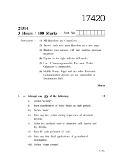

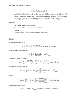


© Copyright 2026