
Introduction to computing with finite difference
Introduction to computing with finite difference
methods
Hans Petter Langtangen1,2
1
Center for Biomedical Computing, Simula Research Laboratory
2
Department of Informatics, University of Oslo
Mar 21, 2015
Contents
1 Finite difference methods
1.1 A basic model for exponential decay . . . . . .
1.2 The Forward Euler scheme . . . . . . . . . . .
1.3 The Backward Euler scheme . . . . . . . . . . .
1.4 The Crank-Nicolson scheme . . . . . . . . . . .
1.5 The unifying θ-rule . . . . . . . . . . . . . . . .
1.6 Constant time step . . . . . . . . . . . . . . . .
1.7 Compact operator notation for finite differences
.
.
.
.
.
.
.
.
.
.
.
.
.
.
.
.
.
.
.
.
.
.
.
.
.
.
.
.
.
.
.
.
.
.
.
.
.
.
.
.
.
.
.
.
.
.
.
.
.
.
.
.
.
.
.
.
.
.
.
.
.
.
.
.
.
.
.
.
.
.
.
.
.
.
.
.
.
.
.
.
.
.
.
.
.
.
.
.
.
.
.
.
.
.
.
.
.
.
.
.
.
.
.
.
.
.
.
.
.
.
.
.
.
.
.
.
.
.
.
.
.
.
.
.
.
.
5
5
6
9
10
12
13
13
2 Implementation
2.1 Making a solver function . . . . . . . . . . . . . . .
2.2 Verifying the implementation . . . . . . . . . . . .
2.3 Computing the numerical error as a mesh function
2.4 Computing the norm of the numerical error . . . .
2.5 Experiments with computing and plotting . . . . .
2.6 Memory-saving implementation . . . . . . . . . . .
.
.
.
.
.
.
.
.
.
.
.
.
.
.
.
.
.
.
.
.
.
.
.
.
.
.
.
.
.
.
.
.
.
.
.
.
.
.
.
.
.
.
.
.
.
.
.
.
.
.
.
.
.
.
.
.
.
.
.
.
.
.
.
.
.
.
.
.
.
.
.
.
.
.
.
.
.
.
.
.
.
.
.
.
.
.
.
.
.
.
.
.
.
.
.
.
.
.
.
.
.
.
15
16
22
23
24
26
30
.
.
.
.
.
.
.
3 Exercises
4 Analysis of finite difference equations
4.1 Experimental investigation of oscillatory solutions . . . .
4.2 Exact numerical solution . . . . . . . . . . . . . . . . . . .
4.3 Stability . . . . . . . . . . . . . . . . . . . . . . . . . . . .
4.4 Comparing amplification factors . . . . . . . . . . . . . .
4.5 Series expansion of amplification factors . . . . . . . . . .
4.6 The fraction of numerical and exact amplification factors
4.7 The global error at a point . . . . . . . . . . . . . . . . .
4.8 Integrated errors . . . . . . . . . . . . . . . . . . . . . . .
4.9 Truncation error . . . . . . . . . . . . . . . . . . . . . . .
4.10 Consistency, stability, and convergence . . . . . . . . . . .
32
.
.
.
.
.
.
.
.
.
.
.
.
.
.
.
.
.
.
.
.
.
.
.
.
.
.
.
.
.
.
.
.
.
.
.
.
.
.
.
.
.
.
.
.
.
.
.
.
.
.
.
.
.
.
.
.
.
.
.
.
.
.
.
.
.
.
.
.
.
.
.
.
.
.
.
.
.
.
.
.
.
.
.
.
.
.
.
.
.
.
.
.
.
.
.
.
.
.
.
.
.
.
.
.
.
.
.
.
.
.
.
.
.
.
.
.
.
.
.
.
.
.
.
.
.
.
.
.
.
.
34
36
38
39
40
40
43
43
43
44
46
5 Exercises
46
6 Model extensions
6.1 Generalization: including a variable coefficient .
6.2 Generalization: including a source term . . . . .
6.3 Implementation of the generalized model problem
6.4 Verifying a constant solution . . . . . . . . . . .
6.5 Verification via manufactured solutions . . . . . .
6.6 Computing convergence rates . . . . . . . . . . .
6.7 Extension to systems of ODEs . . . . . . . . . .
.
.
.
.
.
.
.
.
.
.
.
.
.
.
.
.
.
.
.
.
.
.
.
.
.
.
.
.
.
.
.
.
.
.
.
.
.
.
.
.
.
.
.
.
.
.
.
.
.
.
.
.
.
.
.
.
.
.
.
.
.
.
.
.
.
.
.
.
.
.
.
.
.
.
.
.
.
.
.
.
.
.
.
.
.
.
.
.
.
.
.
.
.
.
.
.
.
.
.
.
.
.
.
.
.
.
.
.
.
.
.
.
.
.
.
.
.
.
.
.
.
.
.
.
.
.
47
48
49
49
50
51
53
54
7 General first-order ODEs
7.1 Generic form of first-order ODEs . . . . . . . . . .
7.2 The θ-rule . . . . . . . . . . . . . . . . . . . . . . .
7.3 An implicit 2-step backward scheme . . . . . . . .
7.4 Leapfrog schemes . . . . . . . . . . . . . . . . . . .
7.5 The 2nd-order Runge-Kutta method . . . . . . . .
7.6 A 2nd-order Taylor-series method . . . . . . . . . .
7.7 The 2nd- and 3rd-order Adams-Bashforth schemes
7.8 The 4th-order Runge-Kutta method . . . . . . . .
7.9 The Odespy software . . . . . . . . . . . . . . . . .
7.10 Example: Runge-Kutta methods . . . . . . . . . .
7.11 Example: Adaptive Runge-Kutta methods . . . . .
.
.
.
.
.
.
.
.
.
.
.
.
.
.
.
.
.
.
.
.
.
.
.
.
.
.
.
.
.
.
.
.
.
.
.
.
.
.
.
.
.
.
.
.
.
.
.
.
.
.
.
.
.
.
.
.
.
.
.
.
.
.
.
.
.
.
.
.
.
.
.
.
.
.
.
.
.
.
.
.
.
.
.
.
.
.
.
.
.
.
.
.
.
.
.
.
.
.
.
.
.
.
.
.
.
.
.
.
.
.
.
.
.
.
.
.
.
.
.
.
.
.
.
.
.
.
.
.
.
.
.
.
.
.
.
.
.
.
.
.
.
.
.
.
.
.
.
.
.
.
.
.
.
.
.
.
.
.
.
.
.
.
.
.
.
.
.
.
.
.
.
.
.
.
.
.
.
.
.
.
.
.
.
.
.
.
.
55
55
55
56
56
57
57
57
58
59
60
62
8 Exercises
64
9 Applications of exponential decay models
9.1 Scaling . . . . . . . . . . . . . . . . . . . . .
9.2 Evolution of a population . . . . . . . . . .
9.3 Compound interest and inflation . . . . . .
9.4 Radioactive decay . . . . . . . . . . . . . .
9.5 Newton’s law of cooling . . . . . . . . . . .
9.6 Decay of atmospheric pressure with altitude
9.7 Compaction of sediments . . . . . . . . . .
9.8 Vertical motion of a body in a viscous fluid
9.9 Decay ODEs from solving a PDE by Fourier
10 Exercises
. . . . . . .
. . . . . . .
. . . . . . .
. . . . . . .
. . . . . . .
. . . . . . .
. . . . . . .
. . . . . . .
expansions
.
.
.
.
.
.
.
.
.
.
.
.
.
.
.
.
.
.
.
.
.
.
.
.
.
.
.
.
.
.
.
.
.
.
.
.
.
.
.
.
.
.
.
.
.
.
.
.
.
.
.
.
.
.
.
.
.
.
.
.
.
.
.
.
.
.
.
.
.
.
.
.
.
.
.
.
.
.
.
.
.
.
.
.
.
.
.
.
.
.
.
.
.
.
.
.
.
.
.
.
.
.
.
.
.
.
.
.
.
.
.
.
.
.
.
.
.
.
.
.
.
.
.
.
.
.
67
67
68
69
70
72
72
73
75
78
79
2
List of Exercises, Problems, and Projects
Exercise
Exercise
Exercise
Exercise
Exercise
Exercise
Exercise
Exercise
Exercise
Exercise
Exercise
Exercise
Problem
Problem
Exercise
Exercise
Exercise
Exercise
Exercise
Exercise
Exercise
Exercise
Exercise
Project
Exercise
Exercise
Exercise
Exercise
Exercise
Exercise
Exercise
1
2
3
4
5
6
7
8
9
10
11
12
13
14
15
16
17
18
19
20
21
22
23
24
25
26
27
28
29
30
31
Differentiate a function
Experiment with integer division
Experiment with wrong computations
Plot the error function
Change formatting of numbers and debug
Visualize the accuracy of finite differences
Explore the θ-rule for exponential ...
Experiment with precision in tests and the ...
Implement the 2-step backward scheme
Implement the 2nd-order Adams-Bashforth scheme ...
Implement the 3rd-order Adams-Bashforth scheme ...
Analyze explicit 2nd-order methods
Implement and investigate the Leapfrog scheme
Make a unified implementation of many schemes
Derive schemes for Newton’s law of cooling
Implement schemes for Newton’s law of cooling
Find time of murder from body temperature
Simulate an oscillating cooling process
Radioactive decay of Carbon-14
Simulate stochastic radioactive decay
Radioactive decay of two substances
Simulate the pressure drop in the atmosphere
Make a program for vertical motion in a fluid
Simulate parachuting
Formulate vertical motion in the atmosphere
Simulate vertical motion in the atmosphere
Compute y = |x| by solving an ODE
Simulate growth of a fortune with random interest ...
Simulate a population in a changing environment ...
Simulate logistic growth
Rederive the equation for continuous compound ...
3
p.
p.
p.
p.
p.
p.
p.
p.
p.
p.
p.
p.
p.
p.
p.
p.
p.
p.
p.
p.
p.
p.
p.
p.
p.
p.
p.
p.
p.
p.
p.
32
32
33
33
33
46
47
64
65
65
65
65
65
67
79
79
80
80
81
81
81
82
82
83
84
84
85
85
86
86
86
Finite difference methods for partial differential equations (PDEs) employ a range of concepts
and tools that can be introduced and illustrated in the context of simple ordinary differential
equation (ODE) examples. This is what we do in the present document. By first working with
ODEs, we keep the mathematical problems to be solved as simple as possible (but no simpler),
thereby allowing full focus on understanding the key concepts and tools. The choice of topics
in the forthcoming treatment of ODEs is therefore solely dominated by what carries over to
numerical methods for PDEs.
Theory and practice are primarily illustrated by solving the very simple ODE u0 = −au,
u(0) = I, where a > 0 is a constant, but we also address the generalized problem u0 = −a(t)u+b(t)
and the nonlinear problem u0 = f (u, t). The following topics are introduced:
• How to think when constructing finite difference methods, with special focus on the Forward
Euler, Backward Euler, and Crank-Nicolson (midpoint) schemes
• How to formulate a computational algorithm and translate it into Python code
• How to make curve plots of the solutions
• How to compute numerical errors
• How to compute convergence rates
• How to verify an implementation and automate verification through test functions in Python
• How to work with Python concepts such as arrays, lists, dictionaries, lambda functions,
functions in functions (closures)
• How to perform array computing and understand the difference from scalar computing
• How to uncover numerical artifacts in the computed solution
• How to analyze the numerical schemes mathematically to understand why artifacts occur
• How to derive mathematical expressions for various measures of the error in numerical
methods, frequently by using the sympy software for symbolic computation
• Introduce concepts such as finite difference operators, mesh (grid), mesh functions, stability,
truncation error, consistency, and convergence
• Present additional methods for the general nonlinear ODE u0 = f (u, t), which is either a
scalar ODE or a system of ODEs
• How to access professional packages for solving ODEs
• How the model equation u0 = −au arises in a wide range of phenomena in physics, biology,
and finance
The exposition in a nutshell.
Everything we cover is put into a practical, hands-on context. All mathematics is translated
into working computing codes, and all the mathematical theory of finite difference methods
presented here is motivated from a strong need to understand strange behavior of programs.
Two fundamental questions saturate the text:
• How to we solve a differential equation problem and produce numbers?
4
• How to we trust the answer?
1
Finite difference methods
Goal.
We explain the basic ideas of finite difference methods using a simple ordinary differential
equation u0 = −au as primary example. Emphasis is put on the reasoning when discretizing
the problem and introduction of key concepts such as mesh, mesh function, finite difference
approximations, averaging in a mesh, derivation of algorithms, and discrete operator
notation.
1.1
A basic model for exponential decay
Our model problem is perhaps the simplest ordinary differential equation (ODE):
u0 (t) = −au(t),
Here, a > 0 is a constant and u0 (t) means differentiation with respect to time t. This type of
equation arises in a number of widely different phenomena where some quantity u undergoes
exponential reduction. Examples include radioactive decay, population decay, investment decay,
cooling of an object, pressure decay in the atmosphere, and retarded motion in fluids (for some of
these models, a can be negative as well), see Section 9 for details and motivation. We have chosen
this particular ODE not only because its applications are relevant, but even more because studying
numerical solution methods for this simple ODE gives important insight that can be reused in
much more complicated settings, in particular when solving diffusion-type partial differential
equations.
The analytical solution of the ODE is found by the method of separation of variables, which
results in
u(t) = Ce−at ,
for any arbitrary constant C. To formulate a mathematical problem for which there is a unique
solution, we need a condition to fix the value of C. This condition is known as the initial condition
and stated as u(0) = I. That is, we know the value I of u when the process starts at t = 0. The
exact solution is then u(t) = Ie−at .
We seek the solution u(t) of the ODE for t ∈ (0, T ]. The point t = 0 is not included since we
know u here and assume that the equation governs u for t > 0. The complete ODE problem then
reads: find u(t) such that
u0 = −au, t ∈ (0, T ],
u(0) = I .
(1)
This is known as a continuous problem because the parameter t varies continuously from 0 to
T . For each t we have a corresponding u(t). There are hence infinitely many values of t and
u(t). The purpose of a numerical method is to formulate a corresponding discrete problem whose
solution is characterized by a finite number of values, which can be computed in a finite number
of steps on a computer.
5
1.2
The Forward Euler scheme
Solving an ODE like (1) by a finite difference method consists of the following four steps:
1. discretizing the domain,
2. fulfilling the equation at discrete time points,
3. replacing derivatives by finite differences,
4. formulating a recursive algorithm.
Step 1: Discretizing the domain.
of Nt + 1 points
The time domain [0, T ] is represented by a finite number
0 = t0 < t1 < t2 < · · · < tNt −1 < tNt = T .
(2)
The collection of points t0 , t1 , . . . , tNt constitutes a mesh or grid. Often the mesh points will be
uniformly spaced in the domain [0, T ], which means that the spacing tn+1 − tn is the same for all
n. This spacing is often denoted by ∆t, in this case tn = n∆t.
We seek the solution u at the mesh points: u(tn ), n = 1, 2, . . . , Nt . Note that u0 is already
known as I. A notational short-form for u(tn ), which will be used extensively, is un . More
precisely, we let un be the numerical approximation to the exact solution u(tn ) at t = tn . The
numerical approximation is a mesh function, here defined only at the mesh points. When we need
to clearly distinguish between the numerical and the exact solution, we often place a subscript e
on the exact solution, as in ue (tn ). Figure 1 shows the tn and un points for n = 0, 1, . . . , Nt = 7
as well as ue (t) as the dashed line. The goal of a numerical method for ODEs is to compute
the mesh function by solving a finite set of algebraic equations derived from the original ODE
problem.
Since finite difference methods produce solutions at the mesh points only, it is an open question
what the solution is between the mesh points. One can use methods for interpolation to compute
the value of u between mesh points. The simplest (and most widely used) interpolation method
is to assume that u varies linearly between the mesh points, see Figure 2. Given un and un+1 ,
the value of u at some t ∈ [tn , tn+1 ] is by linear interpolation
u(t) ≈ un +
un+1 − un
(t − tn ) .
tn+1 − tn
(3)
Step 2: Fulfilling the equation at discrete time points. The ODE is supposed to hold for
all t ∈ (0, T ], i.e., at an infinite number of points. Now we relax that requirement and require that
the ODE is fulfilled at a finite set of discrete points in time. The mesh points t0 , t1 , . . . , tNt are a
natural (but not the only) choice of points. The original ODE is then reduced to the following
Nt equations:
u0 (tn ) = −au(tn ),
6
n = 0, . . . , Nt .
(4)
u
u2
u5
u3
u4
u1
u0
t0
t1
t2
t3
t4
t5
t
Figure 1: Time mesh with discrete solution values.
Step 3: Replacing derivatives by finite differences. The next and most essential step of
the method is to replace the derivative u0 by a finite difference approximation. Let us first try a
one-sided difference approximation (see Figure 3),
u0 (tn ) ≈
un+1 − un
.
tn+1 − tn
(5)
Inserting this approximation in (4) results in
un+1 − un
= −aun ,
tn+1 − tn
n = 0, 1, . . . , Nt − 1 .
(6)
Later it will be absolutely clear that if we want to compute the solution up to time level Nt , we
only need (4) to hold for n = 0, . . . , Nt − 1 since (6) for n = Nt − 1 creates an equation for the
final value uNt .
Equation (6) is the discrete counterpart to the original ODE problem (1), and often referred
to as finite difference scheme or more generally as the discrete equations of the problem. The
fundamental feature of these equations is that they are algebraic and can hence be straightforwardly
solved to produce the mesh function, i.e., the values of u at the mesh points (un , n = 1, 2, . . . , Nt ).
Step 4: Formulating a recursive algorithm. The final step is to identify the computational
algorithm to be implemented in a program. The key observation here is to realize that (6) can be
used to compute un+1 if un is known. Starting with n = 0, u0 is known since u0 = u(0) = I, and
7
u
u2
u5
u3
u4
u1
u0
t0
Figure 2:
solution).
t1
t2
t3
t4
t5
t
Linear interpolation between the discrete solution values (dashed curve is exact
(6) gives an equation for u1 . Knowing u1 , u2 can be found from (6). In general, un in (6) can be
assumed known, and then we can easily solve for the unknown un+1 :
un+1 = un − a(tn+1 − tn )un .
(7)
We shall refer to (7) as the Forward Euler (FE) scheme for our model problem. From a
mathematical point of view, equations of the form (7) are known as difference equations since
they express how differences in u, like un+1 − un , evolve with n. The finite difference method can
be viewed as a method for turning a differential equation into a difference equation.
Computation with (7) is straightforward:
u0 = I,
u1 = u0 − a(t1 − t0 )u0 = I(1 − a(t1 − t0 )),
u2 = u1 − a(t2 − t1 )u1 = I(1 − a(t1 − t0 ))(1 − a(t2 − t1 )),
u3 = u2 − a(t3 − t2 )u2 = I(1 − a(t1 − t0 ))(1 − a(t2 − t1 ))(1 − a(t3 − t2 )),
and so on until we reach uNt . Very often, tn+1 − tn is constant for all n, so we can introduce the
common symbol ∆t for the time step: ∆t = tn+1 − tn , n = 0, 1, . . . , Nt − 1. Using a constant
time step ∆t in the above calculations gives
8
u(t)
forward
tn−1
tn
tn +1
Figure 3: Illustration of a forward difference.
u0 = I,
u1 = I(1 − a∆t),
u2 = I(1 − a∆t)2 ,
u3 = I(1 − a∆t)3 ,
..
.
uNt = I(1 − a∆t)Nt .
This means that we have found a closed formula for un , and there is no need to let a computer
generate the sequence u1 , u2 , u3 , . . .. However, finding such a formula for un is possible only for a
few very simple problems, so in general finite difference equations must be solved on a computer.
As the next sections will show, the scheme (7) is just one out of many alternative finite
difference (and other) methods for the model problem (1).
1.3
The Backward Euler scheme
There are several choices of difference approximations in step 3 of the finite difference method as
presented in the previous section. Another alternative is
u0 (tn ) ≈
un − un−1
.
tn − tn−1
(8)
Since this difference is based on going backward in time (tn−1 ) for information, it is known as
the Backward Euler difference. Figure 4 explains the idea.
9
u(t)
backward
tn−1
tn
tn +1
Figure 4: Illustration of a backward difference.
Inserting (8) in (4) yields the Backward Euler (BE) scheme:
un − un−1
= −aun .
tn − tn−1
(9)
We assume, as explained under step 4 in Section 1.2, that we have computed u0 , u1 , . . . , un−1
such that (9) can be used to compute un . For direct similarity with the Forward Euler scheme
(7) we replace n by n + 1 in (9) and solve for the unknown value un+1 :
un+1 =
1.4
1
1 + a(tn+1 − tn )
un .
(10)
The Crank-Nicolson scheme
The finite difference approximations used to derive the schemes (7) and (10) are both one-sided
differences, known to be less accurate than central (or midpoint) differences. We shall now
construct a central difference at tn+ 21 = 12 (tn + tn+1 ), or tn+ 12 = (n + 12 )∆t if the mesh spacing is
uniform in time. The approximation reads
u0 (tn+ 21 ) ≈
un+1 − un
.
tn+1 − tn
(11)
Note that the fraction on the right-hand side is the same as for the Forward Euler approximation
(5) and the Backward Euler approximation (8) (with n replaced by n + 1). The accuracy of this
fraction as an approximation to the derivative of u depends on where we seek the derivative: in
the center of the interval [tn , tn+1 ] or at the end points.
With the formula (11), where u0 is evaluated at tn+ 12 , it is natural to demand the ODE to be
fulfilled at the time points between the mesh points:
10
u(t)
centered
tn
tn +12
tn +1
Figure 5: Illustration of a centered difference.
u0 (tn+ 21 ) = −au(tn+ 12 ),
n = 0, . . . , Nt − 1 .
(12)
Using (11) in (12) results in
1
un+1 − un
= −aun+ 2 ,
tn+1 − tn
(13)
1
where un+ 2 is a short form for u(tn+ 12 ). The problem is that we aim to compute un for integer n,
1
implying that un+ 2 is not a quantity computed by our method. It must therefore be expressed
by the quantities that we actually produce, i.e., the numerical solution at the mesh points. One
1
possibility is to approximate un+ 2 as an arithmetic mean of the u values at the neighboring mesh
points:
1
un+ 2 ≈
1 n
(u + un+1 ) .
2
(14)
Using (14) in (13) results in
un+1 − un
1
= −a (un + un+1 ) .
(15)
tn+1 − tn
2
Figure 5 sketches the geometric interpretation of such a centered difference.
We assume that un is already computed so that un+1 is the unknown, which we can solve for:
un+1 =
1 − 12 a(tn+1 − tn ) n
u .
1 + 12 a(tn+1 − tn )
(16)
The finite difference scheme (16) is often called the Crank-Nicolson (CN) scheme or a midpoint
or centered scheme.
11
1.5
The unifying θ-rule
The Forward Euler, Backward Euler, and Crank-Nicolson schemes can be formulated as one
scheme with a varying parameter θ:
un+1 − un
= −a(θun+1 + (1 − θ)un ) .
tn+1 − tn
(17)
Observe:
• θ = 0 gives the Forward Euler scheme
• θ = 1 gives the Backward Euler scheme, and
• θ=
1
2
gives the Crank-Nicolson scheme.
• We may alternatively choose any other value of θ in [0, 1].
As before, un is considered known and un+1 unknown, so we solve for the latter:
un+1 =
1 − (1 − θ)a(tn+1 − tn )
.
1 + θa(tn+1 − tn )
(18)
This scheme is known as the θ-rule, or alternatively written as the "theta-rule".
Derivation.
We start with replacing u0 by the fraction
un+1 − un
,
tn+1 − tn
in the Forward Euler, Backward Euler, and Crank-Nicolson schemes. Then we observe that
the difference between the methods concerns which point this fraction approximates the
derivative. Or in other words, at which point we sample the ODE. So far this has been the
end points or the midpoint of [tn , tn+1 ]. However, we may choose any point t˜ ∈ [tn , tn+1 ].
The difficulty is that evaluating the right-hand side −au at an arbitrary point faces the same
problem as in Section 1.4: the point value must be expressed by the discrete u quantities
that we compute by the scheme, i.e., un and un+1 . Following the averaging idea from
Section 1.4, the value of u at an arbitrary point t˜ can be calculated as a weighted average,
which generalizes the arithmetic mean 12 un + 12 un+1 . If we express t˜ as a weighted average
tn+θ = θtn+1 + (1 − θ)tn ,
where θ ∈ [0, 1] is the weighting factor, we can write
u(t˜) = u(θtn+1 + (1 − θ)tn ) ≈ θun+1 + (1 − θ)un .
(19)
We can now let the ODE hold at the point t˜ ∈ [tn , tn+1 ], approximate u0 by the fraction
(u
− un )/(tn+1 − tn ), and approximate the right-hand side −au by the weighted average
(19). The result is (17).
n+1
12
1.6
Constant time step
All schemes up to now have been formulated for a general non-uniform mesh in time: t0 , t1 , . . . , tNt .
Non-uniform meshes are highly relevant since one can use many points in regions where u varies
rapidly, and save points in regions where u is slowly varying. This is the key idea of adaptive
methods where the spacing of the mesh points are determined as the computations proceed.
However, a uniformly distributed set of mesh points is very common and sufficient for many
applications. It therefore makes sense to present the finite difference schemes for a uniform point
distribution tn = n∆t, where ∆t is the constant spacing between the mesh points, also referred
to as the time step. The resulting formulas look simpler and are perhaps more well known.
Summary of schemes for constant time step.
un+1 = (1 − a∆t)un
Forward Euler
1
un
un+1 =
Backward Euler
1 + a∆t
1 − 12 a∆t n
u
Crank-Nicolson
un+1 =
1 + 12 a∆t
1 − (1 − θ)a∆t n
un+1 =
u
The θ − rule
1 + θa∆t
(20)
(21)
(22)
(23)
Not surprisingly, we present these three alternative schemes because they have different pros
and cons, both for the simple ODE in question (which can easily be solved as accurately as
desired), and for more advanced differential equation problems.
Test the understanding.
At this point it can be good training to apply the explained finite difference discretization
techniques to a slightly different equation. Exercise 15 is therefore highly recommended to
check that the key concepts are understood.
1.7
Compact operator notation for finite differences
Finite difference formulas can be tedious to write and read, especially for differential equations
with many terms and many derivatives. To save space and help the reader of the scheme to
quickly see the nature of the difference approximations, we introduce a compact notation. A
forward difference approximation is denoted by the Dt+ operator:
un+1 − un
d
≈ u(tn ) .
(24)
∆t
dt
The notation consists of an operator that approximates differentiation with respect to an independent variable, here t. The operator is built of the symbol D, with the variable as subscript and a
superscript denoting the type of difference. The superscript + indicates a forward difference. We
place square brackets around the operator and the function it operates on and specify the mesh
point, where the operator is acting, by a superscript.
[Dt+ u]n =
13
The corresponding operator notation for a centered difference and a backward difference reads
1
1
un+ 2 − un− 2
d
[Dt u] =
≈ u(tn ),
∆t
dt
n
and
(25)
d
un − un−1
≈ u(tn ) .
(26)
∆t
dt
denotes the backward difference, while no superscript implies a
[Dt− u]n =
Note that the superscript −
central difference.
An averaging operator is also convenient to have:
1
1 n− 1
(u 2 + un+ 2 ) ≈ u(tn )
(27)
2
The superscript t indicates that the average is taken along the time coordinate. The common
1
average (un + un+1 )/2 can now be expressed as [ut ]n+ 2 . (When also spatial coordinates enter
the problem, we need the explicit specification of the coordinate after the bar.)
The Backward Euler finite difference approximation to u0 = −au can be written as follows
utilizing the compact notation:
[ut ]n =
[Dt− u]n = −aun .
In difference equations we often place the square brackets around the whole equation, to indicate
at which mesh point the equation applies, since each term is supposed to be approximated at the
same point:
[Dt− u = −au]n .
(28)
The Forward Euler scheme takes the form
[Dt+ u = −au]n ,
(29)
while the Crank-Nicolson scheme is written as
1
[Dt u = −aut ]n+ 2 .
(30)
Question.
Apply (25) and (27) and write out the expressions to see that (30) is indeed the CrankNicolson scheme.
The θ-rule can be specified by
¯ t u = −aut,θ ]n+θ ,
[D
(31)
if we define a new time difference
¯ t u]n+θ =
[D
un+1 − un
,
tn+1 − tn
and a weighted averaging operator
14
(32)
[ut,θ ]n+θ = (1 − θ)un + θun+1 ≈ u(tn+θ ),
(33)
where θ ∈ [0, 1]. Note that for θ = 12 we recover the standard centered difference and the standard
arithmetic mean. The idea in (31) is to sample the equation at tn+θ , use a skew difference at
¯ t u]n+θ , and a skew mean value. An alternative notation is
that point [D
1
[Dt u]n+ 2 = θ[−au]n+1 + (1 − θ)[−au]n .
Looking at the various examples above and comparing them with the underlying differential
equations, we see immediately which difference approximations that have been used and at which
point they apply. Therefore, the compact notation effectively communicates the reasoning behind
turning a differential equation into a difference equation.
2
Implementation
Goal.
We want make a computer program for solving
u0 (t) = −au(t),
t ∈ (0, T ],
u(0) = I,
by finite difference methods. The program should also display the numerical solution as a
curve on the screen, preferably together with the exact solution.
All programs referred to in this section are found in the src/decay1 directory (we use the
classical Unix term directory for what many others nowadays call folder).
Mathematical problem. We want to explore the Forward Euler scheme, the Backward Euler,
and the Crank-Nicolson schemes applied to our model problem. From an implementational point
of view, it is advantageous to implement the θ-rule
un+1 =
1 − (1 − θ)a∆t n
u ,
1 + θa∆t
since it can generate the three other schemes by various of choices of θ: θ = 0 for Forward Euler,
θ = 1 for Backward Euler, and θ = 1/2 for Crank-Nicolson. Given a, u0 = I, T , and ∆t, our task
is to use the θ-rule to compute u1 , u2 , . . . , uNt , where tNt = Nt ∆t, and Nt the closest integer to
T /∆t.
Computer Language: Python. Any programming language can be used to generate the
un+1 values from the formula above. However, in this document we shall mainly make use of
Python of several reasons:
• Python has a very clean, readable syntax (often known as "executable pseudo-code").
• Python code is very similar to MATLAB code (and MATLAB has a particularly widespread
use for scientific computing).
1 http://tinyurl.com/nm5587k/decay
15
• Python is a full-fledged, very powerful programming language.
• Python is similar to, but much simpler to work with and results in more reliable code than
C++.
• Python has a rich set of modules for scientific computing, and its popularity in scientific
computing is rapidly growing.
• Python was made for being combined with compiled languages (C, C++, Fortran) to
reuse existing numerical software and to reach high computational performance of new
implementations.
• Python has extensive support for administrative task needed when doing large-scale computational investigations.
• Python has extensive support for graphics (visualization, user interfaces, web applications).
• FEniCS, a very powerful tool for solving PDEs by the finite element method, is most
human-efficient to operate from Python.
Learning Python is easy. Many newcomers to the language will probably learn enough from the
forthcoming examples to perform their own computer experiments. The examples start with
simple Python code and gradually make use of more powerful constructs as we proceed. As long
as it is not inconvenient for the problem at hand, our Python code is made as close as possible to
MATLAB code for easy transition between the two languages.
Readers who feel the Python examples are too hard to follow will probably benefit from
reading a tutorial, e.g.,
• The Official Python Tutorial2
• Python Tutorial on tutorialspoint.com3
• Interactive Python tutorial site4
• A Beginner’s Python Tutorial5
The author also has a comprehensive book [4] that teaches scientific programming with Python
from the ground up.
2.1
Making a solver function
We choose to have an array u for storing the un values, n = 0, 1, . . . , Nt . The algorithmic steps
are
1. initialize u0
2. for t = tn , n = 1, 2, . . . , Nt : compute un using the θ-rule formula
2 http://docs.python.org/2/tutorial/
3 http://www.tutorialspoint.com/python/
4 http://www.learnpython.org/
5 http://en.wikibooks.org/wiki/A_Beginner’s_Python_Tutorial
16
Function for computing the numerical solution. The following Python function takes the
input data of the problem (I, a, T , ∆t, θ) as arguments and returns two arrays with the solution
u0 , . . . , uNt and the mesh points t0 , . . . , tNt , respectively:
from numpy import *
def solver(I, a, T, dt, theta):
"""Solve u’=-a*u, u(0)=I, for t in (0,T] with steps of dt."""
Nt = int(T/dt)
# no of time intervals
T = Nt*dt
# adjust T to fit time step dt
u = zeros(Nt+1)
# array of u[n] values
t = linspace(0, T, Nt+1) # time mesh
u[0] = I
# assign initial condition
for n in range(0, Nt):
# n=0,1,...,Nt-1
u[n+1] = (1 - (1-theta)*a*dt)/(1 + theta*dt*a)*u[n]
return u, t
The numpy library contains a lot of functions for array computing. Most of the function names
are similar to what is found in the alternative scientific computing language MATLAB. Here we
make use of
• zeros(Nt+1) for creating an array of a size Nt+1 and initializing the elements to zero
• linspace(0, T, Nt+1) for creating an array with Nt+1 coordinates uniformly distributed
between 0 and T
The for loop deserves a comment, especially for newcomers to Python. The construction
range(0, Nt, s) generates all integers from 0 to Nt in steps of s, but not including Nt. Omitting
s means s=1. For example, range(0, 6, 3) gives 0 and 3, while range(0, Nt) generates 0, 1,
..., Nt-1. Our loop implies the following assignments to u[n+1]: u[1], u[2], ..., u[Nt], which is
what we want since u has length Nt+1. The first index in Python arrays or lists is always 0 and
the last is then len(u)-1. The length of an array u is obtained by len(u) or u.size.
To compute with the solver function, we need to call it. Here is a sample call:
u, t = solver(I=1, a=2, T=8, dt=0.8, theta=1)
Integer division. The shown implementation of the solver may face problems and wrong
results if T, a, dt, and theta are given as integers, see Exercises 2 and 3. The problem is
related to integer division in Python (as well as in Fortran, C, C++, and many other computer
languages): 1/2 becomes 0, while 1.0/2, 1/2.0, or 1.0/2.0 all become 0.5. It is enough that at
least the nominator or the denominator is a real number (i.e., a float object) to ensure correct
mathematical division. Inserting a conversion dt = float(dt) guarantees that dt is float and
avoids problems in Exercise 3.
Another problem with computing Nt = T /∆t is that we should round Nt to the nearest
integer. With Nt = int(T/dt) the int operation picks the largest integer smaller than T/dt.
Correct mathematical rounding as known from school is obtained by
Nt = int(round(T/dt))
The complete version of our improved, safer solver function then becomes
17
from numpy import *
def solver(I, a, T, dt, theta):
"""Solve u’=-a*u, u(0)=I, for t in (0,T] with steps of dt."""
dt = float(dt)
# avoid integer division
Nt = int(round(T/dt))
# no of time intervals
T = Nt*dt
# adjust T to fit time step dt
u = zeros(Nt+1)
# array of u[n] values
t = linspace(0, T, Nt+1) # time mesh
u[0] = I
# assign initial condition
for n in range(0, Nt):
# n=0,1,...,Nt-1
u[n+1] = (1 - (1-theta)*a*dt)/(1 + theta*dt*a)*u[n]
return u, t
Doc strings. Right below the header line in the solver function there is a Python string
enclosed in triple double quotes """. The purpose of this string object is to document what the
function does and what the arguments are. In this case the necessary documentation do not span
more than one line, but with triple double quoted strings the text may span several lines:
def solver(I, a, T, dt, theta):
"""
Solve
u’(t) = -a*u(t),
with initial condition u(0)=I, for t in the time interval
(0,T]. The time interval is divided into time steps of
length dt.
theta=1 corresponds to the Backward Euler scheme, theta=0
to the Forward Euler scheme, and theta=0.5 to the CrankNicolson method.
"""
...
Such documentation strings appearing right after the header of a function are called doc strings.
There are tools that can automatically produce nicely formatted documentation by extracting
the definition of functions and the contents of doc strings.
It is strongly recommended to equip any function whose purpose is not obvious with a doc
string. Nevertheless, the forthcoming text deviates from this rule if the function is explained in
the text.
Formatting of numbers. Having computed the discrete solution u, it is natural to look at
the numbers:
# Write out a table of t and u values:
for i in range(len(t)):
print t[i], u[i]
This compact print statement gives unfortunately quite ugly output because the t and u values
are not aligned in nicely formatted columns. To fix this problem, we recommend to use the printf
format, supported most programming languages inherited from C. Another choice is Python’s
recent format string syntax.
Writing t[i] and u[i] in two nicely formatted columns is done like this with the printf
format:
18
print ’t=%6.3f u=%g’ % (t[i], u[i])
The percentage signs signify "slots" in the text where the variables listed at the end of the
statement are inserted. For each "slot" one must specify a format for how the variable is going to
appear in the string: s for pure text, d for an integer, g for a real number written as compactly
as possible, 9.3E for scientific notation with three decimals in a field of width 9 characters (e.g.,
-1.351E-2), or .2f for standard decimal notation with two decimals formatted with minimum
width. The printf syntax provides a quick way of formatting tabular output of numbers with full
control of the layout.
The alternative format string syntax looks like
print ’t={t:6.3f} u={u:g}’.format(t=t[i], u=u[i])
As seen, this format allows logical names in the "slots" where t[i] and u[i] are to be inserted.
The "slots" are surrounded by curly braces, and the logical name is followed by a colon and then
the printf-like specification of how to format real numbers, integers, or strings.
Running the program. The function and main program shown above must be placed in a
file, say with name decay_v1.py6 (v1 for 1st version of this program). Make sure you write the
code with a suitable text editor (Gedit, Emacs, Vim, Notepad++, or similar). The program is
run by executing the file this way:
Terminal> python decay_v1.py
The text Terminal> just indicates a prompt in a Unix/Linux or DOS terminal window. After this
prompt, which will look different in your terminal window, depending on the terminal application
and how it is set up, commands like python decay_v1.py can be issued. These commands are
interpreted by the operating system.
We strongly recommend to run Python programs within the IPython shell. First start IPython
by typing ipython in the terminal window. Inside the IPython shell, our program decay_v1.py
is run by the command run decay_v1.py:
Terminal> ipython
In
t=
t=
t=
t=
t=
t=
t=
t=
t=
t=
t=
[1]: run decay_v1.py
0.000 u=1
0.800 u=0.384615
1.600 u=0.147929
2.400 u=0.0568958
3.200 u=0.021883
4.000 u=0.00841653
4.800 u=0.00323713
5.600 u=0.00124505
6.400 u=0.000478865
7.200 u=0.000184179
8.000 u=7.0838e-05
In [2]:
6 http://tinyurl.com/nm5587k/decay/decay_v1.py
19
The advantage of running programs in IPython are many: previous commands are easily
recalled with the up arrow, %pdb turns on debugging so that variables can be examined if the
program aborts due to an exception, output of commands are stored in variables, programs and
statements can be profiled, any operating system command can be executed, modules can be
loaded automatically and other customizations can be performed when starting IPython – to
mention a few of the most useful features.
Although running programs in IPython is strongly recommended, most execution examples in
the forthcoming text use the standard Python shell with prompt >>> and run programs through
a typesetting like
Terminal> python programname
The reason is that such typesetting makes the text more compact in the vertical direction than
showing sessions with IPython syntax.
Plotting the solution. Having the t and u arrays, the approximate solution u is visualized
by the intuitive command plot(t, u):
from matplotlib.pyplot import *
plot(t, u)
show()
It will be illustrative to also plot ue (t) for comparison. We first need to make a function for
computing the analytical solution ue (t) = Ie−at of the model problem:
def exact_solution(t, I, a):
return I*exp(-a*t)
It is tempting to just do
u_e = exact_solution(t, I, a)
plot(t, u, t, u_e)
However, this is not exactly what we want: the plot function draws straight lines between the
discrete points (t[n], u_e[n]) while ue (t) varies as an exponential function between the mesh
points. The technique for showing the “exact” variation of ue (t) between the mesh points is to
introduce a very fine mesh for ue (t):
t_e = linspace(0, T, 1001)
# fine mesh
u_e = exact_solution(t_e, I, a)
We can also plot the curves with different colors and styles, e.g.,
plot(t_e, u_e, ’b-’,
t,
u,
’r--o’)
# blue line for u_e
# red dashes w/circles
With more than one curve in the plot we need to associate each curve with a legend. We
also want appropriate names on the axis, a title, and a file containing the plot as an image for
inclusion in reports. The Matplotlib package (matplotlib.pyplot) contains functions for this
purpose. The names of the functions are similar to the plotting functions known from MATLAB.
A complete function for creating the comparison plot becomes
20
theta=1, dt=0.8
1.0
numerical
exact
0.8
u
0.6
0.4
0.2
0.0
0
1
2
3
4
t
5
6
7
8
Figure 6: Comparison of numerical and exact solution.
from matplotlib.pyplot import *
def plot_numerical_and_exact(theta, I, a, T, dt):
"""Compare the numerical and exact solution in a plot."""
u, t = solver(I=I, a=a, T=T, dt=dt, theta=theta)
t_e = linspace(0, T, 1001)
u_e = exact_solution(t_e, I, a)
# fine mesh for u_e
plot(t,
u,
’r--o’,
# red dashes w/circles
t_e, u_e, ’b-’)
# blue line for exact sol.
legend([’numerical’, ’exact’])
xlabel(’t’)
ylabel(’u’)
title(’theta=%g, dt=%g’ % (theta, dt))
savefig(’plot_%s_%g.png’ % (theta, dt))
plot_numerical_and_exact(I=1, a=2, T=8, dt=0.8, theta=1)
show()
Note that savefig here creates a PNG file whose name reflects the values of θ and ∆t so that we
can easily distinguish files from different runs with θ and ∆t.
The complete code is found in the file decay_v2.py7 . The resulting plot is shown in Figure 6.
As seen, there is quite some discrepancy between the exact and the numerical solution. Fortunately,
the numerical solution approaches the exact one as ∆t is reduced.
7 http://tinyurl.com/nm5587k/decay/decay_v2.py
21
2.2
Verifying the implementation
It is easy to make mistakes while deriving and implementing numerical algorithms, so we should
never believe in the solution before it has been thoroughly verified. The most obvious idea to
verify the computations is to compare the numerical solution with the exact solution, when
that exists, but there will always be a discrepancy between these two solutions because of the
numerical approximations. The challenging question is whether we have the mathematically
correct discrepancy or if we have another, maybe small, discrepancy due to both an approximation
error and an error in the implementation. When looking at Figure 6, it is impossible to judge
whether the program is correct or not.
The purpose of verifying a program is to bring evidence for the property that there are no
errors in the implementation. To avoid mixing unavoidable approximation errors and undesired
implementation errors, we should try to make tests where we have some exact computation of
the discrete solution or at least parts of it. Examples will show how this can be done.
Running a few algorithmic steps by hand. The simplest approach to produce a correct
non-trivial reference solution for the discrete solution u of finite difference equations is to compute
a few steps of the algorithm by hand. Then we can compare the hand calculations with numbers
produced by the program.
A straightforward approach is to use a calculator and compute u1 , u2 , and u3 . With I = 0.1,
θ = 0.8, and ∆t = 0.8 we get
A≡
1 − (1 − θ)a∆t
= 0.298245614035
1 + θa∆t
u1 = AI = 0.0298245614035,
u2 = Au1 = 0.00889504462912,
u3 = Au2 = 0.00265290804728
Comparison of these manual calculations with the result of the solver function is carried out
in the function
def test_solver_three_steps():
"""Compare three steps with known manual computations."""
theta = 0.8; a = 2; I = 0.1; dt = 0.8
u_by_hand = array([I,
0.0298245614035,
0.00889504462912,
0.00265290804728])
Nt = 3 # number of time steps
u, t = solver(I=I, a=a, T=Nt*dt, dt=dt, theta=theta)
tol = 1E-15 # tolerance for comparing floats
diff = abs(u - u_by_hand).max()
success = diff <= tol
assert success
The test_solver_three_steps function follows widely used conventions for unit testing. By
following such conventions we can at a later stage easily execute a big test suite for our software.
The conventions are three-fold:
• The test function starts with test_ and takes no arguments.
22
• The test ends up in a boolean expression that is True if the test passed and False if it
failed.
• The function runs assert on the boolean expression, resulting in program abortion (due to
an AssertionError exception) if the test failed.
The main program can routinely run the verification test prior to solving the real problem:
test_solver_three_steps()
plot_numerical_and_exact(I=1, a=2, T=8, dt=0.8, theta=1)
show()
(Rather than calling test_*() functions explicitly, one will normally ask a testing framework like
nose or pytest to find and run such functions.) The complete program including the verification
above is found in the file decay_v3.py8 .
2.3
Computing the numerical error as a mesh function
Now that we have some evidence for a correct implementation, we are in a position to compare
the computed un values in the u array with the exact u values at the mesh points, in order to
study the error in the numerical solution.
A natural way to compare the exact and discrete solutions is to calculate their difference as a
mesh function:
en = ue (tn ) − un ,
n = 0, 1, . . . , Nt .
(34)
n
We may view ue = ue (tn ) as the representation of ue (t) as a mesh function rather than a
continuous function defined for all t ∈ [0, T ] (une is often called the representative of ue on the
mesh). Then, en = une − un is clearly the difference of two mesh functions. This interpretation of
en is natural when programming.
The error mesh function en can be computed by
u, t = solver(I, a, T, dt, theta)
u_e = exact_solution(t, I, a)
e = u_e - u
# Numerical sol.
# Representative of exact sol.
Note that the mesh functions u and u_e are represented by arrays and associated with the points
in the array t.
Array arithmetics.
The last statements
u_e = exact_solution(t, I, a)
e = u_e - u
are primary examples of array arithmetics: t is an array of mesh points that we pass to
exact_solution. This function evaluates -a*t, which is a scalar times an array, meaning
that the scalar is multiplied with each array element. The result is an array, let us call it
tmp1. Then exp(tmp1) means applying the exponential function to each element in tmp,
resulting an array, say tmp2. Finally, I*tmp2 is computed (scalar times array) and u_e refers
8 http://tinyurl.com/nm5587k/decay/decay_v3.py
23
to this array returned from exact_solution. The expression u_e - u is the difference
between two arrays, resulting in a new array referred to by e.
2.4
Computing the norm of the numerical error
Instead of working with the error en on the entire mesh, we often want one number expressing
the size of the error. This is obtained by taking the norm of the error function.
Let us first define norms of a function f (t) defined for all t ∈ [0, T ]. Three common norms are
!1/2
T
Z
2
||f ||L2 =
f (t) dt
,
(35)
0
T
Z
||f ||L1 =
|f (t)|dt,
(36)
||f ||L∞ = max |f (t)| .
(37)
0
t∈[0,T ]
The L2 norm (35) ("L-two norm") has nice mathematical properties and is the most popular
norm. It is a generalization of the well-known Eucledian norm of vectors to functions. The L∞ is
also called the max norm or the supremum norm. In fact, there is a whole family of norms,
!1/p
T
Z
f (t)p dt
||f ||Lp =
,
(38)
0
with p real. In particular, p = 1 corresponds to the L1 norm above while p = ∞ is the L∞ norm.
Numerical computations involving mesh functions need corresponding norms. Given a set of
function values, f n , and some associated mesh points, tn , a numerical integration rule can be used
to calculate the L2 and L1 norms defined above. Imagining that the mesh function is extended
to vary linearly between the mesh points, the Trapezoidal rule is in fact an exact integration rule.
A possible modification of the L2 norm for a mesh function f n on a uniform mesh with spacing
∆t is therefore the well-known Trapezoidal integration formula
||f n || =
∆t
N
t −1
X
1 0 2 1 Nt 2
(f ) + (f ) +
(f n )2
2
2
n=1
!!1/2
A common approximation of this expression, motivated by the convenience of having a simpler
formula, is
||f n ||`2 =
∆t
Nt
X
!1/2
(f n )2
.
n=0
This is called the discrete L2 norm and denoted by `2 . The error in ||f ||2`2 compared with the
Trapezoidal integration formula is ∆t((f 0 )2 + (f Nt )2 )/2, which means perturbed weights at the
end points of the mesh function, and the error goes to zero as ∆t → 0. As long as we are
consistent and stick to one kind of integration rule for the norm of a mesh function, the details
and accuracy of this rule is not of concern.
The three discrete norms for a mesh function f n , corresponding to the L2 , L1 , and L∞ norms
of f (t) defined above, are defined by
24
n
||f ||`2
∆t
Nt
X
!1/2
n 2
(f )
,
(39)
n=0
||f n ||`1 ∆t
Nt
X
|f n |
(40)
n=0
||f n ||`∞ max |f n | .
(41)
0≤n≤Nt
Note that the L2 , L1 , `2 , and `1 norms depend
on the length of the interval of interest (think
√
of f = 1, then the norms are proportional to T or T ). In some applications it is convenient to
think of a mesh function as just a vector of function values and neglect the information of the
mesh points. Then we can replace ∆t by T /Nt and drop T . Moreover, it is convenient to divide
by the total length of the vector, Nt + 1, instead of Nt . This reasoning gives rise to the vector
norms for a vector f = (f0 , . . . , fN ):
||f ||2 =
N
1 X
(fn )2
N + 1 n=0
!1/2
N
1 X
|fn |
||f ||1 =
N + 1 n=0
||f ||`∞ = max |fn | .
0≤n≤N
,
(42)
(43)
(44)
Here we have used the common vector component notation with subscripts (fn ) and N as length.
We will mostly work with mesh functions and use the discrete `2 norm (39) or the max norm `∞
(41), but the corresponding vector norms (42)-(44) are also much used in numerical computations,
so it is important to know the different norms and the relations between them.
A single number that expresses the size of the numerical error will be taken as ||en ||`2 and
called E:
v
u
Nt
u X
E = t∆t
(en )2
(45)
n=0
The corresponding Python code, using array arithmetics, reads
E = sqrt(dt*sum(e**2))
The sum function comes from numpy and computes the sum of the elements of an array. Also the
sqrt function is from numpy and computes the square root of each element in the array argument.
Scalar computing. Instead of doing array computing sqrt(dt*sum(e**2)) we can compute
with one element at a time:
m =
u_e
t =
for
len(u)
# length of u array (alt: u.size)
= zeros(m)
0
i in range(m):
25
u_e[i] = exact_solution(t, a, I)
t = t + dt
e = zeros(m)
for i in range(m):
e[i] = u_e[i] - u[i]
s = 0 # summation variable
for i in range(m):
s = s + e[i]**2
error = sqrt(dt*s)
Such element-wise computing, often called scalar computing, takes more code, is less readable,
and runs much slower than what we can achieve with array computing.
2.5
Experiments with computing and plotting
Let us wrap up the computation of the error measure and all the plotting statements for comparing
the exact and numerical solution in a new function explore. This function can be called for
various θ and ∆t values to see how the error varies with the method and the mesh resolution:
def explore(I, a, T, dt, theta=0.5, makeplot=True):
"""
Run a case with the solver, compute error measure,
and plot the numerical and exact solutions (if makeplot=True).
"""
u, t = solver(I, a, T, dt, theta)
# Numerical solution
u_e = exact_solution(t, I, a)
e = u_e - u
E = sqrt(dt*sum(e**2))
if makeplot:
figure()
# create new plot
t_e = linspace(0, T, 1001)
# fine mesh for u_e
u_e = exact_solution(t_e, I, a)
plot(t,
u,
’r--o’)
# red dashes w/circles
plot(t_e, u_e, ’b-’)
# blue line for exact sol.
legend([’numerical’, ’exact’])
xlabel(’t’)
ylabel(’u’)
title(’theta=%g, dt=%g’ % (theta, dt))
theta2name = {0: ’FE’, 1: ’BE’, 0.5: ’CN’}
savefig(’%s_%g.png’ % (theta2name[theta], dt))
savefig(’%s_%g.pdf’ % (theta2name[theta], dt))
show()
return E
The figure() call is key: without it, a new plot command will draw the new pair of curves
in the same plot window, while we want the different pairs to appear in separate windows and
files. Calling figure() ensures this.
Filenames with the method name (FE, BE, or CN) rather than the θ value embedded in the
name, can easily be created with the aid of a little Python dictionary for mapping θ to method
acronyms:
theta2name = {0: ’FE’, 1: ’BE’, 0.5: ’CN’}
savefig(’%s_%g.png’ % (theta2name[theta], dt))
The explore function stores the plot in two different image file formats: PNG and PDF. The
PNG format is aimed at being included in HTML files and the PDF format in LATEX documents
(more precisely, in pdfLATEX documents). Frequently used viewers for these image files on Unix
systems are gv (comes with Ghostscript) for the PDF format and display (from the ImageMagick)
suite for PNG files:
26
Figure 7: The Forward Euler scheme for two values of the time step.
Terminal> gv BE_0.5.pdf
Terminal> display BE_0.5.png
A main program may run a loop over the three methods (θ values) and call explore to
compute errors and make plots:
def main(I, a, T, dt_values, theta_values=(0, 0.5, 1)):
for theta in theta_values:
for dt in dt_values:
E = explore(I, a, T, dt, theta, makeplot=True)
print ’%3.1f %6.2f: %12.3E’ % (theta, dt, E)
The complete code containing the functions above resides in the file decay_plot_mpl.py9 .
Running this program results in
Terminal> python decay_plot_mpl.py
0.0
0.40:
2.105E-01
0.0
0.04:
1.449E-02
0.5
0.40:
3.362E-02
0.5
0.04:
1.887E-04
1.0
0.40:
1.030E-01
1.0
0.04:
1.382E-02
We observe that reducing ∆t by a factor of 10 increases the accuracy for all three methods (θ
values). We also see that the combination of θ = 0.5 and a small time step ∆t = 0.04 gives a
much more accurate solution, and that θ = 0 and θ = 1 with ∆t = 0.4 result in the least accurate
solutions.
Figure 7 demonstrates that the numerical solution for ∆t = 0.4 clearly lies below the exact
curve, but that the accuracy improves considerably by reducing the time step by a factor of 10.
9 http://tinyurl.com/nm5587k/decay/decay_plot_mpl.py
27
Figure 8: The Backward Euler scheme for two values of the time step.
Combining plot files. Mounting two PNG files, as done in the figure, is easily done by the
montage10 program from the ImageMagick suite:
Terminal> montage -background white -geometry 100% -tile 2x1 \
FE_0.4.png FE_0.04.png FE1.png
Terminal> convert -trim FE1.png FE1.png
The -geometry argument is used to specify the size of the image, and here we preserve the
individual sizes of the images. The -tile HxV option specifies H images in the horizontal direction
and V images in the vertical direction. A series of image files to be combined are then listed,
with the name of the resulting combined image, here FE1.png at the end. The convert -trim
command removes surrounding white areas in the figure (an operation usually known as cropping
in image manipulation programs).
For LATEX reports it is not recommended to use montage and PNG files as the result has too
low resolution. Instead, plots should be made in the PDF format and combined using the pdftk,
pdfnup, and pdfcrop tools (on Linux/Unix):
Terminal> pdftk FE_0.4.png FE_0.04.png output tmp.pdf
Terminal> pdfnup --nup 2x1 --outfile tmp.pdf tmp.pdf
Terminal> pdfcrop tmp.pdf FE1.png # output in FE1.png
Here, pdftk combines images into a multi-page PDF file, pdfnup combines the images in individual
pages to a table of images (pages), and pdfcrop removes white margins in the resulting combined
image file.
The behavior of the two other schemes is shown in Figures 8 and 9. Crank-Nicolson is
obviously the most accurate scheme from this visual point of view.
10 http://www.imagemagick.org/script/montage.php
28
Figure 9: The Crank-Nicolson scheme for two values of the time step.
Plotting with SciTools. The SciTools package11 provides a unified plotting interface, called
Easyviz, to many different plotting packages, including Matplotlib, Gnuplot, Grace, MATLAB,
VTK, OpenDX, and VisIt. The syntax is very similar to that of Matplotlib and MATLAB. In
fact, the plotting commands shown above look the same in SciTool’s Easyviz interface, apart
from the import statement, which reads
from scitools.std import *
This statement performs a from numpy import * as well as an import of the most common pieces
of the Easyviz (scitools.easyviz) package, along with some additional numerical functionality.
With Easyviz one can merge several plotting commands into a single one using keyword
arguments:
plot(t,
u,
’r--o’,
# red dashes w/circles
t_e, u_e, ’b-’,
# blue line for exact sol.
legend=[’numerical’, ’exact’],
xlabel=’t’,
ylabel=’u’,
title=’theta=%g, dt=%g’ % (theta, dt),
savefig=’%s_%g.png’ % (theta2name[theta], dt),
show=True)
The decay_plot_st.py12 file contains such a demo.
By default, Easyviz employs Matplotlib for plotting, but Gnuplot13 and Grace14 are viable
alternatives:
Terminal> python decay_plot_st.py --SCITOOLS_easyviz_backend gnuplot
Terminal> python decay_plot_st.py --SCITOOLS_easyviz_backend grace
11 https://github.com/hplgit/scitools
12 http://tinyurl.com/nm5587k/decay/decay_plot_st.py
13 http://www.gnuplot.info/
14 http://plasma-gate.weizmann.ac.il/Grace/
29
The backend used for creating plots (and numerous other options) can be permanently set in
SciTool’s configuration file.
All the Gnuplot windows are launched without any need to kill one before the next one pops
up (as is the case with Matplotlib) and one can press the key ’q’ anywhere in a plot window to
kill it. Another advantage of Gnuplot is the automatic choice of sensible and distinguishable line
types in black-and-white PDF and PostScript files.
Regarding functionality for annotating plots with title, labels on the axis, legends, etc., we
refer to the documentation of Matplotlib and SciTools for more detailed information on the
syntax. The hope is that the programming syntax explained so far suffices for understanding the
code and learning more from a combination of the forthcoming examples and other resources
such as books and web pages.
Test the understanding.
Exercise 16 asks you to implement a solver for a problem that is slightly different from the
one above. You may use the solver and explore functions explained above as a starting
point. Apply the new solver to Exercise 17.
2.6
Memory-saving implementation
The computer memory requirements of our implementations so far consists mainly of the u
and t arrays, both of length Nt + 1, plus some other temporary arrays that Python needs for
intermediate results if we do array arithmetics in our program (e.g., I*exp(-a*t) needs to store
a*t before - can be applied to it and then exp). Regardless of how we implement simple ODE
problems, storage requirements are very modest and put not restriction on how we choose our
data structures and algorithms. Nevertheless, when the methods for ODEs used here are applied
to three-dimensional partial differential equation (PDE) problems, memory storage requirements
suddenly become a challenging issue.
The PDE counterpart to our model problem u0 = −a is a diffusion equation ut = a∇2 u posed
on a space-time domain. The discrete representation of this domain may in 3D be a spatial
mesh of M 3 points and a time mesh of Nt points. A typical desired value for M is 100 in many
applications, or even 1000. Storing all the computed u values, like we have done in the programs
so far, demands storage of some arrays of size M 3 Nt , giving a factor of M 3 larger storage demands
compared to our ODE programs. Each real number in the array for u requires 8 bytes (b) of
storage. With M = 100 and Nt = 1000, there is a storage demand of (103 )3 · 1000 · 8 = 8 Gb
for the solution array. Fortunately, we can usually get rid of the Nt factor, resulting in 8 Mb
of storage. Below we explain how this is done, and the technique is almost always applied in
implementations of PDE problems.
Let us critically evaluate how much we really need to store in the computer’s memory in
our implementation of the θ method. To compute a new un+1 , all we need is un . This implies
that the previous un−1 , un−2 , . . . , u0 values do not need to be stored in an array, although this is
convenient for plotting and data analysis in the program. Instead of the u array we can work with
two variables for real numbers, u and u_1, representing un+1 and un in the algorithm, respectively.
At each time level, we update u from u_1 and then set u_1 = u so that the computed un+1 value
becomes the "previous" value un at the next time level. The downside is that we cannot plot the
solution after the simulation is done since only the last two numbers are available. The remedy is
to store computed values in a file and use the file for visualizing the solution later.
30
We have implemented this memory saving idea in the file decay_memsave.py15 , which is a
slight modification of decay_plot_mpl.py16 program.
The following function demonstrates how we work with the two most recent values of the
unknown:
def solver_memsave(I, a, T, dt, theta, filename=’sol.dat’):
"""
Solve u’=-a*u, u(0)=I, for t in (0,T] with steps of dt.
Minimum use of memory. The solution is stored in a file
(with name filename) for later plotting.
"""
dt = float(dt)
# avoid integer division
Nt = int(round(T/dt)) # no of intervals
outfile = open(filename, ’w’)
# u: time level n+1, u_1: time level n
t = 0
u_1 = I
outfile.write(’%.16E %.16E\n’ % (t, u_1))
for n in range(1, Nt+1):
u = (1 - (1-theta)*a*dt)/(1 + theta*dt*a)*u_1
u_1 = u
t += dt
outfile.write(’%.16E %.16E\n’ % (t, u))
outfile.close()
return u, t
This code snippet serves as a quick introduction to file writing in Python. Reading the data in
the file into arrays t and u are done by the function
def read_file(filename=’sol.dat’):
infile = open(filename, ’r’)
u = []; t = []
for line in infile:
words = line.split()
if len(words) != 2:
print ’Found more than two numbers on a line!’, words
sys.exit(1) # abort
t.append(float(words[0]))
u.append(float(words[1]))
return np.array(t), np.array(u)
This type of file with numbers in rows and columns is very common, and numpy has a function
loadtxt which loads such tabular data into a two-dimensional array, say with name data. The
number in row i and column j is then data[i,j]. The whole column number j can be extracted
by data[:,j]. A version of read_file using np.loadtxt reads
def read_file_numpy(filename=’sol.dat’):
data = np.loadtxt(filename)
t = data[:,0]
u = data[:,1]
return t, u
The present counterpart to the explore function from decay_plot_mpl.py17 must run
solver_memsave and then load data from file before we can compute the error measure and make
the plot:
15 http://tinyurl.com/nm5587k/decay/decay_memsave.py
16 http://tinyurl.com/nm5587k/decay/decay_plot_mpl.py
17 http://tinyurl.com/nm5587k/decay/decay_plot_mpl.py
31
def explore(I, a, T, dt, theta=0.5, makeplot=True):
filename = ’u.dat’
u, t = solver_memsave(I, a, T, dt, theta, filename)
t, u = read_file(filename)
u_e = exact_solution(t, I, a)
e = u_e - u
E = sqrt(dt*np.sum(e**2))
if makeplot:
figure()
...
Apart from the internal implementation, where un values are stored in a file rather than in an
array, decay_memsave.py file works exactly as the decay_plot_mpl.py file.
3
Exercises
Exercise 1: Differentiate a function
Given a discrete mesh function un as an arrays u with un values at mesh points tn = n∆t, write
a function differentiate(u, dt) that returns the discrete derivative dn of the mesh function
un . The parameter dt reflects the mesh spacing ∆t. The discrete derivative can be based on
centered differences:
un+1 − un−1
, n = 1, . . . , Nt − 1 .
2∆t
At the end points we use forward and backward differences:
dn =
d0 =
u1 − u0
,
∆t
and
dNt =
uNt − uNt −1
.
∆t
Hint. The three differentiation formulas are exact for quadratic polynomials. Use this property
to verify the program.
Filename: differentiate.py.
Exercise 2: Experiment with integer division
Explain what happens in the following computations, where some are mathematically unexpected:
>>>
>>>
>>>
>>>
2
>>>
>>>
0
dt = 3
T = 8
Nt = T/dt
Nt
theta = 1; a = 1
(1 - (1-theta)*a*dt)/(1 + theta*dt*a)
Filename: pyproblems.txt.
32
Exercise 3: Experiment with wrong computations
Consider the solver function in the decay_v1.py18 file and the following call:
u, t = solver(I=1, a=1, T=7, dt=2, theta=1)
The output becomes
t=
t=
t=
t=
0.000
2.000
4.000
6.000
u=1
u=0
u=0
u=0
Print out the result of all intermediate computations and use type(v) to see the object type of
the result stored in v. Examine the intermediate calculations and explain why u is wrong and
why we compute up to t = 6 only even though we specified T = 7. Filename: decay_v1_err.py.
Exercise 4: Plot the error function
Solve the problem u0 = −au, u(0) = I, using the Forward Euler, Backward Euler, and CrankNicolson schemes. For each scheme, plot the error function en = ue (tn ) − un for ∆t, 14 ∆t, and
1
n
8 ∆t, where ue is the exact solution of the ODE and u is the numerical solution at mesh point
tn . Filename: decay_plot_error.py.
Exercise 5: Change formatting of numbers and debug
The decay_memsave.py19 program writes the time values and solution values to a file which looks
like
0.0000000000000000E+00
2.0000000000000001E-01
4.0000000000000002E-01
6.0000000000000009E-01
8.0000000000000004E-01
1.0000000000000000E+00
1.2000000000000000E+00
1.3999999999999999E+00
1.0000000000000000E+00
8.3333333333333337E-01
6.9444444444444453E-01
5.7870370370370383E-01
4.8225308641975323E-01
4.0187757201646102E-01
3.3489797668038418E-01
2.7908164723365347E-01
Modify the file output such that it looks like
0.000
0.200
0.400
0.600
0.800
1.000
1.200
1.400
1.00000
0.83333
0.69444
0.57870
0.48225
0.40188
0.33490
0.27908
Run the modified program
Terminal> python decay_memsave_v2.py --T 10 --theta 1 \
--dt 0.2 --makeplot
The program just prints Bug in the implementation! and does not show the plot. What went
wrong? Filename: decay_memsave_v2.py.
18 http://tinyurl.com/nm5587k/decay/decay_v1.py
19 http://tinyurl.com/nm5587k/decay/decay_memsave.py
33
1.0
Method: theta-rule, theta=1, dt=1.25
Method: theta-rule, theta=1, dt=0.75
1.0
numerical
exact
0.6
0.6
u
0.8
u
0.8
numerical
exact
0.4
0.4
0.2
0.2
0.00
1.0
1
2
t
3
4
0.00
5
Method: theta-rule, theta=1, dt=0.5
1
2
0.6
0.6
6
numerical
exact
u
0.8
u
0.8
5
Method: theta-rule, theta=1, dt=0.1
1.0
numerical
exact
4
3
t
0.4
0.4
0.2
0.2
0.00
1
2
t
3
4
0.00
5
1
2
t
3
4
5
Figure 10: Backward Euler.
4
Analysis of finite difference equations
We address the ODE for exponential decay,
u0 (t) = −au(t),
u(0) = I,
(46)
where a and I are given constants. This problem is solved by the θ-rule finite difference scheme,
resulting in the recursive equations
un+1 =
1 − (1 − θ)a∆t n
u
1 + θa∆t
(47)
for the numerical solution un+1 , which approximates the exact solution ue at time point tn+1 .
For constant mesh spacing, which we assume here, tn+1 = (n + 1)∆t.
Discouraging numerical solutions. Choosing I = 1, a = 2, and running experiments with
θ = 1, 0.5, 0 for ∆t = 1.25, 0.75, 0.5, 0.1, gives the results in Figures 10, 11, and 12.
The characteristics of the displayed curves can be summarized as follows:
• The Backward Euler scheme always gives a monotone solution, lying above the exact curve.
34
Method: theta-rule, theta=0.5, dt=1.25
numerical
exact
1.0
0.8
Method: theta-rule, theta=0.5, dt=0.75
numerical
exact
1.0
0.8
0.6
u
u
0.6
0.4
0.4
0.2
0.2
0.0
0.20
1
1.0
Method: theta-rule, theta=0.5, dt=0.5
2
t
3
4
0.00
5
1
1.0
numerical
exact
0.6
0.6
4
3
t
5
6
Method: theta-rule, theta=0.5, dt=0.1
numerical
exact
u
0.8
u
0.8
2
0.4
0.4
0.2
0.2
0.00
1
2
t
3
4
0.00
5
1
2
t
3
4
5
Figure 11: Crank-Nicolson.
• The Crank-Nicolson scheme gives the most accurate results, but for ∆t = 1.25 the solution
oscillates.
• The Forward Euler scheme gives a growing, oscillating solution for ∆t = 1.25; a decaying,
oscillating solution for ∆t = 0.75; a strange solution un = 0 for n ≥ 1 when ∆t = 0.5; and a
solution seemingly as accurate as the one by the Backward Euler scheme for ∆t = 0.1, but
the curve lies below the exact solution.
Since the exact solution of our model problem is a monotone function, u(t) = Ie−at , some of
these qualitatively wrong results are indeed alarming!
Goal.
We ask the question
• Under what circumstances, i.e., values of the input data I, a, and ∆t will the Forward
Euler and Crank-Nicolson schemes result in undesired oscillatory solutions?
35
6
Method: theta-rule, theta=0, dt=1.25
Method: theta-rule, theta=0, dt=0.75
numerical
exact
numerical
exact
1.0
4
0.5
u
u
2
0
0.0
2
40
1.0
1
2
t
3
4
0.5
0
5
Method: theta-rule, theta=0, dt=0.5
1
1.0
numerical
exact
0.6
0.6
4
3
t
5
6
Method: theta-rule, theta=0, dt=0.1
numerical
exact
u
0.8
u
0.8
2
0.4
0.4
0.2
0.2
0.00
1
2
t
3
4
0.00
5
1
2
t
3
4
5
Figure 12: Forward Euler.
The question will be investigated both by numerical experiments and by precise mathematical
theory. The latter will help establish general criteria on ∆t for avoiding non-physical
oscillatory or growing solutions.
Another question to be raised is
• How does ∆t impact the error in the numerical solution?
For our simple model problem we can answer this question very precisely, but we will
also look at simplified formulas for small ∆t and touch upon important concepts such as
convergence rate and the order of a scheme. Other fundamental concepts mentioned are
stability, consistency, and convergence.
4.1
Experimental investigation of oscillatory solutions
To address the first question above, we may set up an experiment where we loop over values of I,
a, and ∆t. For each experiment, we flag the solution as oscillatory if
un > un−1 ,
36
for some value of n, since we expect un to decay with n, but oscillations make u increase over a
time step. We will quickly see that oscillations are independent of I, but do depend on a and
∆t. Therefore, we introduce a two-dimensional function B(a, ∆t) which is 1 if oscillations occur
and 0 otherwise. We can visualize B as a contour plot (lines for which B = const). The contour
B = 0.5 corresponds to the borderline between oscillatory regions with B = 1 and monotone
regions with B = 0 in the a, ∆t plane.
The B function is defined at discrete a and ∆t values. Say we have given P a values,
a0 , . . . , aP −1 , and Q ∆t values, ∆t0 , . . . , ∆tQ−1 . These ai and ∆tj values, i = 0, . . . , P − 1,
j = 0, . . . , Q − 1, form a rectangular mesh of P × Q points in the plane. At each point (ai , ∆tj ),
we associate the corresponding value of B(ai , ∆tj ), denoted Bij . The Bij values are naturally
stored in a two-dimensional array. We can thereafter create a plot of the contour line Bij = 0.5
dividing the oscillatory and monotone regions. The file decay_osc_regions.py20 osc_regions
stands for "oscillatory regions") contains all nuts and bolts to produce the B = 0.5 line in
Figures 13 and 14. The oscillatory region is above this line.
from decay_mod import solver
import numpy as np
import scitools.std as st
def non_physical_behavior(I, a, T, dt, theta):
"""
Given lists/arrays a and dt, and numbers I, dt, and theta,
make a two-dimensional contour line B=0.5, where B=1>0.5
means oscillatory (unstable) solution, and B=0<0.5 means
monotone solution of u’=-au.
"""
a = np.asarray(a); dt = np.asarray(dt) # must be arrays
B = np.zeros((len(a), len(dt)))
# results
for i in range(len(a)):
for j in range(len(dt)):
u, t = solver(I, a[i], T, dt[j], theta)
# Does u have the right monotone decay properties?
correct_qualitative_behavior = True
for n in range(1, len(u)):
if u[n] > u[n-1]: # Not decaying?
correct_qualitative_behavior = False
break # Jump out of loop
B[i,j] = float(correct_qualitative_behavior)
a_, dt_ = st.ndgrid(a, dt) # make mesh of a and dt values
st.contour(a_, dt_, B, 1)
st.grid(’on’)
st.title(’theta=%g’ % theta)
st.xlabel(’a’); st.ylabel(’dt’)
st.savefig(’osc_region_theta_%s.png’ % theta)
st.savefig(’osc_region_theta_%s.pdf’ % theta)
non_physical_behavior(
I=1,
a=np.linspace(0.01, 4, 22),
dt=np.linspace(0.01, 4, 22),
T=6,
theta=0.5)
By looking at the curves in the figures one may guess that a∆t must be less than a critical
limit to avoid the undesired oscillations. This limit seems to be about 2 for Crank-Nicolson and 1
for Forward Euler. We shall now establish a precise mathematical analysis of the discrete model
that can explain the observations in our numerical experiments.
20 http://tinyurl.com/nm5587k/decay/decay_osc_regions.py
37
Figure 13: Forward Euler scheme: oscillatory solutions occur for points above the curve.
4.2
Exact numerical solution
Starting with u0 = I, the simple recursion (47) can be applied repeatedly n times, with the result
that
1 − (1 − θ)a∆t
un = IAn , A =
.
(48)
1 + θa∆t
Solving difference equations.
Difference equations where all terms are linear in un+1 , un , and maybe un−1 , un−2 , etc.,
are called homogeneous, linear difference equations, and their solutions are generally of the
form un = An . Inserting this expression and dividing by An+1 gives a polynomial equation
in A. In the present case we get
A=
1 − (1 − θ)a∆t
.
1 + θa∆t
This is a solution technique of wider applicability than repeated use of the recursion (47).
Regardless of the solution approach, we have obtained a formula for un . This formula can
explain everything what we see in the figures above, but it also gives us a more general insight
into accuracy and stability properties of the three schemes.
38
Figure 14: Crank-Nicolson scheme: oscillatory solutions occur for points above the curve.
4.3
Stability
Since un is a factor A raised to an integer power n, we realize that A < 0 will for odd powers
imply un < 0 and for even power result in un > 0. That is, the solution oscillates between the
mesh points. We have oscillations due to A < 0 when
(1 − θ)a∆t > 1 .
(49)
Since A > 0 is a requirement for having a numerical solution with the same basic property
(monotonicity) as the exact solution, we may say that A > 0 is a stability criterion. Expressed in
terms of ∆t the stability criterion reads
∆t <
1
.
(1 − θ)a
(50)
The Backward Euler scheme is always stable since A < 0 is impossible for θ = 1, while
non-oscillating solutions for Forward Euler and Crank-Nicolson demand ∆t ≤ 1/a and ∆t ≤ 2/a,
respectively. The relation between ∆t and a look reasonable: a larger a means faster decay and
hence a need for smaller time steps.
Looking at Figure 12, we see that with a∆t = 2 · 1.25 = 2.5, A = −1.5, and the solution
un = (−1.5)n oscillates and grows. With a∆t = 2 · 0.75 = 1.5, A = −0.5, un = (−0.5)n decays
but oscillates. The peculiar case ∆t = 0.5, where the Forward Euler scheme produces a solution
that is stuck on the t axis, corresponds to A = 0 and therefore u0 = I = 1 and un = 0 for n ≥ 1.
39
The decaying oscillations in the Crank-Nicolson scheme for ∆t = 1.25 are easily explained by the
fact that A ≈ −0.11 < 0.
The factor A is called the amplification factor since the solution at a new time level is A times
the solution at the previous time level. For a decay process, we must obviously have |A| ≤ 1,
which is fulfilled for all ∆t if θ ≥ 1/2. Arbitrarily large values of u can be generated when |A| > 1
and n is large enough. The numerical solution is in such cases totally irrelevant to an ODE
modeling decay processes! To avoid this situation, we must for θ < 1/2 have
∆t ≤
2
,
(1 − 2θ)a
(51)
which means ∆t < 2/a for the Forward Euler scheme.
Stability properties.
We may summarize the stability investigations as follows:
1. The Forward Euler method is a conditionally stable scheme because it requires ∆t < 2/a
for avoiding growing solutions and ∆t < 1/a for avoiding oscillatory solutions.
2. The Crank-Nicolson is unconditionally stable with respect to growing solutions, while
it is conditionally stable with the criterion ∆t < 2/a for avoiding oscillatory solutions.
3. The Backward Euler method is unconditionally stable with respect to growing and
oscillatory solutions - any ∆t will work.
Much literature on ODEs speaks about L-stable and A-stable methods. In our case A-stable
methods ensures non-growing solutions, while L-stable methods also avoids oscillatory
solutions.
4.4
Comparing amplification factors
After establishing how A impacts the qualitative features of the solution, we shall now look more
into how well the numerical amplification factor approximates the exact one. The exact solution
reads u(t) = Ie−at , which can be rewritten as
ue (tn ) = Ie−an∆t = I(e−a∆t )n .
(52)
From this formula we see that the exact amplification factor is
Ae = e−a∆t .
(53)
We realize that the exact and numerical amplification factors depend on a and ∆t through
the product a∆t. Therefore, it is convenient to introduce a symbol for this product, p = a∆t,
and view A and Ae as functions of p. Figure 15 shows these functions. Crank-Nicolson is clearly
closest to the exact amplification factor, but that method has the unfortunate oscillatory behavior
when p > 2.
4.5
Series expansion of amplification factors
As an alternative to the visual understanding inherent in Figure 15, there is a strong tradition
in numerical analysis to establish formulas for the approximation errors when the discretization
40
Amplification factors
1
0.5
A
0
-0.5
-1
exact
FE
BE
CN
-1.5
-2
0
0.5
1
1.5
a*dt
2
2.5
3
Figure 15: Comparison of amplification factors.
parameter, here ∆t, becomes small. In the present case we let p be our small discretization
parameter, and it makes sense to simplify the expressions for A and Ae by using Taylor polynomials
around p = 0. The Taylor polynomials are accurate for small p and greatly simplifies the
comparison of the analytical expressions since we then can compare polynomials, term by term.
Calculating the Taylor series for Ae is easily done by hand, but the three versions of A for
θ = 0, 1, 12 lead to more cumbersome calculations. Nowadays, analytical computations can benefit
greatly by symbolic computer algebra software. The Python package sympy represents a powerful
computer algebra system, not yet as sophisticated as the famous Maple and Mathematica systems,
but free and very easy to integrate with our numerical computations in Python.
When using sympy, it is convenient to enter the interactive Python mode where we can write
expressions and statements and immediately see the results. Here is a simple example. We
strongly recommend to use isympy (or ipython) for such interactive sessions.
Let us illustrate sympy with a standard Python shell syntax (>>> prompt) to compute a Taylor
polynomial approximation to e−p :
>>>
>>>
>>>
>>>
>>>
>>>
>>>
>>>
1 +
from sympy import *
# Create p as a mathematical symbol with name ’p’
p = Symbol(’p’)
# Create a mathematical expression with p
A_e = exp(-p)
# Find the first 6 terms of the Taylor series of A_e
A_e.series(p, 0, 6)
(1/2)*p**2 - p - 1/6*p**3 - 1/120*p**5 + (1/24)*p**4 + O(p**6)
41
Lines with >>> represent input lines and lines without this prompt represents the result of
computations (note that isympy and ipython apply other prompts, but in this text we always
apply >>> for interactive Python computing). Apart from the order of the powers, the computed
formula is easily recognized as the beginning of the Taylor series for e−p .
Let us define the numerical amplification factor where p and θ enter the formula as symbols:
>>> theta = Symbol(’theta’)
>>> A = (1-(1-theta)*p)/(1+theta*p)
To work with the factor for the Backward Euler scheme we can substitute the value 1 for theta:
>>> A.subs(theta, 1)
1/(1 + p)
Similarly, we can replace theta by 1/2 for Crank-Nicolson, preferably using an exact rational
representation of 1/2 in sympy:
>>> half = Rational(1,2)
>>> A.subs(theta, half)
1/(1 + (1/2)*p)*(1 - 1/2*p)
The Taylor series of the amplification factor for the Crank-Nicolson scheme can be computed
as
>>> A.subs(theta, half).series(p, 0, 4)
1 + (1/2)*p**2 - p - 1/4*p**3 + O(p**4)
We are now in a position to compare Taylor series:
>>> FE = A_e.series(p, 0, 4) - A.subs(theta, 0).series(p, 0, 4)
>>> BE = A_e.series(p, 0, 4) - A.subs(theta, 1).series(p, 0, 4)
>>> CN = A_e.series(p, 0, 4) - A.subs(theta, half).series(p, 0, 4 )
>>> FE
(1/2)*p**2 - 1/6*p**3 + O(p**4)
>>> BE
-1/2*p**2 + (5/6)*p**3 + O(p**4)
>>> CN
(1/12)*p**3 + O(p**4)
From these expressions we see that the error A − Ae ∼ O(p2 ) for the Forward and Backward
Euler schemes, while A − Ae ∼ O(p3 ) for the Crank-Nicolson scheme. It is the leading order term,
i.e., the term of the lowest order (polynomial degree), that is of interest, because as p → 0, this
term is (much) bigger than the higher-order terms (think of p = 0.01: p is a hundred times larger
than p2 ).
Now, a is a given parameter in the problem, while ∆t is what we can vary. One therefore
usually writes the error expressions in terms ∆t. When then have
O(∆t2 ), Forward and Backward Euler,
A − Ae =
(54)
O(∆t3 ), Crank-Nicolson
We say that the Crank-Nicolson scheme has an error in the amplification factor of order ∆t3 ,
while the two other schemes are of order ∆t2 in the same quantity. What is the significance
of the order expression? If we halve ∆t, the error in amplification factor at a time level will
be reduced by a factor of 4 in the Forward and Backward Euler schemes, and by a factor of 8
in the Crank-Nicolson scheme. That is, as we reduce ∆t to obtain more accurate results, the
Crank-Nicolson scheme reduces the error more efficiently than the other schemes.
42
4.6
The fraction of numerical and exact amplification factors
An alternative comparison of the schemes is to look at the ratio A/Ae , or the error 1 − A/Ae in
this ratio:
>>> FE = 1 - (A.subs(theta, 0)/A_e).series(p, 0, 4)
>>> BE = 1 - (A.subs(theta, 1)/A_e).series(p, 0, 4)
>>> CN = 1 - (A.subs(theta, half)/A_e).series(p, 0, 4)
>>> FE
(1/2)*p**2 + (1/3)*p**3 + O(p**4)
>>> BE
-1/2*p**2 + (1/3)*p**3 + O(p**4)
>>> CN
(1/12)*p**3 + O(p**4)
The leading-order terms have the same powers as in the analysis of A − Ae .
4.7
The global error at a point
The error in the amplification factor reflects the error when progressing from time level tn to tn−1 .
To investigate the real error at a point, known as the global error, we look at en = un − ue (tn )
for some n and Taylor expand the mathematical expressions as functions of p = a∆t:
>>> n = Symbol(’n’)
>>> u_e = exp(-p*n)
>>> u_n = A**n
>>> FE = u_e.series(p, 0, 4)
>>> BE = u_e.series(p, 0, 4)
>>> CN = u_e.series(p, 0, 4)
>>> FE
(1/2)*n*p**2 - 1/2*n**2*p**3
>>> BE
(1/2)*n**2*p**3 - 1/2*n*p**2
>>> CN
(1/12)*n*p**3 + O(p**4)
- u_n.subs(theta, 0).series(p, 0, 4)
- u_n.subs(theta, 1).series(p, 0, 4)
- u_n.subs(theta, half).series(p, 0, 4)
+ (1/3)*n*p**3 + O(p**4)
+ (1/3)*n*p**3 + O(p**4)
For a fixed time t, the parameter n in these expressions increases as p → 0 since t = n∆t = const
and hence n must increase like ∆t−1 . With n substituted by t/∆t in the leading-order error
terms, these become 12 na2 ∆t2 = 12 ta2 ∆t for the Forward and Backward Euler scheme, and
1
1
3
3
3
2
12 na ∆t = 12 ta ∆t for the Crank-Nicolson scheme. The global error is therefore of second
order (in ∆t) for the latter scheme and of first order for the former schemes.
When the global error en → 0 as ∆t → 0, we say that the scheme is convergent. It means
that the numerical solution approaches the exact solution as the mesh is refined, and this is a
much desired property of a numerical method.
4.8
Integrated errors
It is common to study the norm of the numerical error, as explained in detail in Section 2.4. The
L2 norm can be computed by treating en as a function of t in sympy and performing symbolic
integration. For the Forward Euler scheme we have
p, n, a, dt, t, T, theta = symbols(’p n a dt t T ’theta’)
A = (1-(1-theta)*p)/(1+theta*p)
u_e = exp(-p*n)
u_n = A**n
error = u_e.series(p, 0, 4) - u_n.subs(theta, 0).series(p, 0, 4)
43
# Introduce t and dt instead of n and p
error = error.subs(’n’, ’t/dt’).subs(p, ’a*dt’)
error = error.as_leading_term(dt) # study only the first term
print error
error_L2 = sqrt(integrate(error**2, (t, 0, T)))
print error_L2
The output reads
sqrt(30)*sqrt(T**3*a**4*dt**2*(6*T**2*a**2 - 15*T*a + 10))/60
which means that the L2 error behaves like a2 ∆t.
Strictly speaking, the numerical error is only defined at the mesh points so it makes most
sense to compute the `2 error
v
u
Nt
u X
n
||e ||`2 = t∆t
(ue (tn ) − un )2 .
n=0
We have obtained an exact analytical expressions for the error at t = tn , but here we use the
leading-order error term only since we are mostly interested in how the error behaves as a
polynomial in ∆t, and then the leading order term will dominate. For the Forward Euler scheme,
ue (tn ) − un ≈ 12 np2 , and we have
||en ||2`2 = ∆t
Nt
Nt
X
1 2 4
1 X
n p = ∆t p4
n2 .
4
4
n=0
n=0
PNt 2
Now, n=0
n ≈ 31 Nt3 . Using this approximation, setting Nt = T /∆t, and taking the square root
gives the expression
r
1 T3 2
n
a ∆t .
||e ||`2 =
2
3
Calculations for the Backward Euler scheme are very similar and provide the same result, while
the Crank-Nicolson scheme leads to
r
1 T3 3 2
n
a ∆t .
||e ||`2 =
12
3
Summary of errors.
Both the point-wise and the time-integrated true errors are of second order in ∆t for the
Crank-Nicolson scheme and of first order in ∆t for the Forward Euler and Backward Euler
schemes.
4.9
Truncation error
The truncation error is a very frequently used error measure for finite difference methods. It
is defined as the error in the difference equation that arises when inserting the exact solution.
Contrary to many other error measures, e.g., the true error en = ue (tn ) − un , the truncation
error is a quantity that is easily computable.
44
Let us illustrate the calculation of the truncation error for the Forward Euler scheme. We
start with the difference equation on operator form,
[Dt u = −au]n ,
i.e.,
un+1 − un
= −aun .
∆t
The idea is to see how well the exact solution ue (t) fulfills this equation. Since ue (t) in general
will not obey the discrete equation, error in the discrete equation, called a residual, denoted here
by Rn :
ue (tn+1 ) − ue (tn )
+ aue (tn ) .
(55)
∆t
The residual is defined at each mesh point and is therefore a mesh function with a superscript n.
The interesting feature of Rn is to see how it depends on the discretization parameter ∆t.
The tool for reaching this goal is to Taylor expand ue around the point where the difference
equation is supposed to hold, here t = tn . We have that
Rn =
1
ue (tn+1 ) = ue (tn ) + u0e (tn )∆t + u00e (tn )∆t2 + · · ·
2
Inserting this Taylor series in (55) gives
1
Rn = u0e (tn ) + u00e (tn )∆t + . . . + aue (tn ) .
2
Now, ue fulfills the ODE u0e = −aue such that the first and last term cancels and we have
1 00
u (tn )∆t .
2 e
This Rn is the truncation error, which for the Forward Euler is seen to be of first order in ∆t.
The above procedure can be repeated for the Backward Euler and the Crank-Nicolson schemes.
We start with the scheme in operator notation, write it out in detail, Taylor expand ue around
the point t˜ at which the difference equation is defined, collect terms that correspond to the ODE
(here u0e + aue ), and identify the remaining terms as the residual R, which is the truncation error.
The Backward Euler scheme leads to
Rn ≈
1
Rn ≈ − u00e (tn )∆t,
2
while the Crank-Nicolson scheme gives
1 000
u (t 1 )∆t2 .
24 e n+ 2
The order r of a finite difference scheme is often defined through the leading term ∆tr in
the truncation error. The above expressions point out that the Forward and Backward Euler
schemes are of first order, while Crank-Nicolson is of second order. We have looked at other error
measures in other sections, like the error in amplification factor and the error en = ue (tn ) − un ,
and expressed these error measures in terms of ∆t to see the order of the method. Normally,
calculating the truncation error is more straightforward than deriving the expressions for other
error measures and therefore the easiest way to establish the order of a scheme.
1
Rn+ 2 ≈
45
4.10
Consistency, stability, and convergence
Three fundamental concepts when solving differential equations by numerical methods are
consistency, stability, and convergence. We shall briefly touch these concepts below in the context
of the present model problem.
Consistency means that the error in the difference equation, measured through the truncation
error, goes to zero as ∆t → 0. Since the truncation error tells how well the exact solution fulfills
the difference equation, and the exact solution fulfills the differential equation, consistency ensures
that the difference equation approaches the differential equation in the limit. The expressions for
the truncation errors in the previous section are all proportional to ∆t or ∆t2 , hence they vanish
as ∆t → 0, and all the schemes are consistent. Lack of consistency implies that we actually solve
a different differential equation in the limit ∆t → 0 than we aim at.
Stability means that the numerical solution exhibits the same qualitative properties as the
exact solution. This is obviously a feature we want the numerical solution to have. In the present
exponential decay model, the exact solution is monotone and decaying. An increasing numerical
solution is not in accordance with the decaying nature of the exact solution and hence unstable.
We can also say that an oscillating numerical solution lacks the property of monotonicity of the
exact solution and is also unstable. We have seen that the Backward Euler scheme always leads
to monotone and decaying solutions, regardless of ∆t, and is hence stable. The Forward Euler
scheme can lead to increasing solutions and oscillating solutions if ∆t is too large and is therefore
unstable unless ∆t is sufficiently small. The Crank-Nicolson can never lead to increasing solutions
and has no problem to fulfill that stability property, but it can produce oscillating solutions and
is unstable in that sense, unless ∆t is sufficiently small.
Convergence implies that the global (true) error mesh function en = ue (tn ) − un → 0 as
∆t → 0. This is really what we want: the numerical solution gets as close to the exact solution as
we request by having a sufficiently fine mesh.
Convergence is hard to establish theoretically, except in quite simple problems like the
present one. Stability and consistency are much easier to calculate. A major breakthrough
in the understanding of numerical methods for differential equations came in 1956 when Lax
and Richtmeyer established equivalence between convergence on one hand and consistency and
stability on the other (the Lax equivalence theorem21 ). In practice it meant that one can first
establish that a method is stable and consistent, and then it is automatically convergent (which is
much harder to establish). The result holds for linear problems only, and in the world of nonlinear
differential equations the relations between consistency, stability, and convergence are much more
complicated.
We have seen in the previous analysis that the Forward Euler, Backward Euler, and CrankNicolson schemes are convergent (en → 0), that they are consistent (Rn → 0, and that they are
stable under certain conditions on the size of ∆t. We have also derived explicit mathematical
expressions for en , the truncation error, and the stability criteria.
5
Exercises
Exercise 6: Visualize the accuracy of finite differences
The purpose of this exercise is to visualize the accuracy of finite difference approximations of the
derivative of a given function. For any finite difference approximation, take the Forward Euler
difference as an example, and any specific function, take u = e−at , we may introduce an error
fraction
21 http://en.wikipedia.org/wiki/Lax_equivalence_theorem
46
E=
[Dt+ u]n
exp (−a(tn + ∆t)) − exp (−atn )
1
=
=
(1 − exp (−a∆t)) ,
u0 (tn )
−a exp (−atn )∆t
a∆t
and view E as a function of ∆t. We expect that lim∆t→0 E = 1, while E may deviate significantly
from unity for large ∆t. How the error depends on ∆t is best visualized in a graph where we use
a logarithmic scale for ∆t, so we can cover many orders of magnitude of that quantity. Here is a
code segment creating an array of 100 intervals, on the logarithmic scale, ranging from 10−6 to
10−0.5 and then plotting E versus p = a∆t with logarithmic scale on the p axis:
from numpy import logspace, exp
from matplotlib.pyplot import plot, semilogx
p = logspace(-6, -0.5, 101)
y = (1-exp(-p))/p
semilogx(p, y)
Illustrate such errors for the finite difference operators [Dt+ u]n (forward), [Dt− u]n (backward),
and [Dt u]n (centered) in the same plot.
Perform a Taylor series expansions of the error fractions and find the leading order r in the
expressions of type 1 + Cpr + O(pr+1 ), where C is some constant.
Hint. To save manual calculations and learn more about symbolic computing, make functions for
the three difference operators and use sympy to perform the symbolic differences, differentiation,
and Taylor series expansion. To plot a symbolic expression E against p, convert the expression to
a Python function first: E = sympy.lamdify([p], E).
Filename: decay_plot_fd_error.py.
Exercise 7: Explore the θ-rule for exponential growth
This exercise asks you to solve the ODE u0 = −au with a < 0 such that the ODE models
exponential growth instead of exponential decay. A central theme is to investigate numerical
artifacts and non-physical solution behavior.
a) Set a = −1 and run experiments with θ = 0, 0.5, 1 for various values of ∆t to uncover numerical
artifacts. Recall that the exact solution is a monotone, growing function when a < 0. Oscillations
or significantly wrong growth are signs of wrong qualitative behavior.
From the experiments, select four values of ∆t that demonstrate the kind of numerical solutions
that are characteristic for this model. Filename: growth_demo.py.
b) Write up the amplification factor and plot it for θ = 0, 0.5, 1 together with the exact one for
a∆t < 0. Use the plot to explain the observations made in the experiments.
Hint. Modify the decay_ampf_plot.py22 code.
Filename: growth_ampf_plot.py.
6
Model extensions
It is time to consider generalizations of the simple decay model u = −au and also to look at
additional numerical solution methods.
22 http://tinyurl.com/nm5587k/decay/decay_ampf_plot.py
47
6.1
Generalization: including a variable coefficient
In the ODE for decay, u0 = −au, we now consider the case where a depends on time:
u0 (t) = −a(t)u(t),
t ∈ (0, T ],
u(0) = I .
(56)
A Forward Euler scheme consist of evaluating (56) at t = tn and approximating the derivative
with a forward difference [Dt+ u]n :
un+1 − un
= −a(tn )un .
∆t
The Backward Euler scheme becomes
un − un−1
= −a(tn )un .
∆t
(57)
(58)
The Crank-Nicolson method builds on sampling the ODE at tn+ 12 . We can evaluate a at tn+ 12
and use an average for u at times tn and tn+1 :
un+1 − un
1
= −a(tn+ 21 ) (un + un+1 ) .
∆t
2
(59)
Alternatively, we can use an average for the product au:
1
un+1 − un
= − (a(tn )un + a(tn+1 )un+1 ) .
(60)
∆t
2
The θ-rule unifies the three mentioned schemes. One version is to have a evaluated at tn+θ ,
un+1 − un
= −a((1 − θ)tn + θtn+1 )((1 − θ)un + θun+1 ) .
∆t
Another possibility is to apply a weighted average for the product au,
un+1 − un
= −(1 − θ)a(tn )un − θa(tn+1 )un+1 .
∆t
(61)
(62)
With the finite difference operator notation the Forward Euler and Backward Euler schemes
can be summarized as
[Dt+ u = −au]n ,
(63)
[Dt− u
(64)
n
= −au] .
The Crank-Nicolson and θ schemes depend on whether we evaluate a at the sample point for the
ODE or if we use an average. The various versions are written as
1
[Dt u = −aut ]n+ 2 ,
t n+ 12
[Dt u = −au ]
,
(66)
t,θ n+θ
,
(67)
t,θ n+θ
.
(68)
[Dt u = −au ]
[Dt u = −au ]
48
(65)
6.2
Generalization: including a source term
A further extension of the model ODE is to include a source term b(t):
u0 (t) = −a(t)u(t) + b(t),
t ∈ (0, T ],
u(0) = I .
(69)
Schemes. The time point where we sample the ODE determines where b(t) is evaluated. For
the Crank-Nicolson scheme and the θ-rule we have a choice of whether to evaluate a(t) and b(t)
at the correct point or use an average. The chosen strategy becomes particularly clear if we write
up the schemes in the operator notation:
[Dt+ u = −au + b]n ,
(70)
[Dt− u
(71)
n
= −au + b] ,
t
n+ 12
,
(72)
t n+ 1
2
,
(73)
[Dt u = −au + b]
[Dt u = −au + b ]
t,θ
[Dt u = −au
+ b]
n+θ
t,θ n+θ
[Dt u = −au + b ]
6.3
,
(74)
.
(75)
Implementation of the generalized model problem
Deriving the θ-rule formula.
Writing out the θ-rule in (75), using (32) and (33), we get
un+1 − un
= θ(−an+1 un+1 + bn+1 )) + (1 − θ)(−an un + bn )),
∆t
(76)
where an means evaluating a at t = tn and similar for an+1 , bn , and bn+1 . We solve for un+1 :
un+1 = ((1 − ∆t(1 − θ)an )un + ∆t(θbn+1 + (1 − θ)bn ))(1 + ∆tθan+1 )−1 .
The Python code.
Python functions:
(77)
Here is a suitable implementation of (76) where a(t) and b(t) are given as
def solver(I, a, b, T, dt, theta):
"""
Solve u’=-a(t)*u + b(t), u(0)=I,
for t in (0,T] with steps of dt.
a and b are Python functions of t.
"""
dt = float(dt)
# avoid integer division
Nt = int(round(T/dt))
# no of time intervals
T = Nt*dt
# adjust T to fit time step dt
u = zeros(Nt+1)
# array of u[n] values
t = linspace(0, T, Nt+1) # time mesh
u[0] = I
# assign initial condition
for n in range(0, Nt):
# n=0,1,...,Nt-1
u[n+1] = ((1 - dt*(1-theta)*a(t[n]))*u[n] + \
dt*(theta*b(t[n+1]) + (1-theta)*b(t[n])))/\
(1 + dt*theta*a(t[n+1]))
return u, t
This function is found in the file decay_vc.py23 (vc stands for "variable coefficients").
23 http://tinyurl.com/nm5587k/decay/decay_vc.py
49
Coding of variable coefficients. The solver function shown above demands the arguments
a and b to be Python functions of time t, say
def a(t):
return a_0 if t < tp else k*a_0
def b(t):
return 1
Here, a(t) has three parameters a0, tp, and k, which must be global variables. A better
implementation is to represent a by a class where the parameters are attributes and a special
method __call__ evaluates a(t):
class A:
def __init__(self, a0=1, k=2):
self.a0, self.k = a0, k
def __call__(self, t):
return self.a0 if t < self.tp else self.k*self.a0
a = A(a0=2, k=1)
# a behaves as a function a(t)
For quick tests it is cumbersome to write a complete function or a class. The lambda function
construction in Python is then convenient. For example,
a = lambda t: a_0 if t < tp else k*a_0
is equivalent to the def a(t): definition above. In general,
f = lambda arg1, arg2, ...: expressin
is equivalent to
def f(arg1, arg2, ...):
return expression
One can use lambda functions directly in calls. Say we want to solve u0 = −u + 1, u(0) = 2:
u, t = solver(2, lambda t: 1, lambda t: 1, T, dt, theta)
A lambda function can appear anywhere where a variable can appear.
6.4
Verifying a constant solution
A very useful partial verification method is to construct a test problem with a very simple solution,
usually u = const. Especially the initial debugging of a program code can benefit greatly from
such tests, because 1) all relevant numerical methods will exactly reproduce a constant solution,
2) many of the intermediate calculations are easy to control for a constant u, and 3) even a
constant u can uncover many bugs in an implementation.
The only constant solution for the problem u0 = −au is u = 0, but too many bugs can escape
from that trivial solution. It is much better to search for a problem where u = C = const 6= 0.
Then u0 = −a(t)u+b(t) is more appropriate: with u = C we can choose any a(t) and set b = a(t)C
and I = C. An appropriate test function is
50
def test_constant_solution():
"""
Test problem where u=u_const is the exact solution, to be
reproduced (to machine precision) by any relevant method.
"""
def exact_solution(t):
return u_const
def a(t):
return 2.5*(1+t**3)
# can be arbitrary
def b(t):
return a(t)*u_const
u_const = 2.15
theta = 0.4; I = u_const; dt = 4
Nt = 4 # enough with a few steps
u, t = solver(I=I, a=a, b=b, T=Nt*dt, dt=dt, theta=theta)
print u
u_e = exact_solution(t)
difference = abs(u_e - u).max() # max deviation
tol = 1E-14
assert difference < tol
An interesting question is what type of bugs that will make the computed un deviate from the
exact solution C. Fortunately, the updating formula and the initial condition must be absolutely
correct for the test to pass! Any attempt to make a wrong indexing in terms like a(t[n]) or any
attempt to introduce an erroneous factor in the formula creates a solution that is different from
C.
6.5
Verification via manufactured solutions
Following the idea of the previous section, we can choose any formula as the exact solution,
insert the formula in the ODE problem and fit the data a(t), b(t), and I to make the chosen
formula fulfill the equation. This powerful technique for generating exact solutions is very useful
for verification purposes and known as the method of manufactured solutions, often abbreviated
MMS.
One common choice of solution is a linear function in the independent variable(s). The
rationale behind such a simple variation is that almost any relevant numerical solution method for
differential equation problems is able to reproduce the linear function exactly to machine precision
(if u is about unity in size; precision is lost if u take on large values, see Exercise 8). The linear
solution also makes some stronger demands to the numerical method and the implementation
than the constant solution used in Section 6.4, at least in more complicated applications. However,
the constant solution is often ideal for initial debugging before proceeding with a linear solution.
We choose a linear solution u(t) = ct + d. From the initial condition it follows that d = I.
Inserting this u in the ODE results in
c = −a(t)u + b(t) .
Any function u = ct + I is then a correct solution if we choose
b(t) = c + a(t)(ct + I) .
With this b(t) there are no restrictions on a(t) and c.
Let prove that such a linear solution obeys the numerical schemes. To this end, we must
check that un = ca(tn )(ctn + I) fulfills the discrete equations. For these calculations, and later
51
calculations involving linear solutions inserted in finite difference schemes, it is convenient to
compute the action of a difference operator on a linear function t:
tn+1 − tn
= 1,
∆t
tn − tn−1
[Dt− t]n =
= 1,
∆t
tn+ 21 − tn− 12
(n + 21 )∆t − (n − 21 )∆t
[Dt t]n =
=
= 1.
∆t
∆t
[Dt+ t]n =
(78)
(79)
(80)
Clearly, all three finite difference approximations to the derivative are exact for u(t) = t or its
mesh function counterpart un = tn .
The difference equation for the Forward Euler scheme
[Dt+ u = −au + b]n ,
with an = a(tn ), bn = c + a(tn )(ctn + I), and un = ctn + I then results in
c = −a(tn )(ctn + I) + c + a(tn )(ctn + I) = c
which is always fulfilled. Similar calculations can be done for the Backward Euler and CrankNicolson schemes, or the θ-rule for that matter. In all cases, un = ctn + I is an exact solution of
the discrete equations. That is why we should expect that un − ue (tn ) = 0 mathematically and
|un − ue (tn )| less than a small number about the machine precision for n = 0, . . . , Nt .
The following function offers an implementation of this verification test based on a linear
exact solution:
def test_linear_solution():
"""
Test problem where u=c*t+I is the exact solution, to be
reproduced (to machine precision) by any relevant method.
"""
def exact_solution(t):
return c*t + I
def a(t):
return t**0.5
# can be arbitrary
def b(t):
return c + a(t)*exact_solution(t)
theta = 0.4; I = 0.1; dt = 0.1; c = -0.5
T = 4
Nt = int(T/dt) # no of steps
u, t = solver(I=I, a=a, b=b, T=Nt*dt, dt=dt, theta=theta)
u_e = exact_solution(t)
difference = abs(u_e - u).max() # max deviation
print difference
tol = 1E-14 # depends on c!
assert difference < tol
Any error in the updating formula makes this test fail!
Choosing more complicated formulas as the exact solution, say cos(t), will not make the
numerical and exact solution coincide to machine precision, because finite differencing of cos(t)
does not exactly yield the exact derivative − sin(t). In such cases, the verification procedure must
be based on measuring the convergence rates as exemplified in Section 6.6. Convergence rates
52
can be computed as long as one has an exact solution of a problem that the solver can be tested
on, but this can always be obtained by the method of manufactured solutions.
6.6
Computing convergence rates
We expect that the error E in the numerical solution is reduced if the mesh size ∆t is decreased.
More specifically, many numerical methods obey a power-law relation between E and ∆t:
E = C∆tr ,
(81)
where C and r are (usually unknown) constants independent of ∆t. The formula (81) is viewed
as an asymptotic model valid for sufficiently small ∆t. How small is normally hard to estimate
without doing numerical estimations of r.
The parameter r is known as the convergence rate. For example, if the convergence rate is 2,
halving ∆t reduces the error by a factor of 4. Diminishing ∆t then has a greater impact on the
error compared with methods that have r = 1. For a given value of r, we refer to the method as
of r-th order. First- and second-order methods are most common in scientific computing.
Estimating r. There are two alternative ways of estimating C and r based on a set of m
simulations with corresponding pairs (∆ti , Ei ), i = 0, . . . , m − 1, and ∆ti < ∆ti−1 (i.e., decreasing
cell size).
1. Take the logarithm of (81), ln E = r ln ∆t + ln C, and fit a straight line to the data points
(∆ti , Ei ), i = 0, . . . , m − 1.
2. Consider two consecutive experiments, (∆ti , Ei ) and (∆ti−1 , Ei−1 ). Dividing the equation
Ei−1 = C∆tri−1 by Ei = C∆tri and solving for r yields
ri−1 =
ln(Ei−1 /Ei )
ln(∆ti−1 /∆ti )
(82)
for i = 1, . . . , m − 1.
The disadvantage of method 1 is that (81) might not be valid for the coarsest meshes (largest
∆t values). Fitting a line to all the data points is then misleading. Method 2 computes convergence
rates for pairs of experiments and allows us to see if the sequence ri converges to some value as
i → m − 2. The final rm−2 can then be taken as the convergence rate. If the coarsest meshes have
a differing rate, the corresponding time steps are probably too large for (81) to be valid. That is,
those time steps lie outside the asymptotic range of ∆t values where the error behaves like (81).
Implementation. Suppose we have some function error(dt, ...) that can compute the
numerical error in our mathematical model. To compute r0 , r1 , . . . , rm−2 from (81) we just wrap
a loop over ∆t values (dt_values) around the error function:
E_values = [error(dt, ...) for dt in dt_values]
# Compute pairwise convergence rates
m = len(dt_values)
r = [log(E_values[i-1]/E_values[i])/
log(dt_values[i-1]/dt_values[i])
for i in range(1, m, 1)]
# Strip off to 2 decimals
r = [round(r_, 2) for r_ in r]
53
We can run the convergence rate estimate computations for the θ-rule discretization of
u0 = −au, using ∆t = 0.5, −.25, 0.1, 0.05, 0.025, 0.01:
FE: 1.33 1.15 1.07 1.03 1.02
BE: 0.98 0.99 0.99 1.00 1.00
CN: 2.14 2.07 2.03 2.01 2.01
The Forward and Backward Euler methods seem to have an r value which stabilizes at 1, while
the Crank-Nicolson seems to be a second-order method with r = 2. These results are in very
good agreement with various theoretical considerations for r.
Why convergence rates are important.
The strong practical application of computing convergence rates is for verification: wrong
convergence rates point to errors in the code, and correct convergence rates brings evidence
that the implementation is correct. Experience shows that bugs in the code easily destroy
the expected convergence rate.
6.7
Extension to systems of ODEs
Many ODE models involves more than one unknown function and more than one equation. Here
is an example of two unknown functions u(t) and v(t):
u0 = au + bv,
(83)
v 0 = cu + dv,
(84)
for constants a, b, c, d. Applying the Forward Euler method to each equation results in simple
updating formula
un+1 = un + ∆t(aun + bv n ),
v
n+1
n
n
(85)
n
= u + ∆t(cu + dv ) .
(86)
On the other hand, the Crank-Nicolson or Backward Euler schemes result in a 2 × 2 linear system
for the new unknowns. The latter schemes gives
un+1 = un + ∆t(aun+1 + bv n+1 ),
v
n+1
n
n+1
= v + ∆t(cu
+ dv
n+1
).
(87)
(88)
Collecting un+1 as well as v n+1 on the left-hand side results in
(1 − ∆ta)un+1 + bv n+1 = un ,
n+1
cu
+ (1 − ∆td)v
n+1
n
=v ,
which is a system of two coupled, linear, algebraic equations in two unknowns.
54
(89)
(90)
7
General first-order ODEs
We now turn the attention to general, nonlinear ODEs and systems of such ODEs. Our focus is on
numerical methods that can be readily reused for time-discretization PDEs, and diffusion PDEs
in particular. The methods are just briefly listed, and we refer to the rich literature for more
detailed descriptions and analysis - the books [7, 1, 2, 3] are all excellent resources on numerical
methods for ODEs. We also demonstrate the Odespy Python interface to a range of different
software for general first-order ODE systems.
7.1
Generic form of first-order ODEs
ODEs are commonly written in the generic form
u0 = f (u, t),
u(0) = I,
(91)
where f (u, t) is some prescribed function. As an example, our most general exponential decay
model (69) has f (u, t) = −a(t)u(t) + b(t).
The unknown u in (91) may either be a scalar function of time t, or a vector valued function
of t in case of a system of ODEs with m unknown components:
u(t) = (u(0) (t), u(1) (t), . . . , u(m−1) (t)) .
In that case, the right-hand side is vector-valued function with m components,
f (u, t) = (f (0) (u(0) (t), . . . , u(m−1) (t)),
f (1) (u(0) (t), . . . , u(m−1) (t)),
..
.,
f (m−1) (u(0) (t), . . . , u(m−1) (t))) .
Actually, any system of ODEs can be written in the form (91), but higher-order ODEs then
need auxiliary unknown functions to enable conversion to a first-order system.
Next we list some well-known methods for u0 = f (u, t), valid both for a single ODE (scalar u)
and systems of ODEs (vector u). The choice of methods is inspired by the kind of schemes that
are popular also for time discretization of partial differential equations.
7.2
The θ-rule
The θ-rule scheme applied to u0 = f (u, t) becomes
un+1 − un
= θf (un+1 , tn+1 ) + (1 − θ)f (un , tn ) .
(92)
∆t
Bringing the unknown un+1 to the left-hand side and the known terms on the right-hand side
gives
un+1 − ∆tθf (un+1 , tn+1 ) = un + ∆t(1 − θ)f (un , tn ) .
(93)
n+1
For a general f (not linear in u), this equation is nonlinear in the unknown u
unless θ = 0.
For a scalar ODE (m = 1), we have to solve a single nonlinear algebraic equation for un+1 , while
for a system of ODEs, we get a system of coupled, nonlinear algebraic equations. Newton’s
method is a popular solution approach in both cases. Note that with the Forward Euler scheme
55
(θ = 0) we do not have to deal with nonlinear equations, because in that case we have an explicit
updating formula for un+1 . This is known as an explicit scheme. With θ 6= 1 we have to solve
(systems of) algebraic equations, and the scheme is said to be implicit.
7.3
An implicit 2-step backward scheme
The implicit backward method with 2 steps applies a three-level backward difference as approximation to u0 (t),
3un+1 − 4un + un−1
u0 (tn+1 ) ≈
,
2∆t
which is an approximation of order ∆t2 to the first derivative. The resulting scheme for u0 = f (u, t)
reads
4
1
2
un+1 = un − un−1 + ∆tf (un+1 , tn+1 ) .
(94)
3
3
3
Higher-order versions of the scheme (94) can be constructed by including more time levels. These
schemes are known as the Backward Differentiation Formulas (BDF), and the particular version
(94) is often referred to as BDF2.
Note that the scheme (94) is implicit and requires solution of nonlinear equations when f is
nonlinear in u. The standard 1st-order Backward Euler method or the Crank-Nicolson scheme
can be used for the first step.
7.4
Leapfrog schemes
The ordinary Leapfrog scheme. The derivative of u at some point tn can be approximated
by a central difference over two time steps,
un+1 − un−1
= [D2t u]n
2∆t
which is an approximation of second order in ∆t. The scheme can then be written as
u0 (tn ) ≈
(95)
[D2t u = f (u, t)]n ,
in operator notation. Solving for un+1 gives
un+1 = un−1 + ∆tf (un , tn ) .
(96)
Observe that (96) is an explicit scheme, and that a nonlinear f (in u) is trivial to handle since it
only involves the known un value. Some other scheme must be used as starter to compute u1 ,
preferably the Forward Euler scheme since it is also explicit.
The filtered Leapfrog scheme. Unfortunately, the Leapfrog scheme (96) will develop growing
oscillations with time (see Problem 13)[[[. A remedy for such undesired oscillations is to introduce
a filtering technique. First, a standard Leapfrog step is taken, according to (96), and then the
previous un value is adjusted according to
un ← un + γ(un−1 − 2un + un+1 ) .
(97)
The γ-terms will effectively damp oscillations in the solution, especially those with short wavelength
(like point-to-point oscillations). A common choice of γ is 0.6 (a value used in the famous NCAR
Climate Model).
56
7.5
The 2nd-order Runge-Kutta method
The two-step scheme
u∗ = un + ∆tf (un , tn ),
1
un+1 = un + ∆t (f (un , tn ) + f (u∗ , tn+1 )) ,
2
(98)
(99)
essentially applies a Crank-Nicolson method (99) to the ODE, but replaces the term f (un+1 , tn+1 )
by a prediction f (u∗ , tn+1 ) based on a Forward Euler step (98). The scheme (98)-(99) is known
as Huen’s method, but is also a 2nd-order Runge-Kutta method. The scheme is explicit, and the
error is expected to behave as ∆t2 .
7.6
A 2nd-order Taylor-series method
One way to compute un+1 given un is to use a Taylor polynomial. We may write up a polynomial
of 2nd degree:
1
un+1 = un + u0 (tn )∆t + u00 (tn )∆t2 .
2
0
From the equation u = f (u, t) it follows that the derivatives of u can be expressed in terms of f
and its derivatives:
u0 (tn ) = f (un , tn ),
∂f
∂f n
(u , tn )u0 (tn ) +
u00 (tn ) =
∂u
∂t
∂f n
∂f
n
= f (u , tn ) (u , tn ) +
,
∂u
∂t
resulting in the scheme
n+1
u
1
= u + f (u , tn )∆t +
2
n
n
∂f
∂f n
n
f (u , tn ) (u , tn ) +
∆t2 .
∂u
∂t
(100)
More terms in the series could be included in the Taylor polynomial to obtain methods of higher
order than 2.
7.7
The 2nd- and 3rd-order Adams-Bashforth schemes
The following method is known as the 2nd-order Adams-Bashforth scheme:
1
(101)
un+1 = un + ∆t 3f (un , tn ) − f (un−1 , tn−1 ) .
2
The scheme is explicit and requires another one-step scheme to compute u1 (the Forward Euler
scheme or Heun’s method, for instance). As the name implies, the scheme is of order ∆t2 .
Another explicit scheme, involving four time levels, is the 3rd-order Adams-Bashforth scheme
1
23f (un , tn ) − 16f (un−1 , tn−1 ) + 5f (un−2 , tn−2 ) .
(102)
12
The numerical error is of order ∆t3 , and the scheme needs some method for computing u1 and u2 .
More general, higher-order Adams-Bashforth schemes (also called explicit Adams methods)
compute un+1 as a linear combination of f at k previous time steps:
un+1 = un +
57
un+1 = un +
k
X
βj f (un−j , tn−j ),
j=0
where βj are known coefficients.
7.8
The 4th-order Runge-Kutta method
The perhaps most widely used method to solve ODEs is the 4th-order Runge-Kutta method, often
called RK4. Its derivation is a nice illustration of common numerical approximation strategies, so
let us go through the steps in detail.
The starting point is to integrate the ODE u0 = f (u, t) from tn to tn+1 :
tZ
n+1
u(tn+1 ) − u(tn ) =
f (u(t), t)dt .
tn
We want to compute u(tn+1 ) and regard u(tn ) as known. The task is to find good approximations
for the integral, since the integrand involves the unknown u between tn and tn+1 .
The integral can be approximated by the famous Simpson’s rule24 :
tZ
n+1
f (u(t), t)dt ≈
1
∆t n
f + 4f n+ 2 + f n+1 .
6
tn
1
1
The problem now is that we do not know f n+ 2 = f (un+ 2 , tn+ 12 ) and f n+1 = (un+1 , tn+1 ) as we
1
know only un and hence f n . The idea is to use various approximations for f n+ 2 and f n+1 based
on using well-known schemes for the ODE in the intervals [tn , tn+ 12 ] and [tn , tn+1 ]. We split the
integral approximation into four terms:
tZ
n+1
f (u(t), t)dt ≈
1
1
∆t n
f + 2fˆn+ 2 + 2f˜n+ 2 + f¯n+1 ,
6
tn
ˆn+ 12
˜n+ 12
1
where f
,f
, and f¯n+1 are approximations to f n+ 2 and f n+1 that can be based on already
1
1
computed quantities. For fˆn+ 2 we can apply an approximation to un+ 2 using the Forward Euler
1
method with step 2 ∆t:
1
1
fˆn+ 2 = f (un + ∆tf n , tn+ 21 )
(103)
2
1
1
Since this gives us a prediction of f n+ 2 , we can for f˜n+ 2 try a Backward Euler method to
1
approximate un+ 2 :
1
1
1
f˜n+ 2 = f (un + ∆tfˆn+ 2 , tn+ 12 ) .
2
(104)
1
1
With f˜n+ 2 as a hopefully good approximation to f n+ 2 , we can for the final term f¯n+1 use a
Crank-Nicolson method to approximate un+1 :
1
f¯n+1 = f (un + ∆tfˆn+ 2 , tn+1 ) .
24 http://en.wikipedia.org/wiki/Simpson’s_rule
58
(105)
We have now used the Forward and Backward Euler methods as well as the Crank-Nicolson
method in the context of Simpson’s rule. The hope is that the combination of these methods
yields an overall time-stepping scheme from tn to tn +1 that is much more accurate than the
O(∆t) and O(∆t2 ) of the individual steps. This is indeed true: the overall accuracy is O(∆t4 )!
To summarize, the 4th-order Runge-Kutta method becomes
1
1
∆t n
f + 2fˆn+ 2 + 2f˜n+ 2 + f¯n+1 ,
(106)
6
where the quantities on the right-hand side are computed from (103)-(105). Note that the scheme
is fully explicit so there is never any need to solve linear or nonlinear algebraic equations. However,
the stability is conditional and depends on f . There is a whole range of implicit Runge-Kutta
methods that are unconditionally stable, but require solution of algebraic equations involving f
at each time step.
The simplest way to explore more sophisticated methods for ODEs is to apply one of the
many high-quality software packages that exist, as the next section explains.
un+1 = un +
7.9
The Odespy software
A wide range of the methods and software exist for solving (91). Many of methods are accessible
through a unified Python interface offered by the Odespy25 [5] package. Odespy features simple
Python implementations of the most fundamental schemes as well as Python interfaces to several
famous packages for solving ODEs: ODEPACK26 , Vode27 , rkc.f28 , rkf45.f29 , Radau530 , as well as
the ODE solvers in SciPy31 , SymPy32 , and odelab33 .
The usage of Odespy follows this setup for the ODE u0 = −au, u(0) = I, t ∈ (0, T ], here
solved by the famous 4th-order Runge-Kutta method, using ∆t = 1 and Nt = 6 steps:
def f(u, t):
return -a*u
import odespy
import numpy as np
I = 1; a = 0.5; Nt = 6; dt = 1
solver = odespy.RK4(f)
solver.set_initial_condition(I)
t_mesh = np.linspace(0, Nt*dt, Nt+1)
u, t = solver.solve(t_mesh)
The previously listed methods for ODEs are all accessible in Odespy:
• the θ-rule: ThetaRule
• special cases of the θ-rule: ForwardEuler, BackwardEuler, CrankNicolson
• the 2nd- and 4th-order Runge-Kutta methods: RK2 and RK4
• The BDF methods and the Adam-Bashforth methods: Vode, Lsode, Lsoda, lsoda_scipy
25 https://github.com/hplgit/odespy
26 https://computation.llnl.gov/casc/odepack/odepack_home.html
27 https://computation.llnl.gov/casc/odepack/odepack_home.html
28 http://www.netlib.org/ode/rkc.f
29 http://www.netlib.org/ode/rkf45.f
30 http://www.unige.ch/
hairer/software.html
31 http://docs.scipy.org/doc/scipy/reference/generated/scipy.integrate.ode.html
32 http://docs.sympy.org/dev/modules/mpmath/calculus/odes.html
33 http://olivierverdier.github.com/odelab/
59
• The Leapfrog scheme: Leapfrog and LeapfrogFiltered
7.10
Example: Runge-Kutta methods
Since all solvers have the same interface in Odespy, modulo different set of parameters to the
solvers’ constructors, one can easily make a list of solver objects and run a loop for comparing (a
lot of) solvers. The code below, found in complete form in decay_odespy.py34 , compares the
famous Runge-Kutta methods of orders 2, 3, and 4 with the exact solution of the decay equation
u0 = −au. Since we have quite long time steps, we have included the only relevant θ-rule for large
time steps, the Backward Euler scheme (θ = 1), as well. Figure 16 shows the results.
import numpy as np
import scitools.std as plt
import sys
def f(u, t):
return -a*u
I = 1; a = 2; T = 6
dt = float(sys.argv[1]) if len(sys.argv) >= 2 else 0.75
Nt = int(round(T/dt))
t = np.linspace(0, Nt*dt, Nt+1)
solvers = [odespy.RK2(f),
odespy.RK3(f),
odespy.RK4(f),
odespy.BackwardEuler(f, nonlinear_solver=’Newton’)]
legends = []
for solver in solvers:
solver.set_initial_condition(I)
u, t = solver.solve(t)
plt.plot(t, u)
plt.hold(’on’)
legends.append(solver.__class__.__name__)
# Compare with exact solution plotted on a very fine mesh
t_fine = np.linspace(0, T, 10001)
u_e = I*np.exp(-a*t_fine)
plt.plot(t_fine, u_e, ’-’) # avoid markers by specifying line type
legends.append(’exact’)
plt.legend(legends)
plt.title(’Time step: %g’ % dt)
plt.show()
Even though our ODE is linear, odespy.BackwardEuler will launch a nonlinear solver, which is
Picard iteration by default, but that method leads to divergence. Specifying Newton’s method
leads to convergence in one iteration (as expected in linear problems).
Visualization tip.
We use SciTools for plotting here, but importing matplotlib.pyplot as plt instead also
works. However, plain use of Matplotlib as done here results in curves with different colors,
34 http://tinyurl.com/nm5587k/decay/decay_odespy.py
60
Figure 16: Behavior of different schemes for the decay equation.
which may be hard to distinguish on black-and-white paper. Using SciTools, curves are
automatically given colors and markers, thus making curves easy to distinguish on screen
with colors and on black-and-white paper. The automatic adding of markers is normally a
bad idea for a very fine mesh since all the markers get cluttered, but SciTools limits the
number of markers in such cases. For the exact solution we use a very fine mesh, but in
the code above we specify the line type as a solid line (-), which means no markers and
just a color to be automatically determined by the backend used for plotting (Matplotlib by
default, but SciTools gives the opportunity to use other backends to produce the plot, e.g.,
Gnuplot or Grace).
Also note the that the legends are based on the class names of the solvers, and
in Python the name of a the class type (as a string) of an object obj is obtained by
obj.__class__.__name__.
The runs in Figure 16 and other experiments reveal that the 2nd-order Runge-Kutta method
(RK2) is unstable for ∆t > 1 and decays slower than the Backward Euler scheme for large and
moderate ∆t (see Exercise 12 for an analysis). However, for fine ∆t = 0.25 the 2nd-order
Runge-Kutta method approaches the exact solution faster than the Backward Euler scheme. That
is, the latter scheme does a better job for larger ∆t, while the higher order scheme is superior for
smaller ∆t. This is a typical trend also for most schemes for ordinary and partial differential
equations.
61
The 3rd-order Runge-Kutta method (RK3) has also artifacts in form of oscillatory behavior for
the larger ∆t values, much like that of the Crank-Nicolson scheme. For finer ∆t, the 3rd-order
Runge-Kutta method converges quickly to the exact solution.
The 4th-order Runge-Kutta method (RK4) is slightly inferior to the Backward Euler scheme
on the coarsest mesh, but is then clearly superior to all the other schemes. It is definitely the
method of choice for all the tested schemes.
Remark about using the θ-rule in Odespy. The Odespy package assumes that the ODE
is written as u0 = f (u, t) with an f that is possibly nonlinear in u. The θ-rule for u0 = f (u, t)
leads to
un+1 = un + ∆t θf (un+1 , tn+1 ) + (1 − θ)f (un , tn ) ,
which is a nonlinear equation in un+1 . Odespy’s implementation of the θ-rule (ThetaRule) and
the specialized Backward Euler (BackwardEuler) and Crank-Nicolson (CrankNicolson) schemes
must invoke iterative methods for solving the nonlinear equation in un+1 . This is done even when
f is linear in u, as in the model problem u0 = −au, where we can easily solve for un+1 by hand.
Therefore, we need to specify use of Newton’s method to solve the equations. (Odespy allows
other methods than Newton’s to be used, for instance Picard iteration, but that method is not
suitable. The reason is that it applies the Forward Euler scheme to generate a start value for the
iterations. Forward Euler may give very wrong solutions for large ∆t values. Newton’s method,
on the other hand, is insensitive to the start value in linear problems.)
7.11
Example: Adaptive Runge-Kutta methods
Odespy offers solution methods that can adapt the size of ∆t with time to match a desired
accuracy in the solution. Intuitively, small time steps will be chosen in areas where the solution is
changing rapidly, while larger time steps can be used where the solution is slowly varying. Some
kind of error estimator is used to adjust the next time step at each time level.
A very popular adaptive method for solving ODEs is the Dormand-Prince Runge-Kutta
method of order 4 and 5. The 5th-order method is used as a reference solution and the difference
between the 4th- and 5th-order methods is used as an indicator of the error in the numerical
solution. The Dormand-Prince method is the default choice in MATLAB’s widely used ode45
routine.
We can easily set up Odespy to use the Dormand-Prince method and see how it selects the
optimal time steps. To this end, we request only one time step from t = 0 to t = T and ask the
method to compute the necessary non-uniform time mesh to meet a certain error tolerance. The
code goes like
import odespy
import numpy as np
import decay_mod
import sys
#import matplotlib.pyplot as plt
import scitools.std as plt
def f(u, t):
return -a*u
def exact_solution(t):
return I*np.exp(-a*t)
I = 1; a = 2; T = 5
tol = float(sys.argv[1])
62
solver = odespy.DormandPrince(f, atol=tol, rtol=0.1*tol)
Nt = 1 # just one step - let the scheme find its intermediate points
t_mesh = np.linspace(0, T, Nt+1)
t_fine = np.linspace(0, T, 10001)
solver.set_initial_condition(I)
u, t = solver.solve(t_mesh)
# u and t will only consist of [I, u^Nt] and [0,T]
# solver.u_all and solver.t_all contains all computed points
plt.plot(solver.t_all, solver.u_all, ’ko’)
plt.hold(’on’)
plt.plot(t_fine, exact_solution(t_fine), ’b-’)
plt.legend([’tol=%.0E’ % tol, ’exact’])
plt.savefig(’tmp_odespy_adaptive.png’)
plt.show()
Running four cases with tolerances 10−1 , 10−3 , 10−5 , and 10−7 , gives the results in Figure 17.
Intuitively, one would expect denser points in the beginning of the decay and larger time steps
when the solution flattens out.
63
Figure 17: Choice of adaptive time mesh by the Dormand-Prince method for different tolerances.
8
Exercises
Exercise 8: Experiment with precision in tests and the size of u
It is claimed in Section 6.5 that most numerical methods will reproduce a linear exact solution
to machine precision. Test this assertion using the test function test_linear_solution in the
decay_vc.py35 program. Vary the parameter c from very small, via c=1 to many larger values,
and print out the maximum difference between the numerical solution and the exact solution.
What is the relevant value of the tolerance in the float comparison in each case? Filename:
test_precision.py.
35 http://tinyurl.com/nm5587k/decay/decay_vc.py
64
Exercise 9: Implement the 2-step backward scheme
Implement the 2-step backward method (94) for the model u0 (t) = −a(t)u(t) + b(t), u(0) = I.
Allow the first step to be computed by either the Backward Euler scheme or the Crank-Nicolson
scheme. Verify the implementation by choosing a(t) and b(t) such that the exact solution is linear
in t (see Section 6.5). Show mathematically that a linear solution is indeed a solution of the
discrete equations.
Compute convergence rates (see Section 6.6) in a test case a = const and b = 0, where we
easily have an exact solution, and determine if the choice of a first-order scheme (Backward Euler)
for the first step has any impact on the overall accuracy of this scheme. The expected error goes
like O(∆t2 ). Filename: decay_backward2step.py.
Exercise 10: Implement the 2nd-order Adams-Bashforth scheme
Implement the 2nd-order Adams-Bashforth method (101) for the decay problem u0 = −a(t)u+b(t),
u(0) = I, t ∈ (0, T ]. Use the Forward Euler method for the first step such that the overall scheme
is explicit. Verify the implementation using an exact solution that is linear in time. Analyze the
scheme by searching for solutions un = An when a = const and b = 0. Compare this second-order
secheme to the Crank-Nicolson scheme. Filename: decay_AdamsBashforth2.py.
Exercise 11: Implement the 3rd-order Adams-Bashforth scheme
Implement the 3rd-order Adams-Bashforth method (102) for the decay problem u0 = −a(t)u+b(t),
u(0) = I, t ∈ (0, T ]. Since the scheme is explicit, allow it to be started by two steps with the
Forward Euler method. Investigate experimentally the case where b = 0 and a is a constant: Can
we have oscillatory solutions for large ∆t? Filename: decay_AdamsBashforth3.py.
Exercise 12: Analyze explicit 2nd-order methods
Show that the schemes (99) and (100) are identical in the case f (u, t) = −a, where a > 0 is a
constant. Assume that the numerical solution reads un = An for some unknown amplification
factor A to be determined. Find A and derive stability criteria. Can the scheme produce
oscillatory solutions of u0 = −au? Plot the numerical and exact amplification factor. Filename:
decay_RK2_Taylor2.py.
Problem 13: Implement and investigate the Leapfrog scheme
A Leapfrog scheme for the ODE u0 (t) = −a(t)u(t) + b(t) is defined by
[D2t u = −au + b]n .
A separate method is needed to compute u1 . The Forward Euler scheme is a possible candidate.
a) Implement the Leapfrog scheme for the model equation. Plot the solution in the case a = 1,
b = 0, I = 1, ∆t = 0.01, t ∈ [0, 4]. Compare with the exact solution ue (t) = e−t .
b) Show mathematically that a linear solution in t fulfills the Forward Euler scheme for the first
step and the Leapfrog scheme for the subsequent steps. Use this linear solution to verify the
implementation, and automate the verification through a test function.
65
Hint. It can be wise to automate the calculations such that it is easy to redo the calculations
for other types of solutions. Here is a possible sympy function that takes a symbolic expression
u (implemented as a Python function of t), fits the b term, and checks if u fulfills the discrete
equations:
import sympy as sp
def analyze(u):
t, dt, a = sp.symbols(’t dt a’)
print ’Analyzing u_e(t)=%s’ % u(t)
print ’u(0)=%s’ % u(t).subs(t, 0)
# Fit source term to the given u(t)
b = sp.diff(u(t), t) + a*u(t)
b = sp.simplify(b)
print ’Source term b:’, b
# Residual in discrete equations; Forward Euler step
R_step1 = (u(t+dt) - u(t))/dt + a*u(t) - b
R_step1 = sp.simplify(R_step1)
print ’Residual Forward Euler step:’, R_step1
# Residual in discrete equations; Leapfrog steps
R = (u(t+dt) - u(t-dt))/(2*dt) + a*u(t) - b
R = sp.simplify(R)
print ’Residual Leapfrog steps:’, R
def u_e(t):
return c*t + I
analyze(u_e)
# or short form: analyze(lambda t: c*t + I)
c) Show that a second-order polynomial in t cannot be a solution of the discrete equations.
However, if a Crank-Nicolson scheme is used for the first step, a second-order polynomial solves
the equations exactly.
d) Create a manufactured solution u(t) = sin(t) for the ODE u0 = −au + b. Compute the
convergence rate of the Leapfrog scheme using this manufactured solution. The expected
convergence rate of the Leapfrog scheme is O(∆t2 ). Does the use of a 1st-order method for the
first step impact the convergence rate?
e) Set up a set of experiments to demonstrate that the Leapfrog scheme (96) is associated with
numerical artifacts (instabilities). Document the main results from this investigation.
f) Analyze and explain the instabilities of the Leapfrog scheme (96):
1. Choose a = const and b = 0. Assume that an exact solution of the discrete equations has
the form un = An , where A is an amplification factor to be determined. Derive an equation
for A by inserting un = An in the Leapfrog scheme.
2. Compute A either by hand and/or with the aid of sympy. The polynomial for A has two
roots, A1 and A2 . Let un be a linear combination un = C1 An1 + C2 An2 .
3. Show that one of the roots is the explanation of the instability.
4. Compare A with the exact expression, using a Taylor series approximation.
5. How can C1 and C2 be determined?
66
g) Since the original Leapfrog scheme is unconditionally unstable as time grows, it demands
some stabilization. This can be done by filtering, where we first find un+1 from the original
Leapfrog scheme and then replace un by un + γ(un−1 − 2un + un+1 ), where γ can be taken as
0.6. Implement the filtered Leapfrog scheme and check that it can handle tests where the original
Leapfrog scheme is unstable.
Filenames: decay_leapfrog.py, decay_leapfrog.pdf.
Problem 14: Make a unified implementation of many schemes
Consider the linear ODE problem u0 (t) = −a(t)u(t) + b(t), u(0) = I. Explicit schemes for this
problem can be written in the general form
un+1 =
m
X
cj un−j ,
(107)
j=0
for some choice of c0 , . . . , cm . Find expressions for the cj coefficients in case of the θ-rule, the
three-level backward scheme, the Leapfrog scheme, the 2nd-order Runge-Kutta method, and the
3rd-order Adams-Bashforth scheme.
Make a class ExpDecay that implements the general updating formula (107). The formula
cannot be applied for n < m, and for those n values, other schemes must be used. Assume for
simplicity that we just repeat Crank-Nicolson steps until (107) can be used. Use a subclass to
specify the list c0 , . . . , cm for a particular method, and implement subclasses for all the mentioned
schemes. Verify the implementation by testing with a linear solution, which should be exactly
reproduced by all methods. Filename: decay_schemes_oo.py.
9
Applications of exponential decay models
This section presents many mathematical models that all end up with ODEs of the type u0 =
−au + b. The applications are taken from biology, finance, and physics, and cover population
growth or decay, compound interest and inflation, radioactive decay, cooling of objects, compaction
of geological media, pressure variations in the atmosphere, and air resistance on falling or rising
bodies.
9.1
Scaling
Real applications of a model u0 = −au + b will often involve a lot of parameters in the expressions
for a and b. It can be quite a challenge to find relevant values of all parameters. In simple
problems, however, it turns out that it is not always necessary to estimate all parameters because
we can lump them into one or a few dimensionless numbers by using a very attractive technique
called scaling. It simply means to stretch the u and t axis is the present problem - and suddenly
all parameters in the problem are lumped one parameter if b =
6 0 and no parameter when b = 0!
Scaling means that we introduce a new function u
¯(t¯), with
u
¯=
u − um
,
uc
t
t¯ = ,
tc
where um is a characteristic value of u, uc is a characteristic size of the range of u values, and tc
is a characteristic size of the range of tc where u varies significantly. Choosing um , uc , and tc is
not always easy and often an art in complicated problems. We just state one choice first:
67
uc = I,
um = b/a,
tc = 1/a .
Inserting u = um + uc u
¯ and t = tc t¯ in the problem u0 = −au + b, assuming a and b are constants,
results after some algebra in the scaled problem
d¯
u
= −¯
u,
dt¯
u
¯(0) = 1 − β,
where β is a dimensionless number
b
.
Ia
That is, only the special combination of b/(Ia) matters, not what the individual values of b, a,
and I are. Moreover, if b = 0, the scaled problem is independent of a and I! In practice this
means that we can perform one numerical simulation of the scaled problem and recover the
solution of any problem for a given a and I by stretching the axis in the plot: u = I u
¯ and t = t¯/a.
For b 6= 0, we simulate the scaled problem for a few β values and recover the physical solution u
by translating and stretching the u axis and stretching the t axis.
The scaling breaks down if I = 0. In that case we may choose um = 0, uc = b/a, and tc = 1/b,
resulting in a slightly different scaled problem:
β=
d¯
u
=1−u
¯, u
¯(0) = 0 .
dt¯
As with b = 0, the case I = 0 has a scaled problem with no physical parameters!
It is common to drop the bars after scaling and write the scaled problem as u0 = −u,
u(0) = 1 − β, or u0 = 1 − u, u(0) = 0. Any implementation of the problem u0 = −au + b, u(0) = I,
can be reused for the scaled problem by setting a = 1, b = 0, and I = 1 − β in the code, if I 6= 0,
or one sets a = 1, b = 1, and I = 0 when the physical I is zero. Falling bodies in fluids, as
described in Section 9.8, involves u0 = −au + b with seven physical parameters. All these vanish
in the scaled version of the problem if we start the motion from rest!
9.2
Evolution of a population
Let N be the number of individuals in a population occupying some spatial domain. Despite
N being an integer in this problem, we shall compute with N as a real number and view N (t)
as a continuous function of time. The basic model assumption is that in a time interval ∆t the
number of newcomers to the populations (newborns) is proportional to N , with proportionality
constant ¯b. The amount of newcomers will increase the population and result in to
N (t + ∆t) = N (t) + ¯bN (t) .
It is obvious that a long time interval ∆t will result in more newcomers and hence a larger ¯b.
Therefore, we introduce b = ¯b/∆t: the number of newcomers per unit time and per individual.
We must then multiply b by the length of the time interval considered and by the population size
to get the total number of new individuals, b∆tN .
If the number of removals from the population (deaths) is also proportional to N , with
proportionality constant d∆t, the population evolves according to
N (t + ∆t) = N (t) + b∆tN (t) − d∆tN (t) .
Dividing by ∆t and letting ∆t → 0, we get the ODE
68
N 0 = (b − d)N,
N (0) = N0 .
(108)
In a population where the death rate (d) is larger than then newborn rate (b), a > 0, and the
population experiences exponential decay rather than exponential growth.
In some populations there is an immigration of individuals into the spatial domain. With I
individuals coming in per time unit, the equation for the population change becomes
N (t + ∆t) = N (t) + b∆tN (t) − d∆tN (t) + ∆tI .
The corresponding ODE reads
N 0 = (b − d)N + I,
N (0) = N0 .
(109)
Some simplification arises if we introduce a fractional measure of the population: u = N/N0
and set r = b − d. The ODE problem now becomes
u0 = ru + f,
u(0) = 1,
(110)
where f = I/N0 measures the net immigration per time unit as the fraction of the initial
population. Very often, r is approximately constant, but f is usually a function of time.
The growth rate r of a population decreases if the environment has limited resources. Suppose
the environment can sustain at most Nmax individuals. We may then assume that the growth
rate approaches zero as N approaches Nmax , i.e., as u approaches M = Nmax /N0 . The simplest
possible evolution of r is then a linear function: r(t) = r0 (1 − u(t)/M ), where r0 is the initial
growth rate when the population is small relative to the maximum size and there is enough
resources. Using this r(t) in (110) results in the logistic model for the evolution of a population
(assuming for the moment that f = 0):
u0 = r0 (1 − u/M )u,
u(0) = 1 .
(111)
Initially, u will grow at rate r0 , but the growth will decay as u approaches M , and then there is no
more change in u, causing u → M as t → ∞. Note that the logistic equation u0 = r0 (1 − u/M )u
is nonlinear because of the quadratic term −u2 r0 /M .
9.3
Compound interest and inflation
Say the annual interest rate is r percent and that the bank adds the interest once a year to your
investment. If un is the investment in year n, the investment in year un+1 grows to
r n
u .
100
In reality, the interest rate is added every day. We therefore introduce a parameter m for the
number of periods per year when the interest is added. If n counts the periods, we have the
fundamental model for compound interest:
un+1 = un +
un+1 = un +
r
un .
100m
(112)
This model is a difference equation, but it can be transformed to a continuous differential equation
through a limit process. The first step is to derive a formula for the growth of the investment
69
over a time t. Starting with an investment u0 , and assuming that r is constant in time, we get
r n
un+1 = 1 +
u
100m
r 2 n−1
= 1+
u
100m
..
.
r n+1 0
u
= 1+
100m
Introducing time t, which here is a real-numbered counter for years, we have that n = mt, so we
can write
r mt 0
u .
100m
The second step is to assume continuous compounding, meaning that the interest is added
continuously. This implies m → ∞, and in the limit one gets the formula
umt = 1 +
u(t) = u0 ert/100 ,
(113)
which is nothing but the solution of the ODE problem
u0 =
r
u,
100
u(0) = u0 .
(114)
This is then taken as the ODE model for compound interest if r > 0. However, the reasoning
applies equally well to inflation, which is just the case r < 0. One may also take the r in (114) as
the net growth of an investemt, where r takes both compound interest and inflation into account.
Note that for real applications we must use a time-dependent r in (114).
r
Introducing a = 100
, continuous inflation of an initial fortune I is then a process exhibiting
exponential decay according to
u0 = −au, u(0) = I .
9.4
Radioactive decay
An atomic nucleus of an unstable atom may lose energy by emitting ionizing particles and thereby
be transformed to a nucleus with a different number of protons and neutrons. This process is
known as radioactive decay36 . Actually, the process is stochastic when viewed for a single atom,
because it is impossible to predict exactly when a particular atom emits a particle. Nevertheless,
with a large number of atoms, N , one may view the process as deterministic and compute the
mean behavior of the decay. Below we reason intuitively about an ODE for the mean behavior.
Thereafter, we show mathematically that a detailed stochastic model for single atoms leads the
same mean behavior.
Deterministic model. Suppose at time t, the number of the original atom type is N (t). A
basic model assumption is that the transformation of the atoms of the original type in a small
time interval ∆t is proportional to N , so that
N (t + ∆t) = N (t) − a∆tN (t),
36 http://en.wikipedia.org/wiki/Radioactive_decay
70
where a > 0 is a constant. Introducing u = N (t)/N (0), dividing by ∆t and letting ∆t → 0 gives
the following ODE:
u0 = −au,
u(0) = 1 .
(115)
The parameter a can for a given nucleus be expressed through the half-life t1/2 , which is the time
taken for the decay to reduce the initial amount by one half, i.e., u(t1/2 ) = 0.5. With u(t) = e−at ,
we get t1/2 = a−1 ln 2 or a = ln 2/t1/2 .
Stochastic model. We have originally N0 atoms. Each atom may have decayed or survived at
a particular time t. We want to count how many original atoms that are left, i.e., how many atoms
that have survived. The survival of a single atom at time t is a random event. Since there are only
two outcomes, survival or decay, we have a Bernoulli trial37 . Let p be the probability of survival
(implying that the probability of decay is 1 − p). If each atom survives independently of the others,
and the probability of survival is the same for every atom, we have N0 statistically Bernoulli
trials, known as a binomial experiment from probability theory. The probability P (N ) that N
out of the N0 atoms have survived at time t is then given by the famous binomial distribution
P (N ) =
N0 !
pN (1 − p)N0 −N .
N !(N0 − N )!
The mean (or expected) value E[P ] of P (N ) is known to be N0 p.
It remains to estimate p. Let the interval [0, t] be divided into m small subintervals of length
∆t. We make the assumption that the probability of decay of a single atom in an interval of
length ∆t is p˜, and that this probability is proportional to ∆t: p˜ = λ∆t (it sounds natural that
the probability of decay increases with ∆t). The corresponding probability of survival is 1 − λ∆t.
Believing that λ is independent of time, we have, for each interval of length ∆t, a Bernoulli trial:
the atom either survives or decays in that interval. Now, p should be the probability that the
atom survives in all the intervals, i.e., that we have m successful Bernoulli trials in a row and
therefore
p = (1 − λ∆t)m .
The expected number of atoms of the original type at time t is
E[P ] = N0 p = N0 (1 − λ∆t)m ,
m = t/∆t .
(116)
To see the relation between the two types of Bernoulli trials and the ODE above, we go to the
limit ∆t → t, m → ∞. One can show that
m
t
p = lim (1 − λ∆t)m = lim 1 − λ
= e−λt
m→∞
m→∞
m
This is the famous exponential waiting time (or arrival time) distribution for a Poisson process in
probability theory (obtained here, as often done, as the limit of a binomial experiment). The
probability of decay, 1 − e−λt , follows an exponential distribution38 . The limit means that m is
very large, hence ∆t is very small, and p˜ = λ∆t is very small since the intensity of the events,
λ, is assumed finite. This situation corresponds to a very small probability that an atom will
decay in a very short time interval, which is a reasonable model. The same model occurs in lots
of different applications, e.g., when waiting for a taxi, or when finding defects along a rope.
37 http://en.wikipedia.org/wiki/Bernoulli_trial
38 http://en.wikipedia.org/wiki/Exponential_distribution
71
Relation between stochastic and deterministic models. With p = e−λt we get the
expected number of original atoms at t as N0 p = N0 e−λt , which is exactly the solution of the
ODE model N 0 = −λN . This gives also an interpretation of a via λ or vice versa. Our important
finding here is that the ODE model captures the mean behavior of the underlying stochastic
model. This is, however, not always the common relation between microscopic stochastic models
and macroscopic "averaged" models.
Also of interest is to see that a Forward Euler discretization of N 0 = −λN , N (0) = N0 , gives
m
N = N0 (1 − λ∆t)m at time tm = m∆t, which is exactly the expected value of the stochastic
experiment with N0 atoms and m small intervals of length ∆t, where each atom can decay with
probability λ∆t in an interval.
A fundamental question is how accurate the ODE model is. The underlying stochastic model
fluctuates around its expected value. A measure of the fluctuations is the standard
p deviation
of the binomial experiment with N0 atoms, which can be shown to be Std[P ] = N0 p(1 − p).
Compared to the size of the expectation, we get the normalized standard deviation
p
q
p
Var[P ]
−1/2
−1/2
p−1 − 1 = N0
(1 − e−λt )−1 − 1 ≈ (N0 λt)−1/2 ,
= N0
E[P ]
showing that the normalized fluctuations are very small if N0 is very large, which is usually the
case.
9.5
Newton’s law of cooling
When a body at some temperature is placed in a cooling environment, experience shows that the
temperature falls rapidly in the beginning, and then the changes in temperature levels off until
the body’s temperature equals that of the surroundings. Newton carried out some experiments on
cooling hot iron and found that the temperature evolved as a “geometric progression at times in
arithmetic progression”, meaning that the temperature decayed exponentially. Later, this result
was formulated as a differential equation: the rate of change of the temperature in a body is
proportional to the temperature difference between the body and its surroundings. This statement
is known as Newton’s law of cooling, which can be mathematically expressed as
dT
= −k(T − Ts ),
(117)
dt
where T is the temperature of the body, Ts is the temperature of the surroundings, which may be
time-dependent, t is time, and k is a positive constant. Equation (135) is primarily viewed as
an empirical law, valid when heat is efficiently convected away from the surface of the body by
a flowing fluid such as air at constant temperature Ts . The heat transfer coefficient k reflects
the transfer of heat from the body to the surroundings and must be determined from physical
experiments.
The cooling law (135) needs an initial condition T (0) = T0 .
9.6
Decay of atmospheric pressure with altitude
Vertical equilibrium of air in the atmosphere is governed by the equation
dp
= −%g .
(118)
dz
2
Here, p(z) is the air pressure, % is the density of air, and g = 9.807 m/s is a standard value
of the acceleration of gravity. (Equation (118) follows directly from the general Navier-Stokes
equations for fluid motion, with the assumption that the air does not move.)
72
The pressure is related to density and temperature through the ideal gas law
Mp
,
(119)
R∗ T
where M is the molar mass of the Earth’s air (0.029 kg/mol), R∗ is the universal gas constant
(8.314 Nm/(mol K)), and T is the temperature. All variables p, %, and T vary with the height z.
Inserting (119) in (118) results in an ODE with a variable coefficient:
%=
dp
Mg
=− ∗
p.
dz
R T (z)
(120)
Multiple atmospheric layers. The atmosphere can be approximately modeled by seven layers.
In each layer, (120) is applied with a linear temperature of the form
T (z) = T¯i + Li (z − hi ),
where z = hi denotes the bottom of layer number i, having temperature T¯i , and Li is a constant
in layer number i. The table below lists hi (m), T¯i (K), and Li (K/m) for the layers i = 0, . . . , 6.
i
0
1
2
3
4
5
6
hi
0
11,000
20,000
32,000
47,000
51,000
71,000
T¯i
288
216
216
228
270
270
214
Li
-0.0065
0.0
0.001
0.0028
0.0
-0.0028
-0.002
For implementation it might be convenient to write (120) on the form
dp
Mg
p,
=− ∗
¯
dz
R (T (z) + L(z)(z − h(z)))
(121)
where T¯(z), L(z), and h(z) are piecewise constant functions with values given in the table. The
value of the pressure at the sea level z = 0, p0 = p(0), is 101325 Pa.
Simplification: L = 0. One commonly used simplification is to assume that the temperature
is constant within each layer. This means that L = 0.
Simplification: one-layer model. Another commonly used approximation is to work with
one layer instead of seven. This one-layer model39 is based on T (z) = T0 − Lz, with sea level
standard temperature T0 = 288 K and temperature lapse rate L = 0.0065 K/m.
9.7
Compaction of sediments
Sediments, originally made from materials like sand and mud, get compacted through geological
time by the weight of new material that is deposited on the sea bottom. The porosity φ of the
sediments tells how much void (fluid) space there is between the sand and mud grains. The
39 http://en.wikipedia.org/wiki/Density_of_air
73
Figure 18: Illustration of the compaction of geological layers (with different colors) through time.
porosity reduces with depth because the weight of the sediments above and causes the void space
to shrink and thereby increase the compaction.
A typical assumption is that the change in φ at some depth z is negatively proportional to φ.
This assumption leads to the differential equation problem
dφ
= −cφ, φ(0) = φ0 ,
(122)
dz
where the z axis points downwards, z = 0 is the surface with known porosity, and c > 0 is a
constant.
The upper part of the Earth’s crust consists of many geological layers stacked on top of each
other, as indicated in Figure 18. The model (122) can be applied for each layer. In layer number
i, we have the unknown porosity function φi (z) fulfilling φ0i (z) = −ci z, since the constant c in the
model (122) depends on the type of sediment in the layer. Alternatively, we can use (122) to
describe the porosity through all layers if c is taken as a piecewise constant function of z, equal
to ci in layer i. From the figure we see that new layers of sediments are deposited on top of older
ones as time progresses. The compaction, as measured by φ, is rapid in the beginning and then
decreases (exponentially) with depth in each layer.
When we drill a well at present time through the right-most column of sediments in Figure 18,
we can measure the thickness of the sediment in (say) the bottom layer. Let L1 be this thickness.
Assuming that the volume of sediment remains constant through time, we have that the initial
RL
R`
volume, 0 1,0 φ1 dz, must equal the volume seen today, `−L1 φ1 dz, where ` is the depth of the
bottom of the sediment in the present day configuration. After having solved for φ1 as a function
of z, we can then find the original thickness L1,0 of the sediment from the equation
74
L1,0
Z
Z
`
φ1 dz =
φ1 dz .
`−L1
0
In hydrocarbon exploration it is important to know L1,0 and the compaction history of the various
layers of sediments.
9.8
Vertical motion of a body in a viscous fluid
A body moving vertically through a fluid (liquid or gas) is subject to three different types of
forces: the gravity force, the drag force40 , and the buoyancy force.
Overview of forces. The gravity force is Fg = −mg, where m is the mass of the body and
g is the acceleration of gravity. The uplift or buoyancy force ("Archimedes force") is Fb = %gV ,
where % is the density of the fluid and V is the volume of the body. Forces and other quantities
are taken as positive in the upward direction.
The drag force is of two types, depending on the Reynolds number
Re =
%d|v|
,
µ
(123)
where d is the diameter of the body in the direction perpendicular to the flow, v is the velocity of
the body, and µ is the dynamic viscosity of the fluid. When Re < 1, the drag force is fairly well
modeled by the so-called Stokes’ drag, which for a spherical body of diameter d reads
(S)
Fd
= −3πdµv .
(124)
For large Re, typically Re > 103 , the drag force is quadratic in the velocity:
(q)
Fd
1
= − CD %A|v|v,
2
(125)
where CD is a dimensionless drag coefficient depending on the body’s shape, and A is the crosssectional area as produced by a cut plane, perpendicular to the motion, through the thickest part
(S)
(q)
of the body. The superscripts q and S in Fd and Fd indicate Stokes drag and quadratic drag,
respectively.
Equation of motion. All the mentioned forces act in the vertical direction. Newton’s second
law of motion applied to the body says that the sum of these forces must equal the mass of the
body times its acceleration a in the vertical direction.
(S)
ma = Fg + Fd
+ Fb .
Here we have chosen to model the fluid resistance by the Stokes drag. Inserting the expressions
for the forces yields
ma = −mg − 3πdµv + %gV .
The unknowns here are v and a, i.e., we have two unknowns but only one equation. From
kinematics in physics we know that the acceleration is the time derivative of the velocity:
40 http://en.wikipedia.org/wiki/Drag_(physics)
75
a = dv/dt. This is our second equation. We can easily eliminate a and get a single differential
equation for v:
dv
= −mg − 3πdµv + %gV .
dt
A small rewrite of this equation is handy: We express m as %b V , where %b is the density of the
body, and we divide by the mass to get
3πdµ
%
0
v (t) = −
v+g
−1 .
(126)
%b V
%b
m
We may introduce the constants
3πdµ
a=
,
%b V
b=g
%
−1 ,
%b
(127)
so that the structure of the differential equation becomes obvious:
v 0 (t) = −av(t) + b .
(128)
The corresponding initial condition is v(0) = v0 for some prescribed starting velocity v0 .
(q)
This derivation can be repeated with the quadratic drag force Fd , leading to the result
%
%A
1
|v|v + g
−1 .
(129)
v 0 (t) = − CD
2
%b V
%b
Defining
a=
%A
1
CD
,
2
%b V
(130)
and b as above, we can write (129) as
v 0 (t) = −a|v|v + b .
(131)
Terminal velocity. An interesting aspect of (128) and (131) is whether v will approach a final
constant value, the so-called terminal velocity vT , as t → ∞. A constant v means that v 0 (t) → 0
as t → ∞ and therefore the terminal velocity vT solves
0 = −avT + b
and
0 = −a|vT |vT + b .
p
The former equation implies
p vT = b/a, while the latter has solutions vT = − |b|/a for a falling
body (vT < 0) and vT = b/a for a rising body (vT > 0).
76
A Crank-Nicolson scheme. Both governing equations, the Stokes’ drag model (128) and the
quadratic drag model (131), can be readily solved by the Forward Euler scheme. For higher
accuracy one can use the Crank-Nicolson method, but a straightforward application this method
results a nonlinear equation in the new unknown value v n+1 when applied to (131):
v n+1 − v n
1
= −a (|v n+1 |v n+1 + |v n |v n ) + b .
(132)
∆t
2
However, instead of approximating the term −|v|v by an arithmetic average, we can use a
geometric mean:
1
(|v|v)n+ 2 ≈ |v n |v n+1 .
(133)
The error is of second order in ∆t, just as for the arithmetic average and the centered finite
difference approximation in (132). With this approximation trick, the discrete equation
v n+1 − v n
= −a|v n |v n+1 + b
∆t
becomes a linear equation in v n+1 , and we can therefore easily solve for v n+1 :
1
v n+1 =
vn + ∆tbn+ 2
.
1
1 + ∆tan+ 2 |v n |
(134)
Physical data. Suitable values of µ are 1.8 · 10−5 Pa s for air and 8.9 · 10−4 Pa s for water.
3
3
Densities can be taken as 1.2 kg/m for air and as 1.0 · 103 kg/m for water. For considerable
vertical displacement in the atmosphere one should take into account that the density of air varies
with the altitude, see Section 9.6. One possible density variation arises from the one-layer model
in the mentioned section.
1
Any density variation makes b time dependent and we need bn+ 2 in (134). To compute the
1
density that enters bn+ 2 we must also compute the vertical position z(t) of the body. Since
v = dz/dt, we can use a centered difference approximation:
1
1
z n+ 2 − z n− 2
= vn
∆t
⇒
1
1
1
z n+ 2 = z n− 2 + ∆t v n .
1
1
This z n+ 2 is used in the expression for b to compute %(z n+ 2 ) and then bn+ 2 .
The drag coefficient41 CD depends heavily on the shape of the body. Some values are: 0.45
for a sphere, 0.42 for a semi-sphere, 1.05 for a cube, 0.82 for a long cylinder (when the center axis
is in the vertical direction), 0.75 for a rocket, 1.0-1.3 for a man in upright position, 1.3 for a flat
plate perpendicular to the flow, and 0.04 for a streamlined, droplet-like body.
Verification. To verify the program, one may assume a heavy body in air such that the Fb
force can be neglected, and further assume a small velocity such that the air resistance Fd can
also be neglected. This can be obtained by setting µ and % to zero. The motion then leads to
the velocity v(t) = v0 − gt, which is linear in t and therefore should be reproduced to machine
precision (say tolerance 10−15 ) by any implementation based on the Crank-Nicolson or Forward
Euler schemes.
Another verification, but not as powerful as the one above, can be based on computing the
terminal velocity and comparing with the exact expressions. The advantage of this verification is
that we can also the test situation % 6= 0.
41 http://en.wikipedia.org/wiki/Drag_coefficient
77
As always, the method of manufactured solutions can be applied to test the implementation
of all terms in the governing equation, but the solution then has no physical relevance in general.
Scaling. Applying scaling, as described in Section 9.1, will for the linear case reduce the need
to estimate values for seven parameters down to choosing one value of a single dimensionless
parameter
%b gV %%b − 1
β=
,
3πdµI
provided I 6= 0. If the motion starts from rest, I = 0, the scaled problem u
¯0 = 1 − u
¯, u
¯(0) = 0, has
no need for estimating physical parameters. This means that there is a single universal solution to
the problem of a falling body starting from rest: u
¯(t) = 1 − e−t¯. All real physical cases correspond
to stretching the t¯ axis and the u
¯ axis in this dimensionless solution. More precisely, the physical
velocity u(t) is related to the dimensionless velocity u
¯(t¯) through
%b gV %%b − 1
u=
u
¯(t/(g(%/%b − 1))) .
3πdµ
9.9
Decay ODEs from solving a PDE by Fourier expansions
Suppose we have a partial differential equation
∂2u
∂u
= α 2 + f (x, t),
∂t
∂x
with boundary conditions u(0, t) = u(L, t) = 0 and initial condition u(x, 0) = I(x). One may
express the solution as
m
X
u(x, t) =
Ak (t)eikxπ/L ,
k=1
for appropriate unknown functions Ak , k = 1, . . . , m. We use the complex exponential eikxπ/L
for easy algebra, but the physical u is taken as the real part of any complex expression. Note
that the expansion in terms of eikxπ/L is compatible with the boundary conditions: all functions
eikxπ/L vanish for x = 0 and x = L. Suppose we can express I(x) as
I(x) =
m
X
Ik eikxπ/L .
k=1
Such an expansion can be computed by well-known Fourier expansion techniques, but the details
are not important here. Also, suppose we can express the given f (x, t) as
f (x, t) =
m
X
bk (t)eikxπ/L .
k=1
Inserting the expansions for u and f in the differential equations demands that all terms
corresponding to a given k must be equal. The calculations results in the follow system of
ODEs:
A0k (t) = −α
k2 π2
+ bk (t),
L2
78
k = 1, . . . , m .
From the initial condition
u(x, 0) =
X
Ak (0)eikxπ/L = I(x) =
k
X
Ik e(ikxπ/L) ,
k
it follows that Ak (0) = Ik , k = 1, . . . , m. We then have m equations of the form A0k = −aAk + b,
Ak (0) = Ik , for appropriate definitions of a and b. These ODE problems independent each other
such that we can solve one problem at a time. The outline technique is a quite common approach
for solving partial differential equations.
Remark. Since ak depends on k and the stability of the Forward Euler scheme demands
ak ∆t ≤ 1, we get that ∆t ≤ α−1 L2 π −2 k −2 . Usually, quite large k values are needed to accurately
represent the given functions I and f and then ∆t needs to be very small for these large values of
k. Therefore, the Crank-Nicolson and Backward Euler schemes, which allow larger ∆t without
any growth in the solutions, are more popular choices when creating time-stepping algorithms for
partial differential equations of the type considered in this example.
10
Exercises
Exercise 15: Derive schemes for Newton’s law of cooling
Show in detail how we can apply the ideas of the Forward Euler, Backward Euler, and CrankNicolson discretizations to derive explicit computational formulas for new temperature values in
Newton’s law of cooling (see Section 9.5):
dT
= −k(T − Ts (t)), T (0) = T0 .
(135)
dt
Here, T is the temperature of the body, Ts (t) is the temperature of the surroundings, t is time,
k is the heat transfer coefficient, and T0 is the initial temperature of the body. Summarize the
discretizations in a θ-rule such that you can get the three schemes from a single formula by
varying the θ parameter. Filename: schemes_cooling.pdf.
Exercise 16: Implement schemes for Newton’s law of cooling
The goal of this exercise is to implement the schemes from Exercise 15 and investigate several
approaches for verifying the implementation.
a) Implement the θ-rule from Exercise 15 cooling(T0, k, T_s, t_end, dt, theta=0.5),
where T0 is the initial temperature, k is the heat transfer coefficient, T_s is a function of t
for the temperature of the surroundings, t_end is the end time of the simulation, dt is the time
step, and theta corresponds to θ. The cooling function should return the temperature as an
array T of values at the mesh points and the time mesh t.
b) In the case limt→∞ Ts (t) = C = const, explain why T (t) → C. Construct an example where
you can illustrate this property in a plot. Implement a corresponding test function that checks
the correctness of the asymptotic value of the solution.
79
c) A piecewise constant surrounding temperature,
C0 , 0 ≤ t ≤ t∗
Ts (t) =
C1 , t > t∗ ,
corresponds to a sudden change in the environment at t = t∗ . Choose C1 = 2T0 , C2 = 12 T0 , and
t∗ = 4/k. Plot the solution and explain why it seems physically reasonable.
d) Find a value of ∆t such that you can illustrate stability problems of the Crank-Nicolson
scheme in the test case from c).
e) Find an expression for the exact solution of (135). Construct a test case and compare the
numerical and exact solution in a plot. Find a value of the time step ∆t such that the two solution
curves cannot (visually) be distinguished from each other. Many scientists will claim that such a
plot provides evidence for a correct implementation, but point out why there still may be errors
in the code. Can you introduce bugs in the cooling function and still achieve visually coinciding
curves?
Hint. The exact solution can be derived by multiplying (135) by the integrating factor ekt .
f) Implement a test function for checking that the solution returned by the cooling function
is identical to the exact numerical solution of the problem (to machine precision) when Ts is
constant.
Hint. The exact solution of the discrete equations in the case Ts is a constant can be found by
introducing u = T − Ts to get a problem u0 = −ku, u(0) = T0 − Ts . The solution of the discrete
equations is then of the form un = (T0 − Ts )An for some amplification factor A. This approach
can be used to derive an expression for T n .
Filename: cooling.py.
Exercise 17: Find time of murder from body temperature
A detective measures the temperature of a dead body to be 26.7 C at 2 pm. One hour later the
temperature is 25.8 C. The question is when death occurred.
Assume that Newton’s law of cooling (135) is an appropriate mathematical model for the
evolution of the temperature in the body. First, determine k in (135) by formulating a Forward
Euler approximation with one time steep from time 2 am to time 3 am, where knowing the two
temperatures allows for finding k. Assume the temperature in the air to be 20 C. Thereafter,
simulate the temperature evolution from the time of murder, taken as t = 0, when T = 37 C,
until the temperature reaches 25.8 C. The corresponding time allows for answering when death
occurred. Filename: detective.py.
Exercise 18: Simulate an oscillating cooling process
The surrounding temperature Ts in Newton’s law of cooling (135) may vary in time. Assume that
the variations are periodic with period P and amplitude a around a constant mean temperature
Tm :
2π
Ts (t) = Tm + a sin
t .
(136)
P
80
Simulate a process with the following data: k = 20 min−1 , T (0) = 5 C, Tm = 25 C, a = 2.5 C,
and P = 1 h. Also experiment with P = 10 min and P = 3 h. Plot T and Ts in the same plot.
Filename: osc_cooling.py.
Exercise 19: Radioactive decay of Carbon-14
The Carbon-1442 isotope, whose radioactive decay is used extensively in dating organic material
that is tens of thousands of years old, has a half-life of 5, 730 years. Determine the age of an
organic material that contains 8.4 percent of its initial amount of Carbon-14. Use a time unit of
1 year in the computations. The uncertainty in the half time of Carbon-14 is ±40 years. What is
the corresponding uncertainty in the estimate of the age?
Hint. Use simulations with 5, 730 ± 40 y as input and find the corresponding interval for the
result.
Filename: carbon14.py.
Exercise 20: Simulate stochastic radioactive decay
The purpose of this exercise is to implement the stochastic model described in Section 9.4 and
show that its mean behavior approximates the solution of the corresponding ODE model.
The simulation goes on for a time interval [0, T ] divided into Nt intervals of length ∆t. We
start with N0 atoms. In some time interval, we have N atoms that have survived. Simulate N
Bernoulli trials with probability λ∆t in this interval by drawing N random numbers, each being
0 (survival) or 1 (decay), where the probability of getting 1 is λ∆t. We are interested in the
number of decays, d, and the number of survived atoms in the next interval is then N − d. The
Bernoulli trials are simulated by drawing N uniformly distributed real numbers on [0, 1] and
saying that 1 corresponds to a value less than λ∆t:
# Given lambda_, dt, N
import numpy as np
uniform = np.random.uniform(N)
Bernoulli_trials = np.asarray(uniform < lambda_*dt, dtype=np.int)
d = Bernoulli_trials.size
Observe that uniform < lambda_*dt is a boolean array whose true and false values become 1
and 0, respectively, when converted to an integer array.
Repeat the simulation over [0, T ] a large number of times, compute the average value of N
in each interval, and compare with the solution of the corresponding ODE model. Filename:
stochastic_decay.py.
Exercise 21: Radioactive decay of two substances
Consider two radioactive substances A and B. The nuclei in substance A decay to form nuclei
of type B with a half-life A1/2 , while substance B decay to form type A nuclei with a half-life
B1/2 . Letting uA and uB be the fractions of the initial amount of material in substance A and B,
respectively, the following system of ODEs governs the evolution of uA (t) and uB (t):
1 0
u = uB /B1/2 − uA /A1/2 ,
ln 2 A
1 0
u = uA /A1/2 − uB /B1/2 ,
ln 2 B
42 http://en.wikipedia.org/wiki/Carbon-14
81
(137)
(138)
with uA (0) = uB (0) = 1.
Make a simulation program that solves for uA (t) and uB (t). Verify the implementation by
computing analytically the limiting values of uA and uB as t → ∞ (assume u0A , u0B → 0) and
comparing these with those obtained numerically.
Run the program for the case of A1/2 = 10 minutes and B1/2 = 50 minutes. Use a time unit of 1
minute. Plot uA and uB versus time in the same plot. Filename: radioactive_decay_2subst.py.
Exercise 22: Simulate the pressure drop in the atmosphere
We consider the models for atmospheric pressure in Section 9.6. Make a program with three
functions,
• one computing the pressure p(z) using a seven-layer model and varying L,
• one computing p(z) using a seven-layer model, but with constant temperature in each layer,
and
• one computing p(z) based on the one-layer model.
How can these implementations be verified? Should ease of verification impact how you code the
functions? Compare the three models in a plot. Filename: atmospheric_pressure.py.
Exercise 23: Make a program for vertical motion in a fluid
Implement the Stokes’ drag model (126) and the quadratic drag model (129) from Section 9.8,
using the Crank-Nicolson scheme and a geometric mean for |v|v as explained, and assume constant
fluid density. At each time level, compute the Reynolds number Re and choose the Stokes’ drag
model if Re < 1 and the quadratic drag model otherwise.
The computation of the numerical solution should take place either in a stand-alone function
or in a solver class that looks up a problem class for physical data. Create a module and equip it
with pytest/nose compatible test functions for automatically verifying the code.
Verification tests can be based on
• the terminal velocity (see Section 9.8),
• the exact solution when the drag force is neglected (see Section 9.8),
• the method of manufactured solutions (see Section 6.5) combined with computing convergence rates (see Section 6.6).
Use, e.g., a quadratic polynomial for the velocity in the method of manufactured solutions. The
expected error is O(∆t2 ) from the centered finite difference approximation and the geometric
mean approximation for |v|v.
A solution that is linear in t will also be an exact solution of the discrete equations in many
problems. Show that this is true for linear drag (by adding a source term that depends on t),
but not for quadratic drag because of the geometric mean approximation. Use the method of
manufactured solutions to add a source term in the discrete equations for quadratic drag such
that a linear function of t is a solution. Add a test function for checking that the linear function
is reproduced to machine precision in the case of both linear and quadratic drag.
Apply the software to a case where a ball rises in water. The buoyancy force is here the
driving force, but the drag will be significant and balance the other forces after a short time. A
soccer ball has radius 11 cm and mass 0.43 kg. Start the motion from rest, set the density of
3
water, %, to 1000 kg/m , set the dynamic viscosity, µ, to 10−3 Pa s, and use a drag coefficient for
a sphere: 0.45. Plot the velocity of the rising ball. Filename: vertical_motion.py.
82
Project 24: Simulate parachuting
The aim of this project is to develop a general solver for the vertical motion of a body with
quadratic air drag, verify the solver, apply the solver to a skydiver in free fall, and finally apply
the solver to a complete parachute jump.
All the pieces of software implemented in this project should be realized as Python functions
and/or classes and collected in one module.
a) Set up the differential equation problem that governs the velocity of the motion. The parachute
jumper is subject to the gravity force and a quadratic drag force. Assume constant density. Add
an extra source term be used for program verification. Identify the input data to the problem.
b) Make a Python module for computing the velocity of the motion. Also equip the module with
functionality for plotting the velocity.
Hint 1. Use the Crank-Nicolson scheme with a geometric mean of |v|v in time to linearize the
equation of motion with quadratic drag.
Hint 2. You can either use functions or classes for implementation. If you choose functions,
make a function solver that takes all the input data in the problem as arguments and that returns
the velocity (as a mesh function) and the time mesh. In case of a class-based implementation,
introduce a problem class with the physical data and a solver class with the numerical data and
a solve method that stores the velocity and the mesh in the class.
Allow for a time-dependent area and drag coefficient in the formula for the drag force.
c) Show that a linear function of t does not fulfill the discrete equations because of the geometric
mean approximation used for the quadratic drag term. Fit a source term, as in the method of
manufactured solutions, such that a linear function of t is a solution of the discrete equations.
Make a test function to check that this solution is reproduced to machine precision.
d) The expected error in this problem goes like ∆t2 because we use a centered finite difference
approximation with error O(∆t2 ) and a geometric mean approximation with error O(∆t2 ). Use
the method of manufactured solutions combined with computing convergence rate to verify the
code. Make a test function for checking that the convergence rate is correct.
e) Compute the drag force, the gravity force, and the buoyancy force as a function of time.
Create a plot with these three forces.
Hint. You can either make a function forces(v, t, plot=None) that returns the forces (as
mesh functions) and t, and shows a plot on the screen and also saves the plot to a file with name
stored in plot if plot is not None, or you can extend the solver class with computation of forces
and include plotting of forces in the visualization class.
f) Compute the velocity of a skydiver in free fall before the parachute opens.
Hint. Meade and Struthers [6] provide some data relevant to skydiving43 . The mass of the
human body and equipment can be set to 100 kg. A skydiver in spread-eagle formation has a
cross-section of 0.5 m2 in the horizontal plane. The density of air decreases varies altitude, but
3
can be taken as constant, 1 kg/m , for altitudes relevant to skydiving (0-4000 m). The drag
coefficient for a man in upright position can be set to 1.2. Start with a zero velocity. A free fall
typically has a terminating velocity of 45 m/s. (This value can be used to tune other parameters.)
43 http://en.wikipedia.org/wiki/Parachuting
83
g) The next task is to simulate a parachute jumper during free fall and after the parachute opens.
At time tp , the parachute opens and the drag coefficient and the cross-sectional area change
dramatically. Use the program to simulate a jump from z = 3000 m to the ground z = 0. What
is the maximum acceleration, measured in units of g, experienced by the jumper?
Hint. Following Meade and Struthers [6], one can set the cross-section area perpendicular to
the motion to 44 m2 when the parachute is open. Assume that it takes 8 s to increase the area
linearly from the original to the final value. The drag coefficient for an open parachute can be
taken as 1.8, but tuned using the known value of the typical terminating velocity reached before
landing: 5.3 m/s. One can take the drag coefficient as a piecewise constant function with an
abrupt change at tp . The parachute is typically released after tp = 60 s, but larger values of tp
can be used to make plots more illustrative.
Filename: skydiving.py.
Exercise 25: Formulate vertical motion in the atmosphere
Vertical motion of a body in the atmosphere needs to take into account a varying air density if
the range of altitudes is many kilometers. In this case, % varies with the altitude z. The equation
of motion for the body is given in Section 9.8. Let us assume quadratic drag force (otherwise the
body has to be very, very small). A differential equation problem for the air density, based on
the information for the one-layer atmospheric model in Section 9.6, can be set up as
Mg
p,
R∗ (T0 + Lz)
M
%=p ∗ .
R T
p0 (z) = −
(139)
(140)
To evaluate p(z) we need the altitude z. From the principle that the velocity is the derivative of
the position we have that
z 0 (t) = v(t),
(141)
where v is the velocity of the body.
Explain in detail how the governing equations can be discretized by the Forward Euler and
the Crank-Nicolson methods. Filename: falling_in_variable_density.pdf.
Exercise 26: Simulate vertical motion in the atmosphere
Implement the Forward Euler or the Crank-Nicolson scheme derived in Exercise 25. Demonstrate
the effect of air density variation on a falling human, e.g., the famous fall of Felix Baumgartner44 .
The drag coefficient can be set to 1.2.
Remark. In the Crank-Nicolson scheme one must solve a 3 × 3 system of equations at each
time level, since p, %, and v are coupled, while each equation can be stepped forward at a time
with the Forward Euler scheme. Filename: falling_in_variable_density.py.
44 http://en.wikipedia.org/wiki/Felix_Baumgartner
84
Exercise 27: Compute y = |x| by solving an ODE
Consider the ODE problem
y 0 (x) =
−1,
1,
x < 0,
x≥0
x ∈ (−1, 1],
y(1−) = 1,
which has the solution y(x) = |x|. Using a mesh x0 = −1, x1 = 0, and x2 = 1, calculate by hand
y1 and y2 from the Forward Euler, Backward Euler, Crank-Nicolson, and Leapfrog methods. Use
all of the former three methods for computing the y1 value to be used in the Leapfrog calculation
of y2 . Thereafter, visualize how these schemes perform for a uniformly partitioned mesh with
N = 10 and N = 11 points. Filename: signum.py.
Exercise 28: Simulate growth of a fortune with random interest rate
The goal of this exercise is to compute the value of a fortune subject to inflation and a random
interest rate. Suppose that the inflation is constant at i percent per year and that the annual
interest rate, p, changes randomly at each time step, starting at some value p0 at t = 0. The
random change is from a value pn at t = tn to pn + ∆p with probability 0.25 and pn − ∆p
with probability 0.25. No change occurs with probability 0.5. There is also no change if pn+1
exceeds 15 or becomes below 1. Use a time step of one month, p0 = i, initial fortune scaled to
1, and simulate 1000 scenarios of length 20 years. Compute the mean evolution of one unit of
money and the corresponding standard deviation. Plot the mean curve along with the mean
plus one standard deviation and the mean minus one standard deviation. This will illustrate the
uncertainty in the mean curve.
Hint 1.
The following code snippet computes pn+1 :
import random
def new_interest_rate(p_n, dp=0.5):
r = random.random() # uniformly distr. random number in [0,1)
if 0 <= r < 0.25:
p_np1 = p_n + dp
elif 0.25 <= r < 0.5:
p_np1 = p_n - dp
else:
p_np1 = p_n
return (p_np1 if 1 <= p_np1 <= 15 else p_n)
Hint 2. If ui (t) is the value of the fortune in experiment number i, i = 0, . . . , N − 1, the mean
evolution of the fortune is
N −1
1 X
u
¯(t) =
ui (t),
N i=0
and the standard deviation is
v
u
u
s(t) = t
1
N −1
−(¯
u(t))2
+
N
−1
X
!
(ui
(t))2
.
i=0
Suppose ui (t) is stored in an array u. The mean and the standard deviation of the fortune is
most efficiently computed by using two accumulation arrays, sum_u and sum_u2, and performing
85
sum_u += u and sum_u2 += u**2 after every experiment. This technique avoids storing all the
ui (t) time series for computing the statistics.
Filename: random_interest.py.
Exercise 29: Simulate a population in a changing environment
We shall study a population modeled by (110) where the environment, represented by r and f ,
undergoes changes with time.
a) Assume that there is a sudden drop (increase) in the birth (death) rate at time t = tr , because
of limited nutrition or food supply:
r0 ,
t < tr ,
a(t) =
r0 − A, t ≥ tr ,
This drop in population growth is compensated by a sudden net immigration at time tf > tr :
0, t < tf ,
f (t) =
f0 , t ≥ ta ,
Start with r0 and make A > r0 . Experiment with these and other parameters to illustrate the
interplay of growth and decay in such a problem. Filename: population_drop.py.
b) Now we assume that the environmental conditions changes periodically with time so that we
may take
2π
r(t) = r0 + A sin
t .
P
That is, the combined birth and death rate oscillates around r0 with a maximum change of ±A
repeating over a period of length P in time. Set f = 0 and experiment with the other parameters
to illustrate typical features of the solution. Filename: population_osc.py.
Exercise 30: Simulate logistic growth
1
Solve the logistic ODE (111) using a Crank-Nicolson scheme where (un+ 2 )2 is approximated by
a geometric mean:
1
(un+ 2 )2 ≈ un+1 un .
This trick makes the discrete equation linear in un+1 . Filename: logistic_CN.py.
Exercise 31: Rederive the equation for continuous compound interest
The ODE model (114) was derived under the assumption that r was constant. Perform an
alternative derivation without this assumption: 1) start with (112); 2) introduce a time step
∆t instead of m: ∆t = 1/m if t is measured in years; 3) divide by ∆t and take the limit
∆t → 0. Simulate a case where the inflation is at a constant level I percent per year and the
interest rate oscillates: r = −I/2 + r0 sin(2πt). Compare solutions for r0 = I, 3I/2, 2I. Filename:
interest_modeling.py.
86
References
[1] D. Griffiths, F. David, and D. J. Higham. Numerical Methods for Ordinary Differential
Equations: Initial Value Problems. Springer, 2010.
[2] E. Hairer, S. P. Nørsett, and G. Wanner. Solving Ordinary Differential Equations I. Nonstiff
Problems. Springer, 1993.
[3] G. Hairer and E. Wanner. Solving Ordinary Differential Equations II. Springer, 2010.
[4] H. P. Langtangen. A Primer on Scientific Programming With Python. Texts in Computational
Science and Engineering. Springer, fourth edition, 2014.
[5] H. P. Langtangen and L. Wang. Odespy software package. https://github.com/hplgit/
odespy.
[6] D. B. Meade and A. A. Struthers. Differential equations in the new millenium: the parachute
problem. International Journal of Engineering Education, 15(6):417–424, 1999.
[7] L. Petzold and U. M. Ascher. Computer Methods for Ordinary Differential Equations and
Differential-Algebraic Equations, volume 61. SIAM, 1998.
87
Index
θ-rule, 11, 54
backward, 8
centered, 9
forward, 6
folder, 14
format string syntax (Python), 18
forward difference, 6
Forward Euler scheme, 6
A-stable methods, 39
Adams-Bashforth scheme, 2nd-order, 56
Adams-Bashforth scheme, 3rd order, 56
adaptive time stepping, 61
algebraic equation, 6
amplification factor, 39
array arithmetics, 22
array computing, 22
averaging
arithmetic, 10
geometric, 76
geometric mean, 76
grid, 5
Heun’s method, 56
implicit schemes, 54
backward difference, 8
Backward Euler scheme, 8
backward scheme, 1-step, 8
backward scheme, 2-step, 55
BDF2 scheme, 55
L-stable methods, 39
lambda functions, 49
Leapfrog scheme, 55
Leapfrog scheme, filtered, 55
logistic model, 68
centered difference, 9
consistency, 45
continuous function norms, 23
convergence, 45
convergence rate, 52
Crank-Nicolson scheme, 9
cropping images, 26
mesh, 5
mesh function, 5
mesh function norms, 23
method of manufactured solutions, 50
MMS (method of manufactured solutions), 50
montage program, 26
norm
continuous, 23
discrete (mesh function), 23
decay ODE, 4
difference equation, 6
directory, 14
discrete equation, 6
discrete function norms, 23
doc strings, 17
Dormand-Prince Runge-Kutta 4-5 method, 61
ode45, 61
operator notation, finite differences, 12
PDF plot, 25
pdfcrop program, 27
pdfnup program, 27
pdftk program, 27
plotting curves, 19
PNG plot, 25
population dynamics, 67
printf format, 17
EPS plot, 25
error
amplification factor, 42
global, 42
norms, 24
explicit schemes, 54
exponential decay, 4
radioactive decay, 69
representative (mesh function), 22
RK4, 57
Runge-Kutta, 2nd-order method, 56
finite difference operator notation, 12
finite difference scheme, 6
finite differences, 5
88
Runge-Kutta, 4th-order method, 57
scalar computing, 24
scaling, 77
stability, 38, 45
Taylor-series methods (for ODEs), 56
terminal velocity, 75
theta-rule, 11, 54
verification, 53
viewing graphics files, 25
visualizing curves, 19
weighted average, 11
89


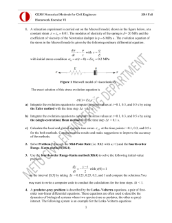


© Copyright 2026