1. finance

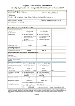
HONG KONG INSTITUTE FOR MONETARY RESEARCH
ANTI-COMPARATIVE ADVANTAGE: A PUZZLE IN
U.S.-CHINA BILATERAL TRADE
Jiandong Ju, Ziru Wei and Hong Ma
HKIMR Working Paper No.09/2015
April 2015
Hong Kong Institute for Monetary Research
香港金融研究中心
(a company incorporated with limited liability)
All rights reserved.
Reproduction for educational and non-commercial purposes is permitted provided that the source is acknowledged.
Anti-Comparative Advantage:
A Puzzle in U.S.-China Bilateral Trade*
Jiandong Ju
Shanghai University of Finance and Economics
Tsinghua University
Hong Kong Institute for Monetary Research
and
Ziru Wei
Tsinghua University
and
Hong Ma
Tsinghua University
April 2015
Abstract
From 1992 to 2011, the total trade volume between the U.S. and China increased by 25 times, and
China’s share in U.S. total imports increased from 5% to 20%. However, the U.S.’s share in China’s
total imports dropped from 11% to 8% in the same period. In the major categories of U.S. exports to
China, Waste & Scrap increased from 744 million dollars in 2000 to 7,562 million dollars in 2008, rising
916% times and becoming the No.1 product that the U.S exports to China. It is important to understand
what explains these structural changes, and to ask whether the principle of comparative advantage
determines the structure of U.S.-China bilateral trade. Interestingly, we find an “Anti-Comparative
Advantage” puzzle: the U.S. exports less to China in sectors where it has greater comparative
advantage, while China exports more to the U.S. in its sectors with greater comparative advantage. To
further study this issue, we extend Eaton-Kortum model of bilateral trade to multiple sectors and test it
empirically using US and China trade data. We find that after controlling for the importer’s demand,
trade costs and factor intensities, etc., comparative advantage cannot explain U.S.-China bilateral
trade flows. The puzzle survives various robustness checks.
JEL Classifications: F11, F14, F15
*
Ju: Tsinghua University and Shanghai University of Finance and Economics, Email: [email protected]; Wei:
Tsinghua
University,
Email:
[email protected];
Ma:
Tsinghua
University,
Email:
[email protected]. We thank China Center for International Economics Exchanges (CCIEE) for financial
support. We have benefited from discussions with Shang-Jin Wei and Justin Yifu Lin as well as participants of the
workshops and seminars at Beijing University, Nanjing University, Shanghai Jiaotong University and the 2012 Tsinghua
Winter Meeting in International Economics. However, we are responsible for all errors.
The views expressed in this paper are those of the authors, and do not necessarily reflect those of the Hong Kong Institute for
Monetary Research, its Council of Advisers, or the Board of Directors.
Hong Kong Institute for Monetary Research
1.
Working Paper No.09/2015
Introduction
From 1992 to 2011, total trade volume between the U.S. and China increased by 25 times, and
China’s share in U.S. total imports increased from 5% to 20%. By contrast, the U.S.’s share in China’s
total imports shrank from 11% in 1992 to 8% in 2011. In the same period, the U.S.’s trade deficit with
China increased by more than 150 times, from 1.45 billion USD to 235 billion. Figure 1 is from page
77 of the “2009 Report to Congress of the U.S.-China Economic and Security Review Commission”,
which reports major U.S.’s exports to China between 2000 and 2008.
1
While the U.S.’s share in China’s total imports declined, the total volume of U.S.’s exports to China
increased from 16,253 million USD in 2000 to 71,457 million USD in 2008, rising by 339%. Probably
most surprisingly, the top one product that the U.S. exports to China is Waste & Scrap, above
Semiconductors & Other Electronic Components, Oilseeds & Grains, and Aerospace Products &
Parts. Exports of Waste & Scrap from the U.S. to China increased from 744 million dollars in 2000 to
7,562 million dollars in 2008, rising by 916% times. Among them, Copper Waste and Scrap, and
Aluminum Waste and Scrap accounted for 5% and 4% of total U.S. exports to China in 2011,
respectively. U.S.’s exports to China as a share of total U.S. exports to the world in Copper Waste
and Scrap was only 8% in 1996, but increased to 69% in 2011.
2
This paper aims to understand what determines the structure of U.S.-China bilateral trade. In
particular, we want to investigate the role of comparative advantage. Our paper is related to the
recent empirical literature testing the Ricardian theory of comparative advantage. The Ricardian
model predicts that countries should produce and export relatively more in industries that are
relatively more productive. Costinot, Donaldson, and Komunjer (2012) and Costinot and Donaldson
(2012) apply the Eaton and Kortum model (2002) to multiple-country empirical tests and show that
Ricardo’s ideas are supported by the data. In this paper we extend Eaton-Kortum’s model to multiple
sectors in bilateral trade and empirically test the role of Ricardian comparative advantage in
determining the U.S.-China trade structure. In contrast to Costinot, Donaldson, and Komunjer (2012)
who derive a “difference-in-difference” form of an empirical equation based on the theory, we derive a
more straightforward “difference” form of the Ricardian test: the difference between the log of country
i’s exports to country n and the log of country n’s consumption of its own product is explained by the
log of relative productivities and relative unit costs between the two countries. Interestingly, we
observe a puzzling pattern in U.S.-China bilateral trade: we find that the U.S. exports less to China in
sectors where it has greater comparative advantage (measured by relative labor productivity or
relative TFP between U.S. and China). We call such an abnormal data pattern the “Anti-Comparative
Advantage Puzzle”. In contrast, the cross-sector pattern of China’s exports to the U.S. is consistent
with Ricardo’s idea. These results hold after controlling for demand size, trade costs and production
costs, and when we exclude metal products and processing trade. Regressions of multilateral trade
1
Readers are guided to the website: http://www.dtic.mil/dtic/tr/fulltext/u2/a520210.pdf
2
See Table 1 on page 5.
1
Hong Kong Institute for Monetary Research
Working Paper No.09/2015
flows further indicate that China is an outlier in the U.S.’s global exports.
An emerging literature has studied the pattern of China's export, and its influence on developed
3
countries, especially the U.S. China’s increasing globalization has not only brought a flood of cheap
products to consumers in advanced economies, but also raised concerns about the impact on global
4
imbalances (Krugman, 2010) and labor welfare (Autor, et al., 2012) . Most studies focus on China's
export, rather than other countries’ exports to China or their bilateral trade structure. One exception is
Hammer, Koopman, and Martinez (2009), which documents how exports of Advanced Technology
Products (ATP) from the U.S. to China have expanded rapidly in recent years, and become
increasingly concentrated in electronic products. This reveals the integration of both the U.S. and
China into the global supply chain of IT products. Our paper contributes to the literature with a
comprehensive examination of the bilateral trade structure between China and the US.
The anti-comparative advantage pattern in U.S. exports has been observed by other studies. Notably,
Berger et al. (2012) explored the declassified CIA documents to examine whether U.S. power was
used to influence countries’ trade decisions during the Cold War. Controlling for bilateral trade costs,
political ideology, and the supply of U.S. loans and grants, they found that CIA interventions have
increased imports of foreign countries from the U.S. Moreover, the increase concentrated in industries
where the U.S. had comparative disadvantage.
The rest of the paper is organized as follows. Section 2 provides an overview of U.S.-China trade
patterns and describes the “Anti-Comparative Advantage Puzzle”. Section 3 constructs a theoretical
model based on Eaton-Kortum (2002) for our estimation in later sections. Section 4 empirically tests
the role of comparative advantage in explaining U.S.-China bilateral trade. Section 5 provides
robustness checks. Section 6 concludes.
2.
Data
In this section, we describe the U.S.-China trade relationship focusing on structural changes in the
past 15 years by reviewing their top 10 trading industries in 2011. We then test the correlation
between the export structure of each and relative labor productivity, which reveals an anticomparative advantage pattern regarding U.S. exports to China. We compare exports in high-tech
sectors from the U.S. to China with those to India, to examine the possible effects from the demand
side.
3
Rodrik (2006) shows that China's export structure cannot be simply explained by its comparative advantage and free
market; the variety of the exported goods from China is much more complicated than what is suggested by its income
level, and moreover, this will be a key force for China’s future economic growth. Rodrik’s paper was followed up by further
studies, such as Schott (2008), Wang and Wei (2010), Amiti and Freund (2010).
4
Autor et al. (2013) show that increasing exposure to Chinese imports can account for a substantial portion of
unemployment in the US. It has also led to lower labor force participation and lower wages. Similarly effect on US job
losses is also documented in Berger and Martin (2011) with evidence at the industry level.
2
Hong Kong Institute for Monetary Research
2.1
Working Paper No.09/2015
Overview of U.S.-China Bilateral Trade Structures
Table 1 lists the top 10 industries measured by the value of the share of US exports to China in 2011,
at the 6-digit HS code level. For comparison, the export shares in 1996 are also shown. We focus on
manufacturing sectors. Here we define the export share of an industry in two ways: columns (1) and
1
(2) use Xshare , defined as the industry’s export value as a percentage of total US exports to China.
2
Columns (3) and (4) use Xshare , defined as the industry’s export value to China as a percentage of
5
1
total US exports to the world in the same industry. While Xshare has been commonly used to
2
measure trade structures, Xshare standardizes the export value of each industry by the exporter’s
overall competitive advantage to the world, which makes comparisons across industries more
6
sensible .
1
As Table 1 shows, according to Xshare , U.S. exports to China in 2011 were dominated by three
categories: capital intensive products (integrated circuits, vehicles), primary goods (cotton, woods),
and metal scraps (copper, aluminum and other ferrous wastes). The structure looked very different in
1996, when only cotton and air coolers were listed among the top exported products. The most
significant change came from combined metal wastes, the share of which grew from 1% to 11% in 15
2
years. Furthermore, when using Xshare , it shows that in most of the top 10 industries, China has
grown from a marginal buyer to a significant one, sometimes even the largest one. Again for listed
metal wastes, more than half of the US’s total exports are now sold to the Chinese market. This
indicates that U.S. export patterns to China have changed significantly, vis-a-vis the rest of the world.
Following the same definition in Table 1, Table 2 presents the top 10 industries by export value of
China’s exports to the U.S. in 2011. The industries are mostly labor-intensive products, such as toys
and footwear, and electronics products where China’s role in the global supply chain has increased.
2
As shown by Xshare , the U.S. is the main importer from China in these industries. Furthermore,
comparisons between 1996 and 2011 indicate that the pattern of China’s exports to the U.S. has
changed, but similar to the way in which its export patterns to the rest of the world has changed.
2.2
The Anti-Comparative Advantage Pattern
According to Ricardian theory, a country should export more in sectors where it has a comparative
advantage, and import more in sectors where it has comparative disadvantage. To test whether the
U.S.-China trade structure fits the Ricardian prediction, we follow Golub and Hsieh (2000) and adopt
5
Specifically,
XSharei1, c 
XSharei2，c 
6
Country c's export to its partner in sector i
(c=China, US) , and
Country c's total exports to its partner
Country c's export to its partner in sector i
(c=China, US)
Country c's total exports to the world in sector i
Otherwise if country c exports a low value of industry i to its partner, it may just reflect that country c is not a main
exporter in this industry, and it exports little to the rest of the world as well.
3
Hong Kong Institute for Monetary Research
Working Paper No.09/2015
relative labor productivity as a measure of comparative advantage. Labor productivity is defined as
value-added per worker. Based on the extended Eaton-Kortum model that we derive in the next
section, we expect a positive correlation between relative labor productivity and the export shares,
calculated as a country’s exports to its partner over the latter’s expenditure on home-produced goods
7
3
(output minus export) , labeled as Xshare . As a robustness check, we calculate the correlation
1
2
between relative labor productivity and Xshare and Xshare as defined above. The above variables
require data from the U.S. Census, UN COMTRADE, NBER-CES, and the Annual Industrial
Enterprise Survey of China’s National Bureau of Statistics. These databases have different industry
classifications and different time spans, which we harmonize into 240 manufacturing industries from
8
1998 to 2008. The time coverage allows us to utilize actual trade data and Chinese productivity data
9
for the whole period, while US productivity after the year 2006 is inferred from that of 2005 .
Table 3 summarizes the correlation coefficients between U.S.-China export shares and relative labor
3
productivity in the respective industries, with the last two columns based on Xshare , left and middle
1
2
two on Xshare and Xshare respectively. Since 2000, U.S. exports started to show an abnormal
pattern: under all three definitions, export shares became negatively correlated with relative
productivity, and the correlation coefficients have become increasingly negative in more recent years.
That is, the U.S. appears to export relatively smaller volumes to China in industries in which it has a
larger comparative advantage. The larger the comparative advantage is, the less the U.S. exports to
China, relative to the rest of the world. On the other hand, China’s exports to the U.S., as columns (2)
(4) and (6) show, present a pattern which is more consistent with the theory. Overall China’s export
patterns to the U.S. are consistent with the theory of comparative advantage.
2.3
China-India Comparison
The U.S. is widely regarded as having a comparative advantage in high-tech products compared to
developing countries. However, the anti-comparative advantage pattern in US exports to China could
be driven by the demand side. We lack sufficient information to examine the demand side effect fully.
A naïve and simple test is to compare the structure of US exports to China with its exports to a similar
developing country, India.
10
Table 4 lists the 15 most skill-intensive industries in the US and their skill intensity (as in column (1) ).
1
Columns (2) to (5) give the export shares to China and India respectively, where Xshare follows the
7
defined in equation (5) on page 7.
8
The industry classification is harmonized between 4-digit Standard Industrial Classification (SIC, 1987 version) and the
China’s 4-digit Industrial Classification.
9
NBER-CES database only provide data till the year of 2005. Therefore, we assume U.S. labor productivity didn’t change
since 2005, and use the value of 2005 as proxies for 2006 to 2008.
10
Here we use U.S. skill intensity to measure the technology content of each industry. The definition of skill intensity is
skilled labor income divided by total income. The data we use are also taken from the NBER-CES dataset. It adopts the
4-digit Standard Industry Classification (SIC), which provides more than 400 disaggregated industries.
4
Hong Kong Institute for Monetary Research
Working Paper No.09/2015
same definition as before, and Xshare
2
std
2
2
is the standardized Xshare , calculated as Xshare divided
by China’s (or India’s) share in U.S. total exports. Interestingly, export shares on both definitions are
almost always larger for India than for China.
From the simple descriptive statistics above, it seems that 1) the US exported less to China in those
products in which it had a comparative advantage, and 2) the US exported a greater share of those
products to India, though the two importers are of similar size. What drives such an anti-comparative
advantage pattern? In the following sections, we develop a theoretical model based on Eaton and
Kortum (2002). It takes into consideration demand size, trade costs, and production costs etc. at the
industry level. We then empirically test the importance of comparative advantage in determining U.S.China bilateral trade.
3.
11
The Model
This section extends the Eaton and Kortum (2002) model to multiple sectors. This setup leads to a
gravity equation investigating how sectoral bilateral trade is determined. Consumers in the two
countries have the same preference over the final goods, with utility given by:
𝑁
𝑈(𝑄1 , … , 𝑄𝑁 ) = ∏
𝑗=1
𝒂𝒋
𝑄𝑗
(1)
where 𝑄𝑗 is the quantity of the final good of sector 𝑗 (𝑗 = 1, … , 𝑁) and 𝑎𝑗 is the expenditure share of
good 𝑗 with 𝑎𝑗 ∈ (0,1), and ∑𝑁
𝑗=1 𝑎𝑗 = 1. Each sector j is composed of a continuum of varieties, indexed
by 𝜔𝑗 ∈ [0,1] and represented by:
𝑄𝑗𝑛
1
= (∫
0
(𝜎−1)/𝜎
𝑞𝑗𝑛 (𝜔𝑗 )
𝑑𝜔
𝜎/(𝜎−1)
𝑗)
(2)
where 𝑞𝑗𝑛 (𝜔𝑗 ) is the quantity of variety 𝜔𝑗 in sector 𝑗 consumed in country n. 𝜎 > 0 is the elasticity of
substitution.
Let 𝑐𝑗𝑖 be the unit production cost for the prospective exporter of product 𝑗 in country 𝑖. Country i’s
efficiency in producing variety 𝜔𝑗 of sector j is denoted as 𝑧𝑗𝑖 (𝜔𝑗 ) and follows the Frechet distribution:
𝐹𝑗𝑖 (𝑧) = 𝑒 −𝑇 𝑧
11
−𝜃
Exploring all possible explanation of this pattern is beyond the scope of this paper. Intuitively it might be driven by the
restricted supply from U.S., as well as sluggish demand from China in products that U.S. has comparative advantage.
However, above comparison between China and India implies that it’s more likely to be a supply side story. Most likely,
U.S. performed special export control policy towards China. See Section 5 for more details.
5
Hong Kong Institute for Monetary Research
Working Paper No.09/2015
where 𝑇𝑗𝑖 > 0 and 𝜃 > 1. The distribution is independent across sectors and countries. A larger 𝑇𝑗𝑖
implies better technology and a bigger 𝜃 implies less heterogeneity across varieties within the sector.
Let 𝑑𝑗𝑛𝑖 be the trade cost to deliver one unit of goods from country i to country n, 𝑑𝑗𝑛𝑖 > 1 for 𝑛 ≠
𝑖 and 𝑑𝑗𝑛𝑛 = 1. We assume that triangular inequality holds.
For a competitive market, we have country n’s import price of variety 𝜔 from country i:
𝑝𝑗𝑛𝑖 (𝜔) =
𝑐𝑗𝑖 𝑑𝑗𝑛𝑖
𝑧𝑗𝑖 (𝜔)
where the unit production cost𝑐𝑗𝑖 is given by a Cobb-Douglas aggregate index across different factors
f, namely, 𝑐𝑗𝑖 = ∏𝐹𝑓=0(𝑤𝑓𝑖 ) 𝑠 𝑓 .
Following the analysis by Eaton and Kortum (2002), exports from country i to country n in sector j are
given by:
𝑋𝑗𝑛𝑖 =
𝑇𝑗𝑖 (𝑐𝑗𝑖 𝑑𝑗𝑛𝑖 )−𝜃 𝑛
𝑇𝑗𝑖 (𝑐𝑗𝑖 𝑑𝑗𝑛𝑖 )−𝜃
𝑄𝑗 = 𝑁
𝑄𝑛
𝑛
∑𝑠=1 𝑇𝑗𝑠 (𝑐𝑗𝑠 𝑑𝑗𝑛𝑠 )−𝜃 𝑗
Φ𝑗
(3)
where 𝑄𝑗𝑛 is country n’s expenditure in sector j. Note that the sectoral output that country n produces
for her own market, which is a proxy for home-market demand, is:
𝑋𝑗𝑛𝑛 =
𝑇𝑗𝑛 (𝑐𝑗𝑛 )−𝜃
𝑠 𝑠 𝑛𝑠 −𝜃
∑𝑁
𝑠=1 𝑇𝑗 (𝑐𝑗 𝑑𝑗 )
𝑄𝑗𝑛
(4)
Using equations (3) and (4), we have:
−𝜃
𝑋𝑗𝑛𝑖 𝑇𝑗𝑖 (𝑐𝑗𝑖 𝑑𝑗𝑛𝑖 )
𝑇𝑗𝑖
𝑐𝑗𝑖 −θ 𝑛𝑖 −θ
=
=
(
)
∙
(
) ∙ 𝑑𝑗
−𝜃
𝑋𝑗𝑛𝑛
𝑇𝑗𝑛
𝑐𝑗𝑛
𝑇𝑗𝑛 (𝑐𝑗𝑛 )
(5)
Therefore, country n’s import value in sector j from country i, relative to its expenditure on home
production of sector j, depends on country i’s sectoral productivity relative to country n (i.e.,
country i’s relative production costs in producing j (i. e. ,
𝑐
𝑐
Tij
Tn
j
),
), and trade costs between the two countries
(𝑑𝑗𝑛𝑖 ). Taking logs, we obtain a gravity equation in equation (6), which we test empirically in the
following section:
6
Hong Kong Institute for Monetary Research
𝑙𝑛𝑋𝑗𝑛𝑖 = 𝑙𝑛𝑋𝑗𝑛𝑛 + 𝑙𝑛
4.
Working Paper No.09/2015
𝑇𝑗𝑖
𝑐𝑗𝑖
−
𝜃𝑙𝑛
− 𝜃𝑙𝑛𝑑𝑗𝑛𝑖
𝑇𝑗𝑛
𝑐𝑗𝑛
(6)
Empirical Results in Bilateral Trade
Based on equation (6), we propose the following econometric models for empirical analysis:
ln EX usj  0  1 ln HME cnj  2 ln RTechusj / cn  3 ln R( K / L)usj /cn  4 ln Tariff jcn   j
(7)
ln EX cnj  0  1 ln HME usj  2 ln RTechcnj /us  3 ln R( K / L)cnj /us  4 ln Tariff jus   j
(8)
The dependent variable 𝐸𝑋𝑗𝑢𝑠 is U.S.’s export to China of industry j, and 𝐸𝑋𝑗𝑐𝑛 indicates China’s
exports to the U.S. in the same industry. Both variables are obtained from the U.S. Census
Merchandise of Export/Import data. 𝐻𝑀𝐸𝑗𝑐𝑛 and 𝐻𝑀𝐸𝑗𝑢𝑠 is home market expenditure (output minus
export)
at
the
products.
𝑢𝑠/𝑐𝑛
𝑅𝑇𝑒𝑐ℎ𝑗
and
industry-level,
𝑐𝑛/𝑢𝑠
𝑅𝑇𝑒𝑐ℎ𝑗
representing
the
importer’s
demand
for
home
produced
define industry-level relative technology, with the numerator in the
superscript denoting the exporter and the denominator denoting the importer. In this and the following
sections, technology is mainly measured by labor productivity and TFP. In the multilateral regressions,
𝐾 𝑢𝑠/𝑐𝑛
and
𝐿
we use revealed comparative advantage to proxy for productivity. Similarly, 𝑅( )𝑗
𝐾 𝑐𝑛/𝑢𝑠
are
𝐿
𝑅( )𝑗
relative capital-labor ratios at the industry level, which reflect the relative factor prices given a CobbDouglas production function and therefore relative production costs across industries. Data for
productivity and the endowment variables are based on the U.S. NBER-CES dataset and China’s
Annual Survey of Industry Production. Finally, bilateral trade costs are measured by import tariff rates
at the industry level, denoted as 𝑇𝑎𝑟𝑖𝑓𝑓𝑗𝑐𝑛 and 𝑇𝑎𝑟𝑖𝑓𝑓𝑗𝑢𝑠 respectively. Tariff data are from the WITS
database. Note that the distance between both countries doesn’t change across industry so this is not
included as a variable in the bilateral regressions.
4.1
Benchmark Results
Using U.S.-China panel trade data for around 240 industries from 1998 to 2008, we use the
econometric specifications given by equations (7) and (8) to test for the “Anti-Comparative Advantage
Puzzle”. Regression outcomes are summarized in Table 5. The first three columns focus on the U.S.’s
exports to China, and the other three columns examine China’s export to the US. Columns (1) and (4)
give the benchmark results, following our theoretical model. Columns (2) and (5) include the
exporter’s industry level GDP to control for its production capacity, and year fixed effects to control for
aggregate shocks. Columns (3) and (6) add industry fixed effects to control for industry specific
shocks; however, there is a possibility that the industry fixed effect is too strong to rule out crossindustry differences in comparative advantage determining trade structure. Therefore we mainly rely
on results with only year fixed effects controls, namely columns (2) and (5). Across all specifications,
7
Hong Kong Institute for Monetary Research
Working Paper No.09/2015
the relative productivity coefficients for the first three columns are negative while those for the last
three columns are positive. This indicates that the more productive Chinese industries (relative to the
U.S.) export more to the U.S., while more productive American industries (relative to China) export
less to China. As expected, the effect of sectoral home-market expenditure and GDP are both positive
(or not significant). The US exports more in more capital intensive sectors according to column (1)
and (2). The negative sign of relative capital intensity in column (4) indicates that China exports more
to the US in its more labor intensive sectors, but in columns (5) and (6) it becomes less significant. As
expected, the sectoral exports become less if the tariff rate charged by the importing country is higher.
With the notable exception of the anti-comparative advantage patterns in US’s exports, the regression
results are consistent with the theory.
4.2
Robustness Checks
We add three robustness tests to further examine the “anti-comparative advantage puzzle” found in
the above.
4.2.1
Other Measurements of Technology
We first replace labor productivity with total factor productivity (TFP), measured via the Solow
Residuals. The industry level TFP is based on a three-factor Cobb-Douglas production function which
includes labor, capital and intermediary inputs. The labor and intermediary shares are estimated by
expenditure on these inputs divided by total output, and the capital share is derived as the residual.
Log TFP is therefore calculated as log real output minus the share of each input times their logged
value in real terms. Deflators for Chinese input and output are obtained from Brandt, Van Biesebroeck
and Zhang (2012), and US deflators come from the NBER-CES database.
Results are summarized in Table 6. The coefficients for relative TFP remain the same sign and are
significant as those in Table 5, except for column (2). Thus, the anti-comparative advantage puzzle
still holds.
4.2.2
Excluding Metal Products
As presented in Table 1, metal scraps accounted for 11% of U.S. exports to China in 2011. China is
the most important buyer for U.S. waste metals. One possible explanation is that as a mature postindustrial country, the United States has an abundant endowment in scrap metal, while a developing
country like China is relatively scarce in such resources. This is consistent with the Heckscher-Ohlin
factor endowment theory of international trade. Therefore, we drop all metal and metallic products
from U.S. exports to China, and redo the regressions with year fixed effects. Relative technology is
measured by both labor productivity and TFP. Results are reported in Columns (1) and (2) of Table 7.
It shows that almost all variables have the same sign and significance as in the benchmark results; in
particular, the anti-comparative advantage puzzle remains.
8
Hong Kong Institute for Monetary Research
4.2.3
Working Paper No.09/2015
Excluding Processing Trade
One prominent feature in U.S.-China bilateral trade is the prevalence of processing trade. It is
therefore natural to ask whether the pattern of U.S. exports to China could be distorted by those
products. So we further exclude processing exports in our regression. Due to data unavailability, we
restrict the panel data time coverage to 2000 to 2006. Results are reported in columns (3) and (4) of
Table 7. U.S./China relative technology, whether measured by labor productivity or TFP, has a
negative effect on U.S. non-processing exports to China as before.
5.
Empirical Results in Multilateral Trade
Is the anti-comparative advantage pattern specific to US-China trade, or a common phenomenon
affecting U.S. exports to other countries as well? To answer this question, we extend our empirical
model to a multiple country framework. Equation (7) is applied to all countries that import from the
U.S., with the importer’s home-market expenditure replaced by the importer’s sectoral GDP due to
data limitations. Export and tariff data are from the WITS database. The U.S. and the importing
countries’ GDP and capital intensity
12
at the industry level are taken from the United Nations Industrial
Development Organization (UNIDO) database. Chinese data are from the Annual Survey of Industrial
Enterprises. Note that in multilateral regressions, after controlling for industry level tariffs, there are
still other country-specific trade costs that affect U.S. exports to other countries (i.e., distance). We
use country dummies to further control these factors.
In terms of technology, due to limitations in data quality and availability, we adopt Balassa’s (1965)
definition of Revealed Comparative Advantage (RCA).
The RCA of country c in industry i is
calculated directly using international trade data according to Equation (9). 𝑅𝐶𝐴𝑐𝑖 >1 indicates country
c’s export share is larger than the world’s average export share in industry i, hence country c is
considered to have a comparative advantage in this industry relative to the rest of the world. The
relative technology can therefore be represented as exporter-to-importer’s relative RCA.
𝑅𝐶𝐴𝑗𝑐 =
𝑐𝑜𝑢𝑛𝑡𝑟𝑦 𝑐 ′ 𝑠 𝑒𝑥𝑝𝑜𝑟𝑡 𝑖𝑛 𝑖𝑛𝑑𝑢𝑠𝑡𝑟𝑦 𝑖 ⁄𝑐𝑜𝑢𝑛𝑡𝑟𝑦 𝑐 ′ 𝑠 𝑡𝑜𝑡𝑎𝑙 𝑒𝑥𝑝𝑜𝑟𝑡
𝑤𝑜𝑟𝑙𝑑 𝑒𝑥𝑝𝑜𝑟𝑡 𝑖𝑛 𝑖𝑛𝑑𝑢𝑠𝑡𝑟𝑦 𝑖 ⁄𝑤𝑜𝑟𝑙𝑑 𝑡𝑜𝑡𝑎𝑙 𝑒𝑥𝑝𝑜𝑟𝑡
(9)
To harmonize variables from different sources, we adopt the International Standard Industrial
Classification (ISIC) rev.3 for our multilateral analysis, which yields over 100 manufacturing industries
for each country. The UNIDO database has many missing values, and data quality varies widely by
country. We therefore filter our country sample by setting a minimum requirement of 70 industries with
all variables available, which leaves us with a sample of 37 importing partners for the U.S., including
China. See Table A1 in the appendix for a detailed country list.
12
Capital stock is not directly available in the UNIDO dataset. Instead, we use industry-year specific investment data which
was available in UNIDO, and apply a 15-year double declining balance method (Leamer, 1984, pages 230-234). The
initial year is 1970. Investment deflators are from the Penn World Table.
9
Hong Kong Institute for Monetary Research
Working Paper No.09/2015
We first run a full sample regression with both country and year fixed effects, as column (1) in Table 8
shows. Here the coefficients should again be interpreted as cross-industry differences. It shows that
the U.S./importer’s relative RCA has a positive sign, indicating that the U.S. exports more in industries
where it has a higher relative RCA, consistent with the theoretical model and standard trade theories.
All other variables have their expected sign as well.
A China dummy, which equals 1 when the importing country is China and zero otherwise, is interacted
with the U.S./importer’s relative RCA. We report the result in column (2), which includes country and
year fixed effects. Interestingly, the interaction term is negative and highly significant. This indicates
that US exports to China are significantly different from US exports to other countries in our sample,
which once again supports the anti-comparative advantage pattern that we documented earlier. The
above tests are repeated for India and Indonesia, as columns (3) and (4) of Table 8 show, revealing
that U.S.’s exports to India also show an abnormal pattern, but this is smaller in scale and less
significant, while U.S.’s exports to Indonesia are consistent with the comparative advantage theory.
6.
Discussions
A full investigation of the causes of the “Anti-Comparative Advantage Puzzle” in U.S.’s exports to
China is beyond the theme of this paper. Complaints have been made by China’s senior trade officials
on U.S. restrictions on high-tech exports. It has been reported that 2,400 categories of dual-use
commodities are banned for export to China by the US government (Chen, 2012).
13
There is a
growing body of evidence that U.S. restrictions on exports are outdated and may negatively affect US
companies’ export opportunities to China (AmCham China, 2009).
14
In Appendix B we provide a brief
review of U.S. export restrictions vis a vis China.
The ideal way to test whether US export controls may explain the anti-comparative advantage puzzle
that we have found in this paper is to construct an “US export control index”, to add it into the
regression for U.S. export to China as an additional control, and to see whether the coefficient on
comparative advantage becomes significantly and positive with the control variable. Unfortunately, we
15
lack sufficient information to build a continuous index consistent with our industry classifications . As
a compromise, we identify 34 control-related industries using a keyword match between the detailed
list of banned goods at a product level and our industry classification (see Table B2 in the Appendix).
This approach is limited by its inability to reflect the strength of US’s controls over each industry.
13
The claim was made by Mr. CHEN Deming, the former Minister of the Ministry of Commerce of China, in the 2012 China
Development Forum. See http://english.cntv.cn/program/newshour/20120319/114831.shtml
14
The report was jointly conducted by AmCham China and the American Chamber of Commerce in Shanghai. An abstract
of the research could be found online: http://www.amchamchina.org/article/5011
15
The most authorized information regarding US export control comes from The US Department of Commerce’s Bureau of
Industry and Security (http://www.bis.doc.gov/licensing/exportingbasics.htm). It lists 9 categories of dual-use products
required to go through special procedure to be sold abroad (see Table B1 in the Appendix for details). These categories
are too broad for our analysis, while the corresponding detailed product list follows unique classification method, which is
very difficult to be harmonized with our industry classification.
10
Hong Kong Institute for Monetary Research
Working Paper No.09/2015
However, comparing the US/China comparative advantage between control-related industries and the
others might shed some light on the cause of the puzzle.
As Table 9 shows, US/China relative labor productivity and relative TFP are both significantly higher
for control-related industries. This indicates that the intensity of U.S. export controls might be
positively correlated with US/China comparative advantage, and the previous regression coefficient
for US/China relative productivity may reveal a composite effect of both comparative advantage and
U.S. export controls. Specifically, in equation (6), the trade costs term 𝑑𝑗𝑛𝑖 could be decomposed into
the arithmetic product of two sub-terms, 𝑑𝑗𝑛𝑖∗ traditional trade costs, and 𝑐𝑜𝑛𝑡𝑟𝑜𝑙𝑗𝑛𝑖 as the US control
intensity, which is a function of 𝑇𝑗𝑖 /𝑇𝑗𝑛 . ubstituting the above into equation (6), we derive: S
𝑙𝑛𝑋𝑗𝑛𝑖 = 𝑙𝑛𝑋𝑗𝑛𝑛 + 𝑙𝑛
𝑇
𝑇
− 𝜃𝑙𝑛
𝑐
𝑐
𝑇
− 𝜃ln(𝑑𝑗𝑛𝑖∗ ∗ 𝑐𝑜𝑛𝑡𝑟𝑜𝑙𝑗𝑛𝑖 ( ))
𝑇
which implies:
𝑙𝑛𝑋𝑗𝑛𝑖 = 𝑙𝑛𝑋𝑗𝑛𝑛 + (𝑙𝑛
𝑇𝑗𝑖
𝑇𝑗𝑖
𝑐𝑗𝑖
𝑛𝑖
−
𝜃
ln
𝑐𝑜𝑛𝑡𝑟𝑜𝑙
(
))
−
𝜃𝑙𝑛
− 𝜃𝑙𝑛𝑑𝑗𝑛𝑖∗
𝑗
𝑇𝑗𝑛
𝑇𝑗𝑛
𝑐𝑗𝑛
(10)
The negative sign on the comparative advantage term (represented by the relative productivity) that
we found in the regression may be the composite effect of comparative advantage and export
controls. If we are able to properly take account of export controls, we should be able to see the “AntiComparative Advantage Puzzle” disappear or weakened.
7.
Conclusion
Since China’s WTO accession in 2001, the U.S.-China trade imbalance has grown, and has become
a major economic and political issue between the two countries. Instead of focusing on the exchange
rate, which seems to be a major concern for the trade imbalance, this paper explores the trade
structure between the two countries and provides a new insight to the trade imbalance between China
and the U.S..
We show that this is a puzzle in U.S.-China bilateral trade patterns. The U.S. exports less to China in
the sectors where it has greater comparative advantage; while China’s export to the U.S. fit the theory
of comparative advantage. Such a pattern is contrary to the prediction of standard comparative
advantage theory, thus we label it as an “Anti-Comparative Advantage Puzzle”. Intuitively, this puzzle
could be driven by U.S. restrictions on exports to China, or other common factors that affect bilateral
trade structures. However, comparing U.S. high-tech exports to China with India indicates China might
be treated differently, and mildly point towards a supply side story.
11
Hong Kong Institute for Monetary Research
Working Paper No.09/2015
On top of all these findings, we introduce a theoretical model which generates a bilateral trade
determination function at an industry level. It takes into consideration the size of demand, trade costs,
production costs, as well as comparative advantage. We use the model to empirically test the role of
comparative advantage in U.S.-China bilateral trade. Results show that U.S. exports to China follow
an Anti-Comparative Advantage pattern, a result that survives various robustness checks. Multilateral
regressions further indicate China has a very special position in the U.S.’s world export market, which
further rules out the possibility of a demand side story.
As pointed out in the AmCham China report, US companies have lost hundreds of millions in sales
due to real and perceived restrictions arising from US export controls. In almost all cases where sales
were lost, international non-US competitors provided equivalent products or services. Our findings
suggest the following policy implications. To solve the U.S.-China trade imbalance, increasing U.S.
exports to China could be mutually beneficial. In particular, increasing exports to China in sectors
where the U.S. has greater comparative advantages should be a good starting point.
12
Hong Kong Institute for Monetary Research
Working Paper No.09/2015
Reference
Amiti, M. and C. Freund (2010), “The Anatomy of China's Export Growth,” in R. C. Feenstra and S.-J.
Wei, eds., China's Growing Role in World Trade: 35-56.
Autor, D. H., D. Dorn and G. H. Hanson (forthcoming), “The China Syndrome: Local Labor Market
Effects of Import Competition in the United States,” American Economic Review, forthcoming.
Anderson, J. E. (1979), “A Theoretical Foundation for the Gravity Equation,” American Economic
Review, 69: 106–16.
Anderson, J. E. and E. van Wincoop (2003), “Gravity with Gravitas: A Solution to the Border Puzzle,”
American Economic Review, 93: 170–92.
Berger, B. and R. F. Martin (2011), “The Growth of Chinese Exports: An Examination of the Detailed
Trade Data,” Board of Governors of the Federal Reserve System International Finance
Discussion Papers.
Berger, D., W. Easterly, N. Nunn and S. Satyanath (forthcoming), “Commercial Imperialism? Political
Influence and Trade during the Cold War,” America Economic Review, forthcoming.
Bergstrand, J. H. (1989), “The Generalized Gravity Equation, Monopolistic Competition, and the
Factor-Proportions Theory in International Trade,” Review of Economics and Statistics, 71:
143–53.
Bergstrand, J. H. (1990), “The Heckscher-Ohlin-Samuelson Model, the Linder Hypothesis and the
Determinants of Bilateral Intra-Industry Trade,” Economic Journal, 100: 1216–29.
Brandt, L., J. Van Biesebroeck and Y. F. Zhang (2012), “Creative Accounting or Creative Destruction?
Firm-level Productivity Growth in Chinese Manufacturing,” Journal of Development Economics
97(2): 339-51.
Deardorff, A. V. (1998), “Determinants of Bilateral Trade: Does Gravity Work in a Neoclassical World?”
in J. A. Frankel, ed., The Regionalization of the World Economy, University of Chicago Press:
7–22.
Eaton, J. and S.S. Kortum (2002), “Technology, Geography, and Trade,” Econometrica, 70: 1741-79
Feenstra, R. (2004), The Advance International Trade: Theory and Evidence, Princeton University
Press.
13
Hong Kong Institute for Monetary Research
Working Paper No.09/2015
Feenstra, R. and G. Hanson (2004), “Intermediaries in Entrepôt Trade: Hong Kong Re-Exports of
Chinese Goods,” Journal of Economics & Management Strategy, 13(Spring): 3-35.
Feenstra, R., W. Hai, W. T. Woo and S.-L.Yao (1999), “The U.S.-China Bilateral Trade Balance: Its
Size and Determinants,” American Economic Review, May: 338-43.
Golub, S. S. and C.-T. Hsieh (2000), “Classical Ricaidian Theory of Comparative Advantage Revised,”
Review of International Economics, 8: 221-34.
Hammer, A., R. Koopman and A. Martinez (2009), “China’s Exports of Advanced Technology Products
to the United States,” Office of Economics Research Note, U.S. International Trade
Commission No.RN-2009-10F.
Hanson, G. H. and C. Xiang (2004), “The Home Market Effect and Bilateral Trade Patterns,” American
Economics Review, 94(4): 1108-29.
Helpman, E., M. Melitz and Y. Rubinesin (2008), “Estimating Trade Flows: Trading Patterns and
Trading Volumes,” Quarterly Journal of Economics, 123: 441-87.
Kamin, S., M. Marzzzi and J. Schindler (2006), “The Impact of Chinese Exports on Global Import
Prices,” Review of International Economics, 14: 179-201.
Krugman, P. (2010) “Killer Trade Deficits,” New York Times, 16 August 2010.
Leontief, W. (1953) “Domestic Production and Foreign Trade: The American Capital Position Reexamined,” Proceedings of the American Philosophical Society, 97: 332-49.
McKinnon, R. and G. Schnabl (2009), “China’s Financial Conundrum and Global Imbalances,” BIS
Working Papers No.277.
Wang, Z. and S.-J. Wei (2010), “What Accounts for the Rising Sophistication of China’s Exports?” in
R. C. Feenstra and S.-J. Wei, eds., China's Growing Role in World Trade, National Bureau of
Economic Research
Xu, Y.-P., G.-J.Lin and H.-Y. Sun (2010), “Accounting for the China-U.S. Trade Imbalance: An
Ownership-Based Approach,” Review of International Economics, 18: 540-51.
14
Hong Kong Institute for Monetary Research
Working Paper No.09/2015
Table 1. Top 10 Industries that U.S. Exported to China in 2011
Rank of
Industry (HS6)
% of U.S. total export to
1
2011
China (Xshare )
% of U.S. total export in
2
this industry (Xshare )
2011
1996
2011
1996
(1)
(2)
(3)
(4)
1
Copper waste and scrap
5%
0.5%
69%
8%
2
Electronic integrated circuits, monolithic
4%
0.4%
13%
1%
3
Vehicles, Spark-ignition Engine 1500~ 3000cc
4%
0.0%
13%
0.1%
4
Aluminum waste and scrap
4%
0.3%
72%
10%
5
Cotton (Not Carded or Combed)
4%
7.2%
30%
27%
6
Other Ferrous Waste and Scrap
2%
0.3%
17%
4%
7
Vehicles, Spark-ignition Engine>3000 cc
2%
0.0%
10%
0.0%
8
Air-coolers, Air Purifiers
2%
1.3%
14%
3%
9
Unbleached Kraft paper or paperboard
2%
0.2%
68%
10%
10
Tropical woods
1%
0.1%
54%
0.5%
Table 2. Top 10 Industries China Exported to the U.S. in 2011
Rank of
Industry (HS6)
2011
% of Chinatotal
% of China total export
export to U.S.
in this industry
1
2
(Xshare )
1
Portable digital automatic data processing
(Xshare )
2011
1996
2011
1996
(1)
(2)
(3)
(4)
11%
0.1%
33%
44%
3%
0.1%
16%
7%
machines (ADP), weight<10 kg
2
Transmission Apparatus Incorporating
Reception Apparatus
3
Reception Apparatus For Color Television
2%
0.1%
33%
4%
4
Parts and Accessories of the ADP Machines
2%
2.2%
18%
34%
5
Storage units
2%
1.3%
33%
30%
6
Other apparatus
2%
0.0%
19%
14%
7
Other printing machinery
2%
0.0%
28%
5%
8
Other Toys
1%
3.1%
36%
47%
9
Other Footwear With Uppers of Leather
1%
5.2%
50%
69%
10
Input or output units for ADP machines
1%
1.8%
28%
23%
Source: World bank WITS database (UN Comtrade)
15
Hong Kong Institute for Monetary Research
Working Paper No.09/2015
Table 3. Correlation between Export Shares and Exporter-to-Importer’s Relative Productivity,
1998-2008
1
Corr (Xshare , relative
year
2
Corr (Xshare , relative productivity)
3
Corr (Xshare , relative productivity)
productivity)
(1) U.S. to CN
(2) CN to U.S.
(3) U.S. to CN
(4) CN to U.S.
(5) U.S. to CN
(6) CN to U.S.
1998
0.043
0.203
0.024
0.235
0.086
0.238
1999
0.025
0.139
0.000
0.116
0.062
0.188
2000
-0.027
0.074
-0.060
0.101
-0.014
0.135
2001
-0.060
0.191
-0.076
0.135
-0.055
0.231
2002
-0.026
0.075
-0.025
0.127
-0.006
0.172
2003
-0.117
0.038
-0.148
0.091
-0.112
0.160
2004
-0.129
0.101
-0.136
0.162
-0.083
0.188
2005
-0.123
0.054
-0.115
0.115
-0.066
0.122
2006
-0.107
-0.037
-0.135
-0.044
-0.064
0.034
2007
-0.081
-0.035
-0.150
0.078
-0.072
0.084
2008
-0.106
-0.087
-0.175
-0.032
-0.046
0.002
Source: Author’s calculation.
Table 4. U.S. High-Tech Exports to China and India, SIC4, 2005
SIC code
Products
Skill-intensity of U.S.
XShare
1
Xshare
2
std
China
India
China
India
3769
Space vehicle equipment
0.808
0.0%
0.0%
0.01
0.13
3826
Analytical instruments
0.801
1.3%
1.6%
1.62
2.03
3825
Instruments to measure electricity
0.794
1.4%
1.7%
1.52
1.79
3577
Computer peripheral equipment
0.787
0.9%
1.8%
0.80
1.68
3578
Calculating, accounting equipment
0.783
0.1%
0.1%
1.30
1.27
3812
Search and navigation equipment
0.772
0.4%
1.0%
0.66
1.74
3661
Telephone and telegraph apparatus
0.756
1.7%
3.1%
1.41
2.50
3844
X-ray apparatus and tubes
0.754
0.6%
1.0%
1.46
2.53
3663
Radio, communications equipment
0.748
0.4%
2.4%
0.47
2.82
3571
Electronic computers
0.741
3.2%
3.7%
1.13
1.30
2835
Diagnostic substances
0.731
0.2%
0.6%
0.38
1.02
3579
Office machines
0.726
0.1%
0.1%
1.00
0.84
3572
Computer storage devices
0.707
0.2%
0.8%
0.49
2.49
3669
Communications equipment
0.705
0.1%
0.2%
1.01
1.96
3489
Ordnance and accessories
0.704
0.0%
0.0%
0.01
0.05
16
Hong Kong Institute for Monetary Research
Working Paper No.09/2015
Table 5. Benchmark Regressions for U.S.-China Bilateral Trade, 1998 to 2008
Dependent variables: Log U.S. export to China in column (1) to (3), and Log China export to the U.S.
in column (4) to (6)
U.S. export to China
VARIABLES (in log terms)
China export to the U.S.
(1)
(2)
(3)
(4)
(5)
(6)
Importer’s consumption of its
0.480***
0.138***
0.159***
0.460***
0.174***
0.149**
own production by industry
(0.0302)
(0.037)
(0.040)
(0.057)
(0.053)
(0.060)
0.607***
0.375***
0.072*
0.064
(0.067)
(0.101)
(0.040)
(0.042)
Exporter’s GDP by industry
Relative labor productivity,
-0.428***
-0.255***
-0.130*
1.569***
0.182**
0.139*
Exporter/Importer
(0.0545)
(0.070)
(0.075)
(0.037)
(0.071)
(0.072)
Relative K-intensity,
0.293***
0.208***
0.043
-1.050***
0.096
0.141*
Exporter/Importer
(0.0654)
(0.079)
(0.088)
(0.068)
(0.079)
(0.082)
Tariff charged by importer
-0.158***
-0.090**
-0.042
-0.097***
-0.057***
-0.058***
(0.0347)
(0.035)
(0.036)
(0.021)
(0.019)
(0.019)
9.533***
9.405***
10.431***
14.067***
13.308***
13.788***
(0.618)
(0.728)
(0.922)
(0.857)
(0.950)
(1.067)
2,433
2,433
2,433
2,370
2,370
2,370
Industry FE
NO
NO
YES
NO
NO
YES
Year FE
NO
YES
YES
NO
YES
YES
Constant
Observations
17
Hong Kong Institute for Monetary Research
Working Paper No.09/2015
Table 6. Robustness Check: Technology Measured by Relative TFP, 240 Industries, 1998 to
2008
Dependent variables: Log U.S. export to China in column (1) and (2), and Log China export to the U.S.
in column (3) and (4)
U.S. export to China
VARIABLES (all in log terms)
China export to the U.S.
(1)
(2)
(3)
(4)
0.520***
0.177***
0.146***
0.147***
(0.027)
(0.036)
(0.055)
(0.051)
0.494***
0.479***
0.674***
0.089**
(0.066)
(0.064)
(0.026)
(0.038)
-0.625***
0.074
1.079***
0.451***
(0.097)
(0.119)
(0.100)
(0.120)
0.086
0.043
0.092
0.294***
(0.067)
(0.067)
(0.071)
(0.069)
-0.197***
-0.092**
-0.073***
-0.055***
(0.035)
(0.036)
(0.021)
(0.019)
4.242***
9.141***
5.066***
12.983***
(0.642)
(0.727)
(0.922)
(0.946)
2,422
2,422
2,347
2,347
Industry FE
NO
NO
NO
NO
Year FE
NO
YES
NO
YES
Importer’s consumption of its own production by industry
Exporter’s GDP by industry
Relative TFP, Exporter/Importer
Relative K-intensity, Exporter/Importer
Tariff charged by importer
Constant
Observations
18
Hong Kong Institute for Monetary Research
Working Paper No.09/2015
Table 7. Robustness Check: Excluding Metal Products and Processing Trade, 240 Industries,
1998 to 2008
Dependent variable: Log U.S. export to China at industry level
No metal products: 1998-2008
VARIABLES (all in log terms)
China’s consumption of its own production by industry
U.S. GDP by industry
Relative labor productivity, U.S./China
(1)
(2)
(3)
(4)
0.143***
0.179***
0.0979**
0.150***
(0.0370)
(0.0356)
(0.0460)
(0.0436)
0.596***
0.504***
0.620***
0.528***
(0.0682)
(0.0640)
(0.0807)
(0.0782)
-0.254***
-0.303***
(0.0693)
(0.0875)
Relative TFP, U.S./China
Relative K-intensity, U.S./China
No processing trade: 2000-2006
-0.117
-0.160
(0.0982)
(0.173)
0.204***
0.0242
0.365***
0.169*
(0.0785)
(0.0648)
(0.103)
(0.0905)
-0.0957***
-0.0955***
-0.0635
-0.0589
(0.0350)
(0.0350)
(0.0615)
(0.0618)
9.433***
8.961***
10.69***
10.06***
(0.733)
(0.729)
(0.930)
(0.947)
2,360
2,360
1,556
1,556
Number of industry
218
218
225
225
Year Fixed effect
YES
YES
YES
YES
Tariff charged by China
Constant
Observations
19
Hong Kong Institute for Monetary Research
Working Paper No.09/2015
Table 8. Robustness Check: Multi-Lateral Regressions, 4-Digit ISIC, 1998 to 2008
Dependent variable: Log U.S. export to 37 countries at industry level
VARIABLES (all in log terms)
Importer's GDP by industry
U.S. GDP by industry
Relative RCA, U.S./importer
(1)
(2)
(3)
(4)
0.099***
0.093***
0.099***
0.101***
(0.016)
(0.016)
(0.016)
(0.016)
0.672***
0.680***
0.673***
0.669***
(0.028)
(0.028)
(0.028)
(0.028)
0.087***
0.103***
0.091***
0.080***
(0.011)
(0.012)
(0.012)
(0.012)
China*Relative RCA
-0.212***
(0.040)
India*Relative RCA
-0.112*
(0.060)
Indonesia*Relative RCA
0.220***
(0.060)
Relative k-intensity, U.S./Importer
0.047**
0.042**
0.046**
0.044**
(0.020)
(0.020)
(0.020)
(0.020)
-0.181***
-0.175***
-0.182***
-0.181***
(0.014)
(0.014)
(0.014)
(0.014)
-6.881***
-6.951***
-6.908***
-6.866***
(0.649)
(0.649)
(0.649)
(0.650)
Observations
9,539
9,539
9,539
9,539
Country FE
YES
YES
YES
YES
Year FE
YES
YES
YES
YES
Tariff charged by importer
Constant
20
Hong Kong Institute for Monetary Research
Working Paper No.09/2015
Table 9. US-to-China Comparative Advantage Comparison and T-test Results
Productivity
measurement
Control-related
Control-irrelevant
T-test (H0: US/China
industries
industries
comparative advantage is
Mean (std dev)
Mean (std dev)
higher for control-related
industries)
Labor productivity
0.94 (0.04)
0.79 (0.01)
Not reject at 1%
TFP
0.20 (0.03)
0.12 (0.01)
Not reject at 1%
21
Hong Kong Institute for Monetary Research
Working Paper No.09/2015
Figure 1. Major U.S. Exports to China, 2000-2008 (in millions of U.S. $)
22
Hong Kong Institute for Monetary Research
Working Paper No.09/2015
Appendix A. Additional Tables and Figures
Table A1. List of Countries Used in the Multilateral Regression
No.
ISO3
Country
No.
ISO3
Country
1
AU.S.
Australia
20
LKA
Sri Lanka
2
AZE
Azerbaijan
21
LTU
Lithuania
3
BGR
Bulgaria
22
LVA
Latvia
4
BOL
Bolivia
23
MAR
Morocco
5
CHL
Chile
24
MEX
Mexico
6
CHN
China
25
MLT
Malta
7
COL
Colombia
26
MWI
Malawi
8
CYP
Cyprus
27
MYS
Malaysia
9
CZE
Czech Republic
28
NOR
Norway
10
ECU
Ecuador
29
NPL
Nepal
11
ETH
Ethiopia(excludes Eritrea)
30
OMN
Oman
12
GEO
Georgia
31
POL
Poland
13
HUN
Hungary
32
SGP
Singapore
14
IDN
Indonesia
33
SVK
Slovak Republic
15
IND
India
34
SVN
Slovenia
16
IRN
Iran, Islamic Rep.
35
SWE
Sweden
17
JOR
Jordan
36
TUR
Turkey
18
JPN
Japan
37
URY
Uruguay
19
KOR
Korea, Rep.
23
Hong Kong Institute for Monetary Research
Working Paper No.09/2015
Appendix B. The History of U.S. Export Control
The U.S. has a long history of export restrictions towards China, which can be dated back to the Cold
War. In 1948, the U.S. proposed to establish Committee Controlling East-West Trade (COCOM) in
order to implement military embargo against the socialist countries. Then in 1952, by the impact of the
Korean War, COCOM set up the “China Commission”, implementing stricter embargo policies on
China than the Soviet Union and Eastern European; the ban list for China included 500 more items
than the international ban list. Eventually, with China's economic development and the progress of
U.S.-China diplomatic relation, the strength of U.S. export control towards China had been weakened
gradually. However in 1989 the United States again suspended its cooperation with China on militarytechnical projects, and all other COCOM members announced the termination of their previous relax
on high-tech exports to China. In 1995, the U.S. developed an export priority system based on the
exporting products and their technology content, dividing countries in the world into 8 categories.
China was drawn in the sixth category “Outsiders” together with India and Singapore, which is below
the category of “Comrades” where Russia, Ukraine, Bulgaria and Romania belonged to, and over
“The States of Concern” with members like Iraq, Iran, North Korea and Libya etc.
In 1996, the United States and other 32 western countries signed the "Wassenaar Agreement” (WA),
deciding to implement the new control list and information exchange rules since November 1, 1996;
China was still one of the banned countries. WA included two control lists: one is a list of dual-use
goods and technologies; the other is the military list.
The most recent adjustment of U.S. export control policy occurred on June 19, 2007, when the
Bureau of Industry Security in the U.S. Department of Commerce officially announced the “Revisions
and Clarification of Export and Re-export Controls for the People’s Republic of China (PRC); New
Authorization Validated End-User; Revision of Import Certificate and PRC End-User Statement
16
Requirements” . This policy prohibited the exporting of 9 categories of products (See Table B1 below)
to China, all of which are classified as with technologies likely to “enhance China's military strength”.
Besides, the U.S. “Validated End-User” plan regulates that only “Trusted clients” can import restricted
goods without special authorization. By the end of 2009, only five companies in China had received
such VEU status, but none of which is local owned enterprise.
16
“Revisions and Clarification of Export and Re-export Controls for the People’s Republic of China (PRC); New
Authorization Validated End-User; Revision of Import Certificate and PRC End-User Statement Requirements”, Federal
Register, 72(117), Tuesday, June19, 2007, Rules and Regulations, Department Of Commerce Bureau of Industry and
Security.
24
Hong Kong Institute for Monetary Research
Working Paper No.09/2015
Table B1. Product Categories of U.S. Export Control
Category
Description
0
Nuclear Materials, Facilities & Equipment (and Miscellaneous Items)
1
Materials, Chemicals, Microorganisms, and Toxins
2
Electronics
3
Computers
4
Telecommunications
5
Information Security
6
Sensors and Lasers
7
Navigation and Avionics
8
Marine
9
Propulsion Systems, Space Vehicles and Related Equipment
25
Hong Kong Institute for Monetary Research
Working Paper No.09/2015
Table B2. U.S. Export Control Related Industries
Product Category
SIC and CIC harmonized Industry
0
Nuclear fuel
0, 2
Arms and Ammunition
0, 1, 2, 9
Pumping equipment
0, 8
Air compressors
1
Alkalies and chlorine gases
1
Nitrogenous fertilizers
1
Explosives
1
Carbon and graphite
1
Refractory ceramics
1
Smelting and refining of nonferrous metals
1
Medicinal chemicals and botanical products
1
Flat glass
1
Biological products
1, 2
Steel rolling process
1, 3
X-ray apparatus etc.
2
Carburetors and valves
2
Machine tools, metal cutting types
2
Machine tools, metal forming types
2
Welding and soldering equipment
2
Ball and roller bearings
3
Switchgear and switchboard apparatus
3
Electronic capacitors
3
Semiconductors
3
Electron tubes
4
Electronic components
4
Electronic computers
6
Optical instruments and lenses
6, 7
Search, detection, navigation etc.
8
Boiler
8
Photographic equipment and supplies
9
Internal combustion engines
9
Aircraft and parts
9
Guided missiles and space vehicles
9
Motors and generators
26