1. science
2. ecology
3. pollution

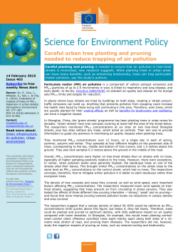
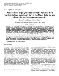
Aerosol and Air Quality Research, 15: 556–571, 2015
Copyright © Taiwan Association for Aerosol Research
ISSN: 1680-8584 print / 2071-1409 online
doi: 10.4209/aaqr.2014.04.0075
Monitoring, Source Identification and Health Risks of Air Toxics in Albuquerque,
New Mexico, U.S.A.
Ilias G. Kavouras1,2*, David W. DuBois1,3, George Nikolich1, Vic Etyemezian1
1
Division of Atmospheric Sciences, Desert Research Institute, Las Vegas, Nevada, USA
Department of Environmental and Occupational Health, Fay W. Boozman College of Public Health, University of
Arkansas for Medical Sciences, Little Rock, Arkansas, USA
3
Department of Plant and Environmental Sciences, New Mexico State University, Las Cruces, New Mexico, USA
2
ABSTRACT
Air toxics were monitored in three locations in Albuquerque, New Mexico, U.S.A representing different land use
configurations to determine the air toxics concentration gradient and factors controlling their ambient levels and to assess
potential health impacts. The total polycyclic aromatic hydrocarbons (PAHs), heavy metals and volatile organic
compounds (VOCs) concentrations at all sites ranged from 18.0 to 323.8 ng/m3, from 5.7 to 122.0 ng/m3 and from 0.1 to
18.7 ppbv, respectively. Sources of air toxics were determined using coupled positive matrix factorization and linear
regression analysis. For PAHs, a mixture of emissions from traffic, oil residues and wood burning was identified. The
comparison of PAHs relative distributions in Albuquerque to those emitted from three types of woodstoves showed a good
correlation with emissions from non-catalytic woodstoves. The values for toluene/benzene, xylene/benzene and
xylene/toluene ratios in Albuquerque indicated that traffic was the major source of aromatic VOCs. In addition, regression
analysis of air toxics to daily PM2.5 source contributions showed that the vast majority of aromatic VOCs and PAHs were
strongly associated with the secondary NO3– source category, providing additional evidence of the significant role of
traffic emissions of air toxics and PM2.5 in Albuquerque. A small fraction of PAHs and heavy metals was associated with
road dust, indicating that mechanically released dust particles may be contaminated by oil residues and vehicle exhausts.
The annual hazard quotient values for benzene, toluene, xylene and methylene chloride were typical for urban communities
dominated by traffic emissions and similar to those estimated for other urban areas in the U.S. The annualized cancer risks
for benzene and methylene chloride were lower than 1-in-a-million.
Keywords: Air toxics; Hazardous air pollutants; Health effects/risks; PAHs; Toxic air pollutants; Toxic metals; Urban aerosols.
INTRODUCTION
There are 188 hazardous air pollutants (HAPs), or air
toxics, that require specific attention, long-term monitoring,
health risk assessment and, eventually, regulation under the
Clean Air Act and its Amendments (CAAA), because they
have been associated with a wide variety of adverse health
effects, including cancer, neurological effects, reproductive
and developmental effects (Delfino, 2002; Leikauf, 2002;
Windham et al., 2006). These air toxics are emitted from
multiple sources, including major stationary, area and mobile
sources (Ozkaynak et al., 2008; Logue et al., 2009). The
implementation of CAAA led to the development of the
Integrated Urban Air Toxics Strategy (IUATS) and the
*
Corresponding author.
Tel.: +1-501-526-6627; Fax: +1-501-526-6750
E-mail address: [email protected]
Air Toxics Program (ATP) which included the detailed
investigation of a subset of 33 HAPs including aromatic
hydrocarbons (e.g., benzene and its derivatives), halocarbons,
heavy metals (e.g., As, Hg, Ni), polycyclic aromatic
hydrocarbons (PAHs) and diesel particles in urban areas
(USEPA, 2000; Kyle et al., 2001). In addition, the National
Air Toxics Assessment (NATA) program has been developed
to monitor ambient concentrations, evaluate the impact of
sources nationwide and assess the health risks.
The Albuquerque, New Mexico (NM), U.S.A. greater
metropolitan area has almost 800,000 residents (Fig. 1). It
is located by the Rio Grande River and the intersection of
Interstate-40 and Interstate-25 highways. Urban growth and
recent improvements in the transportation network have
contributed to Albuquerque’s development of industry. The
major activities include manufacturing (electronic equipment,
semiconductors, missile guidance systems, surgical
appliances, transportation equipment and parts), printing
and publishing and food processing. Major regional point
sources are two gas-fired power plants and a coal fired
Kavouras et al., Aerosol and Air Quality Research, 15: 556–571, 2015
557
Fig. 1. The study region, land use and the locations of air toxics monitoring sites in Albuquerque, NM. (Monitoring sites:
R: Reference, S1 and S2: Satellites sites 1 and 2).
cement plant. The coal-fired Four Corners Power Plant is
one of the largest fossil-fuel steam-driven power plants in
the world. There is also a power plant to the west, between
Grants and Gallup, New Mexico and oil refineries located
outside of Albuquerque. Most of these activities are controlled
through the Maximum Achievable Control Technology
standards. The 2002 NATA analysis showed that the lifetime
cumulative cancer risk (30 in a million), neurological hazard
index (4.6 × 10–2) and respiratory hazard index (3.1) in
Bernalillo County, New Mexico were among the highest
estimated in the US (higher than the 75th percentile among
all counties (USEPA, 2002a). The Pilot City Monitoring
Program (PCMP) in 2001–2002 showed that the cancer
risk and toxicity due to inhalation, calculated using EPA’s
Prioritized Chronic Dose-Response values for screening risk
assessments to the local population in the greater Albuquerque
area was up to 12.44 in a million for benzene, especially
for those residing in the vicinity of industrial/commercial/
warehousing activities (USEPA, 2002b).
We carried out a community-scale monitoring program
in order to characterize air toxics concentrations and assess
their effects on living standards and human health in and
around the city of Albuquerque, NM. The objectives of
this study were: (i) measure ambient concentration levels
of air toxics within specific community regions in the city
of Albuquerque; (ii) identify and evaluate the impact of air
toxics sources; and (iii) assess adverse health impacts from
exposure using risk assessment models.
Kavouras et al., Aerosol and Air Quality Research, 15: 556–571, 2015
558
MATERIALS AND METHODS
Sampling
A map of the Albuquerque area, showing major interstate
highways, land use and the local air quality monitoring
sites is presented in Fig. 1. The reference site (R) was
located at the existing 2ZM site (Del Norte High School;
Air Quality System (AQS) ID: 350010023), northeast of
the intersection of I-25 and I-40. O3, PM10, PM2.5 CO, NOx
and meteorological parameters were monitored at this site
by AQD. In addition, this site has been used in a previous
pilot-scale air toxics study (USEPA, 2002b). A major source
at this site is the high density traffic from the nearby
intersection of San Mateo and Montgomery. There were
also a number of area sources such as filling stations, dry
cleaners and automotive repair shops. The satellite sites
included: (i) S1: 2ZH (North Valley; AQS ID: 350011013)
located northwest of the reference site in the North Valley
community. One of the major sources in the area is the Intel
computer chip manufacturing plant which was about 3.2
km to the northwest. Other area sources included filling
stations and emissions from sand and gravel plants to the
southeast. O3, CO and PM10 and PM2.5 were measured at
2ZH; and (ii) S2: 2ZV (South Valley, AQS ID: 350010029)
was located south-southwest of the reference site in the
South Valley community, which represented a diversity in
land use characterized by a mix of urban and rural
population densities as well as industrial and commercial
expansion. Urban growth began spreading into the South
Valley from the north and along its major streets. Industrial
activities included a power station, the City sewage treatment
plant, asphalt plants and tanks farms, auto dismantlers, brick
manufacturing, a chicken farm, and a meat packing plant.
O3, PM10, and meteorological parameters were monitored
continuously at 2ZV, which has been used in prior pilotscale air toxics studies (USEPA, 2002b).
The schedule and frequency of sampling of volatile organic
compounds (VOCs), polycyclic aromatic hydrocarbons
(PAHs) and heavy metals is presented in Table 1. 24-hr
integrated VOCs were measured using the Method TO-15 by
the New Mexico State Laboratory Division (SLD) (USEPA,
1999a). Ambient samples were collected using CS1200
samplers equipped with TM1000 Start/stop timers and 6-L
SUMMA canisters and analyzed, using a preconcentrator
(Model 7100, Entech Instruments Inc, USA) and a gas
chromatography (Carlo Erba GC-8060, CE Elantech Inc,
USA) equipped with a mass spectrometer (Model MD-800,
Fisons, Inc. United Kingdom). In addition, two intensive
monitoring periods (IMP) during which hourly measurements
of VOCs at the reference site were measured in February
and June 2008, using a SRI gas chromatography system
(Model TO-14, SRI Instruments, USA). A multi-component
certified calibration standard was obtained (Item No.
0102AZ00004ZCL, Scott Specialty Gases, USA). PAHs
and heavy metals were measured at the reference and
satellite sites on a 1-in-6 day frequency. Samples were
collected by Environmental Health Department of the City
of Albuquerque staff and analyzed by ERG Inc. using the
TO-13A and ERG standard protocols (US EPA, 1999b;
ERG, 2005). A portion of the quartz filters (1-cm2) was
also analyzed for elemental and organic carbon content
(EC/OC) at Desert Research Institute’s Environmental
Analysis Facility (Chow et al., 2001).
Source Apportionment
The Positive Matrix factorization (PMF) receptor model
was used to identify the major sources of PM2.5 in the
study area and to estimate the contributions of major sources
and source types to the PM2.5 mass. The concentrations of
PM2.5 mass and chemical species measured at the NCore
site in Albuquerque (reference site in our study) for the
study period were retrieved from US EPA’s AQS. Sampling
was done in 1 every 3 days frequency using a four channel
speciation sampler. Elements (from Na to U) were measured
by spectroscopy (X-ray fluorescence, PIXE, ICP, ICP-MS);
water-soluble ions (sulfate, nitrate, chloride, ammonium,
sodium, potassium, calcium and magnesium) by ion
chromatography and colorimetry; and elemental and organic
carbon (EC and OC, respectively) by thermal optical
reflectance method. PMF is a least squares formulation of
factor analysis with built-in non-negativity constraints
(Paatero and Tapper, 1994; Paatero, 1997). Through a
solution that minimizes the objective function (Q in Eq. (1))
based on measurements uncertainties.
 x  n  g xf  
 k 1 ik kj 
ik
Q   
 ij

i k 1 


n
m
(1)
where xik and σik are the concentration and associated
uncertainty of k-species in i-sample, gik is the contribution
of the j-factor to particle mass in i-sample and fkj is the
mass fraction of j-species on k-factor, the source contribution
(G(nxp)) and the source profile matrices (F(pxm)) where p is
the number of sources are computed from the concentrations
of m-aerosol species for n-sampling days (X(nxm)). The
optimum number of factors (sources) and the Fpeak value (that
defines the rotation) were selected on trial and error
analysis of the solutions using a set of statistical tools and
by comparison of the source profiles with previous source
Table 1. Sampling period and frequencies of air toxics in Albuquerque, New Mexico.
Compounds
VOCs (24-hr canister)
VOCs (1-hr online GC)
PAHs
Heavy metals
Period
September 2007–August 2008
and December 2008–March 2009
February and June 2008
December 2008–March 2009
December 2008–March 2009
Location and frequency
Reference and satellite sites; 1-in 6 days
Reference site; Every hour
Reference and satellite sites; 1-in 6 days
Reference and satellite sites; 1-in 6 days
Kavouras et al., Aerosol and Air Quality Research, 15: 556–571, 2015
profiles (Paatero et al., 2002, 2005). Missing concentration
data are replaced by the geometric mean of the measured
concentrations while missing uncertainties are substituted
by four times the geometric mean of measured uncertainties.
In this effort, we run the PMF model in the robust method
with α = 4.0 using the error model “–12” (that uses observed
values). We also added an additional modeling uncertainty
of 25% to reduce modeling errors. We initially ran the
model for 3 to 20 factors. The configuration includes 20 runs
with random seed per each run. All base run results were
converged which implied that the model had found the
local minima. For more than 6 factors, the Q value did not
change significantly, indicating that most of the variation
was explained by five to six factors. The solutions for that six
or more factors were rejected because they had excessive
rotational freedom. The four-factor model was rejected
because two factors, namely biomass burning and traffic
emissions, were merged into a single factor. For the fivefactor model, more than 90% of the residuals for individual
chemical species were normally distributed between –3
and +3, indicating good agreements of the fit to the
observed values. The bootstrap configuration included 200
runs, minimum r value of 0.75 and suggested block of 6 with
a random seeding. The interquartile ranges for individual
compounds were ± 20%.
Five-factor models with Fpeak values lower than –1.5 or
higher than 1.5 did not converge into a solution. Finally, a
five factor model with a rotation with Fpeak = –0.5 was
selected based on the profiles of sources and the agreement
between the calculated and estimated mass and elementals
concentrations. The contributions of the retained factors to
the individual PM2.5 components were computed using a
least-squares multivariate linear regression model (Song et
al., 2001)
p
X ik  a    f k   k  gik 
(2)
k 1
where βk is the regression coefficient or scaling constant to
convert the factor profiles and contributions to μg of
compounds/μg of PM2.5 and μg/m3, respectively. The
intercept, α, was attributed to other PM2.5 sources. Negative
regression coefficients indicated that there were too many
factors. The coefficient of variation of the root mean square
error, CV(RMSE) was used to evaluate the residuals between
measured and predicted PM2.5 and individual chemical
species values. It was defined as the RMSE normalized to
the mean of the observed values
CV  RMSE  
RMSE
X measured
 X
n

i 1
predicted , i
 X measured ,i 
2
n  X measured
(3)
with RMSE being defined as the sample standard deviation
of the differences between predicted values and observed
values, n is the number of measurements and X measured is
the average X-component concentration. PMF source
559
appointment results were compared with the air toxics data
to investigate the relationship between the aerosol sources
and ambient concentrations of the toxic components using
equations 2 and 3. Due to their reactive nature, using PMF
directly (or any statistical source apportionment model) on
air toxics concentrations would not likely to yield useful
results. Therefore, we used only the traditional aerosol
chemical characterizations (metals, ions, EC/OC) to perform
the brunt of the source apportionment. Results of the source
apportionment were then combined with ambient air toxics
concentration information to determine relationships between
source contributions and air toxics measured at the sites
(Vargas et al., 2014).
Risk Assessment
The USEPA’s Total Risk Integrated Methodology – Risk
(TRIM.Risk) model was used to calculate human health
cancer risks and chronic hazards by combining exposure
estimates with toxicity values and using non-probabilistic
exposure-response values (Efroymson and Murphy, 2001;
ICF Consulting 2005) (USEPA, 2005). The exposure
modeling was done using the Hazardous Air Pollutant
Exposure Model (HAPEM5) based on measured ambient
concentrations. The model uses the U.S. Census Bureau as
the primary source of most population demographic data,
which is organized in predefined tracts divided into a set of
cohorts based on gender and age. Because measurements
were obtained in three locations, each tract was assigned to
the nearest monitoring site. The risk assessment was
conducted for specific air toxics for which more than 50%
of valid measurements were obtained during a year. These
included: benzene (SAROAD Code: 45201), methylene
chloride (SAROAD Code: 43802), Toluene (SAROAD
Code: 45202) and xylenes (SAROAD Code: 45102). For
inhalation risk assessments using non-probabilistic exposureresponse (i.e., toxicity) values, TRIM.Risk combines toxicity
values with human inhalation exposure estimates obtained
from HAPEM and population-specific information to derive
annual hazard quotient (AHQ) and annual cancer risk (ACR).
The USEPA’s prioritized Chronic Dose-Response Values for
non-cancer were used to estimate the AHQ and ACR based
on the exposure estimates. The annual hazard quotient (AHQ)
and annual cancer risk (ACR) were computed as follows:
AHQ = ([X])⁄RfC
and
ACR = ([X]·URE)⁄70
(4)
(5)
where [X] is the mean annual concentration of X compound,
RfC is the reference dose-response concentration for noncancer effects of compound X and URE is the chronic doseresponse concentration for cancer of compound X for a
lifetime of 70 years.
RESULTS AND DISCUSSION
Concentration Levels
Table 2 shows the minimum, maximum, mean and
standard deviation of 24-hr VOCs, PAHs and heavy metals
560
Kavouras et al., Aerosol and Air Quality Research, 15: 556–571, 2015
Table 2. The minimum, maximum, mean (and standard deviation) concentrations of 24-hr VOCs (in ppbv), PAHs (in
ng/m3) and heavy metals (in ng/m3) at Del Norte (R), North Valley (S1) and South Valley (S2) sites.
Compound
VOCs
Benzene
1,3-Butadiene
Carbon tetrachloride
Chloromethane
Ethylbenzene
Trichlorofluoromethane
Dichlorodifluoromethane
Trichlorotrifluoroethane
Methylene Chloride
Toluene
1,2,4-Trimethylbenzene
m/p-Xylenes
o-Xylene
PAHs
Naphthalene
Acenaphthylene
Acenaphthene
Fluorene
Phenanthrene
Anthracene
Retene
9-Fluorenone
Fluoranthene
Pyrene
Benzo[a]anthracene
Chrysene
Cyclopenta[cd]pyrene
Benzo[b]fluoranthene
Benzo[k]fluoranthene
Benzo[e]pyrene
Benzo[a]pyrene
Perylene
Benzo[g,h,i]perylene
Indeno[1,2,3-cd]pyrene
Dibenz[a,h]anthracene
Coronene
Heavy metals
Sb
As
Be
Cd
Cr
Co
Pb
Mn
Hg
Ni
Se
bdl: below detection limit.
Del Norte (R)
North Valley (S1)
South Valley (S2)
0.1–1.4; 0.3 (0.2)
0.1–2.3; 0.3 (0.4)
0.1–0.1; 0.1 (0.1)
0.1–15.3; 1.1 (2.2)
0.1–0.7; 0.1 (0.1)
0.1–0.4; 0.1 (0.1)
0.1–0.9; 0.4 (0.1)
0.1–0.6; 0.1 (0.1)
0.1–2.0; 0.5 (0.4)
0.1–3.9; 0.7 (0.5)
0.1–0.5; 0.1 (0.1)
0.1–1.6; 0.3 (0.2)
0.1–0.6; 0.1 (0.1)
0.1–1.1; 0.3 (0.2)
0.1–1.7; 0.2 (0.2)
0.1–0.1; 0.1 (0.1)
0.4–5.1; 1.1 (0.8)
0.1–0.5; 0.1 (0.1)
0.1–0.3; 0.2 (0.1)
0.1–0.6; 0.4 (0.1)
0.1–0.2; 0.1 (0.1)
0.1–6.4; 0.5 (0.9)
0.1–2.8; 0.8 (0.5)
0.1–0.4; 0.1 (0.1)
0.1–1.3; 0.3 (0.2)
0.1–0.5; 0.1 (0.1)
0.1–1.7; 0.5 (0.4)
0.1–2.1; 0.4 (0.5)
0.1–0.1; 0.1 (0.1)
0.1–2.7; 0.7 (0.5)
0.1–1; 0.2 (0.2)
0.1–0.5; 0.2 (0.1)
0.1–0.9; 0.4 (0.1)
0.1–0.6; 0.1 (0.1)
0.1–2.1; 0.3 (0.3)
0.1–5.6; 1.2 (1.2)
0.1–0.8; 0.2 (0.2)
0.1–2.9; 0.6 (0.6)
0.1–1.0; 0.2 (0.2)
29.6–169; 106.5 (70.8)
0.2–3.8; 1.6 (2.0)
0.9–1.8; 1.4 (0.5)
1.2–4.5; 2.8 (1.7)
2.5–10.9; 7.2 (4.3)
0.1–1.3; 0.6 (0.6)
0.1–6.6; 2.5 (3.6)
0.3–3; 1.7 (1.3)
0.8–3.3; 2.0 (1.3)
0.5–2.9; 1.6 (1.2)
bdl–0.7; 0.3 (0.4)
0.1–1.1; 0.5 (0.5)
bdl–0.3; 0.1 (0.2)
0.1–1.4; 0.6 (0.7)
bdl–0.4; 0.2 (0.2)
0.1–0.6; 0.3 (0.3)
0.1–0.7; 0.3 (0.4)
bdl–0.1; 0.1 (0.1)
0.1–0.7; 0.4 (0.3)
0.1–0.8; 0.3 (0.4)
not detected
0.1–0.4; 0.2 (0.2)
13.6–234; 121.4 (76.9)
0.1–14.8; 4.8 (5.4)
0.4–11.5; 2.4 (2.7)
0.7–13.2; 4.6 (3.6)
1.7–26.4; 11.0 (8.2)
0.1–20.6; 2.8 (5.3)
0.3–16.5; 3.3 (4.1)
0.4–6.8; 2.7 (2.0)
0.5–10.1; 3.3 (2.8)
0.3–8.9; 2.8 (2.5)
0.1–2.4; 0.7 (0.7)
bdl–3.0; 0.8 (0.9)
0.1–1.7; 0.5 (0.5)
0.1–4; 1.1 (1.2)
0.1–4.2; 1.2 (1.3)
bdl–1.2; 0.3 (0.4)
bdl–1.8; 0.5 (0.5)
bdl–2.5; 0.7 (0.8)
bdl–0.4; 0.1 (0.1)
0.1–1.9; 0.6 (0.6)
0.1–0.3; 0.1 (0.1)
bdl–0.7; 0.2 (0.2)
13.2–186; 106.7 (55)
0.1–5.1; 1.4 (1.5)
0.5–6; 2.7 (1.5)
0.8–6.1; 3.5 (1.5)
1.5–15.4; 7.6 (3.7)
0.1–2; 0.7 (0.5)
0.1–6.6; 2.0 (2.2)
0.3–3.5; 1.8 (0.9)
0.4–4.4; 2.2 (1.2)
0.3–3.6; 1.8 (1.1)
bdl–1.6; 0.4 (0.4)
0.1–2.4; 0.6 (0.6)
bdl–0.6; 0.2 (0.2)
0.1–2.4; 0.7 (0.7)
bdl–0.6; 0.2 (0.2)
0.1–1.1; 0.3 (0.3)
bdl–1.2; 0.3 (0.3)
bdl–0.2; 0.1 (0.1)
0.1–0.9; 0.3 (0.3)
0.1–1; 0.4 (0.3)
bdl–0.2; 0.1 (0.1)
bdl–0.4; 0.2 (0.1)
0.3–2.0: 0.9 (0.5)
0.2–1.9: 0.5 (0.4)
bdl–0.1: 0.1 (0.0)
0.1–0.2: 0.1 (0.1)
0.9–2.0: 1.4 (0.3)
0.1–0.4: 0.2 (0.1)
1.0–4.7: 2.7 (1.2)
3.0–28.1: 14.2 (7.7)
bdl–0.9: 0.1 (0.2)
0.4–1.6: 0.8 (0.3)
0.1–0.5: 0.1 (0.1)
0.1–1.7: 0.6 (0.5)
0.1–5.8: 0.9 (1.2)
bdl–0.1: 0.1 (0.1)
0.1–0.3: 0.1 (0.1)
0.9–2.8: 1.4 (0.5)
0.1–0.5: 0.2 (0.1)
0.7–10.9: 2.9 (2.3)
3.2–42.3: 20.1 (11.7)
bdl–0.4: 0.1 (0.1)
0.3–1.6: 0.8 (0.3)
0.1–0.6: 0.1 (0.1)
0.1–1.66: 0.55 (0.4)
0.2–4.69: 1.15 (1.1)
bdl–0.1: 0.1 (0.1)
0.1–0.6: 0.2 (0.1)
0.7–3.5: 1.6 (0.7)
0.1–1.4: 0.43 (0.3)
0.9–16.3: 6.16 (3.8)
3.0–100: 31.3 (23.8)
bdl–0.8: 0.1 (0.2)
0.3–3.7: 1.3 (0.8)
0.1–0.5: 0.2 (0.1)
concentrations. Figs. 2(a)–2(c) presents the comparison of
the mean concentrations for the measured air toxics with
the levels of air toxics at 50 sites around the U.S. and the
USEPA’s RfC and URE values (when available) (USEPA,
2008). Note that for PAHs and heavy metals, only wintertime
concentrations were measured in this study as compared to
annual averages in the NATTS/UATP network.
The total concentrations of the VOCs measured in the
Kavouras et al., Aerosol and Air Quality Research, 15: 556–571, 2015
561
a
b
Fig. 2. Comparison of mean concentrations of VOCs (ppbv) (a), PAHs (ng/m3) (b) and heavy metals (ng/m3) (c) measured
at the three sites with those measured at NAATS/UATP sites and the RfC (non-cancer chronic inhalation) and URE
(cancer chronic inhalation) levels.
Kavouras et al., Aerosol and Air Quality Research, 15: 556–571, 2015
562
c
Fig. 2. (continued).
collected samples were from 0.1 to 18.7 ppbv at Del Norte
(R), from 0.1 to 8.7 ppbv at North Valley (S1) and from
0.1 to 15.4 ppbv at South Valley (S2). Toluene was the
major component of unsaturated hydrocarbons, while
chloromethane and methylene chloride dominated the
fraction of chlorinated hydrocarbons. The levels of 24-hr
VOCs in Albuquerque were comparable to those measured
nationally and were at least five orders of magnitude lower
than the USEPA’s RfC and URE threshold values for noncancer and 1-in-million cancer outcomes (Fig. 2(a)).
The collected total (gas + particulate) PAHs identified in
the analyzed samples had total concentrations from 40.0 to
181.1 ng/m3 at Del Norte (R), from 34.9 to 323.8 ng/m3 at
North Valley (S1) and from 18.0 to 228.6 ng/m3 at South
Valley (S2). For all PAHs, ambient levels measured in South
Valley were up to three times higher than those measured at
Del Norte, while the differences between North Valley and
Del Norte were more significant (more than five times for
anthracene and cyclopenta[cd]pyrene). Naphthalene was the
dominant PAH, representing more than 70% of total PAHs
concentrations. The lowest concentrations were measured for
coronene and dibenz[a,h]anthracene. For PAHs, the
concentrations measured at the three locations were within
the range of those measured elsewhere in the U.S. and
significantly lower than threshold values for chronic noncancer and cancer health effects (Fig. 2(b)). Elevated
concentrations of perylene, anthracene, acenaphthylene and
benzo(k)fluoranthene at the North Valley site are probably
associated with increased emissions from wood burning in
the winter (perylene is a tracer of wood burning and is not
emitted from fossil fuel combustion).
The heavy metals measured in the collected samples had
total concentrations from 6.1 to 39.8 ng/m3 at Del Norte
(R), from 6.0 to 52.8 ng/m3 at North Valley (S1) and from
5.7 to 122.0 ng/m3 at South Valley (S2). Ambient levels of
heavy metals measured in South Valley were up to three
times higher than those measured at Del Norte, while
comparable concentrations were measured between North
Valley and Del Norte. Mn was the dominant metal,
representing more than 60% of total metal concentrations.
The lowest concentrations were measured for Hg and Be.
The ambient concentrations measured in this study were
comparable (or lower) to those measured at NAATTS/
UATP sites and lower than the threshold values for chronic
non-cancer and cancer health effects (Fig. 2(c)). Note that
heavy metals were only measured during the winter.
PM2.5 and Air Toxics Source Attribution
Air toxics are ubiquitous pollutants of the atmosphere
and originate primarily from combustion of contemporary
and fossil organic material. Table 3 shows a comparison of
toluene/benzene, (m/p)-xylene/benzene and (m/p)-xylene/
toluene ratios in Albuquerque and other major urban areas
in the U.S., including data from highway tunnels. In our
study, the mean toluene/benzene ratios were 2.02 ± 0.13 at
Del Norte (R), 1.88 ± 0.10 at North Valley (S1), and 2.49
± 0.14 at South Valley (S2). These values were comparable
to those estimated for most of the other urban areas and
highway tunnels (Zielinska et al., 1994a, b; Gertler et al.,
1996; Baldasano et al., 1998; Fraser et al., 1998; Rogak et al.,
This study
Del Norte (R)
North Valley (S1)
South Valley (S2)
Sources
Highway tunnelsa
Diesel enginesb
Gasoline enginesb
Wood combustionc
Crude oild
Used motor oild
ETSe
Ambient air
U.S. Citiesf
Urban aerosolg
Suburban aerosolg
Rural aerosolg
Urban and wood burningc
a
Gertler et al., 1996.
b
Rogge et al., 1993a.
c
Tsapakis et al., 2002.
d
Sicre et al., 1987.
e
Kavouras et al., 1998.
f
Zielinska and Fujita, 1994a.
g
Kavouras and Stephanou, 2002. 1.12 ± 0.07
0.88 ± 0.05
1.34 ± 0.06
0.8–2.5
0.3–1.3
1.2–1.7
0.7–2.7
mpX//B
2.02 ± 0.13
1.88 ± 0.10
2.49 ± 0.14
T/B
0.2–1.6
0.52–2.1
0.53 ± 0.02
0.46 ± 0.01
0.53 ± 0.02
mpX/T
0.54 ± 0.06
0.54 ± 0.17
0.75 ± 0.11
0.57 ± 0.08
0.60–0.70
0.40
0.74
0.18 ± 0.06
0.36 ± 0.08
0.46 ± 0.03
0.57 ± 0.01
0.56 ± 0.01
0.56 ± 0.01
Fl/(Fl + Py)
0.34 ± 0.02
0.31 ± 0.09
0.20 ± 0.09
0.41 ± 0.01
0.38–0.64
0.43
0.56
0.16 ± 0.12
0.50
0.17 ± 0.03
0.32 ± 0.03
0.36 ± 0.02
0.34 ± 0.02
BaA/(BaA + CT)
0.70 ± 0.02
0.73 ± 0.15
0.79 ± 0.09
0.41 ± 0.08
0.29–0.40
0.60–0.80
0.48
0.87 ± 0.10
0.64 ± 0.10
0.34 ± 0.13
0.56 ± 0.01
0.49 ± 0.02
0.53 ± 0.02
BeP/(BeP + BaP)
0.30 ± 0.02
0.59 ± 0.27
0.61 ± 0.04
0.47 ± 0.02
0.25 ± 0.05
0.65 ± 0.13
0.35–0.37
0.18
0.47 ± 0.01
0.51 ± 0.01
0.50 ± 0.01
IP/(IP + BgP)
Table 3. VOCs and PAHs concentration diagnostic ratios measured in Albuquerque, New Mexico, compared to source ratios and other areas.
Kavouras et al., Aerosol and Air Quality Research, 15: 556–571, 2015
563
564
Kavouras et al., Aerosol and Air Quality Research, 15: 556–571, 2015
1998). The (m/p)-xylene/benzene and (m/p)-xylene/toluene
ratios varied from 0.88 ± 0.05 to 1.34 ± 0.06 and from 0.46
± 0.01 to 0.53 ± 0.02, respectively, and fall within the
range of those computed for the other urban areas, providing
evidence of the substantial contribution of automobile
emissions on aromatic VOCs levels in all monitoring
locations within Albuquerque.
Emissions from gasoline and diesel-powered vehicle
exhaust, fugitive sources, unburnt oil residues, environmental
tobacco smoke (ETS), wood burning and industrial sources
are the major sources of PAHs (Rogge et al., 1993a, b, c,
1994, 1997; Kavouras et al., 1998). PAH concentration
diagnostic ratios (characteristic of anthropogenic emissions)
are used to reconcile their presence in the atmosphere with
potential emission sources. The PAHs concentration
diagnostic ratios included: (i) Fluoranthene to (Fluoranthene
and Pyrene) [Fl/(Fl + Py)]; (ii) Benzo[a]anthracene to
(Benzo[a]anthracene and Chrysene/Triphenylene (BaA/(BaA
+ CT)]; (iii) Benzo[e]pyrene to (Benzo[e]pyrene and
Benzo[a]pyrene)
[BeP/(BaP + BeP)]
and;
(iv)
Indeno[1,2,3-cd]pyrene to (Indeno[1,2,3-cd]pyrene and
Benzo[ghi]perylene) [IP/(IP + BgP)].
Typical values for emissions sources, including the
values measured in this study and in other urban, suburban,
and rural locations are presented in Table 3. Note that values
obtained from previously published research were computed
for particulate PAHs, while total PAHs (particulate and gas
phase) were measured in this study. For PAHs from
naphthalene to anthracene, more than 90% were in the gas
phase; more than 50% of PAHs from fluorene to chrysene
were usually in the gas phase; and more than 90% of
heavier PAHs (from benzo[e]pyrene to coronene) were
associated with particulate matter. The mean [Fl/(Fl + Py)]
ratio was similar for the three sites (from 0.56 ± 0.01 to 0.57
± 0.01) and comparable to those computed from emissions
from diesel and gasoline vehicles. In addition, [BaA/(BaA
+ CT)] mean values ranged from 0.32 ± 0.06 to 0.36 ± 0.02
and were similar to those calculated for diesel engines. For
these two diagnostic ratios, the values were comparable to
those measured in other urban and suburban locations,
underscoring the contribution of traffic-related activities.
The mean [BeP/(BeP + BaP)] obtained in our study values
(from 0.49 ± 0.02 to 0.56 ± 0.02) compared with the
corresponding values for used motor oil residues and wood
combustion. The mean [IP/(IP + BgP)] values (from 0.479
± 0.01 to 0.51 ± 0.01) were higher than those measured for
cars and diesel emissions, but comparable to those observed
in suburban locations and in Temuco, Chile (Tsapakis, et
al., 2002). The later urban area was characterized by a
significant contribution of wood burning emission to PM2.5
and PAHs concentrations. The analysis of concentration
diagnostic ratios in Albuquerque indicated a mixed origin
for contributions from traffic and wood burning.
Fig. 3(a)–3(b) show the relative distribution of emissions
factors for three different types of woodstoves and
concentrations of PAHs at the three sites, respectively.
Emission factors were retrieved from USEPA AP-42 Chapter
1.10 Residential Wood Stoves (US EPA, 1996). Catalytic
and non-catalytic woodstoves decrease emissions using a
ceramic catalyst coated with a noble metal and by mixing
the smoke plume with fresh, preheated makeup air that
enhances further combustion, respectively. The total emission
factor for PAHs presented in Fig. 3(a) were 201.4 g/ton for
conventional woodstoves, 122.3 g/ton for non-catalytic
woodstoves and 100.9 g/ton for catalytic woodstoves. A
comparison among the three woodstove types showed that
there were significant qualitative differences for
acenaphthylene (about 50% of conventional woodstove
emissions and 30% for catalytic woodstove emissions),
benzo(a)anthracene (5 and 10% for conventional and catalytic
woodstoves emissions, respectively, and negligible amounts
for non-catalytic woodstoves) and phenanthrene (about
35% for non-catalytic woodstoves and less than 25% for
the other two types). The relative distribution of PAHs
measured at the three sites (without naphthalene) showed
that phenanthrene (more than 30%) was the dominant PAH
followed by fluorine (more than 10%). The relative
distribution profiles for all three sites were comparable
among each other and similar to that observed for noncatalytic woodstoves.
Fig. 4 shows the profiles of the five retained factors. The
factors were attributed to specific types and/or sources of
fine aerosol based on the associations of specific chemical
species with each factor. The estimated and measured mass
and elemental concentrations were in an acceptable agreement
(R = 0.83; %RSME = 17%), indicating that the five factors
explained most of the variability of measured concentrations.
The contributions of the five factors to PM2.5 mass for the
January 2007–February 2009, the two IMPs (February and
June 2008) and the Air Toxics (December 2008– February
2009) periods are depicted in Fig. 5.
The strong correlations of the first factor with EC and OC
indicated the contribution of primary particulate emissions
from automobiles (Fig. 4(a)). The EC/OC ratio values (0.15 ±
0.01) were lower than those determined for traffic-dominated
urban aerosol, indicating the possible contribution of smoke
aerosol that generally contains less EC than OC. Furthermore,
factor loadings of S, SO42–, Pb, Al, Ni and V were also
associated with motor vehicle emissions. Automobile
emissions were responsible for 5.9% during the January
2007 to February 2009 period, 3.9% in February 2008, 11.9%
in June 2008, and 7.9% during the December 2008 to
February 2009 period of PM2.5 mass, respectively (Fig. 5).
Road dust was identified as a source of PM2.5 in
Albuquerque. Most of the measured concentrations of
crustal elements Al, Si, Ca, Fe and Ti were associated with
this source (Fig. 4(b)). In addition, fractions of organic
carbon, elemental carbon, and other elements, such as Br,
As, Cu, Zn and K, were also associated with this factor
because of the resuspension of urban soil containing these
elements. The mean ratios for Al/Si, Al/Ca and K/Fe were
0.30 ± 0.01, 0.61 ± 0.03, and 0.98 ± 0.15, respectively.
These ratios were somewhat lower, but comparable, to those
estimated for samples collected at the Interagency Monitoring
of Protected Visibility Environments (IMPROVE) sites in
the western United States (Al/Si: 0.31 to 0.43, K/Fe: 0.67
to 0.78, Al/Ca: 1.4 to 1.7) when soil dust was the major
component of particulate matter. Water-soluble ions (Na+,
Kavouras et al., Aerosol and Air Quality Research, 15: 556–571, 2015
565
Fig. 3. Relative distribution of PAHs emitted from different types of woodstoves (a) and measured in Albuquerque, NM (b).
K+, and SO42–) may be attributed to road-sanding material
(Kuhns et al., 2003). The contribution of road dust to PM2.5
mass represented 10.7% for the January 2007 to February
2009 period. During the two IMPs, road dust accounted for
4.9% in February 2008 and 15.3% in June 2008 (Fig. 5).
This is due to dry conditions in the spring and summer that
favor the resuspension of dust by vehicles. Mineral particles
in the summer may be associated with elevated emissions
from unpaved roads.
The third factor, biomass burning, includes a mixture of
secondary aerosols, including some from traffic emissions
(Fig. 4(c)). Biomass burning includes wildfires, prescribed
burning and agricultural fires, as well as wood burning.
CO, CO2, NOx, light hydrocarbons, CH3Cl, CH3Br, PAHs,
566
Kavouras et al., Aerosol and Air Quality Research, 15: 556–571, 2015
Fig. 4. Source composition profiles for the five retained PM2.5 factors at Albuquerque, NM.
Fig. 5. Modeled mean contributions of sources to PM2.5 mass based on chemical speciation data collected at Albuquerque, NM.
formaldehyde, formic and acetic acids, methanol, Rhydroperoxides, NH3, HCN, acetonitrile, nitric acid,
peroxyacetylnitrates (PAN), SO2 and particulate matter
have been reportedly directly emitted during the flaming,
smoldering and pyrolysis stages. In addition to primary
emissions, secondary organic aerosols (SOA) are formed
Kavouras et al., Aerosol and Air Quality Research, 15: 556–571, 2015
through the condensation of hot vapors and the gas-toparticle conversion of gas-phase precursors to low volatility
compounds. The highest contributions of these sources
were identified during the January to February 2009 period.
This source contributed 31.9% during the January 2007 to
February 2009 period and 43.5% of PM2.5 mass during the
December 2008 to February 2009 period. During the two
IMPs, this source accounted for 54.8% and 59.1% (Fig. 5).
Assuming that domestic wood burning is the dominant
source in winter and wildfires/prescribed burning are
observed in summer, it is confirmed that emissions from
wood burning for domestic heating make a significant
contribution to particulate matter concentration in the
Albuquerque area.
A separate factor for secondary SO42– aerosol was resolved.
This source showed strong associations with elemental S,
NH4+, EC, and OC (Fig. 4(d)). Furthermore, a small fraction
of Al, Ni and V was associated with this factor. The
contribution of this source to PM2.5 was ~29.2% for the
January 2007 to February 2009 period and 8.9% for the
December 2008 to February 2009 period. The contribution
of secondary sulfate was 9.5% in February 2008 and 48.4%
in June 2008, indicating an important seasonal variation
(Fig. 5). Sulfur (S) was in the form of SO42– with a SO42–to-sulfur ratio of 3.00 ± 0.03. The mean NH4+/SO42– and
NH4+/(NO3– + 2 SO42) molar ratios for the two periods were
2.77 ± 0.15 and 0.77 ± 0.01, respectively, suggesting that
SO42– aerosols were mostly in the form of (NH4)2SO4 in
the winter and (NH4)HSO4 in the summer, while NO3–
appeared to be partially neutralized by the NH3 (Malm et
al., 2004).
Finally, the fifth factor was attributed to particulate NO3–
with high loadings of NH4+ and SO42– and minor loadings
of the volatile fractions of organic carbon (OC1) and
elemental carbon (Fig. 4(e)). NO3– appeared to be a major
component of fine particulate matter in the winter, whereas
only minimal amounts were observed in the spring, fall and
summer. For the entire measurement period, NO3– accounted
for 22.3% of PM2.5. The contribution of particulate NO3– to
PM2.5 mass during February 2008 and December 2008 to
February 2009 were 26.9% and 34.4%, but only 6.6% in
June 2008 (Fig. 5).
The associations between air toxics concentrations and
PM2.5 source contributions during the December 2008 to
February 2009 period were examined using regression
analysis. Table 4 shows the contributions of PM2.5 sources
to air toxics concentrations, estimated and measured
concentrations, and the %RSME based on the regression of
air toxics concentrations against the PM2.5 source
contributions (all contributions are included). We previously
applied the same approach to apportion the contributions
of individual VOCs sources on ozone concentrations in
Pacific Northwest (Vargas et al., 2014). PAHs are present
in both emissions and ambient air in the gas and particulate
phases. A fraction of them are directly emitted from tailpipes
in the particulate phase, which was in agreement with the
good correlations with PM2.5 mass and direct traffic
emissions in this study. The very good correlations between
PAHs and the nitrate source, a source that is closely
567
associated with traffic emissions of NO and NO2 may be
due to emissions of volatile PAHs such as naphthalene and
phenanthrene in the gas phase and partition between gas
and particulate phase. It is further corroborated by the good
correlations of aromatic hydrocarbons (benzene, toluene,
xylenes and ethylbenzene) with PM2.5, traffic contribution
and nitrate contribution. The significant role of traffic was
also identified by the moderate loadings of aromatic
hydrocarbons and heavy metals with road dust.
The strong associations between benzene alkylated
derivatives and the biomass burning/SOA source indicated
they played an important role of SOA formation in the region
as they react with OH radicals from 10 to 50 times faster
than benzene. Finally, sulfate source, a regional source, was
only correlated to mercury and trichlorotrifluoromethane,
contaminants with more regional and global characteristics.
The largest quantities of PAHs were associated with the
nitrate source, followed by biomass burning and direct
particulate emissions from traffic sources. This indicated
that nitrate in Albuquerque is largely associated with local
traffic emissions as compared to other regional sources and
that gas-to-particle conversion of hot PAHs vapors is the
dominant pathway for the accumulation of PAHs in the
particulate phase. A fraction of PAHs were also associated
with road dust, suggesting that road dust was contaminated
by vehicle exhausts and oil residues. Road dust was also
responsible for less than 20% of heavy metals concentrations.
Biomass burning appeared to be a major contributor to air
toxics, especially volatile (form naphthalene to pyrene) PAHs.
Aromatic hydrocarbons were associated with both traffic
and biomass burning emissions. In general, good agreements
between estimated and measured concentrations were
observed. The %RSME varied from 0 to 55% with the
highest values being computed for chlorinated hydrocarbons.
Risk Assessment
Exposures to toluene and methylene chloride were
associated with very low AHQ values. The mean AHQ
values for benzene and mixed xylenes were 0.0430 and
0.0275, respectively, however, these values are typical in
urban communities dominated by traffic emissions and
similar to those estimated for other urban areas in the U.S.
Figs. 6(a)–(d) presents the cumulative frequencies of AHQ
values for the air toxics. Because exposure concentrations
are not spatially uniform, these plots show that about 70 to
80% of the population residing in Albuquerque may be
exposed to concentrations of benzene, toluene and xylenes
with AHQ below the average for the entire population, while
the remaining 20%–30% may be exposed to concentrations
that are above the local average but are below the level of
health concerns. The similarities between these compounds
are probably because of the large contribution of traffic to
their levels. For methylene chloride, about 60% of the
population will be exposed to levels with AHQ higher than
the average. The annualized cancer risks for the two air
toxics are low, indicating that for a lifetime of 70 years, the
cumulative cancer risk for exposures to the four air toxics
would be less than 1-in-a-million. These estimates were in
the same range with those obtained in NATTS sites.
Antimony
Arsenic
Cadmium
Chromium
Cobalt
Lead
Manganese
Nickel
Selenium
Naphthalene
Acenaphthylene
Acenaphthene
Fluorene
9-Fluorenone
Phenanthrene
Anthracene
Retene
Pyrene
Fluoranthene
Benzo[a]anthracene
Chrysene
Benzo[b]fluoranthene
Benzo[k]fluoranthene
Benzo[e]pyrene
Benzo[a]pyrene
Benzo[ghi]perylene
Indeno[123,cd]pyrene
Coronene
Benzene
Chloromethane
Methylene Chloride
Toluene
m/p-Xylenes
o-Xylene
Traffic
0.08 ± 0.02
0.08 ± 0.1
0.01 ± 0.01
3.05 ± 7.2
0.7 ± 0.08
0.1 ± 0.07
0.34 ± 0.15
0.26 ± 0.09
1.13 ± 0.42
0.11 ± 0.04
0.63 ± 0.13
0.23 ± 0.09
0.3 ± 0.13
0.09 ± 0.03
0.15 ± 0.01
0.13 ± 0.04
0.05 ± 0.01
0.05 ± 0.02
0.08 ± 0.03
0.04 ± 0.02
0.05 ± 0.03
0.02 ± 0.02
0.12 ± 0.08
0.28 ± 0.11
0.22 ± 0.05
0.01 ± 0.04
0.05 ± 0.13
0.03 ± 0.01
Road dust
0.19 ± 0.03
0.08 ± 0.12
0.02 ± 0.01
0.12 ± 0.08
0.06 ± 0.02
0.62 ± 0.17
5.27 ± 1.34
0.21 ± 0.05
0.01 ± 0.02
13.94 ± 13.37
0.2 ± 0.1
0.04 ± 0.13
0.25 ± 0.28
0.13 ± 0.18
0.59 ± 0.78
0.08 ± 0.05
0.18 ± 0.14
0.29 ± 0.25
0.07 ± 0.02
0.08 ± 0.07
0.03 ± 0.01
0.05 ± 0.02
0.05 ± 0.05
0.03 ± 0.03
0.05 ± 0.04
0.01 ± 0.04
0.02 ± 0.03
0.28 ± 0.04
0.01 ± 0.06
0.01 ± 0.05
0.01 ± 0.01
Biomass burning/SOA
0.93 ± 0.11
0.03 ± 0.05
0.44 ± 0.31
0.28 ± 0.18
53.51 ± 70.22
0.37 ± 0.67
0.73 ± 1.46
0.54 ± 0.92
0.71 ± 4.09
0.63 ± 0.72
0.55 ± 1.32
0.18 ± 0.34
0.04 ± 0.27
0.15 ± 0.17
0.06 ± 0.23
0.12 ± 0.22
0.29 ± 0.16
1.23 ± 0.25
0.49 ± 0.26
0.19 ± 0.02
Sulfate
0.1 ± 0.06
0.03 ± 0.03
3.66 ± 15.06
0.19 ± 0.14
0.31 ± 0.31
0.24 ± 0.2
0.89 ± 0.88
0.09 ± 0.28
0.01 ± 0.06
0.01 ± 0.05
0.01 ± 0.03
0.13 ± 0.07
0.06 ± 0.06
0.04 ± 0.03
31.74 ± 21.25
1.07 ± 0.19
0.34 ± 0.2
0.97 ± 0.44
0.73 ± 0.28
2.32 ± 1.24
0.34 ± 0.09
2.43 ± 0.3
0.41 ± 0.27
0.54 ± 0.4
0.16 ± 0.08
0.25 ± 0.03
0.34 ± 0.13
0.09 ± 0.02
0.16 ± 0.04
0.2 ± 0.08
0.15 ± 0.06
0.19 ± 0.09
0.07 ± 0.07
0.1 ± 0.05
0.21 ± 0.1
0.09 ± 0.08
-
0.43 ± 0.2
0.02 ± 0.02
0.08 ± 0.11
0.03 ± 0.03
0.8 ± 0.25
1.55 ± 1.96
Nitrate
Estimated
0.99 ± 0.16
0.59 ± 0.42
0.07 ± 0.09
0.64 ± 0.5
0.09 ± 0.05
2.68 ± 0.41
6.82 ± 3.3
0.59 ± 0.29
0.08 ± 0.08
105.9 ± 127.1
1.97 ± 0.37
1.04 ± 1.21
2.6 ± 2.64
1.9 ± 1.67
5.64 ± 7.41
0.53 ± 0.18
2.36 ± 0.43
1.45 ± 1.22
1.77 ± 2.38
0.31 ± 0.11
0.5 ± 0.06
0.73 ± 0.58
0.17 ± 0.04
0.29 ± 0.08
0.37 ± 0.49
0.37 ± 0.28
0.35 ± 0.39
0.22 ± 0.4
0.54 ± 0.35
1.29 ± 0.15
0.49 ± 0.05
1.59 ± 0.52
0.69 ± 0.58
0.19 ± 0.04
Computed
1.1 ± 0.18
0.67 ± 0.19
0.11 ± 0.01
1.46 ± 0.12
0.22 ± 0.03
2.92 ± 0.39
13.96 ± 2.61
0.84 ± 0.12
0.14 ± 0.03
109.73 ± 16.7
1.81 ± 0.66
1.3 ± 0.15
2.99 ± 0.45
1.76 ± 0.33
7.22 ± 1.19
0.66 ± 0.15
3.06 ± 0.96
1.85 ± 0.29
2.25 ± 0.35
0.37 ± 0.1
0.6 ± 0.15
0.74 ± 0.17
0.21 ± 0.05
0.35 ± 0.07
0.35 ± 0.1
0.4 ± 0.07
0.4 ± 0.08
0.2 ± 0.04
0.48 ± 0.07
0.81 ± 0.11
0.5 ± 0.12
1.03 ± 0.15
0.6 ± 0.08
0.21 ± 0.03
%RSME
–1
–22
–7
–2
–12
–4
–18
–4
–5
–3
–24
–6
–3
–4
–7
–8
–6
–3
–3
–21
–1
–4
–7
–5
–3
–7
–10
–11
–2
–55
–32
0
–4
0
Table 4. Contributions of PM2.5 sources to concentrations of heavy metals (in ng/m3), PAHs (in ng/m3) and VOCs (in ppbv) during the December 2008–February 2009
period based on chemical speciation data collected at Del Norte (R).
568
Kavouras et al., Aerosol and Air Quality Research, 15: 556–571, 2015
Kavouras et al., Aerosol and Air Quality Research, 15: 556–571, 2015
569
Fig. 6. Cumulative frequencies of AHQ for population exposed to benzene (a), toluene (b), xylenes (c) and methylene
chloride (d).
CONCLUSIONS
The concentrations levels, spatiotemporal trends, sources
and health risks of air toxics (VOCs, PAHs and heavy
metal) in the City of Albuquerque/Bernalillo County were
examined. Samples were collected in three locations from
September 2007 to August 2008 (only VOCs) and from
December 2008 to March 2009 (VOCs, PAHs and heavy
metals). Analysis of spatial and temporal trends showed
that (1) higher VOCs concentrations were measured during
the cold period; (2) lowest VOCs concentrations were
measured on weekends as compared to weekdays; (3) there
was a strong spatial pattern for VOC. For PAHs and heavy
metals, a rather uniform spatial variation was observed.
The mean values of the PAHs diagnostic ratios were
indicative of a mixed origin from combustion of fossil
fuels and biomass burning.
Analysis of chemical speciation data using PMF identified
the contribution of five sources to PM2.5 particle mass,
namely, secondary NO3–, secondary SO42–, primary emissions
from traffic, road dust and secondary organic aerosol-biomass
burning. Biomass burning and particulate NO3– accounted
for most of PM2.5 mass during the winter, while SO42– was
mostly present in the summer. Primary particulate emissions
and road dust contributed about 25% of PM2.5 mass.
Analysis of air toxics concentrations using the source
contributions for PM2.5 mass indicated that traffic and
biomass burning are the major source of VOCs and PAHs,
while some quantities of PAHs and heavy metals were also
associated with the resuspension of contaminated road
dust. The estimated total inhalation non-cancer and cancer
risk for benzene, toluene, xylenes and methylene chloride
were similar to those estimated for other urban areas in the
U.S. and did not indicate significant health risks.
ACKNOWLEDGEMENTS
We greatly appreciate the support from V. Louis
Jaramillo, Fabian Macias, Ken Lienemann, Dan Gates,
Christella Armijo, Dwayne Salisbury, David Garcia,
Angela Reyes, Ms. Denise Huff and Michael Doherty of
the Environmental Health Department of the City of
Albuquerque and Francis Thomas and Robert Powell of
DRI for their role in sample collection and data analysis.
570
Kavouras et al., Aerosol and Air Quality Research, 15: 556–571, 2015
We greatly appreciate the support from George Boyden,
who allowed us to put instrumentation on the Sandia
Tramway. We acknowledge the assistance from the
Albuquerque Federal Aviation Authority Flight Standards
Office staff John Dewitt and John Wenzel and the help
from Sandy Gregory of the City of Albuquerque’s Parks
and Recreation. The study was supported by the USEPA
Assistance Agreement (XA96637091) and Nevada System
of Higher Education Board of Regents. The findings of
this study may not necessarily reflect the views of the US
EPA and the Environmental Health Department of the City
of Albuquerque.
REFERENCES
Baldasano, J.M., Delgado, R. and Calbó, J. (1998). Applying
Receptor Models to Analyze Urban/Suburban VOCs Air
Quality in Martorell. Environ. Sci. Technol. 32: 405–412.
Chow, J.C., Watson, J.G., Crow, D., Lowethal, D.H. and
Marrifield, T. (2001). Comparison of IMPROVE and
NIOSH Carbon Measurements. Aerosol Sci. Technol. 34:
23–34.
Delfino, R.J. (2002). Epidemiologic Evidence for Asthma and
Exposure to Air Toxics: Linkages Between Occupational,
Indoor, and Community Air Pollution Research. Environ.
Health Perspect. 110: 573–589.
Efroymson, R.E. and Murphy, D.L. (2001). Ecological Risk
Assessment of Multimedia Hazardous Air Pollutants:
Estimating Exposure and Effects. Sci. Total Environ.
274: 219–230.
ERG (2005). Standard Operating Procedure for the
Determination of Metals in Ambient Particulate Matter
Analyzed by Inductively Coupled Plasma/Mass
Spectrometry (ICP/MS). Prepared for U.S. Environmental
Protection Agency, Office of Air Quality Planning and
Standards, (EPA Contract No.: 68-D-00-264).
Fraser, M.P., Cass, G.R. and Simoneit, B.R.T. (1998). Gasphase and Particle-phase Organic Compounds Emitted
from Motor Vehicle Traffic in a Los Angeles Roadway
Tunnel. Environ. Sci. Technol. 32: 2051–2060.
Gertler, A.W., Fujita, E.M., Pierson, W.R. and Wittorff,
D.N. (1996). Apportionment of NMHC Tailpipe vs Nontailpipe Emissions in the Fort McHenry and Tuscarora
Mountain Tunnels. Atmos. Environ. 30: 2297–2305.
Kavouras, I.G., Stratigakis, N. and Stephanou, E.G.
(1998). Iso and Anteiso-alkanes: Specific Tracers of
Environmental Tobacco Smoke in Indoor and Outdoor
Particle-size Distributed Urban Aerosols. Environ. Sci.
Technol. 10: 1369–1377.
Kavouras, I.G. and Stephanou, I.G. (2002). Particle Size
Distribution of Organic Primary and Secondary Aerosol
Constituents in Urban, Background Marine and Forest
Atmosphere. J. Geophys. Res. 107, doi: 10.1029/2000JD
000278.
Kuhns, H., Etyemezian, V., Green, M., Hendrickson, K.,
McGown, M., Barton, K. and Pitchford, M. (2003).
Vehicle-based Road Dust Emissions Measurement (II):
Effect of precipitation, Winter Time Road Sanding, and
Street Sweepers on PM10 Fugitive Dust Emissions from
Paved and Unpaved Roads. Atmos. Environ. 35: 4572–
4583.
Kyle, A.D., Wright, C.C., Caldwell, J.C., Buffler, P.A. and
Woodruff, T.J. (2001). Evaluating the Health Significance
of Hazardous Air Pollutants Using Monitoring Data.
Public Health Rep. 116: 32–44.
Leikauf, G.D. (2002). Hazardous Air Pollutants and Asthma.
Environ. Health Perspect. 110: 505–526.
Logue, J.M., Huff-Hartz, K.E., Lambe, A.T., Donahue,
N.M. and Robinson, A.L. (2009). High Time-resolved
Measurements of Organic Air Toxics in Different Source
Regimes. Atmos. Environ. 43: 6205–6217.
Malm, W.C., Schichtel, B.A., Pitchford, M.L., Ashbaugh,
L.L. and Eldred, R.A. (2004). Spatial and Monthly Trends
in Speciated Fine Particle Concentration in the United
States. J. Geophys. Res. 109: D03306, doi: 10.1029/200
3JD003739.
Ozkaynak, H., Palma, T., Touma, J.S. and Thurman, J.
(2008). Modeling Population Exposures to Outdoor
Sources of Hazardous Air Pollutants. J. Exposure Sci.
Environ. Epidemiol. 18: 45–58.
Paatero, P. and Tapper, U. (1994). Positive Matrix
Factorization: A Non-negative Factor Model with
Optimal Utilization of Error Estimates of Data Values.
Environmetrics 37: 111–126.
Paatero, P. (1997). Least-squares Formulation of Robust Nonnegative Factor Analysis. Chemom. Intell. Lab. Syst. 5:
23–35.
Paatero, P., Hopke, P.K., Song, X.H. and Ramadan, Z.
(2002). Understanding and Controlling Rotation in Factor
Analytic Models. Chemom. Intell. Lab. Syst. 60: 253–
264.
Paatero, P., Hopke, P.K., Begum, B.A. and Biswas, S.K.
(2005). A Graphical Diagnostic Method for Assessing
the Rotation in Factor Analytical Models of Atmospheric
Pollution. Atmos. Environ. 39: 193–201.
Rogak, S.N, Pott, U., Dann, T. and Wang, D. (1998).
Gaseous Emissions from Vehicles in a Traffic Tunnel in
Vancouver, British Columbia. J. Air Waste Manage.
Assoc. 48: 604–615.
Rogge, W.F., Hildemann, L., Mazurek, M.A., Cass, G.R.
and Simoneit, B.R.T. (1993a). Sources of Fine Organic
Aerosol: 2. Noncatalyst and Catalyst Equipped
Automobiles and Heavy Duty Diesel Trucks. Environ.
Sci. Technol. 27: 636–651.
Rogge, W.F., Hildemann, L., Mazurek, M.A., Cass, G.R.
and Simoneit, B.R.T. (1993b). Sources of Fine Organic
Aerosol: 3. Road Dust Tire Debris and Organometallic
Brake Lining Dust: Roads as Sources and Sinks. Environ.
Sci. Technol. 27: 1892–1904.
Rogge, W.F., Hildemann, L., Mazurek, M.A., Cass, G.R.
and Simoneit, B.R.T. (1993c). Sources of Fine Organic
Aerosol: 5. Natural Gas Home Appliances. Environ. Sci.
Technol. 27: 2736–2744.
Rogge, W.F., Hildemann, L., Mazurek, M.A., Cass, G.R.
and Simoneit, B.R.T. (1994). Sources of Fine Organic
Aerosol: 6. Cigarette Smoke in the Urban Atmosphere.
Environ. Sci. Technol. 8: 1375–1388.
Rogge, W.F., Hildemann, L., Mazurek, M.A., Cass, G.R.
Kavouras et al., Aerosol and Air Quality Research, 15: 556–571, 2015
and Simoneit, B.R.T. (1997). Sources of Fine Organic
Aerosol: 7. Hot Asphalt Roofing Tar Pot Fumes. Environ.
Sci. Technol. 31: 2726–2730.
Sicre, M.A., Marty, J.C., Saliot, A., Aparicio, X., Grimalt,
J. and Albaiges, J. (1987). Aliphatic and Aromatic
Hydrocarbons in Different Sized Aerosol over the
Mediterranean Sea: Occurrence and Origin. Atmos.
Environ. 21: 2247–2259.
Song, X.H., Polissar, A.V. and Hopke, P.K. (2001). Sources
of Fine Particle Composition in the Northeastern US.
Atmos. Environ. 5: 5277.
Tsapakis, E., Lagoudaki, E., Stephanou, E.G., Kavouras,
I.G., Koutrakis, P., Oyola, P. and von Baer, D. (2002).
The Composition and Sources of PM2.5 Organic Aerosol
in Two Urban Areas of Chile. Atmos. Environ. 38: 3851–
3863.
U.S. EPA (1996). AP 42, Fifth Edition Compilation of Air
Pollutant Emission Factors, Volume 1: Stationary Point
and Area Sources.
U.S. EPA (1999a). Compendium Method TO-15
Determination of Volatile Organic Compounds (VOCs)
in Air Collected in Specially-prepared Canisters and
Analyzed by Gas Chromatography/Mass Spectrometry
(GC/MS). EPA/625/R-96/010b. Office of Research and
Development, Cincinatti, OH, January.
U.S. EPA (1999b). Compendium Method TO-13
Determination of Polycyclic Aromatic Hydrocarbons
(PAHs) in Ambient Air Using Gas Chromatography/Mass
Spectrometry (GC/MS). EPA/625/R-96/010b. Office of
Research and Development, Cincinatti, OH, January.
U.S. EPA (2000). National Air Toxics Program: The
Integrated
Urban
Strategy
EPA-453/R-99-007.
OAQPS/EPA, 156 pp.
571
U.S. EPA (2002a). National Air Toxics Assessment
Exposure and Risk Data. Washington, DC.
U.S. EPA (2002b). Air Toxics Pilot Study Laboratory
Intercomparison, EPA/454/R-02-004. Office of Air Quality
Planning and Standards, Research Triangle Park, NC.
U.S. EPA (2008). National Monitoring Programs (UATMP
and NATTS) Vol. I: Main Content. EPA/454/R-08/008a.
Office of Air Quality and Planning, Research Triangle
Park, NC.
Vargas, V., Chalbot, M.C., O’Brien, R., Nikolich, G.,
DuBois, D., Etyemezian, V. and Kavouras, I.G. (2014).
The Impact of Anthropogenic Volatile Organic
Compounds Sources on Ozone in an Urban Area.
Environ. Chem. 11: 445–458, doi: 10.1071/EN13150.
Windham, G.C., Zhang, L., Gunier, R., Croen, L.A. and
Grether, J.K. (2006). Autism Spectrum Disorders in
Relation to Distribution of Hazardous Air Pollutants in
the San Francisco Bay Area. Environ. Health Perspect.
114: 1438–1444.
Zielinska, B. and Fujita, E.M. (1994a). The Composition
and Concentration of Hydrocarbons in the Range of C2 to
C18 in Downtown Los Angeles, CA. Res. Chem. Intermed.
20: 321–334.
Zielinska, B. and Fung, K. (1994b). The Composition and
Concentration of Hydrocarbons in the Range of C2 to
C18 Emitted from Motor Vehicles. Sci. Total Environ.
146: 281–288.
Received for review, April 14, 2014
Revised, August 8, 2014
Accepted, December 19, 2014