1. travel

Traversability Analysis for Mobile Robots in Outdoor Environments:
A Semi-Supervised Learning Approach Based on 3D-Lidar Data
Benjamin Suger
Bastian Steder
Wolfram Burgard
Abstract— The ability to safely navigate is a crucial prerequisite for truly autonomous systems. A robot has to distinguish obstacles from traversable ground. Failing on this
task can cause great damage or restrict the robots movement
unnecessarily. Due to the security relevance of this problem,
great effort is typically spent to design models for individual
robots and sensors, and the complexity of such models is
correlated to the complexity of the environment and the
capabilities of the robot. We present a semi supervised learning
approach, where the robot learns its traversability capabilities
from a human operating it. From this partially and only positive
labeled training data, our approach infers a model for the
traversability analysis, thereby requiring very little manual
effort for the human. In practical experiments we show that our
method can be used for robots that need to reliably navigate
on dirt roads as well as for robots that have very restricted
traversability capabilities.
I. I NTRODUCTION
The focus of research for robotic applications evolved
during the last decade from well structured indoor environments over urban outdoor environments to unstructured
outdoor environments. With this expansion of interest, it is an
important pre-requisite to reliably classify traversable ground
in the environment. This topic is typically referred to as
traversability analysis or obstacle detection. The quality of
the traversability analysis for a mobile robot affects the free
movement of the platform, as well as the safety, and therefore
much attention has to be put into this task. In well structured
indoor environments people often choose to employ only a
horizontal 2d-laser scanner and the traversability is simply
classified based on the observed obstacles in the scans. Yet,
in environments, where the ground is not flat or contains
obstacles that are not purely vertical, this basic approach can
not be safely used anymore. In unstructured environments,
we need a sensor setup that perceives a dense model of
the world. In these cases, 3d range data is necessary, as
provided, e.g., by stereo-cameras, radar or 3d-laser scanners,
or a fusion of different sensors. Our approach works on 3dlidar data, not only using the purely spatial information but
also including remission values to add a visual component to
the process. The definition of traversability highly depends
on the individual mobile robot that is used in the application,
since they can provide quite different capabilities regarding
ground clearance, motor power, stability, and, e.g., if it is
equipped with wheels or tracks. Much effort can be put
All authors are with the University of Freiburg, Institute for Computer
Science, 79110 Freiburg, Germany.
This work has been partly supported by the European Commission under the grant numbers ERC-AGPE7-267686-LifeNav and FP7-610603-EUROPA2
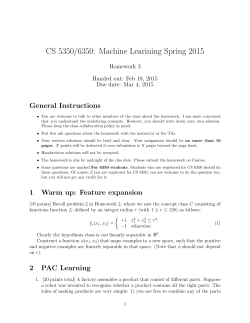
Fig. 1. Different mobile robot outdoor platforms with different capabilities
and different fields of applications.
into designing the model for the traversability analysis for a
specific platform, with a specific sensor setup. This is often a
time consuming and costly process. It would be much easier
if one could just steer the robot manually in the environment
to train the traversability analysis. But to make use of this
data, the problem is that the learning algorithm only gets the
information of the traversed part during the training. This
means that the training set contains only incomplete positive
labels and no negative information. In our approach we adapt
learning algorithms for that kind of problem to a frame work
that makes it possible to infer the traversability analysis for
the mobile robot.
II. R ELATED W ORK
Recently, Papadakis published a survey of traversability analysis methods for unmanned ground vehicles [14].
It states that the predominant approaches to measure
traversability are based on occupancy grid maps, which
are accredited to Moravec and Elfes [11]. More concrete,
they are based on the analysis of 2d elevation maps, where
3d information is represented in 2d maps. Pfaff et al.
presented an approach, where the 2d elevation maps were
used for traversability analysis as well as for mapping and
localization purposes [16]. A more general representation
is a 2d grid map, where each cell stores features that
provide enhanced information from the senors. Papadakis
identified this as the preferred choice when dense 3d point
clouds are available [6, 7, 8]. Our approach also uses this
kind of 2d grid map, where each cell is associated with
at least one feature vector that is computed from the 3d
points that are mapped to the respective cell. Many methods
to perform traversability analysis are based on heuristics
that represent the capabilities of the robot, in combination
with measurement models that describe the sensor noise
[2, 3, 7]. These methods to classify traversability typically
work well for many environments, but they are limited in
their generality, since they often do not explicitly distinguish
different types of obstacles, like rocks or grass. Moreover,
a specific heuristic has to be developed for every robot
and also for different combinations of sensors and terrain.
Murphy and Newman use a probabilistic costmap, which is
generated from the combined output of a multiclass gaussian
process classifier and gaussian process regressors. It models
the spatial variation in cost for the terrain type, to perform
fast path planning, taking the uncertainty of the terrain cost
into account [12].
Another problem which is hard to tackle are the so called
negative obstacles, like holes in the ground or downwards
leading steps. The sensor is not necessarily able to perceive
the lower part of the structure and therefore the robot has to
reason about the cause for missing data, which might result
from untraversable gaps or simple visibility issues [10, 18].
This is of special interest in search and rescue scenarios
after disasters, where the environment is very complex due to
irregularities. This kind of analysis is especially critical when
the sensors that are used only provide a sparse representation
of the environment, like rigidly mounted, downwards facing
2d-laser scanners.
A natural thing would be to let the robot learn about the
traversability of the environment. This has the advantage that
there is no need for a heuristic to interpret the senor data.
But in supervised scenarios one has to provide labeled data
to the approach to learn from. Lalonde et al. [9] proposed to
segment 3d point clouds into the categories scatter, to represent porous volumes, linear, to capture, e.g., wires and tree
branches, and surface to capture solid objects like ground
surfaces. The authors achieve this by training a Gaussian
Mixture Model with an expectation maximization algorithm
on hand labeled data. A different way to perceive the
environment is to use proprioceptive measures, like bumper
hits, measuring slip, or vibration. Those can be combined
with geometric measures and used, e.g., to project the current
measurements into the environment [1, 6, 17]. Yet, the use of
proprioceptive measures requires an adequately robust robot
that is physically able to traverse the terrain in question. Even
though such methods allow the robot to autonomously learn
a model of the environment, the trial and error part of this
methodology involves a high risk to damage the robot.
In contrast to this, our approach uses data collected
from a human operator that drove a safe trajectory and
therefore provided partially labeled training data. This is
a very convenient, safe, and time efficient way to train
a classifier. An approach that follows a similar idea was
presented by Ollis et al. [13]. Their system uses data from
a stereo camera, radar, as well as 2d- and 3d-lidar sensors.
Features are computed as multidimensional histograms and
a distribution is learned for the traversed cells. The approach
makes use of a monotonicity assumption that states that cells
with higher values of the features would be expected to be
less traversable and the inferred probabilities were enforced
to meet this assumption. The resulting values are mapped to
a cost function that is then used for planning.
In our approach there are no heuristic assumptions about
the features and their relation to the traversability. To solve
this special learning problem, we adapted the work of Denis
et al. [4] and Elkan and Noto [5] to learn the probabilities
from the available data.
III. BASIC S TRUCTURE
For our approach, we interpret traversability as a local and
static characteristic of the environment. We use a mobile
robot equipped with a 3d-lidar sensor that also provides
remission values of the measurements, which we assume
to be calibrated. Since we interpret the characteristic of
traversability to be static, we further assume that dynamic
objects are detected and removed in advance. The map representation we use is a 2d occupancy grid G with resolution
r ∈ R>0 , where each cell can hold one or more feature
vectors. The perceived 3d-points are mapped to the grid cells
by projection and after a covered distance of dP ∈ R>0 we
compute and add a feature vector from the points in the cell.
This feature vector is composed of geometrical measures
and the remission values. By discretization of the feature
vectors, using fixed size increments, we create a Vocabulary
V of discrete features. We expect those features to be
multinomial distributed given the traversability state of a cell,
P (. | state) ∼ Multinomial with state ∈ {trav , ¬trav }.
Therefore the goal of our approach is to learn the parameters
for that distribution in order to calculate P (trav | f1 , . . . , fn )
for fi ∈ V. To avoid accumulated registrations errors, we use
only local maps that are used for a distance of dM ∈ R>0 ,
which is a typical workaround to avoid global inconsistencies
of the registration process.
IV. T HE L EARNING P ROBLEM
One of the goals of our approach is that it can be
used by humans that are not especially educated to design
traversability models for mobile robots. We achieve this by
designing a naive method for generation of training data.
More concrete, the training data is generated by a human
that operates the robot in an environment that is similar
to the environment where the robot should later be able to
reliable operate in. From this training trajectory, the cells that
intersect with the projection of the footprint of the robot are
labeled as positive examples. Using this process for training
data generation has the advantage that it is fairly easy to
execute but also has the drawback that we get only scarce
positive examples and tons of unlabeled data to learn from.
Fortunately this kind of data is a very common problem
in, e.g., text classification and biological approaches like
protein categorization and we can adapt existing methods
for our approach. We use and compare two strategies to
learn a classifier from this kind of training data, one called
Fig. 2. Trajectory of Robot1 on the forest track that was used for the
c Google)
experiments on an aerial image (
Positive Naive Bayes (PNB) introduced by Denis et al. [4]
and Learning Classifiers from Only Positive and Unlabeled
Data (POS) by Elkan and Noto [5]. The former one was
developed for text classification, where this kind of data is
very common, and also assumes the words to be multinomial
distributed. The latter one is a more general approach that
can deal with a variety of distributions.
A. Feature Design
In feature based approaches, it is important that the
features are designed to capture the world for the intended
task. For our approach this means that they should be able
to distinguish obstacles from traversable ground for different
platforms. They have to distinguish flat solid ground from
moderate steps, between many kinds of vegetation and from
solid obstacles of certain heights, since it depends strongly
on the robot, if these are traversable or not. For our approach
we use feature vectors that contain the following measures.
•
•
•
•
•
The
The
The
The
The
absolute maximum difference in the z-coordinate
mean of the remission values
variance of the remission values
roughness of the cell
slope
Each dimension should help to distinguish different types
of terrain as well as traversability constraints of the robot.
The maximum height difference and the slope reflect the
ground-clearance of the robot as well as the motor power.
The remission values and the roughness help to distinguish
concrete and vegetation types. Since the calculation of the
first three dimensions is straight forward, we shortly explain
the calculation of the latter two, which are based on the
eigenvalues and the respective eigenvectors of the covariance
matrix of the points in the cell. The smallest eigenvalue is
used as a roughness parameter. The eigenvector that belongs
to the smallest eigenvalue is used as the normal vector of
the cell, and the slope is the angle between the normal and
the vector of gravity. To ensure that these values are well
defined, we ignore cells that contain less than five points.
c Google) with the training (blue) and evaluation
Fig. 3. Aerial image (
(red) trajectory of Robot2 on the Campus.
B. Positive Naive Bayes
The Positive Naive Bayes Classifier, as introduced by Denis et al. [4], estimates the frequencies of observed features
in the classical way. Since the data is only incompletely
labeled and contains no negative labeled samples, it calculates an estimate for the negative frequencies from the
previous estimate of the positive frequencies and the prior.
In particular, let the set P D contain all the positive labeled
cells including their observations and U D be the set of the
unlabeled cells. Let C : V × 2G → N be the counting
function,
P
P i.e., for S ⊂ G, f ∈ V we define C(f, S) :=
c∈S
fc ∈c 11f (fc ), whereatP11 is the indicator function.
Further we define C(S) :=
f ∈V C(f, S) as the number
of observations, including multiplicity, in the set S. The
probability given the positive class, which means in our case
the traversable class, is estimated by:
P (f | trav ) =
αp + C(f, P D)
αp |V| + C(P D)
Where αp ∈ [0, 1] is the additional smoothing parameter,
which was in our case set to αp = 1/|V|. To estimate
the probability given the negative class is a little bit more
complicated, due the problem that no negative examples are
available. Therefore we substitute the counting function with
CN (f ) := max{C(f, U D) − P (f |trav )P (trav )C(U D); 0}
With this approximate counting function we estimate the
probability for a feature given the negative class.
P (f | ¬trav ) =
αn + CN (f )η
αn |V| + (1 − P (trav ))C(U D)
Where η is the normalizer for the not smoothed probability
using CN (f ). For the negative class we used the smoothing
factor αn = 1. The reason for using different values for
αp and αn is that if we observe a feature that was never
observed before, we would get P (f | trav ) > P (f | ¬trav )
since in our case C(P D) << (1 − P (trav ))C(U D). This
would result in a positive classification for a cell that contains
only unseen features, which is incompatible with the safety
requirements for traversability analysis. We finally compute
P (trav | f1 , . . . , fn ) using Naive Bayes.
Aerial image
Ground truth
PNB-based classifier
POS-based classifier
Fig. 4. Traversability map from the forest run with Robot1 using our approach. From left to right: Aerial image of the scene, ground truth labeled
map which was used for the evaluation, our approach using the PNB-based classifier and our approach using the POS-based classifier. The grass on the
mid-upper left side is correctly labeled as traversable (green) while the parts of the forest are labeled as obstacles (red). The POS-based classifier has false
positives in the lower left and mid right. Both classifiers have problems with the measurements at the border of the map.
C. Learning from Positive Only
The classifier that is proposed in the work of Elkan and
Noto [5] follows a different strategy. In their work they
use the sets P D and U D to estimate the distribution for a
feature f to get a label (always positive) during the training,
P (label | f ), f ∈ V. This is now a classical learning
problem with full labeled data, since we know for each
feature whether it got a label or not. Once the distribution of
P (label | f ) is estimated, Elkan and Noto elaborated a way
to transfer this to P (trav | f ). Elkan and Noto proofed, that
given the selected completely at random assumption there
exists c > 0 such that P (trav | f ) = P (label | f )/c.
While they provide different ways to estimate c using a
validation set, we use the maximum estimate for c, since
it should be the most conservative one. Nevertheless, since
we have only incomplete data, it is still possible that for
some features P (label | f ) > c. To cope with such cases
we set P (trav | f ) = min{P (label | f )/c ; (1 − )}. In
our approach we train the distribution P (label | f ) using
standard Naive Bayes using the same smoothing parameters
as described in Sec. IV-B. We use the efficient log-odds
update to integrate multiple measurements within one cell,
utilizing the static map assumption.
logodds(trav | f1 , . . . , fn ) = logodds(trav |fn )
+ logodds(trav | f1 , . . . , fn−1 )
+ logodds(trav )
D. Terrain Models
Since the learning algorithms only get the positive data of
the trajectory the unlabeled data may also contain features
of a different type of terrain that is traversable. The learning
algorithms may get confused if we merge all the data within
one distribution. For example if during the training we
traverse most of the time the street and only a short time
grass, then the ratio of labeled grass data is very small
and therefore the learning algorithms can not adept grass to
be traversable. This kind of problem will occur whenever
the training set of the terrain types is not balanced. For
the method described in Sec. IV-C it will also violate the
selected completely at random assumption. To overcome
this problem we use a set of different terrain models M.
The positive examples of a local map are compared to the
existing terrain models using Pearson’s χ2 -test, [15], with a
significance level of α = 0.05. If the test cannot discard the
null hypothesis, we merge the data of the local map with
the respective model. Otherwise, if the test discards the null
hypothesis for all existing models, a new model is added to
M. For the method described in Sec. IV-B we use a one-vsall strategy for the final classifier.
P (trav | f1 . . . , fn ) = max Pm (trav | f1 , . . . , fn )
m∈M
For the method described in Sec. IV-C we need to specify
how to compute P (trav | f ) in the context of terrain models.
We use a featurewise one-vs-all strategy here.
P (trav | f ) = max Pm (trav | f )
m∈M
E. Training
The training phase is fairly easy for the user. The robot is
operated by a human over all kinds of terrain it can traverse.
During this phase the local maps are given to the learning
algorithm. Then the statistic test is computed for the terrain
models. Afterwards the selected model, it may be an existing
one or a new one, is merged with the data from the local
map and the current distribution of the models are computed.
More formal, for a selected model m ∈ M the set of labeled
data becomes P Dm = P Dm ∪ P Dl and the set of unlabeled
data becomes U Dm = U Dm ∪ U Dl . This sequential structure of our learning strategy also allows to retrain the robot
at any point in time. This might be interesting for scenarios
where the robot acts mainly autonomous but is connected to
a command center where it can put requests if for example
it can not find a path to the mission goal.
BOTH
FOREST
CAMPUS
BOTH
FOREST
CAMPUS
0.93
0.91
0.89
0.87
0.85
0.83
0.81
0.79
0.77
0.75
Specificity
A. Evaluation with Robot1
We trained Robot1 on the Campus, by driving over grass
of different heights and with different flowers, dirt, walkways
and streets. For the evaluation of our classifier we use a test
track containing dirt roads, Fig. 2, and on the campus where
we traversed walkways as well as grass areas. For the quality
measures of the classifiers we labeled 30 local maps from
the forest track and 5 from the campus track, which is about
10% of the local maps that were created during the run. The
ground truth was labeled rather conservative, i.e., especially
in forest environment the cluttered areas between the trees
were hard to classify for each and every cell, in doubt
they were classified as not traversable, since the measure of
false positives is more important for traversability analysis.
Nevertheless, a false positive was counted if and only if the
inspected cell and all eight adjacent cells were classified as
positive (traversable). In this experiment our approach shows
better results, in terms of precision and specificity, when we
use the PNB-based classifier than with the POS-based classifier. On the combined data set, with the full feature vector,
the PNB-based classifier reaches 0.992 while the POS-based
classifier has 0.945. The POS-based classifier has problems
especially with the forest data, 0.990 vs. 0.934, while this
difference is not that substantial for the campus data set,
0.998 vs. 0.990. It is interesting to notice that for the PNBbased classifier the remission values (0.990 for NoRe) seem
not to be as important as the roughness and slope (0.953 for
NoRS) values. This role changes for the POS-based classifier
where the precision without remission is worse than without
roughness and slope. For both classifiers the full feature
vector is superior to the pruned feature vectors. As expected
the performance for the recall is antithetic to the precision.
1
0.99
0.98
0.97
0.96
0.95
0.94
0.93
0.92
0.91
0.9
0.89
0.88
0.87
0.86
0.85
0.95
Recall
In the experiments, we used two mobile robots with
different capabilities, like in Fig. 1. One robot is capable
of urban as well as outer urban environments, providing
good motor power, high ground clearance and good stability
(Robot1). The other is only capable of urban environments,
with small ground clearance and weak stability (Robot2). On
both platforms we evaluate the quality of the classification
using hand labeled ground truth on suitable test tracks,
e.g., Fig. 2 and Fig. 3. Furthermore we compare the quality
of the classifier when we omit the remission values (NoRe)
and when we omit the roughness and slope values (NoRS)
of the feature vector, see Sec. IV-A. For the experiments we
used dM = 20m, dP = 0.5m and limited the maximum
range of our 3d-lidar sensor to 20m. We used the same
parameters to discretize the feature vectors for both robots.
Consecutive local maps were used to train and evaluate the
classifiers. Cells were classified as traversable if and only
if P (trav | f1 , . . . , fn ) > 0.5. Dynamic Obstacles were
removed from the scans using an online dynamic obstacle
detection approach based on scan differencing. The point
clouds are registered using an Applanix Navigation System.
The robots are equipped with 3d-lidar sensors from Velodyne,
providing 360◦ horizontal and ∼ 30◦ vertical field of view.
Precision
V. E XPERIMENTS
1
0.98
0.96
0.94
0.92
0.9
0.88
0.86
0.84
0.82
0.8
0.78
0.76
0.74
0.72
0.7
PNB
BOTH
PNB-NoRe
PNB-NoRS
FOREST
POS
CAMPUS
POS-NoRe
POS-NoRS
Fig. 6.
Precision, Recall and Specificity for the test trajectories of
Robot1. We compare the performance of the full feature vector, without
remission values (NoRe) and without roughness and slope values (NoRS).
The classifier based on PNB is shown in blue and the one based on POS in
orange. For both methods using the full feature vector improves precision
and specificity, the role of remission values and roughness and slope values
behave different for the two methods.
In this measure the POS-based classifier, 0.87, is superior
to the PNB-based classifier, 0.79. Like for precision this
difference is larger on the forest data set than on the campus
data set. The last quality measure we used in our evaluation
is the specificity, see Fig. 6 bottom. This measure is of great
importance, since it measures the rate of the true negative
classifications. A Type I Error means wrong classification of
a negative sample. In the case of traversability analysis this
means missing an obstacle. Here again, already indicated
by the precision measure, the PNB-based classifier, 0.987,
is superior to the POS-based classifier, 0.898. While we
observed different gaps between the classifiers for precision
and recall on the forest and campus data set, measuring the
Aerial image
Ground truth
PNB-based classifier
POS-based classifier
Fig. 5. Traversability map from the campus run with Robot2 using our approach. From left to right: Aerial image of the scene, ground truth labeled map
which was used for the evaluation, our approach using the PNB-based classifier and our approach using the POS-based classifier. Both classifiers produce
similar results.
TABLE I
E VALUATION FOR ROBOT 2 ON THE CAMPUS TRAJECTORY.
POS
PNB
Method
Measure
Precision
Recall
Specificity
Precision
Recall
Specificity
Full
0.978
0.947
0.984
0.975
0.947
0.982
NoRe
0.924
0.868
0.945
0.637
0.940
0.589
NoRS
0.958
0.954
0.967
0.840
0.961
0.859
Results for Robot2 on the campus trajectory (Fig. 3). Both learning
methods behave quite similar in this scenario when using the full feature
vector. The absence of roughness and slope measures (NoRS) gives a
better performance in this scenario than the absence of remission values
(NoRe).
specificity the difference is roughly the same for both data
sets. Note that the results of this experiment do not prove that
the PNB method is in general superior to the POS method,
but for this data set and the way we use it.
B. Evaluation with Robot2
For Robot2 we used only a short training trajectory on the
campus, see the blue part of Fig. 3, since the complexity of
the environment is much lower than for the forest data set.
In this environment both classifiers perform almost identical
with the full feature vector, see Tab. I. Both the classifiers
reach the precision of 0.98, recall of 0.95 and specificity of
0.98. In this scenario the remission values are more important
than the roughness and slope parameters. Using the POSbased classifier the precision without remission values is 0.63
and without roughness and slope it is 0.84. Especially for the
POS-based classifier the combination of both improves the
performance substantially, while for the PNB-based classifier
the performance is similar.
VI. C ONCLUSION
We presented an easy to use approach to learn traversability for mobile robots. In the experiments we showed that our
approach can be applied to different robots with different
traversability characteristics. Moreover, our approach is usable in outdoor urban environments as well as in unstructured
non-urban environments like forest roads and grassland.
R EFERENCES
[1] A. Angelova, L. Matthies, D. Helmick, and P. Perona. Learning and
prediction of slip from visual information. Journal on Field Robotics,
2007.
[2] I. Bogoslavskyi, O. Vysotska, J. Serafin, G. Grisetti, and C. Stachniss.
Efficient traversability analysis for mobile robots using the kinect
sensor. In European Conference on Mobile Robots (ECMR), 2013.
[3] G. Broten, D. Mackay, and J. Collier. Probabilistic obstacle detection
using 2 1/2 d terrain maps. In Computer and Robot Vision (CRV),
2012 Ninth Conference on, 2012.
[4] F. Denis, R. Gilleron, M. Tommasi, et al. Text classification from
positive and unlabeled examples. In Proceedings of the 9th International Conference on Information Processing and Management of
Uncertainty in Knowledge-Based Systems, IPMU’02, 2002.
[5] C. Elkan and K. Noto. Learning classifiers from only positive
and unlabeled data. In Proceedings of the 14th ACM SIGKDD
international conference on Knowledge discovery and data mining,
2008.
[6] A. Howard, M. Turmon, L. Matthies, B. Tang, A. Angelova, and
E. Mjolsness. Towards learned traversability for robot navigation:
From underfoot to the far field. Journal on Field Robotics, 2006.
[7] D. Joho, C. Stachniss, P. Pfaff, and W. Burgard. Autonomous
exploration for 3D map learning. In Fachgesprche Autonome Mobile
Systeme (AMS).
[8] S. Kuthirummal, A. Das, and S. Samarasekera. A graph traversal based
algorithm for obstacle detection using lidar or stereo. In IEEE/RSJ
Int. Conf. on Intel. Rob. and Sys. (IROS), 2011.
[9] J.-F. Lalonde, N. Vandapel, D. F. Huber, and M. Hebert. Natural
terrain classification using three-dimensional ladar data for ground
robot mobility. Journal on Field Robotics, 2006.
[10] J. Larson and M. Trivedi. Lidar based off-road negative obstacle
detection and analysis. In Intelligent Transportation Systems (ITSC),
2011 14th International IEEE Conference on, 2011.
[11] H. P. Moravec and A. Elfes. High resolution maps from wide angle
sonar. In IEEE Int. Conf. on Rob. & Aut., 1985.
[12] L. Murphy and P. Newman. Risky planning on probabilistic costmaps
for path planning in outdoor environments. Robotics, IEEE Transactions on, 2013.
[13] M. Ollis, W. H. Huang, and M. Happold. A bayesian approach to
imitation learning for robot navigation. In IEEE/RSJ Int. Conf. on
Intel. Rob. and Sys. (IROS), 2007.
[14] P. Papadakis. Terrain traversability analysis methods for unmanned
ground vehicles: A survey. Engineering Applications of Artificial
Intelligence, 2013.
[15] K. Pearson. X. on the criterion that a given system of deviations from
the probable in the case of a correlated system of variables is such that
it can be reasonably supposed to have arisen from random sampling.
The London, Edinburgh, and Dublin Philosophical Magazine and
Journal of Science, 1900.
[16] P. Pfaff, R. Triebel, and W. Burgard. An efficient extension to elevation
maps for outdoor terrain mapping and loop closing. Int. Jour. of Rob.
Res., 2007.
[17] M. Shneier, T. Chang, T. Hong, W. Shackleford, R. Bostelman, and
J. S. Albus. Learning traversability models for autonomous mobile
vehicles. Autonomous Robots, 2008.
[18] A. Sinha and P. Papadakis. Mind the gap: detection and traversability
analysis of terrain gaps using lidar for safe robot navigation. Robotica,
2013.