
Do Public Health Interventions Crowd Out Private
Do Public Health Interventions Crowd Out Private Health Investments? Malaria Control Policies in EritreaI Pedro Carneiroa , Alex Armandb , Andrea Locatellic , Selam Mihreteabd , Joseph Keatinge a Department of Economics, University College London, Gower Street, WC1E 6BT, London, UK, Institute for Fiscal Studies, CeMMAP ([email protected]) b University of Navarra, NCID - Edificio de Bibliotecas, 31009 Pamplona, Spain ([email protected]) c Economic Research Unit, Bank of Italy, Bolzano branch, via Orazio 1/E, 39100 Bolzano, Italy ([email protected]) d National Malaria Control Program, P.O. Box 212, Ministry of Health, Asmara, Eritrea ([email protected] ) e Department of Global Health Systems and Development, Tulane University School of Public Health and Tropical Medicine, 1440 Canal Street, Suite 2200, New Orleans, La 70112 USA ([email protected]) Abstract It is often argued that engaging in indoor residual spraying (IRS) in areas with high coverage of mosquito bed nets may discourage net ownership and use. This is just a case of a public program having perverse incentives. We analyse new data from a randomised control trial conducted in Eritrea which surprisingly shows the opposite: IRS encouraged net acquisition and use. Our evidence points to the role of imperfect information. The introduction of IRS may have made the problem of malaria more salient, leading to a change in beliefs about its importance and to an increase in private health investments. I This research collaboration was initiated under Development Impact Evaluation’s (DIME’s) Malaria Impact Evaluation Program. We would like to thank especially Arianna Legovini and Edit V. Velenyi for their role in client engagement, research design, and securing funding for the study. We would also like to thank officials at the Eritrean Ministry of Health, the National Malaria Control Program and the data collection team at the Orotta School of Medicine in Asmara. Without them this research would not have been possible. This research was funded by a World Bank grant (as part of the HAMSET II project) through the Project Management Unit of the Eritrea Ministry of Health and a World Bank grant from DIME. We thank Achyuta Adhvaryu, Noel Chisaka, Jean-Paul Clark, Pascaline Dupas, Costas Meghir, Petra Todd and seminar participants at UCL, IFS, the AEL Conference 2011, the 10th Arnoldshain Seminar, DIME-World Bank, PSE, Uppsala, NOVAfrica, Centre for Global Development, and NEUDC Conference 2011 for helpful comments. Carneiro gratefully acknowledges the financial support from theWorld Bank, the Economic and Social Research Council for the ESRC Centre for Microdata Methods and Practice (grant reference RES589-28-0001), the support of the European Research Council through ERC-2009-StG-240910-ROMETA and ERC-2009-AdG-249612, and the hospitality of the World Bank Research Group. Preprint submitted to Elsevier 16th March 2015 Keywords: Malaria, Bed nets, Indoor Residual Spray, Information, Beliefs, Behaviour. JEL: D12, D83, H42, I12. 1. Introduction Most public programs induce behavioural responses in their target population. These responses are often perverse, making programs less effective than what was originally intended. This is a central concern in the design of public interventions across a variety of areas, in rich and poor countries alike. In the particular case of malaria control programs, the introduction of indoor residual spraying1 (IRS) could have a negative impact on the use of insecticide treated mosquito bed nets (ITN), if individuals believe IRS and ITN as substitutes in the prevention of malaria (e.g. Lengeler, 2011). In the standard model, the extent to which private investments crowd-out public investments depends on the degree of substitutability between the two. However, outside the scope of this simple model are situations where the introduction of a program changes the information set of individuals. For example, by introducing a health program in a community, the public health authorities may be perceived to be especially concerned about that particular health problem. This may then indicate to individuals that the problem may be more serious than what they initially perceived it to be, inducing a change in their beliefs about the returns to private health investments. A program could have an implicit information component even when it does not include an explicit information campaign. In this context, the standard crowding-out intuition breaks down and an increase in public health investments can lead to an increase in private health investments even when they are substitutes.2 1 Indoor residual spraying consists in spraying the interior walls of dwellings with insecticide to kill resting mosquitoes. 2 Some public reaction in the US to the recent Ebola outbreak has some similarities with the situation we just described. There is limited public information about Ebola, which means that public perceptions of the disease may be easier to change than in cases where there is a higher level of knowledge. The perception of massive government investments towards the prevention of Ebola in the US (both in the countries where the outbreak originated from and in the US), may have lead some individuals to become very worried about the possibility of an Ebola outbreak in the US. This change in perceptions lead individuals to act accordingly, either through their own health behaviours or by putting pressure on the politicians who represent them. 2 Although this is a simple point, and potentially relevant for many education and health programs in developing countries, it is often ignored. This paper presents experimental evidence from Eritrea that an IRS campaign led to increases in ITN ownership and use. Our analysis suggests that the introduction of IRS may have made the problem of malaria more salient in treatment villages, causing a change in beliefs about the importance of the disease in these areas, which resulted in an increase in private health investments. The data used in our study comes from an experimental evaluation of the impact of an IRS program organised by the Government of Eritrea in the most malarious region of Eritrea (Gash Barka). Fifty-eight (58) villages were randomly assigned to treatment and 58 villages were randomly assigned to control. Between June and July 2009, before the start of the malaria season, households in treatment villages were visited by government workers carrying IRS equipment and were offered free IRS3 . Households in control villages did not receive publicly provided IRS and, at the same time, IRS is not privately provided in this market. A household survey and malaria rapid diagnostic tests (RDT) were administered during the malaria season that followed (October 2009). The prevalence of malaria parasite infection was found to be very low in this area, and our data shows that IRS had no detectable impact on it (Keating et al., 2011). However, it led to higher ownership and use of ITNs, in a setting where IRS and ITN are more likely to be perceived as substitutes rather than complements. In addition, households in treatment villages became more aware of (and concerned with) malaria than in control villages. In particular, they were more likely to mention mosquitoes as a malaria vector and to mention children as one of the groups most affected by malaria, than households in control villages. A large literature debates the extent to which a variety of public programs discourages (or crowds-out) private investments in those goods or services that are provided by the public sector. Two examples (among many) are Peltzman (1973), who discusses the case of higher education in the US, and Cutler and Gruber (1996), who study health insurance in the US. Examples of the importance of crowding-out effects for health programs in 3 Teams visiting villages for IRS treatment were composed by social workers. It is unlikely in this situation that IRS teams provided information about malaria, in addition to offering IRS treatment, to the households living in treated villages. Within the National Malaria Control Program, information campaigns are managed by a communication team, which did not participate in the IRS campaign. 3 developing countries are much less common in the literature than for developed countries, perhaps because of lack of data. Some examples include Das et al. (2011), who analyse education subsidies in Zambia and India, and Bennett (2012), who studies the negative effect of the provision of piped water on household sanitary behaviour in the Philippines. The standard presumption in these papers is that there is substitutability between private and public expenditures, say, in health, and that individuals have perfect information about the returns to their health investments. However, there is increasing evidence that decisionmaking by the poor is greatly affected by limited information (e.g. Bertrand et al. 2006; Banerjee and Duflo 2011; Dupas 2011b). This means that health programs have the potential to simultaneously deliver health services and induce changes in beliefs about the returns to health investments in the populations they serve, which could even lead to a reversal of potential crowding-out effects. Beyond the literature on crowding-out effects of public programs, it is also important to mention how our study fits into the literature on malaria control programs and on information and health in developing countries. Providing information about the returns from using a technology can be an effective way to promote both take-up and use. Dupas (2011b) reviews several studies that show how the provision of information can effectively influence people’s health-seeking behaviour, when they are not already fully informed about the health situation they face, when the source of information is credible and when they are able to process the new information. In other words policies may affect people’s behaviour if they are able to change their beliefs. In a study of HIV in Malawi, De Paula et al. (2011) do not find strong evidence that HIV testing consistently affects people’s beliefs about their own HIV status (see also Delavande and Kohler, 2009), but they also show that downward revisions in beliefs about HIV status increase risky behaviour, while the opposite occurs with upward revisions. In another study about HIV-related behaviour, Dupas (2011a) shows that providing information on the relative risk of HIV infection disaggregated by gender and age has a significant effect on teenage pregnancy. The role of information in public health program and health behaviour in developing countries is also key in Madajewicz et al. (2007); Goldstein et al. (2008); Kremer et al. (2009). Therefore, it is important to recognise how the availability of information about the benefits of using one technology plays a central role in public health policies. Borrowing 4 from the literature in marketing and psychology, Dupas (2009) analyses how the framing of information on the benefits of ITN use affects ownership and use of ITNs. She compares two cases: one which stresses the financial gains from a reduction in missed work and another highlighting the health gains from avoiding malaria. Using data from a randomised control trial (RCT) from Kenya, Dupas finds that neither take-up nor usage are affected by how benefits are framed in a marketing campaign. As a possible explanation, she proposes that the stakes are high and that liquidity constraints are probably the main barrier to investments in malaria prevention. We also contribute to the understanding of ITN use, which is the main tool available to households to prevent malaria infection. Several studies have investigated ways to promote acquisition and usage of ITNs in malarious villages and attention has been focused on the comparison between free-distribution and cost-sharing programs. One central paper on this topic is that by Cohen and Dupas (2010), who provide evidence in support of free distribution. This aspect is further investigated by Tarozzi et al. (2013), who conducted a RCT in Orissa (India) and provided evidence on the effectiveness of micro-loans promoting ITN ownership. Finally, the way nets are used within household is investigated by Hoffmann (2009), who, using a RCT in Rural Uganda, shows that, under free distribution of nets, households tend to allocate them to specific members and, in that particular setting, to children younger than 5 years old. The remainder of the paper is organised as follows. In Section 2 we briefly describe the study area and the status quo in malaria eradication. In Section 3 we describe our dataset and we introduce our model in Section 4. We present and discuss our estimates in Section 5. Section 6 concludes. 2. IRS in Eritrea and the Intervention Malaria is transmitted to humans, mainly at night, from the bite of infected female mosquitoes. Three main technologies are currently used to reduce transmission: ITNs, larval habitat management (LHM) and IRS. ITNs must be hung over the bed at night to protect sleeping individuals from infectious mosquito bites; LHM includes activities such as destroying the habitat of mosquitoes by draining stagnant water; IRS consists of spraying the inside walls of dwellings with insecticide to kill resting mosquitoes. 5 Eritrea has been successful in greatly reducing malaria prevalence to relatively low levels. Malaria dramatically declined in the country over the past decade, from a national peak of 260,000 clinical cases diagnosed in 1998 to just under 26,000 cases in 2008.4 In Eritrea, the costs of IRS are borne almost exclusively by the Government, which conducts spraying campaigns (there is no private market for IRS activities). Similarly, LHM campaigns are organised out by the Government with the active involvement of local populations. In contrast, ITNs must be acquired by individuals and then set up above the bed. There exist periodic massive distribution campaigns for ITNs, but use and care of ITNs is still a private decision. Sleeping under a net is perceived as unpleasant, especially in warm weather, and ITNs also need regular re-impregnation, if they are not coated with long lasting insecticide.5 IRS is an expensive intervention, although generally perceived as effective. Nevertheless, there are no studies of the added benefit of IRS in low-transmission settings over and above ITN use, effective case management and LHM. As such, the National Malaria Control Program (NMCP) decided to conduct an evaluation of the impact of IRS in the context of the existing control program (which promotes LHM and ITN use) with the support of the World Bank. The results of this evaluation are presented in Keating et al. (2011). The intervention was conducted in the Gash Barka region6 , one of the six zones that compose the country and the most malarious zone in Eritrea. This zone registered more than half of all diagnosed malaria cases and over 60 percent of all related deaths in the country, for the years of 2007 and 2008. The location of the zone is shown in Figure B1. Gash Barka is mostly a rural/agricultural area, inhabited by one fifth of the country’s population, which is estimated at 3.6 million. Altitudes range between 500 and 1,500 4 The information about Malaria clinical cases is provided by the Eritrean National Malaria Control Program (NMCP). 5 There is limited evidence on the barriers to mosquito net use in malaria-endemic regions (Pulford et al., 2011). However, discomfort, mainly related to heat, is among the main identified reasons for not using the nets. 6 Gash Barka is composed by 14 sub-zones: Akurdet, Barentu, Dighe, Forto, Gogne, Goluj, Haykota, Laelay-Gash, Logo Anseba, Mensura, Mogolo, Mulki, Shambko and Tesseney. We surveyed only 13 of those sub-zones, because one of the sub-zones, Logo Anseba, was deemed to have a very low malaria prevalence attributable to higher altitude. 6 meters and temperatures are generally associated with hot and dry climatic conditions. Significant variation can be observed across the region in terms of precipitations, leading to marked differences in vegetation and malaria prevalence. The rainy season is concentrated between July and September, while precipitations are scarce during the rest of the year. As a result, malaria transmission is higher in the period from July to December, with a peak in September and October, following the rainy season. A two-arm cluster-randomised controlled trial (using a post-test only design) was used to evaluate the impact of IRS on malaria infection prevalence. Effectiveness was measured as a single difference between treatment and control groups. One hundred and sixteen (116) villages in Gash Barka were selected for the study. Fifty-eight (58) villages were randomly assigned to the treatment group and 58 villages were randomly assigned to serve as the control group. A geographic buffer was used to insure that treatment and control villages were at least 5 km apart. The NMCP verified the distance between treatment and control villages, and villages that were within 5 km from another were replaced by the closest village at least 5 km apart. In addition, further replacements were made in a few cases where the originally chosen village had moved and could not be found or reached. Again, the closest eligible village was chosen as a replacement.7 In each treatment village, the intervention involved the control of adult mosquito populations using IRS with the insecticide dichlorodiphenyltrichloroethane (DDT), which is recommended by the Eritrean NMCP. During the months of June-July 2009, dwellings were sprayed according to the manufacturer’s recommended guidelines. The spraying targeted all households to ensure a minimum coverage of 80 percent, as recommended by the World Health Organisation (WHO). Treatment and control villages received similar levels of ITNs, LHM and case management, per existing NMCP guidelines and policy. Further details on the study design and intervention are available in Keating et al. (2011). 7 This procedure is documented in detail in the Online Supplementary Material that describes the procedures followed for treatment allocation. 7 3. Data A household survey was conducted in October 2009,8 which corresponds to the period right after the peak of the malaria season. Only one person per household was interviewed and the response rate was high at 94.23 percent, yielding a total sample size of 1,617 households (corresponding to 7,895 individuals), of which 809 lived in treatment villages and 808 resided in control villages. All present and consenting household members were tested for malaria using Carestart® RDTs and microscopy was used to validate positive RDT results.9 Tables 1 and 2 present means and standard deviations for variables which are essentially pre-determined, and mean differences between the treatment and the control groups. Even though some of these variables could potentially respond to the intervention, it is unlikely that any response along these dimensions (household demographics and dwelling characteristics) took place between the time of the intervention (June-July 2009) and the time of the survey (October 2009). Table 1 shows individual-level variables and Table 2 shows household-level variables. All the characteristics of treatment and control villages are balanced with one exception: the Tigre tribe is over represented in the treatment group. We take this into account in our analysis by including in all regressions an indicator variable that takes a value equal to 1 if household i belongs to the Tigre tribe and 0 otherwise. The exclusion of this variable does not affect our results. Tables 1 and 2 also show joint tests that check the balance of several variables simultaneously. We consider three different sets of variables: those available for the whole sample, those available for respondents only and those available only at the household level. To conduct the test we run probit regressions of treatment assignment on the variables in each group and we test whether the coefficients in the regressions are jointly equal 8 A baseline survey was not collected because of budgetary constraints. Appendix C provides a detailed description of the data and of all the variables used in this paper. 9 A total of 5,502 people were tested with RDT. 1,120 people were absent at the time of the survey and they could not be tested. In addition, 651 people refused testing. Among those tested, 13 individuals tested positive in the control group and 17 tested positive in the treatment group. The difference between the share of positive RDTs in the two groups is 0.001 (st. err. = 0.003) and not significant (see Keating et al. 2011). Malaria prevalence was (unexpectedly) very low in the area under investigation. No other additional test, such as anaemia, was collected. 8 to zero. To be precise, let Ti denote an indicator that takes value 1 if household i belongs to a treatment village and 0 otherwise and let Xi be a vector of variables in each group. Then we estimate: Pr (Ti = 1|Xi ) = (Xi0 ) (1) where is the cumulative density function of the standard normal and we test whether = 0 (where is the vector of coefficients associated with each variable). Standard errors are clustered at village level. We do not reject the null hypothesis of no difference between treatment and control for any of the three groups of variables, which means that we do not reject that these variables are jointly equal in the treatment and control groups. This provides additional evidence that randomisation was effective in achieving balance in the characteristics of treatment and control villages.10 Half the population in our sample consists of females, as shown in Table 1. Almost all household members usually live in the house visited by the interviewer. The population is quite young, with an average age of 22 and an average age of respondents of about 42. Average levels of education in our sample are low: only 19 percent of respondents ever attended school and 76 percent of them attended only primary school. The proportion of literate respondents is equally low (20 percent). Almost all respondents are Muslim and married. Table 2 shows that average household size in the sample is between 4 and 5, with more than half of household members being below 18 years of age. Respondents living in these villages are very poor: only 43 percent of them has access to drinking water from a public tap, 6 percent has a toilet, 25 percent owns a radio, 95 percent uses firewood as the main source of fuel and the average number of rooms per house is well below 2. Compliance with treatment was high, but not perfect. Table 3 shows that 6 percent of households living in control villages reported having their dwelling sprayed in the 5 10 The list we originally used to randomly assign villages to treatment or control group included 116 villages. Some names were changed at the time of the intervention or when the data collection was conducted and some villages had to be replaced because they were not found. A detailed analysis of the treatment allocation is presented in the Online Supplementary Material. Our analysis provides evidence that randomisation was effective. 9 months prior to the survey11 . The spraying in control villages was not carried out by the government. Most likely, households used simple insecticide sprays purchased from local shops, which have low effectiveness when compared to IRS, since the cost of replicating the IRS provided by the government would be too high for any of these poor households.12 Also, 25 percent of households in treatment villages reported not having received IRS13 . This may have occurred because all household members were absent at the time of the intervention. Since participation was voluntary, it could also have happened because the residents did not authorise spraying inside their home. In addition, there may have been lack of sufficient insecticide to treat all houses, and some dwellings maybe have been located very far from the centre of the village so they were not reached by the IRS campaign14 . Throughout the paper we report simple comparisons between treatment and control villages. Given that compliance with spraying was not perfect, we also report instrumental variable estimates of the impact of the program on various outcomes, where the proportion of households participating in spraying in the community is instrumented by the community level treatment indicator. The reason why we focus on the community rather than individual level treatment variable in the main text is that the intervention is likely to affect the beliefs and behaviours of all residents in the community, even those who did not have their house sprayed. Given that spraying was so widespread in each community, it will be visible to everyone, not only to those who actually received spraying. We come back to this issue below. 11 This is roughly the period of time between treatment and the interviews, allowing for some recall error. Respondents were asked whether anyone had sprayed the interior walls of their dwelling against mosquitoes over the previous 12 months. NMCP records report that no IRS campaigns was conducted in control villages over the 12 months prior to the survey. We can also exclude that other organisations conducted an IRS campaign in the region. Since the question did not specify “with DDT” or “by spraying teams”, respondents may have plausibly answered yes if they had engaged in personal spraying with commercially bought insect repellant. The effect of such sprays is very limited compared to that of DDT. 13 This percentage includes the respondents who reported not to remember whether the dwelling was sprayed. 14 Spraying activity targeted all households in the village, to guarantee that at least 80% of the village was covered (WHO guidelines). 12 10 4. Theoretical Framework To guide our empirical analysis we present a simple model of behavioural response to the introduction of IRS under perfect and imperfect information about the probability of malaria infection. In our setting, there are I identical workers, indexed by i = 1, 2, . . . , I, and each worker has the same time endowment, timei = T . Labor supply is inelastic and all individuals work at wage w, which is exogenously determined, producing income Yi = w · timei . Malaria affects the time endowment of worker i by reducing the time available for work by t > 0 (this is a simple way to introduce the cost of Malaria, which could be much more general; in our application below the concern with the costs of children’s infection seems to be particularly relevant). The probability that an infected mosquito finds and bite worker i is ⇡i ⌘ ⇡ 0 and is assumed to be constant across workers. To reduce the risk of infection, workers can use malaria preventive technologies, which, for simplicity, we assume are only two: ITNs and IRS. In the following, we refer to ITNs and IRS as N and S respectively. Technology N is available to all workers and protects them from infection with probability pN 2 (0, 1). However, its adoption causes a positive idiosyncratic disutility, di , which may arise from the need to hang the net over the bed every night, sleeping closer to other household members to fit more people inside a net, a reduction in ventilation during the sleeping hours, or allergic reactions caused by contact with the insecticide on the net. On the other hand, the adoption of technology S does not entail any disutility for workers and provides protection with probability pS 2 (0, 1).15 Suppose now that technology N is available to all who want it, and that technology S may be introduced on top of N in an attempt to grant workers additional protection from malaria. We therefore assume that using the two technologies jointly offers more protection than using either alone,16 i.e. max(pN , pS ) < pN [S , which is a very sensible assumption. Workers are risk neutral and choose whether to adopt technology N by max15 This difference in the costs of each technology is not essential to the point we make, but it is realistic in this setting. 16 Kleinschmidt et al. (2009) provides evidence that combined use of IRS and ITNs reduces the probability of malaria infection more than their individual use. 11 imising the expected value of their utility function given by Ui = Yi i di , where i is an indicator variable equal to 1 if worker i chooses to adopt the technology and zero otherwise (Yi will depend on whether the worker was infected or not, which happens with probability ⇡).17 Under perfect information, all workers know the real probability of infection ⇡. If S is not introduced, worker i will choose to use technology N only if the expected gains from its adoption compensate the disutility incurred from its use. The decision of the government to provide S would affect the probability of being infected and the choice of N . The average use of N in the community when S is not introduced is denoted by ✓N ⌘ E( ⇤i |S = 0), and when S is made available by the government we denote it by ✓S ⌘ E( ⇤i |S = 1). The latter is affected by the degree of complementarity between N and S. If N and S are substitutes, then ✓N ✓S , while in the case the two technologies are complements, ✓N ✓S . See Appendix A for details of this result and the results below. In a more realistic setting, workers face uncertainty about the true value of ⇡. For simplicity, suppose that ⇡ can only take two values, 0 or ⇡ > 0, and that each worker i is endowed with a prior Pi (⇡ = ⇡) about the real probability of infection. Workers believe that the government has perfect knowledge about ⇡ and they update their beliefs using Bayes’ rule after observing the realisation of S. However, the mapping between the government’s decision to spray and ⇡ is not deterministic, i.e. the government does not always spray when ⇡ is high (for example, because of resource constraints) and it may spray in some cases where ⇡ is zero (for example, because of different information or as a preventive measure). Our assumption is that individuals believe that the probability that the government sprays when the true risk of infection is zero cannot exceed the probability that it does so when malaria poses a threat, i.e. Pr(S = 1|⇡ = ⇡) Pr(S = 1|⇡ = 0).18 Under imperfect information, the use of N when S is introduced depends not only 17 We do not account for any externalities which may arise from others’ use of ITNs. Even though they are potentially important, our main point can be made without mentioning them. A discussion is available in Appendix A.3. 18 People are aware that the government has successfully managed to drastically reduce malaria in recent years, and therefore they understand that it is committed to fight the disease. This makes the government “credible”. 12 on the degree of substitutability or complementarity between the two technologies, but also on the posterior probabilities of infection, which influence the expected gains from technology adoption. Having assumed that Pr(S = 1|⇡ = ⇡) Pr(S = 1|⇡ = 0) implies that the workers’ posterior that the real probability of infection is ⇡ (and not 0) is larger when technology S is observed, i.e. Pi (⇡ = ⇡|S = 1) Pi (⇡ = ⇡|S = 0). Therefore, under imperfect information, if agents perceive N and S to be complements, we again have that ✓N ✓S . It is however unlikely that the perception is one of complementarity between N and S. If there are no mosquitos in the house because of the spraying, then it makes little sense to sleep under a net. If workers perceive N and S to be substitutes, then ✓S could be either larger or smaller than ✓N . This is in contrast with the analogous result for the perfect information case, for which the direction of the latter inequality was unambiguous. One one end, the substitutability between the two technologies leads to a reduction in ITN use. On the other end, an increase in the subjective probability that infection is likely in the community leads to an increase in ITN use. 5. Data Analysis 5.1. Main Results In this section we analyse the impact of the IRS campaign on a set of behavioural and socio-economic outcomes. In particular, we start by looking at the effect of spraying on the ownership and use of mosquito bed nets. We then discuss possible mechanisms for this effect by looking at the impact on: i) the level of information and awareness of malaria among the people of Gash Barka19 ; ii) other preventive behaviours; and iii) the 19 We limit our analysis to information and awareness about malaria, since data about subjective expectations of the probability to be infected under different technologies are not available in this survey. To our knowledge there is no study documenting subjective expectations in areas with current low malaria prevalence, but high past prevalence. Mahajan et al. (2009) provide evidence of subjective expectations of contracting malaria, but in an area where prevalence was high at the time of the study (Orissa, India). For three scenarios (no net, net and ITN), they show that respondents believe that the use of nets has high returns in terms of reduced risk. For adults, respondents report on average 9.0 chances out of 10 to contract malaria when no net is used versus 4.6 when sleeping under a net and 0.6 when sleeping under a ITN. No data is available for the use of IRS technology. 13 intra-household allocation of net use. The impact of IRS on malaria prevalence was found to be zero in our earlier work (Keating et al., 2011). In Tables 4-7 we compare treatment and control villages across a variety of dimensions (ownership and use of mosquito bed nets, concern and knowledge of malaria, participation in LHM, and behaviours conducive to malaria elimination other than LHM). The first two columns of each Table present means and standard deviations for each variable, for control and treatment villages. The remaining columns report differences (and corresponding standard errors) between treatment and control villages using three different specifications (which, given our experimental design, we interpret as the impact of the program). The first specification does not account for any control variables, and therefore corresponds to a simple difference in means between the two sets of villages. The second specification includes a set of control variables which includes all the variables we analysed in the randomisation checks (which we call Xi in the equations below) and village level characteristics V j .20 For this specification, we estimate the program impact using least squares regression (2) of the outcome for individual/household i living in village j (we indicate it by Yij ) on a treatment indicator Tj and control variables Xi : Yij = ↵ + Tj + Xi0 + Vj0 + ✏ij (2) where ✏ij is an individual-specific error term. Standard errors are clustered at village level.21 Across Tables, our estimates are almost identical for models with and without controls, so for the most part we will refer in the paper to the estimates with controls. In the first two columns we rely on intent-to-treat estimates by comparing outcomes between treatment and control groups, independently from actual participation in the spraying campaign. However, given that compliance with spraying was not perfect, we additionally report Instrumental Variable estimates of the impact of IRS in column 5 of each table, where each household’s participation in the IRS campaign is instrumented 20 Village level controls include a set of sub-zone dummies, number of adults living in the village and the share of women living in the village. 21 For binary outcomes, the coefficients are robust to estimating the treatment effect using a probit and bivariate probit models, instead of OLS and IV, respectively. See Appendix B.4. 14 by the village level treatment indicator. In particular, we estimate the coefficient in the following equation using a linear regression model augmented with an endogenous binary-treatment variable estimated by full maximum likelihood: Yij = ↵ + Spray5mi + Xi0 + Vj0 + ✏ij ✓1 + ✓2 Tj + Xi0 ✓3 + Vj0 ✓4 + vij Pr(Spray5mi = 1 | Tj , Xi , Vj ) = (3) (4) where Spray5mi is an indicator variable that takes value 1 if the dwelling of household i was sprayed with insecticide in the five months before the survey, and 0 otherwise, and where is the cumulative density function of the standard normal.22 Using linear probability models and linear IV estimators gives us essentially the same results. Table 4 reports information on ownership and use of bed nets.23 In this Section we draw a distinction between “ITNs” and “nets”: we restrict the former definition to include only those nets that were properly treated with insecticide at the time of the survey,24 while we use the latter term to additionally include those nets that had not been properly re-treated. On average, there were about 1.58 nets and 1.28 ITNs per household in the control group villages. Furthermore, in the same villages, an average of 0.92 nets per household were used the previous night and 0.58 nets were left unused. These figures are slightly higher in the treatment villages. A comparison of ownership figures for any nets versus ITNs suggests that the vast majority of owned bed nets were treated with insecticide at the time of the survey.25 About 38 percent of all household members in control villages reportedly 22 Including households who reported not to know whether the dwelling has been sprayed and computing program participation at village level, i.e. the share of households within each village who report that their dwelling has been sprayed with insecticide in the previous five months, as endogenous regressor doesn’t affect the results. See Appendix B.4.1. 23 Throughout the paper, we refer to the number of nets as the total number owned or observed per household. In all estimations where controls are included household size is added as regressor to control for potential unbalances. Estimating models 2 and 3 using the per capita number of nets leads to the same conclusions. See Appendix B.5. 24 We include in the definition of “ITNs” the following nets: all Long Lasting Insecticide treated Nets (LLINs), which were distributed in the area starting from 2006 and whose insecticide is effective for 3-5 years; all ITNs acquired in the 3 years prior to the survey; all ITNs that were re-treated in the 12 months before the survey. 25 We do not study explicitly households’ participation in net re-impregnation activities because LLINs 15 slept under a net (net use) the night before the survey. In Table 4 we also present the estimated program effects on ownership26 and use of bed nets. Households living in treated villages own 0.256 more nets and 0.213 more ITNs than households from control villages. The number of nets used the night before the survey was 0.248 higher in treated villages, but there was no discernible difference in the number of unused nets between treatment and control. We jointly test and reject (at the 10 percent level of significance) that there is no difference in these four variables between treatment and control villages. The proportion of individuals reported to have used a net is higher in treatment than in control villages, but the difference is not statistically strong (this variable is not included in the joint test because it is at individual rather than at household level). These results show a clear difference in net ownership and use between treatment and control villages. IRS may affect bed net ownership through an increase in malaria awareness. To discuss this channel, we build an index of awareness and knowledge of malaria using all available information on whether respondents believe malaria is a problem in the community, whether they are aware of the main channel of transmission, and whether they are informed of the categories of individuals that are most affected by the infection.27 Table 5 shows that concern and knowledge of malaria is high in both treatment and control villages. Despite the fairly low levels of parasite prevalence in the region28 , malaria is still have progressively replaced traditional ITNs since the NMCP discontinued its distribution in 2006. An additional reason for omitting an analysis of re-impregnation behaviour is that we include in the definition of LLINs also all ITNs acquired in the 3 years before the survey and LLINs need not be re-impregnated. 26 Whether households can acquire new bed nets if they want to do so or whether supply is determined solely by free distribution campaigns cannot be directly argued since information about whether nets are available for sale in rural villages and at what price is not available. Focusing on the control group, we see that wealthier households do obtain a larger number of nets, e.g. by purchasing nets from a local market or from poorer households or they may possibly exploit their bargaining power to obtain more free nets during distribution campaigns. See Appendix B.3. 27 We average 16 dummy variables representing answers to these questions. For each variable, the respondent scores 1 if the answer is in line with concern or correct knowledge of malaria and 0 if the answer indicates wrong (or absent) knowledge of malaria. The index is equal to 1 if the respondent is concerned and fully aware of malaria. R2 of a regression of the index on all village dummies is equal to 0.1480, showing that there exist a significant within-village variation in concern and knowledge of malaria. We discuss the construction of the index in detail in Appendix B.2. 28 Keating et al. (2011) document a prevalence rate below 1 percent (October, 2009). 16 (correctly) perceived as a problem in the community by a large majority of the population and there is widespread knowledge that mosquitoes are an important transmission vector. Finally, about half of the respondents were aware of information campaigns conducted during the 6 months prior to the interview, concerning ITNs, early seeking behaviour (seeking timely treatment and proper diagnostic of malaria symptoms) and environmental management. However, there was no difference in this set of variables between treatment and control villages. Table 5 presents the estimated effect of the IRS campaign on concern and knowledge of malaria. Our estimates suggest that treatment increased the index by 0.025. There is more concern with malaria transmission in treatment than in control villages, suggesting that IRS provision led individuals to update their beliefs about the importance of malaria in their communities. The increased concern with the impact of malaria may have changed the expected returns to malaria prevention behaviours such as ITN use29 . It is also important to report that, during the 6 months preceding the survey, respondents in treatment villages did not receive significantly more information on ITNs, early seeking behaviour and environmental management, compared to those in the control group. These variables are not statistically different in treatment and control groups, either when we look at them individually or jointly. Any changes in information and knowledge are likely to be a direct consequence of the IRS campaign. Viewed from the perfect information model, and in light of the fact that ITN and IRS are much more likely to be substitutes than complements (if IRS kills the mosquitoes inside the house, individuals will feel less compelled to sleep under a net), it would be difficult to explain our result that ITN ownership and use increased in treated villages. Our results are consistent with the model we developed in Section 4. In response to the introduction of IRS in a community, its inhabitants experience an increase in awareness and concern about malaria (especially about the danger of mosquito bites), which affects their ownership and use of ITNs. More generally, by introducing a program in a community, 29 The treatment effect is unaffected by introducing controls on average past exposure of malaria, proxied by the 2000-2009 average Normalised Difference Vegetation Index (NDVI) across sub-zones. See Appendix B.2. 17 be it a health, education, or other type of program, a government potentially provides information about its knowledge of the problem addressed by the program, or it just makes the problem more salient in the minds of community members. When individuals have imperfect information and face uncertainty about the importance of the particular problem at hand, such revelation of information may lead individuals to update their beliefs and, as a result, change their behaviours. These changes in behaviours are generally not expected by those designing the program, while this section shows that they can be quite important. We recognise that our results on information can be seen as a bit tentative, but they are certainly suggestive of the possible importance of the mechanism we emphasise. In addition to using bed nets, in response to the IRS campaign, individuals can engage in other preventive behaviours to reduce the risk of malaria infection. For example, they can keep any cattle away from home, cover any stored water and participate in environmental management campaigns, among others. Table 6 focuses on participation in LHM campaigns and it shows that participation is fairly low across a variety of measures, as pointed out in Keating et al. (2011). Table 7, which includes the full range of mentioned ways how respondents try to avoid mosquito bites, shows that households engage in a wide variety of malaria prevention behaviours other than ITN use and LHM. We do not find evidence that IRS affected private investment in any of those behaviours30 (Tables 6 and 7 also report estimates of the impact of IRS on those behaviours). If anything, the IRS campaign had a positive effect, especially on the proportion of households who keep their livestock away from their dwelling, which increased by as much as 6.2 percent.31 However, it is important to note that LHM is a rather different preventive policy compared to IRS, since it often requires coordination within the community in order to be implemented (this is definitely the case in Eritrea, where villages organise their households into shifts when it comes to LHM activities). In fact, LHM is more a programmatic intervention with 30 Standard errors are relatively small in Tables 6 and 7, so we would have been able to detect a small impact of IRS on these sets of behaviours, had there been any. In addition, most coefficients have a positive sign, whereas a negative sign would hint to the presence of crowd-out. 31 The observation that IRS has no effect on the use of coils and sprays might be related to the fact that these products are not necessarily used for malaria control, but rather nuisance mosquitoes which may bite earlier in the evening. 18 localised benefits, while ITN can be seen as a personal protection. 5.2. Intra-Household Allocation of Bed Nets In the absence of IRS, net usage varies greatly by age, gender and employment status:32 children under 5 are the most likely to sleep under a bed net (50 percent), followed by unemployed and employed women of working age (44 and 40 percent), school age youths (36 percent), and finally employed and unemployed adult men (27 and 24 percent). No significant gender differences were observed among children under five or among young people. Among employed adults, women are much more likely to sleep under a bed net (13 percentage points more than men) and the same is true among the unemployed (20 percentage points more than men). In order to show how IRS influenced net use within the household, we divided the population into six mutually exclusive categories (children under 5 years of age, school age youths (5-20 years old), employed adult (>20 years old) men and women, and unemployed adult men and women) and we analysed how the intervention affected net use in each of the groups. We estimate the impact of the intervention on the intra-household allocation of bed nets using regression (2) and (3), letting Y be an indicator variable for net use and restricting the sample to each of the selected socio-demographic category. Estimates are presented in Table 8. For each socio-demographic group, the first two columns of Table 8 present average bed net use in treatment and control villages with standard deviations in brackets. The remaining three columns present the impact of the intervention on the intra-household allocation of bed nets, with the same sets of controls used in Tables 5-7. Table 8 shows that treatment increased bed net use especially among workers, and we can see in particular that 13 percent more male workers chose to sleep under a bed net. The estimated increase among female workers is about 12 percentage points. We notice, importantly, that the use of bed nets did not decline (estimated coefficients are positive but non significant) among children under five, who are among the most vulnerable to malaria. 32 Each respondent reports whether he/she is currently working using three options: unemployed, employed, self-employed. We define as employed all those reporting to be either employed or self-employed. 19 Similarly, adult women were not negatively affected, irrespective of their employment status33 . These results, which show an increase in net use among workers, and no decrease in net use among other groups (namely children and women), are consistent with the previous findings that information and awareness about malaria increased in the population and with the idea that households became more sensitive to the importance of protecting their breadwinners, thereby adapting the intra-household allocation of nets.34 Increased net use among workers may have resulted from the observed increase in net ownership or from a change in sleeping arrangements, with workers sharing more often sleeping space with their spouse and young children. Given the estimates in Table 5 one could have thought that the largest increase in net use would be among children. However, it is possible that a greater awareness that malaria has a strong impact on children may just be a manifestation of a more general concern and awareness of the dangers of malaria. 6. Conclusions The concern that government intervention crowds-out desirable private behaviour is common to several areas of public policy. The standard model predicts that this will happen if private and public inputs are substitutes. This paper emphasises a new mechanism by which government intervention may encourage a higher provision of the private input, even when private and public inputs are substitutes. This can occur when individuals have little information about the returns to their actions and when the public intervention reveals information that may lead to an increase in their subjective expectations of the returns to their actions. This is not only interesting, but also likely to be important in a variety of 33 Adult women include pregnant women, a category that is very vulnerable to malaria. We do not have data about pregnancy. 34 This evidence is also in line with results presented in Appendix B.7, showing that malaria awareness increased especially among workers, who increased net use accordingly. In Appendix we present additional results describing how the impacts of the program vary with the level of vegetation in the sub-zone where villages are located. We also check heterogeneity in impacts according to several characteristics of the respondent: employment status, literacy, religion, tribe, female headship, family size and wealth. Regarding net ownership, we observe that impacts of IRS are larger for families where the respondent is literate and they are lower for families in the bottom quintile of the wealth distribution. 20 settings. We apply and illustrate the relevance of this idea to the study of a malaria control program in Eritrea. Several countries in Sub-Saharan Africa, including Eritrea, have successfully reduced the malaria burden in their territory in recent years, using a combination of free ITN distribution, LHM, case management, prompt and effective treatment, and information campaigns. Their governments are now contemplating strategies to eliminate the disease once and for all, and in particular they are considering the introduction of regular IRS campaigns to achieve this goal, whereas IRS has so far been chiefly used in emergency response. Public provision of IRS may crowd-out people’s private investment in the existing risk mitigating technologies, possibly leading to a resurgence of the disease rather than to a sharp decrease and its eventual elimination. In a companion paper, we document that a single IRS intervention is not sufficient to eradicate malaria completely in a policy-induced low-transmission setting like the one under investigation. It is therefore of paramount importance that people consistently make use of the preventive available technologies to ensure that malaria elimination can be achieved in the medium run (possibly with the help of several IRS campaigns). Our main result is that public IRS provision did not crowd-out private investment in any malaria control policy in Eritrea in the short run: in fact, IRS did not induce a reduction in ownership or use of ITNs, nor did it have a negative impact on any of the other risk mitigating behaviours in which villagers are engaged. If anything, spraying led to an increase in preventive behaviours. We show that IRS increased average ownership of ITNs and that it promoted net use among workers. We explain this with a simple model of net use in a setting where individuals have imperfect information about the risk of being infected by a mosquito carrying the malaria parasite, and update their beliefs about the level of malaria prevalence in their area of residence when they observe the introduction of a new intervention. This model proposes that public health interventions may act as marketing campaigns, capable to promote takeup of the existing preventive technologies, and as an information campaign, that fosters active use of the available risk mitigating tools. This can be true even when the original goal of the intervention was neither marketing nor the provision of information, such as in the case of an IRS campaign. Both our empirical results and our interpretation are novel 21 in the literature. Regarding the external validity of our findings, it is not possible to argue that we will find similar effects in other settings. After all, we are studying a very small experiment in a very special location. Nevertheless, we believe that the principles we uncovered are fairly general and could be at work in many other settings. It is likely that such a change in beliefs was observed in the study region because Malaria prevalence was so low. In such environments, populations may be more prone to change beliefs and behaviours concerning health when they notice any potential signs of alarm, and especially when they are very visible. We observe in our data a very high pre-intervention awareness about malaria, about the mode of transmission of the disease and about who is at increased risk of being ill. We show that IRS provision promoted malaria awareness even further. Mosquito net ownership and use also increased after treatment. This increase in net use occurs mainly among household members who are currently working. We also show that net use among the most vulnerable categories (including children under the age of five and pregnant women) was not negatively affected by the rise in use among workers. 22 Banerjee, A. V. and E. Duflo (2011). Poor Economics: A Radical Rethinking of the Way to Fight Global Poverty. Public Affairs. 1 Bennett, D. (2012). Does clean water make you dirty? water supply and sanitation in the philippines. Journal of Human Resources 47(1), 146–173. 1 Bertrand, M., S. Mullainathan, and E. Shafir (2006). Behavioral Economics and Marketing in Aid of Decision Making among the Poor. Journal of Public Policy & Marketing 25(1), 8–23. 1 Cohen, J. and P. Dupas (2010). Free Distribution or Cost-Sharing? Evidence from a Randomized Malaria Prevention Experiment. The Quarterly Journal of Economics 125(1), 1–45. 1 Cutler, D. M. and J. Gruber (1996). Does public insurance crowd out private insurance? The Quarterly Journal of Economics 111(2), 391–430. 1 Das, J., S. Dercon, J. Habyarimana, P. Krishnan, K. Muralidharan, and V. Sundararaman (2011). School Inputs, Household Substitution, and Test Scores. National Bureau of Economic Research (NBER) Working Paper 16830. 1 De Paula, A., G. Shapira, and P. Todd (2011). How Beliefs about HIV Status Affect Risky Behaviors: Evidence from Malawi, Seventh Version. Penn Institute for Economic Research (PIER) Working Paper 11-033. 1 Delavande, A. and H.-P. Kohler (2009). Subjective Expectations in the Context of HIV/AIDS in Malawi. Demographic Research 20, 817–874. 1 Dupas, P. (2009). What Matters (and What Does Not) in Households’ Decision to Invest in Malaria Prevention? American Economic Review 99(2), 224–30. 1 Dupas, P. (2011a, January). Do teenagers respond to hiv risk information? evidence from a field experiment in kenya. American Economic Journal: Applied Economics (3), 1–34. 1 23 Dupas, P. (2011b). Health Behavior in Developing Countries. Annual Review of Economics 3(1), 425–449. 1 Gaudart, J., O. Toure, N. Dessay, A. l. Dicko, S. Ranque, L. Forest, J. Demongeot, and O. K Doumbo (2009). Modelling Malaria Incidence with Environmental Dependency in a Locality of Sudanese Savannah Area, Mali. Malaria Journal 8, 61. 8 Goldstein, M., J. Graff Zivinz, J. Habyarimana, C. Pop-Eleches, and H. Thirumurthy (2008). Health worker absence, hiv testing and behavioral change: Evidence from western kenya. Working paper. 1 Hoffmann, V. (2009). Intrahousehold allocation of free and purchased mosquito nets. American Economic Review: Papers & Proceedings 99:2, 236–241. 1 Keating, J., A. Locatelli, A. Gebremichael, T. Ghebremeskel, J. Mufunda, S. Mihreteab, D. Berhane, and P. Carneiro (2011). Evaluating Indoor Residual Spray for Reducing Malaria Infection Prevalence in Eritrea: Results from a Community Randomized Control Trial. Acta Tropica 119(2-3), 107–113. 1, 2, 9, 5.1, 28, 5.1, B.1, 6 Kleinschmidt, I., C. Schwabe, M. Shiva, J. L. Segura, V. Sima, S. J. Mabunda, and M. Coleman (2009). Combining Indoor Residual Spraying and Insecticide-Treated Net Interventions. The American Journal of Tropical Medicine and Hygiene 81(3), 519–524. 16 Kremer, M., E. Miguel, S. Mullainathan, C. Null, and A. Peterson Zwane (2009). Making water safe: Making water safe: Making water safe: Price, persuasion, peers, promoters, or product design? Working paper. 1 Lengeler, C. (2011). Optimal Choice of Vector Control Methods. Presentation at the 3rd Meeting of the Optimal Choice of Vector Control Methods Work Stream, IFRC, Geneva, Switzerland. 1 Madajewicz, M., A. Pfaff, A. van Geen, J. Graziano, I. Hussein, H. Momotaj, R. Sylvi, and H. Ahsan (2007). Can information alone change behavior? response to arsenic 24 contamination of groundwater in bangladesh. Journal of Development Economics 84(2), 731–754. 1 Mahajan, A., A. Tarozzi, J. K. Yoong, and B. Blackburn (2009). Bednets, information and malaria in orissa. Technical report, Duke University, Department of Economics. 19 Nihei, N., Y. Hashida, M. Kobayashi, and A. Ishii (2002). Analysis of Malaria Endemic Areas on the Indochina Peninsula Using Remote Sensing. Japanese Journal of Infectious Diseases 55(5), 160–66. 8 Peltzman, S. (1973). The Effect of Government Subsidies-in-Kind on Private Expenditures: The Case of Higher Education. Journal of Political Economy 81(1), 1–27. 1 Pulford, J., M. W. Hetzel, M. Bryant, P. M. Siba, and I. Mueller (2011). Reported reasons for not using a mosquito net when one is available: a review of the published literature. Malaria Journal 10:83. 5 Tarozzi, A., A. Mahajan, B. Blackburn, D. Kopf, L. Krishnan, and J. Yoong (2013). Microloans, bednets and malaria: Evidence from a randomized controlled trial. American Economic Review. 1 25 Table 1: Randomisation checks: Individual Variables (1) Control (2) Treatment (3) Difference 0.521 [0.500] 21.997 [19.184] 0.953 [0.212] 0.517 [0.500] 22.343 [19.517] 0.967 [0.180] -0.004 (0.011) 0.346 (0.492) 0.014 (0.009) All household members 1 - Female 2 - Age 3 - Stayed here last night Respondents only 4 - Female 5 - Age 6 - Ever attended school 6a - Only primary school 7 - Literate 8 - Married 9 - Muslim 10 - Tigre tribe 0.663 [0.473] 41.431 [15.255] 0.186 [0.389] 0.782 [0.414] 0.196 [0.397] 0.940 [0.237] 0.779 [0.415] 0.401 [0.490] 0.610 [0.488] 42.047 [15.006] 0.193 [0.395] 0.745 [0.437] 0.181 [0.385] 0.928 [0.259] 0.839 [0.368] 0.567 [0.496] P-value [variables 1-3] P-value [variables 4-10] -0.052 (0.037) 0.616 (0.893) 0.007 (0.034) -0.037 (0.053) -0.015 (0.032) -0.013 (0.013) 0.060 (0.068) 0.166* (0.084) 0.2417 0.1634 Note: *** p<0.01, ** p<0.05, * p<0.1. Column (1) and Column (2) report sample means restricted to control and treatment group, standard deviations in brackets. Column (3) reports the difference between (2) and (1) estimated using OLS regression of the correspondent outcome on the treatment indicator. Standard errors clustered at village level are reported in parentheses. To control for joint significance, we run a probit regression of the treatment indicator on the selected groups of variables and we report p-values of an F-test for the joint significance of the coefficients on the selected variables. Variable 6a is not used in the joint test since it is conditional on having attended school. 26 Table 2: Randomisation checks: Household Variables (1) Control 11- Household size 12- Household members under 5 13- Household members 6-18 y.o. 14- Access to public tap 15- Access to unprotected well 16- Access to unprotected spring 17- Has any toilet 18- Has radio 19- Firewood is main fuel 20- Has no window 21- Number of separate rooms 22- Number of sleeping rooms 23- Number of sleeping spaces 4.793 [2.275] 0.824 [0.941] 1.575 [1.530] 0.432 [0.496] 0.228 [0.420] 0.140 [0.347] 0.066 [0.248] 0.244 [0.430] 0.956 [0.204] 0.319 [0.466] 1.833 [1.199] 1.380 [0.819] 4.608 [2.453] (2) Treatment 4.978 [2.299] 0.845 [0.904] 1.654 [1.559] 0.422 [0.494] 0.248 [0.432] 0.125 [0.331] 0.054 [0.227] 0.252 [0.435] 0.935 [0.247] 0.324 [0.468] 1.855 [1.183] 1.382 [0.714] 4.444 [2.347] P-value [variables 11-23] P-value [variables 4-23] (3) Difference 0.184 (0.156) 0.021 (0.057) 0.078 (0.098) -0.010 (0.077) 0.020 (0.054) -0.015 (0.038) -0.011 (0.023) 0.008 (0.032) -0.021 (0.018) 0.005 (0.066) 0.022 (0.105) 0.002 (0.051) -0.164 (0.190) 0.7575 0.5555 Note: Note: *** p<0.01, ** p<0.05, * p<0.1. Column (1) and Column (2) report sample means restricted to control and treatment group, standard deviations in brackets. Column (3) reports the difference between (2) and (1) estimated using OLS regression of the correspondent outcome on the treatment indicator. Standard errors clustered at village level are reported in parentheses. To control for joint significance, we run a probit regression of the treatment indicator on the selected groups of variables and we report p-values of an F-test for the joint significance of the coefficients on the selected variables. Variable 6a is not used in the joint test since it is conditional on having attended school. 27 Table 3: Programme compliance Dwelling was sprayed in past 5 months Dwelling was not sprayed in past 5 months Missing information Total Control group 49 (0.075) 679 (0.846) 80 (0.497) 808 Treatment group 604 (0.925) 124 (0.154) 81 (0.503) 809 Total 653 803 161 1617 Note. This Table shows the number of respondents reporting that someone sprayed the interior walls of their dwelling against mosquitoes (without specifying whether it was carried out by IRS teams) in the 5 months prior to the survey or that no one did, in the control and in the treatment groups. In parenthesis is reported the share for treatment and control group of the total number of households in the corresponding line. Five months corresponds approximately to the period of time between the IRS intervention and the survey. When the household doesn’t know whether the dwelling was sprayed in the previous 5 months, we report it as missing information. 28 29 0.581 [0.938] 4. Number of observed nets left unused the night before 1-4 p-values = 0.429 [0.495] 0.558 [0.938] 1.142 [1.222] 1.444 [1.206] 1.774 [1.279] (2) Treatment 0.1831 No 0.049 (0.035) -0.024 (0.065) 0.222** (0.100) 0.166* (0.096) 0.200* (0.110) 0.0106 Yes 0.063** (0.029) -0.000 (0.054) 0.248*** (0.083) 0.213** (0.082) 0.256*** (0.085) - Yes 0.068* (0.038) -0.017 (0.077) 0.294** (0.115) 0.242** (0.112) 0.279** (0.109) E(Y |T = 1, X) E(Y |T = 0, X) (3) (4) (5) OLS OLS IV Note: *** p<0.01, ** p<0.05, * p<0.1. One observation per household for variables 1-4, one observation per individual for variable 5. Variable 1 and 5 is self-reported, while variables 2-4 are observed by the interviewer. “Nets” refers to any bed nets, irrespective of their treatment status, “ITNs” includes only LLINs and properly treated ITNs. Columns (1) and (2) report sample means restricted to control and treatment group, standard deviations in brackets. Columns (3) and (4) report the difference between treatment and control groups using OLS regression (model 2). Column (5) estimates the difference between households who report to have received the spraying campaign in the last 5 months and those who didn’t by instrumenting program participation with the treatment group indicator (model 3). Standard errors clustered at village level are reported in parentheses. Controls include gender, age, education and marriage status of the respondent, household size, tribe and religion, information about access to water, dwelling characteristics, sub-zone dummies and village characteristics (size and share of women living in the village). To control for joint significance, we run a probit regression of the treatment indicator on the selected groups of variables and we report p-values of an F-test for the joint significance of the coefficients on the selected variables. Joint tests on variables (with comparable sample size): Controls 0.380 [0.486] 0.920 [1.050] 3. Number of observed nets used the night before Individual level 5. Reported net use 1.278 [1.126] 1.575 [1.207] 2. Number of ITNs owned by household Household level 1. Number of nets owned by household (1) Control Table 4: Ownership and use of mosquito bed nets 30 0.387 [0.487] 2c. Environmental management 0.450 [0.498] 0.537 [0.499] 0.484 [0.500] 0.841 [0.148] (2) Treatment 0.4462 No 0.064 (0.043) 0.037 (0.042) 0.015 (0.042) 0.037*** (0.012) 0.6232 Yes 0.018 (0.035) 0.014 (0.032) -0.015 (0.034) 0.025*** (0.009) - Yes 0.040 (0.049) 0.022 (0.043) -0.002 (0.044) 0.031*** (0.011) E(Y |T = 1, X) E(Y |T = 0, X) (3) (4) (5) OLS OLS IV Note: *** p<0.01, ** p<0.05, * p<0.1. One observation per household, data available for respondents only. Columns (1) and (2) report sample means restricted to control and treatment group, standard deviations in brackets. Columns (3) and (4) report the difference between treatment and control groups using OLS regression (model 2). Column (5) estimates the difference between households who report to have received the spraying campaign in the last 5 months and those who didn’t by instrumenting program participation with the treatment group indicator (model 3). Concern and knowledge of malaria is an index computed by averaging 16 dummy variables representing information on whether respondents believe malaria is a problem in the community, are acknowledged of the malaria vector and are informed of the categories of individuals that are most affected by the infection. The index is equal to 1 if the respondent is concerned and fully aware of malaria. We discuss the construction of the index in detail in Appendix B.2. Standard errors clustered at village level are reported in parentheses. Controls include gender, age, education and marriage status of the respondent, household size, tribe and religion, information about access to water, dwelling characteristics, sub-zone dummies and village characteristics (size and share of women living in the village). To control for joint significance, we run a probit regression of the treatment indicator on the selected groups of variables and we report p-values of an F-test for the joint significance of the coefficients on the selected variables. Joint tests on variables (with comparable sample size): 2a-2c 0.501 [0.500] 2b. Early seeking behaviour Controls 0.469 [0.499] 0.804 [0.197] 2a. ITNs 2. In the previous 6 months, heard or saw messages about: 1. Concern and knowledge of malaria (1) Control Table 5: Information and knowledge about malaria 31 0.618 [1.978] 2. Days spent by household in LHM in the last month 0.219 [0.483] 0.046 [0.372] 3c. Female members >15 y.o. 3d. Members <15 years old p-values = 0.075 [0.467] 0.215 [0.470] 0.167 [0.462] 0.456 [1.007] 0.632 [2.774] 0.322 [0.468] (2) Treatment 0.3683 No 0.029 (0.025) -0.004 (0.038) 0.042 (0.031) 0.066 (0.077) 0.013 (0.181) 0.040 (0.044) 0.5549 Yes 0.014 (0.027) -0.017 (0.034) 0.017 (0.025) 0.013 (0.067) 0.020 (0.172) 0.011 (0.035) - Yes 0.012 (0.043) -0.026 (0.049) 0.023 (0.034) 0.013 (0.099) 0.032 (0.224) 0.018 (0.046) Note: *** p<0.01, ** p<0.05, * p<0.1. One observation per household. Columns (1) and (2) report sample means restricted to control and treatment group, standard deviations in brackets. Columns (3) and (4) report the difference between treatment and control groups using OLS regression (model 2). Column (5) estimates the difference between households who report to have received the spraying campaign in the last 5 months and those who didn’t by instrumenting program participation with the treatment group indicator (model 3). Standard errors clustered at village level are reported in parentheses. Controls include gender, age, education and marriage status of the respondent, household size, tribe and religion, information about access to water, dwelling characteristics, sub-zone dummies and village characteristics (size and share of women living in the village). To control for joint significance, we run a probit regression of the treatment indicator on the selected groups of variables and we report p-values of an F-test for the joint significance of the coefficients on the selected variables. The joint test omits the variable 3a since it is just the sum of 3b, 3c and 3d. Joint tests on variables (with comparable sample size): 1,2,3b-3d 0.125 [0.399] 3b. Male members >15 y.o. Controls 0.390 [0.898] 3a. All members Participated in LHM in the last month 0.282 [0.450] 1. Respondent participated in LHM in the last 6 months (1) Control E(Y |T = 1, X) E(Y |T = 0, X) (3) (4) (5) OLS OLS IV Table 6: Participation in Larval Habitat Management (LHM) 32 0.804 [0.397] 0.649 [0.478] 0.210 [0.408] 0.021 [0.143] 0.046 [0.209] 0.054 [0.226] 0.120 [0.325] 3. Respondent does anything to prevent mosquito bites 4. Respondent mentions using net 5. Respondent mentions burning coils 6. Respondent mentions using spray 7. Respondent mentions burning animal dung 8. Respondent mentions burning herbs 9. Respondent mentions draining stagnant water p-values = 0.106 [0.309] 0.048 [0.215] 0.058 [0.234] 0.025 [0.156] 0.225 [0.418] 0.678 [0.467] 0.834 [0.372] 0.942 [0.234] 0.807 [0.395] (2) Treatment 0.8851 No -0.014 (0.021) -0.006 (0.018) 0.012 (0.014) 0.004 (0.009) 0.015 (0.035) 0.029 (0.039) 0.030 (0.031) -0.011 (0.020) 0.031 (0.032) 0.5405 Yes -0.022 (0.018) -0.021 (0.020) 0.005 (0.013) 0.010 (0.008) -0.001 (0.023) 0.019 (0.031) 0.014 (0.026) -0.027 (0.024) 0.062* (0.032) - Yes -0.033 (0.023) -0.028 (0.027) 0.007 (0.016) 0.015 (0.010) -0.006 (0.028) 0.022 (0.042) 0.015 (0.034) -0.044 (0.033) 0.077** (0.039) E(Y |T = 1, X) E(Y |T = 0, X) (3) (4) (5) OLS OLS IV Note: *** p<0.01, ** p<0.05, * p<0.1. One observation per household. Columns (1) and (2) report sample means restricted to control and treatment group, standard deviations in brackets. Columns (3) and (4) report the difference between treatment and control groups using OLS regression (model 2). Column (5) estimates the difference between households who report to have received the spraying campaign in the last 5 months and those who didn’t by instrumenting program participation with the treatment group indicator (model 3). Standard errors clustered at village level are reported in parentheses. Controls include gender, age, education and marriage status of the respondent, household size, tribe and religion, information about access to water, dwelling characteristics, sub-zone dummies and village characteristics (size and share of women living in the village). To control for joint significance, we run a probit regression of the treatment indicator on the selected groups of variables and we report p-values of an F-test for the joint significance of the coefficients on the selected variables. The first two variables are omitted from the joint test only because the sample of non-missing answers for these variables is much smaller than for the remaining variables in the Table. Joint tests on variables (with comparable sample size): 3-9 0.953 [0.212] 2. Household covers stored water Controls 0.776 [0.417] 1. Household keeps livestock >100m from home (1) Control Table 7: Behaviours conducive to malaria elimination, other than LHM 33 0.270 [0.444] 0.403 [0.491] 0.241 [0.429] 0.441 [0.497] Adult male workers Adult female workers Adult male unemployed Adult female unemployed 0.471 [0.500] 0.300 [0.459] 0.500 [0.501] 0.352 [0.478] 0.411 [0.492] No 0.031 (0.045) 0.059 (0.056) 0.097* (0.054) 0.082** (0.041) 0.048 (0.039) Yes 0.040 (0.038) 0.069 (0.054) 0.118** (0.056) 0.131*** (0.043) 0.061** (0.031) Yes 0.033 (0.052) 0.083 (0.072) 0.182** (0.081) 0.175*** (0.064) 0.067 (0.041) Note: *** p<0.01, ** p<0.05, * p<0.1. One observation per individual in the selected sub-sample. The outcome variable Y is an indicator variable equal to 1 if the individual reportedly slept under a bed net the night before the survey and zero otherwise. Columns (1) and (2) report sample means restricted to control and treatment group, standard deviations in brackets. Columns (3) and (4) report the difference between treatment and control groups using OLS regression (model 2). Column (5) estimates the difference between households who report to have received the spraying campaign in the last 5 months and those who didn’t by instrumenting program participation with the treatment group indicator (model 3). Standard errors clustered at village level are reported in parentheses. Controls include gender and age of the individual, education, age and marriage status of the respondent, household size, tribe and religion, information about access to water, dwelling characteristics, sub-zone dummies and village characteristics (size and share of women living in the village). Controls 0.362 [0.481] Youth aged 5 to 20 Children under 5 Sub-sample Dependent variable: Individual net use during the previous night E(Y |T = 1, X) E(Y |T = 0, X) (1) (2) (3) (4) (5) Control Treatment OLS OLS IV 0.497 0.529 0.032 0.032 0.010 [0.500] [0.500] (0.047) (0.036) (0.046) Table 8: Intra-household allocation of bed nets Appendix to “Do Public Health Interventions Crowd Out Private Health Investments? Malaria Control Policies in Eritrea” FOR ONLINE PUBLICATION ONLY A. Theoretical Framework This Section presents a detailed derivation of the model and the results presented in Section 4. A.1. Perfect information With exogenous wage w, workers are maximising their expected time endowment E(timei ), i.e. E(Ui ) = E(w · timei di · 1[Ni = 1]) where di is the disutility from ITN use. Under perfect information, all workers know that the probability of malaria infection, ⇡, is ⇡ > 0 if they do not use any preventive technology. The government makes preventive technology N freely available to all who want it. The expected time endowment E(timei ) of worker i depends on whether he uses N : E(timei ) = (1 ⇥ ⇡)T + ⇡ (T ⇤ t) + Ni pN t = T ⇡t 1 Ni p N (A.1) If worker i is not infected, he will have full time endowment T , irrespective of his use of N . If instead he is infected, he will lose time endowment t and will be left with T t. Worker i will use technology N if and only if its use can increase his expected utility, which happens if the expected gains (net use would grant him protection with probability pN ) can compensate for the disutility incurred from its use: Ni⇤ = 1 , E(Ui |Ni = 1) > E(Ui |Ni = 0) , w⇡pN t > di (A.2) Technology S becomes available to the government, who can decide whether to introduce it in addition to technology N . Workers can observe the decision of the government. If S is not introduced, the expected time available to worker i will remain unchanged and 1 so will his decision about net use, so that: E(timei |S = 0) = T ⇡t 1 (A.3) Ni p N If S = 0 then Ni⇤ = 1 , w⇡tpN > di (A.4) If S is introduced by the government, the expected time available to worker i is instead: E(timei |S = 1) = (1 = T ⇡)T + ⇡ ⇡t[1 ( (1 Ni )[(pS T + (1 pS )(T Ni [(pN [S T + (1 pN [S )(T (pS )1 Ni t)]+ t)] (pN [S )Ni ] ) (A.5) Worker i will use technology N if and only if its use can increase his expected utility: If S = 1 then Ni⇤ = 1 , , E(Ui |S = 1, Ni = 1) > E(Ui |S = 1, Ni = 0) w⇡t(pN [S pS ) > di (A.6) Once IRS campaigns have been rolled out, workers will choose to sleep under an ITN if and only if the additional expected gains from its use can compensate for the disutility incurred from use of the technology. This depends not only from the gain in terms of risk of being infected, but as well by how large is wage and how high is the cost in term of time of malaria. To assess the relationship between conditions (A.4) and (A.6), we need to make an additional assumption about the relationship between the protection offered by N alone, pN , and the additional protection offered when S is also available, pN [S pS . The assumption that seems most sensible to us is that the additional protection offered by N when S is also available cannot exceed that granted when S is not offered, i.e. N and S are imperfect substitutes. Assumption 1. pN [S pN + pS Proposition 1. If workers are perfectly informed about the probability of infection in absence of any preventive technology, ⇡, and technologies N and S are imperfect substitutes, 2 then the average use of N when S is introduced (✓S ) cannot be higher of the average use of N when S is not introduced (✓N ), i.e., Pr(✓S > ✓N ) = 0, where ✓S ⌘ E(Ni⇤ |S = 1) and ✓N ⌘ E(Ni⇤ |S = 0). Proof. We have shown that if S = 0 then Ni⇤ = 1 if and only if w⇡tpN > di and that if S = 1 then Ni⇤ = 1 if and only if w⇡(pN [S pS )t > di . Assumption 1 implies that pN [S pS pN . Notice now that condition (A.6) is stricter than (A.4), i.e. (A.6))(A.4) but (A.4)6)(A.6). Therefore, a worker who uses N when S is available, would have certainly used it also in the absence of S. Therefore the average use of N cannot be higher when S is introduced compare to when it is not introduced, i.e. Pr(✓S > ✓N ) = 0. Consider now the case in which technologies N and S are imperfect complements. Assumption 2. pN [S pN + pS Proposition 2. If workers are perfectly informed about the probability of infection in absence of any preventive technology, ⇡, and technologies N and S are imperfect complements, then the average use of N when S is introduced (✓S ) cannot be lower of the average use of N when S is not introduced (✓N ), i.e. Pr(✓S < ✓N ) = 0. Proof. Assumption 1 implies that pN [S pS pN . Therefore, a worker who uses N when S is not available, would have certainly used it also in the presence of S. Therefore the average use of N cannot be lower when S is introduced compare to when it is not introduced, i.e. Pr(✓S < ✓N ) = 0. A.2. Imperfect information Suppose now that workers do not know the true value of ⇡ and that, for simplicity, ⇡ can only take two values: 0 or ⇡ > 0. Each worker i is endowed with a prior pi ⌘ Pi (⇡ = ⇡) drawn from a U nif orm(0, 1) distribution. Workers believe that the provider of S, i.e. the government, has perfect knowledge about ⇡. Therefore, it is reasonable to assume that all individuals believe that the probability that the government provides S when the true risk of infection is 0 cannot exceed the probability that it does so when malaria poses a threat: 3 Assumption 3. Pr(S = 1|⇡ = ⇡) Pr(S = 1|⇡ = 0) Assume that the government makes preventive technology N freely available to all who want it, while technology S is not yet provided. The expected time available to worker i will be: " ( )# (1 Ni )(T t)+ E(timei ) = (1 pi )T + pi (1 ⇡)T + ⇡ Ni [(pN T + (1 pN )(T t)] = T pi ⇡t(1 (A.7) Ni p N ) Similarly to the perfect information case, worker i will use technology N if and only if the expected protection granted from its use can more than compensate from the disutility incurred: Ni⇤ = 1 , E(Ui |Ni = 1) > E(Ui |Ni = 0) , pi w⇡ pN t > di (A.8) Assume now that technology S becomes available to the government, who is deciding whether to introduce it in addition to technology N . Workers can observe the decision of the government and update their beliefs using Bayes’ rule after observing the realisation of S. Lemma 1 describes how workers update their beliefs if they observe that the government has introduced S and Lemma 2 describes how workers update their beliefs if they observe that the government has not introduced S. Lemma 1. If the government introduces S, the posterior probability of malaria infection p1i ⌘ Pi (⇡ = ⇡|S = 1) cannot be smaller than the prior probability of malaria infection Pi (⇡ = ⇡), i.e. p1i pi . When workers observe S, they update their beliefs using Bayes’ rule: p1i = = P (S = 1|⇡ = ⇡)pi P (S = 1) P (S = 1|⇡ = ⇡)pi P (S = 1|⇡ = ⇡)P (⇡ = ⇡) + P (S = 1|⇡ = 0)P (⇡ = 0) By Assumption 3, workers also know that P (S = 1|⇡ = ⇡) 4 P (S = 1|⇡ = 0). Assuming by contradiction that p1i < pi implies P (S = 1|⇡ = ⇡)pi < pi P (S = 1|⇡ = ⇡)P (⇡ = ⇡) + P (S = 1|⇡ = 0)P (⇡ = 0) P (S = 1|⇡ = ⇡) < P (S = 1|⇡ = 0) Lemma 2. If the government does not provide S, the posterior probability of malaria infection p0i ⌘ Pi (⇡ = ⇡|S = 0) cannot be larger than the prior probability of malaria infection Pi (⇡ = ⇡), i.e. p0i pi . Workers update their beliefs using Bayes’ rule after observing that the Government has not introduced S: p0i = = P (S = 0|⇡ = ⇡)pi P (S = 0) P (S = 0|⇡ = ⇡)pi P (S = 0|⇡ = ⇡)P (⇡ = ⇡) + P (S = 0|⇡ = 0)P (⇡ = 0) Notice that Assumption 3 implies that: P (S = 0|⇡ = ⇡) P (S = 0|⇡ = 0). Assuming by contradiction that p0i > pi ) implies P (S = 0|⇡ = ⇡)pi > pi P (S = 0|⇡ = ⇡)P (⇡ = ⇡) + P (S = 0|⇡ = 0)P (⇡ = 0) P (S = 0|⇡ = ⇡) > P (S = 0|⇡ = 0) Lemma 1 (Lemma 2) shows that if the government chooses to provide (not to provide) S and the worker specific disutility di is left unchanged, workers may revise their beliefs that ⇡ = ⇡ only upward (downward). More (fewer) workers may then choose to use N . Lemma 3. Lemma 1 and Lemma 2 imply that p1i p0i . Observation of the decision about the introduction of S has implications for the computation of the expected time available to worker i and for his optimal choice to use N . If 5 the government introduces technology S, the expected time available to worker i will be: E(timei |S = 1) = (1 = T p1i )T + p1i ⇡t[1 p1i " (1 (pS )1 ⇡)T + ⇡ Ni ( (1 Ni )[(pS T + (1 pS )(T Ni [(pN [S T + (1 pN [S )(T t)]+ t)] (pN [S )Ni ] (A.9) Having updated their beliefs, workers will use N if and only if its use can increase their own expected utility, i.e. if S = 1 then Ni⇤ = 1 , E(Ui |S = 1, Ni = 1) > E(Ui |S = 1, Ni = 0) , p1i w⇡t(pN [S pS ) > d i (A.10) Similarly, if the government does not introduce technology S, the expected time available to worker i will be: " ( )# (1 N )(T t)+ i E(timei |S = 0) = (1 p0i )T + p0i (1 ⇡)T + ⇡ Ni [(pN T + (1 pN )(T t)] = T p0i ⇡t(1 (A.11) Ni p N ) Having updated their beliefs, workers will use N if and only if its use can increase their own expected utility, i.e. if S = 0 then Ni⇤ = 1 , E(Ui |S = 0, Ni = 1) > E(Ui |S = 0, Ni = 0) , p0i w⇡tpN > di (A.12) From Lemma 3 we know that Pi (⇡ = ⇡|S = 1) Pi (⇡ = ⇡|S = 0). As in the perfect information case, the relationship between (pN [S pS ) and pN depends on whether we assume that N and S are substitutes or complements. Proposition 3. In the imperfect information setting, if workers are Bayesian updaters and if N and S are (imperfect) substitutes, i.e. pN [S pN + pS , the share ✓S of workers who choose to use N once S is introduced, can be larger or smaller than the share ✓N of workers using N when S is not introduced. If instead N and S are (imperfect) complements, 6 )# i.e. if pN [S pN + pS , the share ✓S of workers who choose to use N once S is introduced cannot be smaller than the share ✓N of workers using N when S is not introduced. Proof. In the case in which N and S are (imperfect) substitutes, Lemma 3 and Assumption 1 imply that (A.8) 6) (A.12) and (A.8) 6( (A.12). So it is possible that ✓S < ✓N or that ✓S ✓N . Notice in particular that P (✓S > ✓N ) > 0. This is in contrast with the analogous result for the perfect information case, for which we showed that P (✓S > ✓N ) = 0. If instead N and S are (imperfect) complements, Pi (⇡ > 0|S = 1) Pi (⇡ > 0) and N [S N S p p + p imply that (A.8) ) (A.12) and (A.8) 6( (A.12). So it is possible that S N ✓ ✓ , but not that ✓S < ✓N . In this case we obtain the same prediction as in the perfect information case, i.e. that P (✓S > ✓N ) > 0. A.3. Externalities In our model, we have not accounted for any externalities which may arise from others’ use of ITNs. First of all, the more people use nets, the less likely it is that mosquitoes will carry the disease. Secondly, because ITNs are treated with insecticide, the more ITNs are used, the smaller the size of the mosquito population and the lower the need to sleep under an ITN. Thirdly, people may learn about the importance of using an ITN from their peers so that the larger the group of adopters within a certain network, the more people are likely to follow their example. However, it is unclear which of these arguments are most relevant to agents in their decision to adopt technology N . From the first two channels we see how increased ITN use in the community may put downward pressure on agents’ individual ITN use. In the extreme case in which everyone else sleeps under an ITN, a person cannot benefit from doing so as the vector cannot bite at night anyone else who has malaria. If instead no one sleeps under an ITN, then a person benefits the most from doing so, because there are many mosquitoes and they are very likely to carry the disease. Finally, in an intermediate situation, such as the one we investigate in this paper, benefits from ITN use decline with the share of net users in the village. We notice that the information campaigns conducted in Eritrea explain to the people that they can get malaria only from mosquito bites, that they should use ITNs to protect themselves from mosquitoes and that the insecticide on ITNs can kill mosquitoes. As a 7 result of this information strategy, we believe that the people in our study area are not aware that mosquitoes are solely a vector, rather than the source of malaria. If people understand that the more ITNs are used, the smaller the size of the mosquito population, incentives for net use will be small in villages with high usage rates. Having no data on the importance and on the relative size of these channels, we prefer to exclude this consideration from our model. B. Additional Data Analysis B.1. Malaria prevalence To understand whether the introduction of IRS on top of the existing package of integrated interventions was an effective strategy to eradicate malaria completely, we need to discuss two characteristics of the diffusion of the disease in Eritrea and how this relates to the study. Firstly, malaria prevalence was extremely low in the area under investigation, but the study was conducted in an area where malaria prevalence was drastically reduced over the past decade. The number of clinical malaria cases declined sharply in Eritrea over the past decade, from 260,000 in 1998 to 26,000 in 2008 (Figure B2, Panel A). Gash Barka, the zone where most cases are concentrated, witnessed a similar trend, recording 110,000 cases in 1998 and 18,000 cases in 2008. Secondly, malaria transmission is typically seasonal: it extends from July until November-December and it reaches a peak between September and November, period during which the survey was conducted (October). This pattern is shown in Panel B of Figure B2, which presents the average number of malaria cases2 over the year in Gash Barka over the period 2002-2007. At the time of the survey, all present and consenting household members were tested for malaria using Carestart® rapid diagnostic tests (RDT) and microscopy was used to validate positive RDT results. Keating et al. (2011) shows that 5,502 people were tested with RDT, and among those 13 individuals tested positive in the control group and 17 tested positive in the treatment group. The difference in the share of positive RDTs between the two groups is very small (and positive) and not significant. 2 Figures include both IPD (in-patient department) and OPD (out-patient department) malaria cases. 8 These figures are in line with those provided by the NMCP of Eritrea. The total number of malaria cases3 registered by NMCP in Gash Barka in 2008 was 20,320, which is about 3% of the estimated population living in the region (670,000). We tested 5,502 people in the survey, therefore the expected number of malaria cases among them over the whole year is 166, i.e. 3% of 5,502. Due to seasonality of malaria, the yearly share of malaria cases occurred in September4 between 2002-2007 was 15%. Therefore the expected number of positive RDTs at the beginning of October was 25, i.e., 15% of 166. The number of positive RDTs in our sample is a bit larger than this, possibly because not all malaria patients report to health facilities. B.2. Concern and knowledge of malaria To compute a measure of concern and knowledge of malaria, we build an index by using all available information on whether the respondent believe malaria is a concern in the community, are acknowledged of the malaria vector and are informed of the categories of individuals that are most affected by the infection. We average 16 dummy variables representing answers to these questions. For each variable, the respondent scores 1 if the answer is in line with concern or correct knowledge of malaria and 0 if the answer indicates wrong (or absent) knowledge of malaria. Therefore, an index equal to 1 indicates that the individual is concerned and fully aware of malaria. The variables considered in the construction of the index are presented in Tables B1 and B2. The first set of dummy variables concerns knowledge about the vector (or the cause) of malaria. Table B1 presents the share of respondents in the control and treatment groups who mentioned each vector/cause of malaria5 and the estimated effect of the IRS campaign. While there is widespread knowledge that mosquitoes are an important transmission vector, there is quite large share of respondents mentioning wrong causes such as unhygienic surroundings, poor diet or fatigue. A second set of variables indicates whether the respondent believes malaria is a problem in the village. Table B2 shows that, in spite 3 Sum of IPD (in patient department) and OPD (out patient department) cases. Positive RDTs indicate a malaria infection that occurred in the month prior to the test. September is roughly the month before the survey. 5 The respondent is allowed to report multiple answers to this question. 4 9 of the fairly low levels of parasite prevalence in the region6 , malaria is still (correctly) perceived as a problem in the community by a large majority of the population, both in treatment and control villages. However, notice that around 30 percent of respondents report that malaria is not a problem in their community, despite the fact that our survey was conducted in the most malarious villages in Eritrea.7 A third set of variables focus on whether the respondent believes a certain category of individuals is most affected by malaria. Even though almost everyone agrees that children are especially at risk from malaria, only about a third of respondents believe that pregnant women suffer greatly from having malaria. To check whether the index captures pre-existent differences in exposure to malaria, we complement our dataset with sub-zone level panel data on a vegetation index called Normalised Difference Vegetation Index (NDVI), which is obtained from the analysis of the colour spectrum of satellite imagery and which generally measures the overall propensity of an area to harbour mosquito populations8 . To build a measure of past exposure to malaria, for each sub-zone we counted the number of 2-week periods in which NDVI exceeded 0.361 during the period 2000-2009 and we divided sub-zones into three different groups: “very limited vegetation (low past exposure)”, “some vegetation (middle past exposure)” and “significant vegetation (high past exposure)”. Table B3 shows that past exposure, as proxied by the NDVI index, is positively correlated with higher concern and knowledge of malaria. At the same time, the treatment effect of providing IRS is unaffected by introducing controls on average past exposure. 6 Keating et al. (2011) document a prevalence rate below 1 percent (October, 2009). The Global Malaria Action Plan of the Roll Back Malaria initiative (http://www.rbm.who.int/gmap/) explains that the situation whereby villagers lose interest in malaria and in prevention, in areas where malaria has been dramatically reduced by successful control efforts, is referred to as “malaria fatigue”. It can lead the public to reduce use of available preventive and treatment measures. 8 For Sudan, Gaudart et al. (2009) find that the seasonal pattern of P. falciparum incidence is significantly explained by NDVI from 1981-2006 and they identify a threshold NDVI value of 0.361, above which an increase in the incidence of parasitemia is predicted. Similarly, for Indochina Peninsula, Nihei et al. (2002) find that P. falciparum Malaria is most prevalent in regions with NDVI >0.4 for at least 6 consecutive months. 7 10 B.3. Use of bed nets in the absence of IRS Table B6 shows that, in the absence of IRS (in control villages), net usage varies greatly by age and employment status: children under 5 are the most likely to sleep under a bed net (50%), followed by school age youths (36%), unemployed and employed women in working age (44 and 40%) and finally by employed and unemployed adult men (27 and 24%). No significant gender differences were observed among children under five or among young people. Among employed adults, women are much more likely to sleep under a bed net (+13%) and the same is true among the unemployed (+20%). B.4. Estimation method B.4.1. Endogenous participation and missing values In Section 5 we presented IV estimation to take into account the imperfect take up of the spraying campaign. To measure take up we rely on self-reported participation in the programme and we use information about whether the respondent reports that his dwelling was sprayed during the 5 months previous to the survey. The self-reported participation is however affected by households who reported that they didn’t know whether their dwelling had been sprayed. We can construct endogenous participation by computing the share of households within each village who have reported to have participated in the spraying campaign out of the overall population. Table B4 presents first stage regressions using both variables measuring endogenous participation. In addition, we present a comparison between different IV strategies for estimating the effect on net ownership: Table B5 shows that using endogenous participation at individual or at village level is not significantly affecting the coefficients. B.4.2. Non-linear methods for binary outcomes In the main text, we present for all variables estimates of treatment effects based on least squares regression and on a linear regression model augmented with an endogenous binary-treatment variable (estimated by full maximum likelihood). For binary outcomes, in order to show robustness of the coefficients to non-linear models, we present in this section estimates of the treatment effect using a probit model and, for IV estimation, a 11 maximum-likelihood two-equation probit model. In other words, we estimate the following model Pr(Yij = 1 | T j , Xi , Vj ) = ↵+ Tj + Xi0 + Vj0 + ✏ij (B.1) where Tj is the treatment indicator, Xi is a vector of individual and household characteristics, V j is a vector of village characteristics, ✏ij is an individual specific error term and is the cumulative distribution function of a standard normal distribution. When considering the imperfect compliance to the program, we estimate the following two-equation model using maximum-likelihood: Pr(Yij = 1 | Spray5mi , Xi , Vj ) = Pr(Spray5mi = 1 | Tj , Xi , Vj ) = ↵+ Spray5mi + Xi0 + Vj0 + ✏ij (B.2) ✓1 + ✓2 Tj + Xi0 ✓3 + Vj0 ✓4 + vij (B.3) where Spray5mi is an indicator variable that takes value 1 if the dwelling of household i was sprayed with insecticide in the five months before the survey and 0 otherwise. Tables B7 and B8 present the results for the binary outcomes presented in Tables 5, 4 and 8 in the main text, but using non-linear estimation methods. Results provide evidence on the robustness of the treatment effect coefficients for binary outcomes to non-linear estimations methods. B.5. Per capita net ownership Throughout the paper, we refer to the number of nets as the total number owned or observed per household. In all estimations where controls are included household size is added as regressor to control for potential unbalances in household size between treatment and control group. In this Section we check whether results differ when we look at per capita nets (e.g. dividing the total number of nets by the number of household members) instead of total number of nets. Table B9 presents estimates of treatment effect using model 2 and model 3 on the per-capita ownership of mosquito bed nets. We can observe that, similarly to analysing the total number of nets, a significant effect is found for the number of nets owned (both for self-reported and observed data). 12 B.6. Stock of nets over time The information about how and when the observed bed nets have been acquired was not directly observable by the enumerators conducting the interviews. We have to rely on selfreported information to provide evidence that net ownership is recent. For each observed bed net, the question “How long ago (in months) did your household obtain the mosquito net?” was asked to the respondent. However we need to note that self-reported data might present very large measurement error in this case. Firstly, the information is reported by one person only within the household, the respondent, who might have limited information about the time in which the bed net was acquired. Secondly, we request information about the acquisition for each observed net, which means recalling information for multiple nets. Thirdly, we find evidence of rounding for the responses “6 months ago”, “12 months ago” and “24 months ago”. Fourthly, we ask only about the nets that are currently observed in the household and we don’t ask information about nets that were used in the past and are currently not observed in the dwelling. We make use of the reported information to construct the stock of nets (conditional on having the net being observed at the time of the interview) for each household for each month before the interview. This allows comparing the average stock of nets for the treatment and control group to check for significant differences. Table B10 presents the average number of nets for the control and treatment group 3, 6 and 12 months before the interview and the estimated difference using models (2) and (3). Results show evidence that bed nets were acquired recently, but we cannot draw clear conclusions due to the weaknesses of the information. B.7. Heterogeneous treatment effects It is possible that the impact of IRS varied across groups of individuals or households. In this section, we analyse heterogeneity in treatment effect by looking at malaria risk (proxied by a vegetation index), employment status, other individual characteristics of the respondent and household wealth. Households residing in more arid areas may have reacted differently from those living in villages with more vegetation, either because the direct impact of spraying is different across areas or because the role of information and perceptions varies. We analysed this 13 possibility for the case of the malaria awareness. Tables B11 report in Column 1 the estimates of heterogeneous treatment effects obtained from OLS regressions where the treatment status is interacted with dummy variables indicating the Normalised Difference Vegetation Index category9 . Our estimates in Table B11 suggest that malaria awareness did not change on average in any vegetation area. Workers may have been impacted by IRS campaign differently compared to unemployed adults10 , because the marginal cost of being infected might be higher. Similarly, for malaria awareness, Columns 2-4 in Table B11 report estimates of heterogeneous treatment effects obtained from OLS regressions where the treatment status is interacted with the employment status of the respondent11 . Estimates show a significant 13% increase among workers (Column 2). In Columns 3 and 4, we restrict the sample to men and women and we find similar estimates and particularly significant for women. In addition we present heterogeneous treatment effects estimates on net ownership looking at other individual characteristics: unemployment and literacy status, religion and tribe, gender of household head, household size. Table B12 shows that households with unemployed respondents did not significantly differ from the ones with an employed respondent. When looking at literacy, literate respondents12 acquired more nets than those with an illiterate head (even if the difference is not statistically significant). We don’t observe significant difference among muslim and among tribes different than the Tigre tribe. The treatment effect was only slightly larger in male-headed households than in female-headed ones. We observe a larger effect in households in the first and third tercile 9 Normalised Difference Vegetation Index (NDVI) is a vegetation index computed using satellite images. We divided villages in the following categories: 0 hints to “very limited vegetation”, 1 stands for “some vegetation” and 2 means “with significant vegetation”. A detailed presentation of the index is presented in the Online Supplementary Material. 10 Our definition of unemployed includes those adults (>20 years old) who are out of the labor force as well as those who are enrolled in National Service, which is compulsory for some years for all young people of the country, for men and women alike. The salary provided to people in National Service is very low. 11 The variable work is an indicator variable equal to 1 if the respondent is employed or self-employed and zero otherwise. 12 This information is available for all respondents, but not for all households heads. 62% of respondents were household heads and 34% of respondents were partners of the head. We replicated these regressions including and excluding respondents who are not the head or the spouse. Their inclusion does not affect the estimates, so we use the unrestricted sample. 14 of household size distribution. To conclude, we estimate heterogenous treatment effects depending on household wealth13 . Column 3 of Table B13 shows the coefficient on the interaction between the treatment status and the dummy variables indicating whether the household in the x th tercile of the asset distribution. We observe that the poorest households did not increase their stock of nets, while an increase of about 0.24 units is observed in the second wealth quintiles. This reinforces the finding that there is a relationship between net ownership and household wealth even if nets are distributed for free. 13 We computed a wealth index with Principal Component Analysis using information on household asset ownership. A detailed presentation of the index is presented in the Online Supplementary Material. 15 Figure B1: Location of Zone Gash Barka in Eritrea and selected sub-zones A. Zone selected B. Sub-zones selected Note: Panel A shows the administrative division of Eritrea in the following Zones: A. Anseba, B. Derub, C. Debubawi Keyih Bahri, D. Gash Barka, E. Makel, F. Semenawi Keyih Bahri. The zone selected for the study (Gash Barka) is highlighted in darker colour. Panel B presents the division of Gash Barka into its administrative sub-zones: 1. Akordat, 2. Barentu, 3. Dghe, 4. Forto, 5. Gogne, 6. Haykota, 7. La’Elay Gash, 8. Logo Anseba, 9. Mansura, 10. Mogolo, 11. Omhajer (Guluj), 12. Shemboko (Shambuko) and Molki, 13. Tesseney. The sub-zones highlighted in darker colour were the one selected for the study. Figure B2: Clinical malaria cases in Eritrea and Gash Barka A. Yearly cases, Eritrea (1998-2008) B. Monthly cases, Gash Barka (2002-2007) Note: Panel A presents the number of yearly cases of malaria in Eritrea in the period 1998-2008. Panel B presents the monthly average number of malaria cases in Gash Barka for the period 2002-2007. Sources: Eritrea Malaria Five Year Strategic Plan; NMCP Eritrea Annual Report 2008. 16 17 0.207 [0.405] 0.154 [0.362] 0.245 [0.431] 0.131 [0.337] 0.021 [0.144] 0.002 [0.050] 0.068 [0.253] 0.070 [0.255] Contaminated water/Unhygienic surroundings Fatigue/Too much time in the sun Poor diet/Eating dirty food Tall grass/Wet areas From person to person During outbreaks Other reasons unrelated to malaria Respondent doesn’t know 0.037 [0.189] 0.035 [0.183] 0.002 [0.050] 0.017 [0.131] 0.113 [0.316] 0.262 [0.440] 0.170 [0.375] 0.213 [0.410] 0.908 [0.289] (2) Treatment No -0.033** (0.012) -0.034** (0.014) -0.000 (0.002) -0.004 (0.009) -0.018 (0.023) 0.017 (0.033) 0.015 (0.025) 0.006 (0.023) 0.054** (0.021) Yes -0.022** (0.011) -0.026* (0.014) -0.001 (0.003) 0.003 (0.006) -0.024 (0.020) -0.011 (0.024) -0.011 (0.021) -0.004 (0.023) 0.044** (0.017) Yes -0.030** (0.015) -0.037** (0.018) 0.000 (0.004) 0.000 (0.009) -0.014 (0.027) -0.014 (0.031) -0.029 (0.027) 0.006 (0.031) 0.060*** (0.023) E(Y |T = 1, X) E(Y |T = 0, X) (3) (4) (5) OLS OLS IV Note: *** p<0.01, ** p<0.05, * p<0.1. One observation per household, data available for respondents only. Columns (1) and (2) report sample means restricted to control and treatment group, standard deviations in brackets. Columns (3) and (4) report the difference between treatment and control groups using OLS regression (model 2). Column (5) estimates the difference between households who report to have received the spraying campaign in the last 5 months and those who didn’t by instrumenting program participation with the treatment group indicator (model 3). Standard errors clustered at village level are reported in parentheses. Controls include gender, age, education and marriage status of the respondent, household size, tribe and religion, information about access to water, dwelling characteristics, sub-zone dummies and village characteristics (size and share of women living in the village). To control for joint significance, we run a probit regression of the treatment indicator on the selected groups of variables and we report p-values of an F-test for the joint significance of the coefficients on the selected variables. Controls 0.854 [0.353] Mosquitoes (1) Control Table B1: Knowledge about the cause of malaria 18 0.022 [0.148] Respondent doesn’t know 0.372 [0.484] 0.293 [0.455] 0.029 [0.168] 0.034 [0.182] 0.115 [0.319] Pregnant women Children and pregnant women Adult men Adult women Respondent doesn’t know 0.067 [0.250] 0.033 [0.180] 0.035 [0.183] 0.313 [0.464] 0.368 [0.483] 0.866 [0.341] 0.021 [0.144] 0.711 [0.454] (2) Treatment No -0.048** (0.022) -0.001 (0.009) 0.006 (0.011) 0.020 (0.035) -0.004 (0.041) 0.062** (0.025) -0.001 (0.009) 0.056 (0.045) Yes -0.019 (0.015) -0.007 (0.008) -0.001 (0.012) 0.009 (0.025) -0.007 (0.028) 0.038** (0.018) 0.005 (0.008) 0.016 (0.033) Yes -0.019 (0.022) -0.012 (0.011) -0.012 (0.014) 0.000 (0.033) -0.023 (0.037) 0.052** (0.025) 0.001 (0.011) 0.027 (0.044) E(Y |T = 1, X) E(Y |T = 0, X) (3) (4) (5) OLS OLS IV Note: *** p<0.01, ** p<0.05, * p<0.1. One observation per household, data available for respondents only. Columns (1) and (2) report sample means restricted to control and treatment group, standard deviations in brackets. Columns (3) and (4) report the difference between treatment and control groups using OLS regression (model 2). Column (5) estimates the difference between households who report to have received the spraying campaign in the last 5 months and those who didn’t by instrumenting program participation with the treatment group indicator (model 3). Standard errors clustered at village level are reported in parentheses. Controls include gender, age, education and marriage status of the respondent, household size, tribe and religion, information about access to water, dwelling characteristics, sub-zone dummies and village characteristics (size and share of women living in the village). To control for joint significance, we run a probit regression of the treatment indicator on the selected groups of variables and we report p-values of an F-test for the joint significance of the coefficients on the selected variables. Controls 0.804 [0.397] Children 2. Most affected by malaria: 0.655 [0.476] Yes 1. Malaria is a problem in the village (1) Control Table B2: Concern about malaria Table B3: Concern and knowledge of malaria and past exposure Treatment Dependent variable: Concern and knowledge of malaria (1) (2) (3) (4) OLS OLS IV IV 0.025*** 0.025*** 0.031*** 0.031*** (0.009) (0.009) (0.011) (0.011) Some vegetation (middle past exposure) 0.044** (0.021) 0.041* (0.021) Significant vegetation (high past exposure) 0.094*** (0.023) 0.097*** (0.023) Controls Yes Yes Yes Yes Observations 1486 1486 1351 1351 Note: *** p<0.01, ** p<0.05, * p<0.1. One observation per household. Concern and knowledge of malaria is an index computed by averaging 16 dummy variables representing information on whether respondents believe malaria is a problem in the community, are acknowledged of the malaria vector and are informed of the categories of individuals that are most affected by the infection. The index is equal to 1 if the respondent is concerned and fully aware of malaria. Columns (1) and (2) report the difference between treatment and control groups using OLS regression (model 2). Column (3) and (4) estimate the difference between households who report to have received the spraying campaign in the last 5 months and those who didn’t by instrumenting program participation with the treatment group indicator (model 3). Some vegetation and Significant vegetation are dummy variables indicating the vegetation level at sub-zone level in the period 2000-2009. Standard errors clustered at village level are reported in parentheses. All specifications include controls for gender, age, education and marriage status of the respondent, household size, tribe and religion, information about access to water, dwelling characteristics, sub-zone dummies and village characteristics (size and share of women living in the village). 19 Table B4: First stage regression of program participation on treatment status Dwelling sprayed (1) (2) Probit Probit Treatment Controls Observations 0.762*** (0.0325) 0.782*** (0.0334) Share of dwellings sprayed (3) (4) OLS OLS 0.758*** (0.0346) 0.758*** (0.0355) No Yes No Yes 1456 1364 1617 1503 Note: *** p<0.01, ** p<0.05, * p<0.1. One observation per household. In Columns (1) and (2) the dependent variable is a dummy variable equal to 1 if the household reported that their dwelling has been sprayed with IRS in the last 5 months and zero otherwise. In Columns (3) and (4) the dependent variable is the share of households in the village who reported their dwelling has been sprayed. Independent variable is equal to one if the household is in the treatment group or zero otherwise. Columns (1) and (2) report marginal effects. Standard errors clustered at village level are reported in parentheses. Controls include gender, age, education and marriage status of the respondent, household size, tribe and religion, information about access to water, dwelling characteristics, sub-zone dummies and village characteristics (size and share of women living in the village). 20 21 -0.017 (0.077) 4. Number of observed nets left unused the night before Yes Yes 0.094** (0.040) 0.012 (0.078) 0.385*** (0.119) 0.345*** (0.113) 0.413*** (0.116) B (2) IV Yes 0.094** (0.043) 0.016 (0.084) 0.368*** (0.127) 0.327*** (0.122) 0.350*** (0.122) C (3) IV No 0.064 (0.046) -0.031 (0.086) 0.293** (0.131) 0.218* (0.126) 0.263* (0.143) Yes 0.083** (0.038) -0.000 (0.071) 0.326*** (0.110) 0.281** (0.107) 0.337*** (0.111) Share of dwellings sprayed D D (4) (5) IV IV Note: *** p<0.01, ** p<0.05, * p<0.1. One observation per household. “Nets” refers to any bed nets, irrespective of their treatment status, “ITNs” includes only LLINs and properly treated ITNs. Columns (1)-(3) is estimated using a linear regression model augmented with an endogenous binary variables (model 3). Columns (4) and (5) is estimated using 2SLS. Standard errors clustered at village level are reported in parentheses. Controls include gender, age, education and marriage status of the respondent, household size, tribe and religion, information about access to water, dwelling characteristics, sub-zone dummies and village characteristics (size and share of women living in the village). In Assumption A missing values for the question whether the household reported to have their house sprayed in the previous 5 months are removed. In Assumption B, missing values are taking value 1 (sprayed). In Assumption C, missing values are taking value 0 (not sprayed). In Assumption D, missing values are kept for the computation of the village average, i.e. the share of dwellings sprayed is defined as the share of respondents in the village who reported to have their dwelling sprayed in the previous 5 months out of the village population. Controls 0.068* (0.038) 0.294** (0.115) 3. Number of observed nets used the night before Individual level 5. Reported net use 0.242** (0.112) 0.279** (0.109) A (1) IV Dwelling sprayed 2. Number of ITNs owned by household Household level 1. Number of nets owned by household Assumption: Endogenous regressor: Table B5: Per-capita ownership of mosquito bed nets Table B6: Average use of bed nets in different demographic groups in the absence of IRS Subsample: Children under 5 Youth aged 5-20 Adult workers Adult unemployed All 0.50 (0.50) 0.36 (0.48) 0.31 (0.46) 0.39 (0.49) Men 0.51 (0.50) 0.34 (0.47) 0.27 (0.44) 0.24 (0.43) Women 0.48 (0.50) 0.38 (0.49) 0.40 (0.49) 0.44 (0.50) Difference -0.03 (0.03) 0.05 (0.03) 0.13*** (0.03) 0.20*** (0.03) Note: “Nets” refers to any bed nets, irrespective of their treatment status. Sample restricted to the control group. Columns 1-3 report average net use, with standard deviations in brackets. Sample restricted to male individuals in Column 2. Sample restricted to female individuals in Column 3. Column 4 reports the difference in average net use between women and men estimated using LS regression; robust standard errors are reported in parentheses. Observations are clustered at village level. *** p<0.01, ** p<0.05, * p<0.1. 22 23 0.670 [0.471] 0.788 [0.409] 0.365 [0.482] 2. Malaria is a problem in community 3. Children mentioned among most affected by malaria 4. Pregnant women mentioned among most affected 0.501 [0.500] 0.387 [0.487] 5b. Early seeking behaviour 5c. Environmental management 0.450 [0.498] 0.537 [0.499] 0.484 [0.500] 0.367 [0.482] 0.863 [0.344] 0.726 [0.446] 0.908 [0.289] (2) Treatment No 0.064 (0.043) 0.037 (0.042) 0.015 (0.042) 0.002 (0.040) 0.074*** (0.025) 0.056 (0.044) 0.054** (0.021) Yes 0.017 (0.038) 0.012 (0.035) -0.017 (0.037) -0.004 (0.031) 0.054*** (0.018) 0.010 (0.038) 0.042*** (0.016) Yes 0.037 (0.048) 0.018 (0.042) -0.002 (0.043) -0.019 (0.037) 0.065*** (0.022) 0.013 (0.042) 0.059*** (0.021) E(Y |T = 1, X) E(Y |T = 0, X) (3) (4) (5) Probit Probit IV-BP Note: *** p<0.01, ** p<0.05, * p<0.1. One observation per household, data available for respondents only. Columns (1) and (2) report sample means restricted to control and treatment group, standard deviations in brackets. Columns (3) and (4) report the difference between treatment and control groups using probit regression (model B.1). Column (5) estimates the difference between households who report to have received the spraying campaign in the last 5 months and those who didn’t by instrumenting program participation with the treatment group indicator and using a 2-equation probit model (model B.2). Standard errors clustered at village level are reported in parentheses. Controls include gender, age, education and marriage status of the respondent, household size, tribe and religion, information about access to water, dwelling characteristics, sub-zone dummies and village characteristics (size and share of women living in the village). To control for joint significance, we run a probit regression of the treatment indicator on the selected groups of variables and we report p-values of an F-test for the joint significance of the coefficients on the selected variables. Controls 0.469 [0.499] 5a. ITNs 5. In the previous 6 months, heard or saw messages about: 0.854 [0.353] 1. Mosquitoes mentioned among malaria vectors (1) Control Table B7: Information and knowledge about malaria (non-linear estimation) 24 0.380 [0.486] 0.497 [0.500] 0.362 [0.481] 0.270 [0.444] 0.403 [0.491] 0.241 [0.429] 0.441 [0.497] All members Children under 5 Youth aged 5 to 20 Adult male workers Adult female workers Adult male unemployed Adult female unemployed 0.471 [0.500] 0.300 [0.459] 0.500 [0.501] 0.352 [0.478] 0.411 [0.492] 0.529 [0.500] 0.429 [0.495] (2) Treatment No 0.031 (0.045) 0.059 (0.056) 0.097* (0.054) 0.082** (0.041) 0.048 (0.039) 0.032 (0.047) 0.049 (0.035) Yes 0.045 (0.042) 0.085 (0.056) 0.141** (0.059) 0.141*** (0.045) 0.072** (0.033) 0.036 (0.039) 0.072** (0.031) Yes 0.032 (0.052) 0.088 (0.069) 0.177** (0.070) 0.173*** (0.061) 0.074* (0.041) 0.011 (0.046) 0.071* (0.038) E(Y |T = 1, X) E(Y |T = 0, X) (3) (4) (5) Probit Probit IV-BP Note: *** p<0.01, ** p<0.05, * p<0.1. One observation per individual in the selected sub-sample. The outcome variable Y is an indicator variable equal to 1 if the individual reportedly slept under a bed net the night before the survey and zero otherwise. Columns (1) and (2) report sample means restricted to control and treatment group, standard deviations in brackets. Columns (3) and (4) report the difference between treatment and control groups using probit regression (model B.1). Column (5) estimates the difference between households who report to have received the spraying campaign in the last 5 months and those who didn’t by instrumenting program participation with the treatment group indicator and using a 2-equation probit model (model B.2). Standard errors clustered at village level are reported in parentheses. Controls include gender and age of the individual, education, age and marriage status of the respondent, household size, tribe and religion, information about access to water, dwelling characteristics, sub-zone dummies and village characteristics (size and share of women living in the village). Controls (1) Control Sub-sample Y = 1(Net Use) Table B8: Net use and intra-household allocation of bed nets (non-linear estimation) 25 0.218 [0.258] 0.139 [0.248] Number of observed nets used the night before Number of observed nets not used the night before p-values = 0.133 [0.244] 0.249 [0.267] 0.323 [0.279] 0.400 [0.312] (2) Treatment 0.6394 No -0.006 (0.017) 0.030 (0.022) 0.028 (0.024) 0.033 (0.025) 0.1617 Yes 0.007 (0.013) 0.036* (0.019) 0.041** (0.020) 0.055*** (0.020) - Yes 0.007 (0.016) 0.039 (0.026) 0.048* (0.029) 0.064** (0.027) E(Y |T = 1, X) E(Y |T = 0, X) (3) (4) (5) OLS OLS IV Note: *** p<0.01, ** p<0.05, * p<0.1. One observation per household. Number of nets is normalised by the number of household members. “Nets” refers to any bed nets, irrespective of their treatment status, “ITNs” includes only LLINs and properly treated ITNs. Columns (1) and (2) report sample means restricted to control and treatment group, standard deviations in brackets. Columns (3) and (4) report the difference between treatment and control groups using OLS regression (model 2). Column (5) estimates the difference between households who report to have received the spraying campaign in the last 5 months and those who didn’t by instrumenting program participation with the treatment group indicator (model 3). Standard errors clustered at village level are reported in parentheses. Controls include gender, age, education and marriage status of the respondent, household size, tribe and religion, information about access to water, dwelling characteristics, sub-zone dummies and village characteristics (size and share of women living in the village). To control for joint significance, we run a probit regression of the treatment indicator on the selected groups of variables and we report p-values of an F-test for the joint significance of the coefficients on the selected variables. Joint tests on variables (with comparable sample size): 1-4 0.295 [0.284] Number of ITNs owned Controls 0.367 [0.309] Number of nets owned (1) Control Table B9: Per-capita ownership of mosquito bed nets 26 1.958 [1.033] 1.829 [1.095] 1.708 [1.127] 1.297 [1.158] 1 month before interview 3 months before interview 6 months before interview 12 months before interview 1.352 [1.171] 1.854 [1.144] 1.971 [1.131] 2.122 [1.101] 1.774 [1.279] (2) Treatment No 0.055 (0.100) 0.146* (0.088) 0.142* (0.085) 0.163* (0.088) 0.200* (0.110) Yes 0.043 (0.088) 0.143* (0.078) 0.163** (0.074) 0.201*** (0.072) 0.256*** (0.085) Yes 0.069 (0.111) 0.181* (0.100) 0.205** (0.096) 0.256*** (0.094) 0.279** (0.109) E(Y |T = 1, X) E(Y |T = 0, X) (3) (4) (5) OLS OLS IV Note: *** p<0.01, ** p<0.05, * p<0.1. One observation per household. “Nets” refers to any bed nets, irrespective of their treatment status, “ITNs” includes only LLINs and properly treated ITNs. Stock over time is built using self-reported information about how many months before the interview the household acquired the net. Columns (1) and (2) report sample means restricted to control and treatment group, standard deviations in brackets. Columns (3) and (4) report the difference between treatment and control groups using OLS regression (model 2). Column (5) estimates the difference between households who report to have received the spraying campaign in the last 5 months and those who didn’t by instrumenting program participation with the treatment group indicator (model 3). Standard errors clustered at village level are reported in parentheses. Controls include gender, age, education and marriage status of the respondent, household size, tribe and religion, information about access to water, dwelling characteristics, sub-zone dummies and village characteristics (size and share of women living in the village). Controls 1.575 [1.207] Current stock (1) Control Table B10: Stock of currently observed nets over time Table B11: Heterogeneous treatment effect on malaria awareness Sub-sample Treatment Dependent variable: Y = 1(Malaria is a problem) (1) (2) (3) (4) OLS OLS OLS OLS All All Male Female 0.045 -0.035 0.008 -0.054 (0.065) (0.047) (0.076) (0.046) Treatment x ndvi = 1 -0.064 (0.078) [0.668] Treatment x ndvi = 2 -0.005 (0.093) [0.516] Treatment x work = 1 0.127** (0.058) [0.041] 0.053 (0.097) [0.285] 0.166** (0.073) [0.075] Work -0.020 (0.049) 0.029 (0.083) -0.037 (0.056) 1273 535 876 ndvi = 1 0.277*** (0.101) ndvi = 2 0.286** (0.140) 1499 Observations Note: *** p<0.01, ** p<0.05, * p<0.1. One observation per household. The dependent variable is an indicator variable equal to 1 if the respondent reported that malaria is an issue in their community and zero otherwise. Columns (1)-(4) report the difference between treatment and control groups using OLS regression (model 2) and the coefficients on interactions between the treatment status and vegetation index dummies in Column (1) and between the treatment status and the employment status in Columns (2)-(4). Standard errors clustered at village level are reported in parentheses. All specifications include controls for gender, age, education and marriage status of the respondent, household size, tribe and religion, information about access to water, dwelling characteristics, sub-zone dummies and village characteristics (size and share of women living in the village). The p-value for the F-test of treatment + tinteraction = 0 is reported in square brackets. 27 Table B12: Heterogeneous treatment effects on net ownership (Part A) Treatment Treatment x unemployed Unemployed Dependent variable: Number of bed nets owned (1) (2) (3) (4) OLS OLS OLS OLS 0.286*** 0.206** 0.312** 0.238** (0.107) (0.088) (0.149) (0.103) -0.007 (0.133) [0.012] -0.042 (0.099) Treatment x Literate 0.233 (0.142) [0.003] 0.233 (0.142) Literate Treatment x muslim -0.074 (0.182) [0.020] -0.211 (0.161) Muslim Treatment x tigre tribe Tigre Observations -0.147 (0.104) 1408 -0.102 (0.100) 1496 -0.105 (0.102) 1496 0.040 (0.160) [0.034] -0.132 (0.137) 1496 Note: *** p<0.01, ** p<0.05, * p<0.1. One observation per household. The dependent variable is the number of bed nets owned by the household. Columns (1)-(4) report the difference between treatment and control groups using OLS regression (model 2) and the coefficients on interactions between the treatment status and unemployment status (Column 1), literacy status (Column 2), religion (Column 3) and tribe (Column 4). Standard errors clustered at village level are reported in parentheses. All specifications include controls for gender, age, education and marriage status of the respondent, household size, tribe and religion, information about access to water, dwelling characteristics, sub-zone dummies and village characteristics (size and share of women living in the village). The p-value for the F-test of treatment + tinteraction = 0 is reported in square brackets. 28 Table B13: Heterogeneous treatment effects on net ownership (Part B) Dependent variable Treatment Treatment x male household head Male household head (1) OLS 0.233** (0.095) 0.032 (0.119) [0.012] 0.161* (0.091) Treatment x 2nd household size tercile Number of bed nets owned (2) (3) OLS OLS 0.255*** 0.021 (0.085) (0.123) -0.091 (0.126) [0.192] 0.100 (0.166) [0.030] -0.104 (0.113) -0.312 (0.194) Treatment x 3rd household size tercile 2nd household size tercile 3rd household size tercile Treatment x 2nd wealth tercile Treatment x 3rd wealth tercile 2nd wealth tercile 3rd wealth tercile Observations 1496 1496 0.235 (0.144) [0.002] 0.108 (0.173) [0.118] -0.010 (0.120) 0.370** (0.159) 1495 Note: *** p<0.01, ** p<0.05, * p<0.1. One observation per household. The dependent variable is the number of bed nets owned by the household. Columns (1)-(4) report the difference between treatment and control groups using OLS regression (model 2) and the coefficients on interactions between the treatment status and the gender of the household head (Column 1), household size terciles (Column 2) and wealth tercile (Column 3). Standard errors clustered at village level are reported in parentheses. All specifications include controls for gender, age, education and marriage status of the respondent, household size, tribe and religion, information about access to water, dwelling characteristics, sub-zone dummies and village characteristics (size and share of women living in the village). The p-value for the F-test of treatment + tinteraction = 0 is reported in square brackets. 29 C. Data The following table presents a detailed description of the variables used in the paper. Variable Level Description Female Individual Indicator variable equal to 1 if person is a female, and zero otherwise. Usually lives here Individual Indicator variable equal to 1 if person reportedly normally lives in the dwelling where the interview was conducted and zero otherwise. Stayed here last night Individual Indicator variable equal to 1 if person reportedly spent the night before the interview in the dwelling where the interview was conducted and zero otherwise. Age Individual Age in years of the person, zero if less than 1 year old. Ever attended school Respondent Indicator variable equal to 1 if respondent reportedly ever attended school, and zero otherwise. Only primary school Respondent Indicator variable equal to 1 if respondent reportedly has some schooling but did not progress to secondary school; zero if respondent has some schooling and progressed to secondary school; missing if respondent has no schooling, or if respondent has some schooling but educational achievement is not recorded in the data. Literate Respondent Indicator variable equal to 1 if respondent reportedly can read and write in one language without any difficulty, and zero otherwise. Muslim Respondent Indicator variable equal to 1 if respondent is Muslim, and zero otherwise. Tigre Respondent Indicator variable equal to 1 if respondent belongs to the Tigre tribe, and zero otherwise. Married Respondent Indicator variable equal to 1 if respondent is married, and zero otherwise. Household size Household Number of members of the household at the time of the survey, including all people who normally eat and sleep together in the same dwelling. Household members under 5 Household Number of household members whose age was not greater than 5 years. Household members under 18 Household Number of household members whose age was not greater than 18 years. Public tap Household Indicator variable equal to 1 if the main source of drinking water of the household was a public tap, and zero otherwise. 30 Unprotected well Household Indicator variable equal to 1 if the main source of drinking water of the household was an unprotected well, and zero otherwise. Unprotected spring Household Indicator variable equal to 1 if the main source of drinking water of the household was an unprotected spring, and zero otherwise. Any toilet Household Indicator variable equal to 1 if dwelling has a toilet, and zero otherwise. Radio Household Indicator variable equal to 1 if household owns a radio, and zero otherwise. Firewood is main fuel Household Indicator variable equal to 1 if firewood is the main fuel used by the household for cooking, and zero otherwise. No window Household Indicator variable equal to 1 if dwelling has no windows and zero otherwise. Number rooms of separate Household Number of separate rooms that compose the dwelling. Number rooms of sleeping Household Number of separate rooms used for sleeping in the dwelling. Number spaces of sleeping Household Number of sleeping spaces available inside the dwelling. Dwelling was sprayed in past 5 months Household Indicator variable equal to 1 if dwelling was reportedly sprayed in the 12 months before the survey and this reportedly happened no earlier than 5 months prior to the survey; zero if dwelling was reportedly not sprayed or if dwelling was reportedly sprayed beyond the 5 months prior to the survey. Don’t know is recoded as missing. Mosquitoes mentioned among malaria vectors Respondent Indicator variable equal to 1 if respondent mentioned mosquitoes answering the question ”How does one get malaria?” and zero otherwise. Malaria is a problem in community Respondent Indicator variable equal to 1 if respondent answered yes to the question ”Is malaria a problem in this community?” and zero otherwise. Don’t know was recoded to missing. Children mentioned among most affected by malaria Respondent Indicator variable equal to 1 if respondent answered children or children and pregnant women to the question ”Who is most affected by malaria?” and zero otherwise. Pregnant women mentioned among most affected Respondent Indicator variable equal to 1 if respondent answered pregnant women or children and pregnant women to the question ”Who is most affected by malaria?” and zero otherwise. 31 Heard/saw about ITNs messages Respondent Indicator variable equal to 1 if respondent answered yes to the question ”During the last six months have you heard or seen any messages about insecticide treated mosquito nets?” and zero otherwise. Heard/saw messages about early seeking behaviour Respondent Indicator variable equal to 1 if respondent answered yes to the question ”During the last six months, have you heard or seen any messages about early seeking behaviour for malaria treatment?”, and zero otherwise. Heard/saw messages about environmental management Respondent Indicator variable equal to 1 if respondent answered yes to the question ”During the last six months, have you heard or seen any messages about environmental management to control mosquitoes?” and zero otherwise. Number of nets owned by household Household Number of bed nets reportedly owned by household, including 0 if household had none. Number of ITNs owned by household Household Number of ITNs owned by household, including 0 if household had none. Willingness to pay for an ITN Household Reported maximum willingness to pay (in Eritrean currency, 1 US dollar = 15 Nakfa) for a bed net. This question was asked only to respondents who reported having no bed nets and who answered yes to the question ”Would you be willing to pay for a bed net?”. Answers were recoded from missing to 0 if respondent reported having no bed nets and answered no to the question ”Would you be willing to pay for a bed net?”. Reported net use Individual Indicator variable equal to 1 if person reportedly slept under a bed net the night before the survey and zero otherwise. Number of observed nets used the night before Household Number of bed nets observed during survey and reportedly used the night before the survey by at least one household member. Number of observed nets left unused the night before Household Difference between the total number of nets observed during the survey and the number of observed nets used the night before. Full net coverage Household Indicator variable equal to 1 if the ratio of the number of household members to the number of owned bed nets is not greater than 1.5 and zero otherwise. Adequate net coverage Household Indicator variable equal to 1 if the ratio of the number of household members to the number of owned bed nets is not greater than 2 and zero otherwise. 32 Respondent participated in LHM Respondent Indicator variable equal to 1 if respondent answered yes to the question ”In the past six months, have you participated in environmental management in the village?” and zero otherwise. Days spent by household in LHM Household Number of days spent during the last month in LHM activities. Household members who participated in LHM Household Number of household members who participated in LHM during the last month. Missing values were recoded to 0 because only positive numbers were recorded in the data. Answers don’t know were recoded to missing. Male household members who participated in LHM Household Number of male household members older than 15 who participated in LHM during the last month. Missing values were recoded to 0 because only positive numbers were recorded in the data. Answers don’t know were recoded to missing. Female household members who participated in LHM Household Number of female household members older than 15 who participated in LHM during the last month. Missing values were recoded to 0 because only positive numbers were recorded in the data. Answers don’t know were recoded to missing. Young Household members who participated in LHM Household Number of household members younger than 15 who participated in LHM during the last month. Missing values were recoded to 0 because only positive numbers were recorded in the data. Answers don’t know were recoded to missing. Household keeps livestock 100m from home Household Indicator variable equal to 1 if respondent answered no to the question Are these animals kept 100 meters or less from your house? and zero otherwise. Answer don’t know was recoded to missing. This question was asked only if respondent answered yes to the question Do you have livestock such as goats, sheep or camels etc?). Household covers stored water Household an indicator variable = 1 if respondent answered yes to the question Is the stored water covered?, and zero otherwise. Answer don’t know was recoded to missing. This question was asked only if respondent answered yes to the question Does this household usually store water for domestic use?. Respondent does anything to prevent mosquito bites Respondent Indicator variable equal to 1 if respondent answered yes to the question Do you do things to stop mosquitoes from biting you?, and zero otherwise. 33

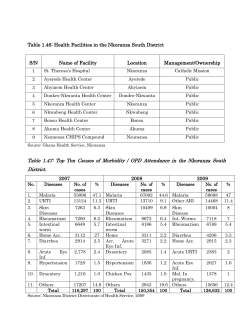


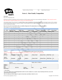


© Copyright 2026