
NLGA based Active Control in Aerospace
Alma Mater Studiorum – Università di Bologna
DOTTORATO DI RICERCA IN
Automatica e Ricerca Operativa
Ciclo XXVII
Settore Concorsuale di afferenza: 09/G1
Settore Scientifico disciplinare: ING-INF/04
NLGA based Active Control in Aerospace:
fault tolerability, disturbance rejection, and
parameter estimation
Presentata da: Nicola Mimmo
Coordinatore Dottorato
prof. Daniele VIGO
Relatore
prof. Lorenzo Marconi
Correlatore
prof. Paolo Castaldi
Esame finale anno 2015
". . . mais de toutes les sciences la plus absurde, à mon avis, et celle qui est la plus capable
d’étouffer toute espèce de génie, c’est la géométrie. Cette science ridicule a pour objet des
surfaces, des lignes, et des points, qui n’existent pas dans la nature. On fait passer en esprit
cent mille lignes courbes entre un cercle et une ligne droite qui le touche, quoique dans la réalité
on n’y puisse pas passer un fétu. La géométrie, en vérité, n’est qu’une mauvaise plaisanterie."
Voltaire
ALMA MATER STUDIORUM – UNIVERSITA’ DI BOLOGNA
Abstract
School of Engineering and Architecture
Department of Electrical, Electronic and Information Engineering
”Guglielmo Marconi”
Doctor of Philosophy
NLGA based Active Control in Aerospace: fault tolerability, disturbance rejection,
and parameter estimation
by Nicola Mimmo
A new control scheme has been presented in this thesis. Based on the NonLinear Geometric
Approach, the proposed Active Control System represents a new way to see the reconfigurable
controllers for aerospace applications. The presence of the Diagnosis module (providing the
estimation of generic signals which, based on the case, can be faults, disturbances or system
parameters), mean feature of the depicted Active Control System, is a characteristic shared by
three well known control systems: the Active Fault Tolerant Controls, the Indirect Adaptive
Controls and the Active Disturbance Rejection Controls. The standard NonLinear Geometric
Approach (NLGA) has been accurately investigated and than improved to extend its applicability
to more complex models. The standard NLGA procedure has been modified to take account
of feasible and estimable sets of unknown signals. Furthermore the application of the Singular
Perturbations approximation has led to the solution of Detection and Isolation problems in
scenarios too complex to be solved by the standard NLGA. Also the estimation process has
been improved, where multiple redundant measuremtent are available, by the introduction of
a new algorithm, here called “Least Squares - Sliding Mode”. It guarantees optimality, in the
sense of the least squares, and finite estimation time, in the sense of the sliding mode. The
Active Control System concept has been formalized in two controller: a nonlinear backstepping
controller and a nonlinear composite controller. Particularly interesting is the integration, in
the controller design, of the estimations coming from the Diagnosis module. Stability proofs are
provided for both the control schemes. Finally, different applications in aerospace have been
provided to show the applicability and the effectiveness of the proposed NLGA-based Active
Control System.
Acknowledgements
I would like to express deep gratitude to my academic advisor Prof. P. Castaldi for his consistent
encouragement, motivation and guidance throughout my study at University of Bologna. He has
provided me with unquenchable enthusiasm, vision, and wisdoms, which inspired me from the
beginning to the end. I also wish to thank Prof. L. Marconi for believing in me since the first
day of my doctorate.
I can’t forget my company tutors Dr. P. Goupil and Dr. R. Dayre for their great support,
availability and congeniality, background of my inestimable technical improvement during my
extraordinary six months in Toulouse.
I would also like to thank all my friends and colleagues at University of Bologna, particularly
Prof. M. Zanzi, Ing. A. Ghetti, Ing. F. Pieri, Dr. P. Baldi and Ing. C. Bezziccheri, with whom I
spent a lot of time both at work and in spare time. They made my years at university’s hangar
labs, in Forlì, enjoyable and memorable.
Last but by no means least, I am most sincerely grateful to my girlfriend, Ofelia, for her love
and support over the years. She has always been a pillar of strength, inspiration and support.
I could never thank my family for their unconditional love, without which I would never have
come so far.
iii
Contents
Acknowledgements
iii
Contents
iv
List of Figures
vi
Abbreviations
vii
Symbols
viii
1 Introduction and Motivations
1
1.1
Thesis contribution . . . . . . . . . . . . . . . . . . . . . . . . . . . . . . . . . . .
6
1.2
Thesis Outline . . . . . . . . . . . . . . . . . . . . . . . . . . . . . . . . . . . . .
8
2 NLGA based Active Control Scheme
2.1
NLGA based Detection and Diagnosis Module . . . . . . . . . . . . . . . . . . . .
13
2.1.1
NLGA based Detection and Isolation Technique . . . . . . . . . . . . . . .
14
2.1.1.1
The standard NLGA based Detection and Isolation Technique .
14
2.1.1.2
NLGA Applicability Improvement: Output to Input Mapping
Technique . . . . . . . . . . . . . . . . . . . . . . . . . . . . . . .
17
NLGA Applicability Improvement: the Singular Perturbation
Approximation . . . . . . . . . . . . . . . . . . . . . . . . . . . .
19
Formulations and Solutions of Detection and Isolation Problems
21
2.1.1.3
2.1.1.4
2.1.2
Detection Residuals . . . . . . . . . . . . . . . . . . . . . . . . . . . . . .
25
2.1.3
Isolation Logic . . . . . . . . . . . . . . . . . . . . . . . . . . . . . . . . .
28
2.1.4
Estimation Filters . . . . . . . . . . . . . . . . . . . . . . . . . . . . . . .
29
2.1.4.1
Least Squares with forgetting factor . . . . . . . . . . . . . . . .
30
2.1.4.2
Radial Basis Functions . . . . . . . . . . . . . . . . . . . . . . .
33
2.1.4.3
A new algorithm: Least Squares - Sliding Mode
. . . . . . . . .
34
NLGA based Detection and Diagnosis module: Summary . . . . . . . . .
37
Nominal Controller . . . . . . . . . . . . . . . . . . . . . . . . . . . . . . . . . . .
38
2.2.1
Backstepping Controller . . . . . . . . . . . . . . . . . . . . . . . . . . . .
39
2.2.1.1
39
2.1.5
2.2
9
Active Backstepping Controller Design Concept . . . . . . . . . .
iv
Contents
2.2.2
v
2.2.1.2
Stability analysis of the Active BackStepping Control . . . . . .
41
2.2.1.3
Stability of the Active Control . . . . . . . . . . . . . . . . . . .
43
Active Composite Controller . . . . . . . . . . . . . . . . . . . . . . . . . .
45
2.2.2.1
Generalized Faults Scenario . . . . . . . . . . . . . . . . . . . . .
46
2.2.2.2
Modeling the faulty plant . . . . . . . . . . . . . . . . . . . . . .
46
2.2.2.3
Control problem formulation and solution . . . . . . . . . . . . .
47
2.2.2.4
Feedback Linearization for the Reduced Errors Model . . . . . .
48
2.2.2.5
Feedback Linearization for the Boudary–Layer Error Model . . .
49
2.2.2.6
Stability analysis of the Active Fault Tolerant Composite Control 49
3 Case Studies
3.1
3.2
3.3
3.4
56
Aircraft . . . . . . . . . . . . . . . . . . . . . . . . . . . . . . . . . . . . . . . . .
58
3.1.1
Active Fault Tolerant Control - Case 1 . . . . . . . . . . . . . . . . . . . .
62
3.1.2
Active Fault Tolerant Control - Case 2 . . . . . . . . . . . . . . . . . . . .
64
3.1.3
Active Fault Tolerant Control - Case 3 . . . . . . . . . . . . . . . . . . . .
67
3.1.4
Active Wind Rejection Control . . . . . . . . . . . . . . . . . . . . . . . .
69
3.1.5
Flight Parameter Estimation for Extended Guidance Navigation and Control 74
Fixed Wing UAV . . . . . . . . . . . . . . . . . . . . . . . . . . . . . . . . . . . .
79
3.2.1
Active Fault Tolerant Control . . . . . . . . . . . . . . . . . . . . . . . . .
80
Satellite . . . . . . . . . . . . . . . . . . . . . . . . . . . . . . . . . . . . . . . . .
82
3.3.1
Active Fault Tolerant Control . . . . . . . . . . . . . . . . . . . . . . . . .
83
Quad Rotor . . . . . . . . . . . . . . . . . . . . . . . . . . . . . . . . . . . . . . .
86
3.4.1
89
Active Disturbance Rejection Control
. . . . . . . . . . . . . . . . . . . .
4 Conclusions
92
Bibliography
93
List of Figures
2.1
2.2
Active Control Scheme . . . . . . . . . . . . . . . . . . . . . . . . . . . . . . . . .
NLGA based Detection and Diagnosis Module . . . . . . . . . . . . . . . . . . . .
10
13
3.1
3.2
3.3
3.4
3.5
3.6
3.7
Aicraft simulator structure. . . . . . . . . . . . . . . . . . . . . . . . . . . . . . .
Estimate fˆδe of fδe fault. . . . . . . . . . . . . . . . . . . . . . . . . . . . . . . . .
Estimate fˆδth of fδth fault. . . . . . . . . . . . . . . . . . . . . . . . . . . . . . . .
Aircraft state with and without AFTC scheme: case of fault on δe . . . . . . . . .
Aircraft state with and without AFTC scheme: case of fault on δth . . . . . . . . .
Estimation of sinusoidal concurrent faults on δth and δe . . . . . . . . . . . . . . .
Aircraft state with and without AFTC scheme: case of concurrent faults on δth
and δe . . . . . . . . . . . . . . . . . . . . . . . . . . . . . . . . . . . . . . . . . . .
Distance from the glide slope with and without AFTC scheme: case of concurrent
faults on δth and δe . . . . . . . . . . . . . . . . . . . . . . . . . . . . . . . . . . .
Detection residuals behavior: comparison for isolation. . . . . . . . . . . . . . . .
Fault Estimation: FˆV estimates FV . . . . . . . . . . . . . . . . . . . . . . . . . .
State error, e = [e1 , e2 ]T : the designed AFTC, when engaged, guarantees faultless–
like performance. . . . . . . . . . . . . . . . . . . . . . . . . . . . . . . . . . . . .
Comparison of the simulated and estimated horizontal wind component. . . . . .
Comparison of the simulated and estimated vertical wind component. . . . . . . .
Comparison of the simulated and estimated rotational wind component. . . . . .
Comparison of the simulated and estimated horizontal wind derivative. . . . . . .
Comparison of the simulated and estimated vertical wind derivative. . . . . . . .
Aircraft trajectory in the case of the controller with and without wind compensation.
State evolutions in the case of the controller with and without wind compensation.
Surface – actuator: j-th system . . . . . . . . . . . . . . . . . . . . . . . . . . . .
Airspeed Virtual Sensor: performance . . . . . . . . . . . . . . . . . . . . . . . .
Recursive Detection and Isolation Scheme based on Estimation . . . . . . . . . .
FW-UAV: Estimation and tracking performance . . . . . . . . . . . . . . . . . . .
Satellite simulator scheme . . . . . . . . . . . . . . . . . . . . . . . . . . . . . . .
Satellite: Estimation and tracking performance - case of step faults . . . . . . . .
Satellite: Estimation and tracking performance - case of ramp faults . . . . . . .
Satellite: Estimation and tracking performance - case of sinusoidal faults . . . . .
Quadrotor simulator scheme . . . . . . . . . . . . . . . . . . . . . . . . . . . . . .
Exogenous disturbance and its estimation. . . . . . . . . . . . . . . . . . . . . . .
Inertial position in the case of the controller with and without disturbances compensation. . . . . . . . . . . . . . . . . . . . . . . . . . . . . . . . . . . . . . . . .
Inertial speed in the case of the controller with and without disturbances compensation. . . . . . . . . . . . . . . . . . . . . . . . . . . . . . . . . . . . . . . . .
59
63
64
64
65
66
3.8
3.9
3.10
3.11
3.12
3.13
3.14
3.15
3.16
3.17
3.18
3.19
3.20
3.21
3.22
3.23
3.24
3.25
3.26
3.27
3.28
3.29
3.30
vi
66
67
68
69
70
71
71
72
72
73
73
74
76
78
81
81
83
84
85
85
87
88
89
90
Abbreviations
ADRC
Active Disturbance Rejection Control
AFTC
Active Fault Tolerant Control
BS
BackStepping
CAS
Calibrated Air Speed
DD
Detection and Diagnosis
DI
Detection and Isolation
FL
Feedback Linearization
LS
Least Squares
LES
Locally Exponentially Stable
NED
North-East-Down local inertial axes
NLGA
NonLinear Geometric Approach
RBF-NN
Rarial Basis Functions Neural Network
RPM
Revolution Per Minutes
RM
Residual Matrix
SM
Sliding Mode
SP
Singular Perturbations
TAS
True Air Speed
UAV
Unmanned Aerial Vehicle
o.c.a.
observability codistribution algorithm
vii
Symbols
x
state vector
¯1
x
state vector of the first subsystem provided by the NLGA
¯2
x
state vector of the second subsystem provided by the NLGA
¯3
x
state vector of the third subsystem provided by the NLGA
y
output vector
¯1
y
output vector of the first subsystem provided by the NLGA
¯2
y
output vector of the second subsystem provided by the NLGA
u
input vector
f
unknown signals vector
fu
input faults vector
fsys
disturbance and system faults vector
fy
output faults vector
fs
set of undesired signals to be diagnosed
ds
generalized disturbance to be decoupled
h (x)
output map
n (x)
vector field
g (x)
input vector field
l (x)
fs vector field
p (x)
ds vector field
ˆ
(·)
estimation of (·)
X
compact set in the state space
Y
compact set in the output space
U
compact set in the input space
viii
Symbols
ix
Fu
compact set in the input faults space
Fy
compact set in the output faults space
Fsys
compact set in the disturbances and system faults space
Nr
number of minimal detection and isolation sets
Simin
i-th minimal detection and isolation set
R
residuals set
Ω
residual subset
r
analog residuals vector
rd
digital residuals vector
Jr
residual evaluation function
Jth
residual evaluation function threshold
`n
state space dimension
`m
output space dimension
`u
input space dimension
`sys
disturbances and system faults space dimension
`f
dimension of f
νs
dimension of fs
ΣP∗
minimal conditioned invariant distribution containing P
P
distribution spanned by the columns of ps
(ΣP∗ )⊥
codistribution orthogonal to ΣP∗
Ω∗
maximal observability codistribution contained in (ΣP∗ )⊥
ξ
vector of estimation activation signals
ε
singular perturbation parameter
m
rigid body mass
VI,B
inertial speed expressed in body axes
ΩB
rotational speed in body axes
FB
external forces expressed in body axes
I
rigid body inertia matrix
Symbols
x
MB
external torques expressed in body axes
PI
inertial rigid body position
RB→I
rotation matrix from body to inertial axes
S (·)
skew-symmetric matrix
ρ
air density
S
reference area
Va
True AirSpeed
M
Mach number
c¯
aerodynamic mean chord
Cx
x-body aerodynamic force coefficient
Cy
y-body aerodynamic force coefficient
Cz
z-body aerodynamic force coefficient
CD
x-wind aerodynamic force coefficient
CY
y-wind aerodynamic force coefficient
CL
z-wind aerodynamic force coefficient
Cl
x-body aerodynamic momentum coefficient
Cm
y-body aerodynamic momentum coefficient
Cn
z-body aerodynamic momentum coefficient
To my parents
for their unwavering love
xi
Chapter 1
Introduction and Motivations
T
he unknown and unmeasurable variations of the process parameters or exogenous
unknown signals can degrade the performances of the control systems. Feedback
is basically used in conventional control systems to reject the effect of disturbances
or model uncertainties upon the controlled variables and to bring them back to
their desired values according to the requirements. To achieve this, the controlled variables are
measured, then the measurements are compared with the desired values and the difference is fed
into the controller which generates the appropriate control. Modern technological systems rely
on sophisticated robust controls to meet increased performance requirements. For such systems,
the required robustness can be achieved via advanced control systems, which can be broadly
classified into active and passive.
A Passive Control System can tolerate a predefined set of exogenous unknown signals (such as
disturbances, faults, . . . ) or model mismatching (parameters uncertainties) while accomplishing
its mission satisfactory without the need for control reconfiguration.
An Active Control System, on the other hand, relies on a Diagnosis process to estimate
uncertain model parameters or exogenous unknown functions affecting the system’s performance.
Accordingly, the control law is reconfigured on-line.
In the presence of variations of the dynamic characteristics of a plant to be controlled, passive
robust control design of the conventional feedback control system is a powerful tool for achieving
a satisfactory level of performance for a family of plant models. This family is often defined by
means of a nominal model and a size of the uncertainties. The range of uncertainty domain for
which satisfactory performances can be achieved depends upon the problem. Sometimes, a large
domain of uncertainty can be tolerated, while in other cases, the uncertainty tolerance range
may be very small. If the desired performances cannot be achieved for the full range of possible
parameter variations, active control has to be considered in addition to a passive robust control
1
Chapter 1. Introduction and Motivations
2
design. Furthermore, the tuning of a passive robust design for the true nominal model using an
active control technique will improve the achieved performance of the passive robust controller
design. Therefore, robust control design will benefit from the use of active control in terms of
performance improvements and extension of the range of operation.
This work groups under the same root several Active Control techniques whose main three
representatives are:
Active Fault Tolerant Controls. An Active Fault Tolerant Control System (AFTCS) represents a strategy for increasing plant reliability and availability and for reducing the risk
of safety hazard [1]. An AFTCS is designed to continue operations, with graceful degradation in performance, by accommodating faults in early stage of their development, such
that minor fault in a subsystem do not develop in a failure at system level [2]. A fault
is defined as an unpermitted deviation of at least one characteristic property
or parameter of the system from the acceptable behavior. Faults may take
place in any system component (actuators, sensors, plant components, or any
combination) [3]. The fault is a state that may lead to a malfunction or a failure in the
system. The main task of AFTCS is on-line reconfiguration of the controller. For this to
be possible, detailed information about fault-induced changes is required. In this context,
a fault Detection and Diagnosis module plays a crucial role in AFTCS: it monitors system
performance, detect the occurrence of faults, and to determine their magnitude, indeed.
Indirect Adaptive Controls. An Adaptive Controller changes itself so that its behavior will
conform to new or changed circumstances. The words “adaptive systems” and “adaptive
control” have been used as early as 1950 [4]. The design of autopilots for high-performance
aircraft was one of the primary motivations for active research on adaptive control in the
early 1950s. Aircraft operate over a wide range of speeds and altitudes, and their dynamics
are nonlinear and conceptually time varying. As aircraft go through different flight conditions, the operating point changes and the output response y(t) carries information about
the state x as well as the parameters. In principle, a sophisticated feedback controller
should be able to learn about parameter changes by processing y(t) and use the appropriate gains to accommodate them. This argument led to a feedback control structure on
which adaptive control is based, see [5]. An Adaptive Controller is formed by combining
an on-line parameter estimator (Diagnosis module), which provides estimates of unknown
parameters at each instant, with a control law that is motivated from the known parameter case. In Indirect Adaptive Control, the plant parameters are estimated on-line by the
Diagnosis module and used to calculate the controller parameters. This approach has also
been referred to as explicit adaptive control, because the design is based on an explicit
plant model. The basic idea is that a suitable controller can be designed on-line if a model
of the plant is estimated on-line, by an appropriate Diagnosis module, from the available
Chapter 1. Introduction and Motivations
3
input-output measurements. The scheme is termed indirect because the adaptation of the
controller parameters is done in two stages: on-line estimation of the plant parameters
and on-line computation of the controller parameters based on the current estimated plant
model.
Active Disturbance Rejection Controls. Active Disturbance Rejection Control (ADRC) is
Han’s way out of the robust control paradox [6]. The term was first used in [7] where his
unique ideas were first systematically introduced into the English literature. The central
idea of Active Disturbance Rejection is recalled in [8]: the control of a complex nonlinear,
time-varying, and uncertain process is reduced to a simple problem by a direct and active
estimation, by a Diagnosis module, and rejection (cancellation) of the generalized disturbance, interpreted as the vector field representing all the model uncertainties affecting the
system dynamics. Anyway, information about physical disturbance acting on the systems
can be very useful for performance evaluation, so, in this thesis, the model uncertainties
to be estimated, by the Diagnosis module, and rejected are represented by exogenous unknown signals, such as non-manipulable inputs, rather than their effects on the system
dynamics.
The above mentioned active control techniques share a common feature: the presence the Diagnosis module. Literature presents plenty of techniques for the Diagnosis process and, in
general, these approaches can be categorized into signal-based and model based technique [9].
Signal-based methods detect the occurrence of undesired signals by testing specific properties
of measurements. In a model-based method, the Diagnosis module is, in the most general abstraction, composed by two parts: the Detection and Isolation block and the Estimation unit.
In turn, the Detection and Isolation module can be formally divided in two subsystems: the
Detection system, which provides a set of residuals indicating the occurrence of a certain signal,
and an Isolation logic, that elaborates these residuals to indicate the location of this signal into
the system. Usually, the analog detection residuals are converted to digital by comparing the
residual with a possibly adaptive threshold [10], [11], [12], [13]. Depending on the case, the
Detection module can be indispensable, when information about the occurrence of a signal is
needed despite the presence of other unknowns, or not necessarily present, when information
about the occurrence of a signal is not required. The existence of a Detection system implies
the presence of a set of residuals and consequently, of an Isolation logic, that can be, depending
on the structure of the residuals, as complicated as required or so obvious to be neglected. As
example, let’s image the possibility to have a set of “dedicated” residuals (each residual in this
set is dedicated to only and only one signal among the set of unknown signals to be estimated, in
a one-to-one correspondence). In this case the isolation logic can be represented by an “identity”
matrix, so, it exists but is straightforward. Usually the Estimation unit is switched on, after the
occurrence of the signal has been detected and the location of the signal has been determined,
Chapter 1. Introduction and Motivations
4
by an activation signal coming from the Detection and Isolation module. In the special case
of dedicated residuals set the estimation can always be kept active if there is the need of a
continuous estimation.
Two major approaches have been used in model-based detection residual generation: qualitative
(heuristic) methods and quantitative (analytic) methods [11], [14]. To design an Active Control,
precise knowledge about the plant dynamics need to be known after the occurrence of a undesired
signals corrupting the nominal system behavior. Hence, more emphasis has been placed upon
quantitative model-based diagnosis approaches.
Three main classes of analytical model-based residual generators exist: observer-based approaches, parity relations approaches and parameter estimation (or system identification) approaches. The principle of observer-based approaches is to estimate the system variables with
an observer (Luenberger, Kalman, . . . ) and to use the estimation errors/innovations as residuals
[12], [15], [16], [17], [18], [19]. In the parity relations approaches, the residuals are computed as
difference between the measured outputs and the estimated outputs and their associated derivatives. The method reshapes the primary residual signals using a transformation matrix to make
the residual insensitive to unknown disturbances and to increase signal estimation performances.
The parity relations approach has been developed in time domain [20] and in frequency domain
[21]. The parameter estimation methods, for Detection and Isolation, are particularly suitable
for systems where the undesired signals correspond to an undesired behavior of physical coefficients of the process. By continuously estimating the parameters of a process model, residuals
are computed as the parameter estimation errors. To successfully isolate the undesired signal,
the mapping from the model coefficients to the process parameters must exist and be known.
Different algorithms for parameter estimation have been proposed: least square estimation, instrumental variable approach, output error methods [22], sliding mode estimation [23], neural
network estimation [24], and extended Kalman filters [25].
Furthermore, several interesting approaches have been utilized to design and implement Detection and Isolation algorithms such as the Geometric Approach for both linear and non linear
cases.
Starting from the theoretical seminal works [26] and [27], the Linear Geometric Approach has
been investigated in [28] and [29], whereas several interesting applications can be found in [30] for
periodic systems and in [31] and [32] for systems whose dynamics has a Markovian description.
Linear systems with time delays have been investigate in [33], [34] and [35], and further particular
applications can be found about Fornasini-Marchesini 2D Systems [36], discrete time systems
[37] and systems with time varying perturbations [38].
On the road toward nonlinear systems, [39] presented remarkable aspects on bilinear systems.
Chapter 1. Introduction and Motivations
5
The NonLinear Geometric Approach came as natural development of its linear counterpart. The
first theoretical works is [40], further developed in [41] and [42], and investigated in [43] and [44].
Interesting applications of the NLGA can be found in [45] for hybrid systems, in [46] and [47] for
parabolic and hyperbolic partial differential equations, in [48] for robotic applications, in [49] for
industrial applications. A tutorial on the NLGA has been provided in [50]. Finally, lots of NLGA
aerospace applications for fault detection and isolation have been published: [51] on a Vertical
Take Off and Landing aircraft, [52] on a network of UAV, [53], [54], [55], [56], [57], [58] and [59]
on aircraft and [60], [61] and [62] for satellites. The NLGA applicability, typically committed
to detect and isolate faults, has be extended for the isolation and the successive estimation of
external disturbances. Interesting works are [63] and [64] for aircraft applications and [65] in the
case of quadrotors.
In this thesis, the NLGA constitutes the base for the design of Active Controls in aerospace.
Model-based Detection and Isolation techniques makes use of mathematical model of the system.
However, a perfectly accurate mathematical model of a physical system is never available. Hence,
there is always a mismatch between the actual process and its mathematical model. The effects
of modeling uncertainties, disturbances and noise are therefore the most crucial point in the
model-based Detection and Isolation concept and the solution of this problem is the key for its
practical applicability [3]. To overcome this problems, a model-based Detection and Isolation
scheme has to be insensitive to model uncertainties. Sometimes, a simple reduction of the
sensitivity to model uncertainties does not solve the problem: the sensitivity reduction may be
also associated to a reduction of the sensitivity to the signals to be detected and isolated [3],
indeed. In this thesis, in order to accommodate the application of the Detection and Isolation
concepts, disturbances and parameter uncertainties of the monitored plans, as well as faults are
modeled in the form of unknown input signals. The application of the NLGA, provided certain
conditions are satisfied, allows the generation of residuals that are perfectly (analytically) decoupled from the sources of uncertainty but not trivially dependent on the unknown signal to
be detected and isolated.
Chapter 1. Introduction and Motivations
1.1
6
Thesis contribution
This work presents an Active Control scheme, for aerospace applications, whose main features
are the Diagnosis module and its design technique, i.e. the NonLinear Geometric Approach.
The main contributions of this thesis are:
• Control systems unification: the Active Fault Tolerant Controls, the Indirect Adaptive
Controls and the Active Disturbance Rejection Controls can be regarded as members of
the same family of controllers, characterized by the presence of a Diagnosis module. This
thesis proposes a more general concept of Active Control that, based on the definition of
the unknown undesired signals acting on the plant, covers all these three methodologies,
see Section 2;
• Standard NLGA applicability improvement: the application of the Singular Perturbations approximation allows, with a weaker decoupling property, the solution of the
problem of Detection and Isolation where multiple non concurrent faults are affecting both
the inputs and the outputs, see Section 2.1.1.3;
• Standard NLGA procedure improvement: the standard NLGA proposed by [40] and
improved by [41] can be further extended by modifying the algorithm proposed in [41].
This work suggests two algorithm modifications to take account of feasible and estimable
sets of unknown signals, see Section 2.1.1.4;
• A new estimation algorithm: the Detection and Isolation robustness is important
as well as the estimation accuracy. In the context of multiple redundant measurements,
this works proposes a knew estimation algorithm that represents a fusion between two
well known techniques, i.e. the Least Squares (LS) and the Sliding Modes (SM), that
guarantees optimality, in the sense of the least squares, and finite estimation time, in the
sense of the sliding mode. See Section 2.1.4.3;
• Design, with stability proofs, of two Active Control Systems for aerospace
applications: a complete design of a nonlinear backstepping controller and a nonlinear
composite controller is shown in Section 2.2. For these two controllers a proper Diagnosis module is associated and the stability proof for the overall Active Control System is
provided. The controllers structure, based on the elementary brick of the Feedback Linearisation, is particularly suitable to exploit the estimations coming from the Diagnosis
module;
• Aerospace applications: the methodology developed in this this work has been applied
to typical aerospace systems such as aircraft, spacecraft, fixed wind UAVs and quadrotors.
The results in Section 3 are encouraging and show the applicability effectiveness of the
Chapter 1. Introduction and Motivations
7
NLGA-based methodology, able to cover different applications in aerospace. The application of the improved NLGA to these aerospace systems has led to the design of new
controllers and new Diagnosis schemes able to solve, for the first time, complex problems
such as the detection and the isolation of multiple faults of all actuators and sensors.
Chapter 1. Introduction and Motivations
1.2
8
Thesis Outline
This work is organized in two main Sections: Section 2 describes all the methodological aspects related to the proposed NLGA-based Active Control System, whereas Section 3 shows the
application of the hereafter mentioned methodology to aerospace cases.
In particular, Section 2 is divided to detail, step by step, all the components of the NLGA-based
Active Control System: Section 2.1.1 recalls the standard NLGA and presents some methodological advances, Section 2.1.2 depicts how to design robust Detection residual sets, Section
2.1.3 presents the residual matrix concept at the base of the Isolation technique, Section 2.1.4
details three kind of estimation algorithms and, finally, Section 2.2 shows, with stability proofs,
how to integrate, in the controller design, the estimation coming from the Diagnosis module.
Section 3 is dedicated to the application of the NLGA-based Active Control System. After a
brief introduction highlighting the model commonalities of all the proposed aerospace plants (see
Section 3), five different scenarios of faults, disturbances and flight parameters are considered
for aircraft in Section 3.1 whereas Sections from 3.2 to 3.4 cover the remaining plants that are
a fixed wing UAV, a spacecraft and a quadrotor.
Final remarks and conclusions are presented in Section 4.
Chapter 2
NLGA based Active Control Scheme
T
he Active Control schemes considered in this thesis are composed by two main parts:
the Nominal Controller and the Estimation Module. These two modules work
together to achieve the output tracking, that is the control goal, i.e. to make
y(t) following the reference time function, yREF (t), despite the presence of faults,
uncertainties and disturbances. Generically speaking, the control loop can be affected by three
kind of disturbances:
• unknown functions affecting the input, fu ;
• unknown functions affecting the plant dynamics, fsys ;
• unknown functions affecting the output, fy .
Figure 2.1 schematically depicts the control problem and the unknown functions scenario: the
plant is forced by the controller actions u, linearly corrupted by the unknown fu , while the
dynamics of the plant is influenced by the unknown functions fsys . The state x is measured by
y, through h (x) which is affected by the unknown functions fy . Finally, the nominal controller
receives the estimation ˆfs of some of (at most all of) the unknown functions.
The scheme presented in Figure 2.1 is mathematically described by the following Multi Input –
Multi Output (MIMO) system:
(
x˙ = n(x) + g(x) [u (t) + fu (x, t)] + l(x) fsys (x, t)
y = h(x) + fy (x, t)
(2.1)
where x ∈ X ⊂ R`n , y ∈ Y ⊂ R`m , u ∈ U ⊂ R`u , fu ∈ Fu ⊂ U, fy ∈ Fy ⊂ Y, fsys ∈ Fsys ⊂ R`sys
and n(x), the columns of g(x) and l(x) are smooth vector fields, and h(x) is a smooth map.
9
Chapter 2. NLGA based Active Control Scheme
10
Figure 2.1: Active Control Scheme
Finally fs ⊆ f = {fu ∪ fsys ∪ fy }, fs ∈ Rνs with νs ≤ `f = `u + `sys + `y , represents the set of
unknown functions estimated by ˆfs .
As stated in Section 1, Active Control Systems strictly rely on a Diagnosis process to estimate
uncertain model parameters or exogenous unknown functions affecting the system’s performance.
Then, since the Diagnosis module assumes a great relevance for this kind of control schemes
it’s worth understand its mean features. The estimation module can be characterized by the
presence of a detection logic which activate the estimation process only in the case where the
fault is detected affecting the system. This simple, but important, aspect allows to avoid the
continuous noisy feedback, which is typical of adaptive control schemes. Generally speaking, the
estimations are obtained by means of the following three steps:
1. Detection: this initial stage tips off, and indicates by a binary signal, the presence of the
unknown functions (e.g. is the system affected by a fault or not?);
2. Isolation: the second phase identifies, usually by a boolean logics, the location of unknown
functions (where the unknown function is affecting the system);
3. Estimation: the final step provides the estimation of the detected and isolated unknown
function.
The Active Control scheme presented in this work, can assume the features proper of the adaptive
controls: as detailed in Section 2.1.1.1, the definition of fs , and its isolation properties can avoid
the need of an isolation logic, indeed. In this scenario, the three phases of Detection – Isolation
– Estimation are collapsed into one stage, continuously providing unknown functions estimation.
Chapter 2. NLGA based Active Control Scheme
11
Before entering in the detail of the NLGA, it is necessary to introduce the concept of the
generalized disturbance. As mentioned in this Section, this work deals with generic unknown
functions which can be interpreted as:
• fu (x, t) faults affecting the actuators;
• fy (x, t) faults corrupting the sensors;
• fsys (x, t) faults, disturbances and unknown parameters directly influencing the plant dynamics.
Furthermore, the following classifications are important to get the generality of the proposed
solution. The first division is based on the cardinality of fs :
• cardinality of fs = 1: fs is a scalar, i.e. fs = f . In this scenario, fs is called “single”
unknown function;
• cardinality of fs > 1: fs is a vector. This scenario covers the so called “multiple” unknown
functions.
The second grouping is made, only for the multiple unknown functions scenarios, on the contemporaneity. The multiple unknown functions are said to be:
• non-concurrent if the system is affected by just one component of fs per time;
• concurrent when the system is corrupted by more than one component of fs at the same
time, i.e. simultaneously.
The Active Control scheme proposed in this work is quite general and, based on the definition
of the Detection and Diagnosis module, allows the representation of three different well known
families of control schemes:
• Active Fault Tolerant Controls: these control systems is based on the Detection and
Isolation module to provide a system’s health monitoring function too. In this context,
the control actively reacts by exploiting the fault estimation only after the faults (seen as
external unknown functions) are detected and isolated. A common aerospace fault scenario
is represented by multiple non-concurrent faults (both on actuators and sensors);
• Indirect Adaptive Controls: the indirect adaptive controls are control systems able
to adapt themselves thanks to the estimation of unknown, possibly time varying, plant
parameters. In this control schemes the estimation is always active (it isn’t switched on by
Chapter 2. NLGA based Active Control Scheme
12
any activation signal, and the detection-isolation-estimation functions are collapsed and
indivisible). The set of the unknown varying parameters can be seen as scenario of multiple
concurrent unknown functions.
• Active Disturbance Rejection Controls: this class of controls shares some features
with both the Active Fault Tolerant Controls and the Indirect Adaptive Controls. Active
Disturbance Rejection systems are based on the estimation of external disturbances (such
as faults) that are always present on the system (such as plant parameters). Also this
scenario is characterized by the presence of multiple concurrent unknown functions, but,
the presence of a Detection and Isolation module is not ruled out: image, as example,
an aircraft landing in turbulences and wind shear conditions. The goal is to feedback
only the estimation of the wind shear components that overcome a threshold determined
by the turbulences intensity. In this way the nominal controller is not fed by pure noisy
estimations.
Thanks to the active structure, the Nominal Controller reacts to unknown functions affecting
the system by properly exploiting the estimations coming from the Estimation Module. On
the other hand, the Estimation Module should provide correct estimations as necessary, but not
sufficient condition, to allow a good active reaction (the necessary conditions stay in the nominal
controller). In this context, the NonLinear Geometic Approach (NLGA) constitutes a suitable
tools for constructing robust estimations.
The next Section describes the basics of the NLGA and the improvements that can be introduced
in the case of aerospace systems.
Chapter 2. NLGA based Active Control Scheme
2.1
13
NLGA based Detection and Diagnosis Module
The Detection and Diagnosis Module, depicted in Figure (2.2), aims to provide the estimation
of the selected part of the unknown functions, i.e. fs , by using all the available information. In
particular, it can exploit the corrupted output y, the uncorrupted control law u and the plant
model. The Detection and Diagnosis module, designed be the NonLinear Geometric Approach,
represents a solution of the following problem.
Problem 1. fs -DD Problem: Take the plant model 2.1 with the associated unknown functions
sets f and fs . Design, if possible, a Detection and Diagnosis module with inputs y and u, and
output ˆfs such that ˆfs asymptotically estimates the function fs , i.e. limt→∞ ˆfs = fs . Figure 2.2: NLGA based Detection and Diagnosis Module
Figure 2.2 contains two fluxes of information: the first one (dotted lines) represents the information associated to the knowledge of the mathematical model of the plant whereas the second
(continuous lines) indicates the information related to physical signals.
The NonLinear Geometric Approach, based on the knowledge of the plant model (model based
technique), provides new variables representing a subsystem of system (2.1) on which the estimation filters are designed. The estimation module contains a bank of νs estimation filters, each
of them switched-on by its relative activation signal, i.e. ξi , component of the activation vector
ξ. Finally, the activation vector ξ is the output of the Detection and Identification Module, also
based on the NLGA.
Chapter 2. NLGA based Active Control Scheme
2.1.1
14
NLGA based Detection and Isolation Technique
The first part of this Section details the standard NonLinear Geometric Approach whereas the
second and third parts respectively show how to extend the applicability of the standard NLGA
to more interesting scenarios and how to exploit the aerospace model common features to solve
real case problems.
2.1.1.1
The standard NLGA based Detection and Isolation Technique
This subsection recalls the standard NLGA, which was formally developed in [40] and generalized
by [41], on which both the detection residuals and the estimators design methodology are based.
The NLGA procedure for the solution of Detection and Isolation problem starts by defining two
quantities:
• the subsets fs = {f1 , ..., fνs } ⊆ f ;
• the complementary subset ds = f \ fs
The subset fs contains all the unknown functions that have to be estimated and, based on the
definition of “faults” in Section 1, it can be seen as a set of generalized faults, whereas ds , here
called generalized disturbances, collects all the remaining unknown functions from which the
residual rs has to be analytically decoupled, as described below.
This method relies on coordinate changes in the state and output spaces thus allowing to determine new descriptive variables, allowing to determine a sub-system affected only by fs . In
other words, the method provides one observable subsystem which, if it exists, is only affected
by fs , but unaffected by the other components of f to be decoupled, i.e. ds . For a comprehensive detailed application of the NLGA, referee to [50]. More precisely, the approach consider a
nonlinear system model in the form:
(
x˙ = g0 (x) +
y = h(x)
P`u
i=1 gi (x) ui
+ ls (x) fs + ps (x) ds
(2.2)
in which x ∈ X ⊂ R`n is the state vector, u(t) ∈ R`u is the control input vector, fs (t) ∈ R`s
is the s-th unknown function set to be estimated, ds (t) ∈ R`d =n−`s the generalized disturbance
vector embedding the remaining unknown function sets to be decoupled, y ∈ R`m the output
vector, n(x), gi (x) for 1 ≤ i ≤ `u , ls (x) = {l1 , ..., lνs } and the columns of ps (x) are smooth
vector fields, and h(x) is a smooth map. Equation (2.2) implicitly contains the assumption that
y = h(x), i.e. that fy = 0.
Chapter 2. NLGA based Active Control Scheme
15
Therefore, if P represents the distribution spanned by the column of ps (x), the design of the
strategy for the isolation of the generalized faults set fs with de–coupling from the generalized
disturbance ds , by means of the considered NLGA [40], is organised as follows:
• computation of ΣP∗ , i.e. the minimal conditioned invariant distribution containing P
(where P is the distribution spanned by the columns of ps (x));
• computation of Ω∗ , i.e. the maximal observability codistribution contained in (ΣP∗ )⊥ ;
• if lk (x) ∈
/ (Ω∗ )⊥ ∀ k ∈ {1, ..., νs }, fs –detectability condition, the generalized faults set is
detectable and a suitable change of coordinate can be determined.
The minimal conditioned invariant distribution ΣP∗ can be computed by means of the following
recursive algorithm:
(
S0
Sk+1
= P¯
Pu ¯
= S¯k + `i=0
gi , Sk ∩ ker {dh}
(2.3)
where `u is the number of inputs, S¯ represents the involutive closure of S, [g, ∆] is the distribution
spanned by all vector fields [g, τ ], with τ ∈ ∆, and [g, τ ] the Lie bracket of g, τ .
It can be shown that if there exists a k ≥ 0 such that Sk+1 = Sk , the algorithm (2.3) stops and
ΣP∗ = Sk [40].
Once ΣP∗ has been determined, Ω∗ can be obtained by exploiting the following algorithm:
(
Q0
Qk+1
= (ΣP∗ )⊥ ∩ span {dh}
Pu
[Lgi Qk + span {dh}]
= (ΣP∗ )⊥ ∩ `i=0
(2.4)
where Lg Γ denotes the codistribution spanned by all covector fields Lg ω, with ω ∈ Γ, and Lg ω
the derivative of ω along g.
If there exists an integer k ∗ such that Qk∗ = Qk∗ +1 , Qk∗ is indicated as o.c.a. (ΣP∗ )⊥ , where
the acronym o.c.a. stands for observability codistribution algorithm.
It can be shown that Qk∗ = o.c.a. (ΣP∗ )⊥ represents the maximal observability codistribution
contained in P ⊥ , i.e. Ω∗ [40]. Therefore, with reference to the model (2.2), when lk (x) ∈
/ (Ω∗ )⊥
∀ k ∈ {1, ..., νs }, the generalized disturbance ds can be decoupled and the generalized faults set
fs is detectable.
All the conditions above depicted are only “necessary” and nothing can be said about the possibility to create a residual if the following “sufficient” conditions are not verified.
As mentioned above, the application of the NLGA for solving the generalized faults set diagnosis
problem, described in [40], is based on a coordinate change in the state space and in the output
Chapter 2. NLGA based Active Control Scheme
16
space, Φ(x) and Ψ(y), respectively. They consist in a surjection Ψ1 and a function Φ1 such that
Ω∗ ∩ span {dh} = span {d (Ψ1 ◦ h)} and Ω∗ = span {dΦ1 }, where:
¯1
x
Φ(x) =
¯2
x
¯3
x
¯1
y
Ψ(y) =
¯2
y
Φ1 (x)
= H2 h(x)
Φ3 (x)
!
=
Ψ1 (y)
(2.5)
!
H2 y
are (local) diffeomorphisms, whilst H2 is a selection matrix, i.e. its rows are a subset of the rows
of the identity matrix. If the coordinate changes in (2.5) can be found, the “sufficient” conditions
¯ ), the system (2.2)
are verified and, by using the new (local) state and output coordinates (¯
x, y
is transformed as follows:
¯˙ 1
x
¯˙ 2
x
¯˙ 3
x
¯1
y
¯2
y
¯ 2 ) + g1 (¯
¯ 2 ) u + ls1 (¯
= n1 (¯
x1 , x
x1 , x
x) fs
= n2 (¯
x) + g2 (¯
x) u + ls2 (¯
x) fs + ps2 (¯
x) ds
= n3 (¯
x) + g3 (¯
x) u + ls3 (¯
x) fs + ps3 (¯
x ) ds
(2.6)
= h1 (¯
x1 )
¯2
= x
¯ 1 in Equation (2.6) is
with ls1 (¯
x) not identically zero. As described in [40], the subsystem x
¯ 3 is not directly available for measurements. In particular, the
locally weakly observable and x
¯ 3 -subsystem, is not present if the whole state x is measurable.
third subsystem, i.e. the x
This transformation can be applied to the system (2.2) if and only if the fs –detectability condition is satisfied. The system (2.2), in the new reference frame, can be decomposed into three
¯ 1 –subsystem) is always de–coupled from the
subsystems (2.6) where the first one (the so–called x
disturbance vector ds and affected by the generalized faults set fs as follows:
(
¯˙ 1 = n1 (¯
¯ 2 ) + g1 (¯
¯ 2 ) u + ls1 (¯
¯2, x
¯ 3 ) fs
x
x1 , y
x1 , y
x1 , y
¯1
y
= h1 (¯
x1 )
(2.7)
¯ 2 in (2.6) is assumed to be measured, the variable x
¯ 2 in (2.7) is considwhere, as the state x
¯ 2 . Even if the state x
¯ 3 isn’t available for direct
ered as independent input and denoted with y
measurements, the detection of fs is always guaranteed by observing that, since ls1 (¯
x) is not
identically zero, the presence of fs can be always find out by designing a filter for the detection
of ls1 fs .
Chapter 2. NLGA based Active Control Scheme
2.1.1.2
17
NLGA Applicability Improvement: Output to Input Mapping Technique
The methodology applicability can be extended by removing the hypothesis of the standard
NLGA, i.e. fy = 0 and assuming that the state x is directly available for measurement. In this
scenario, the plant dynamics is expressed by:
(
x˙ = n(x) + g(x) (u + fu ) + l(x) fsys
y = x + fy
(2.8)
Let’s rewrite the dynamics of (2.8) in terms of the output variables by introducing a simple
coordinate change T : R`n → R`n , z = y = x + fy :
(
z˙ = n(z − fy ) + g(z − fy ) (u + fu ) + l(z − fy ) fsys + f˙y
y = z
(2.9)
Even if the (2.9) has been obtained in a straightforward way, the resulting model is not affine
with respect to the faults and, as consequence, the NLGA can not be applicable. To overcome
this problem, [49] proposes a different coordinate change, from the state to the output variables,
which allows to write an unknown functions affine model, thus allowing the application of the
standard NLGA procedure.
The scenario of Equation (2.9), in terms of number of potentially concurrent unknown functions versus the number of available information (i.e. the number of states and outputs), is
really complex and generically not solvable with the standard NLGA. On the other hand, for
aerospace systems, taking into account fu and fy which represent faults and assuming that also
fsys represents only faults, it’s not wrong the assumption that the faults, even if multiple, are nonconcurrent (aerospace systems are such that the probability of multiple concurrent faults is very
low compared to the probability of multiple non-concurrent faults). The scenario, represented
by multiple non-concurrent faults, can not describe disturbances because they are concurrent
functions always affecting the system, despite the presence of faults.
The procedure proposed in [49] exploits the hypothesis of multiple but non-concurrent faults
to associate to the i-th component of fy , i.e. the physical output fault fyi , a number νi of
equivalent mathematical faults that are state dependent functions, generally without physical
interpretation and with a different time behavior respect to the physical fault fyi . Following
the procedure stated in [49] for modeling the sensor faults, it’s possible to introduce νi ≥ 1
always concurrent mathematical faults, fy∗i,k (k = 1, ..., νi ), in place of the physical fault fyi ∀i ∈
{1, ..., `n }. Whenever a physical sensor fault occurs, i.e. fyi 6= 0, all associated mathematical
faults fy∗i,k (i = 1, ..., νi ) will become nonzero.
Chapter 2. NLGA based Active Control Scheme
18
According to this modeling, in order to detect and isolate the single physical fault on the i-th
sensor, it will be sufficient to recognize the occurrence of any (one or more) of its associated
mathematical faults. To isolate a given set of faults from the remaining ones, as formalized in
[42], for the generic i-th sensor fault, [49] proposes the following modeling procedure:
1. Take the i-th element of x, i.e. xi , and look in the system model for all different (and, in
general, nonlinear) expressions φi,k (x, u), involving xi and such that the model is affine in
φi,k (x, u);
2. For each expression φi,k (x, u) found at the step 1, define the fault input fy∗i,k = φi,k (x, u) −
φi,k (x, u)|xi =yi , i.e., the error induced in the computation of φi,k (x, u) by the use of the
measured value yi in place of the real value xi , and compute the corresponding fault
vector field l∗i,k (x). Let us denote the number of faults introduced in this way by νi − 1.
Note that fy∗i,k is, by definition, only affected by a fault of the i-th state sensor (which is
consistent with the assumption of non-concurrency), and is zero whenever fy,i = 0, i.e.,
when xi = yi . As a result of this modeling step, any occurrence of the expression φi,k (x, u)
in the system model can be replaced by φi,k (x, u)|xi =yi + fy∗i,k , and the model is certainly
affine in the fault input fy∗i,k . Note that the right-hand side of Equation (2.8) will now be
only dependent on the variable yi and not on xi ;
3. Define the further fault input fy∗i,ν = x˙ i − y˙ i . The introduction of this additional fault input
i
in the model allows writing also the left-hand side of the i-th system equation in terms of
the new variable yi (with dynamics y˙ i = x˙ i − fy∗i,ν ). The fault vector field associated to
i
fy∗i,ν is, thus, l∗i,νi = −Ii ( Ii is the i-th column of the identity matrix);
i
4. If, for two indices j, k, we can write for l∗i,j = α(x)l∗i,k some real function α(x), then
∗ = f ∗ + α(x)f ∗ and eliminate f ∗ (vector field l∗ clearly remains the same).
set fi,k
i,j
i,j
i,k
i,k
With a slight abuse of notation, the symbol νi is still used to indicate the final number of
mathematical fault inputs corresponding to the i-th state sensor fault.
At this point, when the outputs are taken as new state variables for the system dynamics, the
general structure of Equation (2.2) is recovered. The final model, including the effect of all
(non-concurrent) faults of actuators and state sensors, is:
(
z˙
= g0 (z) +
y = z
P`u
i=1 gi (z) (ui
+ fui ) +
P`n Pνi
i=1
∗
∗
j=1 li,j (z) fyi,j
+
P`sys
i=1 li (z) fsysi
(2.10)
The set of the equivalent mathematical faults associated to the physical output fault fyi is indin
o
cated with fy∗i = fy∗i,j with j ∈ {1, ..., νi } whereas the set of all the the equivalent mathematical
faults associated to all the output physical faults fy is fy∗ = fy∗i with i ∈ {1, ..., `n }.
Chapter 2. NLGA based Active Control Scheme
19
The multiple non-concurrent fault scenario is represented by f = {fu ∪ fsys ∪ fy∗ } and contains
Pn
νi elements. The definition of the s-th elements, fs , is made by following this
`u + `sys + `i=1
scheme:
• for the i-th input fault fui , fs = fui and ls = gi ;
• for the i-th system fault fsysi , fs = fsysi and ls = li ;
h
i
• for the i-th output fault fyi , fs = fy∗i and ls = l∗yi , ..., l∗yiν .
1
i
where, the number of element of ls is defined as µs (that is equal to 1 for input and system faults
and νi for the output faults).
Introducing the additional assumption of non-concurrency of faults, results into much weaker
conditions for fs -DI than those given in [40]. In particular, the necessary and sufficient condition
for non-concurrent fs -DI (under full state availability and absence of disturbances) is, see [42]:
∀s, ∀j 6= s, ∃ k ∈ {1, ..., µs } : span{lsk } 6⊆ P¯j
OR
∃ h ∈ {1, ..., µj } : span{ljh } 6⊆ P¯s (2.11)
where P¯j = span{lj1 , ..., ljµj } and P¯j denotes the involutive closure of Pj , i.e., the closure of
under the Lie bracket operator. Finally, the elements of ls , the vector field associated to fs , are
indicated by ls1 , ..., lsµs . Note that, the two conditions in the left- and right-hand sides of the
“OR” operator in Equation (2.11) may not hold at the same time. Thus, it may happen that a
residual generator exists, that is affected by fs and not by fj , but that any residual affected by
fj is necessarily also affected by fs .
2.1.1.3
NLGA Applicability Improvement: the Singular Perturbation Approximation
Aerospace systems such as aircraft, UAV, quadrotors, satellites, ... show interesting common
plant features: their dynamics is describes with a six degrees of freedom model, indeed. Three of
these six degrees of freedom are relative to the rotational dynamics whereas the second group of
three degrees of freedom are representative of the translational dynamics. All of these aerospace
systems also show an inherent separation between rotational and translational dynamics where,
usually, the rotational dynamics is pretty faster than the translational one.
Chapter 2. NLGA based Active Control Scheme
20
Systems characterized by dynamics evolving on separated time scales are well represented, by
using the Singular Perturbation (SP) theory, as:
x˙ 1 = n1 (x1 , x2 , u, fu , fsys , ε)
εx˙ 2 = n2 (x1 , x2 , u, fu , fsys , ε)
y1 = x1 + fy1
(2.12)
y2 = x2 + fy2
where ε is the (small) perturbation parameter. As assumed in the previous Section, all the
unknown functions affecting the system are considered as non-concurrent faults.
In order to make clear the final benefit introduced by the Singular Perturbation approximation,
the Output to Input mapping procedure is firstly attempted without any approximation:
˜ 1 (z1 , z2 , fy∗1 , fy∗2 , u, fu , fsys , ε)
z˙ 1 = n
˜ 2 (z1 , z2 , fy∗1 , fy∗2 , u, fu , fsys , ε)
εz˙ 2 = n
y1 = z 1
(2.13)
y2 = z 2
Equation (2.13) shows that both the equivalent output faults fy∗1 and fy∗2 are influencing both
the dynamics of z1 and z2 .
Hypothesis 1. The Tikhonov’s theorem in [66] is valid even in presence of faults, i.e. it’s possible
to approximate the actual dynamics of the system (2.12) by it’s reduced and boundary layer
models.
Assuming that the Hypothesis 1 is verified then it’s possible to approximate the actual dynamics
of the aircraft (2.12) by its reduced and boundary layer models (ε = 0):
˜˙ 1 = n1 (˜
x
x1 , x2M , u, fu , fsys , 0)
0
η2 = φ2 (˜
x1 , η2 , u, fu , fsys , 0)
˜ 1 + fy1
y1 = x
(2.14)
y 2 = x 2 M + η 2 + f y2
where x2M = H (˜
x1 , u, fu , fsys ) is an isolated root x2 such that 0 = n2 (˜
x1 , x2 , u, fu , fsys , 0) and
0
η2 = x2 − x2M . The term η2 represents the derivative respect to the “fast” time scale τ , i.e.
0
η2 =
η2
dτ
=
η2
d(t/ε) .
Chapter 2. NLGA based Active Control Scheme
21
Following the same fault mapping procedure exploited in Section 2.1.1.2, it’s possible to rewrite
the approximated dynamics in terms of output variables:
˜˙ 1 = n
˜ 1 (˜
z
z1 , fy∗1 , u, fu , fsys , 0)
0
˜ 2 (˜
z2 = n
z1 , z2 , fy∗1 , fy∗2 , u, fu , fsys , 0)
y1 = z 1
(2.15)
y2 = z 2
Comparing the systems (2.13) and (2.15) it’s easy to see how, thanks to the application of the
SP, the equivalent mathematical output faults, fy∗2 are mapped only in the fast dynamics z2 thus
helping to meet the conditions required by the relaxed NLGA for non-concurrent fault isolation,
see Section 2.1.1.2.
Remark 1. Thanks to the Output to Input mapping procedure the systems (2.13) and (2.15) are
affine with respect to the unknown functions to be estimated.
The Detection and Isolation based on the singular perturbation approximation is valid only if
the Hypothesis 1 is verified, see [47]. In turn, this hypothesis relies on the stability of the approximated system that is strictly related to the implemented control law. In conclusion, in order
to make the singular perturbation detection and isolation technique valid, the controller have to
guarantee the stability of the system at any time: in absence of faults, during the detection, isolation and estimation transient and during the fault accommodation phase. Section 2.2.2 proposes
a stability analysis for an Active Fault Tolerant Control based on Singular Perturbations.
2.1.1.4
Formulations and Solutions of Detection and Isolation Problems
Problem 1 on the Detection and Diagnosis of the generalized faults set fs can be solved if all the
active components of fs can be estimated. This requirement is translated in the Detection and
Isolation of the active components of fs . So, one question arises: what is the maximum level
of information about the Detection and the Isolation of (sets of) generalized faults affecting the
system (2.2)?
The answer to this question has been provided in [41] and is based on the Set Detection and
Isolation procedure, in turn exploiting the NLGA detailed in 2.1.1.1. The solution has been
found by the introduction of the so-called “minimal” fsi –Detection ans Isolation sets (Simin ), i.e.
subsets of generalized faults, i.e. fsi ⊂ fs , such that:
• fsi is a Detection and Isolation set (fs –DI–set);
• fsi does not strictly include any other fs –DI–set.
Chapter 2. NLGA based Active Control Scheme
22
where an fs –DI–sets is defined as a subset fsi ⊂ fs such that is possible to find a residual rid
affected by each of the components in fsi and not affected by any other components in generalized
disturbance dsi = ds ∪ (fs \ fsi ).
min for system (2.2), a
For the computation of the list Slist of all minimal fs -DI-sets S1min , ..., SN
r
recursive algorithm, having the structure of a tree exploration, can be devised. The root of the
tree corresponds to the trivial fs -DI-set fs . The children of each node are all subsets obtained
by removing one element from the parent set. The exploration proceeds in depth as far as the
current set/node includes at least one generalized fault that can be isolated from its associated
generalized disturbance set. When this does not hold anymore, the algorithm steps back to the
parent node and explores the other children. When no child allows the prosecution of the search,
then the current node necessarily corresponds to a minimal fs -DI-set.
This thesis introduce a slight modification to the above mentioned algorithm by introducing
a new concept that lead to an “recursive” Detection and Isolation based on Estimation. The
concept is shown by the following didactic example where x = (x1 , x2 , x3 ):
x˙ 1 = n1 (x) + g1 (x)u + l11 (x)f1
x˙ 2 = n2 (x) + g2 (x)u + l21 (x)f1 + l22 (x)f2 + l23 (x)f3
x˙ 3 = n3 (x) + g3 (x)u + l31 (x)f1 + l32 (x)f2 + l33 (x)f3
(2.16)
y = x
The first minimal f -DI-set, S1min , can be intuitively found by observing system (2.16). The first
equation can be directly exploited to design a residual for the detection and the isolation of f1 ,
So, it is straightforward to define S1min = {f1 }. On the other hand, the possibility to create a
residual sensitive only to f2 (or f3 ) have to be checked by applying the NLGA procedure, as
example, by defining fs = {f2 } and ds = {f1 , f3 }. Even if the necessary conditions are satisfied,
this residual may not be found because the sufficiency conditions, listed in Section 2.1.1.1, may
not be verified thus leading to the impossibility of finding the needed coordinate change. So,
even if the procedure in [41] can find two new minimal sets S2min = {f2 } and S3min = {f3 }, if the
sufficient conditions are not verified, the second feasible minimal set is S2min = {f2 , f3 }. The
author introduces the concept of Detection and Isolation based on Estimation by observing that,
if f1 can be detected, isolated and also estimated, after the estimation convergence transient, f1
can be considered a known quantity. With this assumption the sufficiency may be verified by
eliminating the quantity f1 from the generalized disturbance ds . As example, for the isolation of
f2 , the NLGA procedure is now applied on fs = {f2 } and ds = {f3 }. At the end, the coordinate
change can be easier to be found. This new Detection and Isolation concept has been inserted
in the algorithm of [41] for the determination of the minimal feasible fsi –DI–sets Detection and
Isolation sets, and highlighted in bold.
Chapter 2. NLGA based Active Control Scheme
23
Minimal Feasible fs -DI-sets Algorithm
L = L0 = {l1 , ..., ls }
Slist = {0}
k=0
Flag = X %D&I based on Estimation (0 = OF F, 1 = ON )
[Slist , Nr ] = explore (L, Slist , k)
with
f unction [Slist , k] = explore (L, Slist , k)
kloc = k
P = span{ds , L0 \ L}
h
⊥ i⊥
if ∃ lσ ∈ L : span{lσ } 6⊆ o.c.a. ΣP∗
f or li ∈ L
[Slist , k] = explore (L \ li , Slist , k)
⊥ feastest = feasibiltiy o.c.a. ΣP
∗
if (k == kloc ).AND. (feastest == 1)
k =k+1
Skmin = {fj : lj ∈ L}
Slist = Slist , Skmin
is estimable).AND.(Flag == 1)
if (Smin
k
L0 = L0 \ Smin
k
L = L \ Smin
k
end
end
end
function [feastest ] = feasibiltiy (Ω∗ )
if sufficiency conditions in Section 2.1.1.1 are verified for Ω∗
feastest = 1
else
feastest = 0
end
d }, with r d designed to detect and isolate the f min –DI–set,
The set of residuals R = {r1d , ..., rN
si
i
r
provides all the available information about the detection and isolation of (sets of) generalized
faults in fs for the system (2.2). Finally, the “Minimal Feasible fs -DI-sets Algorithm” can be
exploited to solve classical fs -DI problems.
Chapter 2. NLGA based Active Control Scheme
24
Problem 2. fs -Detection. Given the system (2.2) with the associated fs and ds . Find, if
possible, a dynamic system whose output rd ∈ {0, 1} is affected by each of the generalized
faults in fs , is not affected by any of the components of ds and asymptotically converges to zero
whenever all generalized faults in fs are zero, no matter what u is. r min
= fs the generalSolution. Apply the “Minimal Feasible fs -DI-sets Algorithm”: if ∪N
k1 Sk
d
r
ized faults set fs is detectable. Furthermore the residual, rd can be designed as rd = ∨N
i=1 ri
where rid ∈ {0, 1} is designed to detect and isolate Simin and ∨ represents the logical OR operator.
Problem 3. fs -Generalized Isolation. Given the system (2.2) with the associated fs and ds .
Find, if possible, νs dynamic systems, where νs is the cardinality of fs , whose output rid ∈ {0, 1}
is affected by each of the generalized faults in fs but one, namely fi , is not affected by any of
the components of ds ∪ fi and asymptotically converges to zero whenever all unknown functions
in fs \ fi are zero, no matter what u is. Solution. Apply the “Minimal Feasible fs -DI-sets Algorithm”: if ∀i ∈ {1, ..., n} Si = {fs \ fi }
min with α ∈ {0, 1}, then a set of n residual r d
r
can be expressed as Si = ∪N
k
geni can be
k=1 αk Sk
d
d
d
r
= ∨N
is obtained as rgen
designed (“generalized” residual set). Furthermore each rgen
k=1 αk rk
i
i
where rkd ∈ {0, 1} is designed to detect and isolate Skmin and ∨ represents the logical OR operator.
Problem 4. fs -Dedicated Isolation (or concurrent fs -Isolation). Given the system (2.2)
with the associated fs and ds . Find, if possible, νs dynamic systems whose output rid ∈ {0, 1}
is affected only by fi , the i-th component of fs , is affected neither by any other component of fs
nor by the components of ds , and asymptotically converges to zero whenever the function fi is
zero, no matter what u is. Solution. Apply the “Minimal Feasible fs -DI-sets Algorithm”: if ∀i ∈ {1, ..., n} Simin = {fi },
d
d
can be designed (“dedicated” residual set). Furthermore each rded
then a set of n residual rded
i
i
d
= rid where rid ∈ {0, 1} is designed to detect and isolate Simin .
is obtained as rded
i
Problem 5. Non-concurrent fs Isolation. Given the system (2.2) with the associated fs and
ds . Find, if possible, a residuals generator that is able to detect and isolate any single function
fi , i = 1, ..., νs , from the other functions fk , k 6= i, and the disturbances ds .
Solution. Apply the “Minimal Feasible fs -DI-sets Algorithm” and if for each couple of unknown
functions fi and fk , there always exists a minimal fs -DI-set, Simin , that includes fi but not fk ,
d can be designed, where the single r d is relative to the minimal
then a set of σ ≤ n residuals rnc
nci
set Simin . This solution is classified, see [52], as “strong” isolation whereas, the counterpart is
called “weak” isolation because the solution if found by selecting also non minimal fs -DI-sets.
The latter isolation solution is said to be weak because in a subset–supersets structure, proper of
the use of non minimal fs -DI-sets, an incorrect detection may occurs when some of the residuals
relative to one unknown function do not exceed the respective thresholds while the others do.
Chapter 2. NLGA based Active Control Scheme
2.1.2
25
Detection Residuals
The detection residuals constitute the information base on which the isolation logic creates the
activation signals. As required in Problem 2 the detection residuals must be:
• non trivially dependent on fs ;
• trivially dependent on ds ;
• convergent to zero whenever fs = 0, no matter the behavior of u.
The first two properties are guaranteed if the detection residuals are obtained by following the
design procedure explained in Section 2.1.1. In particular, thanks to the NLGA procedure of
Section 2.1.1.1, relaxed in Section 2.1.1.2 and approximated in Section 2.1.1.3, it’s possible to find
¯ 1 -subsystem, that matches the two above mentioned requirements:
a subsystem, namely the x
(
¯˙ 1 = n1 (¯
¯ 2 ) + g1 (¯
¯ 2 ) u + ls1 (¯
¯2, x
¯ 3 ) fs
x
x1 , y
x1 , y
x1 , y
¯1
y
= h1 (¯
x1 )
(2.17)
The detection residuals are obtained by implementing state observers for the nonlinear, non
autonomous time varying systems expressed by:
(
¯˙ 1 = n1 (¯
¯ 2 ) + g1 (¯
¯2) u
x
x1 , y
x1 , y
¯1
y
= h1 (¯
x1 )
(2.18)
¯ 1 -subsystem is generically nonlinear, non autonomous due to the presence of u and also
The x
¯ 2 . State observers for this class of nonlinear systems are
time varying due to the presence of y
hard to design and significant efforts have led to remarkable solutions exploiting coordinates
changes based on observability concepts, see [67], [68] and [69]. On the other hand, simpler, but
only locally applicable, observers can be obtained by copying the structure of Equation (2.18)
ˆ 1 , r , properly designed to guarantee the observer stability:
¯
and adding a feedback term, K x
ˆ
ˆ¯ 1 , y
ˆ¯ 1 , y
ˆ¯ 1 , r
¯˙ 1 = n1 (x
¯ 2 ) + g1 (x
¯2) u + K x
x
ˆ
ˆ 1 = h1 x
¯
¯1
y
r = y
ˆ¯ 1
¯1 − y
(2.19)
ˆ¯ 1 , r can be designed with the Thau’s
where r represents the residual. The feedback term K x
method or the Raghavan’s method exploiting the first stability method of Lyapunov, see [70]
and [71]. A special case, very attractive from the practical implementation point of view, is
¯ 1 , i.e. y
¯1 = x
¯ 1 . In this case, it’s possible to design a
represented by a directly measurable x
Chapter 2. NLGA based Active Control Scheme
26
¯ 1 in the differential equation:
filter, that differs from an observer on the use of the y
ˆ
¯˙ 1 = n1 (¯
¯ 2 ) + g1 (¯
¯ 2 ) u + Kr
y1 , y
y1 , y
x
ˆ¯ 1
ˆ1 = x
¯
y
r = y
ˆ¯ 1
¯1 − y
(2.20)
For the filter in Equation (2.20) the feedback matrix K can be designed with standard linear
tools by observing that the residual dynamics is:
¯2, x
¯ 3 ) fs − Kr
x1 , y
r˙ = ls1 (¯
(2.21)
where the stability of the residual origin, r = 0, in absence of fs is guaranteed by K > 0.
Anyway, regardless the design technique, the detection observers based on the NLGA have some
interesting commonalities:
• are analytically decoupled from whatever has been considered as a generalized disturbance, i.e. ds . This aspect, of huge theoretical importance, guarantee no disturbance
robustness issues;
¯ 1 ∈ X1 ⊆ X ⊂ R`n , indeed. The reduction
• have reduced orders. The subsystem’s state x
of the model order may be associated to a reduction of the number of the involved model
parameters, thus leading to an alleviation of the parameter uncertainty robustness issues;
• have reduced implementability issues: if the cardinality of fs = 1 it’s possible to select
¯1.
and use just one scalar component of x
The last step consists in the conversion from analog to digital values of the residual vector r,
i.e. r → rd . To this purpose several evaluation functions are available in literaute, see [52] and
[72], and some of them are recalled here:
• Instantaneous value of the residual norm
Jr (t) = ||r(t)||
(2.22)
• The average value of the residual vector norm over a time interval [t − T, t]
1
Jr (t) =
T
Z
t
||r(τ )||dτ
(2.23)
t−T
• The truncated root-mean-square which measures the average energy over a time interval
[t − T, t]
1
Jr (t) =
T
Z
t
t−T
||r(τ )||2 dτ
(2.24)
Chapter 2. NLGA based Active Control Scheme
27
The threshold value for each of the above residual evaluation functions can be selected as:
Jth =
sup
Jr
(2.25)
fs =0, ds ∈D
where D the set of allowable disturbances. Based on the thresholds and the evaluation functions,
the occurrence fs can be detected and isolated by using the following decision logic:
(
rd =
0 if
Jr (t) ≤ Jth
1 if
Jr (t) > Jth
(2.26)
Chapter 2. NLGA based Active Control Scheme
2.1.3
28
Isolation Logic
The isolation logic constitutes a module, inside the Detection and Isolation system, whose inputs
and outputs respectively are the digital residuals set, R, and the activation (vectorial) signal, ξ.
Before introducing the structure of the Isolation Logic module it’s important to answer to the
following question: when is the Isolation Logic necessary?
Let’s imagine that Problem 4, the fs -Dedicated Isolation problem, can be solved. Than, there
exist a residual set R such that all the residual subsets Ωi have not common elements. In this
scenario, each digital residual rid is responsible of the activation of the associated estimator and
the isolation logic is not needed (the isolation logic is straightforward). Otherwise, in any other
situation where the detection is possible, an isolation logic is required.
After the application of the “Minimal Feasible fs -DI-sets Algorithm”, the construction of analog
residuals and their conversion to digital values, all the information about the detectabiltiy and the
d }.
isolability of (set of) generalized faults in fs is contained in the set of residuals R = {r1d , ..., rN
r
Such information can be completely summarized by a residual matrix, i.e. a binary matrix RM
whose entry RM (i, j) is “1” if the unknown function fi is in the minimal fs -DI-set Sjmin , or,
equivalently, if fi affect the corresponding residual rj .
Remark 2. The definition of the residual matrix RM only relies on the knowledge of the system
vector fields, which are sufficient to compute all minimal fs -DI-set, and is therefore independent
of the particular residual basis R. This means that the whole analysis can be performed without
the need of actually designing the specific residual generators.
Consider now the special case of non-concurrent generalized faults in fs and imagine that a
solution to the Problem 5, the non-concurrent fs Isolation Problem, exists. In this case, the
d }, of cardinality N , is not required, in
computation of the whole set of residuals R = {r1d , ..., rN
r
r
general, to solve the problem. In fact, it can be shown that a number σ, with d log2 νs e ≤ σ ≤ νs ,
where νs is the cardinality of fs , of suitably chosen residuals is always sufficient to weakly solve
the Problem 5, see [49].
Chapter 2. NLGA based Active Control Scheme
2.1.4
29
Estimation Filters
The last component of the fs -DD module is represented by a bank of Estimation Filters, each
on them dedicated to one, detected and isolated, component of fs , i.e. fi . The inputs of this
bank of filters are: three physical channels, i.e. the inputs u, the outputs y and the activation
signal ξ, and one non-physical channel providing the structure of the estimation filter (NLGA).
¯ 1 -subsystem, identified by the NLGA procedure,
It’s convenient to exploit the structure of an x
also to develop the estimation filters and, in particular:
¯1• In case of non-concurrent generalized faults, the estimator can be designed on the x
subsystem obtained by only decoupling the generalized disturbance ds ;
¯1• In case of concurrent generalized faults, the estimator should be designed on the x
subsystem decoupled from dsi , i.e. exactly the same exploited for the Detection and
the Isolation of the generalized fault fi .
Estimation filters can be designed by adopting several techniques and a rich literature is available. The need of estimation of diverse kind of generalized faults (parameters variation, faults,
exogenous disturbances, . . . ) has led to the use of different type of estimation algorithms. This
work utilizes the following three methods:
• Least Squares with forgetting factor: it is a very light algorithm, particularly suitable
for the estimation of unknown constants;
• Radial Basis Functions Neural Network: this method has an higher computational
burden but is very useful for the estimation of state–functions;
• Sliding Mode: the last technique is characterized by a low computational burden and is
indicated for the estimation of generic time–functions.
Each of the following three methods relies on the successive hypothesis:
¯ 1 –subsystem is independent from the x
¯ 3 state components;
• the x
¯1 = x
¯1;
• y
• the following relation holds [54]:
¯˙ 1 (t) = M1 (t) · fi + M2 (t)
y
(2.27)
Chapter 2. NLGA based Active Control Scheme
30
where M1 (t) and M2 (t) can be computed for each time instant, since they are functions just of
input and output measurements, in particular:
¯2)
y1 , y
M1 (t) = ls1 (¯
¯ 2 ) + g1 (¯
¯2) u
M2 (t) = n1 (¯
y1 , y
y1 , y
(2.28)
The relation (2.27) describes the general form of the system under diagnosis.
2.1.4.1
Least Squares with forgetting factor
With reference to (2.7), the Least Squares with forgetting factor estimator can be designed if the
condition in [40] are satisfied and the generalized fault fi is a step function of the time, hence if
fi can be seen as a constant parameter to be estimated.
Hypothesis 2. The signal M1 (t) has the following two properties:
1. M1 (t) ∈ L∞ , i.e. there exist a positive finite real M ∈ R such that
M = sup ||M1 (t)||
(2.29)
t≥0
2. M1 (t) is Persistently Exciting in R with a level of excitation α0 > 0, i.e. ∀t > 0 there
exists constants α1 > 0 and T0 > 0 such that:
α0 ≤
1
T0
Z
t+T0
˘ T (τ )M
˘ 1 (τ )dτ ≤ α1
M
1
(2.30)
t
Under these conditions, the design of the adaptive filter is achieved, with reference to the system
model (2.27), in order to provide an estimation fˆi (t), which asymptotically converges to the
magnitude of the unknown fi .
The proposed adaptive filter is based on the least–squares algorithm with forgetting factor [5],
and it is described by the following adaptation law:
P˙
˙
fˆ
i
1
˘TM
˘1P
=βP − m
PM
1
˘T
=PM
1
P (0) = P0 > 0
fˆi (0) = 0
(2.31)
with the following equations representing the output estimation, and the corresponding normalised estimation error:
˘ 2+M
˘ 1 fˆi + λ y
ˆ
˘¯ 1
¯1 = M
y
1
¯1 − y
¯ˆ 1
= λm y
(2.32)
where all the involved variables of the adaptive filter are scalar. In particular, λ > 0 is a
parameter related to the bandwidth of the filter, β ≥ 0 is the forgetting factor and m =
Chapter 2. NLGA based Active Control Scheme
31
˘ TM
˘ 1 is the normalisation factor of the least–squares algorithm. Moreover, the proposed
1+M
1
˘ 1, M
˘ 2, y
˘¯ 1s which are obtained by means of a low–pass
adaptive filter adopts the signals M
¯ 1s as follows:
filtering of the signals M1 , M2 , y
˘˙
˘
M1 = −λ M1 + M1 ,
˘˙ 2 = −λ M
˘ 2 + M2 ,
M
y
˘
˘¯ 1 + y
¯˙ 1 = −λ y
¯1 ,
˘ 1 (0) = 0
M
˘ 2 (0) = 0
M
(2.33)
˘¯ 1 (0) = 0
y
Thus, the considered adaptive filter is described by the systems (2.31), (2.32), and (2.33).
It can be proved that the asymptotic relation between the normalised output estimation error
(t) and the estimation error fi − fˆi (t) is the following:
˘ 1 (t) M
fi − fˆi (t)
t→∞
m
lim (t) = lim
t→∞
(2.34)
Moreover, it can be proved that the adaptive filter described by the relations (2.31), (2.32), and
(2.33) provides an estimation fˆi (t) that asymptotically converges to the magnitude of the step
fault fi . The proofs are similar to those of [54] and have been omitted here.
¯ 1 , namely
Particular interest has been posed on the study of this algorithm for the case of scalar y
y¯1 , because of its reduced computational burden. In the following the stability of this algorithm
is analytically proved.
Let’s start reviewing the filter equation:
y¯˙ 1 (τ ) = M1 (τ )fi + M2 (τ )
(2.35)
Add and subtract the quantity λ¯
y1 (τ ), with λ > 0, and obtain:
y¯˙ 1 (τ ) + λ¯
y1 (τ ) = λ¯
y1 (τ ) + M1 (τ )fi + M2 (τ )
(2.36)
Apply now the Laplace operator x(s) = L [x(τ )]:
s¯
y1 (s) + λ¯
y1 (s) = λ¯
y1 (s) + M1 (s)fi + M2 (s)
(2.37)
where the function fi is constant. Define now the filtered state x1 (s) as:
x1 (s) =
=
1 1
λ2 y¯1 (s) + λM1 (s)fi + λM2 (s) =
s+λ
h λ
i
1
λ
λ
λ
λ
y
¯
(s)
+
M
(s)f
+
M
(s)
1
1
i
2
λ
s+λ
s+λ
s+λ
(2.38)
Chapter 2. NLGA based Active Control Scheme
32
Observing the right side of this equation, it is easy to recognize the three terms listed in (2.33).
Finally, by applying the inverse Laplace transform, the model becomes:
x1 (τ ) =
i
1h
˘ 1 (τ )fi + M
˘ 2 (τ )
λy˘¯1 (τ ) + M
λ
(2.39)
It is possible to generate an estimated version of x1 (τ ), i.e. x
ˆ1 (τ ):
x
ˆ1 (τ ) =
i
1h
˘ 1 (τ )fˆi + M
˘ 2 (τ )
λy˘¯1 (τ ) + M
λ
(2.40)
The normalized estimation error is defined as
=
1
˘2
1+M
[x1 − x
ˆ1 ] =
1
˘1 1
M
˘2 λ
1+M
h
i
fi − fˆi = −
1
˘1 1
M
˘ 2 λ e fi
1+M
1
(2.41)
where efi = fˆi − fi represents the generalized fault estimation error. By assuming fi as a
˙
˙
constant, the time derivative of the estimation error is e˙ fi = fˆi − f˙i = fˆi . Recall now the second
equation of (2.31):
˙
˘1 fˆi = P M
fˆi (t0 ) = 0
(2.42)
where t0 is the time instant the estimator is switched-on by the activation signal. Substitute
(2.41) in (2.42) to obtain:
˙
e˙ fi = fˆi = −P
˘2 1
M
1
˘ 2 λ efi
1+M
1
(2.43)
efi (t0 ) = −fi
Let’s introduce a new variable, z = P −1 , and rewrite the P dynamic equation (the first of (2.31))
in terms of z:
z˙ = −βz +
˘2
1 M
1
˘2
λ1+M
1
z (t0 ) > 0
(2.44)
It can be easily proved that a positive real constant, zM AX , exists such that 0 < z(τ ) < zM AX
∀τ ≥ t0 : the proof is straightforward because the system is linear and the input is unlimited
bounded.
Remark 3. From the Hypothesis 2 and from the boundedness of z(τ ) is straightforward to see
that the continuous signal
˘ 2 (τ )
M
1
1
˘ 2 (τ )
z(τ )λ 1+M
1
: R → R is Persistently Exciting (PE) in R with a level
of excitation α0 > 0, i.e. there exists a constant T0 > 0 such that:
Z
α0 T0 ≤
τ
τ +T0
˘ 2 (ξ)
1
M
1
dξ
˘ 2 (ξ)
z(ξ)λ 1 + M
1
(2.45)
The differential equation (2.43) can be formally solved leading to the following expression:
1
−λ
efi (τ ) = efi (t0 ) e
˘ 2 (ξ)
M
1
1
t0 z(ξ) 1+M
˘ 2 (ξ) dξ
1
Rτ
(2.46)
Chapter 2. NLGA based Active Control Scheme
33
which, thanks to the PE property stated in Remark 3, give the following inequality:
1
−λ
efi (τ ) = efi (t0 ) e
˘ 2 (ξ)
M
1
1
t0 z(ξ) 1+M
˘ 2 (ξ) dξ
1
Rτ
≤ efi (t0 ) e−α0 (τ −t0 )
∀τ ≥ t0
(2.47)
which implies the exponential stability of the estimation error origin.
2.1.4.2
Radial Basis Functions
There are cases where the isolated generalized fault fi can be conveniently represented by a
function of states x and inputs u, such as when fi actually is a input-state–function or when a
generic time behavior can be easily represented in term of simpler (at most constant) input and
state–function. To this aim the Radial Basis Function Neural Network seems to be particularly
suitable, and since it does not require any a priori information on the fi internal model, it posses
universal approximation capabilities [73].
The continuous function, fi , is approximated by the RBF-NN:
fi = W∗ ϕ (υ) + e
(2.48)
where υ ∈ D ⊆ Z represents a vector in the space Z := {z = (x, u)}, W∗ is an unknown
but constant optimal weight matrix, ϕ = [ϕ1 , ..., ϕN ]T is the radial basis function vector of N
components and e is an approximation error of the function fi due to the number and type of
the selected RBFs.
In this paper, the RBFs are assumed to be modeled as Gaussian functions as follows:
||υ − υk ||2
ϕk (υ) = exp −
σk2
(2.49)
where υks and σks respectively are the center and the width of the k–th radial basis function.
The vector W∗ is chosen as the value of W that minimizes the distance between fi and Wϕ
over all υ in some compact learning domain D, subject to the restriction that W∗ belongs to a
compact, convex region MW ⊂ Rq ; i.e.:
W∗ := arg minW |fi (υ) − Wϕ(υ)|
(2.50)
As stated in [74], given the continuous function fi , for any ε > 0 there are: a positive integer
N , N real positive constants σk ∈ R and N vectors υk ∈ D, which are independent of fi for
k = 1, ..., N , and 1 × N constant matrix W∗ , defined as in (2.50), such that:
|fi (υ) − W∗ ϕ(υ)| < ε
(2.51)
Chapter 2. NLGA based Active Control Scheme
34
ˆ is
holds for all υ ∈ D. In the development of the adaptive law, the parameter estimate vector W
also restricted within MW , using a projection algorithm. By doing so, we avoid any numerical
problems that may otherwise arise due to very large parameter values. More importantly, the
projection algorithm prevents parameter drift, a phenomenon that may occur with standard
adaptive laws in the presence of modeling uncertainty [75], [76] and [77]. One of the problems
associated with the projection algorithm is the selection of an appropriate region MW in the
parameter space Rq . In general, MW should be selected such that it contains the “optimal”
parameter vector W∗ , which is the reason W∗ is restricted within the region MW in (2.50).
This restriction may, of course, undermine the approximation power of fˆi by increasing the
modeling error e; however, by choosing the “size” of MW , sufficiently large, the increase will be
negligible. Intuitively, the idea is to restrain the parameter estimation vector W from drifting to
ˆ
instability, and at the same time, make sure the parameters estimates W(t)
are not restrained
to a level where they are prevented from evolving toward “optimal” subregions of the parameter
space. Starting from (2.27), an estimation filter based on the NLGA and RBF-NN can be
modeled in the following form:
¯˙ 1 (t) = M1 (t)fi + M2 (t) =
y
= M1 (t)Wϕ(υ) + M2 (t)
(2.52)
The vector W is estimated by the following adaptation law:
ˆ¯ 1
ˆ
¯1 − y
¯˙ 1 (t) = M1 (t) · fˆi + M2 (t) + K y
y
ˆ˙ = η D r ϕT (υ)
W
ˆ
fˆi = Wϕ(υ)
(2.53)
ˆ¯ 1 , and the matrix D is designed to guarantee the
¯1 − y
where η > 0 is the learning ratio, r = y
stability of the filter when investigated with the first Lyapunov method, see [78].
2.1.4.3
A new algorithm: Least Squares - Sliding Mode
This section presents a new Sliding Mode estimator, based on [79] and [80], which exploits the
¯ 1 -subsystems designed in the previous section thanks to the NLGA procedure.
x
This work also implements estimators based on the sliding mode concept because this technique
possess the fascinating theoretical property of convergence in finite time. In other words, after the
finite time transient due to the initialization, the unknown function fi is theoretically estimated
without time delays. This is a fundamental aspect to correctly face variable faults/disturbances.
Anyway, to the best of author’s knowledge, all the estimators based on the sliding mode and
available in literature assume that the number of outputs are equal or less than the number of
the unknown functions to be estimated. The scenario depicted in (2.27) presents an outputs
Chapter 2. NLGA based Active Control Scheme
35
¯ 1 ∈ R`n1 with `n1 ≥ 1 whereas fi is just a scalar function. One can be tempted to use just
y
¯ 1 , but, in this way, the effort of the NLGA to isolate fi in the largest x
¯ 1 is
one component of y
¯ 1 components has led to a modification of the classical
totally lost. So the desire of use of all y
Sliding Mode estimators by introducing the concept of Least Squares. This new algorithm has
been called Least Squares - Sliding Mode Estimator.
With respect to the generic system (2.27) the following mathematical steps explain the way the
new algorithm has been obtained. Starting with (2.27), here recalled:
¯˙ 1 (t) = M1 (t)fi + M2 (t)
y
(2.54)
¯˙ 1 (t) − M2 (t)
M1 (t)fi = y
(2.55)
let’s isolate M1 (t)fi :
and multiply the left and right sides of this equation for MT1 (t):
¯˙ 1 (t) − M2 (t)
MT1 (t)M1 (t)fs = MT1 (t) y
(2.56)
If the Hypothesis 2 is verified, M1 (t) is persistently exciting and MT1 (t)M1 (t) > 0 ∀t > 0. So,
−1
the inverse MT1 (t)M1 (t)
is well defined and the following hold:
fi (t) =
T
−1 T ¯˙ 1 (t) − M2 (t)
M1 (t)M1 (t)
M1 (t) y
(2.57)
¯ 1 with its estimation
The estimation of fi is then determined by substituting the unknown value y
obtained with an high order sliding mode algorithm.
fˆi (t) =
io
−1 n T h ˆ
¯˙ 1 (t) − M2 (t)
MT1 (t)M1 (t)
M1 (t) y
(2.58)
¯ 1 , namely y¯1i , the first time derivative, y¯˙ 1i , is estimated by:
For the i-th component of y
z˙0 = v0
z˙1 = −λ1 sign (z1 − v0 )
1
v0 = −λ0 |z0 − y¯1i | 2 sign (z0 − y¯1i ) + z1
yˆ
¯˙ 1i = z1
(2.59)
where λ0 and λ1 are design parameters.
The algorithm merges two concepts: the least squares, exploited to minimize the estimation
error, and the sliding mode, exploited to rapidly and in finite time converge to fi by reaching
the sliding surfaces represented by the errors between the actual and the estimated output first
ˆ˙ 1 theoretically converges to y˙ 1 (see [80]) and
time derivative. After the finite time transient, y
Chapter 2. NLGA based Active Control Scheme
36
the algorithm exactly matches a pure Least Squares method with all its benefits and drawbacks,
see [81] and [82].
The main problem of the estimator feedback application is the so-called separation problem.
The separation principle means that a controller and an observer (estimator) can be separately
designed, so that the combined observer-controller output feedback preserves the main features
of the controller designed on the hypothesis of fully available state. The separation principle is
ˆ˙ 1 being exact, the only
trivially fulfilled for the proposed estimator. Indeed, the differentiator y
requirements for its implementation are the boundedness of some higher-order derivative of its
input and the impossibility of the finite-time escape during the differentiator transient. Hence,
the differentiator may be used in almost any feedback. Furthermore it’s worth nothing that the
differentiator transient may be made arbitrarily short by a proper parameter design, and that
the differentiator does not feature peaking effect (see Proposition 4 and the proof of Theorem 5
in [80]).
Chapter 2. NLGA based Active Control Scheme
2.1.5
37
NLGA based Detection and Diagnosis module: Summary
Section 2.1 contains the main theoretical aspects of this thesis and this summary highlights the
most important concepts, benefits and results arising from the use of the NLGA.
The first benefit of the NLGA use is the methodical construction of and fs -DD module that
greatly simplifies the Diagnosis module design process. The NLGA offers the possibility to
systematically understand if a generalized fault (or a set of generalized faults) can be detected
and eventually isolated. Without these two checks any attempt of estimation is meaningless.
Furthermore, the standard NLGA of [40] and extended by [41], has been beyond improved by
introducing a feasibility check and by exploiting the singular perturbation technique. Thanks
to these advances, the NLGA can solve more and more Detection and Diagnosis problems in
aerospace.
The NLGA procedure ends with the determination of two coordinate changes, one in the statespace and the other one in the output-space, that describe the dynamics of a new subsystem,
¯ 1 . This subsystem has some interesting properties:
indicated by x
• is analytically decoupled from whatever has been considered as a disturbance, i.e. ds ;
• has a reduced order respect to the full state;
• if the cardinality of fs is equal to 1, it’s possible to select and use just one scalar component
¯1.
of x
The first feature is really important because classifies this method as a “robust” detection and
isolation scheme, see [3]. More precisely, the decoupling provided by the application of the
NLGA leads to an “ideal perfect robustness”, i.e. the residual is analytically not influenced by
the disturbance, no matter what the disturbance is.
The second and the third characteristics imply a reduction of observer oder and a possible
decrement of the number of involved parameters. It is an important aspect that makes the
results of the NLGA based method attractive for real case applications.
Furthermore, from the estimation point of view, consider various filters each designed to provide
the estimation of one different component of fs . All these estimators are independent and any
possible implementation error that affect only one filter doesn’t corrupt the remaining estimations. To understand the importance of this feature, try to compare the behavior of this bank
of dedicated filters versus a full-order observer that provides an estimation of the same fs . The
latter provides a non-correct estimation, on all components of fs , when in presence of an error
in one constitutive equation.
Chapter 2. NLGA based Active Control Scheme
2.2
38
Nominal Controller
The last module, the nominal controller, completes the structure of the Active Control scheme
proposed in this thesis. The purpose of an active control is the active modification of the
nominal control laws when in off-design working conditions. As stated in Section 2 an active
controller relies on a good estimation module but, at the same time, also the nominal controller
has to properly use the information coming from the estimation module to achieve satisfying
control performance. Model based nominal controllers seem to be very suitable in exploiting the
estimations that, thanks to the controller structure, can be implemented by a straightforward
substitution, indeed.
Aerospace systems share common model features because the nature of the physical plants is the
same: they are flying objects subject to external forces and momentums. It’s always possible to
identify both rotational and translational dynamic and kinematic equations. Furthermore, usual
rotational dynamics is faster than the translational one. This is a well known-concept that led
to the nested controller structure for aerospace systems, such as nested PID and backstepping.
On the other hand the inherent dynamics separation of aerospace plants suggest the design of
a controller based on the singular perturbations method. So, these thesis shows how to design
controllers exploiting two model based methodologies, i.e.:
• Backstepping;
• Singular perturbations.
Finally, each step inside backstepping and composite controller based on singular perturbations
have been designed with a common technique that is the Feedback Linearization. In this way,
both the controllers and the diagnosis module are designed with the same differential geometry
tools.
Chapter 2. NLGA based Active Control Scheme
2.2.1
39
Backstepping Controller
Many aerospace systems can be described in a strict feedback form, where the hypothesis of a
fully measurable state has been added:
x˙ 1 = n1 (x1 ) + g1 (x1 ) x2 + l1 (x1 ) fsys
x˙ 2 = n2 (x1 , x2 ) + g2 (x1 , x2 ) x3 + l2 (x1 , x2 ) fsys
...
x˙ n = nn (x) + gn (x) (u + fu ) + ln (x) fsys
(2.60)
y1 = x1 + fy1
...
yn = xn + fyn
where x = (x1 , ..., xn ) ∈ R`n represents the state of the system, u and fu respectively are the
input and the input fault, fsys is the unknown function effecting the system dynamics and,
finally, yi and fyi with 1 ≤ i ≤ n represent the available measurements and sensors faults.
2.2.1.1
Active Backstepping Controller Design Concept
The idea of backstepping is to start with a system which is stabilizable with a known feedback law
for a known Lyapunov function, and then to add to its input an integrator. For the augmented
system a new stabilizing feedback law is explicitly designed and shown to be stabilizing for a
new Lyapunov, and so on ...
Given the system in the strict feedback form (2.60), define a sufficiently smooth reference x1R
and the state error e1 = x1 − x1R . Rewrite the first subsystem in terms of errors:
e˙ 1 = n1 (e1 + x1R ) + g1 (e1 + x1R ) x2 + l1 (e1 + x1R ) fsys − x˙ 1R
(2.61)
Step 1. The first step of the design of a backstepping controller stays in the use of x2 to stabilize
the origin of system (2.61) with an output-feedback law α1 (e1 , x1R , x˙ 1R , fsys ) so that
∂V1
(n1 + g1 α1 + l1 fsys − x˙ 1R ) < 0
∂e1
(2.62)
where V1 (e1 ) is a known Lyapunov function. Note that, x2 = α1 (e1 , x1R , x˙ 1R , fsys ) is achieved
only with an error e2 = x2 − α1 , then, the first two equations are:
e˙ 1 = n1 (e1 + x1R ) + g1 (e1 + x1R ) (e2 + α1 ) + l1 (e1 + x1R ) fsys − x˙ 1R
e˙ 2 = n2 (e1 + x1R , e2 + α1 ) + g2 (e1 + x1R , e2 + α1 ) x3 +
+l2 (e1 + x1R , e2 + α1 ) fsys − α˙ 1
(2.63)
Chapter 2. NLGA based Active Control Scheme
40
Step 2. In the second step, x3 is used to stabilize the origin of (e1 , e2 ) with a feedback law
α2 (e1 , x1R , x˙ 1R , e2 , α1 , α˙ 1 , fsys )
(2.64)
To design α2 a second Lyapunov function is constructed:
1
V2 (e1 , e2 ) = V1 (e1 ) + eT2 e2
2
(2.65)
When x3 = α2 the first time derivative V˙ 2 is:
V˙ 2 =
∂V1
∂e1
(n1 + g1 α1 + l1 fsys − x˙ 1R ) +
T
∂V1
T
+e2
+ n2 + g2 α2 + l2 fsys − α˙ 1
∂e1 g1
(2.66)
Recall that the first term was made negative in the first step, so the expression (2.66) can be
made negative by choosing, for example:
"
α2 : g2 α2 = −K2 e2 −
∂V1
g1
∂e1
#
T
+ n2 + l2 fsys − α˙ 1
(2.67)
where K2 > 0. However, also α2 is reached with an error e3 = x3 − α2 , and the actual (2.66) is:
V˙ 2 =
∂V1
∂e1
(n1 + g1 α1 + l1 fsys − x˙ 1R ) − eT2 K2 e2 + eT2 g2 e3
(2.68)
Repeat Step 1 and Step 2 for each subsystem until the last one and obtain:
e˙ 1 = n1 + g1 (e2 + α1 ) + l1 fsys − x˙ 1R
e˙ 2 = n2 + g2 (e3 + α2 ) + l2 fsys − α˙ 1
(2.69)
...
e˙ n = nn + gn (u + fu ) + ln fsys − α˙ n−1
For the last subsystem the associated Lyapunov function is:
V˙ n =
P
∂V1
T
˙ 1R ) − n−1
1 + g1 α1 + l1 fsys − x
i=1 ei Ki ei +
∂e1 (n
i
h
T
+eTn eTn−1 gn−1 + nn + gn (u + fu ) + ln fsys − α˙ n−1
(2.70)
and the physical control law, u, designed to stabilize at the origin the last subsystem, is:
u : gn u = −Kn en −
h
eTn−1 gn−1
T
+ nn + gn fu + ln fsys − α˙ n−1
i
(2.71)
thus obtaining:
V˙ n =
∂V1
∂e1
(n1 + g1 α1 + l1 fsys − x˙ 1R ) −
Pn
T
i=1 ei Ki ei
<0
(2.72)
Chapter 2. NLGA based Active Control Scheme
41
The controller scheme can be implemented by designing each αi , for 1 ≤ i ≤ n (αn = u), with
the Feedback Linearization technique.
This kind of controller relies on the full state availability and on the possibility to stabilize each
state of each subsystem: this implies, for example, that there is no zero dynamics or, at most, the
zero dynamics is stable. Anyway, even if the controller can be correctly designed, it’s interesting
to see how the estimation of fs is exploited to make the controller “active”. For each virtual
control αi with 1 ≤ i ≤ n − 1 and the physical control u the unknown quantities fsys , fy and fu
are substituted by their estimation coming from the Diagnosis Module:
α1 :
h
i
ˆ1 − n1 + l1 ˆfsys − x˙ 1R
g1 α1 = −K1 e
αi :
ˆi −
gi αi = −Ki e
u :
h
ˆn −
gn u = −Kn e
ˆTi−1 gi−1
e
h
T
ˆTn−1 gn−1
e
+ ni + li ˆfsys − α˙ i−1
T
i
2≤i≤n−1
+ nn + gn ˆfu + ln ˆfsys − α˙ n−1
(2.73)
i
where
ˆi = ei − ˆfyi
e
2.2.1.2
(2.74)
1≤i≤n
Stability analysis of the Active BackStepping Control
The nominal stability of this controller can be generally easily proved when:
• the Diagnosis Module fulfill the requirement of the separation principle (no singular perturbation approximation);
• there are not output faults, i.e. fy = 0;
• the controller can be implemented (no unstable zero dynamics).
Let’s define the estimation errors as efu = fu − ˆfu and efsys = fsys − ˆfsys and rewrite the system
(2.69) controlled by (2.73), in presence of estimation errors:
e˙ 1 = −K1 e1 + g1 e2 + l1 efsys
e˙ 2 = −K2 e2 + g2 e3 − eT1 g1
T
+ l2 efsys
(2.75)
...
T
e˙ n−1 = −Kn−1 en−1 + gn−1 en − eTn−2 gn−2 + ln−1 efsys
T
e˙ n = −Kn en − eTn−1 gn−1 + gn efu + ln efsys
Chapter 2. NLGA based Active Control Scheme
42
Stability during the Detection and Isolation process
Take the system (2.75) and rewrite it in the following compact form:
e˙ = F (e, x1R ) + G efu + L efsys
= F (e, x1R ) + G∗ ef
(2.76)
T
where e = (e1 , ..., en ), G∗ = [G L] and ef = efu , efsys .
Hypothesis 3. The function G∗ is piecewise continuous and satisfy a Lipschitz condition and,
furthermore, the fault estimation error ef is bounded during the detection and isolation transient.
||G∗ (e0 ) − G∗ (e00 ) || < L1 ||e0 − e00 ||
||ef || < L2
(2.77)
for all e0 , e00 in some neighborhood U of the origin, e = 0.
Theorem 2.1. Taken the model (2.75), if the Hypothesis 3 is verified, then ∀ d > 0 ∃ δ1 > 0
and δ2 > 0 (both possibly dependent on d) such that if:
||eo || < δ1
||G∗ (e) ef || < δ2
∀ ||e|| < d
(2.78)
the solution, e(t), of the differential equation (2.113), satisfying e(0) = eo , is such that
||e(t)|| < d
(2.79)
for all t > 0. Proof The proof is based on the fundamental result of the so called theorem of global stability
in [83]. Thanks to the controller design procedure, the origin is an equilibrium point for the
unperturbed system
e˙ = F (e, x1R )
(2.80)
Furthermore, the origin of (2.117) is also locally exponentially stable, see Section 2.2.2.3, Remark
6. Then, a Lyapunov function, V (e) : Bd → R, V ∈ C 1 , exists and, for some some K-class
¯ (·) defined in [0, d), it is such that:
functions α(·), α(·), α
α(||e||) ≤ V (e) ≤ α
¯ (||e||)
∂V
∂e F (e, x1R )
≤ −α(||e||)
∀ ||e|| < d
(2.81)
Chapter 2. NLGA based Active Control Scheme
Since the
∂V
∂e
43
is C 0 , there exists a real number M > 0 such that:
||
∂V
|| ≤ M
∂e
(2.82)
for all e ∈ U . Suppose that d > 0 is such that Bd ⊂ U and let c > 0 be such that c ≤ α(d).
Choose δ2 such that:
−α α
¯ −1 (c) + M δ2 < 0
(2.83)
Ωc = {e ∈ Rn : V (e) ≤ c}
(2.84)
||e|| ≤ d
(2.85)
α(||e||) ≤ V (e) ≤ c
(2.86)
||e|| ≤ α−1 (c) ≤ α−1 (α(d)) = d
(2.87)
Let’s define
By construction, e ∈ Ωc implies
In fact,
implies
Also, at each point e of the boundary of Ωc ,
α(||e||) ≥ α(¯
α−1 (V (||e||))) = α(¯
α−1 (c))
(2.88)
As a consequence, at each point e of the boundary of Ωc ,
∂V
∂e
[F (e, x1R ) + G∗ ef ] ≤ −α(||e||) + || ∂V
α−1 (c)) + M δ2 < 0
∂e ||δ2 ≤ −α(¯
(2.89)
From this, it can be concluded that, for any initial condition in the interior of Ωc , the solution e
of (2.113) is defined for all t ≥ 0 and is such that e(t) ∈ Ωc for all t ≥ 0. To complete the proof
it is suffices to choose δ1 < α
¯ −1 (c), for this guarantees that eo is in the interior of Ωc . In fact:
α
¯ −1 (V (eo )) ≤ ||eo || ≤ δ1 < α
¯ −1 (c)
(2.90)
implies V (eo ) < c. 2.2.1.3
Stability of the Active Control
Once the estimation module has been switched on and the separation principle is hold the estimation error start decrease. So, the system (2.76) can be seen as perturbed by a vanishing signal,
the estimation error, indeed. Take, for instance, the Least Squares - Sliding Mode algorithm
and remember that, this algorithm theoretically assures that the estimation goes to the actual
Chapter 2. NLGA based Active Control Scheme
44
value of fs in finite time. In this context the system (2.76) is driven by the exogenous vanishing
signal ef . To prove the stability of the active control the concepts of the “cascade of connected
systems” are exploited, for details see [83]. Before the statement of the stability theorem let’s
introduce the following notation:
e˙ = F (e, x1R ) + G∗ ef
e˙ f
= H (ef )
(2.91)
where the second subsystem represents the dynamics of the Least Squares - Sliding Mode estimation error.
¯o ∈ S,
Theorem 2.2. Consider the system (2.91). Let S be a set with the property that, for any e
¯˙ (t) = F (¯
¯(0) = e
¯o is defined for all t ≥ 0 and is such that
e, x1R ) satisfying e
the integral curve e
¯(t) = 0.
limt→∞ e
Pick any eof and let eof (t) denote the integral curve of e˙ f = H (ef ) satisfying eof (0) = eof .
˙
Pick any eo ∈ S and let eo (t) denote the integral curve of e(t)
= F (e, x1R ) + G∗ eof .
The following hold:
lim eo (t) = 0
t→∞
(2.92)
Proof The proof start by showing that the for any eo ∈ S, eo (t) is defined for all t ≥ 0, us
bounded and is such that eo (t) ∈ S for all t ≥ 0. Using the theorem of “total stability” (see [83]),
˙
it’s easy to prove that, since the equilibrium e = 0 of e(t)
= F (e, x1R ) is locally asymptotically
stable, given any ε, there exist δ1 and δ2 such that, if ||eo || ≤ δ1 and ||eof || ≤ δ2 for all t ≥ 0, the
¯ of e(t)
˙
¯(0) = e
¯o is such that ||¯
solution e
= F (e, x1R ) + G∗ ef satisfying e
e(t)|| ≤ ε for all t ≥ 0.
This has been proved in the demonstration of Theorem 2.1.
Now, the proof exactly continues by following the proof of Theorem 10.3.1 in [83]. Chapter 2. NLGA based Active Control Scheme
2.2.2
45
Active Composite Controller
This controller has been investigated because the need of fulfill the validity hypothesis at the
base of the Detection and Isolation scheme relying on the singular perturbations approximation.
Here, a brief SP theory sketch is given for input affine models, whereas, for a complete description
see [66]. A singularly perturbed system can be generally expressed in terms of fast and slow
variables in the following way:
x˙ 1
εx˙
2
y1
y2
= f1 (x1 , x2 , ε) + g1 (x1 , x2 , ε)ua
= f2 (x1 , x2 , ε) + g2 (x1 , x2 , ε)ua
= x1
(2.93)
= x2
where x1 ∈ Rn1 is the vector of slow variables, x2 ∈ Rn2 is the vector of fast variables, and
ua ∈ Rp is the input vector. The term, ε, is the small positive perturbation parameter, called
singular. By assuming ε = 0 the state-space dimension shrinks from n1 + n2 to n1 because the
second relation in (2.93) degenerates to an algebraic equation:
(
x
¯˙ 1 = f1 (¯
x1 , x
¯2 , 0) + g1 (x1 , x2 , 0)ua
0 = f2 (¯
x1 , x
¯2 , 0) + g1 (x1 , x2 , 0)ua
(2.94)
Equations (2.94) represent the reduced model.
Remark 4. The system in (2.93) is said to be in the standard form if the algebraic equation
0 = f2 (x1 , x2 , 0) + g1 (x1 , x2 , 0)ua admits at least one isolated root. If x2M = h(¯
x1 , ua ) is an
isolated root of 0 = f2 (x1 , x2 , 0) + g1 (x1 , x2 , 0)ua , satisfying conditions in Tikhonov’s theorem,
then it describes an n1 + p dimension invariant manifold for the system (2.94), see [66].
On the other hand, while fast variables are moving, it isn’t wrong to treat slow variables as
parameters. Thanks to a time scale change, made by defining τ = (t − t0 ) /ε, it’s possible to
define apex derivatives as x0 = dx/dτ . As previously made, by assuming ε = 0, the dynamic
order of the system is reduced from n1 + n2 to n2 :
(
x01 = 0
x02 = f2 (x1 , x2 , 0) + g1 (x1 , x2 , 0)ua
(2.95)
Equations (2.95) represent the boundary–layer model. Finally, if Tikhonov’s theorem is verified,
the actual system dynamics (2.93) can be approximated by:
(
¯˙ 1 = f1 (¯
x
x1 , h(¯
x1 , ua ), 0) + g1 (¯
x1 , h(¯
x1 , ua ), 0)ua
x02 = f2 (¯
x1 , x2 , 0) + g1 (¯
x1 , x2 , 0)ua
(2.96)
Chapter 2. NLGA based Active Control Scheme
46
As will be presented in the following, several advantages can be achieved by adopting the above
described SP strategy both in the design of the controller and in the FDD module synthesis.
2.2.2.1
Generalized Faults Scenario
As introduced in Section 2.1.1.3, fs considers additive non concurrent multiple faults, modeled
by step time functions, affecting both actuators and sensors. The fault scenario is modeled by
the following equations:
y1 = x1 + f y1
y2 = x2 + f y2
(2.97)
ua = u + fu
where y1 , y2 , ua respectively represent the slow variable output, the fast variable output and
the actual actuator input. The terms fy1 , fy2 and fu represent the vectors of physical faults
acting on output sensors and actuator inputs. Let’s denote with s the number of physical faults
affecting sensors whereas p is the number of actuator faults. Can be useful remembering that,
being the system nonlinear, additive faults can destabilize the system pushing the state out from
the local attraction domain. Furthermore additive faults are very suitable both for the model of
a class of faults more general than the multiplicative ones, and for the Diagnosis module design,
see [84]. Finally, define the fault vector as fs = [f1 , ..., fνs ]T = [fyT1 , fyT2 , fuT ]T .
2.2.2.2
Modeling the faulty plant
Given a sufficiently smooth, bounded, time-varying trajectory, x1R (t), define the state tracking
error as e1 = x1 − x1R and rewrite the system (2.93) in the errors form:
e˙ 1 = x˙ 1 − x˙ R =
= f1 (e1 + x1R , e2 + x2M , ε) + g1 (e1 + x1R , e2 + x2M , ε)ua − x˙ R =
= F1 (e1 , e2 , x1R , ua , ε) − x˙ R
(2.98)
εe˙ 2 = εx˙ 2 − εx˙ 2M =
= f2 (e1 + x1R , e2 + x2M , ε) + g2 (e1 + x1R , e2 + x2M , ε)ua − εx˙ 2M =
= F2 (e1 , e2 , x1R , ua , ε) − εx˙ 2M
where the definition of F1 and F2 is obvious. The state tracking error e2 is defined as e2 =
x2 − x2M . The term
x2M := f2 (x1 , x2M , u, 0) = 0
(2.99)
constitutes an isolated solution of the faultless equation f2 (x1 , x2M , u, 0) = 0. Let’s define the
manifold of (2.98) as the solution of 0 = F2 (e1 , e2 , x1R , ua , 0), i.e. e2M = H (e1 , ua , x1R ). It
is worth nothing that e2M |ua =u = e2 |x2 =x2
M
= 0; it means that in absence of actuator faults
Chapter 2. NLGA based Active Control Scheme
47
the boundary layer system lives on the nominal manifold. Finally, the reference state, xR , is
T
xR = xT1R xT2M .
2.2.2.3
Control problem formulation and solution
Problem 6. Active Composite Control. Given the system (2.98) find a time varying error–
feedback control law
¨ 1R , fu )
u = u (e1 , e2 , x1R , x˙ 1R , x
such that the origin of the closed-loop system is a locally exponentially stable (LES) equilibrium
point.
Remark 5. Normally, any feedback design will suffer from high dimensions and ill-conditioned
systems resulting from the interaction of slow and fast dynamics. The singular perturbation
state-feedback design technique yields to a composite feedback (sum of two time scaled control
laws) that take advantages from decomposition of the original ill-conditioned system into two
well-conditioned subsystems in separate time scales. Then, a particularly suitable solution to
Problem 6 can be found in a composite error–feedback control law.
Proposition 2.3. The composite error-feedback control law, u = Γ1 + Γ2 , obtained by the
following procedure, solves the Problem 6, see Theorem 11.4 in [66].
Procedure 1. - Composite Controller Design
Assume that the fast control law
Γ2 = Γ2 (e1 , e2 , fu , x1R )
(2.100)
is such that:
• the feedback control law, u, when applied to (2.98), still results in a singularly perturbed
system;
• the input Γ2 + fu is inactive for e2 = H (e1 , Γ1 , x1R ) = 0, i.e.
Γ2 (e1 , 0, fu , x1R ) + fu = 0
(2.101)
Then:
¨ R ) , for the reduced model such that the origin
1. Design a control law, Γ1 = Γ1 (e1 , x1R , x˙ R , x
of this subsystem is LES;
Chapter 2. NLGA based Active Control Scheme
48
2. With the knowledge of Γ1 design a control law, Γ2 , satisfying the above mentioned assumptions and such that e2 = 0 for the closed–loop system
e02 = F2 (e1 , e2 , x1R , Γ1 + Γ2 + fu , 0)
(2.102)
is the unique LES equilibrium point uniformly in (e1 , x1R ).
Remark 6. Theorem 11.4 in [66] demonstrates the existence and determines the value of an ε∗
such that ∀ε < ε∗ the origin of the actual system (2.98) is locally exponentially stable.
Remark 7. If the stability requirements at the procedural steps (1) and (2) regard only asymptotic stability these two steps became necessary but not sufficiency conditions to assure the
asymptotic stability required in the Problem 6. In this case a third step, consisting in verifying
interconnection conditions as in [85], is needed to fulfill sufficiency.
Remark 8. Thanks to the condition (2.101) the slow control law, Γ1 , can be designed in a fault
scenario without actuator faults.
Remark 9. The controller design procedure has to be completed by taking into account the fact
that the state errors e1 and e2 as well the faults are unknown. Let’s define the measured errors
as ey1 = y1 − x1R and ey2 = y2 − x2M . It’s easy to see that e1 = ey1 − fy1 and e2 = ey2 − fy2 .
Thanks to the previous change of variables it’s possible to rewrite the nominal controller and to
highlighting its dependence on faults:
¨ 1R ) +
u = Γ1 (ey1 − fy1 , x1R , x˙ 1R , x
+Γ2 (ey1 − fy1 , ey2 − fy2 , fu , x1R )
(2.103)
The last step is the substitution of faults fy1 , fy2 and fu with their estimation ˆfy1 , ˆfy2 and ˆfu
respectively. Then, the real controller is described by the following equation:
ˆ
˙
¨
− fx1 , x1R , x1R , x1R +
u = Γ1 ey1
+Γ2 ey1 − ˆfy1 , ey2 − ˆfx2 , ˆfu , x1R
2.2.2.4
(2.104)
Feedback Linearization for the Reduced Errors Model
Starting from the inactivity properties of Γ2 + fu on the manifold, it’s possible to describe the
reduced system of (2.98) as follows:
e˙ 1 = F1 (e1 , H (e1 , Γ1 , x1R ) , x1R ) − x˙ 1R
(2.105)
Chapter 2. NLGA based Active Control Scheme
49
which is non affine in Γ1 . In order to fulfill the requirements at the step (1) of the Procedure 1,
the following controller, obtained by dynamic extension, see [86], can be used:
˙
Γ1 = Φ1
Φ1 = A−1
1 (e1 , x1R ) [−b1 (e1 , x1R ) +
(2.106)
¨ 1R )]
+v1 (e1 , x1R , x˙ 1R , x
where the first term in (2.106), −A−1
1 b1 , linearises the system (2.105) and makes the origin
an equilibrium point which is exponentially stabilised, with arbitrary decay rate, by means
of the second term, A−1
1 v1 . It’s worth observing that Φ1 can be considered as a new input
respect to which the sum of the relative degree (total relative degree) have to be evaluated: if
it is maximum, it is possible to obtain an exact feedback linearisation such that the controlled
system, (2.105)–(2.106), has not zero dynamics, see [86]. The controller design is completed by
procedures stated in Remark 9.
2.2.2.5
Feedback Linearization for the Boudary–Layer Error Model
The model (2.102) is input affine (see (2.98) indeed) and, if the total relative degree is maximum,
an exact feedback linearisation is obtained by means of the following control law, otherwise a
zero-dynamics occurs:
Γ2 = A−1
2 (e1 , e2 , x1R ) [−b2 (e1 , e2 , xR ) +
+ v2 (e1 , e2 , x1R )] − fu
(2.107)
where, analogously to (2.106), if the feedback linearization is exact the origin is an exponentially
stable equilibrium point. Let’s use what stated in Remark 9 to implement the controller.
2.2.2.6
Stability analysis of the Active Fault Tolerant Composite Control
As described in Section 2.1.1.3, the main task of the nominal controller is the stabilization of
the system during all working phases, i.e. in nominal conditions, in presence of fault during the
detection and isolation and, finally, during the fault accommodation (including the estimation
transient). If the stability in presence of fault is lost, the detection and isolation scheme is not
more applicable and the entire active control fails.
Whereas the stability of the nominal aircraft (no faults), under the control action, has been
established by design, see previous Sections, in this Section the stability during the fault isolation
and identification process will be proved as well as the stability of the overall AFTC, after the
FDI phase, with the fault estimation feedback.
Chapter 2. NLGA based Active Control Scheme
50
Stability during the Fault Detection and Isolation process
In this section the problem of the stability during the (short but methodologically important)
fault detection and isolation time will be analyzed. In particular, the plant, affected by the fault,
fs , is controlled by the non-nominal controller (the fault estimation feedback is not activated
yet), unn = ua |ˆfs =0 :
¨ 1R ) +
unn = Γ1 (ey1 − 0, x1R , x˙ 1R , x
+Γ2 (ey1 − 0, ey2 − 0, 0, x1R ) =
(2.108)
¨ 1R ) +
= Γ1 (e1 + fy1 , x1R , x˙ 1R , x
+Γ2 (e1 + fy1 , e2 + fy2 , 0, x1R ) =
= Γ1n + Γ2n + ∆Γ1 + ∆Γ2 = un + ∆u
where
un = Γ1n + Γ2n
∆u = ∆Γ1 + ∆Γ2
Γ1n
¨ 1R )
= Γ1 (e1 , x1R , x˙ 1R , x
Γ2n
= Γ2 (e1 , e2 , 0, x1R )
(2.109)
¨ 1R ) − Γ1n
∆Γ1 = Γ1 (e1 + fy1 , x1R , x˙ 1R , x
∆Γ2 = Γ2 (e1 , e2 + fy2 , 0, x1R ) − Γ2n
The overall aircraft model (2.98), under the action of the non nominal controller, unn , and the
fault, F, is represented by the following nonlinear system:
e˙ 1 = F1 (e1 , e2 , x1R , un , ε) − x˙ R + ∆F1
εe˙ 2 = F2 (e1 , e2 , x1R , un , ε) − εx˙ 2M + ∆F2
(2.110)
where
∆F1 = F1 (e1 , e2 , x1R , unn , ε) − F1 (e1 , e2 , x1R , un , ε)
∆F2 = F2 (e1 , e2 , x1R , unn , ε) − F2 (e1 , e2 , x1R , un , ε)
(2.111)
Finally, the system (2.110) is rewritten as the sum of a nominal part (without faults) and a
perturbed part (comprehensive of faults):
e˙ = f (e, x1R , x˙ 1R , un , ε) + ∆f (e, x1R , un , ε, fs )
(2.112)
where
"
e=
"
f=
e1
εe2
#
"
∆f =
∆F1
#
∆F2
F1 (e1 , e2 , x1R , un ) − x˙ R
F2 (e1 , e2 , x1R , un , ε) − εx˙ 2M
#
(2.113)
Chapter 2. NLGA based Active Control Scheme
51
Hypothesis 4. The single fault fi with i ∈ {1, ..., νs } is such that the function ∆f |fs =fi is piecewise
continuous and satisfies a Lipschitz condition
||∆f (e0 , x1R , un , ε, fi ) − ∆f (e00 , x1R , un , ε, fi ) || < L||e0 − e00 ||
(2.114)
for all e0 , e00 in some neighborhood U of the origin, e = 0.
Theorem 2.4. Taken the model (2.113), if the Hypothesis 1 and 4 are verified, then ∀ d > 0 ∃
δ1 > 0 and δ2 > 0 (both possibly dependent on d) such that if:
||eo || < δ1
||∆f (e, x1R , un , ε, fi ) || < δ2
∀ ||e|| < d
(2.115)
the solution, e(t), of the differential equation (2.113), satisfying e(0) = eo , is such that
||e(t)|| < d
(2.116)
for all t > 0. Proof The proof is based on the fundamental result of the so called theorem of global stability
in [83]. Thanks to the controller design procedure, the origin is an equilibrium point for the
unperturbed system
e˙ = f (e, x1R , x˙ 1R , un , ε)
(2.117)
Furthermore, the origin of (2.117) is also locally exponentially stable, see Section 2.2.2.3, Remark
6. Then, a Lyapunov function, V (e) : Bd → R, V ∈ C 1 , exists and, for some some K-class
¯ (·) defined in [0, d), it is such that:
functions α(·), α(·), α
α(||e||) ≤ V (e) ≤ α
¯ (||e||)
∂V
∂e f
(e, x1R , x˙ 1R , un , ε) ≤ −α(||e||)
(2.118)
∀||e|| < d
Since the
∂V
∂e
is C 0 , there exists a real number M > 0 such that:
||
∂V
|| ≤ M
∂e
(2.119)
for all e ∈ U . Suppose that d > 0 is such that Bd ⊂ U and let c > 0 be such that c ≤ α(d).
Choose δ2 such that:
−α α
¯ −1 (c) + M δ2 < 0
(2.120)
Ωc = {e ∈ Rn : V (e) ≤ c}
(2.121)
Let’s define
Chapter 2. NLGA based Active Control Scheme
52
By construction, e ∈ Ωc implies
||e|| ≤ d
(2.122)
α(||e||) ≤ V (e) ≤ c
(2.123)
||e|| ≤ α−1 (c) ≤ α−1 (α(d)) = d
(2.124)
In fact,
implies
Also, at each point e of the boundary of Ωc ,
α(||e||) ≥ α(¯
α−1 (V (||e||))) = α(¯
α−1 (c))
(2.125)
As a consequence, at each point e of the boundary of Ωc ,
∂V
∂e
[f (e, x1R , x˙ 1R , un , ε) + ∆f (e, x1R , un , ε, fi )] ≤
α−1 (c)) + M δ2 < 0
−α(||e||) + || ∂V
∂e ||δ2 ≤ −α(¯
(2.126)
From this, it can be concluded that, for any initial condition in the interior of Ωc , the solution e
of (2.113) is defined for all t ≥ 0 and is such that e(t) ∈ Ωc for all t ≥ 0. To complete the proof
it is suffices to choose δ1 < α
¯ −1 (c), for this guarantees that eo is in the interior of Ωc . In fact:
α
¯ −1 (V (eo )) ≤ ||eo || ≤ δ1 < α
¯ −1 (c)
(2.127)
implies V (eo ) < c. Stability of the Active Fault Tolerant Control system
In this section the stability proof of the overall Active Fault Tolerant Composite Control based
on Singular Perturbation will be shown. It will be demonstrated that the plant with the nominal
controller and fault estimation feedback has a locally exponentially stable equilibrium point and
that, furthermore, this point coincides with the nominal reference trim point.
Before stating the stability proof can be useful to introduce some definitions. Define as estimated
state errors the terms:
e1EST
e2EST
= ey1 − ˆfy1
= ey − ˆfy
2
(2.128)
2
where, for # ∈ {1, 2}, ey# are the actual output error and ˆfy# are the estimation of physical
fault on output sensors. On the other hand, the actual state errors can be written as follow
e1 = ey1 − fy1
e2 = ey2 − fy2
(2.129)
Chapter 2. NLGA based Active Control Scheme
53
where, for # ∈ {1, 2}, fy# are the physical fault acting on output sensors. Then, combining the
last two sets of equations, it is possible to write:
e1EST
e2EST
= e1 + fy1 − ˆfy1 = e1 − efy1
= e2 + fy2 − ˆfy2 = e2 − efy2
(2.130)
where, for # ∈ {1, 2}, efy# represent the output sensor fault estimation errors. It is possible to
introduce also the actuator fault estimation error, efu , as:
ˆfu = fu + ˆfu − fu = fu + ef
u
(2.131)
For clarity purpose can be useful recall the expressions of control law, u:
¨ 1R +
u = Γ1 ey1 − ˆfy1 , x1R , x˙ 1R , x
+Γ2 ey1 − ˆfy1 , ey2 − ˆfy2 , ˆfu , x1R
(2.132)
Substitute now equations (2.128)-(2.131) in (2.132):
¨ 1R +
u = Γ1 e1 − efy1 , x1R , x˙ 1R , x
+Γ2 e1 − efy1 , e2 − efy2 , fu + efu , x1R
(2.133)
Remark 10. When no fault estimation errors are present, i.e. efy1 , efy2 and efu are zero, the
control law, u, is the nominal one and the LES of the origin of the state–space error is guaranteed,
thanks to the controller design procedure.
The Detection and Isolation module needs a small amount of time, namely t0 , to correctly detect
and isolate faults. After this modest amount of time the fault estimation filter, designed for the
isolated fault, is switched-on.
Making the fault estimator dynamics faster than the fastest plant dynamics, it’s possible to
complete the overall AFTC system with a further equation representing the dynamics of the
estimation filter (2.31)-(2.32)-(2.33):
ϕe˙ fi
˙
= ϕfˆi − ϕf˙i =
= F3 (e1 , e2 , x1R , u, efi )
(2.134)
efi (t0 ) = −fi (t0 )
where i ∈ {1, ..., νs } and ϕ is a singular parameter such that 0 < ϕ ε 1.
On the other hand, for all j 6= i and j ∈ {1, ..., νs } the other filters are not activated and their
relative physical faults are not present then, all efj ≡ 0 for all j 6= i and j ∈ {1, ..., νs }. Let’s
Chapter 2. NLGA based Active Control Scheme
54
define ef as the vector of the estimation errors:
iT
h
eTf = eTfy eTfy eTfu
1
2
(2.135)
Finally, the overall Active Fault Tolerant Control system becomes:
(
plant
f ault estimator
where
e˙ 1 = F1 (e1 , e2 , x1R , u) − x˙ R
εe˙ 2 = F2 (e1 , e2 , x1R , u, ε) − εx˙ 2M
n
ϕe˙ fi
(2.136)
= F3 (e1 , e2 , x1R , u, efi )
¨ 1R +
u = Γ1 e1 − efy1 , x1R , x˙ 1R , x
+Γ2 e1 − efy1 , e2 − efy2 , fu + efu , x1R
By approaching the problem in the sense of the Singular Perturbations it is possible to select
ϕ as perturbation parameter of fault estimation subsystem (fast dynamics). In this way the
plant can be considered characterized by a slow dynamics (slower than that relative to the fault
estimator). Consider the boundary-layer subsystem, here defined as:
e0fi
= F3 (e1 , e2 , x1R , u, efi )
(2.137)
Theorem 2.5. The origin of the boundary-layer subsystem defined in (2.137) is an exponentially
stable equilibrium point uniformly in (e1 , e2 , x1R , u).
Proof If the Hypothesis 2 is verified then the origin of (2.137) is uniformly LES in (e1 , e2 , x1R , u).
In fact, the Hypothesis 2 requires M1 (t) having some properties for each time t > 0, but the
term M1 (t) is:
M1 (t) = M1 (e1 (t), e2 (t), x1R (t), u(t))
(2.138)
which means that for each time t > 0, the quadruple (e1 (t), e2 (t), x1R (t), u(t)) is such that
the Hypothesis 2 is verified. In turn, if the Hypothesis 2 is verified the origin is LES for
each time t > 0 independently on the particular value of each variable in the quadruple
(e1 (t), e2 (t), x1R (t), u(t)), see Section 2.1.4.1. Theorem 2.6. Consider the perturbed system described in (2.136). If all the following assumptions are verified then, there exists ϕ∗ > 0 such that for all ϕ < ϕ∗, the origin of system (2.136)
is locally exponentially stable.
Assumptions:
1) the origin of system (e1 = 0, e2 = 0, ef = 0) is an isolated equilibrium point and the functions
L1 = F1 − x˙ R , L2 = F2 − εx˙ 2M and L3 = F3 are locally Lipschitz in a domain that contain the
Chapter 2. NLGA based Active Control Scheme
55
origin. Hence,
F1 (0, 0, x1R , u, ε) − x˙ R = 0
F2 (0, 0, x1R , u, ε) − εx˙ 2M = 0
F (0, 0, x , u, 0) = 0
3
1R
(2.139)
where
¨ 1R ) + Γ2 (0, 0, Fu , x1R ) =
u = Γ1 (0, x1R , x˙ 1R , x
¨ 1R ) − Fu
= Γ1 (0, x1R , x˙ 1R , x
2) the equation
F3 (e1 , e2 , x1R , u, efi ) = 0
(2.140)
has an isolated root efi M = H3 (e1 , e2 , x1R , u) such that:
H3 (0, 0, x1R , u) = 0;
(2.141)
3) the origin the reduced system (aircraft)
e˙ 1 = F1 (e1 , e2 , x1R , u) − x˙ R
εe˙ 2 = F2 (e1 , e2 , x1R , u, ε) − εx˙ 2M
(2.142)
is exponentially stable;
4) the origin of boundary-layer system (fault estimation)
e0fi
= F3 (e1 , e2 , x1R , u, efi )
(2.143)
is exponentially stable, uniformly in (e1 , e2 , x1R , u).
Proof The proof starts by noting that the origin of the reduced system (plant)
e˙ 1 = F1 (e1 , e2 , x1R , u, ε) − x˙ R
εe˙ 2 = F2 (e1 , e2 , x1R , u, ε) − εx˙ 2M
(2.144)
¨ 1R )+Γ2 (e1 , e2 , fu , x1R ) is exponentially stable by design. The control
with u = Γ1 (e1 , x1R , x˙ 1R , x
law is such that, when in absence of fault estimation error, the origin of state-space error of plant
subsystem is exponentially stable, see Section 2.2.2.3, indeed.
Furthermore, as proved in this section, also the origin of the boundary-layer subsystem (fault
estimation) is exponentially stable and the boundary-layer manifold solution is an isolated root
and corresponds to the origin.
Starting from above results, which verify all the assumptions in Theorem 2.6, the proof proceeds
by following the same steps in the proof of Theorem 11.4 in [66]. Chapter 3
Case Studies
T
his Section presents several applications of the proposed Active Control for aerospace
systems. The systems under investigation are aircraft, fixed wind unmanned aerial
vehicles, satellites and quadrotors. Their models share the same basic equations
and this is a fundamental aspect that allows the application of the proposed active
control strategy to all these systems. These examples cover different applications in terms of
active fault tolerant control, active disturbance rejection control and indirect adaptive control.
The motion of all aerospace systems, considered in this work, is described by two fundamental
groups of equations, see [87]. The first group is referred to the translational dynamics whereas
the second one describes the rotational dynamics. The equations describing the dynamics of
aircraft, UAV, satellite and quad-rotors have been written in an opportune body frame, selected
on the case, usually located in the center of gravity. Furthermore, all these systems are considered
rigid bodies, subject to the gravity (due the their mass) and external forces and momentums
generated by actuators (engines, momentum wheels, propellers, . . . ) and by the interaction with
the environment (aerodynamics, solar pressure, . . . ).
This thesis investigates methodologies, based on aerospace plants dynamics model, with a “short”
time horizon: the time windows during which the detection, isolation, estimation and the successive control action evolve is short when in caparison with the entire mission of that system.
Thanks to these considerations the mass properties of the considered plants can be assumed as
constants.
The dynamics of a rigid body, in an inertial reference frame, expressed in body axes, is:
˙ I,B + ΩB × mVI,B = P FB
mV
˙ B + ΩB × IΩB = P MB
IΩ
56
(3.1)
Chapter 3. Case Studies
57
where m and I represent the mass and the inertia matrix respect to the center of gravity, VI,B
is the translational speed respect to the inertial frame and expressed in body axes, ΩB depicts
the rotational speed vector in body axes, and finally, FB and MB respectively are the external
forces and momentums expressed in body axes.
The description of the motion of a rigid body is completed by the kinematic equations, also,
divisible in rotational and translational quantities:
˙I
P
˙ B→I
R
= RB→I VI,B
= S (ΩB ) RB→I
(3.2)
where PI represents the inertial position and RB→I is the rotation matrix from the body frame
to the inertial frame and describes the attitude of the rigid body relative to the inertial frame.
The next Sections describe, for each of the considered aerospace systems, the external forces and
momentums and the interaction with the environment.
Equations (3.1)-(3.2) describe the physical model of the system, particularly suitable for simulation goal, and for this called “simulation” model. The simulation model is completed by
identifying which are the manipulable inputs, the disturbances and the available outputs leading, in this way, to the determination of the so called “synthesis” model, i.e. the model used for
design. Often, due to the model high complexity, some simplifications are introduced in order
to make the synthesis model practically exploitable during the design process.
Chapter 3. Case Studies
3.1
58
Aircraft
The aircraft mathematical model is obtained by completing the equations (3.1)-(3.2) with the
description of the external forces and momentums, FB and MB . This work considers as “inertial”
frame a frame located on the earth surface and oriented along the North-East-Down directions
(N ED). The external forces are due to the gravity acceleration, the aerodynamics and engine
thrust, see [88]:
FB = FB,g + FB,a + FB,e
FB,g = RI→B ez m g
Cx
FB,a = 12 ρ S Va2
Cy
Cz
(3.3)
FB,e = FB,e (Va , RP M, ρ, δth )
The force due to the gravity acceleration, g, is represented by FB,g where RI→B is the rotation
matrix from inertial to body axes and ez indicates the unitary vector along the Down axes of
the N ED reference frame.
The aerodynamic forces FB,a are function of the True AirSpeed, Va , i.e. the aircraft speed relative to the air, the air density ρ and the reference wing surface S. Furthermore, the aerodynamic
force components are modulated by three aerodynamic coefficients Cx , Cy and Cz . Usually, they
are functions of the airspeed vector components and their first time derivatives, the air relative
rotational speed and the control surface deflections:
˙ a,B , Ωa,B , δ
C# = C# Va,B , V
(3.4)
with # ∈ {x, y, z},
Va,B = VI,B − WI,B
|Va,B | = Va
(3.5)
Ωa,B = ΩB − ΩWI,B
where Va,B is the airspeed vector, WI,B represents the wind velocity respect to the inertial
frame, Ωa,B indicates the rotational speed relative to the air and, finally, ΩWI,B depicts the
wind rotational field. The aerodynamic surfaces deflections are represented by δ = [δe , δa , δr ]T
for elevator, aileron and rudder respectively.
The engines provide the thrust force, FB,e that usually is a function of the flight conditions
both in terms of airspeed, Va , and air density ρ. The available thrust also depends on the engine
working condition, here summarized by the engine shaft rotational speed RP M , on lots of engine
parameters (kind of propulsion system, size, ...) and as well as on the throttle valve opening
value δth .
Chapter 3. Case Studies
59
The external momentums, acting on the center of gravity of an aircraft, are composed by two
contributes:
MB = MB,a + MB,e
Cl
1
2
MB,a = 2 ρ S Va c¯ Cm
Cn
(3.6)
MB,e = MB,T (Va , RP M, ρ, δth )
The momentums induced by the engine, MB,e , is due to the lever arm between the thrust and the
gravity center, and to the propulsion system rotational momentum plus the gyroscopic effects.
The aerodynamic momentums reflect the same structure and the same dependencies of the
aerodynamic forces but with a further dimensional term, c¯, that is the mean aerodynamic chord.
The simulator in Figure 3.1 performs the updating of both the air density, ρ, and the gravity acceleration modulus, g, by implementing the reference [89] and [90] respectively. The aerodynamic
surface deflection and throttle dynamics have been modeled as suggested in [88].
Figure 3.1: Aicraft simulator structure.
The simulator is comprehensive of different wind representations: constant wind, wind shear and
turbulence. As suggested in [91], the wind shear can be modeled in inertial axes as function of
spatial coordinates and then rotated to convenient axes, that in this work are the wind axes. In
particular, the wind model proposed in [91], is relative to microburst and is the most detailed and
Chapter 3. Case Studies
60
realistic analytical description for microburst presented nowadays in literature. In this work the
microburst is described by its linear components as well as its rotational field. The microburst
components are functions of the position and inertial speed of the aircraft:
W = W (PI )
ΩWI
= ΩWI (PI )
(3.7)
Finally, also the Dryden turbulence model ([92] and [93]) (translational and rotational) has been
implemented by using the "Dryden Wind Turbulence Model" in the "Aerospace Blockset" of
Matlab–Simulink [94].
The simulator implements a model of the measurement system as follows:
• the command surface deflection angles are acquired by potentiometers whose errors are
modeled as white noises;
• the angular rate measurements are given by 2 gyroscopes of an IMU (Inertial Measurement
Unit). The corresponding errors take into account non unitary scale factor, alignment error
(random), g–sensitivity, additive white noise, gyro drift;
• the attitude angle measurement is given by a digital filtering system of both angular rate
and accelerations provided by the IMU. The corresponding errors are due to a systematic
uncertainty generated by the apparent vertical and a colored noise due to the system
structure and the environment influences;
• the angular rate measurements provided by a gyroscope unit different from gyroscope
device estimating angular rates and characterized by small drift vs larger bandwidths;
• Air Data Computer (ADC):
– Errors affecting the True AirSpeed are due to calibration error of differential pressure
sensor, additive colored noise induced by wind gusts and atmospheric turbulence and
additive white noise;
– Errors affecting the altitude are the calibration error of the static pressure sensor and
an additive white noise;
– Uncertainties affecting the attack angle are calibration errors affecting the wing boom
sensors and additive white noise.
A detailed description of the measurements used by the considered system can be found in [55].
Chapter 3. Case Studies
61
Synthesis model
The model based on (3.1)-(3.6) is particularly suitable for simulations but, for both the diagnosis
module and controller design, the use of a transformed set of equations expressed in the so called
“wind” reference frame is preferred. In this new reference frame, all the quantities, referred to
aerodynamic variables except for the body angular rates, are organized in a cascade structure
particularly suitable for the application of the backstepping and singular perturbation control
methodologies.
X˙
Va cos χ cos γ
Y˙ = Va sin χ cos γ
˙
Z
−Va sin γ
V˙ a
−g sin γ
1
0
+ WI
0
(3.8)
−D
1
sin µ
˙ I+
+ 0 − cos µ
+ ε−1 W
χ˙ =
0
I→W
m
Va cos γ − Va cos γ Y
µ
sin µ
−L
γ˙
− Vga cos γ
− cos
0
Va
V
a
1
0
0
−1
1
+ m 0 − sin µ cos β sec γ cos µ sec γ
εB→W FB,e
0
− cos µ cos β
− sin µ
µ˙
sin γ + cos γ sin µ tan β
α˙ =
β˙
+
cos µ tan β
(3.9)
"
− cos γ sin µ sec β
− cos µ sec β
cos µ cos γ
− sin µ
cos α sec β
0 sin α sec β
− cos α tan β 1 − sin α tan β
ΩB
sin α
0
− cos α
χ˙
γ˙
#
+
(3.10)
˙ B + ΩB × IΩB = MB,a + MB,e
IΩ
(3.11)
where εI→W and εB→W are defined as follows:
cos χ cos γ −Va sin χ cos γ −Va cos χ cos γ
εI→W (Va , χ, γ) =
sin χ cos γ
− sin γ
εB→W (Va , α, β) =
Va cos χ cos γ
0
−Va sin χ sin γ
−Va cos γ
cos β cos α −Va sin β cos α −Va cos β sin α
sin β
Va cos β
0
sin α cos β
−Va sin β sin α
Va cos β cos α
(3.12)
(3.13)
Chapter 3. Case Studies
62
The aerodynamic forces, expressed in wind axes, are represented by the vector
−D
−CD (α, β, Ωa , δ)
Y = 1 ρSVa2 CY (α, β, Ωa , δ)
2
−L
−CL (α, β, Ωa , δ)
(3.14)
The same dependences can be written for the aerodynamic momentums:
MB,a =
Cl (α, β, Ωa , δ)
1
ρ S Va2 c¯
Cm (α, β, Ωa , δ)
2
Cn (α, β, Ωa , δ)
(3.15)
A common assumption sees the propulsion system producing only a thrust aligned with the
x-body axes. In this scenario the following holds:
FB,e = [T
0 0]T
MB,e = dT × FB,e
(3.16)
where dT represents the lever arm of the thrust respect to the aircraft center of gravity.
3.1.1
Active Fault Tolerant Control - Case 1
The simulated aircraft is a Piper PA-30 for which very detailed NASA and Lycoming technical
data are available. NASA Technical Notes [95], [96] and [97] describing the aircraft and propeller
aerodynamics and the engine manual [98] for engine model have been implemented for simulation
purposes.
Considering only the longitudinal dynamics the scenario, relative to this case, is composed by
two non-concurrent faults, fuδe and futh , respectively on elevator and throttle actuators, whereas
the vertical wind gust Wh represents the disturbance. In this contests the vectors fs and ds are
identified by:
• for the isolation of futh : fs1 = futh
T
ds1 = Wh , fuδe
• for the isolation of fuδe : fs2 = fuδe
ds2 = [Wh , futh ]T
The faults are assumed to be step functions of the time and the estimation algorithm selected
for this scenario is the recursive Least Squares with forgetting factor.
¯ 1 -subsystems obtained by applying
All the details on the backstepping controller structure, the x
the NLGA procedure, the stability proofs can be found in [58].
δth [%]
Chapter 3. Case Studies
63
Fault Estimate: δ and δ
th
e
fault
1
0
−1
0
δe [deg]
1
20
estimate
40
60
80
100
120
fault
decoupled estimate
0
−1
0
20
not decoupled estimate
due to wind
40
60
80
100
Time [s]
120
Figure 3.2: Estimate fˆδe of fδe fault.
Simulation results
In this case study the filters are decoupled from both aerodynamic disturbances, i.e. the vertical
wind gust, and the other fault. Figure 3.2 shows a fault on the elevator (dotted line) of size
fδe = 1o and its estimate (black and gray) during an altitude hold flight phase. The fault is
detected, isolated and estimated with a time delay smaller than the characteristic flight dynamics
period and the convergence of the estimate to the actual fault size is observed. The fault
commences at time t = 50s. Figure 3.2 shows that, via the NLGA design, the residual for the
estimation of the throttle fault does not exceed its thresholds even in presence of elevator faults.
The lower picture of Figure 3.2 shows also an elevator fault estimation (gray line) that is not
decoupled from wind disturbances. It is clear how the wind gust (at time 20s) affects the fault
estimate (gray line) making it useless.
Figure 3.3 shows the accurate fault estimate for the case of a fault on the throttle of size
fδth = −10%.
The performance of the controlled aircraft with or without the estimated fault feedback are
compared. In this way, the benefits of adopting the proposed AFTC scheme are highlighted in
terms of state dynamics. The following simulations performed in presence of wind and noise on
both input and output sensors serve to highlight the advantages of the fault recovery procedure
obtained by using the fault estimate feedback. Since the fault is detected, isolated and estimated
with a dynamics faster than the fastest aircraft dynamics, the flight proceed normally without
loss of performance. Figure 3.4 is particularly meaningful because it compares the influence
of a vertical wind gust and the effect of a not recovered elevator fault on the altitude. Similar
considerations hold for Figure 3.5 that depicts the transient after the throttle fault occurrence. It
Chapter 3. Case Studies
64
δe [deg]
δth [%]
Fault Estimate: δ and δ
5
0
−5
−10
−15
0
0.5
th
e
estimate
fault
20
40
60
80
100
120
0
decoupled estimate
−0.5
−1
0
due to wind
40
60
Time [s]
20
not decoupled estimate
80
100
120
Figure 3.3: Estimate fˆδth of fδth fault.
State Variables: H and V
H [m]
340
due to
wind
thanks to AFTC
330
reference
V [m/s]
320
0
58
56
54
52
50
48
0
due to fault
NO AFTC
20
40
60
80
100
120
reference
20
40
60
Time [s]
80
100
120
Figure 3.4: Aircraft state with and without AFTC scheme: case of fault on δe .
is worth observing that the results refer to the same simulations conditions (noises, disturbances,
etc.).
3.1.2
Active Fault Tolerant Control - Case 2
The scenario considered in this case regards an Active Fault Tolerant Control that allows an
aircraft to land, even in presence of multiple and concurrent sinusoidal faults of both elevator
Chapter 3. Case Studies
65
H [m]
State Variables: H and V
340
due to
wind
reference
330
80
100
120
NO AFTC
80
100
120
V [m/s]
320
0
20
40
60
thanks to AFTC
56
54
52
50 reference
due to fault
48
0
20
40
60
Time [s]
Figure 3.5: Aircraft state with and without AFTC scheme: case of fault on δth .
and throttle. The isolation module provides two distinct and independent activation signal for
two dedicated estimation filters.
Differently from the kind of faults considered in Section 3.1.1, in this case the faults are characterized by a more general behavior and the recursive Least-Squares with forgetting factor is
not the most appropriate estimation algorithm. In this case, a Radial Basis Functions Neural
Network has been implemented because it allows the estimation of generic functions due to their
approximation capabilities, see [73].
As in Section 3.1.1, only the longitudinal dynamics has been considered as methodologically
representative example. All the details on the backstepping controller and on the Detection,
Isolation and Estimation module are contained in [59].
Simulation results
In order to test the performances brought by the application of the proposed AFTFC scheme,
an RQ-2 Pioneer UAV simulator has been considered. Whereas the simulator structure remain
the same of Figure 3.1, the geometric and aerodynamic characteristics of the aircraft and the
simulation parameters are those considered in [63] and [99]. Also a first order dynamic system
has been introduced to simulate the engine response. The actual fault amplitude are 100N and
5deg with commencing time 100s and 200s for thrust and elevator faults respectively. Hence,
after the time t = 200s the faults are concurrent. The measurement noises are characterized by
3σ equal to 1 for V , γ and α in the proper dimensions m/s and deg, and 0.1 for q in deg/s.
Chapter 3. Case Studies
66
Figure 3.6: Estimation of sinusoidal concurrent faults on δth and δe .
Figure 3.7: Aircraft state with and without AFTC scheme: case of concurrent faults on δth
and δe .
In this case the backstepping controller, without fault estimates feedback, is not able to compensate the fault neither after a transient, as highlighted in Figures 3.7 and 3.8.
On the other hand, the proposed AFTFC, which exploits the accurate sinusoidal estimates for
fault compensation, see Figure 3.6, yields to a very good aircraft behavior thus restoring a safe
flight envelope. Finally, since in presence of sinusoidal fault, a threshold based on the fault size
estimate cannot be defined, this work uses the mean of the absolute fault estimate on a sliding
window as fault detection signal.
Chapter 3. Case Studies
67
Figure 3.8: Distance from the glide slope with and without AFTC scheme: case of concurrent
faults on δth and δe .
3.1.3
Active Fault Tolerant Control - Case 3
This case presents the most complex fault scenario of this thesis. Considering only the longitudinal dynamics of an aircraft, this case proposes a fault scenario composed by 8 non concurrent
faults, 4 of them on the state sensors, 2 on the actuators state sensors and, finally, 2 on the
actuators:
• output faults: fy = [fV , fγ , fα , fq , fye , fyT ]T ;
iT
h
• input faults; fu = fuδe , fuδT
T
The fault scenario is represented by f = [f1 , ..., f8 ]T = fyT fuT and 8 fs and ds can be identified
with:
fsi = fi
dsi = f \ fi
∀ i ∈ {1, ..., 8}
(3.17)
The Isolation logic works on the base of the Table 3.1, representing the Residual Matrix, RM .
Table 3.1: Isolation Logic Residual Matrix
Faults
fV
fγ
fα
fq
fyT
fye
fuT
fuδe
r1
1
1
0
0
0
0
1
1
r2
1
0
1
0
1
1
0
0
r3
1
0
1
1
1
1
0
0
r4
0
0
0
0
1
0
1
0
r5
0
0
0
0
0
1
0
1
Chapter 3. Case Studies
68
−3
x 10
10
r2
r1
0.1
5
0
0
100
200
300
4
r3
0
r4
−0.1
0x 10−3
6
2
200
300
200
300
100
200
Time [s]
300
100
r5
0
4000
2000
0
−2000
−4000
0
−3
x 10
5
0
−5
0
100
−2
0
100
200
Time [s]
300
Figure 3.9: Detection residuals behavior: comparison for isolation.
The longitudinal dynamics of the aircraft is controlled by a “composite” controller, see Section
2.2.2, with the “slow” x1 and the “fast” x2 state variables identified as follows:
x1 = [V, γ]T
x2 = [α, q, δe , T ]T
(3.18)
where the dynamics of the actuators has been classified as a “fast” dynamics. Finally, the errors
e1 and e2 are defined as in 2.2.2. The details and results relative to this case have been presented
in [56].
Simulation results
This section evaluates the performance of the AFTC in a fault scenario that take account of
the presence of sensor noises. The guide and control performances are investigated by showing
the state errors, e1 and e2 , whereas the Diagnosis module performance is shown by the fault
estimation behavior, fˆi . The simulated aircraft is a wide-body jet commercial airliner which
aerodynamics and mass properties, listed in [100], have been implemented in the simulator of
Figure 3.1. The reference trajectory is described by the constant vector x1R = [VR , γR ]T =
[67m/s, −3deg]T which corresponds to a faultless manifold described by the constraint:
T
x2M = [αM , qM , TM , δeM ]T = 10.3deg, 0deg/s, 2.67 · 105 N, 0deg
(3.19)
Chapter 3. Case Studies
69
Figure 3.10: Fault Estimation: FˆV estimates FV .
The simulations are particularly meaningful since the slow and fast dynamics, for this class of
aircrafts, are significantly coupled.
In Fig. 3.9 the residuals behavior has been showed in the case of airspeed sensor fault, fV . The
first three residuals overstep their threshold identifying, in this way, the configuration of the
first row of Table 3.1. The isolation logic, in less than 1 second, recognizes the faulty sensor
and activates the estimation filter, which is specifically designed to estimate the isolated fault.
Fig. 3.10 shows the estimation of fV with a settling time of about 4 seconds. Furthermore,
in presence of the same fault fV , Fig. 3.11 shows the state error as deviation from reference
trajectory: the red line shows the controller performance when no fault compensation is engaged,
i.e. when the fault estimation is not provided to the controller. The AFTC, that exploits the
fault estimation (blue line), guarantees high performance levels similar to the case of faulty free
scenario. Finally, it is worth nothing that without fault compensation the angle of attack, α,
gets hazardously close to the stall angle.
3.1.4
Active Wind Rejection Control
In this scenario the problem is limited to the longitudinal dynamics of an aircraft that is flying
along the glide path. During the final approach, a wind shear is encountered and the control
goal is to let the aircraft continuing its mission (descent).
Two main wind contributions have been taken into account: the wind shear, modeled by a
deterministic model, and the turbulences, well described by the Dryden statistic wind model.
The wind shear model, suggested in [91], is relative to microburst and it is the most realistic
analytical description for microburst presented till now. Furthermore the rotational wind field
has been taken into account too. When the aircraft dynamics are expressed with respect to the
Chapter 3. Case Studies
70
eγ [deg]
200
300
100
200
0
−2
−4
0
300
100
200
Time [s]
100
200
300
100
200
300
100
200
Time [s]
300
0.5
0
−0.5
0
e
3
2
1
0
−1
0
5
x 10
1
0
−1
−2
−3
0
100
eq [deg/s]
0
−2
−4
0
No Fault comp.
eδ [deg]
eT [N]
eα [deg]
eV [m/s]
AFTC
300
0
−2
−4
−6
0
Figure 3.11: State error, e = [e1 , e2 ]T : the designed AFTC, when engaged, guarantees
faultless–like performance.
wind axes, the wind time derivatives arise as described in Section 3.1. Equation (3.9) contains
also the first time derivative of the linear wind components. Since the wind shear modeled as in
[91] is a space but time invariant function, its time derivative is formally obtained as:
X˙
˙ I = J (WI ) Y˙
W
˙
Z
(3.20)
where J (WI ) represent the Jacobian matrix of WI . Even if the microburst is modeled as fixed
with respect to the ground, aircraft flying through this wind experiment a different shape wind
because of different trajectory in time–space coordinates. This fact has motivated the authors
to find estimation filters for generic winds. The estimation algorithm implemented for this case
is based on the Radial Bases Function Neural Network.
The implemented controller is a backstepping type and its details as well as the description of
¯ 1 -subsystems are published in [64].
the x
Simulation results
The adopted simulated aircraft is a wide-body airliner whose parameters are summarised in Table
3.2 of [64]. The nonlinear simulator is detailed with an accurate aerodynamics description and
the implementation of the most advanced microburst model, as specified in [91]. The aircraft is
Chapter 3. Case Studies
71
Horizontal wind component and its estimation error
Wx [m/s]
10
Microburst
Estimation
0
−10
0
Estim. error [m/s]
True value
20
40
60
80
100
120
140
160
20
40
60
80
100
Time [s]
120
140
160
0.2
0
−0.2
−0.4
0
Figure 3.12: Comparison of the simulated and estimated horizontal wind component.
Wh [m/s]
Vertical wind component and its estimation error
5
True value
Microburst
Estimation
0
−5
Estim. error [m/s]
0
20
40
60
80
100
120
140
160
20
40
60
80
100
Time [s]
120
140
160
0.2
0
−0.2
−0.4
0
Figure 3.13: Comparison of the simulated and estimated vertical wind component.
assumed to be in an approach configuration during the final segment of an instrumental landing
trajectory.
The following figures show the performances of the designed NLGA RBF-NN adaptive filters
providing the estimates of the wind disturbance components. Figures 3.12, 3.13 and 3.14 report
the comparisons between the simulated wind components Wx , Wh and ωq (gray lines) and their
relative estimations Wˆx , Wˆh and ωˆq (red lines).
Figures 3.15 and 3.16 show the estimates
of the wind derivatives W˙ x and W˙ h . In particular, they show the actual values of the overall
wind derivatives (gray lines) comprehensive of Dryden turbulences, the actual values of the wind
shear microburst derivatives only (black lines) and the corresponding estimates (red lines). The
Chapter 3. Case Studies
72
Estim. error [deg/s]
ωq [deg/s]
Rotational wind component and its estimation error
1.5
1
0.5
0
−0.5
0
True value
Microburst
Estimation
20
40
60
80
100
120
140
160
20
40
60
80
100
Time [s]
120
140
160
0.2
0
−0.2
0
Figure 3.14: Comparison of the simulated and estimated rotational wind component.
Horizontal wind derivative and its estimation error
dWx/dt [m/s2]
10
Microburst
Microburst estim.
0
−10
0
Estim. error [m/s2]
True value
20
40
60
80
100
120
140
160
20
40
60
80
100
Time [s]
120
140
160
0.5
0
−0.5
0
Figure 3.15: Comparison of the simulated and estimated horizontal wind derivative.
estimation goal is to provide a good and fast estimation of the microburst wind components
only. It can be seen that the designed adaptive filters are able to estimate the evolution of
the microburst wind derivatives by filtering the high frequency components due to the Dryden
turbulence derivatives.
The wind estimates are exploited by the controller in order to compensate the wind effects
and guarantee a safe flight during the glide slope path following. Figure 3.17 shows the distance (tracking error) from the glide path in presence of wind–shear microburst and Dryden
turbulences, whose components have been described in Section 3.1.4. The benefits of a wind
compensating controller, that allows a substantial reduction of the distance from the glide path,
Chapter 3. Case Studies
73
Vertical wind derivative and its estimation error
dWh/dt [m/s2]
10
Microburst
Microburst estim.
0
−10
0
Estim. error [m/s2]
True value
20
40
60
80
100
120
140
160
20
40
60
80
100
Time [s]
120
140
160
0.5
0
−0.5
0
Figure 3.16: Comparison of the simulated and estimated vertical wind derivative.
Aircraft trajectory and distance from glide path
H [m]
600
Ref. trajectory
No wind compensation
Wind compensation
400
200
0
0
dGS [m]
Microburst
1500
3000
4500
6000
X [m]
7500
9000
10500
20
0
−20
0
20
40
60
80
100
Time [s]
120
140
160
Figure 3.17: Aircraft trajectory in the case of the controller with and without wind compensation.
are clear. In fact, the maximum tracking error is about 30 meters without wind shear compensation (blue line), while it reduces to about 3 m (red line) with the wind estimation. Figure 3.17
shows, in a clearly way, the trajectories of the controlled aircraft with (red line) and without
(blue line) the wind compensation. Moreover, the profile of the wind–shear microburst is depicted through a schematic representation of the wind velocity and direction (magenta arrows).
Finally, Figure 3.18 shows the dynamics of the main state variables (from an aeronautical point
of view) V and α, for the controller without (blue lines) and with wind compensation (red lines).
It is easy to see that, thanks to the wind compensation procedure, the attack angle, α, remains
safely below its stall value. On the other hand, without wind estimation, the angle of attack
Chapter 3. Case Studies
74
Aircraft velocity and angle of attack
V [m/s]
75
No wind compensation
70
65
60
0
15
α [deg]
Wind compensation
20
40
No wind compensation
60
80
100
120
140
160
80
100
Time [s]
120
140
160
Wind compensation
10
5
0
20
40
60
Figure 3.18: State evolutions in the case of the controller with and without wind compensation.
dangerously approaches the stall angle (15 deg). Therefore, the simulation results highlight
the satisfactory performances achieved via the Active Control strategy relying on the NLGA
RBF-NN wind estimation filters.
3.1.5
Flight Parameter Estimation for Extended Guidance Navigation and
Control
This Section proposes an airspeed virtual sensor to extend the guidance navigation and control
functions of an aircraft. The model exploited in this case is not in common with those depicted
in (3.1)-(3.2) and will be detailed hereafter.
The main idea is to exploit the measurement (direct or indirect) of the aerodynamic forces
applying on a control surface which are clearly related to the aircraft airspeed. Focusing on
those aircraft equipped with a Fly By Wire system, at least one actuator is installed on each
of the control surfaces; the actuators operate the surface by fighting against the aerodynamic
forces. Generally speaking, aircraft are designed with a minimum set of control surfaces (one
elevator, one rudder and two ailerons) but there are lots of examples of aircraft with redundant
control surfaces. The possibility to exploit several measurements for the estimation of one flight
parameter suggested the implementation of the "Least Squares – Sliding Mode" algorithm. This
new virtual sensor, based on the NLGA and exploiting the LS − SM , has been applied to real
aircraft flight data set leading to very encouraging preliminary results.
On each surface, the hinge momentum is constituted by the sum of momentums mainly due to
the surface mass, surface inertia (movements), aerodynamics and frictions as well as actuator
Chapter 3. Case Studies
75
Table 3.2: List of symbols
Symbol
J
δ
Ma
Min
∆P
S
F
l
γ
Ps
M
V
Ch
d
n
m
g
R
T0
Ps0
Description
Surface Inertia
Surface deflection
Aerodynamic hinge momentum
Inertial hinge momentum
Hydraulic chambers differential pressure
Piston reference area
Friction
Actuator lever arm
Specific heat ratio
Static air pressure
Mach number
Surface reference volume
Aerodynamic hinge momentum coefficient
Distance from the surface hinge to the surface center of gravity
Load factor
Surface mass
Gravity acceleration
Specific air constant
Temperature @ ISA sea level
Static pressure @ ISA sea level
Dimensions
kg · m2
rad
Nm
Nm
Pa
m2
N
m
−
Pa
−
m3
−
m
−
kg
m/s2
J/(kgK)
K
Pa
torques. The aerodynamic momentum varies as the aircraft speed varies, so, the proposed
solution exploits this relation to estimate the aircraft speed.
The following mathematical model represents the link between the hydraulic chambers of the nj
actuators installed to rotate the j-th aircraft control surface. For the description of all symbols,
see Table 3.2:
Jj δ¨j
= Maj +
Pnj
i=1
∆Pij Sij + Fij lij + Minj
(3.21)
where
Maj
Minj
=
1
2
2 γPs M Vj Chj
= ||dj × nj || mj g
(3.22)
The aerodynamic hinge momentum coefficient, Ch , usually identified by flight test, is, in general,
a complex function of the Mach number, aircraft attack angle and sideslip, surface deflection,
aircraft angular rates, aircraft aerodynamic configuration, etc. A simplified expression for Ch is
suggested in [100] and reported here:
Ch = Ch0 + Chα α∗ + Chδ δ
(3.23)
where α∗ represents the local angle of attack, δ is the surface deflection. Furthermore, the surface
deflection, δj , and the hydraulic differential pressure, ∆Pij , are assume to be measured. The
Chapter 3. Case Studies
76
Figure 3.19: Surface – actuator: j-th system
actuators rod surface, Sj , the surface mass center, dj , and the lever arm, lj , are known geometrical properties. Figure 3.19 depicts the system and its associated variables. With particular
attention to the aileron, the local angle of attack is expressed as α∗ = αa/c ± p lδa /Va where lδa is
the distance from the aircraft center line to the considered aileron. The Va is the True AirSpeed
that can be expressed as function of the Mach number: Va = M a where a is the (unknown)
speed of sound. The sign ± indicates that, for right ailerons a positive roll rate increments the
local angle of attack and, vice-versa, for left ailerons a positive roll rate decrements the local
angle of attack. The complete model for the j-th right aileron is:
Jj δ¨jright =
yjright =
n
1
2
+ p lδj / (M a)
2 γPs M Vj Ch0j + Chαj αa/c
Pnj
right
right
liright
+
+ i=1 ∆Pij Sij + Fij
dj ×
j
δjright
+ Chδj δjright
nright
mj g
j
o
+
(3.24)
The goal is the estimation of the Mach number, M, even during turns, i.e. for any roll rate, p.
So, for the application of the NLGA, the following two quantities are defined:
fs = M 2
ds = p
(3.25)
Assuming the presence of k left ailerons and k counterparts (right ailerons) the NLGA procedure
generates k new variables identified by:
δj = δjlef t + δjright
∀ j ∈ {1, ..., k}
(3.26)
Chapter 3. Case Studies
77
¯ 1 -subsystem:
leading to the following x
¯˙ 11
x
¯˙ 12
x
= M1 (t)fs + M2 (t)
(3.27)
¯ 11
= x
¯1 = x
¯ 12
y
where
and
M2j
M1 (t) =
h
M2 (t) =
h
M11
... M1k
M21
... M2k
iT
iT
1
M1j = γPs Vj Ch0j + Chαj αa/c + Chδj δj
∀ j ∈ {1, ..., k}
2
Pnj right
right
right
right =
∆P
S
+
F
l
+
d
×
n
i
j
j
i=1
ij
ij
j mj g+
ij
Pnj lef t
lef t
lef t
lef t + i=1 ∆Pij Sij + Fij
lij + dj × nj mj g ∀ j ∈ {1, ..., k}
(3.28)
(3.29)
(3.30)
It’s with nothing that the system (3.27) is trivially dependent on the roll rate, p, but directly
affected by the Mach number.
Chapter 3. Case Studies
78
Simulation based on real flight data
The results depicted in this section are relative to the application of the proposed algorithm
to a real aircraft flight data set. Figure 3.20(A) shows the real Mach number as measured by
classical aircraft on board sensors (blue line), and the estimated Mach (in red). Finally the
ˆ added, only for presentation purposes, to highlight
black line represents a filtered version of M
the behavior of the mean of the estimation. The Mach number can be converted in terms of
Calibrated Air Speed (CAS), Figure 3.20(B), thanks to the classical formula:
CAS =
q
2
γ−1
√
s
γRT0
Ps
P s0
1+
γ−1
2
2 M
γ
γ−1
−1 +1
γ
γ−1
−1
(3.31)
The estimation error is shown, in red, in Figure 3.20(C)-(D): for low CAS (i.e. for low dynamic
pressures), CAS < 300 kts, the error is practically negligible and its mean is close to zero. On
the other hand, at higher CAS, the Mach estimation error is limited, quite constant and less
that 0.05. Error at high CAS, not found during preliminary simulations and discovered by flight
test, is probably due to nonlinear phenomenon, not included in the synthesis model, such as the
aeroelasiticty.
(a) Mach estimation v.s. time in seconds
(b) CAS estimation v.s. time in seconds
(c) Mach estimation error
(d) CAS estimation error
Figure 3.20: Airspeed Virtual Sensor: performance
Chapter 3. Case Studies
3.2
79
Fixed Wing UAV
The model for the design of Active Control laws for fixed wing Unmanned Aerial Vehicles is
obtained from the synthesis model of aircraft of Section 3.1, whereas the simulation models are
the same, see Figure 3.1.
The application of the singular perturbation approximation to the model (3.8)-(3.11) is motivated
by the different time scales relative to the rotational and translational dynamics. In particular,
the rotational dynamics is faster than the translational one and, with a properly designed fast
control law, the manifold x2M is stable. With this in mind let’s assume that the fast variables,
such as α, β, µ exactly track their reference values αR , βR , µR , as well as the rotational speeds,
i.e. ΩB = ΩBR . The equilibrium of the angles impose ΩBR = 0 whereas, usually, the reference
sideslip angle is imposed to zero, i.e. βR = 0. So the model representing the reduces system is:
V˙ a
−g sin γ
1
0
0
−D
1
˙ I+
+ 0 − cos µR − sin µR Y + ε−1 W
χ˙ =
0
I→W
m
Va cos γ
Va cos γ
sin µR
−L
γ˙
− Vga cos γ
0
− cosVaµR
Va
1
0
0
−1
1
+ m 0 − sin µR sec γ cos µR sec γ
εB→W FB,e
0
− cos µR
− sin µR
−D
−CD (αR , 0, Ωa , δ)
(3.32)
Y = 1 ρSVa2 CY (αR , 0, Ωa , δ)
2
−L
−CL (αR , 0, Ωa , δ)
(3.33)
Further useful approximation are introduced to reduce the model complexity while saving the
model representativity:
• a common assumption is that the propulsion system provides a thrust mainly described
by its x-body component, i.e. FB,e = [T, 0, 0]T .
• the lift force, L, is n times the aircraft weight, i.e. L = n mg, where n represents the load
factor;
• the aerodynamic drag, D, is approximated by the classical polar curve:
"
#
1 2
(n mg)2
D = ρVa S CD0 + K
2
1
2
2
2 ρVa S
• the side force Y evaluated in β = 0 is negligible respect to the other forces.
(3.34)
Chapter 3. Case Studies
80
The final synthesis model is:
X˙
Va cos χ cos γ
Y˙ = Va sin χ cos γ
˙
Z
−Va sin γ
V˙ a
χ˙ =
γ˙
3.2.1
−g sin γ −
− Vga
1
2
2m ρVa SCD0
0
+
cos γ
1
m
+ WI
(3.35)
2
mg)
T − K (n
1
ρV 2 S
n mg sin µR
Va cos γ
n mg cos µR
Va
2
a
˙ I
+ ε−1 W
I→W
(3.36)
Active Fault Tolerant Control
This application is particularly interesting because implements the “recursive” Detection and
Isolation concept proposed in Section 2.1.1.4.
The inputs of model (3.35) - (3.36) are the thrust, T , the load factor, n, and the aerodynamic
bank angle, µ. Two of these three inputs are considered subject to fault and, in particular,
constant step functions are assumed to affect the thrust and the load factor, i.e. fT and fn . The
strong nonlinearities don’t allow the isolation of multiple concurrent faults on the thrust and
the load factor: the standard NLGA procedure, in this case, effectively says that:
• it’s possible to detect and isolate the load factor fault, independently from the thrust fault;
• it’s not possible to detect and isolate thrust faults independently from faults affecting the
load factor.
This conclusions would led to the possibility to detect and isolate only non concurrent faults. By
introducing the concept of the “recursive” detection and isolation based on the estimation, once
the load factor fault is estimated (so it becomes a known function) also the thrust fault can be
estimated. The resulting Fault Detection and Diagnosis Module is depicted in Figure 3.21. The
implemented estimation algorithm is the recursive Least Squares with forgetting factor whereas
the controller has the typical backstepping structure where the mathematical peculiarity is the
use of the dynamic extension to deal with the non input-affine synthesis model (3.35) - (3.36).
The details on the controller and on the Detection and Diagnosis module can be found in [57].
Simulation results
As shown in the following simulation results, the fault decoupling is perfect in steady–state
conditions, and negligible in transient conditions, if the NLGA–AF is designed to provide a
Chapter 3. Case Studies
81
Figure 3.21: Recursive Detection and Isolation Scheme based on Estimation
(a) Estimation of the load factor fault,
fˆn
(c) Euclidean position error with and
without recovery
(b) Estimation of the thrust fault, fˆT
(d) Euclidean position error with and without
recovery
Figure 3.22: FW-UAV: Estimation and tracking performance
prompt fault reconstruction. Figure 3.22(A) shows the estimate of the signal fˆT (dashed line)
and compares it to the actual simulated fault fT (continuous line). In particular, Figure 3.22(C)
shows the airspeed signal V when the AFTCS recovers the fault (dashed line) and without fault
accommodation (continuous line). Figure 3.22(D) shows the tracking error, one of the most
meaningful aircraft variables that should assess the performances of the and AFTCS strategy,
with (dashed line) and without (continuous line) fault recovery.
Chapter 3. Case Studies
3.3
82
Satellite
In this thesis only the attitude dynamics of satellites is investigated. The model is represented
by:
˙ B→I = S (ΩB ) RB→I
R
˙ B = −ΩB × IΩB + P MB
IΩ
(3.37)
where the external momentums are the sum of three main contributions:
P
MB = MB,g + MB,a + MB,m + MB,e
(3.38)
• MB,g is the torque due to the gravitational field:
MB,g =
(Iz − Iy ) c2 c3
3µ
(Ix − Iz ) c1 c3
3
R
(Iy − Ix ) c1 c2
(3.39)
where µ is the gravitational constant, R is the orbital height, Ix , Iy and Iz are the principal
inertia components and c1 , c2 and c3 represent the components of the director cosine
describing the attitude with [c1 , c2 , c3 ]T = RI→B e1 ;
• MB,a represents the torque due to the aerodynamic disturbance (if the satellite flies in a
non empty space):
1
MB,a = −rCP × e2 ρVa2 SCD
2
(3.40)
where rCP represents the level arm from the center of pressure to the center of mass of the
satellite, ρ is the air density (where present), Va is the orbital speed, S is spacecraft cross
section and CD indicates the drag coefficient (CD ≈ 2.2);
• MB,m is the torque due to the magnetic field (when present):
MB,m = m × B
(3.41)
where m is the residual magnetic induction due to the currents circulating on board and
B is the planet magnetic field;
• MB,e indicates the manipulable inputs such are three reaction wheels aligned with the
body axes:
M1
MB,e = I3×3
M2
M3
(3.42)
Chapter 3. Case Studies
83
Figure 3.23: Satellite simulator scheme
Synthesis model
The synthesis model, for the following Active Fault Tolerant Control design, exactly matches
the simulation model but neglects the magnetic torques because they are, when compared to
the rest of phenomenons, negligible.
3.3.1
Active Fault Tolerant Control
If the torque due to the gravitational field can be considered known by data collected in past
missions, the aerodynamic torque is quite unpredictable and constitutes a real disturbance. On
the other hand the scenario considers the presence of non concurrent faults on the reaction
wheels, fMB,e = [f1 , f2 , f3 ]T affecting MB,e = [M1 , M2 , M3 ]T . Then, the scenario of disturbance
T
and fault is represented by f = fMB,e , MB,a , whereas the fs and ds are defined as follows:
• for the estimation of fault on the first and the second reaction wheel
fs = [f1 , f2 ]T
ds = [f3 , MB,a ]T
• for the estimation of fault on the first and the third reaction wheel
fs = [f1 , f3 ]T
ds = [f2 , MB,a ]T
• for the estimation of fault on the second and the third reaction wheel
fs = [f2 , f3 ]T
ds = [f1 , MB,a ]T
Chapter 3. Case Studies
(a) Estimation of a step fault on the first
reaction wheel
84
(b) Compensation of a step fault on the
first reaction wheel: roll angle dynamics
Figure 3.24: Satellite: Estimation and tracking performance - case of step faults
The residuals arising from these Identification architecture are called “generalized” and represent
a solution to Problem 3.
Three kind of faults have been simulated such as step, ramp and sinusoidal functions, then, the
selected estimation algorithm is a Radial Basis Function Neural Network. The controller has
the backstepping structure: all the details have been published in [61].
Simulation results
Three types of additive faults are considered, affecting the actuated torque signal M1 and commencing at t = 5s:
1. A step fault f1 = af with size af = −0.06N m;
2. A ramp fault f1 = ar t with slope ar = −0.004N m/s;
3. A sinusoidal f1 = as sin(2πt/Tf ) with amplitude as = 0.05N m and period Tf = 20s.
Figure 3.24(A) shows the fault estimate obtained once the FDD module is activated. The
black signal represents the true occurred fault, whereas the blue signal represents the fault
estimation obtained by means of the designed aerodynamic decoupled NLGA RBF NN adaptive
filters. As shown, the decoupled estimation results to be unbiased. Moreover, the estimation
result is compared with the one obtained by means of not decoupled adaptive filters (red line).
The not decoupled estimate presents a bias of about the 10% of the true fault size due to
the estimation error of the adaptive filters not decoupled from the aerodynamic disturbance.
These not decoupled filters are obtained by exploiting an approach similar to the one proposed
in [60] and [101]. In this case, the adaptive filters are designed by completely neglecting the
aerodynamic disturbance model in the satellite dynamic model (see [62] for further details).
Hence, the use of the NLGA and RBF NN for the design of aerodynamic decoupled adaptive fiters
allows a more accurate fault estimation with respect to a classical not disturbance decoupled
Chapter 3. Case Studies
(a) Estimation of a ramp fault on the
first reaction wheel
85
(b) Compensation of a ramp fault on the
first reaction wheel: roll angle dynamics
Figure 3.25: Satellite: Estimation and tracking performance - case of ramp faults
(a) Estimation of a sinusoidal fault on
the first reaction wheel
(b) Compensation of a sinusoidal fault
on the first reaction wheel: roll angle dynamics
Figure 3.26: Satellite: Estimation and tracking performance - case of sinusoidal faults
estimation approach. Figure 3.24(B) shows the behavior of the roll angle φ. The behaviors
of the pitch angle e and yaw angle are similar and not reported here. Figure 3.24(B) shows
the obtained results by exploiting three different attitude control strategies. The black line
represents the roll angle dynamics without the fault recovery (i.e. a large deviation from the
reference value), whereas the blue and red lines represent the fault accommodation exploiting the
aerodynamic decoupled and not decoupled FDD estimations respectively. The decoupled FDD
estimation allows to return to the reference attitude condition with great accuracy, whereas the
feedback of the not decoupled FDD estimation causes a deviation from the reference value. This
comparison highlights the better attitude control performances obtained by the AFTCS relying
on an aerodynamic decoupled FDD module. Considering the ramp fault, Figure 3.25(A) and
Figure 3.25(B) show the fault estimate and the roll angle behavior respectively. As before, the
not decoupled FDD estimations show a bias with respect to the true fault value. In this case, due
to the ramp fault type, the FDI detection time is longer. Hence, also the activation of the FDD
module takes more time. Considering the sinusoidal fault, Figure 3.26(A) and Figure 3.26(B)
show the fault estimate and the roll angle behavior respectively. Also in this case, a bias is
present in the not decoupled estimate together with a longer detection time with respect to the
step fault case. The fault accommodation obtained by exploiting the decoupled fault estimate
is still good.
Chapter 3. Case Studies
3.4
86
Quad Rotor
The simulation model for quad-copters share some commonalities with the simulation model
(3.1)-(3.2). In particular, the rotational dynamics it’s the same whereas the translational dynamics is expressed in the inertial frame. The model is reported hereafter:
¨I
mP
= RB→I (Fprop + Fbody ) + mge3
˙ B→I = S (ΩB ) RB→I
R
˙ B = −ΩB × IΩB + Mprop + Mload + Mbody
IΩ
(3.43)
The forces acting on the quadrotor are induced by the propellers Fprop and by the drag due to
the central body Fbody . The propellers forces are expressed in body frame as follows:
Nx
Fprop =
Ny
T
(3.44)
where the terms Nx and Ny are the side forces whereas the T indicates the thrust. The following
expressions are common model for the propeller induced side forces:
"
Nx
Ny
#
= −2ρ
2π
60
D3
4
X
n i CQ
i=1
eT3 RI→B VaI + ΩB × li
ni D
"
1 0 0
0 1 0
#
RI→B VaI (3.45)
The term D indicates the propeller diameter, li is the i-th engine arm, ni represents the revolution
per minutes of the i-th propeller, ρ is the air density, and CQ is the propeller torque coefficient.
The overall thrust is modeled as the sum of four single thrusts:
T = −ρ
2π
60
2
D
4
4
X
n2i CT
i=1
eT3 RI→B VaI + ΩB × li
ni D
(3.46)
where CT is the propeller thrust coefficient.
The airspeed expressed in inertial frame is defined as VaI = VI − WI . The quadrotor central
body induces an aerodynamic drag that can be modeled as:
Cx (RI→B VaI )
1
Fbody = ρ |VaI |2 S
Cy (RI→B VaI )
2
Cz (RI→B VaI )
(3.47)
with Cx , Cy and Cz are the central body aerodynamic drag coefficient and S represents the
central body plan surface. The momentum induced by the aerodynamic drag is represented by:
Mbody = lbody × Fbody
(3.48)
Chapter 3. Case Studies
87
Figure 3.27: Quadrotor simulator scheme
The propellers induce torques are the sum of two contributes, i.e. the aerodynamic and the
gyroscopic momentums respectively indicated by Maero , by Mgyr and by Mdamp :
Mprop = Maero + Mgyr + Mdamp
Maero =
4
X
(3.49)
(li × Fprop + e3 Qi )
(3.50)
i=1
where the yaw torques Qi are:
Qi = ki ρ
2π
60
2
n2i D5 CQ
eT3 RI→B VaI + ΩB × li
ni D
(3.51)
with ki ∈ {−1, 1} and
Mgyr = −
P4
i=1 ΩB
Mdamp =
(2π) πσ ρ2
2π 2
60
p
arctan
2π
( 60 )ni
2
q
i=1 ni arctan
n
( 2π
60 ) i
0
D 5 P4
2
(3.52)
× Iprop ni
(3.53)
The momentum Mload is due to the payload mass position relative to the center of gravity and
due to the payload movements. Finally, also the actuators model have been implemented into
the simulator:
Iprop
2π
60
n˙ i = Ci − ki ρ
2π
60
2
n2i D5 CQ
eT3 RI→B VaI + ΩB × li
ni D
(3.54)
Chapter 3. Case Studies
88
External Disturbances and Estimation
Fx [N]
5
0
Dist.
−5
0
5
10
15
20
25
30
35
40
Estim.
45
50
Fy [N]
5
0
Dist.
−5
0
5
10
15
20
25
30
35
40
Estim.
45
50
Fz [N]
10
5
0
−5
0
Dist.
5
10
15
20
25
Time [s]
30
35
40
Estim.
45
50
Figure 3.28: Exogenous disturbance and its estimation.
where Ci is the commanded torque on the i-th engine shaft and Iprop represents the propeller’s
inertia.
Synthesis model
The simulator model is too complex to be used for controller design purposes. So the following
assumptions reduce the model to the so called “synthesis” model. The propeller thrusts are
assumed as in static working conditions:
T¯ = −ρ
2π
60
2
D4
4
X
n2i CT (0)
(3.55)
i=1
whereas the side forces are considered as negligible, i.e. Nx , Ny ≈ 0. The simplified forces model
is completed by neglecting also the Fbody components.
On the other hand also the torques are approximated, and in particular:
¯ aero = −ρ
M
2π
60
2
D4
4
X
i=1
li × e3 T¯ + e3 ki ρ
2π
60
2
!
n2i D5 CQ (0)
(3.56)
whereas the momentums induced the gyroscopic effects and the external payload are neglected.
The dynamics of the propellers have been neglected because of the presence of RPM control
systems which assure that the desired value of ni is reached for each i-th engine. Thanks to this
assumption the terms ni are considered as system manipulable inputs.
Chapter 3. Case Studies
89
Inertial Position: X
2
[m]
1
0
−1
Without Dist. Estim.
−2
0
5
10
15
With Dist. Estim.
20
25
30
[m]
Inertial Position: Y
10
5
0
−5
−10
0
Without Dist. Estim.
5
10
15
With Dist. Estim.
20
25
30
Inertial Position: Z
[m]
20
10
0
−10
−20
0
Without Dist. Estim.
5
10
15
With Dist. Estim.
20
25
30
Time [s]
Figure 3.29:
Inertial position in the case of the controller with and without disturbances
compensation.
Finally, the synthesis model is:
¨I
mP
= −RB→I e3 T¯ + mge3 + FI,a
˙ B→I = S (ΩB ) RB→I
R
˙ B = −ΩB × IΩB + M
¯ aero + MI,a
IΩ
(3.57)
where FI,a = [FI,ax , FI,az , FI,az ]T and MI,a = [MI,ax , MI,az , MI,az ]T represent equivalent forces
and momentums, induced by model mismatching and real external disturbances such as wind,
not included in the synthesis model.
3.4.1
Active Disturbance Rejection Control
Assuming that the disturbance components are generic functions, always concurrent, the NLGA
¯ 1 -subsystems for the estimation of the elements
procedure has been applied to create three new x
of FI,a . The controller structure is that of a backstepping but the implemented control law also
contains improving robustness features. Due to the generality of the signals to be identified the
Radial Basis Function Neural Network has been chosen as estimation algorithm.
The NLGA procedure is applied three times, for the creation of a dedicated estimators set, with
the following definitions:
• for the estimation of the first component of FI,a : fs = FI,ax and ds = [FI,az , FI,az ]T ;
• for the estimation of the second component of FI,a : fs = FI,ay and ds = [FI,ax , FI,az ]T ;
T
• for the estimation of the third component of FI,a : fs = FI,az and ds = FI,ax , FI,ay ;
Chapter 3. Case Studies
90
Inertial Speed: X
[m/s]
2
Without Dist. Estim.
With Dist. Estim.
0
−2
0
5
10
15
20
30
Inertial Speed: Y
5
Without Dist. Estim.
[m/s]
25
With Dist. Estim.
0
−5
0
5
10
15
20
25
30
Inertial Speed: Z
[m/s]
2
Without Dist. Estim.
With Dist. Estim.
0
−2
0
Figure 3.30:
5
10
15
Time [s]
20
25
30
Inertial speed in the case of the controller with and without disturbances
compensation.
The paper [65] contains all the details relative to this application.
Simulation results
Simulation results highlight the controller performance both with and without the exogenous
disturbance estimation feedback.
The simulator implements the disturbance described in this section and an accurate wind field
model. It is constituted by the following concurrent contributions: a Dryden turbulence (with
zero mean), a wind shear model (to model mountain environments) and a discrete wind gust
(1 − cos shape) (to take into account for asymptotically constant wind).
In the following simulation, the control objective is, starting from an erroneous initial position, a
hovering at coordinates PI = [0, 0, 0]0 . During the simulated maneuver (in presence of wind) the
quad–rotor is subject to external unmodeled disturbances that can affect the control accuracy
both during the transient and asymptotically.
Figure 3.28 shows the estimation filters performance in terms of both accuracy and readiness.
The benefits arising from the feedback of the estimated exogenous disturbances are highlighted
in Figures 3.29 and 3.30. During the transient flight without the estimation feedback, the z–
inertial axes position time-history in Figure 3.29 shows an error of about 15 meters (red line)
that can be reduced at about 0.50 meter (blue line). Same observations can be done by observing
the figure 3.30.
Chapter 3. Case Studies
91
The compensation of external disturbances can be also useful to compensate constant wind
induced position error. As can be seen in Figure 3.29, the implemented nominal controller
(without estimation feedback, red line) is not able to compensate constant external disturbances.
The feedback of exogenous signal estimations allows to reach without error the target position.
Chapter 4
Conclusions
A
new control scheme has been presented in this thesis. Based on the NonLinear
Geometric Approach, the proposed Active Control System represents a new way
to see the reconfigurable controllers for aerospace applications. The presence of
the Diagnosis module, mean feature of the depicted Active Control System, is a
characteristic shared by three well known control systems: the Active Fault Tolerant Controls,
the Indirect Adaptive Controls and the Active Disturbance Rejection Controls.
The standard NonLinear Geometric Approach has been accurately investigated and than improved to extend its applicability to more complex models. The standard NLGA procedure has
been modified to take account of feasible and estimable sets of unknown signals. Furthermore
the application of the Singular Perturbations approximation has led to the solution of detection
and isolation problems in scenarios too complex to be solved by the standard NLGA.
Also the estimation process has been improved, where multiple redundant measuremtent are
available, by the introduction of a new algorithm, here called “Least Squares - Sliding Mode”. It
guarantees optimality, in the sense of the least squares, and finite estimation time, in the sense
of the sliding mode.
The Active Control System concept has been formalized in two controller: a nonlinear backstepping controller and a nonlinear composite controller. Particularly interesting is the integration,
in the controller design, of the estimations coming from the Diagnosis module. Stability proofs
are provided for both the control schemes.
Finally, different applications in aerospace have been provided to show the applicability and the
effectiveness of the proposed NLGA-based Active Control System.
Future works? ... the research will never ends and further developments are foreseen, probably
to remove the “input-affinity” constraint of the present NLGA.
92
Bibliography
[1] A. Zolghadri, D. Henry, J. Cieslak, D. Efimov, and P. Goupil. Fault Diagnosis and
Fault-Tolerant Control and Guidance for Aerospace Vehicles: From Theory to Application. Springer, 2014.
[2] M. Mahmoud, J. Jiang, and Y. Zhang. Active Fault Tolerant Control Systems: Stochastic
Analysis ans Synthesis. Springer, 2003.
[3] J. Chen and R. J. Patton. Robust model-based fault diagnosis for dynamic systems. Kluwer
Academic Publisher, 1999.
[4] J. A. Aseltine, A. R. Mancini, and C. W. Sartune. A survey of adaptive control systems.
IRE Transactions on Automatic Control, 3(6):102–108, 1958.
[5] P. A. Ioannou. Robust Adaptive Control. Prentice Hall, 1996.
[6] J. Han. Nonlinear design methods for control systems. Proceedings of the 14th IFAC World
Congress, 1999.
[7] Z. Gao, Y. Huang, and J. Han. An alternative paradigm for control system design. Proceeding of 40th IEEE Conference on Decision and Control, 2001.
[8] Z. Gao. Active disturbance rejection control: A paradigm shift in feedback control system
design. Proceedings of 2006 American Control Conference, 2006.
[9] R. Isermann. Supervision, fault detection and fault diagnoses methods - an introduction.
Control Engineering Practice, 5(5):639–652, 1997.
[10] A. Emani-Neini, M. M. Ather, and S. M. Rock. Effect of model uncertainty on failure
detection: The threshold selection. IEEE Transactions of automatic Control, 33(12):1106–
1115, 1988.
[11] P. M. Frank. Analytical and qualitative model-based fault diagnosis - a survey and some
new results. European Journal of Control, 2(1):6–28, 1996.
93
Bibliography
94
[12] R. J. Patton and J. Chen. Robust fault detection using eigenstructure assignment: A
tutorial consideration and some new results. Proceedings of the 30th IEEE Conference on
Decision and Control, pages 2242–2247, 1991.
[13] S. Yoon and J. F. MacGregor. Statistical and causal model-based approaches to fault
detection and isolation. AIChE Journal, (46):1813–1824, 2000.
[14] P. M. Frank. Fault diagnosis in dynamic systems using analytical and knowledge-based
redundancy - a survey and some new results. Automatica, 26(3):459–474, 1990.
[15] M. Baseville and I. V. Nikiforov. Detection of abrupt changes: Theory and applications.
Prentice Hall, 1993.
[16] H. P. B. Dassanayake, C. Roberts, and C. J. Goodman. An architecture for system-wide
fault detection and isolation. Proceedings of the Institution of Mechanical Engineers, Part
I: Journal of System Control Engineering, 215:37–43, 2001.
[17] R. K. Douglas and J. L. Speyer. Robust fault detection filter design. Journal of Guidance
Control and Dynamics, 19(1):214–218, 1996.
[18] P. M. Frank and X. Ding. Frequency domain approach to optimally robust residual generation. Automatica, 30(5):789–804, 1994.
[19] E. A. Garcia and P. M. Frank. Deterministic nonlinear observer-based approaches to fault
diagnosis. Control Engineering Practice, 5(5):663–760, 1991.
[20] E. Y. Chow and A. S. Willsky. Analytical redundancy and the design of robust failure
detection systems. IEEE Transaction on Automatic Control, 29(7):603–614, 1984.
[21] J. Gertler. Fault detection and isolation using parity relations. Control Engineering Practice, 5(5):653–661, 1997.
[22] R. Isermann. Process fault-detection based based on modelling and estimation methods:
A survey. Automatica, 20(4):387–404, 1984.
[23] F. J. Hermans and M. B. Zarrop. Parameter estimation using sliding mode principles.
Proceedings of the IFAC Symphosium SAFEPROCESS’97, pages 282–287, 1997.
[24] Z. Han and P. Frank. Physical parameter estimation based fdi with neural networks.
Proceedings of the IFAC Symphosium SAFEPROCESS’97, pages 294–299, 1997.
[25] S. Tzafestas and K. Watanabe. Modern approaches to system/sensor fault detection and
diagnosis. Journal A, 31(4):42–57, 1990.
[26] M. A. Massoumnia. A geometric approach to the synthesis of failure detection filters.
IEEE Transaction on Automatic Control, 31(9):839–846, 1986.
Bibliography
95
[27] M. A. Massoumnia, G. C. Verghese, and A. S. Willsky. Failure detection and identification.
IEEE Transaction on Automatic Control, 34(3):316–321, 1989.
[28] W. M. Wonham. Linear Multivariable Control. A Geometric Approach. Third Edition.
Springer Verlag, 1992.
[29] C. Commault. On the disturbed fault detection and isolation problem. Systems & Control
Letters, (38):73–78, 1999.
[30] S. Longhi and A. Monteriù. A geometric approach to fault detection and isolation problem
for linear periodic systems. Proceedings of the 49th IEEE Conference on Decision and
Control, pages 7724–7729, 2010.
[31] N. Meskin and K. Khorasani. A geometric approach to robust fault detection and isolation
of markovian jump systems. Proceedings of the 2008 American Control Conference, pages
2822–2827, 2008.
[32] N. Meskin and K. Khorasani. A geometric approach to fault detection and isolation of
continuous-time markovian jump systems. IEEE Transactions on Automatic Control, 55
(6):1343–1357, 2010.
[33] N. Meskin and K. Khorasani. Robust fault detection and isolation of time-delay systems
using a geometric approach. Automatica, 45(6):1567–1573, 2009.
[34] N. Meskin and K. Khorasani. Fault detection and isolation of retarded time-delay systems
using a geometric approach. Proceeding of the 2008 IFAC World Congress, pages 7326–
7331, 2008.
[35] N. Meskin and K. Khorasani. A geometric approach to fault detection and isolation of
neutral time-delay systems. Proceedings of the 2008 American Control Conference, pages
3293–3298, 2008.
[36] A. Baniamerian, N. Meskin, and K. Khorasani. Fault detection and isolation of fornasinimarchesini 2d systems: A geometric approach. Proceedings of the 2014 American Control
Conference, pages 5527 – 5533, 2014.
[37] J. C. Martinez-Garcia, B. Del-Muro-Cuellar, and M. Malabre. Partial fault detection and
isolation: A geometric approach. Proceedings of the 16th International Symposium on
Mathematical Theory of Networks and Systems, 2004.
[38] A. Edelmayer, F. Szigeti, J. Bokor, and L. Keviczky. Robust detection filter design in the
presence of time-varying system perturbations. Automatica, 33(3):471–475, 1997.
[39] A. Edelmayer, F. Szigeti, J. Bokor, and L. Keviczky. A geometrical view of observerbased methods for detection and isolation of faults in time varying and bilinear systems.
Proceedings of the IFAC Symposium SAFEPROCESS’97, page 140–146, 1997.
Bibliography
96
[40] C. De Persis and A. Isidori. A geometric approach to non–linear fault detection and
isolation. IEEE Transactions on Automatic Control, 45(6):853–865, 2001.
[41] R. Mattone and A. De Luca. Conditions for detecting and isolating sets of faults in
nonlinear systems. Proceedings of the 44th IEEE Conference on Decision an Control and
European Control Conference, pages 1005–1010, 2005.
[42] R. Mattone and A. De Luca. Relaxed fault detection and isolation: An application to a
nonlinear case study,. Automatica, 42(1):109–116, 2006.
[43] H. C. B. Jensen. Geometric Approach to Analysis and Nonlinear Fault Detection and
Isolation. Aalborg Universitetsforlag, Department of Electronic Systems Automation &
Control, Ph.D. thesis, 2004.
[44] J. Bokor and Z. Szabo. Fault detection and isolation in nonlinear systems. Annual Reviews
in Control, 33:113–123, 2003.
[45] E. Sobhani-Tehrani and K. Khorasani. Fault Diagnosis of Nonlinear Systems Using a
Hybrid Approach. Springer, 2009.
[46] A. Baniamerian, N. Meskin, and K. Khorasani. Fault detection and isolation of riesz spectral systems: A geometric approach. Proceedings of the 2014 European Control Conference,
pages 2145 – 2152, 2014.
[47] A. Baniamerian and K. Khorasani. Fault detection and isolation of dissipative parabolic
pdes: Finite-dimensional geometric approach. Proceedings of 2012 American Control Conference, pages 5894–5899, 2012.
[48] A. De Luca and R. Mattone. An adapt-and-detect actuator fdi scheme for robot manipulators. Proceedings of the 2004 IEEE International Conference on Robotics & Automation,
pages 4975–4980, 2004.
[49] R. Mattone and A. De Luca. Nonlinear fault detection and isolation in a three-tank heating
system. IEEE Transactions on Control Systems Technology, 14(6):1158–1166, 2006.
[50] M. Bonfé, P. Castaldi, N. Mimmo, and S. Simani. Active fault tolerant control of nonlinear systems: The cart-pole example. International Journal of Applied Mathematics and
Computer Science, 21(3):441–445, 2011.
[51] C. De Persis, R. De Sanctis, and A. Isidori. Nonlinear actuator fault detection and isolation
for a VTOL aircraft. Proceedings of the 2001 American Control Conference, pages 4449–
4454, 2001.
[52] N. Meskin and K. Khorasani. Fault Detection and Isolation. Multi-Vehicle Unmanned
Systems. Springer, 2011.
Bibliography
97
[53] M. Benini, P. Castaldi, and S. Simani. Fault Diagnosis for Aircraft System Models: An
introduction from fault detection to fault tolerance. VDM Verlag Dr. Muller, 2009.
[54] P. Castaldi, W. Geri, M. Bonfè, S. Simani, and M. Benini. Design of residual generators
and adaptive filters for the fdi of aircraft model sensors. Control Engineering Practice, 18:
449–459, 2010.
[55] M. Bonfè, P. Castaldi, W. Geri, and S. Simani. Fault detection and isolation for on–board
sensors of a general aviation aircraft. International Journal of Adaptive Control and Signal
Processing, 8(20):381–408, 2006.
[56] P. Castaldi and N. Mimmo. Aircraft nonlinear aftc based on geometric approach and
singular perturbations in case of actuator and sensor faults. Proceedings of 19th IFAC
Symposium on Automatic Control in Aerospace, pages 90–95, 2013.
[57] P. Castaldi, N. Mimmo, and S. Simani. Fault tolerant control schemes for nonlinear models
of aircraft and spacecraft systems. Proceedings of the 18th IFAC world congress, 18(13):
705–710, 2011.
[58] P. Castaldi, N. Mimmo, and S. Simani. Differential geometry based active fault tolerant
control for aircraft. Control Engineering Practice, 32:227–235, 2014.
[59] P. Castaldi, N. Mimmo, and S. Simani. Nonlinear fault tolerant flight control for generic
actuators fault models. Proceedings of the 2014 American Control Conference, pages 1267–
1272, 2014.
[60] K. Meskin and N. Khorasani. Fault detection and isolation in a redundant reaction wheels
configuration of a satellite. Proeedings of the IEEE International Conference on Systems,
Man and Cybernetics, pages 3153–3158, 2007.
[61] P. Baldi, P. Castaldi, N. Mimmo, and S. Simani. Satellite attitude active ftc based on geometric approach and rbf neural network - fault tolerant control for aerospace applications.
Proceedings of the 2nd International Conference on Control and Fault-Tolerant Systems,
pages 667 – 673, 2013.
[62] P. Baldi, P. Castaldi, N. Mimmo, and S. Simani. A new aerodynamic decoupled frequential
fdir methodology for satellite actuator faults. International Journal of Adaptive Control
and Signal Processing, (DOl: 1O.1002/acs.2379), 2013.
[63] P. Baldi, P. Castaldi, N. Mimmo, A. Torre, and S. Simani. A new longitudinal flight path
control with adaptive wind shear estimation and compensation. Proceeding of 50th IEEE
Conference on Decision and Control and European Control Conference, pages 6852–6857,
2011.
Bibliography
98
[64] P. Baldi, P. Castaldi, N. Mimmo, and S. Simani. Generic wind estimation and compensation based on nlga and rbf-nn. Proceedings of the 2014 European Control Conference,
pages 1729 – 1734, 2014.
[65] P. Castaldi, N. Mimmo, R. Naldi, and L. Marconi. Robust trajectory tracking for underactuated vtol aerial vehicles: Extended for adaptive disturbance compensation. Proceedings
of 2014 IFAC World Congress, pages 3184–3189, 2014.
[66] H.K. Khalil. Nonlinear Systems – 3rd edition. Prentice Hall, 2002.
[67] A. J. Krener and W. Respondek. Nonlinear observers with linearizable error dynamics.
SIAM, Journal of Control and Optimization, 23(2):197–216, 1985.
[68] D. Bestle and M. Zeitz. Canonical form observer design for non-linear time-variable systems. International Journal of Control, 2(38):419–431, 1983.
[69] J. Birk and M. Zeitz. Extended luenberger observer for non-linear multivariable systems.
International Journal of Control, 47(6):1823–1836, 1988.
[70] F. E. Thau. Observing the state of non-linear dynamic systems. International Journal of
Control, (18):471–479, 1973.
[71] S. Raghavan and J. K. Hedrick. Observer design for a class of nonlinear systems. International Journal of Control, 2(59):515–528, 1994.
[72] S. X. Ding, P. Zhang, P. M. Frank, and E. L. Ding. Threshold calculation using lmitechinque and its integration in the design of fault detection systems. Proceeding of the
42th Conference on Decision and Control, pages 469–474, 2003.
[73] T. Poggio and F. Girosi. Regularization algorithms for learning that are equivalent to
multilayer networks. Science, 247:978–982, 1990.
[74] T. Chen and H. Chen. Approximation capability to functions of several variables, nonlinear
functionals, and operators by radial basis function neural networks. IEEE Transactions
On Neural Networks, 6(4), 1995.
[75] P. A. Ioannou and A. Datta. Robust adaptive control: a unified approach. Proc. IEEE,
79:1736–1768, 1991.
[76] P. A. Ioannou and P. V. Kokotovic. Adaptive Systems with Reduced Models. New York:
Springer-Verlag, 1983.
[77] K. S. Narendra and A. M. Annaswamy. Stable Adaptive Systems. New York: Prentice-Hall,
1989.
Bibliography
99
[78] W. Zhenhua, S. Yi, and Xiaolei Z. Actuator fault detection and estimation for a class of
nonlinear systems. Transaction of the IEEE Seventh International Conference on Natural
Computation, pages 535–539, 2011.
[79] L. Fridman, Y. Shtessel, C. Edwards, and X. G. Yan. Higher-order sliding-mode observer
for state estimation and input reconstruction in nonlinear systems. Int. J. Robust Nonlinear
Control, 18(4-5):381–585, 2008.
[80] A. Levant. Higher-order sliding modes, differentiation and output-feedback control. International Journal of Control, 76(9/10):924–941, 2003.
[81] E. M. Mikhail and F. E. Ackermann. Observations and least squares. University Press of
America, 1982.
[82] C. L. Lawson and R. J. Hanson. Solving least squares problems. Philadelphia:SIAM, 1995.
[83] A. Isidori. Nonlinear Control Systems II. Springer–Verlag, 1999.
[84] C. Edwards, T. Lombaerts, and H. Smaili. Fault Tolerant Flight Control: A Benchmark
Challenge. Springer. Lecture Notes in Control and Information Sciences, 1st edn, 2010.
[85] P. Kokotovic, H. K. Khalil, and J. O’Reilly. Singular Perturbation Methods in Control –
Analysis and Design. SIAM Classics in Applied Mathematics, 1999.
[86] A. Isidori. Nonlinear Control Systems – Third edition. Springer–Verlag, 1995.
[87] J. L. Boiffier. The Dynamics of Flight: The Equations. John Wiley & Sons, 1998.
[88] B. L. Stevens and F. L. Lewis. Aircraft Control and Simulation. John Wiley & Sons, 1992.
[89] U.S. Standard Atmosphere. U.S. Government Printing Office, Washington, D.C., 1976.
[90] World Geodetic System 1984, Its Definition and Relationship with Local Geodetic Systems.
Department of Defense, NIMA TR8350.2., 1984.
[91] S. H. Pourtakdoust, M. Kiani, and A. Hassanpour. Optimal trajectory planning for flight
through microburst wind shears. Aerospace Science and Technology, 15:567–576, 2011.
[92] Flying qualities of piloted airplanes. U.S. Military Handbook, MIL-HDBK-1797, 1997.
[93] Flying qualities of piloted airplanes. U.S. Military Specification, MIL-F-8785C, 1980.
[94] Aerospace Blockset 3: User’s Guide. Revised for Version 3.5. MathWorks Inc., 2010.
[95] M. P. Fink and D. C. Freeman. Full-scale wind-tunnel investigation of static longitudinal
and lateral characteristics of a light twin-engine airplane. Number TN D-4983. NASA
Technical Note, 1969.
Bibliography
100
[96] J. Koziol. Simulation Model For The Piper PA-30 Light Maneuverable Aircraft In The
Final Approach. Number DOT-TSC-FAA-71-11. NASA Technical Memorandum, 1971.
[97] H. Gray. Wind Tunnel Test of Single and Dual rating tractor propellers at low blade angles
of two and three blade tractor propellers at blade angles up to 60o . Number L-316. NACA,
1943.
[98] Lycoming O-320 Operator’s Manual, 2nd edition, 1973.
[99] R. M. Bray. A wind tunnel study of the Pioneer remotely piloted vehicle. Naval Postgraduate School, 1991.
[100] J. Roskam. Airplane Flight Dynamics and Automatic Flight Controls, vol. I. DARcorporation, 2001.
[101] T. Jiang, K. Khorasani, and S. Tafazoli. Parameter estimation based fault detection, isolation and recovery for nonlinear satellite models. IEEE Transactions on Control Systems
Technology, 16(4):799–808, 2008.

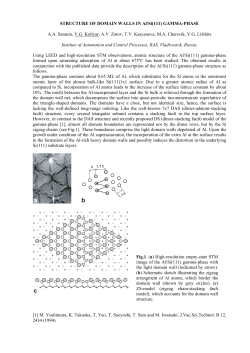


© Copyright 2026