1. No category

Real-Time Forecast Evaluation of DSGE
Models with Nonlinearities
Francis X. Diebold
Frank Schorfheide
University of Pennsylvania
University of Pennsylvania
Minchul Shin
University of Pennsylvania
Preliminary draft
This Version: March 21, 2015
Abstract: Recent work has analyzed the forecasting performance of standard dynamic
stochastic general equilibrium (DSGE) models, but little attention has been given to DSGE
models that incorporate nonlinearities in exogenous driving processes. Against that backgroud, we explore whether incorporating nonlinearities improves DSGE forecasts (point,
interval, and density), with emphasis on stochastic volatility. We examine real-time forecast
accuracy for key macroeconomic variables including output growth, inflation, and the policy
rate. We find that incorporating stochastic volatility in DSGE models of macroeconomic
fundamentals markedly improves their density forecasts, just as incorporating stochastic
volatility in models of financial asset returns improves their density forecasts.
Key words: Dynamic stochastic general equilibrium model, Markov switching, prediction,
stochastic volatility
JEL codes: E17, E27, E37, E47
Acknowledgments: For helpful comments we thank seminar participants at the University
of Pennsylvania and European University Institute, as well as Fabio Canova. For research
support we thank the National Science Foundation and the Real-Time Data Research Center
at the Federal Reserve Bank of Philadelphia.
Contents
1 Introduction
1
2 A Benchmark DSGE Model
2.1 Model Structure . . . . . . . . . . . . . . . . . . . . . . . . . . . . . . . . . .
2.2 Constant vs. Stochastic Shock Volatility . . . . . . . . . . . . . . . . . . . .
1
2
3
3 Model Solution and Estimation
3.1 Transition . . . . . . . . . . .
3.1.1 Constant Volatility . .
3.1.2 Stochastic Volatility .
3.2 Measurement . . . . . . . . .
3.3 Bayesian Estimation . . . . .
.
.
.
.
.
4
4
4
4
5
6
.
.
.
.
.
.
6
7
8
8
8
9
10
.
.
.
.
.
.
10
10
11
12
12
13
14
.
.
.
.
.
.
.
.
.
.
.
.
.
.
.
.
.
.
.
.
.
.
.
.
.
.
.
.
.
.
.
.
.
.
.
.
.
.
.
.
.
.
.
.
.
.
.
.
.
.
.
.
.
.
.
4 Point, Interval and Density Forecast Evaluation
4.1 Predictive Density . . . . . . . . . . . . . . . . .
4.2 Point Forecast Evaluation . . . . . . . . . . . . .
4.3 Interval Forecast Evaluation . . . . . . . . . . . .
4.4 Density Forecast Evaluation . . . . . . . . . . . .
4.4.1 Probability Integral Transforms . . . . . .
4.4.2 Predictive Log Likelihood . . . . . . . . .
5 Empirical Results
5.1 Data Set . . . . . . . . . . . . .
5.2 Estimated Stochastic Volatility
5.3 Point Forecasts . . . . . . . . .
5.4 Interval Forecasts . . . . . . . .
5.5 Density Forecasts . . . . . . . .
5.6 Log Predictive Density . . . . .
.
.
.
.
.
.
.
.
.
.
.
.
.
.
.
.
.
.
.
.
.
.
.
.
.
.
.
.
.
.
.
.
.
.
.
.
.
.
.
.
.
.
.
.
.
.
.
.
.
.
.
.
.
.
.
.
.
.
.
.
.
.
.
.
.
.
.
.
.
.
.
.
.
.
.
.
.
.
.
.
.
.
.
.
.
.
.
.
.
.
.
.
.
.
.
.
.
.
.
.
.
.
.
.
.
.
.
.
.
.
.
.
.
.
.
.
.
.
.
.
.
.
.
.
.
.
.
.
.
.
.
.
.
.
.
.
.
.
.
.
.
.
.
.
.
.
.
.
.
.
.
.
.
.
.
.
.
.
.
.
.
.
.
.
.
.
.
.
.
.
.
.
.
.
.
.
.
.
.
.
.
.
.
.
.
.
.
.
.
.
.
.
.
.
.
.
.
.
.
.
.
.
.
.
.
.
.
.
.
.
.
.
.
.
.
.
.
.
.
.
.
.
.
.
.
.
.
.
.
.
.
.
.
.
.
.
.
.
.
.
.
.
.
.
.
.
.
.
.
.
.
.
.
.
.
.
.
.
.
.
.
.
.
.
.
.
.
.
.
.
.
.
.
.
.
.
.
.
.
.
.
.
.
.
.
.
.
.
.
.
.
.
.
.
.
.
.
.
6 Concluding Remarks
14
A Log Predictive Score
A-1
1
Introduction
Dynamic stochastic general equilibrium (DSGE) models are now used widely for forecasting.
Recently, several studies have shown that standard linearized DSGE models compete successfully with other forecasting models, including linear reduced-form time-series models such as
vector autoregressions (VAR’s).1 However, little is known about the predictive importance
of omitted non-linearities. Recent work by Sims and Zha (2006), Justiniano and Primiceri
(2008), Bloom (2009), and Fern´andez-Villaverde and Rubio-Ram´ırez (2013) has highlighted
that time-varying volatility is one of the key nonlinearities not just in financial data but also
in macroeconomic time series. Against this background, we examine the real-time forecast
accuracy (point, interval and density) of linearized DSGE models with and without stochastic volatility. We seek to determine whether and why incorporation of stochastic volatility
is helpful for macroeconomic forecasting.
Several structural studies find that density forecasts from linearized standard DSGE
models are not well-calibrated, but they leave open the issue of whether simple inclusion of
stochastic volatility would fix the problem.2 Simultaneously, reduced-form studies such as
Clark (2011) clearly indicate that inclusion of stochastic volatility in linear models (vector
autoregressions) improves density forecast calibration. Our work in this paper, in contrast,
is structural and yet still incorporates stochastic volatility, effectively asking questions in the
tradition of Clark (2011), but in a structural environment.
We proceed as follows. In Section 2 we introduce a benchmark DSGE model, with and
without stochastic volatility. In Section 3 we describe our model solution and estimation
methods. In Section 4 we present aspects of point, interval and density forecasting and
forecast evaluation. In Section 5 we provide empirical results on comparative real-time
forecasting performance. We conclude in Section 6.
2
A Benchmark DSGE Model
Here we present our benchmark model and its equilibrium conditions. It is a small-scale New
Keynesian model studied by An and Schorfheide (2007) and Herbst and Schorfheide (2012).
1
See, for example, the survey of Del Negro and Schorfheide (2013).
See Pichler (2008), Bache et al. (2011), Herbst and Schorfheide (2012), Del Negro and Schorfheide (2013)
and Wolters (2015).
2
2.1
Model Structure
The model economy consists of households, firms, a central bank that conducts monetary
policy by setting the nominal interest rate, and a fiscal authority that determines the amount
of government consumption and finances it using lump-sum taxes. In what follows, we are
summarizing the equilibrium conditions of this economy. Technology At evolves according
to
log At = log γ + log At−1 + zt .
(1)
On average technology grows at rate γ, with exogenous fluctuations driven by zt . The
stochastic trend in technology induces stochastic trend in equilibrium output and consumption. The model economy has a unique deterministic steady state in terms of detrended
variables ct = Ct /At and yt = Yt /At , where Ct and Yt are consumption and output, respectively.
The households determine their supply of labor services to the firms and choose consumption. They receive labor and dividend income as well interest rate payments on nominal
bonds. The consumption Euler equation is
1 = βEt
τ
ct
ct+1
Rt
,
πt+1 ezt+1
(2)
where ct is consumption, Rt is the gross nominal interest rate, and πt = Pt /Pt−1 is gross
inflation. The parameter τ captures the relative degree of risk aversion and β is a discount
factor for the representative household.
The production sector consists of monopolistically competitive intermediate-goods producing firms and perfectly competitive final goods producers. The former hire labor from
the household, produce their goods using a linear technology with productivity At , and sell
their output to the final goods producers. Nominal price rigidities are introduced by assuming that the intermediate-goods producers face quadratic price adjustment costs. The final
goods producers simply combine the intermediate goods. In equilibrium the inflation in the
price of the final good evolves according to
π
ct τ yt+1
1 τ
1
πt +
= βEt
πt+1 (πt+1 − π) +
(c + ν − 1)) ,
(πt − π) 1 −
2ν
2ν
ct+1
yt
νφ t
(3)
where φ governs the price stickiness in the economy, 1/ν is the elasticity of demand for each
intermediate good, and π is the steady-state inflation rate associated with the final good.
Log-linarizing this equation leads to the New Keynesian Phillips curve. The larger the price
adjustment costs φ, the flatter the Phillips curve.
2
We assume that a fraction of output is used for government consumption and write
y t = ct e g t ,
(4)
where gt is an exogenously evolving government spending shock. Market clearing and the
aggregate resource constraint imply
φ
−gt
2
ct = yt e − (πt − π) .
2
(5)
The first term in brackets captures the fraction of output that is used for government consumption and the second term captures the loss of output due to the nominal price adjustment costs. The central bank policy rule reacts to inflation and output growth,
"
ρR
Rt = Rt−1
ψ2
π ψ1 y
t
t
z
e
π
γyt−1 t
#1−ρR
em
t ,
(6)
where mt is a monetary policy shock.
2.2
Constant vs. Stochastic Shock Volatility
We complete the model by specifying the exogenous shock processes,
mt = σR,t R,t
(7)
zt = ρz zt−1 + σz,t z,t
(8)
gt = (1 − ρg ) log g + ρg gt−1 + σg,t g,t .
(9)
We assume that R,t , z,t , and g,t are orthogonal at all leads and lags, and normally distributed with zero means and unit variances.
In a constant-volatility implementation, we simply take σR,t = σR , σz,t = σz and σg,t =
σg . Incorporating stochastic volatility is similarly straightforward. Following Fern´andezVillaverde and Rubio-Ram´ırez (2007), Justiniano and Primiceri (2008), and Fern´andezVillaverde and Rubio-Ram´ırez (2013), we take
σi,t = σi ehi,t
hi,t = ρσi hi,t−1 + νi,t
3
where νi,t and i,t are orthogonal at all leads and lags, for all i = R, z, g and t = 1, ..., T .
3
Model Solution and Estimation
Equations (2)-(9) form a non-linear rational expectations system. The implied equilibrium
law of motion can be written as
st = Φ(st−1 , t ; θ)
where st is a vector of state variables (st = [yt , ct , πt , Rt , mt , gt , zt ]), t is a vector of structural
shock innovations, and θ is a vector of model parameters. In general there is no closedform solution, so the model must be solved numerically. The most popular approach is
linearization of transition and measurement equations; that is, use of first-order perturbation
methods. The first-order perturbation approach yields a linear state-space system that can
be analyzed with the Kalman filter.
3.1
Transition
We present transition equations with constant and stochastic volatility.
3.1.1
Constant Volatility
First-order perturbation results in the following linear transition equation for the state variables,
st = H1 (θ)st−1 + R(θ)t
t ∼ iidN (0, Q(θ)),
(10)
where H1 is a ns × ns matrix, R is a ns × ne matrix and Q is a ne × ne matrix, where ns
is the number of state variables and ne is the number of structural shocks. The elements of
the coefficient matrices (H1 (θ), R(θ), Q(θ)) are non-linear functions of θ.
3.1.2
Stochastic Volatility
Linearization is inappropriate with stochastic volatility, as stochastic volatility vanishes under linearization. Instead, at least second-order approximation is required to preserve terms
related to stochastic volatility, as shown by Fern´andez-Villaverde and Rubio-Ram´ırez (2007,
4
2013). Interestingly, however, Justiniano and Primiceri (2008) suggest a method to approximate the model solution using a partially non-linear function. The resulting law of motion
is the same as that of the linearized solution, except that the variance-covariance matrix of
the structural shocks can be time-varying,
st = H1 (θ)st−1 + R(θ)t
t ∼ iidN (0, Qt (θ)).
(11)
More specifically, Qt (θ) is a diagonal matrix with elements e2hi,t , where each hi,t has its own
transition,
hi,t = ρσi hi,t−1 + νi,t
νi,t ∼ iidN (0, s2i ),
(12)
for i = R, g, z. Together with a measurement equation, equations (11) and (12) form a
partially non-linear state-space representation. One of the nice features of this formulation
is that the system remains linear and Gaussian, conditional on Qt .
3.2
Measurement
We complete the model with a set of measurement equations that connect state variables to
observable variables. We consider quarter-on-quarter per capita GDP growth rates (Y GR)
and inflation rates (IN F ), and quarterly nominal interest (federal funds) rates (F F R). We
measure IN F and F F R as annualized percentages, and we measure YGR as a quarterly
percentage. We assume that there is no measurement error. Then the measurement equation
is
Y GRt = 100 log(yt − yt−1 + zt )
IN Ft = 400 log πt
(13)
F F Rt = 400 log Rt .
In slight abuse of notation we write the measurement equation as
Yt = Z(θ)st + D(θ),
5
(14)
where Yt is now the n × 1 vector of observed variables (composed of Y GRt , IN Ft , and
F F Rt ), Z(θ) is an n × ns matrix, st is the ns × 1 state vector, and D(θ) is an n × 1 vector
that usually contains the steady-state values of the corresponding model state variables.
3.3
Bayesian Estimation
We perform inference and prediction using the Random Walk Metropolis (RWM) algorithm
with the Kalman filter, as facilitated by the linear-Gaussian structure of our state-space
system, conditional on Qt . In particular, we use the Metropolis-within-Gibbs algorithm
developed by Kim et al. (1998) to generate draws from the posterior distribution.
Implementing Bayesian techniques requires the specification of a prior distribution. We
use priors consistent with those of Del Negro and Schorfheide (2013) for parameters that
we have in common. We take the prior for the price-stickiness parameter from Herbst
and Schorfheide (2012). Because ν (elasticity of demand) and φ (price stickiness) are not
separately identified in the linear DSGE model, we fix ν at 0.1, we estimate φ via κ, the
slope of the Phillips curve.3
For the model with stochastic volatility, we specify prior distributions as:
ρσi ∼ N (0.9, 0.07),
s2i ∼ IG(2, 0.05)
for i = R, g, z. We constrain the priors for the AR(1) stochastic-volatility coefficients to be
in the stationary region, ρσi ∈ (−1, 1). We set the prior mean for the variances of volatility
shocks in line with the higher value used by Clark (2011), rather than the very low value
used by Primiceri (2005) and Justiniano and Primiceri (2008).
We summarize the complete list of prior distributions in Table 1.
4
Point, Interval and Density Forecast Evaluation
In this section, we discuss how to measure the forecasting accuracy based on the predictive
density of YT +1:T +H = {YT +1 , . . . , YT +H } given the information available at time T . First,
we discuss how to generate draws from the predictive distribution based on the posterior
draws p(θ|Y1:T ). Second, we discuss measures of point and density forecast accuracy.
3
1−ν
κ is defined as κ = τ νπ
2φ .
6
4.1
Predictive Density
We generate draws from the posterior predictive distribution based on the following decomposition,
p(YT +1:T +H |Y1:T )
Z
= p(YT +1:T +H |θ, Y1:T )p(θ|Y1:T )dθ
"Z
Z
#
(15)
p(YT +1:T +H |sT +1:T +H )p(sT +1:T +H |sT , θ, Y1:T )dsT +1:T +H
=
(sT ,θ)
sT +1:T +H
× p(sT |θ, Y1:T )p(θ|Y1:T )d(sT , θ).
This decomposition shows that the predictive density reflects parameter uncertainty p(θ|Y1:T ),
uncertainty about sT conditional on Y1:T , p(sT |θ, Y1:T ), and uncertainty about the future realization of shocks that determine the evolution of the states, p(sT +1:T +H |sT , θ, Y1:T ). For
instance, draws from the predictive density for the linear DSGE model can be generated
with the following algorithm:
Algorithm (Del Negro and Schorfheide (2013)):
For j = 1 to M , select the j’th draw from the posterior distribution p(θ|Y1:T ) and:
1. Use the Kalman filter to compute mean and variance of the distribution P (sT |θ(j) , Y1:T ).
(j)
Generate a draw sT from this distribution.
2. Obtain a draw from p(sT +1:T +H |sT , θ, Y1:T ) by generating a sequence of innovations
(j)
(j)
T +1:T +H . Then, starting from sT , iterate the state transition equation (10) with θ
(j)
replaced by the draw θ(j) forward to obtain a sequence sT +1:T +H :
(j)
(j)
(j)
st = H1 (θ(j) )st−1 + R(θ(j) )t ,
t = T + 1, ..., T + H.
(j)
3. Use the measurement equation (14) to obtain YT +1:T +H :
(j)
Yt
(j)
= D(θ(j) ) + Z(θ(j) )st ,
(j)
t = T + 1, ..., T + H.
The algorithm produces M trajectories YT +1:T +H from the predictive distribution of YT +1:T +H
given Y1:T . In our application, we generate 20,000 draws from the posterior distribution
7
P (θ|Y1:T ). Then we discard the first 5,000 draws and select every 15th draws to get M =
1, 000. For each j = 1, . . . , 1, 000, we repeat steps 2 and 3 15 times, which produces a total
of 15, 000 draws from the predictive distribution.
4.2
Point Forecast Evaluation
We treat the mean of the posterior predictive distribution as a point forecast. We compute
it by a Monte Carlo average,
YˆT +h|T =
Z
YT +h p(YT +h |Y1:T )dYT +h ≈
YT +h
nsim
1 X
nsim
(j)
YT +h .
j=1
This is the optimal predictor under the quadratic loss.
To evaluate the performance of the point forecast from various DSGE models, we compare
RMSEs,
v
uR+P −h
X
1 u
t
(Yi,t+h − Yˆi,t+h|t )2
RM SE(i|h) =
P −h
t=R
where R (“regression sample”) is the index denotes the starting point of the forecasts evaluation sample and P (“prediction sample”) the number of forecasting origins.
4.3
Interval Forecast Evaluation
Interval Forecasts If the forecast density is well calibrated, the probabilistic statement
based on the credible set derived from this density should be consistent with data. For
example, actual variables are expected to be inside of 1 − α% credible interval forecasts at
the same frequency α%. If the frequency is greater than (less than) α%, the posterior density
is too wide narrow). We compute interval forecasts for a particular element Yi,T +h of YT +h
by numerically searching for the shortest connected interval that contains a 1 − α fraction
(j)
of the draws {Yi,T +h }M
j=1 (the highest-density set).
4.4
Density Forecast Evaluation
To evaluate density forecasts, we use an absolute standard, the probability integral transform,
and a relative standard, the log predictive density.
8
The first checks whether the individual predictive distributions are well calibrated.4 The
second compares overall calibration of the density forecasts.
4.4.1
Probability Integral Transforms
The probability integral transform (PIT) of yi,T +h based on time T predictive distribution
is defined as the cumulative density of the random variable yi,T +h evaluated at the true
realization of Yi,T +h ,
Z Yi,T +h
p(Y˜i,T +h |Y1:T )dY˜i,T +h .
zi,h,T =
−∞
We compute PITs by the Monte Carlo average of the indicator function,
zi,h,T
M
1 X
(j)
I{Yi,T +h ≤ Yi,T +h }.
≈
M j=1
If the predictive distribution is well-calibrated, zi,h,T should follow the uniform distribution.
Moreover, for h = 1, zi,h,T ’s are independent across time and uniformly distributed. (Diebold
et al. (1998)).
We can further transform PIT’s by the inverse of the standard normal distribution function,
wi,h,T = Φ−1 (zi,h,T )
where Φ−1 (·) is the inverse of the standard normal distribution function. This quantity
for h = 1 is called normalized forecasts error. The normalized forecasts error should be
an independent standard normal random variable. To evaluate the density forecasts, we
compare means, standard deviations, autocorrelations of normalized forecasts error from
various models and consider the test based on the likelihood ratio (LR test) developed by
Berkowitz (2001).
4
A predictive distribution is well calibrated if the predicted probabilities of events are consistent with
their observed frequencies. See Del Negro and Schorfheide (2013) and Herbst and Schorfheide (2012).
9
4.4.2
Predictive Log Likelihood
The predictive log likelihood can be used to compare the quality of probabilistic forecasts.
Following Warne et al. (2012), we compute the log predictive likelihood as follows:
R+P
X−h
1
log p(Yt+h |Y1:t , m),
SM (h, m) =
P − h t=R
h = 1, 2, ..., H
(16)
where H is the maximum forecasting horizon. Here m stands for ‘marginal’ as opposed to
the ‘joint’ predictive score which is defined as
R+P
X−h
1
SJ (h, m) =
log p(Yt+1:t+h |Y1:t , m),
P − h t=R
h = 1, 2, ..., H.
The marginal predictive score has a nice interpretation. To see this we decompose p(·) in
the equation (16)
p(Yt+h , Y1:t )
p(Yt+h |Y1:t ) =
, h = 1, 2, ..., H
p(Y1:t )
which is a ratio of the marginal density with (Yt+h , Y1:t ) to only with (Y1:t ). Obviously when
h = 1, two concepts lead to the same quantity.
5
Empirical Results
We first discuss data set used in this paper. Then, we report our empirical findings.
5.1
Data Set
For the evaluation of point and density forecasts, we use the real-time data set constructed
by Del Negro and Schorfheide (2013).5 They compare the point forecasts from the DSGE
model to those from the Bluechip survey and Federal Reserve Board’s Greenbook. To make
forecasts from the DSGE models comparable to the real-time forecasts made in Bluechip
survey and Greenbook, they built data vintages that are aligned with the publication dates
of the Blue Chip survey and the Federal Reserve Board’s Greenbook. In this study, we use
the data set matched with the Blue Chip survey publication dates.
The first forecast origin considered in the forecast evaluation is (two weeks prior to)
5
The same data set used in Herbst and Schorfheide (2012).
10
January 1992 and the last forecast origin for one-step-ahead forecasts is (two weeks prior
to) April 2011. As in Del Negro and Schorfheide (2013), we use data vintages in April,
July, October, and January. Hence we make use of four data vintages per year and the total
number of data vintages used in this study is 78. The estimation sample starts from 1964:Q2
for all vintages. Following Del Negro and Schorfheide (2013), we compute forecast errors
based on actuals that are obtained from the most recent vintage hoping that these are closer
to the “true” actuals6 . 7
To evaluate forecasts we recursively estimate DSGE models over the 78 vintages starting
from the January 1992 vintage. That is, for the January 1992 vintage we estimate DSGE
models with sample from 1964:Q2 to 1991:Q3 and generate forecasts for 1991:Q4 (onestep-ahead) ∼ 1993:Q2 (eight-steps-ahead). We iterate this procedure for all vintages from
January 1992 to April 2011.
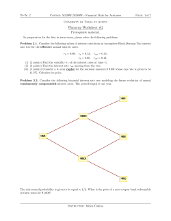
5.2
Estimated Stochastic Volatility
For the DSGE model with stochastic volatility to produce density forecasts more accurate
than constant volatility DSGE models, the estimated variances of structural shocks should
change significantly over time. Therefore, as a starting point, we overlay and compare
estimated variances for structural shocks from the constant volatility DSGE model and
stochastic volatility DSGE model. Figure 1 reports estimates (posterior means) obtained
with different real-time data vintages. The stochastic volatility estimates (solid line) and
constant volatility estimate (dotted line) are obtained with data samples ending in 1991:Q3,
2001:Q3, and 2010:Q3 (obtained from data vintages of January 1992, January 2002, and
January 2011, respectively). Overall, the estimates confirm significant time variation in
volatility. In particular, volatility fell sharply in the mid-1980s with the Great Moderation.
The estimates also reveal a sharp rise in volatility in recent years (for volatility on the
technology shock). The general shapes of volatility are very similar across vintages, but level
can differ slightly. Standard deviation estimates from the constant volatility DSGE model
overstate the standard deviations for the post-Great Moderation period because the model
tries to balance out the effect of the high variance before the 80s. Estimates are decreasing as
we include more data from the Great Moderation, but they are still larger than the estimates
6
Alternatively, we could have used actuals from the first “final” data release, which for output corresponds
to the “Final” NIPA estimate (available roughly three months after the quarter is over). Del Negro and
Schorfheide (2013) found that the general conclusions about the forecast performance of DSGE models are
not affected by the choice of actuals. Similar conclusion is made in Rubaszek and Skrzypczy´
nski (2008).
7
More details on the data set can be found in the Del Negro and Schorfheide (2013).
11
from the model with stochastic volatility.
5.3
Point Forecasts
Figure 2 and Table 2 present real-time forecasts RMSEs for 1991:Q4-2011:Q1. Table 2
includes RMSEs for constant variance linearized DSGE model (benchmark) forecasts and
ratios of RMSEs for stochastic volatility DSGE model. In these blocks, entries with value
of less than 1 mean that a forecast is more accurate than the benchmark model. To provide
a rough measure of statistical significance, Table 2 presents p-values for the null hypothesis
that the MSE of a given model is equal to the MSE of the constant volatility linearized
DSGE model, against the (one-sided) alternative that the MSE of the given model is lower.
These p-values are obtained by comparing the tests of Diebold and Mariano (1995) against
standard normal critical values.
The model with stochastic volatility tends to generate more accurate point forecasts for
output growth especially in the short-run. It also has a smaller RMSE for the interest rate in
the very short horizon (h = 1). However, inflation forecasts are very similar across models.
In general, RMSEs of the DSGE model with stochastic volatility get closer to the constant
variance DSGE model as the horizon increases.
5.4
Interval Forecasts
Table 3 reports the frequency with which real-time outcomes for output growth, inflation
rate, and the federal funds rate fall inside 70% highest posterior density intervals estimated
in real time with the DSGE models. Accurate intervals should produce frequencies of about
70%. A frequency of greater than (less than) 70% means that on average over a given
sample, the posterior density is too wide (narrow). The table includes p-values for the null
of correct coverage (empirical = nominal rate of 70%), based on t-statistics. These p-values
are provided as a rough gauge of the importance of deviations from correct coverage.
As Table 3 shows, the constant variance DSGE models tend to be too wide, with actual
outcomes falling inside the intervals much more frequently than the nominal 70% rate. For
example, for the one-step-ahead forecast horizon, the linearized DSGE model coverage rates
range from 91% to 95%. Based on the reported p-values, all of these departures from the
nominal coverage rate appear to be statistically meaningful. For all cases, coverage rates
are much wider than the nominal rate, meaning that the constant volatility DSGE model
overestimates the uncertainty in the predictive distribution.
12
Adding stochastic volatility to the DSGE model improves the calibration of the interval
forecasts with coverage rates closer to the nominal rate than the constant variance DSGE
models. For example, at horizon one, coverage rate for output growth deceases to 77% from
95%. However, they are still somewhat higher for some cases having coverage rates higher
than 80%.
5.5
Density Forecasts
Figure 3 and 4 report histograms of probability integral transformation (PIT) for horizon
1 and 4, respectively. PITs are grouped into five equally sized bins. Under a uniform
distribution, each bin should contain 20% of the PITs, indicated by the solid horizontal lines
in the figure. For output growth, large fraction of PITs fall into 0.4-0.8 bins, indicating that
the predictive distribution is too diffuse. PITs for inflation rate and federal funds rate have
a similar problem. Tails are not covered and too few fractions of PITs are in the 0-0.2 bin
(left tail) for inflation rate or in the 0.8-1 bin (right tail) for federal funds rate, showing that
uncertainty is overestimated by the density forecasts. For longer horizon (h = 4), histograms
for federal fund rate becomes closer to the uniform distribution, but still only a small fraction
of PITs fall into the 0.8-1 bin (right tail).
The inclusion of stochastic volatility to the DSGE model substantially improves the
calibration of the density forecasts. The PIT histograms are more close to that of the
uniform distribution. For example, at horizon 1, PITs for output growth tend to be equally
distributed. More PITs are distributed on the tail for both inflation rate and federal funds
rate. Although the discrepancy between histograms and the horizontal line become larger
as the horizon increases, they are closer to the uniform distribution than in the constant
volatility case.
For a more formal assessment, Table 6 reports various test metrics, including the standard deviations of the normalized error, along with p-values for the null that the standard
deviation equals 1; the means of the normalized errors, along with p-values for the null of
a zero mean; the AR(1) coefficient estimate and its p-value, obtained by a least squares
regression including a constant; and the p-value of Berkowitz (2001)’s likelihood ratio test
for the joint null of zero mean, unity variance, and no AR(1) serial correlation.
The tests confirm that without stochastic volatility, standard deviations are much less
than 1, means are sometimes nonzero, and serial correlation can be considerable. For example, standard deviations of normalized forecast errors from the constant volatility DSGE
model are at most 0.58 for output growth and federal funds rate; the corresponding p-values
13
are all close to 0. For inflation rate, standard deviations are slightly larger but still smaller
than 1. The absolute values of AR (1) coefficients range from 0.12 to 0.66, with p-values
close to 0 except in the case of inflation for which the p-value is 0.47. Not surprisingly,
given the results for means, standard deviations, and AR (1) coefficients, the p-values of the
Berkowitz (2001) test are nearly 0.
By allowing stochastic volatility, the quality of density forecasts is improved based on
the formal metrics. The standard deviations of the normalized forecast errors are all greater
than 0.8 with p-values of 0.349 or greater. Means are all close to zero, whereas the means for
output growth from the constant volatility DSGE model are around 0.2, with p-value smaller
than 0.005. The patterns for AR (1) coefficients are similar to the constant volatility case,
except for inflation rate (no AR (1) serial correlation). Due to the high AR (1) coefficient,
p-values for LR tests are also nearly 0 for output growth and federal funds rate, even after
adding the stochastic volatility.
5.6
Log Predictive Density
Table 7 presents the average log predictive densities (from one-step-ahead to eight-stepahead). The model with stochastic volatility has a substantially larger value, which again
confirms that the density forecasts are improved by including stochastic volatility (h = 1).
However, as h increases constant volatility model has larger log predictive density. Figure 5
shows the time-series plot of the one-step-ahead and four-step-ahead log predictive densities.
For most of the time, the one-step-ahead predictive densities of the model with stochastic
volatility are higher than the constant volatility DSGE model.
6
Concluding Remarks
We have examined the accuracy of point, interval and density forecasts of output growth, inflation, and the federal funds rate, generated from DSGE models with and without stochastic
volatility. Including stochastic volatility produces large improvements in interval and density
forecasts, and even some improvement in point forecasts.
14
References
An, S. and F. Schorfheide (2007), “Bayesian Analysis of DSGE Models,” Econometric Reviews, 26, 113–172.
Bache, W. I., S.A.. Jore, J. Mitchell, and S.P. Vahey (2011), “Combining VAR and DSGE
Forecast Densities,” Journal of Economic Dynamics and Control .
Berkowitz, J. (2001), “Testing Density Forecasts, With Applications to Risk Management,”
Journal of Business and Economic Statistics, 19, 465–474.
Bloom, N. (2009), “The Impact of Uncertainty Shocks,” Econometrica, 77, 623–685.
Clark, T.E. (2011), “Real-Time Density Forecasts From Bayesian Vector Autoregressions
With Stochastic Volatility,” Journal of Business and Economic Statistics, 29, 327–341.
Del Negro, Marco and Frank Schorfheide (2013), “DSGE Model-Based Forecasting,” in
“Handbook of Economic Forecasting,” (edited by Elliott, Graham and Allan Timmermann), 2, forthcoming, North Holland, Amsterdam.
Diebold, F.X., T.A. Gunther, and A.S. Tay (1998), “Evaluating Density Forecasts with
Applications to Financial Risk Management,” International Economic Review , 39, pp.
863–883.
Diebold, F.X. and R.S. Mariano (1995), “Comparing Predictive Accuracy,” Journal of Business and Economic Statistics, 13, 253–263.
Fern´andez-Villaverde, Jes´
us and Juan F. Rubio-Ram´ırez (2007), “Estimating Macroeconomic
Models: A Likelihood Approach,” Review of Economic Studies, 74, 1059–1087.
Fern´andez-Villaverde, Jes´
us and Juan F. Rubio-Ram´ırez (2013), “Macroeconomics and
Volatility: Data, Models, and Estimation,” in “Advances in Economics and Econometrics: Tenth World Congress,” (edited by Acemoglu, D., M. Arellano, and E Dekel), 3,
137–183, Cambridge University Press.
Herbst, E. and F. Schorfheide (2012), “Evaluating DSGE Model Forecasts of Comovements,”
Journal of Econometrics.
Justiniano, A. and G.E. Primiceri (2008), “The Time-Varying Volatility of Macroeconomic
Fluctuations,” American Economic Review , 98, 604–41.
15
Kim, S., N. Shephard, and S. Chib (1998), “Stochastic Volatility: Likelihood Inference and
Comparison With ARCH Models,” The Review of Economic Studies, 65, 361–393.
Pichler, P. (2008), “Forecasting with DSGE Models: The Role of Nonlinearities,” The B.E.
Journal of Macroeconomics, 8, 20.
Primiceri, G.E. (2005), “Time Varying Structural Vector Autoregressions and Monetary
Policy,” Review of Economic Studies, 72, 821–852.
Rubaszek, M. and P. Skrzypczy´
nski (2008), “On the Forecasting Performance of a SmallScale DSGE Model,” International Journal of Forecasting, 24, 498–512.
Sims, C.A. and T. Zha (2006), “Were There Regime Switches in U.S. Monetary Policy?”
American Economic Review , 96, 54–81.
Warne, A., G. Coenen, and K. Christoffel (2012), “Forecasting with DSGE-VAR Models,” .
Wolters, M.H. (2015), “Evaluating Point and Density Forecasts of DSGE Models,” Journal
of Applied Econometrics, 30, 74–96.
16
Tables and Figures
Table 1: Priors for structural parameters of DSGE model
Parameter
τ
ν
κ
1/g
ψ1
ψ2
ρr
ρg
ρz
400 log(1/β)
400 log π
100 log γ
Distribution Para (1)
Gamma
Beta
Gamma
Fixed
Gamma
Gamma
Beta
Beta
Beta
Gamma
Gamma
Normal
2
0.1
0.2
0.85
1.5
0.12
0.75
0.5
0.5
1
2.48
0.4
Para (2)
0.5
0.05
0.1
N/A
0.25
0.05
0.1
0.2
0.2
0.4
0.4
0.1
Parameter Distribution Para (1)
100σr
100σg
100σz
ρσr
ρσg
ρσz
100σσr
100σσg
100σσz
InvGamma
InvGamma
InvGamma
Normal
Normal
Normal
InvGamma
InvGamma
InvGamma
0.3
0.4
0.4
0.9
0.9
0.9
2.5
2.5
2.5
Para (2)
4
4
4
0.07
0.07
0.07
4
4
4
Notes: 1. For the linear DSGE models and the model with stochastic volatility, we fix ν at 0.1.
2. Para (1) and Para(2) list the means and the standard deviations for Beta, Gamma, and Normal distributions; the upper and lower bound of the support for the Uniform distribution; and s and ν for the Inverse
2
2
Gamma distribution, where pIG (σ|ν, s) ∝ σ −ν−1 e−νs /2σ .
17
Table 2: Real-time forecast RMSEs, 1991Q4-2011Q1
h = 1Q
h = 2Q
h = 4Q
h = 8Q
0.704
0.948 (0.136)
0.723
0.983 (0.396)
(a) Output Growth
Linear
Linear+SV
0.682
0.933 (0.017)
0.696
0.938 (0.089)
(b) Inflation Rate
Linear
Linear+SV
0.263
1.021 (0.942)
0.265
1.032 (0.845)
0.299
1.045 (0.821)
0.339
1.025 (0.632)
(c) Fed Funds Rate
Linear
Linear+SV
0.157
0.944 (0.004)
0.262
0.966 (0.148)
0.406
1.000 (0.497)
0.547
1.047 (0.921)
Notes : 1. RMSEs for benchmark DSGE model in the first panel, RMSE ratios in all others. a) Linear: the
linear DSGE model with constant volatility. b) Linear+SV: the DSGE model with stochastic volatility using
the method proposed by Justiniano and Primiceri (2008).
2. The forecast errors are calculated using actuals that are obtained from the most recent vintage.
3. p-values of t-tests of equal MSE, taking the linear DSGE models with constant volatilities as the benchmark,
are given in parentheses. These are one-sided Diebold-Mariano tests, of the null of equal forecast accuracy
against the alternative that the non-benchmark model in question is more accurate. The standard errors
entering the test statistics are computed with the Newey-West estimator, with a bandwidth of 0 at the 1quarter horizon and n1/3 in the other cases. n is the number of forecasting origins.
18
Table 3: Real-time forecast coverage rates, 1991Q4-2011Q1 (70%)
h = 1Q
h = 2Q
h = 4Q
h = 8Q
(a) Output Growth
Linear
0.949 (0.000) 0.909 (0.000) 0.893 (0.000) 0.914 (0.000)
Linear+SV 0.769 (0.147) 0.779 (0.149) 0.800 (0.040) 0.829 (0.106)
(b) Inflation Rate
Linear
0.872 (0.000) 0.857 (0.002) 0.947 (0.000) 0.943 (0.000)
Linear+SV 0.782 (0.079) 0.779 (0.135) 0.853 (0.004) 0.857 (0.032)
(c) Fed Funds Rate
Linear
0.936 (0.000) 0.896 (0.000) 0.827 (0.066) 0.800 (0.324)
Linear+SV 0.846 (0.000) 0.701 (0.986) 0.640 (0.499) 0.600 (0.343)
Notes: 1. a) Linear: the linear DSGE model with constant volatility. b) Linear+SV: the DSGE model with
stochastic volatility using the method proposed by Justiniano and Primiceri (2008).
2. The table reports the frequencies with which actual outcomes fall within 70 percent bands computed from
the posterior distribution of forecasts.
3. The table includes in parentheses p-values for the null of correct coverage (empirical = nominal rate of
70 percent), based on t-statistics using standard errors computed with the Newey-West estimator, with a
bandwidth of 0 at the 1-quarter horizon and n1/3 in the other cases. n is the number of forecasting origins.
19
Table 4: Real-time forecast coverage rates (LR Test), 1991Q4-2011Q1 (70%)
h = 1Q
h = 2Q
h = 4Q
h = 8Q
(a) Output Growth
Linear
0.949 (0.000) 0.909 (0.000) 0.893 (0.000) 0.914 (0.002)
Linear+SV 0.769 (0.171) 0.779 (0.118) 0.800 (0.049) 0.829 (0.080)
(b) Inflation Rate
Linear
0.872 (0.000) 0.857 (0.001) 0.947 (0.000) 0.943 (0.000)
Linear+SV 0.782 (0.103) 0.779 (0.118) 0.853 (0.002) 0.857 (0.030)
(c) Fed Funds Rate
Linear
0.936 (0.000) 0.896 (0.000) 0.827 (0.012) 0.800 (0.180)
Linear+SV 0.846 (0.003) 0.701 (0.980) 0.640 (0.265) 0.600 (0.209)
Notes: 1. a) Linear: the linear DSGE model with constant volatility. b) Linear+SV: the DSGE model with
stochastic volatility using the method proposed by Justiniano and Primiceri (2008).
2. The table reports the frequencies with which actual outcomes fall within 70 percent bands computed from
the posterior distribution of forecasts.
3. The table includes in parentheses p-values for the null of correct coverage (empirical = nominal rate of
70 percent), based on the LR test.
20
Table 5: Real-time 70% interval forecast (1-step-ahead) LR test, 1991Q42011Q1
Coverage
Independence
(a) Output Growth
Linear
30.87 (0.000) 1.92 (0.165)
Linear+SV 1.87 (0.171)
0.25 (0.619)
(b) Inflation Rate
Linear
12.85 (0.000) 0.67 (0.413)
Linear+SV 2.66 (0.103)
0.65 (0.420)
(c) Fed Funds Rate
Linear
26.97 (0.000) 1.11 (0.292)
Linear+SV 9.00 (0.003)
9.98 (0.002)
Joint
32.89 (0.000)
2.65 (0.266)
13.79 (0.001)
3.80 (0.149)
28.21 (0.000)
19.32 (0.000)
Notes: 1. a) Linear: the linear DSGE model with constant volatility. b) Linear+SV: the DSGE model with
stochastic volatility using the method proposed by Justiniano and Primiceri (2008).
2. The table reports the frequencies with which actual outcomes fall within 70 percent bands computed from
the posterior distribution of forecasts.
3. The table includes in parentheses p-values for the null of correct coverage (empirical = nominal rate of
70 percent), based on the LR test.
21
Table 6: Tests of normalized errors of 1-step ahead real-time forecasts
Std. Dev.
Mean
AR(1) coef.
LR test
(a) Output Growth
Linear
0.537 (0.000)
Linear+SV 0.827 (0.349)
0.194 (0.004)
0.093 (0.493)
0.349 (0.026)
0.254 (0.072)
53.740 (0.000)
10.610 (0.014)
(b) Inflation Rate
Linear
0.763 (0.324)
Linear+SV 0.868 (0.461)
0.059 (0.590)
0.130 (0.368)
-0.121 (0.492) 10.467 (0.015)
-0.000 (0.998) 3.915 (0.271)
(c) Fed Funds Rate
Linear
0.583 (0.000) -0.074 (0.646)
Linear+SV 0.866 (0.492) -0.119 (0.593)
0.658 (0.000)
0.744 (0.000)
76.000 (0.000)
66.514 (0.000)
Notes: 1. Forecasting periods: 1991Q4-2011Q1. a) Linear: the linear DSGE model with constant volatility.
b) Linear+SV: the DSGE model with stochastic volatility using the method proposed by Justiniano and
Primiceri (2008).
2. The normalized forecast error is defined as Φ−1 (zt+1 ), where zt+1 denotes the PIT of the one-step ahead
forecast error and Φ−1 is the inverse of the standard normal distribution function.
3. The first column reports the estimated standard deviation of the normalized error, along with a p-value
for a test of the null hypothesis of a standard deviation equal to 1 (computed by a linear regression of the
squared error on a constant, using a Newey-West variance with 3 lags.). The second column reports the mean
of the normalized error, along with a p-value for a test of the null of a mean of zero (using a Newey-West
variance with 5 lags). The third column reports the AR(1) coefficient and its p-value, obtained by estimating
an AR(1) model with an intercept (with heteroskedasticity-robust standard errors). The final column reports
the $p$-value of Berkowitz’s (2001) likelihood ratio test for the joint null of a zero mean, unity variance, and
no [AR(1)] serial correlation.
22
Table 7: Log Predictive Score, 1991Q4-2011Q1
Linear
Linear+SV
h = 1Q
h = 2Q
h = 4Q
h = 8Q
-3.99
-3.82
-4.20
-4.66
-4.91
-5.70
-6.55
-6.65
Notes: 1. a) Linear: the linear DSGE model with constant volatility. b) Linear+SV: the DSGE model with
stochastic volatility using the method proposed by Justiniano and Primiceri (2008).
2. Log predictive scores are defined and computed as in Warne et al. (2012). See appendix for detail.
23
Figure 1: Estimated Time Varying Standard Deviations
Vintage at January 1992
Vintage at January 2002
Vintage at January 2011
Notes: Posterior means (solid line) and 80% confidence bands (shaded area) of standard deviations of the
structural shocks based on the DSGE model with stochastic volatility. Dotted line is the posterior means of
the standard deviations of the structural shocks based on the linear DSGE model with constant volatility.
Models are estimated at various points in time with the vintage of data indicated.
24
Figure 2: Real-time forecast RMSEs, 1991Q4-2011Q1
Notes : 1. a) Linear: the linear DSGE model with constant volatility. b) Linear+SV: the DSGE model with
stochastic volatility using the method proposed by Justiniano and Primiceri (2008).
2. The forecast errors are calculated using actuals that are obtained from the most recent vintage.
25
Figure 3: PITs, 1-Step-Ahead Prediction, 1991Q4-2011Q1
Linear DSGE Model
Linear DSGE Model with Stochastic Volatility
Notes: 1. a) Linear: the linear DSGE model with constant volatility. b) Linear+SV: the DSGE model with
stochastic volatility using the method proposed by Justiniano and Primiceri (2008).
2. PITs are grouped into five equally sized binds. Under a uniform distribution, each bin should contain 20%
of the PITs, indicated by the solid horizontal lines in the figure.
26
Figure 4: PITs, 4-Step-Ahead Prediction, 1991Q4-2011Q1
Linear DSGE Model
Linear DSGE Model with Stochastic Volatility
Notes: 1. a) Linear: the linear DSGE model with constant volatility. b) Linear+SV: the DSGE model with
stochastic volatility using the method proposed by Justiniano and Primiceri (2008).
2. PITs are grouped into five equally sized binds. Under a uniform distribution, each bin should contain 20%
of the PITs, indicated by the solid horizontal lines in the figure.
27
Figure 5: Log Predictive Score, 1991Q4-2011Q1
1-Step-Ahead
4-Step-Ahead
28
Appendix
A
Log Predictive Score
We present a computation algorithm for the model with time-varying volatility. For the
model with the constant volatility, the algorithm is a special case of the one presented in
this section. The following decomposition is useful.
˜ T ) = p(YT +h |hT +1 , ..., hT +h−1 , θ,
˜ Y1:T ) × p(hT +1 , ..., hT +h−1 , θ|Y
˜ T)
p(YT +h , hT +1 , ..., hT +h−1 , θ|Y
˜ Y1:T )
= p(YT +h |hT +1 , ..., hT +h−1 , θ,
˜ Y1:T ) × p(θ|Y
˜ 1:T )
× p(hT +1 , ..., hT +h−1 |θ,
where θ˜ = (θ, h1:T ). Then,
Z
p(YT +h |Y1:T ) =
Z
...
˜ 1:T )dhT +1 ...dhT +h−1 dθ˜
p(YT +h , hT +1 , ..., hT +h−1 , θ|Y
[Algorithm]: Log predictive score. For s = 1, ...S,
a) Draw θ˜s = θs , {hst }Tt=1 ∼ p(θ|Y1:T ).
s,i
b) Generate hs,i
,
...,
h
T +1
T +h for i = 1, ..., ntraj .
(s,i)
(s,i)
c) Evaluate log p YT +h hT +1 , ..., hT +h , θ˜s , Y1:T for i = 1, ..., ntraj .
Then approximate by the monte carlo integration,
S ntraj
(s,i)
1 1 XX
(s,i)
log p YT +h hT +1 , ..., hT +h , θ˜s , Y1:T .
log p(YT +h |Y1:T ) ≈
S ntraj s=1 i=1
A-1