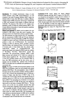
CHAOS
VOLUME 14, NUMBER 3
SEPTEMBER 2004
Pattern dynamics in a checkerboard map
N. J. Balmforth
Departments of Mathematics and Earth and Ocean Science, University of British Columbia, Vancouver,
British Columbia V6T 1Z2, Canada
E. A. Spiegela)
Department of Astronomy, Columbia University, New York, New York 10027
共Received 8 April 2004; accepted 1 July 2004; published online 16 September 2004兲
Differential equations often have solutions in the forms of trains of coherent structures such as
pulses and antipulses. For such sytems, the methods of singular perturbation theory permit the
derivation of pattern maps that predict the sequence of spacings between successive pulses. Here we
apply such a procedure to cases where two distinct kinds of pulse 共or antipulse兲 may coexist in the
system. In that case, direct application of the method leads to multivalued maps that make for
complicated descriptions, especially when the succession of pulse types becomes chaotic. We show
how this description may be simplified by using maps arrayed in checkerboard style to provide
causal descriptions of both the successions of pulse spacings and the order in which the different
kinds of pulse go by. © 2004 American Institute of Physics. 关DOI: 10.1063/1.1784752兴
grounds such as dimensional arguments and, for this reason,
they are called coherent structures. The earliest studies of
such objects were made in the context of conservative systems as in relativity1 and quantum field theory.2 In those
subjects, the coherent structures are likened to material particles whose dynamics may be described by equations of
motion derived from the underlying field theory. Such reductions are desirable when more than one coherent structure
arises, for then the objects interact and the subsequent evolution becomes difficult to analyze in the field theory. Similar
approaches have been developed for the study of coherent
structures in dissipative field theories, both for pulses and
kinks.3–9
One reason for raising the distinction between the conservative and the dissipative field theories lies in a comparison of the corresponding kinds of dynamical system. In the
conservative case, a periodic orbit will retain any energy it is
assigned; in dissipative systems, the stable periodic orbits are
the more rigidly prescribed limit cycles. This distinction between the two cases carries over to the spatial structures so
that, in the dissipative case, the derived equations of motion
tend to be more constraining.
Our discussion here concerns an aspect of the derivation
of equations of motion for the coherent structures that appear
in the study of dissipative nonlinear partial differential equations in one space dimension only and in time. When only
one kind of coherent structure is admitted, the derivation of
approximate equations of motion by asymptotic means has
been thoroughly documented in the references just cited. We
shall briefly sketch the general approach for this case in Sec.
I B as a prelude to a discussion of the feature of this problem
that is of particular interest to us in this study. Accordingly,
we consider situations in which two different kinds of coherent structure enter the dynamics. We confine attention here to
the simplest case in which there exists a reference frame in
which the resulting pulse train is steady. The pattern theory
that then arises involves multivalued maps and our aim is to
Dissipative systems of differential equations exhibit the
same kind of wave particle duality that one sees in conservative systems. Here, by particle, we mean a long-lived
solitary wave that emerges as a simple nonlinear solution
of the basic equations. When several of such discrete objects form, it becomes difficult to solve the nonlinear partial differential equations that spawn them. Instead, one
may discretize the system by reducing it to equations of
motion for the solitary structures, allowing for their interactions. This reduction is quite effective as long as the
structures remain widely separated. In that case the tidal
distortions are small and perturbative procedures are
quite accurate. So that this approach should lead to finite
results, we must impose a condition that is a standard of
this kind of procedure—called singular perturbation
theory—to ensure that it leads directly to finite results.
However, when the system admits more than one kind of
solitary wave, those results are unwieldy. Hence the aim
of the present work is to describe a simplifying procedure
that renders the results manageable and leads to rules
that predict both the successive spacings of the solitary
structures and the succession of wave types in a given
train of them. To keep the presentation relatively brief,
we study only the case where there exists a frame of motion in which the spacings of the structures remain constant in time, but we indicate briefly how a more general
approach may be formulated.
I. INTRODUCTION
A. Statement of the problem
Many nonlinear field theories yield solutions in the form
of localized structures or solitary waves. These typically exist for longer times than might be anticipated on naive
a兲
Electronic mail: [email protected]
1054-1500/2004/14(3)/784/9/$22.00
784
© 2004 American Institute of Physics
Downloaded 05 Oct 2004 to 137.82.36.23. Redistribution subject to AIP license or copyright, see http://chaos.aip.org/chaos/copyright.jsp
Chaos, Vol. 14, No. 3, 2004
Pattern dynamics in a map
show how to rearrange these results into checkerboards of
maps of the interval.10 These are single-valued maps of a
composite interval that carry information on the nature of the
successive pulses as well as on their spacing.
B. Sketch of the method
Let u(x,t) be a set of scalar fields in a two-dimensional
space–time (x,t). Suppose that we are given field equations
in the form
⳵ t u⫽Lp共 ⳵ x 兲 u⫹N共 u兲 .
共1.1兲
Here Lp is a linear differential operator that depends on parameters p and N is a strictly nonlinear operator that may
similarly contain spatial derivatives and parameters. We assume that 兩u兩 goes rapidly to zero as 兩 x 兩 goes to ⫾⬁. There
is no explicit time dependence in either operator.
We first assume the existence of a solitary solution of the
equation that is steady in a frame moving in x at speed c.
Such a solution has the form
u共 x,t 兲 ⫽U共 ␹ 兲
for
␹ ⫽x⫺ct.
共1.2兲
When we introduce Eq. 共1.2兲 into Eq. 共1.1兲, we obtain the
ordinary differential equation
Lp共 D 兲 U⫹cDU⫹N共 U兲 ⫽0.
共1.3兲
In the far wings of the solitary structure, 兩U兩 is quite small
and we may linearize the equation in those regions; that is,
we linearize about the state U⫽0. The equation is constructed so that linearization is achieved by dropping the
term N共U兲. The linearized equation admits solutions whose
␹-dependence is like exp关(␴⫹i␻)␹兴. We consider only the
simple case where for suitable parameter values there are just
two eigenvalues 共if we count a complex conjugate pair as a
single eigenvalue兲 with the property that one of the roots 共or
pairs兲 has positive real part and the other has negative real
part. Thus one solution decays in the positive ␹ direction and
the other in the negative ␹ direction. Then we may further
seek conditions in which the two linear solutions form the
wings of one or more types of pulsatile solutions, when we
regard ␹ as analogous to time in a dynamical system. There
is a great range of possible types of such homoclinic solutions distinguished in particular by the number of times they
wind around the various fixed points of the system. We shall
work with only a very few of the simplest forms of these and
merely cite two attempts to classify some of the
possibilities.11,12
Finding a homoclinic solution involves a determination
of the parameters for which it may exist. If we specify parameter values p0 , we need then to find the values of c(p0 )
for which one or, as in the following, more such solutions
exist. The simplest and most studied situation is the one in
which, for given p0 , there is only one homoclinic solution
共or pulse兲 U⫽H( ␹ ) with its maximum value placed arbitrarily at ␹ ⫽0. When ␧⫽ 兩 p⫺p0 兩 is sufficiently small, numerical solutions to the problem typically take the form of a
series of widely separated, propagating pulses. Then we may
look for approximate solutions in the form of series of pulses
whose separations become larger as ␧ gets smaller. This form
of solution may be written 共in the case of N pulses兲 as
785
N
u共 x,t 兲 ⫽
兺
k⫽1
H共 ␹ ⫺ ␹ k 兲 ⫹␧R共 ␹ , 兵 ␹ k 其 ,␧ 兲 ,
共1.4兲
where ␧R is the error made in assuming that a linear superposition of coherent structures approximates a nonlinear solution.
As part of the approximation, we let R depend on ␹ and
on the set of instantaneous positions 兵 ␹ k 其 at which the pulses
are found in the moving frame. The idea is then to keep the
error small by requiring R to be finite through a solvability
condition arising in the asymptotic development. This condition fixes the ␹ k in the special case where the spacings are
stationary in some appropriate frame. The situation is then
the same if the original problem is posed as an ordinary
differential equation and ␹ is actually the time. Then the
same sort of approximation may be introduced and the development based on Eq. 共1.4兲 leads to maps of the pulse
spacings equivalent to those found using the arguments of
Shilnikov.12,13 However, for partial differential equations, the
initial conditions will typically involve a set of ␹ k that do not
accord with the results of this map. To deal with this feature
of the solutions, we may let ␹ k be a function of ␧t. Then the
solvability condition leads instead to equations of motion for
the pulses, seen as particles. These equations typically allow
the pulses to relax into fixed spacing 共in a suitable frame兲
that do accord with the spacing map, though we have no
proof that this relaxation always takes place.
When more than one kind of pulse enters the dynamics,
we may seek equations of motion for them. In our experience, pulse trains tend to lock into fixed spacings. So, to
keep our discussion of this more complicated case as simple
as possible, we assume that the pulse train has already locked
into a solution that is steady in the appropriate moving
frame. Thus we are really treating only the ODE 共1.3兲. The
maps for this steady case generally are multivalued, as it will
turn out, and we describe how to deal with this inconvenience by introducing arrays of interval maps that have been
called checkerboard maps.10 A clue to the way to do this
comes from the case where a pulse and its mirror image enter
the problem.12,14 We shall proceed in an illustrative example
that we describe next.
C. The example
To illustrate the problem of multiple pulse types, we turn
to the general equation for the dynamics of waves in thin
films.15–17 This is an asymptotic description of twodimensional flow in a thin liquid film with horizontal velocity u(x,t) given by
⳵ t u⫹u ⳵ x u⫹ ␬ u 2 ⳵ x u⫽ ␰⳵ 2x u⫹ ␩ ⳵ 3x u⫹ ␨⳵ 4x u,
共1.5兲
where ␰, ␩, ␨, and ␬ are constants. When we look for solutions in the form 共1.2兲, we are led to the ordinary differential
equation
d 2 U dU
d 3U
⫹
⫺ ␤ U⫹ ␣ U 2 ⫹U 3 ⫽0,
3 ⫹␮
d␹
d␹2 d␹
共1.6兲
where the variables have been scaled so that there are only
three control parameters, ␣, ␤, and ␮, as indicated. This
Downloaded 05 Oct 2004 to 137.82.36.23. Redistribution subject to AIP license or copyright, see http://chaos.aip.org/chaos/copyright.jsp
786
Chaos, Vol. 14, No. 3, 2004
N. J. Balmforth and E. A. Spiegel
FIG. 1. 共Color online兲 Pulse and antipulse solutions to Eq. 共1.3兲. Inset panels show phase portraits projected onto
the (U,U̇) plane. Panel 共a兲 shows a
case with symmetry ( ␣ ⫽0,␮ ⫽0.7,
␤ ⫽1.107 887). Panel 共b兲 shows a
case in which the pulse has a single
primary peak, but the antipulse has
two peaks ( ␣ ⫽⫺3.672, ␮ ⫽0.816 45,
␤ ⫽0.852 806).
ODE is a particular case of a model equation from the study
of convection with competing instabilities.18,19 The examples
with either the ultimate or the penultimate term on the left
omitted have been studied in some detail.19–21 Partial differential equations whose traveling waves are described by an
ODE of the same genre arise in several disciplines.22–24 As
we already mentioned, we may think of Eq. 共1.6兲 as a dynamical system with ␹ playing a role analogous to time. We
shall study choices of the parameters where the solutions of
Eq. 共1.6兲 are trains of widely separated solitary structures
that may be of different types.
II. EXPANSIONS IN PULSES
A. Homoclinic orbits
Equation 共1.6兲 has three fixed points when ␹ is considered as a time:
U⫽0,
U⫽U ⫾ ⫽ 21 共 ⫾ 冑␣ 2 ⫹4 ␤ ⫺ ␣ 兲 .
共2.1兲
Each of these organizes the flow in particular regions of the
phase space (Ü,U̇,U), but we concentrate on parameter regimes in which the dominant features of the solutions are
homoclinic orbits issuing from the origin. These are the orbits that asymptote to the origin as ␹ →⫾⬁. Even this restricted class of orbits has many variants, but we shall be
concerned with only those orbits that, having emerged from
the origin, then encircle one of the other fixed points U ⫾
only once or twice before returning back to the origin. The
orbits looping around the positive fixed point U ⫹ have predominantly positive amplitude, and we refer to them as
pulses; those that encircle U ⫺ and traverse mainly the region
U⬍0 of phase space are the antipulses; examples are shown
in Fig. 1.
Such coherent structures can be found when the parameter values lie in certain surfaces in parameter space given by
a condition of the form
␮⫽␮共 ␣,␤ 兲.
共2.2兲
These conditions define what we call the homoclinic loci.12
B. The expansion
For parameter values very near to a homoclinic locus
given by Eq. 共2.2兲, there are solutions that take the form of
trains of widely spaced pulses, as one sees with a little nu-
merical exploration. Since we are interested in deriving approximate solutions containing a mixture of pulses and antipulses, we choose the value of ␮ to bring us close to values
␣ ⫽ ␣ 0 and ␤ ⫽ ␤ 0 for which a pulse and antipulse coexist.
Then we develop around this special condition using the
small parameter ␧ and write
␣ ⫽ ␣ 0 ⫹␧ ␣ 1 ,
␤ ⫽ ␤ 0 ⫹␧ ␤ 1 .
共2.3兲
For the development to be meaningful, we need to assume
that the amplitudes of the overlapping portions of individual
structures are O(␧). If their separations are much smaller
than this condition allows, we cannot reliably distinguish the
pulses. For extremely large separations, we basically see isolated structures. Moreover, a large enough separation leaves
open regions that may be unstable to the formation of new
pulses; this raises an issue that needs special treatment.25
As a measure of the size of the typical pulse separation,
L, we choose
␧⫽e ⫺L ␴ ,
共2.4兲
⫺1
where ␴ is a characteristic decay length fore and aft. With
␧ as the small parameter 共or L a large one兲, we take the other
parameters, 共␮, ␣ 1 , and ␤ 1 ) to be of order unity.
With ␧ small, we are in the nearly homoclinic conditions
that obtain close to ( ␣ 0 , ␤ 0 ). We designate a single homoclinic structure as H( ␹ ; ␽ ), where the phase of ␹ is chosen so that the extreme is at zero argument and the parameter
␽ identifies the nature of the pulse, as explained in the following. In a series of N pulses, we approximate the kth one
as H k ⫽H( ␹ ⫺ ␹ k ; ␽ k ) where the sequence of pulses is ordered so that ␹ k⫹1 ⬎ ␹ k .
The slight generalization of Eq. 共1.4兲 for more than one
kind of solitary structure that we need as an approximate
solution to Eq. 共1.3兲 is
N
u⫽
兺
k⫽1
H k ⫹␧R共 ␹ , 兵 ␹ m 其 , 兵 ␽ k 其 ,␧ 兲 ,
共2.5兲
where ␧R is the error made in assuming a solution in the
form of a linear superposition. Near the core of a particular
pulse, the error in its neighborhood comes mainly from the
tails of the nearest neighbors and this has been tuned to be
O(␧). When we insert this ansatz into Eq. 共1.3兲 we recover
in leading order the fact that a single pulse is a solution of
the basic equation. Thus
Downloaded 05 Oct 2004 to 137.82.36.23. Redistribution subject to AIP license or copyright, see http://chaos.aip.org/chaos/copyright.jsp
Chaos, Vol. 14, No. 3, 2004
Pattern dynamics in a map
787
FIG. 2. 共Color online兲 Spacing functions, F jk (⌬), corresponding to the
homoclinic orbits shown in Fig. 1. In
共a兲, the pulse and antipulse are mirror
images and F ↑↑ (⌬)⫽F ↓↓ (⌬)⬅F(⌬)
⬅⫺F ↑↓ (⌬)⫽⫺F ↓↑ (⌬). The ‘‘duplication’’ function is F(⌬); the ‘‘flip’’
function is ⫺F(⌬). In 共b兲, there is no
such symmetry; the functions F ↓↑ and
F ↓↓ are offset for clarity.
冉
冊
d3
d2
d
⫹
⫺ ␤ 0 H k ⫹H 3k ⫹ ␣ 0 H 2k ⫽0.
2 ⫹␮
d␹
d␹2 d␹
共2.6兲
The nearest neighbors to this pulse are each O(␧) in
amplitude for ␹ near ␹ k while those beyond are even smaller
in that neighborhood. Hence the interaction between nearest
neighbors is strongest and it enters at order ␧. The terms of
order ␧ give
Lk R⫽ ␤ 1 H k ⫹ ␣ 1 H 2k ⫺
where
冉
3
1
f 共 H k 兲关 H k⫹1 ⫹H k⫺1 兴 ,
␧
冊
2
d
d
d
⫹␮ 2 ⫹
⫺␤0 ⫹ f 共 Hk兲,
Lk ⫽
d␹2
d␹
d␹
共2.7兲
1
␧I k
F k, j 共 ⌬ 兲 ⫽
冕
⬁
⫺⬁
N k 共 ␹ 兲 f 关 H k 共 ␹ 兲兴 H j 共 ␹ ⫹⌬ 兲 d ␹ , 共2.11兲
where
I k⫽
共2.8a兲
and
冕
⬁
⫺⬁
N k 共 ␹ 兲 H k 共 ␹ 兲 dx,
f 共 H 兲 ⫽3H ⫹2 ␣ 0 H .
共2.8b兲
2
Since H k⫾1 is O(␧) near ␹ k , the last term on the right of Eq.
共2.7兲 is O(1).
To ensure that the error term in Eq. 共2.5兲 is O(␧), we
require that R be finite. We therefore impose the condition
that the solution of Eq. 共2.7兲 should be soluble in finite
terms. For this, the inhomogeneous term on the right of Eq.
共2.7兲 must be orthogonal to the null vector of L †k , the adjoint
of Lk . To define the adjoint, we adopt integration in ␹ from
⫺⬁ to ⫹⬁ as the inner product in the space of functions
which vanish for ␹ →⫾⬁. We find that the adjoint operator
is
冉
冊
d2
d3
d
L †k ⫽ ⫺ 3 ⫹ ␮ 2 ⫺ ⫺ ␤ 0 ⫹ f 共 H k 兲 .
d␹
d␹
dx
共2.9兲
The existence of null vectors, N k ⫽N( ␹ ⫺ ␹ k , ␽ k ), of the adjoint operator has been demonstrated by L. N. Howard 共personal communication兲 and they are not hard to compute numerically. Then, the condition that the right-hand side of Eq.
共2.7兲 should be orthogonal to these null vectors is
冕
⬁
⫺⬁
N kH kd ␹ ⫺ ␣ 1
1
⫽
␧
冕
⬁
⫺⬁
冕
⬁
⫺⬁
N k H 2k d ␹
N k f 共 H k 兲关 H k⫹1 ⫹H k⫺1 兴 d ␹ .
共2.12兲
Eq. 共2.10兲 becomes the return map,
␤ 1 ⫺S k ⫽F k,k⫹1 共 ⫺⌬ k⫹1 兲 ⫹F k,k⫺1 共 ⌬ k 兲 ,
2
␤1
This condition controls the spacings of the sequence of
pulses and it is a generalization of previous versions in
which all the pulses are alike or are mirror images of each
other.12,14
We let ⌬ k ⫽ ␹ k ⫺ ␹ k⫺1 and write H k⫹1 ⫽H( ␹ ⫺ ␹ k
⫹⌬ k⫹1 , ␽ k⫹1 ). If we define the function F k, j (⌬) by the
relation
共2.13兲
with
S k⫽
␣1
␧I k
冕
⬁
⫺⬁
N k 共 ␹ 兲 H 2k 共 ␹ 兲 d ␹ .
共2.14兲
Sample spacing functions, F jk (⌬), are shown in Fig. 2. The
functions possess structure near the core of the pulse, but
decay exponentially to the right and left; in the examples
shown, the functions decay with oscillations to the right.
C. Spacing and polarity maps
Condition 共2.13兲 determines the spacing, ⌬ k⫹1 , given
⌬ k and the polarities of the previous two pulses. In fact, the
relation gives more than this since it also determines the
polarity of (k⫹1)st pulse, as we shall illustrate once we
have introduced some notation.
To represent polarity, we set ␽ k ⫽1 if the kth object is a
pulse, and ␽ k ⫽⫺1 if it is an antipulse. The dependencies of
the function F j,k are then written more transparently as
F j,k 共 ⌬ 兲 ⫽F 共 ⌬; ␽ k , ␽ j 兲 ,
共2.15兲
and the spacing map as
共2.10兲
C 1 共 ␽ k 兲 ⫽F 共 ⫺⌬ k⫹1 ; ␽ k , ␽ k⫹1 兲 ⫹F 共 ⌬ k ; ␽ k , ␽ k⫺1 兲 ,
共2.16兲
where
Downloaded 05 Oct 2004 to 137.82.36.23. Redistribution subject to AIP license or copyright, see http://chaos.aip.org/chaos/copyright.jsp
788
Chaos, Vol. 14, No. 3, 2004
C 1 共 ␽ k 兲 ⫽ ␤ 1 ⫺S 共 ␽ k 兲 .
N. J. Balmforth and E. A. Spiegel
共2.17兲
III. EXAMPLES
A. The antisymmetric case
To streamline the formulas even further in considering specifically pulses or antipulses, we replace the ␽ k arguments
with the subscripts, ↑ and ↓, for ␽ ⫽⫾1.
Our task is now to make sense of Eq. 共2.16兲, which is to
be solved for ⌬ k⫹1 and ␽ k⫹1 , knowing ⌬ k , ␽ k⫺1 , and ␽ k
from the previous pair. If a pulse train begins with a succession of pulses, then the spacing map is simply
F ↑↑ 共 ⫺⌬ k⫹1 兲 ⫽C 1,↑ ⫺F ↑↑ 共 ⌬ k 兲 .
共2.18兲
As long as one can invert F ↑↑ (⫺⌬ k⫹1 ), the pulse train continues indefinitely. However, F ↑↑ (⫺⌬ k⫹1 ) can be inverted
only when C 1,↑ ⫺F ↑↑ (⌬ k ) is positive since F ↑↑ (⌬) returns a
positive value for sufficiently large and negative argument
共see Fig. 2兲. Consequently, when C 1,↑ ⫺F ↑↑ (⌬ k ) becomes
negative 共and this does happen兲, the continuation fails. This
noninvertibility does not signal a breakdown of the
asymptotic theory. It is simply what happens at a switch of
polarity when the trajectory in phase space finds it way
around the stable manifold into the origin and enters the
region where U⬍0. Then the trajectory follows a path close
to the homoclinic orbit lying chiefly in U⬍0 to create an
antipulse. Thus, a terminating iteration of Eq. 共2.18兲 indicates a polarity reversal and the subsequent map is
F ↑↓ 共 ⫺⌬ k⫹2 兲 ⫽C 1,↑ ⫺F ↑↑ 共 ⌬ k⫹1 兲 .
共2.19兲
Since F ↑↓ has negative amplitude, Eq. 共2.19兲 can be inverted
for ⌬ k⫹2 when the pulses are well spaced 共see Fig. 2兲.
Immediately after this reversal, the polarity either flips
again, signifying a return to a pulse, or remains negative and
antipulse follows antipulse. Those transitions are described
by the conditions,
冎
F ↓↑ 共 ⫺⌬ k⫹3 兲
or
⫽C 1,↓ ⫺F ↓↑ 共 ⌬ k⫹2 兲 ,
F ↓↓ 共 ⫺⌬ k⫹3 兲
For the antisymmetric case, ␣ ⫽0, pulses and antipulses
are mirror images and are identical up to a sign—the polarity, ␽ k 关see Fig. 1共a兲兴. This sign factors out of the various
integrals in the spacing functions; also S k ⫽0. The solvability
condition 共2.13兲 can be written as12,14
␤ 1 ⫽⌰ k⫹1 F 共 ⫺⌬ k⫹1 兲 ⫹⌰ k F 共 ⌬ k 兲 ,
共3.1兲
where ⌰ k ⫽ ␽ k ␽ k⫺1 is a relative-polarity parameter, and
F(⌬) is simply 兩 F(⌬, ␽ j , ␽ k ) 兩关see Fig. 2共a兲兴. Because ⌰ k
takes either sign, we get a two-branched map of the interval,
⌬, examples of which are given in Ref. 13. With
Zk ⫽F 共 ⫺⌬ k 兲 ,
共3.2兲
the map becomes
⌰ k⫹1 Zk⫹1 ⫽ ␤ 1 ⫺⌰ k F共 Zk 兲 ,
共3.3兲
⫺1
where F(Z)⫽F 关 ⫺F (Z) 兴 . The duplicity of the map is
removed by expressing the spacing relations as a continuous
map in the ⌰ k Zk ⫺⌰ k⫹1 Zk⫹1 plane. The signs of ⌰ k can
then be absorbed into the definition of Zk , and the map
becomes
Zk⫹1 ⫽
再
␤ 1 ⫺F共 Zk 兲
in Zk ⬎0
␤ 1 ⫹F共 Zk 兲
in Zk ⬍0.
共3.4兲
To this order in the development in ␧, this map is singlevalued. Second-order corrections to the map in the
asymptotic theory do introduce multivaluedness at order ␧
through the entry of next-nearest neighbors into the interactions. Yet higher-order corrections introduce even more multivaluedness, in keeping with the expected underlying Cantorial structure.12
B. Weak asymmetry
共2.20兲
respectively. Which of these options one takes is determined
by the sign of the right-hand side.
In summary, we iterate Eq. 共2.16兲 by choosing the polarity of the (k⫹1)st pulse according to the sign of the discriminant C 1 ( ␽ k )⫺F(⌬ k ; ␽ k , ␽ k⫺1 ), and then determining
the next spacing by inverting the 共now invertible兲 function
F k,k⫹1 (⫺⌬ k⫹1 ). In the case where the train consists entirely
of pulses, this procedure would be the same as has been used
when only one kind of solitary object enters the dynamics
and it would lead to a one-dimensional spacing map. For the
more complicated problem we face here, we try to use the
same kind of approach by using sequences of such simple
maps. However, since there are four possible realizations of
C 1 ( ␽ k )⫺F(⌬ k ; ␽ k , ␽ k⫺1 ), there are four branches of the
map. The transition rules between the branches are dictated
by the polarities of the current pair of pulses. We shall illustrate this complicated structure in the following, though a
quick peek at Fig. 4 at this point might suggest the kind of
structure we are describing.
We next weakly break the symmetry between the pulses
and antipulses by reintroducing the term ␣ U, 2 but with ␣
⫽␧. In the numerical example illustrated in Fig. 3, the first
panel shows U( ␹ ), and the second panel shows a phase portrait projected onto the (U,U̇) plane. The sequence of pulse
spacings and polarities extracted from a much longer time
series is shown against k in the third and fourth panels.
At leading order, the homoclinic solutions are again
symmetrical. That is, an antipulse solution is ⫺H( ␹ ⫺ ␹ k )
⫹O(␧) so that the structural differences between pulse and
antipulse are delayed to order ␧ and enter only into R.
Hence, just as in Eq. 共3.1兲 of the antisymmetric case, we
have that
F 共 ⌬, ␽ j , ␽ k 兲 ⫽ ␽ j ␽ k F 共 ⌬ 兲 .
共3.5兲
If we proceed as described in the discussion following
Eq. 共2.20兲, we are led to the four-branched map of the pulse
spacings, ⌬ k , shown in Fig. 4. This picture compares spacings extracted from the solution of Fig. 3 with the predictions
of Eq. 共2.13兲, using the spacing functions illustrated in Fig.
2. As a test of accuracy of the asymptotics it is useful, but
such a map is too unwieldy and we must simplify things.
Downloaded 05 Oct 2004 to 137.82.36.23. Redistribution subject to AIP license or copyright, see http://chaos.aip.org/chaos/copyright.jsp
Chaos, Vol. 14, No. 3, 2004
Pattern dynamics in a map
789
FIG. 3. A numerical solution of Eq.
共1.3兲 with ␮ ⫽0.7, ␣ ⫽0.01, and ␤
⫽1.108. The first panel shows a time
series of U(t). The second panels
show a phase portrait projected on to
the (U,U̇) plane. The solution is
barely distinguishable from the nearby
homoclinic orbits, and consequently
the portrait looks little different from
the inset of Fig. 1共a兲. A sequence of
pulse spacings (⌬ k ) and polarities
( ␽ k ) taken from a much longer time
series is shown in the third and fourth
panels 共as points connected by dotted
lines兲.
Again, we introduce ⌰ k ⫽ ␽ k ␽ k⫺1 , then proceed as for
the symmetric case by considering the ⌰ k Zk plane, absorbing the signs into Zk defined in Eq. 共3.2兲. An important difference, however, is that S k is no longer equal for pulses and
antipulses, since
Zk⫹1 ⫽
再
C 1 ⫹⌬C⫺F共 Zk 兲
in Z⬎0
C 1 ⫹⌬C⫹F共 Zk 兲
in Z⬍0,
共3.8兲
or
with C 1 ⫽ ␤ 1 ⫹S and ⌬C⫽⫺2S. (⌬C measures the separation of the pulse and antipulse homoclinics at ␣ ⫽␧ ␣ 1 .)
Which branch one iterates depends on the polarity of the two
pulses under consideration.
Thus, as a consequence of symmetry breaking, the Zk
map develops two irreducible branches. This is illustrated in
Fig. 5. On transformation to the ⌰ k Zk plane, two of the
curves of the equivalent spacing map move into ⌰ k Zk ⬍0
and these correspond to flip maps 共Fig. 5兲. The two unchanged branches are duplication maps for pulses and anti-
FIG. 4. The spacing map constructed from the solution shown in Fig. 3. The
points show the measured spacings, whereas the curves show the fourvalued map predicted by perturbation theory 关i.e., Eq. 共2.13兲兴. The dotted
lines show a sample iteration 共the diagonal is also shown兲.
FIG. 5. The ⌰ k Zk map constructed from the solution of Fig. 3. Dots again
show measured spacings, converted into values for Zk using Eq. 共3.2兲 and
the spacing functions shown in Fig. 2. The solid curves display the doublevalued map predicted by asymptotics.
S k ⫽ ␽ k S.
共3.6兲
Therefore, instead of a single relation like Eq. 共3.4兲, we obtain the two-branched map,
Zk⫹1 ⫽
再
C 1 ⫺F共 Zk 兲
in Z⬎0
C 1 ⫹F共 Zk 兲
in Z⬍0,
共3.7兲
Downloaded 05 Oct 2004 to 137.82.36.23. Redistribution subject to AIP license or copyright, see http://chaos.aip.org/chaos/copyright.jsp
790
Chaos, Vol. 14, No. 3, 2004
N. J. Balmforth and E. A. Spiegel
a doubly peaked antipulse; Fig. 1共b兲 displays the relevant
homoclinic orbits, and Fig. 2共b兲 the spacing functions constructed from them. Figure 7 shows a sample solution nearby
in parameter space; the corresponding four-valued spacing
map appears in Fig. 8. The map 共2.13兲 cannot be simplified
any further in this example, but its multiplicity can still be
reduced by first reformulating in terms of ⌰ k Zk 共Fig. 9兲,
where Zk ⫽F ↓↓ (⫺⌬ k ) and then checker-boarding 共Fig. 10兲.
Again, the agreement with the direct numerical results is
very good.
IV. DISCUSSION
FIG. 6. A single-valued map obtained from the Zk map shown in Fig. 5 by
breaking the curves into four pieces and placing them into the squares of a
checkerboard. Points show measurements and curves indicate the
asymptotic theory.
pulses. The remaining twofold multiplicity is removable because the multibranched map can be seen as a onedimensional map with additional transition rules between
each branch. We can construct a checkerboard map10 from
this by breaking apart the four pieces and placing them in a
four-square checker board as illustrated in Fig. 6. The location of the pieces within the sixteen boxes follows from the
transition rules. It is straightforward to verify that the checkerboard correctly represents the dynamics of the twobranched map.
C. Strong asymmetry
As a final example, we consider an asymmetry so extreme that a pulse with a single dominant peak coexists with
When the solution of differential equations takes the
form of a train of pulses that are all nearly alike, it is possible
to represent this outcome by an expansion in terms of fundamental structures. In this picture, the pulses in the sequence differ slightly from one another because of their interactions. The approach is different from another expansion
that uses 共slightly兲 differing periodic orbits, though there is
perhaps some commonality between the two visions. What
we have studied here is the extension of the pulse expansions
to cases where there are two different kinds of pulses that
may enter into the dynamics. This is still a far cry from the
case where there is a continuum of pulse types, but we hope
that it may be a good beginning.
We have simplified our treatment to finding the rules for
successive spacing and kinds of pulses for only a steadily 共in
some frame兲 propagating train, but the extension to slowly
varying positions is not difficult, as we know from the cited
earlier work with one kind of pulse. But there are more generalizations that call for attention.
The restriction to one-dimensional cases with few symmetries leads one to hope that more can be done. What we
have looked at here is the extension to the situation where
two kinds of objects can interact. The generalization to cases
where there are even more kinds of objects, but of a discrete
number, looks tractable with additional squares in the checkerboard.
A more difficult issue is that we have studied only cases
where the number of pulses in the solution is specified in
FIG. 7. A numerical solution of Eq.
共1.3兲 with ␮ ⫽0.816 45, ␣ ⫽⫺3.672,
and ␤ ⫽0.852 806. Panels as in Fig. 3.
Downloaded 05 Oct 2004 to 137.82.36.23. Redistribution subject to AIP license or copyright, see http://chaos.aip.org/chaos/copyright.jsp
Chaos, Vol. 14, No. 3, 2004
Pattern dynamics in a map
FIG. 8. A similar picture to Fig. 4, but showing the spacing map for the
solution of Fig. 7.
advance. Is there a way to allow this number to change in the
course of the dynamics? One way to broach this question
might be to introduce an analogue of creation and destruction
operators for dissipative systems. It is unclear at this time
whether such a notion can be made meaningful but a good
starting point might be the nearly integrable case that has
been studied in some detail.26
The inclusion of further group parameters besides position is of interest as well, especially of the amplitude itself
when this characteristic is a continuous variable. Also the
problem of higher dimensional objects poses some interest-
791
FIG. 10. The single-valued checkerboard map corresponding to Fig. 9.
ing difficulties,27 particularly in the issue of the interactions
of the structures. These are the kinds of questions that the
earliest workers grappled with and they are still pretty much
open. We hope for more news at the next significant birthdays of our dedicatees.
For now, we must rest our case with the final observation
that the asymptotic methods used in this problem appear to
provide remarkable accuracy and, on those grounds alone,
have proved their worth. One reason that there has been no
discernible difference between the numerical and the
asymptotic solutions is probably that the asymptotics does
not seem to lead to small pulse spacings, though these are
allowed by the procedure. No doubt it would be best in
asymptotic studies to rule out cases with small pulse separations, for these are outside the domain of validity of the pulse
expansions 共this was our basic premise in ignoring the ambiguities at small spacing when inverting the space function
F兲. However, as yet, we have seen no problems arising from
this aspect of the work.
1
FIG. 9. A similar picture to Fig. 5, but showing the Zk map for the solution
of Fig. 7.
A. Einstein, L. Infeld, and B. Hoffman, ‘‘The gravitational equations and
the problem of motion,’’ Ann. Math. 39, 65–110 共1938兲.
2
P. Cvitanovic, Field Theory 共Nordita Lecture Notes, Copenhagen, 1983兲.
3
J.R. Keener and D.W. McLaughlin, ‘‘Solitons under perturbation,’’ Phys.
Rev. A 16, 777–785 共1977兲.
4
K.A. Gorshkov and L.A. Ostrovsky, ‘‘Interactions of solitons in nonintegrable systems: Direct perturbation method and applications,’’ Physica D
3, 428 – 438 共1981兲.
5
K. Kawasaki and T. Ohta, ‘‘Kink dynamics in one-dimensional nonlinear
systems,’’ Physica A 116, 573–593 共1982兲.
6
P. Coullet, C. Elphick, and D. Repaux, ‘‘Nature of spatial chaos,’’ Phys.
Rev. Lett. 58, 431– 438 共1987兲.
7
C. Elphick, E. Meron, and E.A. Spiegel, ‘‘Patterns of propagating pulses,’’
SIAM 共Soc. Ind. Appl. Math.兲 J. Appl. Math. 50, 490–503 共1990兲.
8
N.J. Balmforth, ‘‘Coherent structures and homoclinic orbits,’’ Annu. Rev.
Fluid Mech. 27, 335–355 共1995兲.
9
N.J. Balmforth, G.R. Ierley, and R. Worthing, ‘‘Pulse dynamics in an
unstable medium,’’ SIAM 共Soc. Ind. Appl. Math.兲 J. Appl. Math. 56, 205–
225 共1997兲.
Downloaded 05 Oct 2004 to 137.82.36.23. Redistribution subject to AIP license or copyright, see http://chaos.aip.org/chaos/copyright.jsp
792
10
Chaos, Vol. 14, No. 3, 2004
N.J. Balmforth, E.A. Spiegel, and C. Tresser, ‘‘Checkerboard maps,’’
Chaos 5, 216 –226 共1995兲.
11
H.-C. Chang, E.A. Demekhin, and D.I. Kopelevich, ‘‘Laminarizing effects
of dispersion in an active-dissipative nonlinear medium,’’ Physica D 63,
299–320 共1993兲.
12
N.J. Balmforth, G.R. Ierley, and E.A. Spiegel, ‘‘Chaotic pulse trains,’’
SIAM 共Soc. Ind. Appl. Math.兲 J. Appl. Math. 54, 1291–1234 共1994兲.
13
P. Coullet and C. Elphick, ‘‘Topological defect dynamics and Melnikov’s
theory,’’ Phys. Lett. A 121, 233–236 共1987兲.
14
P. Glendinning, ‘‘Bifurcations near homoclinic orbits with symmetry,’’
Phys. Lett. A 103, 163–166 共1984兲.
15
D.J. Benney, ‘‘Long waves on liquid films,’’ J. Math. Phys. 共Cambridge,
Mass.兲 45, 150–155 共1966兲.
16
G.M. Homsy, ‘‘Model equations for wavy viscous film flow,’’ Lect. Appl.
Math. 15, 191–194 共1974兲.
17
B.S. Tilley, S.H. Davis, and S.G. Bankoff, ‘‘Nonlinear long-wave stability
of superposed fluids in an inclined channel,’’ J. Fluid Mech. 277, 55– 83
共1994兲.
18
D.W. Moore and E.A. Spiegel, ‘‘A thermally excited nonlinear oscillator,’’
Astrophys. J. 143, 871 共1966兲.
19
A. Arneodo, P.H. Coullet, and E.A. Spiegel, ‘‘Dynamics of triple convec-
N. J. Balmforth and E. A. Spiegel
tion,’’ Geophys. Astrophys. Fluid Dyn. 31, 1– 48 共1985兲.
A. Arneodo, P.H. Coullet, E.A. Spiegel, and C. Tresser, ‘‘Asymptotic
chaos,’’ Physica D 14, 327–347 共1985兲.
21
P. Glendinning and C. Sparrow, ‘‘Local and global behaviour near homoclinic orbits,’’ J. Stat. Phys. 35, 645– 696 共1984兲.
22
V. Degiorgio, R. Piazza, M. Corti, and C. Minero, ‘‘Critical properties of
nonionic micellar solutions,’’ J. Chem. Phys. 82, 1025 共1985兲.
23
C. Elphick, E. Meron, J. Rinzel, and E.A. Spiegel, ‘‘Impulse patterning
and relaxational propagation in excitable media,’’ J. Theor. Biol. 146,
249–268 共1990兲.
24
K.B. Glasner and T.P. Witelski, ‘‘Coarsening dynamics of dewetting
films,’’ Phys. Rev. E 67, 016302 共2003兲.
25
S. Toh and T. Kawahara, ‘‘On the stability of soliton-like pulses in a
nonlinear dispersive system with instability and dissipation,’’ J. Phys. Soc.
Jpn. 54, 1257–1267 共1985兲.
26
D.J. Kaup and A.C. Newell, ‘‘Solitons as particles, oscillators, and in
slowly changing media: A singular perturbation theory,’’ Proc. R. Soc.
London, Ser. A 361, 413– 446 共1978兲.
27
M.I. Rabinovich, A.B. Ezersky, and P.D. Weidman, The Dynamics of Patterns 共World Scientific, Singapore, 2000兲, Chap. 8.
20
Downloaded 05 Oct 2004 to 137.82.36.23. Redistribution subject to AIP license or copyright, see http://chaos.aip.org/chaos/copyright.jsp