
Document 90719
V~1IIio 80: 107-138, 1989.
Q 1989X/uwrr AcademicPub/ishtrs.Printtd in Bt/gium.
107
Spatial pattern and ecological analysis
PierreLegendre
J &:. Marie-JosCe
J DjpaM~nt
QW~.
Fortin
2
de sc~nces biologiques. Un;~rs;tj
Canada H3C 3P..
2
de Montreal.
C.P, 6/18. Succursa/e..4. Montreal.
Departmenl of Ecolov' and Evolution. SIaU' Uni~rsily of New York..Stony
Brook. NY / /794-5145. USA
Accepted 17.1.1989
Ke)'words: Ecological theory, Mantel test, Mapping, Model. Spatial analysis, Spatial autocorrelation.
Vegetationmap
Abstract
The spatialheterogeneityof populationsand communitiesplays a centralrole in manyecologicaltheories,
for instancethe theoriesof succession,adaptation.maintenanceof speciesdiversity, communitystability.
competition,predator-preyinteractions,parasitism,epidemicsand other natural catastrophes,ergoclines.
and so on. This paper will review how the spatial structure of biological populations and communities
can be studied. We first dCD1onstrate
that many of the basic statisticalmethodsusedin ecologicalstudies
arc impaired by autocorrelateddata. Most if not all environmentaldata fall in this category.We will look
briefly at ways of performing valid statistical tests in the presenceof spatial autocorrelation.Methods
now availablefor analysingthe spatial structureof biological populationsare described,and illustrated
by vegetationdata. Theseinclude various methodsto test for the presenceof spatial autocorrelationin
the data: univariate methods (all-dircctional and two-dimensional spatial correlograms,and twodimensionalspectral analysis),and the multivariate Mantel test and Mantel correlogram;other descriptive methods of spatial structure: the univariate variogram, and the multivariate methodsof clustering
with spatial contiguity constraint; the partial Mantel test, presentedhere as a way of studying causal
modelsthat include spaceas an explanatoryvariable; and finally. variousmethodsfor mappingecological
variablesand producing either univariate maps (interpolation, trend surfaceanalysis.kriging) or maps
of truly multivariate data (produced by constrainedclustering).A table shows the methodsclassifiedin
tenusof the ecologicalquestionstheyallow to resolve.Referenceis madeto availablecomputerprograms.
Introduction
In nature. living beings are distributed neither
uniformly nor at random. Rather. they are aggregatedin patches.or they form gradientsor other
kinds of spatial structures.
The importance of spatial heterogeneitycomes
from its central role in ecologicaltheoriesand its
practical role in population sampling theory.
Actually, severalecologicaltheories and models
asswne that elementsof an ecosystemthat are
closeto one anotherin spaceor in time are more
likely to be influenced by the same generating
process.Suchis the case.for instance.for moods
of epidemics or other catastrophes, for the
theoriesof competition.succession,evolutionand
adaptations, maintenance of species diversity,
parasitism. population genetics. population
,
108
growth, predator-prey interactions, and social
behaviour. Other theories assume that discontinuities between homogeneouszones are
importantfor the structureof ecosystems(succession, species-environmentrelationships: Allen
et aI. 1977; Allen & Starr 1982; Legendreet aI.
1985} or for ecosystemdynamics (ergoclines:
Legendre& Demers 1985).Moreover,the important contribution of spatial heterogeneityto ecological stability seemswell established(Huffaker
1958; May 1974; Hassell & May 1974; Levin
1984). This shows clearly that the spatial or
temporalstructureof ecosystemsis an important
elementof most ecologicaltheories.
Not much has beenlearnedup to now about
the spatial variability of communities.Most 19th
century quantitative ecological studies were
assuminga uniform distribution of living organismsin their geographicdistribution area(Darwin
1881; Hensen 1884), and several ecological
modelsstill assume,for simplicity, that biological
organismsand their controlling variablesare distributed in nature in a random or a uniform way
(e.g., simple models of population dynamics,
somemodelsof forest or fisheriesexploitation,or
of ecosystemproductivity). This assumption is
actually quite remote from reality since the environmentis spatiallystructuredby variousenergy
inputs,resultingin patchystructuresor gradients.
In fluid environments for instance (water, inhabitedby aquaticmacrophytesand phytoplankton, and air, inhabited by terrestrial plants),
energy inputs of thermal, mechanical, gravitational, chemicaland evenradioactiveorigins are
found, besideslight energywhich lies at the basis
of most trophic chains; the spatia-temporal
heterogeneityof energyinputs inducesconvection
and advectionmovementsin the fluid, leadingto
the formation of spatial or temporal discontinuities (interfaces)betweenrelatively homogeneous
zones.In soils, heterogeneityand discontinuities
arethe result of geomorphologicprocesses.From
there,then, the spatia-temporalstrUcturingof the
physical environment induces a similar organization of living beingsandof biologicalprocesses,
spatially as well as temporally. Strong biological
activity takesplaceparticularly in interfacezones
(Legendre& Demers 1985).Within homogeneous
zones, biotic processesoften produce an aggregation of organisms, foUowing various spatiotemporal scales, and these can be measured
(Legendreel a/. 1985).The spatial heterogeneity
of the physical environment thus generatesa
diversity in communitiesof living beings,as weD
as in the biological and ecologicalprocessesthat
can be observedat various points in space.
This paper includes methodological aspects.
TableI. Methods for spatial surfacepattern analysis.classified by ecologicalquestions and objectives.
I) Objective: Testing for the presenceof spatial autocorrelation.
1.1) Establish that there is no significant spatial autocorrelation in the data, in order to use parametric
statistical tests.
1.2) Establish that there is significant spatial autocorrelation and determine the kind of pattern, or shape.
Method I: Correlograms for a single variable, using
Moran's I or Geary'sc; two-dimensional
spectral analysis.
Method 2: Mantel test between a variable (or multidimensionalmatrix) and space(geographical
distancematrix); Mantel test betweena variable and a model.
Method 3: Mantel correlogram, for multivariate data.
2) Objective: Description of the spatial structure.
Method I: Correlograms(see above),variograms.
Method 2: Clusteringand ordination with spatialor temporal constraint.
3) Objective: Test causal models that include spaceas a
predictor.
Method: Partial Mantel test. using three dissimilarity
matrices, A, 8 et C.
4) Objectives: Estimation (interpolation) and mapping.
Method I: Interpolated map for a single variable: trend
surfaceanalysis.that providesalsothe regression residuals; other interpolation methods.
Method 2: Interpolation taking into account a spatial
autocorrelation structure function (variogram): kriging map. for a singlevariable;programsgive also the standarddeviation.sof the
estimations, that may help decide where to
add sampling locations.
Method 3: Multidimensional mappiDa: clust£ring and
ordination with spatial constraint (seeabove).
109
We shall defmefirst what spatial autocorrelation
is, and discussits influenceon classicalstatistical
methods. Then we shall describethe univariate
and multivariate methods that we have had ex.
periencewith for the analysisof the spatial structure of ~ological communities (list not necessarily exhaustive),and illustrate this description
with actual plant communitydata. Finally, recent
developmentsin sp~:ialanalysiswin bepresented,
that make it possible to test simple interrelation
modelsthat includespaceasan explanatoryvaria.
ble. The methodsdescribedin this paper are also
applicable to geology,pedology,geography,the
earth sciences,or to the study of spatial aspects
of the geneticheterogeneityof populations.These
scienceshave in common the study of observations positionedin geographicspace;suchobservations are related to one another by their geographicdistances,which arethe basicrelations in
that space. This paper is organized around a
seriesof questions,of increasingrefmement.that
ecologistscan ask whenthey suspecttheir data to
be structured by some underlying spatial phenomenon (Table 1).
Oassical statistics and spatial structure
We win first try to show that the methods of
classical statistics are not always adequate to
study space-structured ecological phenomena.
This win justify the useof other methods(below)
when the very nature of the spatial structure
(autocorrelation) is of interest.
In classicalinferential statistical analysis, one
of the most fundamentalassumptionsin hypothesis testing is the independenceof the observations (objects, plots, cases,elements).The very
existenceof a spatial Stnlcturein the samplespace
implies that this fundamental assumptionis not
satisfied, because any ecological phenomenon
located at a given sampling point may have an
influenceon other points locatedcloseby, or even
some distance away. The spatial stnlctures we
fmd in nature are, most of the time. gradients or
patches. In such cases,when one draws a fIrst
sample(A), and then anotha-sample(B) located
anywherenear the fIrSt. this cannot be seenas a
random draw of elements;the reasonis that the
value of the variable observed in (A) is now
known. so that if the existenceand the shapeof
the spatial structure are also known, one can
foreseeapproximatelythe valueof the variablein
(B). even before the observation is made.This
shows that observationsat neighbouringpoints
are not independentfrom one another. Random
or systematicsampling designshave beenadvocated as a way of preventing this possibility of
dependenceamongobservations(Cochran 1977;
Green 1979; Scherrer 1982). This was then
believedto bea necessaryand sufficientsafeguard
against violations of the assumption of independenceof errors.It is adequate,of course.when
one is trying for instanceto estimatethe parametersof a local population.In sucha case.a random
or systematic sample of points is suitable to
achieve unbiased estimation of the parameters.
sinceeachpoint a priori has the sameprobability
of being included in the sample; we know of
course that the variance, and consequentlyalso
the standarderror of the mean.will be largerif the
distribution is patchy, but their estimation
remains unbiased.On the other hand. we know
now that despite the random or systematicallocation of samples through space. observations
may retain somedegreeof spatial dependenceif
the averagedistance betweensamplesis smaller
than thezoneof spatial influenceof the underlying
ecologicalphenomenon;in the caseof large-scale
spatial gradient$.no samplingpoint is far enough
to lie outside this zone of spatial influence.
A variable is said to be autoco~Jated (or
ngionaJized)when it is possible to predict the
valuesof this variable at somepoints of space[or
time], from the knoWn values at other sampling
points, whose spatial [or temporal] positionsare
also known. Spatial [or temporal] autocorrelation can be describedby a mathematicalfunction,
called strocturefunction; a spatial autocorrelogram and a semi-variogram(below) areexamples
of such functions.
Autocorrelation is not the samefor all distance
classesbetweensamplingpoints (Table2). It can
be positive or negative. Most often in ecology,
110
T~ Z. Examples of spatial autocorrelation in ecology
(non-exhaustivelist). Modified from Sokal (1979).
Sign of spatia! Significantautocorrelation for
autocorrelation
shan
large
distances
distances
*'
Very often: any
phenomenonthat is
contagiousat short
distance(if the
samplingstep is
small enough).
Aggregatesor other
structures(e.g..
furrows) repealing
themselvestrough
space.
Avoidance(e.g.,
regularly spaced
plants); sampling
step too wide.
Spatial gradient
(if also significantly
positive at shorl
distance).
autocorrelation is positive (which means that the
variable takes similar values) for short distances
among points. In ~~!s,
this positive autocorrelation at short distances is coupled with
negative autocorrelation for long distances, as
points located far apart take very different values.
Similarly, an aggregated structure recurring at
intervals will shiOW"~t1ve--~autocorrelation for
distances corresponding to the gap betWeenpatch
centers. Negative autocorrelation for short distances can reflect either an avoidance phenomenon (such as found among regularly spaced plants
and solitary animals), or the fact that the sampling
step (interval) is too large compared to patch size,
so that any given patch does not contain more
than one sample, the next sample falling in the
interval between patches. Notice fmally that if no
spatial autocorrelation is found at a given scale of
perception (i.e., a given intensity of sampling), it
does not mean that autocorrelation may not be
found at some other scale.
In classical tests of hypotheses, statisticians
count one degreeoffrccdom for each independent
observation, which allows them to choose the
statistical distribution appropriate for testing.
This is why it is important to take the lack of
independence into account (that results from the
presence of autocorrelation) when performing a
test of statistical hypothesis. Since the value of the
observed variable is at least panially known in
advance,each new observationcontributesbut a
fraction of a degreeof freedom.The size of this
fraction cannot be determined,however,so that
statisticians do not know the proper reference
distribution for the test. All we know for certain
is that positive autocorrelationat short distance
distorts statisticaltestssuchascorrelation,regression, or analysisof variance,and that this distortion is on the 'liberal' side (Bivand 1980;ClifT&.
Ord 1981);this meansthat whenpositive spatial
autocorrelation is present in the small distance
classes,classical statistical tests determine too
often that correlations,regressioncoefficients,or
differencesamonggroupsare significant,whenin
fact they are not. Solutions to these problems
include randomization tests, the corrected I-test
proposed by ClifT & Ord (1981),the analysisof
variancein the presenceof spatialautocorrelation
developedby Legendreet al. (submitted),etc. See
Edgington \ 1987) for a general presentationof
randomization tests; seealso Upton & Fingieton
(1985) as well as the other referencesin the
presentpaper,for applicationsto spatial analysis.
Another way out, when the spatial structure is
simple (e.g., a linear gradient), is to extract the
spatial componentfirst and conduct the analysis
on the residuals (see: trend surface analysis,
below),after verifyingthat no spatial autocorrelation remains in the data.
The situation described abovealso appliesto
classical multivariate data analysis, which has
beenusedextensivelyby ecologistsfor morethan
two decades(Orloci 1978;Gauch 1982;Legendre
& Legendre1983a,1984a;Pielou 1984).The spatial and temporal coordinatesof the data points
are usually neglectedduring the searchfor ecological structures, which aims at bringing out
processes and relations among observations.
Given the importance of the space and/or time
componentin ecologicaltheory, as arguedin the
Introduction, ecologists are now beginning to
study these important relationships. Ordination
and clustering methods in panicular are often
used to detect and analyse spatial structures in
vegetationanalysis(e.g., Andersson 1988),even
thoughthesetechniqueswerenot designedspecifi-
111
cally for this purpose. Methods are also being
developed that take spatial or temporal relationships into account during multivariate data
analysis. These include the methods of constrained clustering presented below, as well as the
methods of constrained ordination developed by
Lee (1981), Wanenberg (1985a.b) and ter Braak
(1986, 1987) where one may use the geographical
coordinates of the data points as constraints.
Spatial analysis is divided by geographers into
point paneornana~vsis,which concerns the distribution of physical points (discontinuous phenomena) in space - for instance, individual plants
and animals; Iw pattern analysis, a topological
approach to the study of networks of connections
among points; and surfacepattern analysis for the
study of spatially continuous phenomena, where
one or several variables are attached to the
observation points, and each point is considered
to represent its surrounding portion of space.
Point pattern analysis is intended to establish
whether the geographic distribution of data points
is random or not. and to describe the type of
pattern; this can then be used for inferring
processes that might have led to the observed
structure. Graphs of interconnections among
points, that have been introduced by point pattern
analysis, are now widely used also in surface pat.
tern analysis (below), where they serve for instance as basic networks of relationships for
constrained clustering, spatial autocorrelation
analysis, etc. The methods of point pattern
analysis, and in panicular the quadrat-density
and the nearest-neighbour methods, have been
widely used in vegetation science (e.g., Galiano
1982; Carpenter &. Chaney 1983) and need not be
expounded any funher here. These methods have
been summarized by a number of authors, including Pielou (1977), Getis &. Boots (1978), Ciceri
et aI. (1977) and Ripley (1981, 1987). The expose
that follows will then concentrate on the methods
for surface pattern analysis, that ecologists are
presently experimenting with.
Testing for the presenceof a spatial structure
Let us first study one variable at a time. If the map
of a variable (see Estimation and mapping. below)
suggests that a spatial structure is present, ~Ologists will want to test statistically whether there
is any sil11ificant spatial autocorrelation. and to
establish its type unambiguously (gradient,
patches, etc.). This can be done for two diametrically opposed purposes: either (1) one wishes to
show that there is no spatial autocorrelation.
because one wants to perform parametric statistical hypothesis tests; or (2) on the contrary one
hopes to show that there is a spatial structure in
order to study it more thoroughly. In either case,
a spatial autocorrelation study is conducted.
Besides testing for the presence of a spatial structure. the various types of correlograms. as well as
periodograms, provide a descriplion of the spatial
structure, as will be seen.
Spatial autocorrelation
coefficients
In the caseof quantitativevariables,spatial autocorrelation can be measuredby either Moran's I
(1950)or Geary's c ( 1954)spatial autocorrelation
coefficients. Formulas are presented in App.
1. Moran's I formula behaves mainly like
Pearson'scorrelationcoefficientsinceits numerator consistsof a sumof cross-productsof centered
values(which is a covarianceterm), comparingin
turn the values found at all pairs of points in the
given distance class. This coefficient is sensitive
to extreme values, just like a covariance or a
Pearson'scorrelationcoefficient.On the contrary,
G~~'.s..£ coefficient is a distance-typefunction,
sincethe numeratorsumsthe squareddifferences
between values found at the various pairs of
points being compared.
The statistical significanceof thesecoefficients
can be tested, and confidence intervals can be
computed, that highlight the distance classes
showing significant positive or negativeautocorrelation, aswe shall seein the following examples.
More detailed descriptions of the ways of computing and testingthesecoefficientscan be found
12
in Sokal & Oden (1978), ClifT & Ord (1981) or
Legendre & Legendre (1984a). Autocorrelation
coefficients also exist for qualitative (nominal)'
variables (Cliff & Ord 1981); they have been used
to analyse for instance spatial patterns of sexesin
plants (Sakai & Oden 1983; Sokal & Thomson
1987). Special types of spatial autocorrelation
coefficients have been developed to answer
specific problems (e.g., Galiano 1983; Estabrook
& Gates 1984).
A correlogram is a graph where autocorrelation
values are plotted in ordinate, against distances
(d) among localities (in abscissa). When computing a spatial correlogram, one must be able to
assume that a single 'dominant' spatial structure
exists over the whole area under study. or in other
words, that the main large-scale structure is the
same everywhere. This assumption must actually
be made for any structure function one wishes to
compute; other well-known functions, also used
to characterize spatial patterns, include the variogram (below), Goodall's (1974) paired-quadrat
variance function, the two-dimensional correlogram and periodogram (below), the multivariate
Mantel corre10gram (below). and Ibanez' (1981)
auto-D.l function.
In correlograms, the result of a test of significance is associated with each autocorrelation
coefficient; the null hypothesis of this test is that
the coefficient is not significantly different from
zero. Before examining each significant value in
the correlogram. however, we must fIrst perfonn
a global test. taking into account the fact that
several tests (v) are done at the same time, for a
given overall significance level (x. The global test
is made by checking whether the correlogram
contains at least one value which is significant at
the (x' = :xlv significance level, according to the
Bonferroni method of correcting for multiple tests
(Cooper 1968; Miller 1977; Oden 1984). The
analogy in time series analysis is the Portmanteau
Q-test (Box & Jenkins 1970). Simulations in
Oden's 1984 paper show that the power of Oden' s
Q-test, which is an extension for spatial series of
the Portmanteau test, is not appreciably greater
than the power of the Bonferroni procedure.
which is computation ally a lot simpler.
Readersalready familiar with the use of correlogramsin time seriesanalysiswill be reassured
to know that wheneverthe problemis reducedto
one physical dimensiononly (tim~ or a physical
transect\ instead of a bi- or polydimensional
space.calculatingthe coefficientsfor differentdistance classesturns out to be equivalentto computing the autocorrelation coefficients of time
seriesanalysis.
All-direc!ionaJ co~Jogram
When a single correlogramis computed over all
directions of the area under investigation.one
must make the further assumptionthat the phenomenonis isotropic. which meansthat the autocorrelation function is the same whatever the
direction considered. In anisotropic situations,
structure functions can be computed in one
direction at a time; this is the case for instance
with two-dimensionalcorrelograms.two-dimensional spectral analysis, and variograms, all of
which are presentedbelow.
Example I - Correlograms are analysed mostly
by looking at their shape, since characteristic
shapes are associated with types of spatial structures; determining the spatial structure can provide information about the underlying generating
process. Sokal (1979) has generated a number of
spatial patterns, and published the pictures of the
resulting correlograms. We have also done so
here, for a variety of artificial-data structures
similar to those commonly encountered in ecology
(Fig. 1). Fig. la illustrates a surface made of 9
bi-normal bumps. 100 points were sampled following a regular grid of 10 x 10 points. The variable 'height' was noted at each point and a correlogram of these values was computed. taking into
account the geographic position of the sampled
points. The correlogram (Fig. 1b) is globally sig-
nificant at the iX= 5~o level sinceseveralindi-
vidual values ~e significant at the Bonferronicorrected level iX' = 0.05/12 = 0.00417. Examining the individual significant values, can we rmd
the structure's main elements from the correIo-
~
113
Comlogral1-
b
0:1
0C
e
0
2
.r
,..I
9 fat bumps
rl", ;.Inu
,..distA~--
_u
r 6lstA~
to-
OJ
_t_t
01
'"
.00
v
..,
'- d;.ta~a
..2
ba-
pa-* _lid tro,-
13"'678'101111
Distance clalleS
c
Number
-
Correlogram Gradi~t
d
of point pairs in each discance class
.
ComJOlJaJD-
Sbarp Step
-,
i
J
~
t
.
.
s
.
7
.
.
Ie
"
'I
Correlolraln
DIIIaRCe-
DiSlaRce'-
~-
-
9 thin bumps
-
Conelogram Single thin bump
9
-
Correlogram Single fal bump
h
'"
"
..
..
..
-
Correlogrun
~A
- '-~.
...
..~.
-~
-
Narrow wive
;\ 'C
Conelogram -
k
Wide wave
d.
.. ,
,J-
.-"
~--
~-'-
Corre1ognm-RanckJmnumbers
,
,..,
.-
11
.,
.JI
'JI
-: "
,,
,.
...
"J
~
"e "
~ ,. \
I
'1'
I
V
0
"
f
f ~'-/~
".
-0.
"" l
r
--
114
gram? Indeed. since the alternation of positive
and negative values is precisely an indication of
patchiness (Table 2). The fIrSt value of spatial
autocorrelation (distance class 1), corresponding
to pairs of neighbouring points on the sampling
grid. is positive and significant; this means that
the patch size is larger than the distance between
2 neighbouring points. The next significant positive value is found at distance class 4: this one
gives the approximate distance between successive peaks. (Since the values are grouped into 12
distance classes. class 4 includes distances
between 3.18 and 4.24. the unit being the distance
between 2 neighbouring points of the grid; the
actual distance betWeenneighbours is 3.4 units).
Negative significant values give the distance
between peaks and troughs; the flTst of these
values. found at distance class 2, corresponds
here to the radius of the baSis of the bumps.
Notice that if the bumps were unevenly spaced.
they could produce a correlogram with the same
significant structure in the small distance classes.
but with no other significant values afterwards.
Since this correlogram was constructed with
equal distance classes, the last autocorrelation
coefficients cannot be interpreted. because they
are based upon too few pairs of localities (see
histogram. Fig. lc).
The other artificial strUCturesanalysed in Fig. 1
were also sampled using a 10 x 10 regular grid of
points. They are:
- Linear gradient (Fig. 1d). The correlogram has
an overall 5 % level significance (Bonferroni
correction ).
- Sharp step between 2 flat surfaces(Fig. Ie).
The correlogram has an overall 5 % level significance. Comparing with Fig. 1d shows that correlogram analysis cannot distinguish betWeen
real data presenting a sharp step and a gradient
respectively.
- 9 thin bumps (Fig. If); each is narrower than in
Fig. 1a. Even though 2 of the autocorrelation
coefficientsare significantat the x = S?lolevel.
the correlogram is not, since none of the
coefficients is significant at the Bonferronicorrected level (x' = 0.00417. In other words, 2
autocorrelation coefficients as extreme as those
-
-
-
-
-
encountered here could have been found
among 12 tests of a random structure. for an
overall significance level %= 5%. 100sampling
points are probably not sufficient to bring out
unambiguously a geometric structure of 9 thin
bumps, since most of the data points do fall in
the flat area in-between the bumps.
Single thin bumps (Fig. Ig), about the same
size as one of the bumps in Fig. la. The correlogram has an overall 5 % level significance.
Notice that the 'zone of influence' of this single
bump spreads into more distance classes than
in (b) because the phenomenon here is not
limited by the rise of adjacent bumps.
Single fat bump (Fig. lh): a single bi-normal
curve occupying the whole sampling surface.
The correlogram has an overallS ~~ level significance. The 'zone of influence' ofmis very large
bump is not much larger on the correlogram
than for the single thin bump (g).
100 random numbers, drawn from a normal
distribution, were generated and used as the
variable to be analysed on the same regular
geographic grid of 100 points (Fig. Ii). None of
the individual values are significant at the 5 ~o
level of significance.
Narrow wave (Fig. Ij): there are 4 steps
between crests, so that there are 2.5 waves
across the sampling surface. The correlogram
has overall 5 % level significance. The distance
between successivecrests of the wave show up
in the significant value at d = 4, just as in (b).
Wide wave (Fig. lk): a single wave across the
sampling surface. The correlogram has overall
5 % level significance. The correlogram is the
same as for the single fat bump (h). This shows
that bumps, holes and waves cannot be distinguished using correlograms; maps are neces-
~ary.
.
Ecologists are often capable of formulating
hypotheses as to the underlying mechanisms or
processes that may determine the spatial phenomenon under study; they can then deduct the
shape the spatial structure will display if these
hypotheses are true. It is a simple matter then to
construct an artificial mQdel-surface cofCCSponding to these hypotheses. as we have done in Fig. 1,
115
and to analysethat surfacewith a correlogram.
Although a test of significanceof the difference
between2 cOrTelograms
is not easyto construct,
becauseof the non-independenceof the valuesin
eachcorreJogram,simplylooking at the 2 correiagrams- the one obtainedfrom the real data. and
that from the modeldata - sufficesin many cases
to find suppon fort or to reject the correspondenceof the model-datato the real data.
Material: Vegetationdaza- These data were
gathered during a multidisciplinary ecological
study of the terrestrial ecosystemof the Municipalite RegionaledeComtedu Haut-Saint-Laurent
(Bouchardet al. 1985).An areaof approximately
0.5 km2 was sampled,in a sector a few km north
of the Canada-USA border, in southwestern
0
0
0
0
0
0
0
0
0
0
0
0
0
0
0
0
0
0
0
0
0
0
0
0
0
0
0
0
0
0
0
0
0
0
0
0
0
Quebec. A systematic sampling design was used
to survey 200 vegetation quadrats (Fig. 2) each 10
by 20 m in size. The quadrats were placed at 5O-m
intervals along staggered rows separated also ~
50 m. Trees with more than 5 cm diameter at
breast height were noted and identified at species
level. The data to be analysed here consist of the
abundance of the 28 tree species present in this
territory, plus geomo~hological data about the
200 sampling sites, and of course the geograpmcal
locations of the quadrats. This data set will be
used as the basis for all the remaining examples
presented in this paper.
Example2 - The correlogram in Fig. 3 describesthe spatial autocorrelation(Moran's I) of
the hemlock. Tsugacanadensis.It is globally significant (Bonferroni-correctedtest. x = 5%). We
can then proceed to examining significant individual values: can we fmd the structure'smain
clementsfrom this correlogram?The first valueof
spatial autocorrelation (distanceclass I, including distancesfrom 0 to 57 m), correspondingto
pairs of neighbouringpoints on the samplinggrid,
is positive and significant; this means that the
patch sizeis largerthan the distancebetweentwo
neighbouringsamplinKpoints. The second oeak
116
distance.The last few distanceclassescannot be
interpreted,becausethey each contain < I % of
all pairs of localities. 8
Two-dimensional corre/ogram
All-directional correlograms assume the phenomenon to be isotropic, as mentioned above.
Spatial autocorrelationcoefficients,computedas
describedin App. I for all pairs of data points,
irrespective of the direction, produce a mean
valueof autocorrelation,smoothedover all directions. Indeed,a spatialautocorrelationcoefficient
givesa singlevaluefor eachdistanceclass,which
is fine when studying a transect, but may not be
appropriate for phenomena occupying several
geographicdimensions(typically 2). Anisotropy
is however often encounteredin ecologicalfield
data.becausespatialpatterns are often generated
by directional geophysicalphenomena.Oden &;
Sokal (1986) have proposed to compute correlograms only for object pairs oriented in pre-specified directions, and to represent either a single. or
several of these corrclograms togdbef, as seems
fit for the problem at hand. Computing structure
functions in pre-specified directions is not new,
and has traditionally been done in variogram
analysis (below). Fig. 4 displays a two-dimensional spatial correlogram. computed for the
sugar-maple Ace, saccharum from our test vegetation data. Calculations were made with the very
program used by Odcn &; Sakal (1986); the same
information could also have been represented by
a set of standard corrdograms, each one corresponding to one of the aiming directions. In any
case. Fig. 4 clearly shows the presence of anisotropy in the structure. which could not possibly
have been detected in an all-directional correlogram: the north-south range of A. saccharum is
much larger (ca 500 m) than the east-west range
(200 m).
Two-dimensional spectral analysis
Fig. 4. Two-dimensional <:orreloaram for the sugar-maple
Acer ~
The directions are geoaraphic: aDd are the
same u in fiB- 2. The lower half of the correlogram i. symmetric to the UPpa' half. Each rinarepresmts a 100-mdistance class. Symbols are as follow.: full boxes are silnificant
Moraa's I coefficients. half-boxes are non-significant values;
dasbcd boxes are based OD too few pain and are not ~
sidered. Shades of gray represent the values taken by
MOC'U's 1: from black ( + 0..5 to + 0.2) throuIh hachured
( + 0.2 to + 0.1 ). heavy dotS ( + 0.1 to - 0.1). light dots ( - 0.1
to - 0.2).to white(- 0.2to - O.S).
This method,describedby Priestly(1964),Rayner
(1971).Ford (1976),Ripley (1981)and Renshaw
&. Ford (1984), differs from spatial autocorrelation analysisin the structurefunction it uses.As
in regulartime-seriesspectralanalysis,themethod
assumesthe data to be stationary (no spatial
gradient), and made of a combination of sine
patterns.An autocorrelationfunction, p' as well
as a periodogramwith intensity I(p, q), are computed.
Just as with Moran's I, the autocorrelation
valuesare a sumof crossproductsof laggeddata;
in the presentcase,one computesthe valuesof the
function,..- for all possiblecombinationsof lags
(g, 11)along the 2 geographicsamplingdirections
(App. 1); in Moran's / on the contrary, the lag d
is the samein all geographicdirections. Besides
the autocorrelation function, one computes a
Schuster two-dimensional pcriodogram, for all
combinations of spatial frequencia (p, q) (App.
1), as well as graphs (first proposed by
Renshaw&. Ford- 1983) called the R-spectrum
117
.
and the E)-spectrum that summarize respectively
the frequencies and directions of the dominant
waves that form the spatial pattern. SeeApp. 1 for
computational details.
Two-dimensional spectral analysis has recently
been used to analyse spatial patterns in crop
plants (McBratney &. Webster 1981). in forest
canopies (Ford 1916; Renshaw &; Ford 1983;
Newbery et al. 1986) and in other plants (Ford &;
Renshaw 1984). The advantage of this technique
is that it allows analysis of anisotropic data,
which are frequent in ecology. Its main disadvantage is that, like spectral analysis for time
series, it requires a large data base; this has
prevented the technique from being applied to a
wider array of problems. Finally, one should
notice that although the autocorrelogram can be
interpreted essentially in the same way as a
Moran's correlogram. the periodogram assumes
on the contrary the spatial pattern to result from
a combination of repeatable patterns; the periodogram and its R and E) spectra are very sensitive
to repeatabilities in the data, but they do not
detect other types of spatial patterns wmch do not
involve repeatabilities.
10
.
a
R
Example3 - Fig.Sa showsthe two-dimensional periodogram of our vegetation data for
Ac~' saccharum. For the sake of this example. and
since this method requires the data to fonn a
regular, rectangular grid, we interpolated sugarmaple abundance data by kriging (see below) to
obtain a rectangular data grid of 20 rows and 12
columns. The periodogram (Fig. Sa) has an
overall 5 ~o significance, since 4 values exceed the
critical Bonferroni-corrected value of 6.78; these
4 values explain together 72 % of the spatial
variance of our variable, which is an appreciable
amount.
The most prominent values are the tall blocks
located at (p, q) = (0, 1) and (0, - 1); together,
they represent 62 % of the spatial variance and
they indicate that the dominant phenomenon is an
east-west wave with a frequency of 1 (which
means that the phenomenon occurs once in the
east-west direction across the map). This StnlC.
ture has an angle of e = tan - 1 (0/[ 1 or
- 1]) 00 and is the dominant feature of the
e-s~'
with
its
freqUalcy
R JfoT~l2)
- 1, it also dominates the
R-spectrum. This east-westwave, with its crest
2
-
118
elongated in the north-south direction. is clearly
visible on the map of Fig. 13a.
The next 2 values. that ought to be considered
together. are the blocks (1,2) and (1, 1) in the
periodogram. The corresponding angles are
e = 26.6° and 4So (they form the 4th and 5th
values in the 8-spectrum). for an average angle of
~
about 3S0 ; the f~~.c:ies of the structurethey
represent are ~(p2 + q2) = 2.24 and 1.41. for an
average of 1.8. Notice that the values of p and q
have been standardized as if the 2 geographic axes
(the vertical and horizontal directions in Fig. 13)
were of equal lengths, as explained in App. 1;
these periodogram values indicate very likely the
direction of the axis that crosses the centers of the
2 patches of sugar.maple- in the middle and
bottom of Fig. 13a.
Two other periodogram values are relatively
high (S.91 and 5.54) but do not pass the
Bonferroni-corrected test of significance, probably because the number of blocks of data in our
regular grid is on the low side for this method. In
any case. the angle they correspond to is 90°.
which is a significant value in the a-spectrum.
These periodogram values indicate obviously the
no~-south direction crossing the centers of the
2 large patches in the upper and middle parts of
Fig. 13a(R = 2).
These results are consistent with the twodimensional correlogram (Fig. 4) and with the
variograms (Fig. 9), and confirm the presence of
anisotropy in the A.. sacchanun data. They were
computed using the program of Renshaw &; Ford
(1984). Ford (1976) presents examples of vegetation data with ciearer periodic components. .
The Mantel rest
Sinceone of the scopesof community ecologyis
the study of relationshipsbetweena number of
biological variables - the species- on the one
hand. and many abiotic variablesdescribingthe
environmenton the other, it is often necessaryto
deal with theseproblemsin multivariate terms,to
study for instance the simultaneousabundance
flw:tuations of severalspecies.A methodof carry-
ing out such analyses is the Mantel test (1967).
This method deals with 2 distance matrices, or
2 similarity matrices, obtained independently,
and describing the relationships amons the same
sampling stations (or, more generally, amons the
same objects). This type of analysis has two chief
domains of application in community ecology.
let us consider a set of n sampling stations. [n
the rant kind of application, we want to compare
a matrix of ecological distances among stations
(X) with a matrix of geographic distances (Y)
among the same stations. The ecological dis.
tances in matrix X can be obtained for instance by
comparing all pairs of stations, with respect to
their faunistic or floristic composition. using one
of the numerous association coefficients available
in the literature; notice that qualitative (nominal)
data can be handled as easily as quantitative data.
since a number of coefficients of association exist
for this type of data. and even for mixtures of
quantitative, semi-quantitative and qualitative
data. These coefficients have been reviewed for
instance by Orl6ci (1978), by Legendre &;
Legendre (1983a and 1984a), and by several
others; see also Gower &; Legendre (1986) for a
comparison of coefficients. Matrix Y contains
only geographic distances among pairs of
stations. that is, their distances in m, kIn, or other
units of measurement. The scope of the study is
to detennine whether the ecological distance
increases as the samples get to be geographically
farther apart. i.e., if there is a spatial gradient in
the multivariate ecological data. In order to do
this, the Mantel statistic is computed and tested
as described in App. 2. Examples of Mantel tests
in the context of spatial analysis are found in
Ex. 8 in this paper, as well as in Upton &;
Fingieton's book (1985).
The Mantel test can be used not only in spatial
analysis, but also to check the goodness-of-fit of
data to a model. Of course. this test is valid only
if the model in matrix Y is obtained independently
from the similarity measures in matrix X - either
by ecological hypothesis. or else if it derives from
an analysis of a different data set than the ODe
used in elaborating matrix X. The Mantel test
cannot be used to check the confonnity to a
119
matrix X of a model derived from the X data.
Goodness-of-fit Mantel tests have been used
recently in vegetation studies to investigatevery
precisehypothesesrelatedto questionsof importance. like the concept of climax (McCune &.
Allen 1985)and the environmentalcontrol model
(Burgman 1987). Another application can be
found in Hudon &; Lamarche (in press) who
studied competition betweenlobstersand crabs.
Example 4 - In the vegetationareaunder study,
2 treespeciesare dominant, the sugar-mapleAce'
sacchanlmand the red-mapleA. rubrum.One of
thesespecies,or both, are presentin almost all of
the 200 vegetationquadrats. In such a case,the
hypothesisof niche segregationcomesto mind. It
can be tested by stating the null hypoth~sisthat
the habitat of the 2 speciesis the same,and the
alternative hypothesisthat there is a difference.
We aregoing to test this hypothesisby comparing
the environmentaldata to a model corresponding
to the alternative hypothesis (Fig. 6), using a
Mantel test. The environmentaldata werechosen
to representfactors likely to influencethe growth
of thesespecies.The 6 descriptorsare: quality of
drainage(7 semi-quantitativeclasses),stoniness
of the soil (7 semi-quantitative classes),topography ( 11 unordered qualitative classes),
directional exposure(the 8 sectorsof the compass
card, plus class 9 = flat land), texture of horizon
I of the soil (8 unorderedqualitativeclasses),and
geomorphology(6 unordered qualitative classes,
describedin Example 8 below). Thesedata were
X:EI!-- "-' -
Y:
used to compute an Estabrook-Rogers similarity
coefficient among quadrats (Estabrook & Rogers
1966; Legendre &; Legendre 1983a. 1984a). The
Estabrook & Rogers similarity coefficient makes
it possible to assemble mixtures of quantitative,
semi-quantitative and qualitative data into an
overall measure of similarity; for the descriptors
of directional exposure and soil texture, the partial
similarities contributing to the overall coefficient
were drawn from a set of partial similarity' "alues
that we established, as ecologists, to represent
how similar are the various pairs of semi-ordered
or unordered classes,considered from the point of
view of tree growth. The environmental similarity
matrix is represented as X in Fig.. 6..
The ecological hypothesis of niche segregation
between A.. saccharum and A. nlbrum can be
translated into a model-matrix of the alternative
hypothesis as follows: each of the 200 quadrats
was coded as having either A. saccharum or
A.. nlbnlm dominant. Then, a model similarity
matrix among quadrats was constructed, containing l's for pairs of quadrats that were dominant
for the same species (maximum similarity), and
O's for pairs of quadrats differing as to the dominant species(null similarity). This model matrix is
represented as Y in Fig. 6. where it is shown as if
all the
sacchanlm-dominated quadrats came
first, and all the A. rubrum-dominated quadrats
came last; in practice. the order of the quadrats
does not make any difference, insofar as it is the
same in matrices X and Y.
One can obtain the sampling distribution of the
Mantel statistic by repeatedly simulating realizations of the null hypothesis. through permutations
of the quadrats (corresponding to the lines and
columns) in the Y matrix, and recomputing the
Mantel statistic between X and Y (App. 2). If
indeed there is no relationship between matrices
X and Y, we can expect the Mantel statistic to
have a value located near the centre of this sampling distribution. while if such a relation does
exist. we expect the Mantel statistic to be more
extreme than most of the values obtained after
random pennutation of the model matrix. The
Mantel statistic was computed and found to be
significant at p < 0.00001, using in the present
120
case Mantel's t test. mentioned in the remarks of
App. 2. instead of the permutation test. So, we
must reject the null hypothesis and accept the idea
that there is some measurable niche differentiation between A. saccharum and A. rubrum. Notice
that the objective of this analysis is the same as
in classical discriminant analysis. With a Mantel
test. however, one does not have to comply with
the restrictive assumptions of discriminant analysis, assumptions that are rarely met by ecological
data; furthermore, one can model at will the relationships among plants (or animals) by computing matrix X with a similarity measure appropriate to the ecological data. as well as to the
nature of the problem, instead of being imposed
the use of an Euclidean, a Mahalanobis or a
chi-square distance. as it is the case in most of the
classical multivariate methods. In the present
case, the Mantel test made it possible to use a
mixture of semi-quantitative and qualitative variables, in a rather elegant analysis.
To what environmental variable(s) do these
tree species react? This was tested by a series of
a posteriori tests. where each of the 6 environmental variables was tested in turn against the
model-matrix Y, after computing an Estabrook &.
Rogers similarity matrix for that environmental
variable only. Notice that these a posteriori tests
could have been conducted by contingency table
analysis, since they involve a single semi-quantitative or qualitative variable at a time; they were
done by Mantel testing here to illustrate the
domain of application of the method. In any case.
these a posteriori tests show that 3 of the environmental variables are significantly related to the
model-matrix: stoniness (p < 0.00001). topography
(p = 0.00028)
and
geomorphology
(p < 0.00001); the othc- 3 variables were not
significantly related to Y. So the three first variables are likely candidates, either for studies of the
physiological or other adaptive differences
between these 2 maple species. or for furthcspatial analyses. One such analysis is presented
as Ex. 8 below, for the geomorphology descriptor. .
Th~ ,Vanl~' Co"~'ogram
Relying on a Mantc! test betweendata and a
model. Sokal (1986) and aden &:.Sokal (1986)
found an ingeniousway of computing a correlogram for multivariate data; such data are often
encountered in ecology and in population
genetics.The principle is to expressecological
relationshipsamong samplingstationsby means
of an X matrix of multivariate distances,and then
to compareX to a Y model matrix, different for
each distance class; for distance class I, for
instance,neighbouringstation pairs (that belong
to the first class of geographic distances) are
linked by l's. while the remainderof the matrix
contains zeros only. A tlrst nonnalized Mantel
statistic (r) is calculated for this distanceclass.
The processis repeatedfor each distanceclass,
building each time a new model-matrixY. and
recomputingthe nonnalized Mantel statistic.The
graph of the values of the nonnalized Mantel
statistic against distance classesgives a multivariate correlogram; each value is testedfor significancein the usual way, eitherby pennutation.
or usingMantel's normal approximation(remark
in App. 2). (Notice that if the values in the X
matrix are similaritiesinsteadof distances.or else
if the l's and the O'sare interchangedin matrix Y,
then the signof eachMantel statisticis changed.]
Just aswith a univariatecorrelogram(above).one
is advisedto carry out a global test of significance
of the Mantel correlogram using the Bonfcrroni
method.beforetrying to interpret the responseof
the Mantel statistic for specificdistanceclasses.
Exampk 5
-A
similarity matrix among sam-
pling stations was computed from the 28 tree
species abundance data. using the Steinhaus
cocfficicnt of similarity (also calledthe Odum.or
the Bray and Curtis cocfficient: Legendre &;
Legendre1983a.1984a).and the Mantel correiagramwas computed(Fig. 7). There is overall significance in this corrdogram. since many of the
individualvaluesexceedthe BonfaTOni-correctcd
level(x' a 0.05/20 2 0.0025.Sincethereis significant positiveautocorrelationin the smalldistance
classesand significantnegativeautocorrelationin
121
014
012.
0.10.
O~.
..
o.~.
004
~ 0.02
O.~
'002
-'
-
i
j
""""...
-0.04
-o.~!
0
I
2
3
4
S 6
7 8
9 10 I'
1213 1415 1617 181920
Disl8acecl8lMs
Fig. 7. Mantel correlograrn for the 28-speciestree community structure. Se.etext. Abscissa: distance classes(one
unit of distance is 57 m): ordinate: standardized Mantel
statistic. Dark squares represent significant values of the
Mantel statistic (p S 0.05).
the large distances,the overall shapeof this correlogramcould be attributed eitherto a vegetation
gradient (Fig. Id) or to a structure with steps
(Fig. Ie). In any case.the zone of positive autocorrelationlasts up to distanceclass4, so that the
averagesize of the 'zone of influence' of multivariate autocorrelation (the mean size of associations) is about 4 distance classes, or (4
classesx 57 m) ~ 230 m. This estimationis confinned by the maps in Fig. 10,wheremany of the
associationsdelimited by clustering have about
that size. 8
Detection and description of spatial structures
As mentioned above, the different types of correlograms,outlined in the sectionentitled'Testing
for the presenceof a spatial structure',do provide
a descriptionof spatialstructures.Othermethods,
that are more exclusivelydescriptive,can also be
used for this purpose.They are presentedin this
section.
The variogram
The semi-variogram (Matheron 1962), often
called variogram for simplicity, is relatedto spatial correlograms.It is another structurefunction,
allowing to study the autocorrelation phenomenon as a function of distance; however this
method.on which the kriging contouringmethod
is based (below), does not lend itself to any
statistical test of hypothesis. The variogram is a
univariate method, limited to quantitative variables, allowing to analyse phenomena that occur in
one, 2 or 3 geographic dimensions. Burrough
(1987) gives an introduction to variogram analysis
for ecologists.
Before using the variogram, one must make
sure that the data are stationary, which means
tha:. the statistical propenies (mean and variance)
of the data are the same in the various pans of the
area under study, or at least that they follow the
'intrinsic hypothesis', which means that the increments between all pairs of points located a given
distance d apan have a man zero and a finite
variance that remains the same in the various
pans of the area under study; this value of
variance, for distance class d, is twice the value of
the semi-variance function jI(d). This relaxed
form of the stationarity assumption makes it possible to use the variogram, or for that matter any
other structure function (for instance spatial autocorrelograms), with ecological data. Of course, a
large-scale spatial structure, if present, will necessarily be picked up by the structure function and
may mask finer spatial structures; large-scale
trends, in particular, should be removed by regression (trend surface analysis) or some other form
of modelling before the presence of other, fmer
structures can be investigated.
There are two types of variograms: the experimental and the theoretical. The experimental
variogram (semj-variogram) is computed from the
data using the formula in App. 1. It is presented
as a plot of ;id) (ordinate) as a function of distance classes (d), just like a correlogram. As
noticed in App. I, y(d) is a distance-type
function, so that it is related to Geary's c
coefficient. The experimental variogram can be
used as a description of the structure function of
the spatial phenomenon and in this way it is of
help in understanding the spatial structure.
The variogram was originally designed by mining engineers, as a basis for the contouring method
known as kriging (below). This is how it became
known to ecologists, among whom its use is
spreading (Burrough 1987). To be useful for
122
kriging, a theoreticalvariogramhasto be fitted to
the experimental one; the adjustment of a
theoretical variogram to the experimental.
function provides the parametersused by the
kriging method. The most imponant of these
parametersare (1) the ran~ of influence of the
spatial structure, which is the distancewherethe
variogram stops increasing;(2) the sill, which is
the ordinate valueof the flat portion of the variogram, where the semi-varianceis no longer a
function of direction and distance, and corresponds to the variance of the samples; and
eventually(3) the nuggrteffect(seebelow). As in
any type of nonlinear curve fitting. the user must
decidewhat type of nonlinearfunction is wanted
to adjust to his experimentalvariogram; this step
requires both experience.and insight into the
ecologicalprocessunder study. Severaltypes of
theoreticfunctions are often usedfor this adjustment. 4 of them, the most common ones, are
describedin App. 1 and illustrated in Fig. 8. Differences between these theoretic functions lie
mostly in the shapeof the left-hand pan of the
curves,near the origin. A linear variogramindicatesa linear spatialgradient; this model has no
sill. Gaussian, expoMntial and spherical variograms
give a measureof the sizeof the spatialinfluence
of the process(patch size. if the phenomenonis
patchy), as well as the shapeof the drop of this
influenceas one getsfarther awayfrom the center
of the phenomenon;the exponentialmodel does
not necessarilyhavea sill. A flat variogram.also
called 'pure nuggeteffect', indicatesthe absence
of a spatial structure in the data. at least at the
scalethe observationswere made.The so-called
nuggeteffect refers to variogramsthat do not go
~
---
j(djj
-
-
d
Fi6.8. Four of the most common theoretic variosram
~
through the origin of the graph. but display some
amount of variance even at distance zero; this
effect may be caused by some intrinsic random
variability in the data (sampling variance). or it
may suggest that the sampling has not been performed at the right spatial scale. Variograms have
recently been used to measure the fractal dimension of environmental gradients (Phillips 1985).
Mining engineers compute separate variograms
for different spatial directions, to detennine if the
spatial structure is isotropic or not. We have seen
above that this procedure has now been extended
to correlograms as well. The spatial structure is
said to be isotropic when the variograms are the
same regardless of the direction of measurement.
2 different kinds of anisotropy can be detected:
geometric anisotropy and stratified anisotropy.
Geometric anisotropy (same sill. different ranges)
is measured by the anisotropy ratio, which is equal
to the range of the variogram in the direction
producing the longest range, divided by the range
in the direction with the smallest range. Stratified
(or zonal) anisotropy (different sills, same range)
refers to the fact that the sills of the variograms
may not be the same in different directions. In the
presence of one or the other type of anisotropy. or
both, there are three solutions to obtain acceptable interpolated maps by kriging: one can compute compromise variogram parameters. using
the formulas in David (1977) or in Journel &;
Huijbregts (1978); secondly. one can use a kriging
program that makes use of the parameters of
variograms computed separately in different
directions of the physical space (2 or 3, depending
on the problem); or fmally. one can use 'generalized intrinsic random functions of order k'
(Matheron 1973) that allow for linear or quadratic
trends in the data.
Example6 - Experimental variograms were
computed by Fonin (1985). for A. saccharum,in
the 4Soand 90° directions (window: 22°), and in
all directions(FII. 9). Comparingthe 4So and 90°
variogramsshowsthe presenceof anisotropy.as
was observed in Fig. 4. The ranp in the 4S~
variogram(dashedline) is about 445 ED, while the
range in the 90° variogram is about 68S In. 50 that
123
Clustering methods with spalial conliguit)" constraint
,.
-
-
-
'*
.-
DislaMe 1m)
0
-
-
-
-
,- ,-
Distanc~(m)
Fig. 9. Three experimental variograms computed (or the
Ace' sac("harumdata. See text. Abscissa:distance classes.
Ordinatc: valueso{ the scmi-varianccfunction i'(d). Dashed
lines: ranges.Modified {rom Fortin (1985).
the anisotropy ratio can be computed as
685/445~ 1.5.The al]-directionsvariogramdoes
not clearly render this information. .
Describingmultivariate structurescan bedoneby
the methods of clustering, which are classical
methods of multivariate data analysis, and in
particular by clustering with spatial contiguity
constraint. If theclusteringresultsarerepresented
on a map, the multivariate structureof the data plant associationsfor instance - will ~e clearly
describedby the map.
Oustering with spatial contiguity constraint
has been suggestedby many authors since 1966
(e.g.. Ray & Berry 1966; Webster & Burrough
1972;Lefkovitch 1978,1980;and others),in such
different fields as pedology, political science,
economy, psychometry and ecology. Starting
from multivariate data. the commonneedof these
authors was to establish geographicalregions
madeof adjacentsites(i.e.. a choroplethmap: see
'Estjmation and mapping'below)which would be
homogeneouswith respectto certain variables.In
order to do this, it is necessary(1) to computea
matrix of similarity amongsitesfrom the variables
on which thesehomogeneousregionshaveto be
based(of course.this step appliesonly to clustering methods that are similarity-based), then
(2) proceed with any of the usual clustering
methods. with the differencethat one constrains
the algorithm to cluster only these sites or site
groups that are geographicallycontiguous.The
constraint is provided to the programin the form
of a list of connections,or spatial links. among
neighbouring localities. Connections may be
established in a variety of ways: see App. 1.
Adding such constraints to existing programs
raises algorithmic problems which we will not
discusshere.Clustering~ith constraint hasinterestingproperties.On the one hand. it reducesthe
set of mathematicaJIypossiblesolutionsto those
that are geographicallymeaningful; this avoids
the well-known problem of clustering methods.
where different solutions may be obtained after
applying different clustering algorithms to the
samedata set; constrainingall thesealgorithmsto
produceresultsthat are geographicallyconsistent
forces them to converge towards VeT)"similar
solutions. On the other hand. the oartitions
12.
obtainedin this way reproducea laller fraction of
the structure'sspatialinformation than equivalent
partitions obtained without constraint (Legendre
1987).Finally, constrainedagglomerativeclustering is faste' with largedata setsthan the unconstrained equivalent.becausethe sean:h for 'the
nextpair to join' is limited to adjacentgroupsonly
(Openshaw 1974; Lebart 1978).
Exampk 7 - A vegetationmap was constructed
from our test data. as follows. ( 1) The same
Steinhaussimilarity matrix amonl stations was
used as in Ex. S; it is based upon the 28 tree
speciesabundancedata. (2) The spatial relationshipsamongsamplingquadratswererepresented
by a list of connectionsamongcloseneigbbours;
the list was establishedin the presentcaseby the
Delaunay triangulation method (App. 1). The
presenceof a connection between 2 quadrats
tells the clustering programsthat these 2 locali-
£4. 10. Map of the multivariate vepta1iOD structmw (28
species), obtained by CODItraiDedc!ustcriDa. (a) S~
IU'aiDcd aaiOaIcraIivc "o)p(..~
liDkaac. at theleveJ
wbcre 13 IfOUPSwere obtaiDed; the five Imclustered qu8drau
are malerialized by dots. (b) Optimizaboa oC the previous
map by JP8Ce-<OaStniaedk-meus clUIteriDa.
ties arelocated closeto one anotherand thus may
eventuallybe included in the samecluster, if their
ecological similarity allows. (3) Aalomerative
clustering with spatial contiguity constraint was
conducted on the similarity matrix. The spatial
contiguity constraint was read by the prosram
from the list of connections. or 'link edges'.
described above. We used a proportional-link
linkage agglomerativealgorithm (with 50% connectedness:Sneath 1966).that produced a series
of maps, one for each clustering level (Legendre
&; Legendre1984b).The map with 13groupswas
retainedasbeingecologicallythe most meaningful
(Fig. lOa); 5 quadratsremain UDclusteredat that
level. Recognizing 13 groups implies that the
mean area per association is 740000 m~/13=
56923 m~/association.correspondingto an average area diameter of (56923ya - 238.6m; this
comparesvery well with the averagesize of the
zone of influence of our species associations
found in the Mantel correlogram, 230 m (Ex. 5).
Agglomerativeclustering may have produced
small distortions of the resultingmap. becauseof
the hierarchical nature of the classification that
results from such sequentialalgorithms. So, we
tried to render our 13groups as homogeneousas
possiblein termsof vegetationcomposition,using
a k-meansalgorithm (MacQueen 1967)with spatial contiguity constraint. A k-means algorithm
usesan iterative procedureof object reallocation
to minimize the sumof withjn-group dispersions.
This type of algorithm tends to produce compact
clustersin the variablespace(here.the vegetation
data). which is exactly what we are looking for;
there is no reason however to expect this phenomenon to affect the shape of the clusters in
pographic space.We provided our programwith
the list of constraining connectionscomputedin
step 2 above. with the 13-group classification
obtained in step 3 to be usedas the starting configuration (temporarily allocating the 5 UDclustered quadrats to the group that enclosed
them geographically).and with a set of principal
coordinates computed from the Steinhaussimilarity matrix (since our k-means r---up-GID
computes within-group variancesfrom raw variables.
and not from a similaritv or distancematrix). The
125
map of the optimizedgroupsis shownin Fig. lOb.
The number of groups remained the same. of
coune. but 19 objects out of 200 changedgroup
(10%). 4 aroups remained unmodified: groups
number I. 6. 10 and 13 in Fig. 10.
The 2 13-gr"Oup
classificationswere compared
to the raw speciesabundancedata in a seriesof
contingencytables. This work was facilitated by
dividing first each species'abundancerangeinto
a few classes,following the method describedby
Legendre &. Legendre(I983b). Comparing the
interpretationsof the 2 classifications.the groups
produced by the k-means classification were
slightly easierto characterizethan thoseproduced
by the aglomerative classification. Their main
biotic characteristicsarc the following:
- Open area. with rare A. saccharum:Group 1.
- A. rubrum stands.Group 2.
- Oldfield-birch stands. B~tUla populifolia. located betweentheA. rubrumand A. saccharum
areas: Group 10.
- A. saccharumstands: Groups 4 and 12.
- Stands dominated by white pine Pinusstrobus
and aspenPopulustnmu!oides:Group 6.
- Hemlock stands, Tsuga canad~nsiJ':Groups
3, 7 and 11.
- Speciesdiversity is highestin the three following groups of stands.dominated by black ash
Fraxinus nigra and yellow birch B~tU/aalleghaniensis :
- In the bottom of a kettle. with aspenPopulus
tremuloid~J'.white cedar Thuja occidental
is
and American elm Ulmus americana:
Group 5.
- With red ash Fraxinus ~nnsy/van'"caand
basswood TIlia americana:Groups 8 and 9.
- Fence-shapedregion (formerly cleared land)
characterizedby white cedar Thujaoccidentalis
and American elm Ulmusam~ricanabut, contrary to group 5. with few F. nigra and
B. an~ghani~nsis:
Group 13. .
Univariate or multivariate data that form a
transect in space.insteadof covering a surface.
often needto be summarizedby identifyingbreaking points along the series.Severalauthors have
proposed to use clustering methods with contiguity constraint in a singledimension(spaceor
time). One such programwas developedin P.t.'s
lab to analyse ecological successions,with the
explicit purpose of locating the abrupt changes
that may occur alongsuccessionalseriesof community structure; before each group fusion, a
statistical pennutation test is pcrfonned, that
translates into statistical tem1Sthe ecological
model of the development of communities by
abrupt structure jumps (Legendre et al. 1985).
Sincethen, this methodhas beenusedto segment
spatial transects of ecological data (Galzin &
Legendre 1988),as well as paleontologicalseries
(Bell & Legendre1987).Other applicationsarein
progress,including the reconstructionof climatic
fluctuations by studying tree rings, and the segmenting of pollen stratigraphic data. Other
methods for segmentingsuch series,taking into
account the spatial or temporal contiguity of
samples,havebeenproposedby Fisher(1958)for
univariate economicdata, by Webster(1973)for
soil data, by Hawkins & Merriam for univariate
(1973) and for multivariate (1974)geologicdata,
by Gordon & Birks (1972, 1974)and by Gordon
(1973) for pollen stratigraphic data. This work
has been summarizedby Legendre(1987).
Causal modelling
Although empirical models are used by ecologists
and have their usefulness, modelers often prefer to
include only the specific (ecological) hypotheses
they may have about the factors and mechanisms
detennining the process under study. The purpose
of modelling is then to verify that experimental or
fidd data do support these hypotheses ("causes'),
and to confirm the relational way in which they
are assembled into the model. Given the importance of space in our ecological theories, this
review of spatial analysis methods would not be
complete without mentioning how space can be
included in the calculation ofrdationships among
variables. 2 variables may appear related if
both of them are linked to a common third one;
space is a good candidate for creating such false
correlations, since 2 variables may actually
seem to be linked because they are driven by a
126
common spatia! gradient. Even if correlation does
not mean causality. the absence of correlation.
monotonic or linear. is sufficient to abandon the
hypothesis of a causa! link between 2 variables.
It is thus important for ecologists interested in
causa! relationships to check whether the spatia!
gradient of A could be explained. at least in part.
by a spatially structured variable 8. or if an
apparent correlation between 2 variables is not
to be ascribed to a common spatia! structure (an
unmeasured or untested space-structured variable causing A and 8 independently). There is still
some way to go before space can be included as
a variable in complex ecological models. but we
will show how it can at least be included in simple
models.
Partial Mantel test
How can a partial correlation betweentwo variables be calculated,controUingfor a spaceeffect?
Smouseel aJ.(1986)dealt with this problem and
suggestedexpressingthe variationsof eachof the
two variablesby mauices(A and B) that contain
the differences in values between aU sampling
stationpairs. On the other hand, asin the Mantel
test, the 'space' variableis expressedby a matrix
of geographic distances among stations
(matrix C). ActuaUy,mauices A and B could as
well be multivariate distance matrices.A partial
Mantel statistic is calculated betweenA and B,
controlling for the effectof matrix C. The Smouse
et aJ.partial Mantel statistichasthe sameformula
as a partial product-moment correlation
coefficient,computedfrom standardizedMantel
statistics.Actually, the computationsare done as
follows in order to test the partial Mantel statistic
betweenA and B. controlling fOr the effect of
matrix C: ( I) computematrix A' that containsthe
residualsof the linear regressionof the valuesof
A over the values of C; (2) likewise, compute
matrix B' of the residualsof the linear regression
of the valuesof B over the valueSof C; (3) compute the Mantel statistic between A' and B'
(which is just anotherway of obtainin8the partial
Mantel statistic betweenA and B controlling for
C, as in Pearsonpartial correlations). (4) Test as
usual,eitherby permutingAt or W, or by Mantel's
normal approximation.This is equivalentto what
would be obtained by permuting all 3 matrices.
Partial Mantel tests are not easy to interpret;
Legendre& Troussdlier (1988) have shown the
consequences,
in terms of significant Mantel and
partial Mantel statistics,of all the possiblethreematricesmodelsimplying space.As in the caseof
the Mantel test (App. 2), the restrictive influence
of the linearity assumption has not been fully
investigatedyet for panial Mantel tests.
This type of analysis has numerous applications for studying variablesdistributed in space.
Actually, 3 other fonDSof test of partial association involving 3 distance matrices have been
proposed.2 of theseare basedupon the Mantel
test, one by anthropologists(Dow & Cheverud
1985),the secondone in the field of psychometry
(Hubert 1985); the third one involves multiple
regressionson distance matrices (Manly 1986;
Krackhardt 1988).
E.Tample
8 - We will useour vegetationdata to
study the much debatedquestionof the environmental control of vegetationstructures. We will
study in particular the relationshipbetweenvegetation structure and the geomorphologyof the
sampling sites. Of course. vegetation structures
aremost often autocorrelated,and this canbedue
either to the fact that biological reproductionis a
contagiousprocess,or to some linkage between
vegetation and substrate conditions, since soil
composition, geomorphology, and so on, are
autocorrelated. So, if we rmd a relationship
betweenvegetationand geomorphology,we will
ask the following additional question:do thedata
support the hypothesisof a causal link between
vegetationstructureand geomorphology,or is the
observedcorTClationspurious,resulting from the
fact that both vegetationand geomorphologyfolIowa common spatial structure, through some
unstudiedfactor that could affect both?
Sinceour vegetationdata are multivariate (28
tree species).they will be represm~ in the computations by a matrix of multivariate Steinhaus
ecologicalsimilarities,as in Ex. 5. Spaceis repre-
127
Tab/~3. Above the diaaonal: simple standardizedMantel
statistics and associatedprobabilities. Below the diagonal:
partial Mantel statistics and associatedprobabilities.Tesls
of significanceare one-tailed.
Mantd
Panial
~
testS
8Dtd
Vejetation
structure
Geomorphology
Space
model were supponcd by the data. then we would
expect the panial Mantel statistic (Space.
Vegetation), controlling
for the effect of
Geomorphology, not to be significantly different
from zero; this condition is not met in Table 3.
(2) The second model states that there is a spatial
component in the vegetation data, which is independent from the spatial structure in geomor-
O.I'soS4
0.17053
phology(Geomorphology
+- Space
-+ Vegetation
tatS
p - O.(XX) p - 0.000
Veactation
structure
Gcomorpholoay
Space
0.38073
p - 0.000
0.09397
p-O.~
O.I23~
p-O.~
Geomorphology
-+ Vegetation
strUcture].If this
0.36449
p - Q.CMX>
sented by a matrix of geographic distances among
quadrats. The geomorpholog:)' variable (6 unordered qualitative classes: moraine ridge. stratified till ridge, reworked till, kettle, relict channel.
Champlain sea deposits) was used to compute a
simple matching similarity coefficient. Similarities
were transformed into distances (D = 1 - S)
before computing the Mantel tests.
The results of the simple and partial M ante!
tests are presented in Table 3. The 3 simple
Mantel tests (above the diagonal) show that both
the vegetation structure and the geomorphology
are autocorrelated, as expected. and also that
there exists a significant relation between vegetation and geomorphology. Notice that the
Mantel statistic values do not behave like product-moment correlation coefficients, and do not
have to be large in absolute value to be significant.
All 3 panial Mantel tests (Smouse ~l ai. 1986) are
significant at the Bonf':rroni-corrected level
~. = 0.05/3 = 0.01667. Of special interest to us is
the unique irJiuence of geomorphology on the
vegetati"il structure, compared to the influence of
spac~. To decide among the various possible
.nodels of interrelations among these 3 groups
of variables, we have to consider in turn all 3
possible competing models, and proceed by elimination, as follows. (1) The fIrst model states that
the vegetation spatial structure is caused by the
spatial structure of geomorphology [Space-+
structure). If this model were supponed by the
data. we would expect the partial Mantel statistic
(Geomorphology. Vegetation), controlling for the
effect of Space, not to differ significantly from
zero, a condition that is not met in Table 3.
(3) The third possible model (Fig. 11) claims that
the spatial structure in the vegetation data is
partly detennined by the spatial gradient in the
geomorphology. and partly by other factors not
explicitly identified in the model. According to
this model, all 3 simple and all 3 panial Mantel
tests should be significantly different from zero.
This is indeed what we rmd in Table 3.
Although this decomposition of the correlation
would best be accomplished by computing standard panial regression-type coefficients (as in path
analysis), we can draw some conclusions by
looking at the panial Mantel statistics. They show
that the Mantel statistic describing the influence
of geomorphology on vegetation structure is
reduced from 0.15 to 0.09 when controlling for the
effect of space. The proper influence of
geomorphology on vegetation is then 0.09, while
the difference (0.06) is the pan of the influence of
geomorphology on vegetation that corresponds to
the spatial component of geomorphology
(0.15 x 0.38 = 0.06). On the other hand, the par..
tial Mantel statistic describing the spatial determi-
~T
I
Veld.tion
st~dU;;
Fig. II. Diagram of interrelationships
strUCture. geomorpboloc and space.
-I
between vegetation
128
nation of the vegetationstructure not accounted
for by geomorphologyis still large(0.12)and significant; this shows that other space-relatedfactors do influence the vegetationstructure.which
is then not entirely spatially detennined by
geomorphology.Work is in progresson other
hypothesesto fill the gap. .
Estimation and mapping
Any quantitative study of spatially structured
phenomena usually stans with mapping the variables. Ecologists, like geographers, usually satisfy
themselves with rather unsophisticated kinds
of map representations. The 2 most common
kinds are ( I) divisions of the study area into nonoverlapping regions, since 'many areal phenomena studied by geographers [and ecologists]
can be represented in 2 dimensions as a set of
contiguous, nonoverlapping, space-exhaustive
polygons' (Boots 1977), and (2) isoline maps, or
contoured maps, used for instance by geographers
to represent altitudes on topographic maps, where
the nested isolines represent different intensities
of some continuous variabie. Both types can be
produced by computer software. Before attempting to produce a map, especially by computer,
ecoiogists must make sure that they satisfy the
foUowing assumption: all pans of the 'active'
study area must have a non-null probability of
being found in one of the states of the variable to
be mapped. For instance, in a study of terrestrial
piants, the 'active' area of the map must be defined
in such a way as to exclude water masses,roads,
large rocky outcrops, and the like.
Since the map derives in most cases from
samples obtained from a surface, intermediate
values have to be estimated by interpoiation; or,
in the case of a regular sampling grid. one can map
the surface as a juxtaposition of regular tiles
whose values are given by the points in the center
of the tiles. One should notice that interpoiated
maps can only represent one variabie at a time;
thus these methods are not multivariate, although
it is possible in some cases to superpose two or
three maps. When it does not seem desirable or
practicable to map each variable or each species
separately, it remains then possible to map,
instead, synthetic environmental variables such
as species diversity, or else the first few principal
axes from a principal components or a correspondence analysis, for instance.
Several methods exist for interpolated mapping. These include trend surface analysis, local
weighted averaging, Fourier series modelling.
spline, moving average,kriging, kernel estimators,
and interpolation by drawing boundaries (in
which case the resulting maps may be called
'choropleth maps' or 'tesseUations'). They have
been reviewed by several authors, including Tapia
&. Thompson (1978), Ripiey (1981, ch.4), Lam
( 1983), Bennett et a/. (1984), a-urrough (1986,
ch. 8), Davis (1986) and Silvennan (1986). Computer programs can provide an estimate of the
variable at all pointS of the surface considered;
the density of reconstructed pointS is either
selected by the user or set by the program.
Contouring algorithms are used to draw maps
from the fine grid of interpoiated points.
Besides simple iinear interpolation between
closest neighbours, trend surface analysis is perhaps the oldest fonn of spatial interpolation used
by ecologists (Gittins 1968; Cunis &. Bignal
1985). It consistS in fitting to the data. by regression, a polynomial equation of the x and y coordinates of the sampling localities. The order of the
polynomial is determined by the user; increasing
the order increases the number of parameters to
be fitted and so it produces a better-fitting map,
with the inconvenient that these parameters
become more and more difficult to interpret ecologically. For instance. the commonly used
equation of degree one is written:
I = bo + bl x + b2y
(1)
where 1. is the estimatedvalue of the response
variable.: (the onethat was measuredandis to be
mapped), while the b's are the three regression
parameters.A second-degreepolynomial model
IS:
1= bo + b,x + b2y + b)Xl + b4xy + b,r
(2)
129
t
;
.
1
,!
~
Besides the map of the fitted values (i), trend
surfaceanalysis programs usuallyprovide also a
map of residuals (z - i), representingthe variation left undescribed by the interpolated map.
Fig. 12aillustrates the map of the 6th order polynomial adjusted to the A. sacchannndata. Compared to Fig. 13 (kriged map) the contouring
obtained is still crude, although 28 parameters
havebeenadjusted. Fig. 12bis the map of regression residuals, showing the variations in A. sac.
charum frequenciesnot expressedby. the trend
surfacemap. Burrough (1987)presentsan example of trend surface analysisof soil data. Since
trend surface analysis computes a single poly-
nomial regressionequationfor the whole surface,
the resulting map cannot have the precisionthat.
more local criteria can provide. For that reason,
it is used in ecology mostly to compute and
remove large-scaletrends, using the first degree
equation in most cases,prior to further spatial
analysesthat can be conducted on the residual
values.Trends can also be detectedand modelled
by autoregressivemethods (e.g., Edwards &
Coull 1987). Another valid use of trend surface
analysisis the predictive modellirigof spatialdistributions of organisms,usinggeographiccoordinates alone as predictors; or, one can use other
predictive variablesto build such a model, alone
130
a
or in conjunction with geographiccoordinates,
using multiple regressionor someother form of
modelling.
Kriging. developedby mining engineersand
named after Krigc (1966) to estimate mineral
resources,usuallyproducesa more detailedmap
than ordinary interpolation. Contrary to trend
surface analysis. kriging uses a local estimator
that takes into account only data points located
in the vicinity of the point to be estimated.as well
as the autocorrelationstructure of the phenomenon; this information can be provided either by
the variogram (see above). or by generalized
intrinsic random functions of order k (Matheron
1973)that allow to make valid interpolation in
the case of non-stationary variables (Journcl &;
Huijoregu 1978).The variogram is used as follows during kriging: the kriging interpolation
method estimatesa point by consideringall the
other data points located in the observationcone
of the variogram (given by the direction and
b
window aperture angles). and weighs them using
the values read on the adjusted theoretic variogram at the appropriate distances; furthermore,
kriging splits this weight among neighbouring
points, so that the result does not depend upon
the local density of points. Kriging programs produce not only a map of resource estimates but also
one of the standard deviations of these estimations (David 1977; Journel &; Huijbrcgts
1978); this map may help identify the regions
where sampling should be intensified, the map
being often obtained from a much smaller number
of samples than in Fig. 13.
The problem of mapping multivariate phenomena is all the more acute because cartography
seems essential to reach an understanding of the
structures brought to light for instance by correlogram analysis. What could be donc in the multivariate case'? How could one combine the variability of a large number of variables into a single,
simple and understandable map? Since
131
TQbI~4. The following programs are available to compute
tbe various methods of spatial analysis described i~ tbis
paper.This list of programs is not exhaustive.
Package
Methods of spatial analysis
BLUEPACK
Variogram. kriging.
CANOCO
Constained ordinations: canonical
correspondenceanalysis.redundancy
analysis.
CORR2D
Two-dimensionalcorrel'Jgram.
GEOSTAT
Variogram. kriging.
KelJou's
Variogram. kriging.
NTSYS-PC
Simple Mante! test.
'R'
Spatial autocorrelation(quantitative
and nominal data). simple Mantel
test. partial Mantel tests. Mantel correlogram. clustering with spatial contiguity constraint. clusteringwith time
constraint. A variety of connecting
networks.
Spatial autocorrelograms(Moran'sI
and Geary'sc).
Two-dimensional spectalanalysis.
SYMAP
Trend surface analysis;other interpolation methods.
UNIMAP
Variogram. kriging; other interpolation
methods.
- The BLUEPACK packageis available from: Centre de
-
-
-
-
-
-
geostatistiqueet de morphologie mathematique,35 rue
Saint-Honore, F-77305FontainebleauCedex, France.
The CANOCO program is available from Cajo J.F. ter
Braak, Agricultural Mathematics Group, TNO Institute
for Applied Computer Science, Box 100, NL-6700 AC
Wageningen,The Netherlands.
The CORR2D program written by GeoffreyM. Jacquezis
available from Applied Biostatistics Inc., 100 North
Country Road, Bldg. B, Setauket,New York. 11733,USA.
The GEOSTAT packageis available from: Geostat Systems International Inc., 4385 rue Saint-Hubert, Suite I,
Montreal, Quebec,Canada H2J 2Xl.
The Kellogg's programsare availablefrom the Computer
Laboratory, W.K. Kellogg Biological Station, Michigan
State University, Hickory Comers, Michigan49060,USA.
The NTSYS package, developed by F. James Rohlf, is
availablein PC versionfrom Applied BiostatisticsInc., 100
North Country Road, Bldg. B, Setauket,New York 11733,
USA.
'The R packagefor multivariate data analysis',developed
by Alain Vaudor (P. Legendre'slab.: see title page), is
constrained clustering.explainedin somedetail
above.producesgroupsthat can bemapped- and
indeed constrained clustering programs can be
madeto draw thesemaps directly (Fig. 10)- we
havehere a way of producing heuristic mapsout
of multivariatedata. The methodsof constrained
ordination, developed by Lee (1981), by
Wartenberg(1985a,b) and by ter Braak (1986,
1987)are other ways of accomplishingthis. They
diiTerfrom the simple mappingof principal components or correspondence analysis scores,
mentionedat the beginningof this section,in that
they take into account the spatial relationships
amongsamples;theyresemblethem in that it may
be necessaryto draw severalmaps in order to
represent the variability extracted by all the
important but orthogonal axes. MacDonald &
Waters (1988) give examples of palynological
mapsobtained using Lee's Most PredictableSurface AnaJ)'sis(MPS); other examplesarefound in
Wartenberg (1985a,b). These methods should
find ampleuseamongcommunityecologists,who
studye~sentiallymultivariate (multi-species)phenomena.
Conclusion
Whereshouldecologistsstand?As we haveseen,
the physical environment is not homogeneous.
and most ecologicaltheoriesare basedon precise
-
-
-
-
availablefor Macintosh microcomputers,VAX. and IBM
mainframes.Englishand French speakingversions.
The SAAP package is a set of FORTRAN programs
available from Daniel Wattenberg, Department of
Environmentaland Community Medicine, Robert Wood
Johnson Medical School, 675 Hoes Lane, Piscataway,
New Jersey08854,USA.
The SASPprogramis availablefrom E. Renshaw.Department of Statistics, University of Edinburgh, King's
Buildings, Ma>"fieldRoad, Edinburgh EH9 3JZ, United
Kingdom.
SYMAP is not distributed any longer by Laboratory for
Computer Graphics and Spatial Analysis, Harvard University, USA. It is however still available at many computing centers.
UNIMAP is availablefrom: EuropeanSoftwareContractors AIS, Nerregade,DK-2800 Lyngby, Denmark.
132
assumptionsabout the spatial structureof populations and communities.If we rely upon models
that assume,as many still do for simplicity, that
biological populations are distributed uniformly
or at random in spac~ chancesof obtainingvalid
predictionsare small sincethe ecologicalreality is
quite different. So, in the descriptiveor hypothesis-generatingphaseof a research,ecologistswho
samplespatial distributions of organismsshoul~
consider a priori that their data are structured in
space(i.e., are autocorrelated);they should then
test for the presenceof spatial autocorrelation,
and describethe spatial structureusingmapsand
spatial structure functions. In somecases,it may
be adequateto removelarge-scalespatial structures by regressionor model-fitting in order to
carry out classical statistical analyseson residuals, but in doing so, one must be careful not to
removeone of the important detenninantsof the
processesunder study, since heterogeneityis
functionalin ecosystems.In thehypothesis-testing
(model-testing) phase of a research,when two
variablesor groupsof variableslinked by a causal
hypothesis are both autocorrelated,one should
test whether their correlation,if significant.could
be spuriousand due to a similar spatial structure
presentin both. This in turn could give clues as
to the identity of someother spatially autocorrelated causal variable that may have given them
their common autocorrelated structure. In a
world where spatial structuringis the rule rather
than the exception, this precaution can prevent
one from reachingunwarrantedconclusions.
Statisticalmethodsof spatialanalysis(descriptive or inferential) are currently under development. and already they offer a way of answering
many relevant questionsabout populations and
communities (Table 1): demonstration of the
existenceof spatial or temporal structures, description of these structures,univariate or multivariatemapping.comparisonwith models,analysis of the influence of spatial structures on
assumedcausal links betweenvariables,statistical analyses which do not assume the independenceof the observations.Programsavailable
for spatialanalysisarebecomingwidely available.
Someare listed in Table 4; this list is not exhaustive.
We can expectthe spatial approachto ecological p{oblems to bring about a quantic jump for
ecologists and population geneticistswho had
learneda type of statisticswhereone had to hide
space or time structures. It is now possibleto
usethesestructuresand to integratetheminto our
analysesas fully-fledgedcontrolled variables.
Acknowledgements
This is publication No. 339 from the Groupe
d'Ecologie des Eaux douces, Universite de
Montreal. and contribution No. 689 in Ecology
and Evolution from the State University of New
York at Stony Brook. We are indebtedto Pierre
Drapeau, Ph.D. student at Universite de
Montreal. who directed the sampling program
that produced the data used for the various examples that illustrate this paper. Dr Michel
David, Ecole Polytechniquede Montreal,gaveus
instructions for and access to his GEOSTAT
computer package, that we used for kriging.
Geoffrey M. Jacquez. State University of New
York at Stony Brook. revised the sectionson
two-dimensionalspectralanalysis.Alain Vaudor,
computer analyst, developed some of the programs of 'The R Packagefor Multivariate Data
Analysis'during andfor the presentstudy.We are
grateful to Dr Robert R. Sokal, State University
of New York at Stony Brook. who gaveus access
to Dr Neal l. Oden's two-dimensionalcorrelogram program and provided computingfunds to
produceFig. 4 of this paper. Weare alsoindebted
to Dr E. David Ford and Dr Cajo J.F. ter Braak
for very helpful comments.This study was supported by NSERC grant No. A 7738 to P.
Legendre.and by a NSERC scholarshipto M.-J.
Fortin.
Appendix 1
Formulas and technical points
Spc11i4/ QUlOCorrelatioll analysis
Ho: there is no spatial au~
the valuesof the
variable are spatially independent. Each val.- of the /
coefficientis equal to E(/) - - (n - 1)- I ~ O.whereE(/) is
133
the expectation of / and II is the ~umber of data points; each
value of the t: coefficient equals!E(t:) = I.
HI: there is sipilicant spatial/autocorrelation. The vaJues.
of the variable are spatiaJIy dependento The value of th7-J
coefficient
is
sianific~tly
different
ftom
E(J) a - (. - I) - I ~ 0; the v~ue of c is sianiticant,iy dif.
ferent from E(t:). I.
I
/(d)-(IIr.r..'.(o'..-oi')(or,-.i')1'wr.(.ri-.i'fJ
l.(d)
-
(II
-
I)
r. r.
MI,/V',
-
YJ)Z(r2W r.lYi
analysingecologicaldata. Instead. one could use lid or
l/d2 (Mantel 1967;Jumars el a/. 1977).or some other
appropriate transformation(Estabrook &. Gates 1984).
- In caseswherethe Euclideandistanceis felt to be meaninaless, one can use instead some topological network of
connectionsbetweenlocalities (see:Connectinanetworks.
bdow) and computedistancesin termsof numberof edICI
alona this network.
(I)
- .i'f)
(2)
These coefficients are computed for each distance class d.
The values of the variable are the )'5. All swnmations are for
i and j varying from I to II, the number of data points, but
exclude the cases where i - j. The MI"Stake the value I when
the pair (i,j) penains to distance class d (the one for which
the coefficient IS computed), and 0 otherwise. W is the sum
of the MI"S, or in other words the number of pain (in the
whole squarr matrix of distances among points) taken into
account when computina the coefficients for the given distance class. Moran"s coefficient varie~ generally from - I to
I, but sometimes it can exceed
I or + I (Fig. Id. h. k);
positive values of Moran! / correspond to positive autocorrelation. Geaf)."s coefficient varies from 0 to some indeterminate positive value which rarely exceeds 3 in real cases;
values of c smaller than 1 correspond to positive autocorrelation. These coefficients can be tested for sianificance:
formulas for computing the standard error of the estimated
statistics can be found in Qitr &. Ord ( 1981), SokaJ &. Oden
(1978) and Legendre &. Legendre (1984.). A special fonn of
spatial autocorrelation coefficient for nominal (quaJitative)
data is described by aifr &. Ord ( 1981) and by Sokal &. Oden
(1978).
-
Technical points
- Spatial autocondation analysisshould not be performed
with fewer than ca. 30 localities, becausethe number of
pairs of localities in eachdistanceclass then becomestoo
small to produce sipificant resulu.
- There are two ways of dividinS distances into classes:
either by formin& equal distance classes,or claIses with
equal frequencies.This last solution makes it possibleto
compute valid coefficientseven in the riaht-hand part of
the correlogram(SokalI983); with equal distanceclasses
on the contrary, the numberof pairs of points becomestoo
small for valid testingin the largedistanceclasses(Fig. Ic).
- Spatial autocorrelationanalysiscannot be performedwith
a data set that containsa lot of double zeros,becausethe
degree of autocorrelation would then be overestimated
and would ret1ectthe fact that the localities share their
absencefor that variable,which is not what is intendedin
most applications.
- Euclideandistancesbetweenpairs of localities may not be
the best way of expressinsgeoaraphlcrelationships~hen
Two-dimtmional sr~!Tal anaQ"sis
The spatial autocon-elauonmatrix contains all pairs of
sampleautocorrelationvaluesr... correspondingto all possible lags(g, It) ".here g is the lag alona !.hex aeographicaxis
of samplingand h is the 1&1alon. the y axis. Eachvalue "..
is the ratio of the sampleautocovarianceat lag (g, h) to the
samplevariance of the .1Q's.
The sampleautocovariances..
is computed as
$... (I;"""
r r
,. I I
where 0 :S f < '" and
(J',
- II
- y)(y
(3)
< h < II: m and " are respectively
the number of rows and columns of the georraphic sampling
&rid. The second summation is taken over j . I
n - h if
- h + I. ... . " if h < 0, There is no need
to compute the \\'hole :lutocorrelation surface (- m < g < m)
since thc surface is a reverse imaae of itself round either of
the zero I.. axes,
The Schuster periodogram can also be computed. again
for all possible combinations of lap (g. h). The periodogram
is a more compact description of the spatial pattern than the
full two-dimensional correlogram, Periodograms and power
spectra are often expressed as functions of frequencies
instead ofpcriods (frequency = I:period). For convenience.
frequenciesare here multiplied by the size of the series
(m or n) so that a wave that occupies the whole length
(m or n) of a side of the sampling area has a frequency
(p or q) of I, The range of frequencies considered is then
P-O..,..(m'2)andqz(
-n!2)
(n;2) -1)where(mi2)
and (11,2)are respectively the Nyquist frequencies (highest
frequency in the observation window) in directions x and y
of the sampling surface. The sign of q gives the direction of
travel of the sine wave under study. As in time series anaJy1is.
the intensity of the periodogram J(p, q), for each frequency
combination. measuresthe amountof varianceof variable y
that is explained by the given combination of frequencies
(p. q), after fitting to the data. by least squares.a Fourier
series (sum of sinesand cosines)with the liven combination
of frequencies. See fonnulas in Renshaw '" Ford (1984). for
instance.The periodogram is presented as a three-dimensionaJ plot. with frequencies (p, q) along the axes of the
conuoUing plane. and the intensity of the periodOll'8m
J(p, q) as the response variable,
The polar spectrum of the data aims at measuring the
frrqll~"C'~J and allguJa, di'~ctionJ of the dominant wave path ~ 0 and over j
134
terns present in the data. 2 graphs, first proposed by
RenshawA Ford (1983),are produced.The first one, called
theR-spectrum,measuresthe frequenciesof the wavesforining the spatial pattern. The R-spectrumis a graph of the
averageresponseI(p,q} of all the elementsin the periodogramthat have~proximate1ythe samefrequencymagnitude
R
= .j (p2
%' = :xiII where L'is the number of tests performed simultane-
ously; this point had not been emphasizedby the abovementionedauthors. Actual use of two-dimensionalspectral
analysisshows that the spectra are the most usefulinstrumentsfor interpreting the spatialstructure;tbe periodogram
has more of a descriptivevalue.
Variogram
The experimental semi-variogram(often calJedthe variogram) is a plot of the valuesof semi-varianceas a f\mction
of distance.The estimator of the semi-variancefunCtionis
= [1/(20.,)] r (y(/..~) - yc/)tJ
model:
Sphericalmodcl:
i'(d)
(4)
where n~ is the number of pain of points located at distance
d from one another. The summationis for i varying from 1
to n~. Just like Geary's c autoconelation coefficient (above).
this structure f\mc:tioo is a distance-type function; the difference lies mainly in the denominator of the function.
Someof the most often usedtheoretic variogram models
are the foUowing (Fig. 8). Other models are proposed by
Journel ... Huijbregu (1978).
Linear model: y(d) = Co + bd whereb is the slopeand Co is
the intercept (nugct effect).
- exp( - dl/a»)
- sill - Co; a is the range.
7(d) ~ Co + C [I
= Co+
C [(3dl2D)
- (dJ/2DJ») ifd:S
D.
while i'(d) = Co + C if d > a.
Gaussian model: j'(d)
+ q1 ), The second one, called the 9-spectrum,
measuresthe directions(angles)of the waves.It is presented
as a graphof the averageresponseI(p, q) of all the elements
in the periodogramthat have approximatelythe sameangle
e = tan-l(plq) (0° ~ e ~ lSOO). In these graphs, the
valuesalongthe abscissa(that is, the variousR and e values)
are first divided into a manageablenumberof classesbefore
the graphs are drawn.
The I(p, q) values have been scaledto have an average
valueof I, so that a data set with no spatial structureshould
producean R-spectrumand a e-spectrum with valuesclose
to I. Sincethe individual valuesof l(p, q) in the periodogram
areapproximatelydistributed as (IOOlmn)lt2)'then they can
be tested for significance against a critical value of
(IOOlmn)lt2.21"In the same way, particular values in the
graphsof the R- and e-spectra that correspondto intervals
containing, say. k individual values of I, can be tested for
significanceagainsta critical value of 13 [1/(2.k»)lt2.2A1"
As
in all casesof multiple testing. one should apply the usual
Bonferronicorrection and usethe correctedsignificancelevel
rtd')
Exponential
where Co is the nuUet effect and C
a
Co + C [I
-
exp(
- d1fa1»).
Technical points:
- As in correlograms,variogramsarecomputedfor distance
classes,which implies that the number of pairs of pointS
used in the computation decreasesas distanceincreases
(Fig. 1c).Thus, only about the tint two-thirds of a variogram should be taken into account when describinathe
spatial structure.
- With ecologicaldata, the stationarity property is rare and
the data often contain someoverall trend, called 'drift' in
the krigingjargon: drift canaffectsignificantlytheaccuracy
of kriging. Thus in the presenceof non-stationarityand
drift., the useof 'generalizedintrinsic random functionsof
order k' is recommended,instead of a variogram.to estimate the autocorrelationstructUre.
Connectingnetworks
Graphs of interconnections among points are used to
describespatialinterrelationsfor suchdata analysismethods
as constr:lined clustering, spatial autocorrelation analysis,
and other methods that require infonnation about
neighbouringlocalities. In the caseof a regular squaregrid
of samplinglocations, the solution is simple, sinceone can
connect each point to its neighboUtSin all 4 directions
('rook's move'),or elsein all 8 directions('queen'smove') if
he so chooses.If the regularsamplingdesignhas the form of
staggeredrows, as in Fig. 2 for instance,connections(also
called 'link edges')maybe establishedwith neighboursin all
6 directions.If the samplinglocalities are irregular tiles that
touch one another and cover the whole surfaceunderstudy,
a natural choiceis to connectlocalities that have a border in
common.
It often happens,however.that the samplinglocalitiesdo
not form a regularpattern. In suchcases,one shouldwonder
first if the ecologicalproblemunder study would not provide
a natural way of decidinl what the close neighboursare. If
no suchecologicalcriterion can be found, then one can rely
on the morearbitrary geometriccriteria.The most commonly
usedgraph-theoreticcriteria are the minimum spanningtree
(Gower &. Ross 1969),the Gabriel graph (Gabriel &. Sokal
1969), or the Delaunay triangulation which is simply an
algorithmic method of dividing a plane into triangles that
obey some precise set of rules (Miles 1970; Ripley 1981;
Watson 1981).It is interestinl to note that the minimum
spanningtree is a subsetof the Gabriel graph, which in turn
is a subsetof the Delaunaytriangulaticm.
1.35
Appendix 2
Theory or the Mantel test
to the referencedistribution obtainedunder Ho.lfthc acwaJ
value of the Mantel statistic is one likely to have been
obtained under tbe null hypothesis(no ~tion betweenX
and V). then Ho is accepted;if it is too extreme to be considered a likely result under Ho. then H., is rejected.
H.\~
Ho: Distances &monl poinu in matrix X arc not linearly
related to the correspondinl distancesin matrix Y. When Y
represcnu lCOIraphic distances, Ho reads as folJows:the
variable(or the multivariate data);.n X is not autocorrdated
as 01gradient.
H,:Distances amongpoints In matrix X are correlated to
the correspondingdistancesin matrix Y.
Sialirtics
- Mante! (1967) statistic
r.r
ror i ~
(~)
.~.y.
j. where i and j
are row and column indices.
- Nonnalized Mantel statistic:
, - [l/(n
-
I)]
r r [(x" - x)/s.][(y,,-y)/s.]
The : or the r statistics CaDbe transfonncd into another
statistic. called t by Mantel (1967).which can be tested by
referring to 3 table of the standardnormaJdistribution. Thi£
test givesa good approximationof the probability when the
number of objects is large.
Like Pearson'scorrelation coefficient.the Mantel statistic
formula is a linear model. that brings out the linear component of the relationship between the values in the two
distancematrices;Strongnon-linearitycan probablyprevent
relationshipsfrom expressingthemselvesthroughthe Mantel
test; this led Dietz (1983) to sugest the use of a nonparametric correlation formula. The influence of lack of
linearity, and of transformationsin one or both of the distance matrices. has not yet beenfully investigated.
(6)
for i ~ j, wherei and j are row and column indices,and /I
is the number of distancesin one of the matrices(diagonal
excluded).
DinrlbIIIion of 1M aIL\'iIiQ'J'variable
- According to "0' the values observed at anyone point
could have beenobtained at any other point.
- 80 is thus realizedby permuting the poinu. holding with
them their veCton of values for the observedvariables.
- An equivalent result is obtained by permuting at random
the rows of matrix X as we1Jas the correspondingcolumns.
- Either X or Y can be pennuted at random. with the same
net effect.
- Repeatingthis operation, the different pennutations producea set of valuesof the Mantel statistic. r or r. obtained
under 80- Thesevalues represent the sampling distribution of : or r under "0-
Sl4UislicaJ~
&marts
Z Or ,
As in any other statistical test, the decision is made by
companDathe actual value of the auxiliary variable (: or r)
References
Allen, T.F.H., Banell. S.M. &. Koonce, J.F. 1977.Multiple
stableconfigurationsin ordination of phytoplanktoncommunity chanaerates. EcoJosy58: 1076-1084.
Allen, T.F.H. &. Starr. T.B. 1982 Hierarchy - Perspectives
for ecologicalcomplexity.Univ. ofChicaao Press,Chicago.
Andersson, P.-A. 1988. Ordination and clusificatioo of
operationalgcographicunits in SouthwestSweden.Vegetatio 74: 95-106.
Bell, M.A. &. Legendre,P. 1987.Multicharacter chronological clusterlna in a sequenceof fossil sticklebacks.Syst.
Zool. 36: 52-61.
Bennett,RJ., Hainina, R.P. &. Griffith, D.A. 1984.Thc problem of missinadata on spatial surfaces..~n. Assoc.Am.
GCOIf.74: 138-156.
Bivand, R. 1980. A Montc Carlo study of correlation
coefficientestimationwith spatially autocorrelatedobservations. Quaest.GCOIf.6: 5-10.
Boou, B.N. 1977.Contactnumberproperties in the study of
cellular netWorks.Geogr. ADa!.9: 379-387.
Bouchard, A., Bcrgeron, Y., Camire, C., Gangloff. P. &.
Gariepy, M. 1985.Proposition d'UDcmethodolope d'inventaire et de cartolfaphie kololique: Ie cas de la MRC
du Haut-SaiDt-Laurent.Cah. GeOIf. Que. 29: 79-95.
Box, G.E.P. &. Jcnkins, G.M. 1970.Tamc seriesanalysis.
forccastinland control. Holden-Day, San Francisco.
Burgmau,M.A. 1987.An analysisofthc distribution ofplanu
ODrranite outcrops in southern Western Australia usinl
Mantel tesu. Vesetatlo 71: 79-86.
136
Burrough. P.A. 1986. Principles of geographical infonnation
systems for land resources assessmenL Oareridon Press.
Oxford.
Burrough. P.A. 1987. Spatial aspects of ecological data. In:
Jongman. R.H.G.. ter Braak, CJ.F. .t. van Tongeren,
O.F.R. (cds). Data analysis in community and landscape
ecology. pp 213-251. Pudoc. Wageningen.
Carpenter. S.R. &. Chaney. J.E. 1983. Scale of spatial pattern: fOUf methods compared. Vegetatio 53: 153-160.
Ciceri. M.-F., Marcband. B. .t Rimbert, S. 1977. Introduction a ranalyse de I'espace. Col1e<:Uonde Geograpbie
applicable. Masson. Paris.
OitT. A.D. &. Ord, J.K. 1981. Spatial processes: models and
applications. Pion Limited. london.
Cochran. W.G. 1977. Sampling techniques, 3rd ed. John
Wiley.t Sons, New York.
Cooper. D. W. 1968. The signifICance level in multiple tests
made simultaneously. Heredity 23: 614-617.
Curtis, D.J. &. Bignal. E.M. 1985.Quantitative description of
vegetation physiognomy using venical quadrats. Vegetatio
63: 97-104.
Darwin, C. 1881. The fonnation of veg~table mould through
the action of WOrlDS.John Murray, london.
David. M. 1977. Geostatistical ore reserve estimation. Developments in geomathematics. 2. Elsevier, Amsterdam.
Davis, J.C. 1986. Statistics and data analysis in geology, 2nd
ed. John Wiley &. Sons. New York.
Dietz. EJ. 1983. Pennutation tests for association between
two distance matrices. SYSLZool. 32: 21-26.
Dow, M.M. &. Cheverud. J.M. 1985.Comparison of distance
matrices in studies of population structure and genetic
microdiJferentiation: quadratic assignmenL Am. J. Phys.
Anthropol. 68: 367-373.
Edgington, E.S. 1987. Randomization tests, 2nd ed. Marcel
Dekker Inc.. New York.
Edwards. D. &. Coull, B.C. 1987.Autoregressive trend analysis: an example using long-term ecological data. Oikos 50:
95-102Estabrook, G.F..t. Gates, B. 1984.Character analysis of the
Banistmopsis ca~w
complex (Malpighiaceae), using
spatial autocorrelation. Taxon 33: 13-25.
Estabrook. G.F. .t. Rosen, DJ. 1966. A general method of
taxonomic description for a computed similarity measure.
BioScience 16: 789-793.
Fisher. W.O. 1958. On groupina for maximum homogeneity.
J. Amer. Stat. Ass. 53: 789-798.
Ford, E.O. 1976. The canopy of a Scots pine forest: descriPtion of a surface of complex roughness. Agric. MeteoroL
17: 9-32Ford, E.D. .t. Renshaw. E. 1984.The interpretation of process
from pattern usinS two-dimensional spectral analysis:
modelling single species patterns in vegetation. Vegetatio
56: 113-123.
Fonin, M.-J. 1985. Analyse spatiale de la repanition des
pbCnomencs ecologiques: methodes d'analysc spatiale,
theorie de l'ecnantiUonnage. Memoire de Maitrise. Universite de Montreal
Gabnel. K.R. & Sokal.R.R. 1969.A newstatistical approach
to geographicvariation analysis.Syst.Zool 18:259-278.
GaJiano,E.F. 1982.Pattern detection in plant populations
through the analysisof plant-to-all-plantsdistances.Vegetatio 49: 39-43.
Galiano. E.F. 1983.Detection of mu1u-s~ies patterns in
plant populations.Vegetatio 53: 129-138.
Galzin. R. & Legendre.P. 1988.The fish communitiesof a
coral reef transect. Pac:.Sci 41: 158-165.
Gauch Jr.. H.G. 1982.Multivariate analysisin community
ecology.CambridgeUniv. Press.Cambndge.
Geary, R.C. 1954. The conuguity ratio :md statistical
mapping. Incorp. Statist. 5: 115-145.
Getis. A. & BootS,B. 1978.Models of spatial processes:an
approach to the study of point. line :md area patterns.
Cambridge Univ. Press.Cambridge.
Gittins. R. 1968.Trend-surfaceanalysisof ecologicaldata.J.
Ecol 56: 845-869.
Goodall. D.W. 1974.A new method for the analysisof spaUal
pattern by random pairing of quadratS. Vegetauo 29:
135-146.
Gordon. A.D. 1973. Cassification in the presence of
constraints. Biometrics29: 821-827.
Gordon. A.D. &. Birks. HJ.B. 1972.Numerical methodsin
Quaternarypalaeoecology.I. Zonauonof pollen diagrams.
New Phytol 71: 961-979.
Gordon. A.D. &. Birks. HJ.B. 1974.Numerical methodsin
Quaternary palaeoecology.II. Comparisonof pollen diagrams. New Phytol 73: 221-249.
Gower-.J.C. & Legendre.P. 1986.Metric and Euclidean
properties of dissimilarity coefficients.J. Classif.3: 5-48.
Gower, J.C. &. Ross.GJ.S. 1969.Minimwn spanningtrees
andsinglelinkageclusteranalysis.Appl. Statist. 18:54-64.
Green. R.H. 1979.Samplingdesignand statistical methods
for environmental biologisu. John Wiley &. Sons, New
York..
Hassell. M.P. &. May, R.M. 1974.Aggregauonin predators
and insect parasitesand iu effect on stability. J. Anim.
Ecol 43: 567-594.
HawkiDs,D.M. &. Merriam, D.F. 1973.Optimal zonationof
digitized sequentialdata. J. Int. .~ssoc.Math. Geology5:
389-395.
HawkiDs. D.M. &. Merriam, D.F. 1974.Zonation of multivariate sequencesof diaitized geologicdata. J. InL Assoc.
Math. Geology 6: 263-269.
Hensen,V. 1884.Ueberdie Bestimmungder-Ptanktonsoderdesim Meer triebendenMaterials an PflanzenundTiered.
Ber. Comm. Wiss. Unters. Deuuch. Meere 5.
Hubert, U. 1985.Combinatorial data analysis:association
and partial association.Psychometrika50: 449-467.
Hudon, c. .t; Lamarche. G. in press. Niche searegation
betweenthe Americanlobster(Homana ~)
and
the rock crab (Canur irTorarw).Mar. ~
Pro&-Ser.
Huffaker. C.B. 1958.Experimentalstudies1mpredation:dispersion (actors and predator-preyoscjllaliGal Hilgardia
27: 343-383.
Ibanez. F. 1981.Immediate det~tion of heteropneitics in
137
continuousmultivariate, oceanographicrecordinp. Application to time series analysis of changesin the bay of
ViUefrancbesur Mer. Limnol. Oceanoar.26: 336-349. .
Joumd, A.G. A. Huijbfelts, C. 1978.Mining aeostaUstics.
A"~ic
Press, London.
Jwnan, P.A-. Thisde. D. ... Jones, M.L 1917. Detecting
two.-4'~~
spatial structure in biololical data.
0«0I08ia
(Berl) 28: 109-123.
Krackhardt, D. 1988. Predicting with networks: nonparametric multiple rClression analysis of dyadic data.
SuciaJNetworks 10: 359-381.
Krise. D.G. 1966.Two dimensionalwei&htedmoV\naaverage
trend surfacesfor ore evalgati()l1.Jour. S. Afr. Inst. Min.
Metall. 66: 13-38.
Lam, N.S. 1983. Spatial interpolation meth~: a review.
Am Cart.. 10: 129-149.
Lcbart. L 1978.Programmed'agreption avec contraintes
(C.A.H. contiguite). Cab. Anal. Donnees3: 215-287.
Lee,PJ. 1981.The most predictablesurface(MPS) mappina
method in petroieumexploration. Bull. Can. Petrol.Geol.
29: 224-240.
Lcfkovitch, L.P. 1978.Quster generationand groupingusing
mathematical programming.Math. Biosci. 41: 91-110.
Lcfkovitch. LP. 1980.Conditionalclustering.Biometrics36:
43-58.
Legendre,L. ... Demers,S. 1985.Auxiliary energy.ergoclines
and aquatic biologicalproduction. Naturaliste can.(Que.)
112: 5-14.
Legendre, L ... Legendre, P. 1983L Numerical ecology.
Developments in environmental modelling, 3. Elsevier.
Amsterdam.
Lqendre, L &. Legendre. P. 1983b.Partitioning ordered
variables into discrete states for discriminant analysisof
ecologicalclassifications.Can. J. Zool. 61: 1002-1010.
Legendre,L &. Legendre. P. 1984L ~Iogie nwnerique,
2icmeCd.Tome 2: La structure des donneesecologiques.
Masson. Paris et les Pressesde rUniversite du Quebec.
Leaendre,P. 1987.Constrainedclustering.In: Legendre.P.
... Legendre.L (cds), Developmentsin numericalecology.
NATO ASI Series. Vol. G 14. pp. 289-307. Springer.
Berlin.
Legendre.P.. Dallot. S. &. Legendre.L 1985.Successionof
specieswithin a community:chronoloaicalclustering.with
applications to marine and freshwaterzooplankton. Am.
Nat. 125: 257-288.
Legendre.P. &. Legendre.V. 1984b.Postglacialdispersalof
freshwater fishes in the Quebec peninsula. Can J. Fish.
Aquat. Sa. 41: 1781-1802.
Legendre.
P. &. T roussellier
.M.
1988. Aquatic
heterotrophic
bacteria: modeling in the presenceof spatial autocorrdation. Limnol. Oceanogr.33: 1055-1067.
LeviD, LA 1984.Life history and dispersal patterns in a
denseinfaunai polychaeteassemblqe: community strUCture and responseto disturbance.Ecology65: 1185-1200.
MacDonald. G.M. &. Waters, N.M. 1988.The use of most
predictable surfacesfor the classificationand mappingof
taxon assemblages.Vcgetatio 74: 125-135.
MacQueen. J.B. 1967. Some methods for classification and
anaJysisof multivariate observations. In: Lc Cam. LM. &.
Neyman. J. (cds). Proc. Fifth Berkeley Symp. Math. Stat.
Probab.. Vol. I. pp. 281-297. University of California
Press. Berkeley.
Manly. B.F.J. 1986. Randomization and regression methods
ror testing ror associatjons with aeoaraphical. enviroomentaJ and biofogicaJ distances bctwCCDpopuJations. Res.
POI>ul.EcoI. 28: 201-218.
Mantel. N. 1967. The detection of disease cIustcrina and a
acncraJized regression approach. Cancer Res. 27:
209- 220.
Matheron. G. 1962.Traite de geostatistiquc appliquee. Tome
I. Editions Technip. Paris.
Matheron. G. 1973.The intrinsic random functions and their
applications. Adv. Appi. Prob. 5: 439-468.
May, R.M. 1974. Stability and complexity in model ec0systems. 2nd ed. Princeton Univ. Press. Princeton. New
Jeney.
McBratney. A.B..t:. Webster. R. 1981. Detection ofridgc and
furrow pattern by spectraJ analysis of crop yield. InL Stat.
Rev.49: 45-52.
McCune. B. &. Allen. T.F .H. 1985. Will similar rorest develop
on similar sites? Can. J. Bot. 63: 367-376.
Miles. R.E. 1970. On the homogencous planar Poisson point
process. Math. Biosci. 6: 85-127.
Miller Jr. R.G. 1977. Developments in multiple comparisons.
J. Am.:r. Stat. Ass. 72: 779-788.
Moran. P.A.P. 1950. Notes on continuous stochastic phenomena. Biometrika 37: 17-23.
Newbcry. D.McC.. Renshaw. E. &. Brilnig. E.F. 1986.SpatiaJ
pattern of trees in keranps rorest. Sarawu. Veactatio 65:
77-89.
Oden. N.L. 1984. Assessina the significance of a spatial
correlogram. Gcogr. Anal. 16: 1-16.
Oden. N.L.t:. SokaJ. R.R. 1986. Directional autocorrelation:
an extension or spatial correlO&ran1s to two dimensions.
Syst. Zool. 35: 608-617.
Openshaw. S. 1974.A regionalisation program ror large data
sets. Computer AppL 3-4: 136-160.
Orl6ci. L. 1978. Multivariate anaJysis in vegetation research.
2nd ed. Junk. The Hque.
Phillips. J.D. 1985. Measuring complexity of environmentaJ
aradienu. Vegctatio 64: 95-102Piclou. E.C. 1977. MathcmaticaJ ecolol)'. 2nd cd. J. Wiley &.
Sons. New York.
Pielou, E.C. 1984. The interpretation of ecological-data. A
primer on classification and ordination. Joon Wiley &.
Sons. New York.
Priestly. M.B. 1964. The anaJysis of two dimensional stationary processes with discontinuous SpectrL Biometrika
51: 195-217.
Ray. D.M. &. Berry, BJ.L 1966. Multivariate socioeconomic
regionaJization: a pilot study in centraJ Canada. In: Ostry.
S. &. Rymes. T. (cds). Papen OD regional statistical
studies. pp. 75-130. Univ. of Toronto Press. Toronto.
Rayner. J.N. 1971.An introduction to spectral analysis. Pion
138
Ltd., London.
ReDShaw, E. &. Ford. E.D. 1983. The interpretation of
process from pattern using two-dimensional spectr-al
analysis: methods and problems of interpretation. Appl.
StatiSL 32: 51-63.
Renshaw, E. &. Ford, ED. 1984. The description of spatial
pattern using two-dimensional spectral analysis. Vegetatio
56: 75-8S.
Ripley, B.D. 1981. Spatial statistics. John Wiley &. Sons,
New York.
Ripley, B.D. 1987. Spatial point pattern analysis in ecology.
In: Legendre, P. &. Legendre, L. (cds), Developments in
numerical ecology. NATO ASI Series, Vol. G 14,
pp.407-429. Springer-Verlag, Berlin.
Sakai, A.K. &. Oden, N.L 1983. Spatial pattern of sex expression in silver maple (Acer sac~
L): Morisita's
index and spatial autocorrelation. Am. Nat. 122: 489-508.
Scherrer, B. 1982. Techniques de sondage en ecologic. In:
Frontier, S. (ed.), Strategies d'echantillonnage'en ecologie,
pp. 63-162. Collection d'Ecologie, 17. Masson, Paris et les
Presses de I'Universite Laval, Quebec.
Silverman, B. W, 1986. Density estimation for statistics and
data analysis. Chapman and Hall, London.
Smouse, P.E., Long, J.C. &. Sokal, R.R. 1986.Multiple regression and correlation extensions of the Mantel test ofmatrix
correspondence. Syst. Zoot 35: 627-632.
Sneath, P.H.A. 1966. A comparison of different clustering
methods as applied to randomly-spaced points. Cassification Soc:. Bull. I: 2-18.
Sokal, R.R. 1979. Ecological parameters inferred from spatial correlograms. In: Pati!, G.P. &. Rosenzweig. M.L
(cds). Contemporary quantitative ecology and related
ecometrics. Statistical Ecology Series, Vol 12, pp.
167-196. International
Co-operative Publ
House,
Fairland. Maryland.
Sokal. R.R.. 1983. Analyzing character variation in
geographic space. In: Felsenstein. J. (cd), Numerical
taxonomy. NATO ASI Series, Vol 01, pp.384-403.
Springer-Verlag, Berlin.
Sokal. R.R. 1986. Spatial data analysis and his[orical
processes.In: Diday. E. tI aJ. (cds), Da[a analysisand
infOmtatics.IV. Proc.Fourth Int. Symp.Da[a Anal. Informatics. Versailles. France. 1985. pp. 29-43. NorthHoiland. Amsterdam.
Sokal. R.R. .t;. Oden. N.L 1978.Spatial autocorrelationin
biology. 1. Methodology. Bioi. J. LiDDCaa Soc. 10:
199-228.
Sokal. R.R. &. Thomson.J.D. 1987.Applications ofspatiaJ
autocorrelation in ecology.In: Legendre.P. .t;. Legendre.
L (eds). Developmenuin numericalecology.NATO ASI
Series.Vol. G 14, pp. 431-466. Springer-Verlag.Berlin.
Tapia. R.A. .t;.Thompson.J.A. 1978.Nonparametricprobability density estimation. Johns Hopkins Univ. Press.
Baltimore.
[er Braak. CJ.F. 1986.Canonical correspondenceanalysis:
a new eigenvector technique for multivariate direct
gradient analysis. Ecology67: 1167-1179.
ter Braak. CJ.F. 1987.The analysisof vegetation-environment relationships by canonicalcorrespondenceanalysis.
Vegetatio 69: 69-77.
Upton. GJ.G. .t;.Fingleton.B. 1985.Spatialdata analysisby
example.Vol. 1: Point pattern and quantitativedata.John
Wiley .t;. Sons. Chichester.
Wartenberg. D. 1985a.Canonical [rend surface analysis:a
method for describinggeographicpatterns.Syst.Zool 34:
259-279.
Wartenberg, D. 1985b.Multivariate spatial correlation: a
method for exploratory geographical analysis. Geogr.
Anal 17: 263-283.
Watson. D.F. 1981.Computingthe n-dimensionalDelaunay
tesselationwith application to Voronoi polygones.Com.
puter J. 24: 167-172.
Webster. R. 1973. Automatic soil-boundary location frO11l
transect data. J. Int. Assoc. Math. Geol. 5: 27-37.
Webster, R. .t;. Burrough. P.A. 1972.Computer-basedsoil
mappingof small areasfrom sampledata. I. Multivariate
classificationand ordination. IL Cassification smoothing.
J. Soil Sa. 23: 210-221. 222-234.


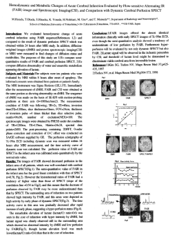


© Copyright 2026