
Interference and diffraction Chapter 9
Chapter 9 Interference and diffraction Copyright 2010 by David Morin, [email protected] (Version 1, June 25, 2010) This file contains the “Interference and diffraction” chapter of a potential book on Waves, designed for college sophomores. In this chapter we’ll study what happens when waves from two or more sources exist at a given point in space. In the case of two waves, the total wave at the given point is the sum of the two waves. The waves can add constructively if they are in phase, or destructively if they are out of phase, or something inbetween for other phases. In the general case of many waves, we need to add them all up, which involves keeping track of what all the phases are. The results in this chapter basically boil down to (as we’ll see) getting a handle on the phases and adding them up properly. We won’t need to worry about various other wave topics, such as dispersion, polarization, and so on; it pretty much all comes down to phases. The results in this chapter apply to any kind of wave, but for convenience we’ll generally work in terms of electromagnetic waves. The outline of this chapter is as follows. In Section 9.1 we do the warm-up case of two waves interfering. The setup consists of a plane wave passing through two very narrow (much narrower than the wavelength of the wave) slits in a wall, and these two slits may be considered to be the two sources. We will calculate the interference pattern on a screen that is located far away. We’ll be concerned with this “far-field” limit for most of this chapter, with the exception of Section 9.5. In Section 9.2 we solve the general case of interference from N narrow slits. In addition to showing how the phases can be added algebraically, we show how they can be added in an extremely informative geometric manner. In Section 9.3 we switch gears from the case of many narrow slits to the case of one wide slit. The word “diffraction” is used to describe the interference pattern that results from a slit with nonnegligible width. We will see, however, that this still technically falls into the category of N narrow slits, because one wide slit can be considered to be a collection of a large (infinite) number of narrow slits. In section 9.4 we combine the results of the two previous sections and calculate the interference pattern from N wide slits. Finally, in Section 9.5 we drop the assumption that the screen is far away from the slit(s) and discuss “near-field” interference and diffraction. This case is a bit more complicated, but fortunately there is still a nice geometric way of seeing how things behave. This involves a very interesting mathematical curve known as the Cornu spriral. 1 2 plane wave 9.1 CHAPTER 9. INTERFERENCE AND DIFFRACTION Two-slit interference Consider a plane wave moving toward a wall, and assume that the wavefronts are parallel to the wall, as shown in Fig. 1. If you want, you can consider this plane wave to be generated by a point source that is located a very large distance to the left of the wall. Let there be two very small slits in the wall that let the wave through. (We’ll see in Section 9.3 that by “very small,” we mean that the height is much smaller than the wavelength.) We’re assuming that the slits are essentially infinite in length in the direction perpendicular to the page. So they are very wide but very squat rectangles. Fig. 2 shows a head-on view from the far-away point source. wall Figure 1 (view from distant source) wall slits wall wall infinitely wall extends in both directions wall extends infinitely in both directions Figure 2 A B By Huygens’ principle we can consider each slit to be the source of a cylindrically propagating wave. It is a cylindrical (and not spherical) wave because the wave has no dependence in the direction perpendicular to the page, due to the fact that it is generated by a line source (the slit). If we had a point source instead of a line source, then we would end up with a standard spherically propagating wave. The reason why we’re using a line source is so that we can ignore the coordinate perpendicular to the page. However, having said this, the fact that we have a cylindrical wave instead of a spherical wave will be largely irrelevant in this √ chapter. The main difference is that the amplitude of a cylindrical wave falls off like 1/ r (see Section [to be added] in Chapter 7) instead of the usual 1/r for a spherical wave. But for reasons that we will see, we can usually ignore this dependence. In the end, since we’re ignoring the coordinate perpendicular to the page, we can consider the setup to be a planer one (in the plane of the page) and effectively think of the line source as a point source (namely, the point on the√line that lies in the page) that happens to produce a wave whose amplitude falls off like 1/ r (although this fact won’t be very important). The important thing to note about our setup is that the two sources are in phase due to the assumption that the wavefronts are parallel to the wall.1 Note that instead of this setup with the incoming plane wave and the slits in a wall, we could of course simply have two actual sources that are in phase. But it is sometimes difficult to generate two waves that are exactly in phase. Our setup with the slits makes this automatically be the case. As the two waves propagate outward from the slits, they will interfere. There will be constructive interference at places where the two waves are in phase (where the pathlengths from the two slits differ by an integral multiple of the wavelength). And there will be destructive interference at places where the two waves are 180◦ out of phase (where the pathlengths from the two slits differ by an odd multiple of half of the wavelength). For example, there is constructive interference at point A in Fig. 3 and destructive interference at point B. What is the interference pattern on a screen that is located very far to the right of the wall? Assume that the screen is parallel to the wall. The setup is shown in Fig. 4. The distance between the slits is d, the distance to the screen is D, the lengths of the two paths to a given point P are r1 and r2 , and θ is the angle that the line to P makes with the normal to the wall and screen. The distance x from P to the midpoint of the screen is then x = D tan θ. Figure 3 1 Problem 9.1 shows how things are modified if the wavefronts aren’t parallel to the wall. This is done in the context of the N -slit setup in Section 9.2. The modification turns out to be a trivial one. 9.1. TWO-SLIT INTERFERENCE 3 wall essentially parallel screen P r1 S1 x θ d r2 S2 D Figure 4 In finding the interference pattern on the screen, we will work in the so-called far-field limit where the screen is very far away. (We’ll discuss the near-field case in Section 9.5.)2 The quantitative definition of the far-field limit is D À d. This assumption that D is much larger than d leads to two important facts. • If D À d, then we can say that the two pathlengths r1 and r2 in Fig. 4 are essentially equal in a multiplicative sense. That is, the ratio r1 /r2 is essentially equal to 1. This follows from the fact that the additive difference |r1 − r2 | is negligible compared with r1 and r2 (because |r1 − r2 | can’t be any larger than d, which we are assuming is negligible compared with D, which itself is less than r1 and r2 ). This r1 /r2 ≈ 1 fact then tells us that the amplitudes of the two waves at point P √from the two slits are essentially equal (because the amplitudes are proportional to 1/ r, although the exact power dependence here isn’t important). • If D À d, then we can say that the r1 and r2 paths in Fig. 4 are essentially parallel, and so they make essentially the same angle (namely θ) with the normal. The parallel nature of the paths then allows us to easily calculate the additive difference between the pathlengths. A closeup of Fig. 4 near the slits is shown in Fig. 5. The difference in the pathlengths is obtained by dropping the perpendicular line as shown, so we see that the difference r2 − r1 equals d sin θ. The phase difference between the two waves is then 2π d sin θ k(r2 − r1 ) = kd sin θ = d sin θ = 2π · . (1) λ λ In short, d sin θ/λ is the fraction of a cycle that the longer path is ahead of the shorter path. Remark: We found above that r1 is essentially equal to r2 in a multiplicative sense, but not in an additive sense. Let’s be a little more explicit about this. Let ² be defined as the difference, ² ≡ r2 − r1 . Then r2 = r1 + ², and so r2 /r1 = 1 + ²/r1 . Since r1 > D, the second term here is less than ²/D. As we mentioned above, this quantity is negligible because ² can’t be larger than d, and because we’re assuming D À d. We therefore conclude that r2 /r1 ≈ 1. In other words, r1 ≈ r2 in a multiplicative sense. This then implies that the amplitudes of the two waves are essentially equal. However, the phase difference equals k(r2 − r1 ) = 2π(r2 − r1 )/λ = 2π²/λ. So if ² is of the same order as the wavelength, then the phase difference isn’t negligible. So r2 is not equal to r1 2 The fancier terminology for these two cases comes from the people who did pioneering work in them: the Fraunhofer limit for far-field, and the Fresnel limit for near-field. The correct pronunciation of “Fresnel” appears to be fray-NELL, although many people say freh-NELL. n cree to s away far S1 d S2 θ θ d sinθ Figure 5 4 CHAPTER 9. INTERFERENCE AND DIFFRACTION in an additive sense. To sum up, the multiplicative comparison of r2 and r1 (which is relevant for the amplitudes) involves the comparison of ² and D, and we know that ²/D is negligible in the far-field limit. But the additive comparison of r2 and r1 (which is relevant for the phases) involves the comparison of ² and λ, and ² may very well be of the same order as λ. ♣ Having found the phase difference in Eq. (1), we can now find the total value of the wave at point P . Let AP be the common amplitude of each of the two waves at P . Then up to an overall phase that depends on when we pick the t = 0 time, the total (complex) wave at P equals Etot (P ) = = AP ei(kr1 −ωt) + AP ei(kr2 −ωt) AP (eikr1 + eikr2 )e−iωt . (2) Our goal is to find the amplitude of the total wave, because that (or rather the square of it) yields the intensity of the total wave at point P . We can find the amplitude by factoring out the average of the two phases in the wave, as follows. ³ ´ Etot (P ) = AP eik(r1 −r2 )/2 + e−ik(r1 −r2 )/2 eik(r1 +r2 )/2 e−iωt µ ¶ ¡ ¢ k(r1 − r2 ) i k(r1 +r2 )/2−ωt = 2AP cos e 2 ¶ ¡ µ ¢ kd sin θ ei k(r1 +r2 )/2−ωt , (3) = 2AP cos 2 where we have used k(r2 − r1 ) = kd sin θ from Eq. (1). The amplitude is the coefficient of the exponential term, so we see that the total amplitude at P is µ ¶ µ ¶ kd sin θ kd sin θ Atot (P ) = 2AP cos −→ Atot (θ) = 2A(θ) cos , (4) 2 2 where we have rewritten AP as A(θ), and Atot (P ) as Atot (θ), to emphasize the dependence on θ. Note that the amplitude at θ = 0 is 2A(0) cos(0) = 2A(0). Therefore, Atot (θ) A(θ) = cos Atot (0) A(0) µ kd sin θ 2 ¶ (5) The intensity is proportional to the square of the amplitude, which gives Itot (θ) A(θ)2 = cos2 Itot (0) A(0)2 µ kd sin θ 2 ¶ (6) √ Since the amplitude of a cylindrically propagating wave is proportional to 1/ r, we have s s p √ 1/ r(θ) A(θ) r(0) D = p = = = cos θ. (7) A(0) r(θ) D/ cos θ 1/ r(0) Therefore, Itot (θ) Itot (0) µ ¶ kd sin θ 2 µ ¶ πd sin θ = cos θ cos2 . λ = cos θ cos2 (8) 9.1. TWO-SLIT INTERFERENCE 5 This result holds for all values of θ, even ones that approach 90◦ . The only approximation we’ve made so far is the far-field one, which allows us to say that (1) the amplitudes of the waves from the two slits are essentially equal, and (2) the two paths are essentially parallel. The far-field approximation has nothing to do with the angle θ. If we want to write Itot in terms of√the distance x from the√midpoint of the screen, instead of θ, then we can use cos θ = D/ x2 + D2 and sin θ = x/ x2 + D2 . This gives µ ¶ Itot (x) D xkd 2 √ √ = cos Itot (0) x2 + D2 2 x2 + D2 µ ¶ D xπd 2 √ √ = cos . (9) x2 + D2 λ x2 + D2 Plots of Itot (x)/Itot (0) are shown in Fig. 6, for d values of (.01)λ, (0.5)λ, 5λ, and 50λ. I(x)/I(0) I(x)/I(0) 1.0 1.0 (d = .01 λ) 0.8 (d = 0.5 λ) 0.8 0.6 0.6 0.4 0.4 0.2 0.2 x/D -4 -2 0 2 x/D -4 4 -2 I(x)/I(0) 2 4 I(x)/I(0) 1.0 1.0 (d = 5λ) 0.8 0 (d = 50λ) 0.8 0.6 0.6 0.4 0.4 0.2 0.2 x/D -4 -2 0 2 4 x/D -4 -2 0 2 4 Figure 6 As you can see from the first plot, if d is much smaller than λ, the interference pattern isn’t too exciting, because the two paths are essentially in phase with each other. The most they can be out of phase is when θ → 90◦ (equivalently, x → ∞), in which case the pathlength difference is simply b = (.01)λ, which is only 1% of a full phase. Since we have d ¿ λ in the first plot, the cosine-squared term √ in Eq. (9) is essentially equal to 1, so the curve reduces to a plot of the function D/ x2 + D2 . It decays to zero for the simple intuitive reason that the farther √ we get away from the slit, the smaller the amplitude is (more precisely, A(θ) = A(0) cos θ). In this d ¿ λ case, we effectively have a single light source from a single slit; interference from the two slits is irrelevant because the waves can never be much out of phase. The function in the first plot is simply the intensity we would see from a single slit. The d = (0.5)λ plot gives the cutoff case when there is barely destructive interference at x = ∞. (Of course, the amplitude of both waves is zero there, so the total intensity is zero anyway.) The d = 5λ and d = 50λ plots exhibit noticeable interference. The local maxima occur where the two pathlengths differ by an integral multiple of the wavelength. The local minima √ occur where the two pathlengths differ by an odd multiple of half of the wavelength. function in Eq. (9) is the envelope of the cosine-squared function. In the The D/ x2 + D2 √ first plot, the D/ x2 + D2 function is all there is, because the cosine-squared function I(x)/I(0) 6 1.0 0.8 0.6 0.4 0.2 x/D - 0.2 - 0.1 0.0 0.1 0.2 (d = 50λ) Figure 7 CHAPTER 9. INTERFERENCE AND DIFFRACTION essentially never deviates from 1. But in the d = 5λ and d = 50λ cases, it actually goes through some cycles. Fig. 7 shows a close-up √ version of the d = 50λ case. For small x (equivalently, for small θ), the ratio A(θ)/A(0) = cos θ is essentially equal to 1, so the envelope is essentially constant. We therefore simply have a cosine-squared function with a nearly-constant amplitude. In practice, we’re usually concerned only with small x and θ values, in which case Eqs. (8) and (9) become Itot (θ) ≈ cos2 Itot (0) Itot (x) ≈ cos2 Itot (0) I(x)/I(0) µ µ θπd λ xπd λD ¶ (for θ ¿ 1) (for x ¿ D) ¶ (10) 1.0 0.8 0.6 0.4 0.2 x 0 2λD λD ____ ___ d d Figure 8 For the remainder of this chapter, we will generally work in this small-angle approximation. So we won’t need the exact (at least exact in the far-field approximation) results in Eqs. (8) and (9). The plot of Itot (x)/Itot (0) from Eq. (10) is shown in Fig. 8. The maxima occur at integer multiples of λD/d. It makes sense that the spacing grows with λ, because the larger λ is, the more tilted the paths in Fig. 5 have to be to make the difference in their lengths (which is d sin θ) be a given multiple of λ. The approximations we’ve made in Fig. 8 are that we’ve ignored the facts that as we move away from the center of the screen, (a) the amplitude A(θ) of the two waves decreases, and (b) the peaks become spaced farther apart. You can compare Fig. 8 with the third and fourth plots in Fig. 6. Remember that the small-angle approximation we’ve made here is different from the “far-field” approximation. The far-field approximation is the statement that the distances from the two slits to a given point P on the screen are essentially equal, multiplicatively. This holds if d ¿ D. (We’ll eventually drop this assumption in Section 9.5 when we discuss the near-field approximation.) The small-angle approximation that leads to Eq. (10) is the statement that the distances from the two slits to different points on the screen are all essentially equal. This holds if x ¿ D, or equivalently θ ¿ 1. Note that the small-angle approximation has no chance of being valid unless the far-field approximation already holds. Remark: The small-angle approximation in Eq. (10) shoves the A(θ) dependence in Eq. (6) under the rug. Another way to get rid of this dependance is to use a cylindrical screen instead of a flat screen, with the axis of the cylinder coinciding with the slits. So in Fig. 4 the screen would be represented by a semicircle in the plane of the page, with the slits located at the center. In the far-field limit, all of the paths in different θ directions now have the same length, multiplicatively. (The difference in pathlengths to a given point on the screen is still d sin θ.) So A(θ) = A(0) for all θ, and the A’s cancel in Eq. (6). Note, however, that the spacing between the local maxima on the cylindrical screen still isn’t uniform, because they occur where sin θ = λ/d. And sin θ isn’t a linear function of θ. At any rate, the reason why we generally work in terms of a flat screen isn’t that there is anything fundamentally better about it compared with a cylindrical screen. It’s just that in practice it’s easier to find a flat screen. ♣ 9.2 N -slit interference 9.2.1 Standard derivation Let’s now looks at the case where we have a general number, N , of equally-spaced slits, instead of 2. The setup is shown in Fig. 9 for the case of N = 5. 9.2. N -SLIT INTERFERENCE 7 wall screen P r1 d d d d rN Figure 9 Similar to the N = 2 case above, we will make the far-field assumption that the distance to the screen is much larger than the total span of the slits, which is (N − 1)d. We can then say, as we did in the N = 2 case, that all the paths to a given point P on the screen have essentially the same length in a multiplicative (but not additive) sense, which implies that the amplitudes of the waves are all essentially equal. And we can also say that all the paths are essentially parallel. A closeup version near the slits is shown in Fig. 10. Additively, each pathlength is d sin θ longer than the one right above it. So the lengths take the form of rn = r1 + (n − 1)d sin θ. To find the total wave at a given point at an angle θ on the screen, we need to add up the N individual waves (call them En ). The procedure is the same as in the N = 2 case, except that now we simply have more terms in the sum. In the N = 2 case we factored out the average of the phases (see Eq. (3)), but it will now be more convenient to factor out the phase of the top wave in Fig. 9 (the r1 path). The total wave at an angle θ on the screen is then (with A(θ) being the common amplitude of all the waves) Etot (θ) = N X En = n=1 N X A(θ)e i(kr1 −ωt) A(θ)e N X = = d Figure 10 e ik(n−1)d sin θ . (11) With z ≡ eikd sin θ , the sum here is 1 + z + z 2 + · · · + z N −1 . The sum of this geometric series is = d sinθ d θ n=1 zN − 1 z−1 d θ d i(krn −ωt) n=1 = n cree to s away far eikN d sin θ − 1 eikd sin θ − 1 eik(N/2)d sin θ eik(N/2)d sin θ − e−ik(N/2)d sin θ · eik(1/2)d sin θ eik(1/2)d sin θ − e−ik(1/2)d sin θ ¡1 ¢ ik((N −1)/2)d sin θ sin ¡2 N kd sin θ ¢ . e · sin 12 kd sin θ Substituting this into Eq. (11) yields a total wave of ¢ ¡ sin 12 N kd sin θ ³ i(kr1 −ωt) ik((N −1)/2)d sin θ ´ ¡ ¢ e . e Etot (θ) = A(θ) sin 12 kd sin θ The amplitude is the coefficient of the exponential factors, so we have ¡ ¢ sin 12 N kd sin θ sin(N α/2) ¡1 ¢ ≡ A(θ) Atot (θ) = A(θ) sin(α/2) sin 2 kd sin θ (12) (13) (14) 8 CHAPTER 9. INTERFERENCE AND DIFFRACTION where 2πd sin θ . (15) λ Since adjacent pathlengths differ by d sin θ, the physical interpretation of α is that it is the phase difference between adjacent paths. What is the value of Atot (θ) at the midpoint of the screen where θ = 0 (which implies α = 0)? At α = 0, Eq. (14) yields Atot (θ) = 0/0, which doesn’t tell us much. But we can obtain the actual value by taking the limit of small α. Using sin ² ≈ ², we have α ≡ kd sin θ = Atot (0) = lim Atot (θ) = lim A(θ) α→0 θ→0 sin(N α/2) N α/2 = A(0) = A(0) · N. sin(α/2) α/2 (16) It is customary to deal not with the amplitude itself, but rather with the amplitude relative to the amplitude at θ = 0. Combining Eqs. (14) and (16) gives Atot (θ) A(θ) sin(N α/2) = · . Atot (0) A(0) N sin(α/2) (17) Since we generally deal with small angles, we’ll ignore the variation in the A(θ) coefficient. In other words, we’ll set A(θ) ≈ A(0). This gives Atot (α) sin(N α/2) ≈ Atot (0) N sin(α/2) (for small θ) (18) The intensity at θ relative to the intensity at θ = 0 is then Itot (α) ≈ Itot (0) µ sin(N α/2) N sin(α/2) ¶2 (for small θ) (19) Even for large angles, the effect of A(θ) is to simply act as an envelope function of the oscillating sine functions. We can always bring A(θ) back in if we want to, but the more interesting behavior of Atot (θ) is the oscillatory part. We’re generally concerned with the locations of the maxima and minima of the oscillations and not with the actual value of the amplitude. The A(θ) factor doesn’t affect these locations.3 We’ll draw a plot of what Itot (α)/Itot (0) looks like, but first a remark. Remark: Technically, we’re being inconsistent here in our small-angle approximation, because although we set A(θ) = A(0) (which from Eq. (7) is equivalent to setting cos θ = 1), we didn’t set sin θ = θ in the expression for α. To be consistent, we should approximate α = kd sin θ by α = kd·θ. The reason why we haven’t made this approximation is that we want to keep the locations of the bumps in the interference pattern correct, even for large θ. And √ besides, the function A(θ) depends on the nature of the screen. A flat screen has A(θ)/A(0) = cos θ, which decreases with θ, while a cylindrical screen has A(θ)/A(0) = 1, which is constant. Other shapes yield other functions of θ. But they’re all generally slowly-varying functions of θ, compared with the oscillations of the sin(N α/2) function (unless you use a crazily-shaped wiggly screen, which you have no good reason to do). The main point is that the function A(θ) isn’t an inherent property of the interference pattern; it’s a property of the screen. On the other hand, the angular locations of the maxima and minima of the oscillations are an inherent property of the pattern. So it makes sense to keep these locations exact and not lose this information when making the small-angle approximation. If you want, you can write the intensity in Eq. (19) as Itot (θ) = F (θ) Itot (0) µ sin(N α/2) N sin(α/2) ¶2 (where α ≡ kd sin θ), (20) 3 Strictly speaking, A(θ) does affect the locations of the maxima in a very slight manner (because when taking the overall derivative, the derivative of A(θ) comes into play). But A(θ) doesn’t affect the locations of the minima, because those are where Itot (α) is zero. 9.2. N -SLIT INTERFERENCE 9 I(α)/I(0) 1.0 0.8 0.6 0.4 0.2 where F (θ) is a slowly-varying function of θ that depends on the shape of the screen. We will generally ignore this dependence and set F (θ) = 1. ♣ What does the Itot (α)/Itot (0) ratio in Eq. (19) look like as a function of α? The plot for N = 4 is shown in Fig. 11. If we’re actually talking about small angles, then we have α = kd sin θ ≈ kd · θ. But the distance from the center of the screen is x = D tan θ ≈ D · θ. So for small angles, we have α ∝ x. You can therefore think of Fig. 11 as showing the actual intensity on the screen as a function of x (up to a scaling constant). Note that although we generally assume θ to be small, α is not necessarily small, because α ≡ kd sin θ involves a factor of k which may be large. Said in another way, α is the phase difference between adjacent slits, so if k is large (more precisely, if λ ¿ d), then even a small angle θ can lead to a pathlength difference (which is d sin θ) equal to λ. This corresponds to a phase difference of α = kd sin θ = (2π/λ)d sin θ = 2π. Consistent with this, the values on the horizontal axis in Fig. 11 are on the order of π (that is, they are not small), and the first side peak is located at 2π. A number of things are evident from both Fig. 11 and Eq. (19): 1. The value of Itot (α)/Itot (0) at θ = 0 is 1, by construction. 2. Itot (α)/Itot (0) has a period of 2π in α. The sine function in the denominator picks up a minus sign when α increases by 2π, and likewise in the numerator if N is odd. But an overall minus sign is irrelevant because the intensity involves the squares of the sines. 3. Itot (α) has zeroes whenever N α/2 is a multiple of π, that is, whenever N α/2 = mπ =⇒ α = 2mπ/N , which means that α is an even multiple of π/N . The one exception to this is when α/2 is also a multiple of π, that is, when α/2 = m0 π =⇒ α = 2m0 π, because then the denominator in Eq. (19) is also zero. (In this case, Eq. (16) tells us that the value at θ = 0 is 1. And likewise at any integer multiple of 2π. These are the locations of the main peaks.) In the N = 4 case in Fig. 11, you can see that the zeros do indeed occur at 0π ¶, 2π , 4π , 6π , 8π ¶, 10π , 12π , 14π , 16π ¡, · · · . ¶ ¶ ¡ 4 4 4 4 4 4 4 4 ¶ ¶ ¡4 (21) And likewise for negative values. In general, the number of zeros between the main peaks is N − 1. 4. If you take the derivative of Itot (α), you will find that the local maxima (of the small bumps) occur when tan(N α/2) = N tan(α/2). This has to be solved numerically. However, for large N , the solutions for α are generally very close to the odd multiples of π/N (except for values of the form of 2π ± π/N ); see Problem [to be added]. In other words, the local maxima are approximately right between the local minima (the zeros) which themselves occur exactly at the even multiples of π/N , except at the integral multiples of 2π where the main peaks are. In Fig. 11 you can see that the small bumps do indeed occur at approximately 1π ¶, 3π , 5π , 7π ¶, 9π ¶, 11π , 13π , 15π ¡, 17π ¡, 19π , · · · . ¶ ¶ ¶ ¡ ¡ 4 4 4 4 4 ¶4 ¶4 ¶4 ¡4 ¡4 (22) And likewise for negative values. In general, the number of little bumps between the main peaks is N − 2. 5. The little bumps in Fig. 11 have the same height, simply because there are only two of them. For larger values of N , the bump sizes are symmetric around α = π (or in α (N = 4) _ π 3π __ 2π π 2 2 Figure 11 I(α)/I(0) 10 1.0 0.8 0.6 0.4 0.2 α (N = 8) general any multiple of π). They are the shortest there (because the denominator in Eq. (19) is largest at α = π), and they grow in size as they get closer to the main peaks. Fig. 12 shows the interference pattern for N = 8. Note that if d < λ, then α ≡ kd sin θ = (2π/λ)d sin θ < 2π sin θ ≤ 2π. So α can’t achieve the value of 2π, which means that none of the tall side peaks in Fig. 11 exist. We have only one tall peak at α = 0, and then a number of small peaks. This makes sense physically, because the main peaks occur when the waves from all the slits are in phase. And if d < λ there is no way for the pathlengths to differ by λ, because the difference can be at most d (which occurs at θ = 90◦ ). In general, the upper limit on α is kd, because sin θ can’t exceed 1. So no matter what the relation between d and λ is, a plot such as the one in Fig. 12 exists out to the α = kd point (which corresponds to θ = 90◦ ), and then it stops. In the case of N = 2, we should check that the expression for Itot (α)/Itot (0) in Eq. (19) reduces properly to the expression in Eq. (6) (with A(θ) set equal to A(0)). Indeed, if N = 2, then the quotient in Eq. (19) becomes sin(2·α/2)/2¡ sin(α/2). Using ¢ the double-angle formula in the numerator turns this into cos(α/2) = cos (1/2)kd sin θ , which agrees with Eq. (6). 2π π CHAPTER 9. INTERFERENCE AND DIFFRACTION Figure 12 9.2.2 Geometric construction Let’s now derive the amplitude in Eq. (14) in a different way. It turns out that there is an extremely informative geometric way of seeing how this amplitude arises. The main task in finding the amplitude is calculating the sum in Eq. (11). With α ≡ kd sin θ, this sum is N X (N=4) ei α α α α 1 Figure 13 Rei φ r 1 α α αα 1 1 1 Figure 14 (23) n=1 ei 2α ei 3α eik(n−1)d sin θ = 1 + eiα + ei2α + · · · + ei(N −1)α . Each term in this sum is a complex number with magnitude 1. If we plot these numbers as vectors in the complex plane, they make angles of 0, α, 2α, etc. with respect to the x axis. For example, in the case of N = 4 we might have the unit vectors shown in Fig. 13. (Remember that α depends on θ, which depends on where the point P is on the screen. So for any point P , we have a set of N vectors in the plane. The angle α between them increases as P moves farther off to the side.) The easiest way to add up these vectors is to put them tail-to-head, as shown in Fig. 14. Each of the unit vectors is tilted at an angle α with respect to the one before it. The desired sum is the thick vector shown. As with any complex number, we can write this sum as a magnitude times a phase, that is, as Reiφ . The total amplitude Atot (θ) equals R times the A(θ) in Eq. (11), because the phase ei(kr1 −ωt) in Eq. (11) and the phase eiφ in the sum don’t affect the amplitude. So our goal is to find R, which can be done in the following way. (If you want to find the value of φ, see Problem [to be added].) The thick vector in Fig. 14 is the base of an isosceles triangle with vertex angle 4α, which in general is N α. So we have R = 2 · r sin(N α/2), (24) where r is the length shown in the figure. But from looking at any one of the four thinner isosceles triangles with vertex angle α and base 1, we have 1 = 2 · r sin(α/2). (25) Taking the quotient of the two preceding equations eliminates the length r, and we arrive at sin(N α/2) . (26) R= sin(α/2) 9.2. N -SLIT INTERFERENCE 11 This reproduces Eq. (14), because the total amplitude Atot (θ) equals R · A(θ). As time increases, the whole picture in Fig. 14 rotates clockwise in the plane, due to the −ωt in the phase. There is also a phase shift due to the k1 r and φ terms in the phase, but this simply affects the starting angle. Since all the little vectors keep their same relative orientation, the figure keeps its same shape. That is, it rotates as a rigid “object.” The sum (the thick vector) therefore always has the same length. This (constant) length is therefore the amplitude, while the (changing) horizontal component is the real part that as usual gives the actual physical wave. The above geometric construction makes it easy to see why the main peaks and all the various local maxima and minima appear in Fig. 12. The main peaks occur when α is a multiple of 2π, because then all the little vectors point in the same direction (rightward at a given instant, if the first little vector points to the right at that instant). The physical reason for this is that α = m · 2π implies that kd sin θ = 2mπ =⇒ 2πd sin θ = 2mπ =⇒ d sin θ = mλ. λ (27) This says that the difference in pathlengths from adjacent slits is a multiple of the wavelength, which in turn says that the waves from all of the slits constructively interfere. Hence the maximal amplitude. A local minimum (a zero) occurs if the value of α is such that the chain of little vectors in Fig. 14 forms a closed regular polygon (possibly wrapped around multiple times). In this case the sum (the thick vector in Fig. 14) has no length, so the amplitude is zero. The “polygons” for the seven zeros in the N = 8 case in Fig. 12 are shown in Fig. 15. We’ve taken the first of the vectors to always point horizontally to the right, although this isn’t necessary. We’ve drawn the figures slightly off from the case where the sum of the vectors is zero, to make it easier to see what’s going on. The last three figures are mirror images of the first three. (α= π/4) (α= π/2) (α= 3π/4) (α= π) (α= 5π/4) Figure 15 (α= 3π/2) (α= 7π/4) 12 CHAPTER 9. INTERFERENCE AND DIFFRACTION The local maxima occur between the local minima. In the case of large N , it’s easy to determine the approximate locations of these maxima. For large N , the vectors form an essentially smooth curve, and the maxima occur roughly when the amplitude is a diameter of a circle. The first few of these occurrences are shown in Fig. 16 for the case of N = 50. We’ve made the curve spiral slightly inward so that you can see how many times it wraps around. But in reality (in the far-field limit), the curve just keeps tracing over itself. (N=50) (α=3π/50) (α=5π/50) (α=7π/50) (α=0 for comparison) Figure 16 The maxima don’t occur exactly at the diameters, because the circle shrinks as the little vectors wrap around further as α increases, so there are competing effects. But it is essentially the diameter if the wrapping number is large (because in this case the circle hardly changes size as the amplitude line swings past the diameter, so the shrinking effect is basically nonexistent). So we want the vectors to wrap (roughly) 3/2, 5/2, 7/2, etc. times around the circle. Since each full circle is worth 2π radians, this implies that the total angle, which is N α, equals 3π, 5π, 7π, etc. In other words, α is an odd multiple of π/N , excluding π/N itself (and also excluding the other multiples adjacent to multiples of 2π). This agrees with the result in the paragraph preceding Eq. (22). The amplitude of the main peaks that occur when α equals zero or a multiple of 2π is also shown in Fig. 16 for comparison. In this case the circular curve is unwrapped and forms a straight line. The little tick marks indicate the N = 50 little vectors. 9.2.3 Diffraction gratings A diffraction grating is a series of a large number, N , of slits with a very small spacing d between them. If a source emits light that consists of various different wavelengths, a diffraction grating provides an extremely simple method for determining what these wavelengths are. As we saw above, the N -slit interference pattern consists of the main peaks, plus many smaller peaks in between. However, we will be concerned here only with the main peaks, because these completely dominate the smaller peaks, assuming N is large. Let’s justify this statement rigorously and discuss a few other things, and then we’ll do an example. From the discussion that led to Eq. (22), the smaller peaks occur when α takes on values that are approximately the odd multiples of π/N (except for values of the form 2π ± π/N ), that is, when α equals 3π/N , 5π/N , etc. The corresponding values of Itot (α)/Itot (0) are obtained from Eq. (19). The numerator equals (±1)2 , and since N is large we can use a 9.2. N -SLIT INTERFERENCE 13 small-angle approximation in the denominator, which turns the denominator into N α/2. The resulting values of Itot (α)/Itot (0) are then (2/3π)2 , (2/5π)2 , etc. Note that these are independent of N . The first of the side peaks isn’t negligible compared with the main peak (it’s about (2/3π)2 = 4.5% as tall). But by the 10th peak, the height is negligible (it’s about 0.1% as tall). However, even though the first few side peaks aren’t negligible, they are squashed very close to the main peaks if N is large. This follows from the fact that the spacing between the main peaks is ∆α = 2π, whereas the side peaks are on the order of π/N away from the main peaks. The figure for N = 20 is shown in Fig. 17. We can therefore make the approximation that the interference pattern is non-negligible only at (or extremely close to) the main peaks where α is a multiple of 2π. When dealing with diffraction gratings, we’re generally concerned only with the location of the bright spots in the interference pattern, and not with the actual intensity. So any extra intensity from the little side peaks is largely irrelevant. And since they’re squashed so close to the main peaks, it’s impossible to tell that they’re distinct bumps anyway. The location of the main peaks tells us what the various wavelengths are, by using kd sin θ = 2π =⇒ (2π/λ)d sin θ = 2π =⇒ λ = d sin θ. The intensity tells us how much of each wavelength the light is made of, but for most purposes we’re not so concerned about this. I(α)/I(0) 1.0 0.8 0.6 0.4 0.2 α -2π 0 2π (N = 20) Figure 17 Remarks: 1. A diffraction grating should more appropriately be called an “interference grating,” because it is simply an example of N -slit interference. It is not an example of diffraction, which we will define and discuss in Section 9.3.1. We’ll see there that a feature of a diffraction pattern is that there are no tall side peaks, whereas these tall side peaks are the whole point of an “interference grating.” However, we’ll still use the term “diffraction grating” here, since this is the generally accepted terminology. 2. If we view the interference pattern on a screen, we know that it will look basically like Fig. 17 (we’ll assume for now that only one wavelength is involved). However, if you put your eye right behind the grating, very close to it, what do you see? If you look straight at the light source, then you of course see the source. But if you look off at an angle (but still through the grating; so your eye has to be close to it), then you will also see a bright spot there. And you will also see bright spots at other angles. The number of spots depends on the relation between the wavelength and the spacing. We’ll discuss a concrete case in the example below. The angles at which you see the spots are the same as the angles of the main peaks in Fig. 17, for the following reason. Fig. 18 shows the typical locations of the first few main peaks in the interference pattern from a standard set of slits contained in a small span in a wall. Imagine putting additional sets of slits in the wall at locations such that a given spot on the screen (your eye) is located at the angles of successive off-center peaks. This scenario is shown in Fig. 19. Each set of slits also produces many other peaks, of course, but you don’t see them because your eye is at only one location. A diffraction grating is a continuous set of slits, but most of the slits are irrelevant. The only slits that matter are the ones that are located at positions such that the angle to your eye is one of the main-peak angles. In other words, we can replace the entire wall in Fig. 19 with a continuous set of slits, and you will still see the same thing. Only the small regions of slits shown in the figure will produce bright spots. In short, a diffraction grating acts like a collection of interference setups at specific locations in the grating. 3. You might be concerned that if your eye is close enough to the grating, then the far-field approximation (and hence all of the result so far in this chapter) will be invalid. After all, the distance D from your eye to the grating isn’t large compared with the total span of the slits in the grating. However, the far-field approximation does indeed still hold, because from the previous remark we’re not concerned with the total span of the slits in the grating, but rather with the span of a small region near each of the main-peak angles. Assuming that the spacing between the lines in the grating is very small (it’s generally on the order of 10−6 m), the span directions of first few maxima θ1 θ2 Figure 18 θ2 θ1 eye Figure 19 14 CHAPTER 9. INTERFERENCE AND DIFFRACTION of a few hundred lines will still be very small compared with the distance from your eye to the grating (assuming that your eyelashes don’t touch it). So the far-field approximation still holds. That is, the distances from these few hundred slits to your eye are all essentially equal (multiplicatively). 4. In reality, most diffraction gratings are made by etching regularly-spaced lines into the material. The exact details of the slits/etchings are’t critical. Any periodic structure with period d will do the trick. The actual intensities depend on the details, but the locations of the main peaks don’t. This follows from the usual argument that if d sin θ is a multiple of λ, then there is constructive interference from the slits (whatever they may look like). 5. Problem 9.1 shows that it doesn’t matter whether or not the incident light is normal to the wall (which is the diffraction grating here), as long as the deviation angle is small. If we measure all angles relative to the incident angle, then all of our previous result still hold. This is fortunate, of course, because if you hold a diffraction grating in front of your eye, it is highly unlikely that you will be able orient it at exactly a 90◦ angle to the line between it and the light source. ♣ Example (Blue and red light): A diffraction grating has 5000 lines per cm. Consider a white-light source (that is, it includes all wavelengths), and assume that it is essentially a point source far away. Taking the wavelengths of blue and red light to be roughly 4.5·10−5 cm and 7 · 10−5 cm, find the angles at which you have to look to the side to see the off-center blue and red maxima. What is the total number of maxima for each color that you can theoretically see on each side of the light source? Solution: We basically have to do the same problem here twice, once for blue light and once for red light. As usual, the main peaks occur where the difference in pathlengths from adjacent slits is an integral multiple of the wavelength. So we want d sin θ = mλ. (Equivalently, we want α = m · 2π, which reduces to d sin θ = mλ.) We therefore want sin θ = mλ/d, where d = (1 cm)/5000 = 2 · 10−4 cm. For blue light, this gives sin θ = m(4.5 · 10−5 cm)/(2 · 10−4 cm) = m(0.225). So we have the following four possible pairs of m and θ values: (m, θ) : (1, 13.0◦ ) (2, 26.7◦ ) (3, 42.5◦ ) (4, 64.2◦ ) (28) There are only four possible angles (plus their negatives), because m = 5 gives a value of sin θ that is larger than 1. For red light, we have sin θ = m(7 · 10−5 cm)/(2 · 10−4 cm) = m(0.35). So we have the following two possible pairs of m and θ values: to far away source grating θ=0 bands 1 1 2 13.0 3 20.5 2 26.7 42.5 44.4 4 64.2 eye θ = 90 Figure 20 (m, θ) : (1, 20.5◦ ) (2, 44.4◦ ) (29) There are only two possible angles (plus their negatives), because m = 3 gives a value of sin θ that is larger than 1. The red angles are larger than the corresponding blue angles because the red wavelength is longer, so it takes a larger angle to make adjacent pathlengths differ by a wavelength (or two wavelengths, etc.). The rest of the spectrum falls between blue and red, so we obtain rainbow bands of colors. Note, however, that the first band (from 13.0◦ to 20.5◦ , although the endpoints are fuzzy) is the only “clean” band that doesn’t overlap with another one. The second band ends at 44.4◦ , which is after the third band starts at 42.5◦ . And the third band doesn’t even finish by the time the angle hits 90◦ . Your viewing angle has to be less than 90◦ , of course, because you have to be looking at least a little bit toward the grating. The angles of the various bands are shown in Fig. 20. The mirror images of these angles on the left side work too. 9.3. DIFFRACTION FROM A WIDE SLIT 9.3 9.3.1 15 Diffraction from a wide slit Derivation We’ll now discuss what happens when a plane wave impinges on just one wide slit with width a, instead of a number of infinitesimally thin ones. See Fig. 21. We’ll find that if the width a isn’t negligible compared with the wavelength λ, then something interesting happens. The interference pattern will depend on a in a particular way, whereas it didn’t depend on the infinitesimal width in the previous sections. We’ll keep working in the far-field limit, which here means that D À a. wall screen P a θ D Figure 21 By Huygen’s principle, we can consider the wide slit to consist of an infinite number of line sources (or point sources, if we ignore the direction perpendicular to the page) next to each other, each creating a cylindrical wave. In other words, the diffraction pattern from one continuous wide slit is equivalent to the N → ∞ limit of the N -slit result in Eq. (19). So we’ve already done most of the work we need to do. We’ll present three ways we can go about taking the continuum limit. But first some terminology. The word diffraction refers to a situation with a continuous aperture. The word interference refers to a situation involving two or more apertures whose waves interfere. On one hand, since diffraction is simply the N → ∞ limit of interference, there is technically no need to introduce a new term for it. But on the other hand, a specific kind of pattern arises, so it makes sense to give it its own name. Of course, we can combine interference and diffraction by constructing a setup with waves coming from a number of wide apertures. We’ll deal with this in Section 9.4. A name that causes confusion between the words “interference” and “diffraction” is the diffraction grating that we discussed above. As we mentioned in the first remark in Section 9.2.3, this should technically be called an interference grating. N → ∞ limit For our first derivation of the diffraction pattern, we’ll take the N → ∞ limit of Eq. (19). The α in Eq. (19) equals kd sin θ. But if we imagine the slit of width a to consist of N infinitesimal slits separated by a distance d = a/N , then we have α = k(a/N ) sin θ. 4 (The N here should perhaps be N − 1, depending on where you put the slits, but this is irrelevant 4 Of course, if we actually have infinitesimal slits separated by little pieces of wall, then the intensity will go down. But this doesn’t matter since our goal is only to find the relative intensity Itot (θ)/Itot (0). As we’ll see below, if the distance d = a/N is much smaller than the wavelength (which it is, in the N → ∞ limit) then we actually don’t even need to have little pieces of wall separating the slits. The slits can bump right up against each other. 16 CHAPTER 9. INTERFERENCE AND DIFFRACTION in the N → ∞ limit.) Plugging this value of α into Eq. (19) gives Itot (θ) ≈ Itot (0) à sin ¡ ka sin θ ¢ !2 N sin ¡ ka2 sin θ ¢ . (30) 2N In the N → ∞ limit, we can use sin ² ≈ ² in the denominator to obtain Itot (θ) ≈ Itot (0) à sin ¡1 2 ka sin θ 1 2 ka sin θ ¢ !2 =⇒ Itot (θ) ≈ Itot (0) µ sin(β/2) β/2 ¶2 (31) where 2πa sin θ . (32) λ Another convention is to define β ≡ (1/2)ka sin θ, in which case the result in Eq. (31) takes ¡ ¢2 the simpler form of (sin β)/β . The reason why we chose β ≡ ka sin θ here is because it parallels the definition of α in Eq. (15). The results in Eqs. (19) and (31) are then similar, in that they both involve factors of 2. The physical meaning of α in Eq. (15) is that it is the phase difference between adjacent paths. The physical meaning of β is that is it the phase difference between the paths associated with the endpoints of the wide slit of width a. The function (sin x)/x is knows as the “sinc” function, sinc(x) ≡ (sin x)/x. A plot is shown in Fig. 22. It is a sine function with a 1/x envelope. The result in Eq. (31) can therefore be written as Itot (θ)/Itot (0) = sinc2 (β/2). A plot of this is shown in Fig. 23. The factor of 2 in the argument makes the plot expanded by a factor of 2 in the horizontal direction compared with the plot in Fig. 22. Since sin θ can’t exceed 1, β can’t exceed ka. So the plot in Fig. 23 exists out to the β = ka point (which corresponds to θ = 90◦ ), and then it stops. Note that the diffraction pattern has only one tall bump, whereas the interference patterns we’ve seen generally have more than one tall bump (assuming that d > λ). This is consistent with the discussion in the second-to-last paragraph in Section 9.2.1. We saw there that if d < λ, then there is only one tall bump. And indeed, in the present case we have d = a/N , which becomes infinitesimal as N → ∞. So d is certainly smaller than λ. The zeros of Itot (θ) occur when β is a multiple of 2π (except β = 0). And since β ≡ 2πa sin θ/λ, this is equivalent to a sin θ being a multiple of λ. We’ll give a physical reason for this relation below in Section 9.3.2, but first let’s give two other derivations of Eq. (31). β ≡ ka sin θ = sinc(x) 1.0 0.8 0.6 0.4 0.2 x 0.2 2π 4π 6π Figure 22 sinc2(β/2) 1.0 0.8 0.6 0.4 0.2 2π 4π 6π 0.2 β Figure 23 Geometric derivation r β rβ 2r sin(β/2) Figure 24 We can give another derivation of the diffraction pattern by using the geometric construction in Section 9.2.2. In the N → ∞ limit, the little vectors in Fig. 14 become infinitesimal, so the crooked curve becomes a smooth curve with no kinks. If β = 0 (which corresponds to θ = 0 and hence α = 0 in Fig. 14), then all of the infinitesimal vectors are in phase, so we get a straight line pointing to the right. If β is nonzero, then the vectors curl around, and we get something like the picture shown in Fig. 24. The bottom infinitesimal vector corresponds to one end of the wide slit, and the top infinitesimal vector corresponds to the other end. The pathlength difference between the ends is a sin θ, so the phase difference is ka sin θ, which is by definition β. This phase difference is the angle between the top and bottom vectors in Fig. 24. But this angle equals the central angle subtended by the arc. The central angle is therefore β, as shown. Now, the amplitude Atot (0) is the length of the straight line in the β = 0 case. But this is also the length of the arc in Fig. 24, which we know is rβ, where r is the radius of the circle. And Atot (θ) is the sum of all the infinitesimal vectors, which is the straight line 9.3. DIFFRACTION FROM A WIDE SLIT 17 shown. From the isosceles triangle in the figure, this sum has length 2r sin(β/2). Therefore, since the intensity is proportional to the square of the amplitude, we have Itot (θ) = Itot (0) µ 2r sin(β/2) rβ ¶2 µ = sin(β/2) β/2 ¶2 , (33) in agreement with Eq. (31). Continuous integral We can also find the diffraction pattern by doing a continuous integral over all the phases from the possible paths from different parts of the wide slit. Let the slit run from y = −a/2 to y = a/2. And let B(θ) dy be the amplitude that would be present at a location θ on the screen if only an infinitesimal slit of width dy was open. So B(θ) is the amplitude (on the screen) per unit length (in the slit). B(θ) dy is the analog of the A(θ) in Eq. (11). If we measure the pathlengths relative to the midpoint of the slit, then the path that starts at position y is shorter by y sin θ (so it is longer if y < 0). It therefore has a relative phase of e−iky sin θ . Integrating over all the paths that emerge from the different values of y (through imaginary slits of width dy) gives the total wave at position θ on the screen as (up to an overall phase from the y = 0 point, and ignoring the ωt part of the phase) Z a/2 Etot (θ) = ¡ ¢ B(θ) dy e−iky sin θ . (34) −a/2 √ This is the continuous version of the discrete sum in Eq. (11). B(θ) falls off like 1/ r, where r = D/ cos θ. However, as in Section 9.2.1, we’ll assume that θ is small, which mean that we can let cos θ ≈ 1. (And even if θ isn’t small, we’re not so concerned about the exact intensities and the overall envelope of the diffraction pattern.) So we’ll set B(θ) equal to the constant value of B(0). We therefore have Z a/2 Etot (θ) ≈ B(0) e−iky sin θ dy −a/2 ´ B(0) ³ −ik(a/2) sin θ e − eik(a/2) sin θ −ik sin θ ¡ ¢ θ −2i sin ka sin 2 = B(0) · −ik sin θ ¡ ¢ sin 12 ka sin θ = B(0)a · . 1 2 ka sin θ = (35) There aren’t any phases here, so this itself is the amplitude Atot (θ). Taking the usual limit at θ = 0, we obtain Atot (0) = B(0)a. Therefore, Atot (θ)/Atot (0) = sin(β/2)/(β/2), where β ≡ ka sin θ. Since the intensity is proportional to the square of the amplitude, we again arrive at Eq. (31). 9.3.2 Width of the diffraction pattern From Fig. 23, we see that most of the intensity of the diffraction pattern is contained within the main bump where |β| < 2π. Numerically, you can shown that the fraction of the total area that lies under the main bump is about 90%. So it makes sense to say that the angular half-width of the pattern is given by β = 2π =⇒ 2πa sin θ = 2π =⇒ λ sin θ = λ a (36) 18 CHAPTER 9. INTERFERENCE AND DIFFRACTION For small θ, this becomes λ (for small θ) (37) a Note that this is inversely proportional to a. The narrower the slit, the wider the diffraction pattern. There are two ways of understanding the sin θ = λ/a result, or equivalently why the intensity is zero when this relation holds. θ≈ β=2π • As indicated in Eq. (36), sin θ = λ/a is equivalent to β = 2π. So in the geometric construction that led to Eq. (33), this means that the arc in Fig. 24 is actually a full circle, as shown in Fig. 25. The sum of all the infinitesimal vectors is therefore zero, so the amplitude and intensity are zero. Figure 25 n cree to s away far θ a θ Imagine dividing the slit into two halves, as shown in Fig. 27. For every path in the upper half (the lightly shaded region), there is a path in the lower half (the darkly shaded region) that is λ/2 longer. So the two waves are exactly out of phase. Three pairs of dotted lines are shown. The waves therefore cancel in pairs throughout the slit, and we end up with zero amplitude. This is equivalent to saying that the phases cancel at diametrically opposite points in Fig. 25. a sinθ = λ Figure 26 a (a/2) sinθ = λ/2 Figure 27 y = β/2 y y = tanβ/2 20 15 10 5 -5 -10 -15 β π 3π 5π Figure 28 7π • If sin θ = λ/a, then the pathlength from one end of the slit is a sin θ = λ longer than the pathlength from the other end, as shown in Fig. 26. So the waves from the two ends are in phase. You might think that this implies that there should be constructive interference (which would be the case if we simply had two infinitesimal slits separated by a). But in fact it’s exactly the opposite in the present case of a continuous wide slit. We have complete destructive interference when the whole slit is taken into account, for the following reason. You can quickly show by taking a derivative that the local maxima of I(β)/I(0) = ¡ ¢2 (sin(β/2))/(β/2) occur when tan β/2 = β/2. This must be solved numerically, but you can get a sense of what the roots are by plotting the functions y = β/2 and y = tan β/2, and then looking at where the curves intersect. In Fig. 28 the intersections are indicated by the dots, and you can see that the associated β values (in addition to the β = 0 root) are close to 3π, 5π, 7π, etc. (the larger β is, the better these approximations are). These maxima therefore occur roughly halfway between the zeros, which themselves occur when β equals (exactly) 2π, 4π, 6π, etc. The task of Problem [to be added] is to show how the 3π, 5π, 7π, etc. values follow from each of the above two bullet-point reasonings. The (half) angular spread of the beam, θ ≈ λ/a, is large if a is small. Physically, the reason for this is that if a is small, then the beam needs to tilt more in order to generate the path differences (and hence phase differences) that lead to the total cancelation at the first zero (at β = 2π). Said in a different way, if a is small, then the beam can tilt quite a bit and still have all the different paths be essentially in phase. If a < λ, then even if the beam is titled at θ = π/2, there still can’t be total cancelation. So if a < λ, then the diffraction pattern has no zeros. It simply consists of one bump that is maximum at θ = 0 and decreases as θ → π/2. It actually does approach zero in this limit (assuming we have a flat screen and not a cylindrical one) because of the B(θ) factor in Eq. (34). θ → π/2 corresponds to points on the screen that are very far from the slit, so the amplitude of all the waves is essentially zero. In the limit a ¿ λ, all of the waves from the different points in the slit are essentially in phase for any angle θ. Interference effects therefore don’t come into play, so the slit behaves essentially like a point (or rather a line) source. The only θ dependence in the diffraction pattern comes from the B(θ) factor. If we have a cylindrical screen, then we don’t even have this factor, so the diffraction pattern is constant. If we have a flat screen and deal only with small angles (for which B(θ) ≈ B(0)), then the diffraction pattern is constant 9.3. DIFFRACTION FROM A WIDE SLIT 19 there, too. Since we generally deal with small angles, it is customary to say that a ¿ λ leads to a constant diffraction pattern. We now see what we meant by “narrow slits” or “infinitesimal slits” in Sections 9.1 and 9.2. We meant that a ¿ λ. This allowed us to ignore any nontrivial diffraction effects from the individual slits. If we have the other extreme where a À λ, then even the slightest tilt of the beam will lead to a pathlength difference of λ between the paths associated with the two ends of the slit. This corresponds to the first zero at β = 2π. So the diffraction pattern is very narrow in an angular sense. In the far-field limit, the distances on the screen arising from the angular spread (which take the rough form of Dθ) completely dominate the initial spread of the beam due to the thickness a of the slit. So as long as D is very large, increasing the value of a will decrease the size of the bright spot in the screen. If the screen were right next to the slit, then increasing a would of course increase the size of the spot. But we’re working in the far-field limit here, where the angular spread is all that matters. Let’s now do two examples that illustrate various aspects of diffraction. For both of these examples, we’ll need to use the diffraction pattern from a wide slit, but with it not normalized to the value at θ = 0. Conveniently, this is the result we found in Eq. (35), which we’ll write in the form, ¡ ¡ ¢ ¢ sin 12 ka sin θ sin 12 ka sin θ Atot (θ) = B(0) · =⇒ Atot (θ) ∝ . (38) 1 1 2 k sin θ 2 k sin θ The B(0) term (which is simply a measure of how bright the light is as it impinges on the slit) will cancel out in these two examples, so all that matters is the second proportionality relation in Eq. (38). The intensity is then à ¢ !2 ¡ sin 12 ka sin θ Itot (θ) ∝ . (39) 1 2 k sin θ Example (Four times the light?): If we let θ = 0 in Eq. (39), and if we make the usual sin ² ≈ ² approximation, we see that Itot (0) ∝ a2 . This means that if we double a, then Itot (0) increases by a factor of 4. Intensity equals energy per unit time per unit area, so 4 times as much energy is now hitting a given tiny region around θ = 0. Does this makes sense? Does it mean that if we double the width of the slit, then 4 times as much light makes it through? Solution: The answers to the above two questions are yes and no, respectively. The answer to the second one had better be no, because otherwise energy would be created out of nowhere. If we double the width of the slit, then our intuition is entirely correct: twice as much light makes it through, not 4 times as much. The reason why the 4-fold increase in Itot (0) doesn’t imply that 4 times as much light makes it through is the following. The critical point is that although the intensity goes up by a factor of 4 at θ = 0, the diffraction pattern gets thinner. So the range of θ vales that have a significant intensity decreases. It turns out that the combination of theses effects leads to just a factor of 2 in the end. This is quite believable, and we can prove it quantitatively as follows. We’ll assume that the bulk of the diffraction pattern is contained in the region where θ is small. For the general case without this assumption, see Problem [to be added]. If θ is small, then we can use sin θ ≈ θ in Eq. (39) to write5 à Itot (θ) ∝ sin ¡1 2 kaθ 1 kθ 2 ¢ !2 . (40) 5 Note that even though we’re assuming that θ is small, we cannot assume that kaθ/2 is small and thereby make another sin ² ≈ ² approximation in the numerator. This is because k may be large, or more precisely λ may be much smaller than a. 20 ratio of heights = 4 I(θ) slit width = 2a ratio of widths = 1/2 slit width = a θ 2π __ ka 2π ____ k(2a) CHAPTER 9. INTERFERENCE AND DIFFRACTION The larger a is, the quicker sin(kaθ/2) runs through its cycles. In particular, the first zero (which gives the “width” of the diffraction pattern) occurs at θ = 2π/ka. This is proportional to 1/a, so increasing a by a general factor f shrinks the pattern by a factor f in the horizontal direction. And since we saw above that Itot (0) ∝ a2 , increasing a by a factor f expands the pattern by a factor of f 2 in the vertical direction. The combination of these two effects makes the total area under the curve (which is the total intensity) increase by a factor f 2 /f = f . This is consistent with the fact that f times as much light makes it through the widened slit of width f a, as desired. This reasoning is summarized in Fig. 29 for the case where f = 2 (with arbitrary units on the vertical axis). Remarks: The main point here is that intensity equals energy per unit time per unit area. So we can’t conclude anything by using only the fact that Itot increases by a factor of f 2 at the specific point θ = 0. We need to integrate over all θ values on the screen (and then technically multiply by some length in the direction perpendicular to the page to obtain an actual area, but this isn’t important for the present discussion). From Fig. 29, the curve as a whole is most certainly not simply scaled up by a factor f 2 . Figure 29 There are two issues we glossed over in the above solution. First, in finding the area under the intensity curve, the integral should be done over the position x along the screen, and not over θ. But since x is given by D tan θ ≈ Dθ for small θ, the integral over x is the same (up to the constant factor D) as the integral over θ. Second, we actually showed only that Itot (θ) increases by a factor of f 2 right at the origin. What happensRat other corresponding points isn’t as obvious. If you want to be more rigorous about the integral Itot (θ) dθ, you can let a → f a in Eq. (40), and then make the change of variables θ0 ≡ f θ. The integral will pick up a factor of f 2 /f = f . But having said this, you can do things completely rigorously, with no approximations, in Problem [to be added]. ♣ Example (Increasing or decreasing intensity?): Given a slit with width a, consider the intensity at a particular point on the screen that is a reasonable distance off to the side. (By this we mean that the distance is large compared with the width λ/a of the central bump.) If we make a larger, will the intensity increase or decrease at the point? By intensity here, we mean the average intensity in a small region, so that we take the average over a few bumps in the diffraction pattern. I(θ) (a = 20λ) On one hand, increasing a will allow more light through the slit, so the intensity should increase. But on the other hand, increasing a will make the diffraction pattern narrower, so the intensity should decrease. Which effect wins? θ 0.0 0.1 0.2 0.3 0.4 I(θ) (a = 50λ) Solution: It turns out that these two effects exactly cancel, for the following reason. If we take the average over a few oscillations of the Itot (θ) function in Eq. (40), the sin2 (kaθ/2) term averages to 1/2 (we can ignore the variation of the denominator over a few oscillations of the sine term). So the average value of Itot (θ) in a small region near a given value of θ is Itot,avg (θ) ∝ 2/(k2 θ2 ). This is independent of a. So the intensity at the given point doesn’t change as we widen the slit. In short, the envelope of the wiggles in the diffraction pattern behaves like a 1/θ2 function, and this is independent of a. Fig. 30 shows the diffraction patterns for a = 20λ and a = 50λ. The envelope is the same for each. θ 0.0 0.1 0.2 0.3 0.4 Figure 30 9.3.3 A x -a/2 a/2 Figure 31 Relation to the Fourier transform ¡ ¢ If the sin 12 ka sin θ / 21 ka sin θ function in Eq. (31) looks familiar to you, it’s because this function is basically (up to an overall constant) the Fourier transform of the square-wave function shown in Fig. 31. We discussed this function in Chapter 3, but let’s derive the transform again here since it’s quick. If we let the argument of the Fourier transform be k sin θ instead of the usual k (we’re free to pick it to be whatever we want; if you wish, you 9.3. DIFFRACTION FROM A WIDE SLIT 21 can define k 0 ≡ k sin θ and work in terms of k 0 ), then Eq. (3.43) gives Z ∞ 1 C(k sin θ) = f (x)e−i(k sin θ)x dx 2π −∞ Z a/2 1 = Ae−ikx sin θ dx 2π −a/2 = = = A e−i(ka sin θ)/2 − ei(ka sin θ)/2 2π −ik sin θ ¡ ¢ A −2i sin 12 ka sin θ 2π −ik sin θ ¡ ¢ aA sin 12 ka sin θ . 1 2π 2 ka sin θ (41) So in view of Eq. (31), the intensity on the screen is (up to an overall constant) the square of the Fourier transform of the slit. This might seem like a random coincidence, but there’s actually a good reason or it: In Eq. (35) we saw that the amplitude of the diffraction pattern was obtained by integrating up a bunch of e−iky sin θ phases. But this is exactly the same thing we do when we compute a Fourier transform. So that’s the reason, and that’s pretty much all there is to it. More generally, instead of a slit we can have a wall with transmittivity T (y). T (y) gives the fraction (compared with no wall) of the amplitude coming through the wall at position y. For example, a normal slit has T (y) = 1 inside the slit and T (y) = 0 outside the slit. But you can imagine having a partially opaque wall where T (y) takes on values between 0 and 1 in various regions. In terms of T (y), the total wave at an angle θ on the screen is given by Eq. (35), but with the extra factor of T (y) in the integrand: Z ∞ Etot (θ) = B(0) T (y)e−iky sin θ dy. (42) −∞ Note that the integral now runs from −∞ to ∞, although there may very well be only a finite region where T (y) is nonzero. Up to an overall constant, the result of this integral is simply T̃ (k sin θ), where T̃ denotes the Fourier transform of T (y). So the diffraction pattern is the (absolute value of the square of the) Fourier transform of the transmittivity function. (We’re assuming that the region of nonzero T (y) is small compared with the distance to the screen, so that we can use the standard far-field approximation that all the paths from the different points in the “slit” to a given point on the screen have equal lengths (multiplicatively).) Recall the uncertainty principle from Problem [to be added] in Chapter 3, which stated that the thinner a function f (x) is, the broader the Fourier transform f˜(k) is, and vice versa. The present result (that the diffraction pattern is the square of the Fourier transform of the slit) is consistent with this. A narrow slit gives a wide diffraction pattern, and a wide slit gives a narrow (in an angular sense) pattern. There are two ways of defining the Fourier transform. The definition we used above is the statement in the second equation in Eq. (3.43): The Fourier transform is the result of multiplying each f (x) value by a phase e−ikx and then integrating. This makes it clear why the diffraction pattern is the Fourier transform of the transmittivity function, because the diffraction pattern is the result of attaching an extra phase of e−iky sin θ to the Huygens wavelets coming from each point in the slit. The other definition of the Fourier transform comes from the first equation in Eq. (3.43): The Fourier transform gives a measure of how much the function f (x) is made up of the function eikx . (This holds in a simpler discrete manner in the case of a Fourier series for 22 n cree to s away far λ ___ sinθ θ λ ___ λ sinθ λ ___ sinθ λ ___ sinθ CHAPTER 9. INTERFERENCE AND DIFFRACTION a periodic function.) Does this interpretation of the Fourier transform have an analog in the diffraction setup? That is, does the diffraction pattern somehow give a measure of how much the transmittivity function is made up of the function eiky sin θ ? Indeed it does, for the following reason. We’ll be qualitative here, but this should suffice to illustrate the general idea. Let’s assume that we observe a large amplitude in the diffraction pattern at an angle θ. This means that the wavelets from the various points in the slit generally constructively interfere at the angle θ. From Fig. 32, we see that the transmittivity function must have a large component with spatial period λ/ sin θ. This means that the spatial frequency of the transmittivity function is κ = 2π/(λ/ sin θ) = (2π/λ) sin θ = k sin θ, where k is the spatial frequency of the light wave. In other words, a large amplitude at angle θ means that T (y) has a large component with spatial frequency k sin θ. The larger the amplitude at angle θ, the larger the component of T (y) with spatial frequency k sin θ. But this is exactly the property that the Fourier transform of T (y) has: The larger the value of T̃ (k sin θ), the larger the component of T (y) with spatial frequency k sin θ. So this makes it believable that the amplitude of the diffraction pattern equals the Fourier transform of T (y), with k sin θ in place of the usual k. The actual proof of this fact is basically the statement in Eq. (42). θ Figure 32 9.4 Combined Interference and diffraction So far we’ve dealt with either N infinitesimally thin slits, or one wide slit. We’ll now combine these two setups and consider N wide slits. Let the slits have width a, and let the spatial period be d (this is the distance between, say, two adjacent bottom ends). Fig. 33 shows the case with N = 3 and d = 3a. We’ll continue to work in the far-field limit. (close-up view) (zoomed-out view) screen wall P light r0 d y θ a D Figure 33 What is the amplitude of the wave at an angle θ on a distant screen? To answer this, we can use the reasoning in the “Continuous integral” derivation of the one-wide-slit result in Section 9.3.1. Let r0 be the pathlength from the bottom of the bottom slit, as shown in Fig. 33. Define y to be the distance from the bottom of the bottom slit up to a given location in a slit. Then the relevant y values are from 0 to a for the bottom slit, then d to d + a for the next slit, and so on. The integral that gives the total wave from the bottom slit is simply the integral in Eq. (34), but with the integration now running from 0 to a. (We technically need to multiply by the phase ei(kr0 −ωt) , but this phase is tacked on uniformly to all the slits, so it doesn’t affect the overall amplitude.) The integral that gives the total wave from the second slit is again the same, except with the integration running from d to d + a. And so on, up to 9.4. COMBINED INTERFERENCE AND DIFFRACTION 23 limits of (N − 1)d and (N − 1)d + a for the top slit. So the total wave at angle θ from all the slits is (as usual, we’ll approximate the B(θ) in Eq. (34) by B(0)) ÃZ ! Z Z a Etot (θ) = B(0) d+a e−iky sin θ dy + 0 e−iky sin θ dy + · · · + d (N −1)d+a e−iky sin θ dy . (N −1)d (43) The second integral here is simply e−ikd sin θ times the first integral, because the y values are just shifted by a distance d. Likewise, the third integral is e−2ikd sin θ times the first. Letting z ≡ e−ikd sin θ , we therefore have µZ a ¶³ ´ −iky sin θ Etot (θ) = B(0) e dy 1 + z + z 2 + · · · + z N −1 . (44) 0 Shifting the limits of this integral by −a/2 (which only introduces a phase, which doesn’t affect the amplitude) puts it in the form of Eq. (34). So we can simply copy the result in Eq. (35). (Or you can just compute the integral with the 0 and a limits.) And the geometric series is the same one we calculated in Eq. (12), so we can copy that result too. (Our z here is the complex conjugate of the z in Eq. (12), but that will only bring in an overall minus sign in the final result, which doesn’t affect the amplitude.) So the total amplitude at angle θ is ¢ ¡ ¢ ¡ sin 21 ka sin θ sin 12 N kd sin θ ¡ ¢ . · (45) Atot (θ) = B(0)a · 1 sin 12 kd sin θ 2 ka sin θ Taking the usual limit as θ → 0, the value of the amplitude at θ = 0 is B(0)aN . The intensity relative to θ = 0 is therefore Itot (θ) = Itot (0) à sin ¡1 2 ka sin θ 1 2 ka sin θ ¢ ¡ ¢ !2 sin 12 N kd sin θ ¢ ¡ · N sin 12 kd sin θ (46) This result really couldn’t have come out any nicer. It is simply the product of the results for the two separate cases we’ve discussed. The first quotient is the one-wide-slit diffraction result, and the second quotient is the N -thin-slit interference result. Note that since N d > a (because d > a), the second quotient oscillates faster than the first. You can therefore think of this result as the N -thin-slit interference result modulated by (that is, with an envelope of) the one-wide-slit diffraction result. In retrospect, it makes sense that we obtained the product of the two earlier results. At a given value of θ, we can think of the setup as just N -thin-slit interference, but where the amplitude from each slit is decreased by the one-wide-slit diffraction result. This is clear if we rearrange Eq. (45) and write it as (we’ll switch the B(0) back to B(θ)) à ¡ ¡ ¢! ¢ sin 12 ka sin θ sin 12 N kd sin θ ¡ ¢ . Atot (θ) = B(θ)a 1 · (47) sin 12 kd sin θ 2 ka sin θ This is the¡ N -thin-slit ¢± result, with B(θ)a (which equals the A(θ) in Eq. (14)) replaced by B(θ)a · sin 12 ka sin θ 12 ka sin θ. Basically, at a given θ, you can’t tell the difference between a wide slit, and an infinitesimal slit with an appropriate amount of light coming through. Fig. 34 shows the interference/diffraction pattern for N = 4 and for various slit widths a, given the spatial period d. The coordinate on the horizontal axis is α ≡ kd sin θ. The a ≈ 0 plot is exactly the same as the thin-slit plot in Fig. 11, as it should be. As the width a increases, the envelope becomes narrower. Recall from Eq. (36) that the width of the one-wide-slit diffraction pattern is inversely proportional to a. 24 CHAPTER 9. INTERFERENCE AND DIFFRACTION I(α)/I(0) (a = d/2) (a = d/4) (a 0) 1.0 0.8 0.6 0.4 0.2 1.0 0.8 0.6 0.4 0.2 1.0 0.8 0.6 0.4 0.2 α _ π 3π __ 2π π 2 2 1.0 0.8 0.6 0.4 0.2 (a = 3d/4) 1.0 0.8 0.6 0.4 0.2 (a = d) (Plots for N = 4) Figure 34 When a finally reaches the value of d in the last plot, the four slits blend together, and we simply have one slit with width 4a. (It doesn’t make any sense to talk about a values that are larger than d.) And the a = d plot is indeed the plot for a single wide slit with width 4a. The only difference between it and the envelope (which comes from a slit width a) is that it is squashed by a factor of 4 in the horizontal direction. It turns out that in the a = d case, the zeros of the envelope fall exactly where the main peaks would be if the envelope weren’t there (see the a ≈ 0 case). This follows from the fact that the zeros of the diffraction envelope occur when β ≡ ka sin θ equals 2π, while the main peaks of the N -slit interference pattern occur when α ≡ kd sin θ equals 2π. So if a = d, these occur at the same locations. 9.5 9.5.1 Near-field diffraction Derivation Everything we’ve done so far in this chapter has been concerned with the far-field approximation (the so-called Fraunhofer approximation). We have assumed that the distance to the screen is large compared with the span of the slit(s). As discussed in Section 9.1, this assumption leads to two facts: • The pathlengths from the various points in the slit(s) to a given point on the screen are all essentially equal in a multiplicative sense. This implies that the√amplitudes of all the various wavelets are equal. In other words, we can ignore the 1/ r dependence in the individual amplitudes of the cylindrically-propagating Huygens wavelets. • The paths from the various points in the slit(s) to a given point on the screen are all essentially parallel. This implies that the additive difference between adjacent pathlengths equals d sin θ (or dy sin θ in the continuous case). The pathlengths therefore take the nice general form of r0 + nd sin θ (or r0 + y sin θ), and the phases are easy to get a handle on. In the first of these points, note that we’re talking about the various distances from a particular point on the screen to all the different points in the slit(s). We are not talking about the various distances from a particular point in the slit(s) to all the different points 9.5. NEAR-FIELD DIFFRACTION 25 on the screen. These distances certainly aren’t equal; the fact that they aren’t equal is what brought in the factor of A(θ) in, say, Eq. (4) or Eq. (14). But this lack of equality is fine; it simply leads to an overall envelope of the interference curve. The relevant fact in the far-field approximation is that the various distances from a particular point on the screen to all the different points in the slit(s) are essentially equal. This lets us associate all the different wavelets (at a given point on the screen) with a single value of A(θ), whatever that value may be. We’ll now switch gears and discuss the near-field approximation (the so-called Fresnel approximation). That is, we will not assume that the distance to the screen is large compared with the span of the slit(s). The above two points are now invalid. To be explicit, in the near-field case: • We cannot say that the pathlengths from the various points in the slit(s) to a given point on the screen are all equal in a multiplicative sense. We will need to take into √ account the 1/ r dependence in the amplitudes. • We cannot say that the pathlengths take the nice form of r0 + nd sin θ (or r0 + y sin θ). We will have to calculate the lengths explicitly as a function of the position in the slit(s). The bad news is that all of the previous results in this chapter are now invalid. But the good news is that they’re close to being correct. The strategy for the near-field case is basically the same as for the far-field case, as long as we incorporate the changes in the above two points. The procedure is best described by an example. We’ll look at a continuous case involving diffraction from a wide slit, but we could of course have a near-field setup involving interference from N narrow slits, or a combination of interference and diffraction from N wide slits. Our wide slit will actually be an infinite slit. Our goal will be to find the intensity at the point P directly across from the top of a “half-wall” (see Fig. 35). Since our slit is infinitely large, we’re automatically in the near-field case, because it is impossible for the wall-screen distance D to be much greater than the slit width a, since a = ∞. The various pathlengths (which are infinite in number) to the given point P from all of the possible points in the slit (three of these paths are indicated by dotted lines in Fig. 35) certainly p cannot be approximated as having the same length. These paths have lengths r(y) = D2 + y 2 , where y is measured from the top of the wall. If we instead had an infinite pnumber of thin slits extending upward with separation d, the pathlengths would be rn = D2 + (nd)2 . Since wavelets are proportional p √ the amplitudes of the various cylindrically-propagating to 1/ r, we need to tack on a factor of 1/ r(y) in front of each wavelet. More precisely, let B0 dy be the amplitude of the wave that would hit point P due to an infinitesimal span dy in the slitp at y = 0, if the distance D were equal to 1 (in whatever units we’re using).6 Then B0 dy/ r(y) is the amplitude of the wave that hits point P due to a span dy in the slit at height y. The length r(y) depends on where the screen is located (which gives D), and also on the height y. As far as the phases go, the phase of the wavelet coming from a height y in the slit is eikr(y) , neglecting the e−iωt phase and an overall phase associated with the y = 0 path. Using these facts about the amplitude and phase of the wavelets, we can integrate over the entire (infinite) slit to find the total wave at the point P directly across from the top 6 B is slightly different from the B(0) in Eq. (35), because we didn’t take into account the distance to 0 the screen there. We assumed the position was fixed. But we want to be able to move the screen in the present setup and get a handle on how this affects things. screen y P D Figure 35 26 CHAPTER 9. INTERFERENCE AND DIFFRACTION of the wall. The integral is similar to Eq. (34). But with the modified amplitude, the more complicated phase, and the new limits of integration, we now have Z Etot (P ) = 0 λ = D, ∆y = (0.1)D λ = D, ∆y 0 Figure 36 ∞ B dy ikr(y) p0 e = r(y) Z 0 ∞ √ B0 dy ik D 2 +y 2 e . (D2 + y 2 )1/4 (48) This integral must be computed numerically, but we can get a sense of what’s going on if we draw a picture similar to the far-field case in Fig. 14. In that figure we had little vectors of equal length wrapping around in a circle, with successive vectors always making the same angle with respect to each other. In the present near-field case, these two italicized words are modified for the following reasons. Let’s imagine discretizing the slit into equal dy intervals. Then as y increases, the lengths of the little vectors decrease due to the (D2 + y 2 )1/4 factor in the denominator in Eq. (48). Also, the phase doesn’t increase at a p constant rate. For small y, the phase hardly changes at all, because the derivative of the D2 + y 2 term in the exponent is zero at y = 0. But for p large y, the rate of change of the phase approaches a constant, because the derivative of D2 + y 2 equals 1 for y À D. So as y increases, the angle between successive vectors increases and asymptotically approaches a particular value. Both of these effects (the shortening lengths and the increasing rate of change of the phase) have the effect of decreasing the radius of curvature of the circle that is being wrapped around. In other words, the “circles” get tighter and tighter, and instead of a circle we end up with a spiral, as shown in Fig. 36 (we’ve arbitrarily chosen λ = D here). In the first spiral in Fig. 36, we have discretized the integral in Eq. (48) by doing a discrete sum over intervals with length ∆y = (0.1)D in the slit. You can see that the little vectors get smaller as they wrap around.7 And you can also see that the angle between them starts off near zero and then increases. The second spiral shows the continuous limit where ∆y ≈ 0. So this corresponds to the actual integral in Eq. (48). In reality, this plot was generated by doing a discrete sum with ∆y = (0.01)D. But the little vectors are too small to see, so the spiral is essentially continuous. So neither of these spirals actually corresponds to the continuous integral in Eq. (48). But the second one is a very good approximation. If you look closely, you can see that the slope of the straight line in the first spiral is slightly different from the slope in the second. We haven’t drawn the axes in these plots, because the absolute size of the resulting amplitude isn’t so important. We’re generally concerned with how large the amplitude is relative to a particular case. The most reasonable case to compare all others to is the one where there is no wall at all (so the slit extends from y = −∞ to y = ∞). We’ll talk about this below. But if you’re curious about the rough size of the spiral, the horizontal and vertical spans (for the case in Fig. 36 where λ = D) are around (0.5)B0 . This spiral is known as the Cornu spiral,8 or the Euler spiral. In the present case where the upper limit on y is infinity, the spiral keeps wrapping around indefinitely (even though we stopped drawing it after a certain point in Fig. 36). The radius gets smaller and smaller, and the spiral approaches a definite point. This point is the sum of the infinite number of tiny vectors. The desired amplitude of the wave at P is the distance from the origin to this point, as indicated by the straight line in the figure. As usual, the whole figure rotates around in the plane with frequency ω as time progresses. The horizontal component of the straight line is the actual value of the wave. 7 We’ve stopped drawing the vectors after a certain point, but they do spiral inward all the way to the center of the white circle you see in the figure. If we kept drawing them, they would end up forming a black blob where the white circle presently is. 8 Technically, this name is reserved for the simpler approximate spiral we’ll discuss in Section 9.5.3. But we’ll still use the name here. 9.5. NEAR-FIELD DIFFRACTION 27 The shape of the spiral depends on the relative size of λ and D. If we define the dimensionless quantity z by y ≡ zD, then Eq. (48) can be written as (using k = 2π/λ and dy = D dz) √ Z ∞ B0 D dz 2iπ(D/λ)√1+z2 Etot (P ) = e . (49) (1 + z 2 )1/4 0 √ For a given value of D/λ, the factor of D in the numerator simply scales the whole spiral, so it doesn’t affect the overall shape. However, the factor of D/λ in the exponent does affect the shape, but it turns out that the dependence is fairly weak. If we instead had spherically propagating waves with (D2 + y 2 )1/2 instead of (D2 + y 2 )1/4 in the denominator of Eq. (48), then there would be a noticeable dependence on D/λ, especially for large λ. 9.5.2 Changing the slit What happens if instead of extending to infinity, the slit runs from y = 0 up to a finite value ymax ? The only change in Eq. (48) is that the upper limit is now ymax . The integrand is exactly the same. So Eqs. (48) and (49) become √ Z ymax Z zmax √ B0 dy B0 D dz 2iπ(D/λ)√1+z2 ik D 2 +y 2 Etot (P ) = e = e . (50) (D2 + y 2 )1/4 (1 + z 2 )1/4 0 0 In terms of Fig. 36 (we’ll again assume λ = D), we now only march along the spiral until we get to the little vector associated with ymax , the location of which can be found numerically. (We know r(ymax ), so we know the relative phase, so we know the angle (slope) of the spiral at the stopping point.) The amplitude is then the length of the line from the origin to the stopping point. A few cases are shown in Fig. 37. (λ = D in all cases) 5D 4D 5λ 3D 4λ D ymax = D/2 3λ 2D ymax = D ymax = 3 D ymax = 3D Figure 37 p √ The y = 3D case is an interesting one because it yields a pathlength of D2 + y 2 = 2D, which equals 2λ since we’re assuming λ = D. This pathlength √is therefore λ more than the pathlength associated with y = 0. So the wavelet from y = 3D is in phase with the wavelet from y =√0. And this is exactly what we observe in the figure; the slope of the spiral at the y = 3D point equals the slope at the start (both slopes equal zero). A few other values of y that yield pathlengths that are integral multiples of λ are shown in Fig. 38, and the corresponding points in the Cornu spiral are shown in Fig. 39 (eventually the points blend together). The spiral also has zero slope at the top of the “circles” in the spiral. These points correspond to pathlengths of 3λ/2, 5λ/2, 7λ/2, etc. (The λ/2 is missing here because all the pathlengths are at least D = λ.) But the associated little vectors in the spiral now point to the left, because the wavelets are exactly out of phase with the wavelet from y = 0 (which we defined as pointing to the right). 2λ D (λ = D) Figure 38 pathlength = λ, 2λ, 3λ (λ = D) Figure 39 P 28 A(P)/B0 D Remarks: 0.7 0.6 0.5 0.4 0.3 0.2 0.1 0.0 0 2 4 6 8 10 ymax ____ D Figure 40 I(P) 0.5 0.4 0.3 0.2 0.1 0.0 0 2 CHAPTER 9. INTERFERENCE AND DIFFRACTION 4 6 8 10 ymax ____ D Figure 41 8 8 ymax = ymin = (λ = D) Figure 42 8 ymax = ymin = -2D (λ = D) Figure 43 ymax = 3D ymin = -2D (λ = D) Figure 44 1. Note that the distance between the first two dots along the spiral in Fig. 39 is large, and then it decreases as we march along the spiral.√There are two reasons for this. First, there is a large span of y values (from zero up to y = 3D) that corresponds to the region between the first two dots on the spiral. This span then gets smaller as y increases, and it eventually approaches the wavelength λ (which we’ve chosen to equal D). Second, the amplitudes of √ the wavelets get smaller as y increases (because the amplitude is proportional to 1/ r), so the little vectors that make up the spiral get shorter as we spiral inward. 2. From Fig. 37, we see that the largest amplitude occurs for a ymax that is somewhere around D. It happens to occur at ymax ≈ (0.935)D. If ymax is increased above this value, then apparently the upside of having more light coming through the slit is more than canceled out by the downside of this extra light canceling (due to the relation of the phases) some of the light that was already there. At any local max or min of the amplitude, the line representing the amplitude is perpendicular to the tangent to the spiral. √ 3. A plot of the amplitude, A(P ) (in units of B0 D), as a function of ymax is shown in Fig. 40. As the spiral circles around and around, the amplitude oscillates up and down. Since the circles keep getting smaller, the bumps in Fig. 40 likewise keep getting smaller. The plot oscillates around a value that happens to be about 0.5. This is the amplitude associated with ymax = ∞. For large ymax , the period of the oscillations is essentially λ. This follows from the fact that as we noted in Fig. 38, if y increases by λ (which corresponds to a full circle in the spiral), then the pathlength essentially does also, if the path is roughly parallel to the wall. A plot of the intensity (which is proportional to the amplitude squared) is shown in Fig. 41, with arbitrary units on the vertical axis. ♣ What happens if we put the upper limit ymax back at infinity, but now move the top of the wall (the bottom of the slit) downward, so that y runs from some negative value, ymin , to infinity? (The point in question on the screen is still the point P directly across from y = 0.) To answer this, let’s first consider the case where we move the top of the wall all the way down to y = −∞. So we have no wall at all. We claim that the total amplitude at point P is given by the length of the diagonal line in Fig. 42. This is believable, of course, because the length of this line is twice the length of the line in Fig. 36 for the case where the “slit” was half as large. But to be rigorous, you can think of things in the following way. In Fig. 36 imagine starting at y = +∞ and decreasing down to y = 0. This corresponds to starting in the middle of the spiral and “unwrapping” clockwise around it until you reach the origin. The clockwise nature is consistent with the fact that the phase decreases as y decreases (because the pathlength decreases), and we always take positive phase to be counterclockwise. If you then want to keep going to negative values of y, you simply have to keep adding on the little vectors. But now the phase is increasing, because the pathlength is increasing. So the spiral wraps around counterclockwise. This is indeed what is happening in Fig. 42. (The spiral for the y < 0 region has to have the same shape as the spiral for the y > 0 region, of course, due to symmetry. The only question is how it is oriented.) If we want the slit to go down to a finite value of y instead of y = −∞, then we simply need to stop marching along the spiral at the corresponding point. For example, if the wall goes down to y = −2D, then the amplitude is given by the diagonal line in Fig. 43. More generally, if we want to find the amplitude (still at the point P directly across from y = 0) due to a slit that goes from a finite ymin to a finite ymax , then we just need to find the corresponding points on the spiral and draw the line between them. For example, if a slit goes from y = −2D to y = 3D, then the amplitude is given by the length of the diagonal line in Fig. 44. In the event that ymin and ymax are both positive (or both negative), the diagonal line is contained within the upper right (or lower left) half of the full Cornu spiral in Fig. 42. An example of this will come up in Section 9.5.5. 9.5. NEAR-FIELD DIFFRACTION 29 Remarks: 1. Note that in Fig. 44 the slope of the little vector at y = −2D is nonzero. This is because we’re still measuring all the phases relative to the phase of the wavelet at y = 0. If you want, you can measure all the phases relative to the phase at y = −2D (or any other point). But only the relative phases matter, so this just rotates the whole figure, leaving the length of the diagonal line (the amplitude) unchanged. (The whole figure rotates around in the plane anyway as time goes on, due to the ωt term in the phase, which we’ve been ignoring since we only care about the amplitude.) By convention, it is customary to draw things as we’ve done in Fig. 42, with a slope of zero at the middle of the complete spiral. 2. In a realistic situation, the slit location is fixed, and we’re concerned with the intensity at various points P on the screen. But instead of varying P , you can consider the equivalent situation where P is fixed (and defined to be across from y = 0), and where the slit is moved. This simply involves changing the values of ymin and ymax , or equivalently the endpoints of the diagonal line on the Cornu spiral representing the amplitude. So the above analysis actually gives the wave at any point P on the screen, not just the point across from y = 0. 3. In the earlier far-field case of interference and diffraction, the customary thing to do was to give the intensity relative to the intensity at θ = 0. The most natural thing to compare the near-field amplitude to is the amplitude when there is no wall. This is the amplitude shown in Fig. 42. The Cornu spiral (the shape of which depends on the ratio D/λ in Eq. (49)) completely determines all aspects of the diffraction pattern for any location of the slit. And the length of the diagonal line in Fig. 42 gives the general length scale of the spiral, so it makes sense to compare all other lengths to this one. ♣ 9.5.3 The D À λ limit When dealing with light waves, it is invariably the case that D À λ. If this relation holds, then the Cornu spiral approaches a particular shape, and we can write down an approximate (and simpler) expression for the integral in Eq. (49). Note that D À λ does not mean that we’re in the far-field limit. The far-field limit involves a comparison between D and the span of the slit(s), and it results in the approximation that all of the paths from the various points in the slit(s) to a given point on the screen are essentially equal in length (multiplicatively), and essentially parallel. The wavelength λ has nothing to do with this. If D À λ, the actual size (but not the shape) of the spiral depends on λ; the smaller λ is, the smaller the spiral is. But the size (or the shape) doesn’t depend on D. Both of these facts will follow quickly from the approximate expression we’ll derive in Eq. (51) below. The fixed shape of the spiral is shown in Fig. 45, and it looks basically the same as Fig. 36. The size dependence on λ is fairly easy to see physically. Even a slight increase in y from y = 0 will lead to a pathlength that increases on the order of λ, if λ is small. This means that the phases immediately start canceling each other out. The wave has no opportunity to build up, because the phase oscillates so rapidly as a function of y. The smaller λ is, the quicker the phases start to cancel each other. If D À λ, we can give an approximate expression for the wave in Eq. (49). We claim that only small values of z (much less than 1) are relevant in Eq. (49). (These values correspond to y being much less than D.) Let’s see what Etot (P ) reduces to under the assumption that z ¿ 1, then we’ll justify this assumption. √ If z is small, then we can use the approximation 1 + z 2 ≈ 1+z 2 /2 in both the exponent and the denominator of Eq. (49). We can ignore the z 2 /2 term in the denominator, because it is small compared with 1. In the exponent we have 2πiD/λ + 2πi(D/λ)z 2 /2. The first of these terms is constant, so it just gives an overall phase in the integral, so we can ignore it. The second term involves a z 2 , but we can’t ignore it because it also contains a factor of Figure 45 30 CHAPTER 9. INTERFERENCE AND DIFFRACTION D/λ, which we’re assuming is large. Eq. (49) therefore reduces to (recalling z ≡ y/D) Z zmax √ Z ymax √ ¢ ¡ 2 iπ(D/λ)z 2 Etot (P ) ≈ B0 D e dz = B0 / D eiπy /Dλ dy, (51) 0 0 p where zmax is a number much smaller than 1, but p also much larger than λ/D. And ymax = Dzmax . The reason for this lower bound of λ/D comes from the following reasoning that justifies why we need topconsider only z values that are much less than 1 in Eq.√(49). If z is much larger than λ/D (which corresponds to y being much larger than λD), but still satisfies our assumption of z ¿ 1, then the exponent in Eq. (49) is a rapidly changing function of z. This corresponds to being deep inside the spiral where the circles are small. By this point in the spiral, the integral in Eq. (49) has essentially reached its limiting value, so it doesn’t matter whether we truncate the integral at this (small) value of z or keep going to the actual upper limit of z = ∞. So if you want, you can let the upper bounds in Eq. (51) be infinity: Z Etot (P ) ≈ D + nλ y D P y values yielding pathlength = D + nλ wall Figure 47 Z √ 2 B0 D eiπ(D/λ)z dz = 0 Figure 46 n =2 n =1 n =0 ∞ P ∞ √ ¢ ¡ 2 B0 / D eiπy /Dλ dy (52) 0 Pictorially, if you want to get a handle on which y values correspond to which points in the spiral, note that an increase in pathlength by one wavelength λ corresponds to a full circle of the spiral. The value of y that yields a pathlength of the form D + nλ is found from the right triangle in Fig. 46. The Pythagorean theorem gives √ (53) D2 + y 2 = (D + nλ)2 =⇒ y 2 = 2nDλ + n2 λ2 =⇒ y ≈ 2nDλ, where we have ignored the second-order λ2 term due to the D À λ assumption. Fig. 47shows the first 40 of these values of y for the case where D/λ = 200, although for actual setups involving light, this ratio is generally much higher, thereby making the approximations even better. This figure is analogous to Fig. 38. As you can see, the y values get closer together √ as y increases, due to the n dependence. This is consistent with the above statement that the exponent in Eq. (49) is a rapidly changing function of z. Remarks: √ 1. As we noted above, the amplitude is essentially constant for small z, since 1 + z 2 ≈ 1. So the little vectors that make up the spiral all have essentially the same length, for small z (y ¿ D). The size of a “circle” in the spiral is therefore completely determined by how fast the phase is changing. Since the phase changes very quickly for y À Dλ, the circles are very small, which means that we have essentially reached the limiting value at the center of the circle. 2. We mentioned above that if D À λ, then the size of the spiral depends on λ but not on D. And the shape depends facts follow from Eq. (52) if we make the change p on neither. These √ of variables, w ≡ z D/λ (which equals y/ Dλ). This turns the integral into Etot (P ) ≈ √ Z ∞ 2 B0 eiπw dw. λ (54) 0 There are no D’s in this expression, √ so the size and shape don’t depend on D. But the size does depend on λ, according to λ (which decreases as λ decreases, as we argued near the beginning of this subsection). However, the shape doesn’t depend on λ, because λ appears only in an overall constant. 3. An interesting fact about the Cornu spiral described by Eq. (52) and shown in Fig. 45 is that the curvature at a given point is proportional to the arclength traversed (starting from the 9.5. NEAR-FIELD DIFFRACTION 31 lower left end) to that point. The curvature is defined to be 1/R, where R is the radius of the circle that matches up with the curve at the given point. This property makes the Cornu spiral very useful as a transition curve in highways and railways. If you’re driving down a highway and you exit onto an exit ramp that is shaped like the arc of a circle, then you’ll be in for an uncomfortable jolt. Even though it seems like the transition should be a smooth one (assuming that the tangent to the circle matches up with the straight road), it isn’t. When you hit the circular arc, your transverse acceleration changes abruptly from zero to v 2 /R, where R is the radius of the circle. You therefore have to suddenly arrange for a sideways force to act on you (perhaps by pushing on the wall of the car) to keep you in the same position with respect to the car. Consistent with this, you will have to suddenly twist the steering wheel to immediately put it in a rotated position. It would be much more desirable to have the curvature change in a gradual manner, ideally at a constant rate. This way you can gradually apply a larger sideways force, and you can gradually turn the steering wheel. No sudden movements are required. The task of Problem 9.2 is to show that the Cornu spiral does indeed have the property that the curvature is proportional to the arclength. ♣ 9.5.4 Diffraction around an object The Cornu spiral gives the key to explaining the diffraction of light around an object. If we shine light on an object and look at the shadow, something interesting happens near the boundary. Fig. 48 shows the shadow of a razor blade illuminated by laser light.9 Fig. 49 shows the result of a more idealized setup with an essentially infinite straight edge (oriented vertically on the page).10 Figure 49 In a normal shadow, we would naively expect to have an abrupt change from a bright region to a dark region. Indeed, if instead of a light wave we had particles (such as baseballs) passing by a wall, then the boundary between the “shadow” and the region containing baseballs would be sharp. Now, even if we realize that light is a wave and can therefore experience interference/diffraction, we might still semi-naively expect to have the same kind of behavior on each side of the boundary, whatever that behavior might be. However, from Fig. 49 we see that there is something fundamentally different between the bright and dark regions. The amplitude oscillates in the bright region, but it appears to (and indeed does) decrease monotonically in the dark region. What causes this difference? We can answer this by looking at the Cornu spiral. If we scan our eye across Fig. 49, this is equivalent to changing the location of point P in Fig. 35. Points far to the left (right) in Fig. 49 correspond to P being low (high) in Fig. 35. So as we scan our eye from left to right in Fig. 49, this corresponds to P being raised up from a large negative value to a large positive value in Fig. 35. However, as we noted in the second remark at the end of Section 9.5.2, raising the location of point P is equivalent 9 I’m not sure where this picture originated. image comes from the very interesting webpage, http://spiff.rit.edu/richmond/occult/bessel/bessel.html, which discusses diffraction as applied to lunar occultation. 10 This Figure 48 32 Figure 50 I(P) 1.4 1.2 1.0 0.8 0.6 0.4 0.2 - 4 - 2 0 2 4 6 8 10 (λ = D) Figure 51 yP/D CHAPTER 9. INTERFERENCE AND DIFFRACTION to keeping P fixed and instead lowering the top of the wall.11 Therefore, scanning our eye from left to right in Fig. 49 corresponds to lowering the top of the wall from a large positive value to a large negative value. And we can effectively take these values to be ±∞. So to determine the intensity of the diffraction pattern as a function of position, we simply need to determine the intensity at P as we lower the wall. In turn, this means that we need to look at the length of the appropriate line in the Cornu spiral (and then square it to go from amplitude to intensity). The line we’re concerned with always has one end located at the center of the upper-right spiral in Fig. 42, because in our setup the upper end of the “slit” is always located at +∞. The other end of the line corresponds to the bottom of the slit, and since we’re lowering this position down from +∞, this other end simply starts at the center of the upper-right spiral and then winds its way outward in the spiral. When the top of the wall has moved all the way down to y = 0 (that is, across from P ), the corresponding point on the spiral is as usual the center point between the two halves of the spiral. And when the top of the wall has moved all the way down to −∞, the corresponding point on the spiral is the center of the lower-left spiral. What happens to the amplitude (the length of the line) as we march through this entire process? It start out at zero when the top of the wall is at +∞, and then it monotonically increases as we spiral outward in the upper-right spiral. It keeps increasing as we pass through the origin, but then it reaches its maximum possible value, shown in Fig. 50. (This spiral has D = λ, which undoubtedly isn’t the case with light. But the shape of the D À λ spiral isn’t much different from the D = λ one.) After this point, the length of the line oscillates up and down as we spiral inward in the lower-left spiral. The size of the oscillations gradually decreases as the circles get smaller and smaller, and the line approaches the one shown in Fig. 42, where the ends are at the centers of the two spirals. This corresponds to the top of the wall being at y = −∞, so there is no wall at all. The length of the amplitude line at the origin (which corresponds to P being at the edge of the location of the naive sharp shadow) is exactly half the length that it eventually settles down to. Since the intensity is proportional to the square of the amplitude, this means that the intensity at the naive edge is 1/4 of the intensity far away from the shadow. Numerically, the maximum amplitude associated with Fig. 50 is about 1.18 times the amplitude far away, which means that the intensity is about 1.39 times as large. Note that although the two half-spirals in Fig. 50 have the same shape, one of them (the lower-left spiral) produces oscillations in the amplitude, while the other doesn’t. The symmetry is broken due to where the starting point of the line is located. It is always located at the center of the upper-right spiral, and this is what causes the different behaviors inside and outside the shadow in Fig. 49. The plot of the intensity (proportional to the amplitude squared) is shown in Fig. 51, with arbitrary units on the vertical axis. The horizontal axis gives the y coordinate of P , with y = 0 being across from the top of the wall. The left part corresponds to P being low in Fig. 35 (or equivalently, keeping P fixed and having the wall be high). In other words, P is in the left part of Fig. 49, in the shadow. The right part corresponds to P being high (or equivalently, keeping P fixed and having the wall be low). So P is in the left part of Fig. 49, outside the shadow. Moving from left to right in Fig. 51 corresponds to moving from left to right in Fig. 49, and also to running around the spiral in the direction we discussed above, starting at the inside of the upper-right spiral. As we mentioned above, you can see in Fig. 51 that the intensity at yP = 0 is 1/4 of the intensity at large yP . In the D À λ limit (which is generally applicable to any setup involving light), the locations of the bright lines in the diffraction pattern are √ given by essentially the same √ reasoning that led to Eq. (53). So we essentially have y ≈ 2nDλ. The n dependence 11 With an infinite straight edge, we do indeed have the situation in Fig. 35 with a “half wall.” The case of the razor blade is more complicated because it has holes and corners, but the general idea is the same. 9.5. NEAR-FIELD DIFFRACTION 33 implies that the bright lines get closer together as P moves farther away from the shadow (see Fig. 47). This is what we observe in Fig. 49. Note that the angles at which p he bright √ lines occur are given by (assuming the angle is small) θ ≈ y/D = 2nDλ/D = 2nλ/D. So although the y values increase with D, the angles decrease with D. 9.5.5 Far-field limit The expression for the wave in Eq. (48) is an exact one. It holds for arbitrary values of D and k (or equivalently λ), and also for arbitrary values of the limits of integration associated with the endpoints of the slit. Therefore, Eq. (48) and all conclusions drawn from the associated Cornu spiral hold for any setup. There is no need to actually be in the near-field regime; the results hold just as well in the far-field limit. So technically, the title of Section 9.5 should more appropriately be called “Anything-field diffraction” instead of “Near-field diffraction.” We should therefore be able to obtain the far-field result as a limiting case of the “near-field” result. Let’s see how this comes about. For concreteness, let the distance to the screen be D = 100, and let the width of the slit be a = 5. Then D À a is a fairly good approximation, so we should be able to (approximately) extract the far-field results from the Cornu spiral. Let’s pick the wavelength to be λ = 1. Fig. 52 shows three possible locations of the slit. The reason for the particular bounds on the highest of these slits will be made clear shortly. wall screen 17.3 < y < 22.3 10 < y < 15 0<y<5 P D = 100 Figure 52 We can geometrically find the amplitudes at point P due to these three slits in the following way. The first spiral in Fig. 53 shows the relevant part of the spiral (the thick part) for the 0 < y < 5 slit, along with the resulting amplitude (the straight line). The phases from the different points in the slit are roughly equal (because all of the pathlengths are roughly the same), so the wavelets add generally constructively (they mostly point to the right), and we end up with a decent-sized amplitude. 34 CHAPTER 9. INTERFERENCE AND DIFFRACTION (D = 100, λ = 1, a = 5) slit: 0<y<5 10 < y < 15 17.3 < y < 22.3 Figure 53 The second spiral shows the situation for the 10 < y < 15 slit. The phases now differ by a larger amount, so the relevant part of the spiral curls around more, and resulting amplitude isn’t as large. As the slit is raised, eventually we get to a point where the relevant part of the spiral forms a complete “circle.” (It’s not an actual circle, of course, because it doesn’t close on itself, but it’s close.) The resulting amplitude is then very small. This corresponds to the first zero in the diffraction pattern back in Fig. 23. The reason why the amplitude isn’t exactly zero (as it was in the far-field result) is that D/a is only 20 here. This is fairly large, but not large enough to make the far-field approximation a highly accurate one. But remember that the present result is the correct one. The far-field result is an approximation. If we choose a smaller slit width a, then the relevant part of the spiral (the thick part in Fig. 53) is shorter. It therefore needs to march deeper into the spiral to get to the point where it forms a complete circle (because the circles keep shrinking). Since the circles get closer together as they shrink (eventually they blend together in the figure to form a black blob), the small sideways shift that represents the amplitude in the third spiral in Fig. 53 is very tiny if the circle is deep in the spiral. So it’s a better approximation to say that the amplitude there is zero. And consistent with this, the far-field approximation is a better one, because D/a is larger now. Basically, in the far-field limit, the length of the thick section in the spiral is much smaller than the general length scale of the spiral. Note, however, that since the Cornu spiral never crosses itself, it is impossible to ever get an exactly complete cancelation of the wavelets and thereby a zero amplitude. There will always be a nonzero sideways shift between the two endpoints of the “circle.” The zeros in the far-field limit in Fig. 23 are therefore just approximations (but good approximations if D À a). Returning to the above case with a = 5, let’s check that the numbers work out. In the third spiral in Fig. 53, having a complete circle means that the wavelets from the two ends of the slit have the same phase (because they have the same slope in the spiral). So the pathlengths from the two ends differ by one wavelength. (This is consistent with the reasoning in the second bullet point near the beginning of Section 9.3.2.) And indeed, since the slit runs from y = 17.3 to y = 22.3, and since D = 100, the pathlength difference is p p 1002 + 22.32 − 1002 + 17.32 = 0.95. (55) This isn’t exactly equal to one wavelength (which we chose to be λ = 1), but it’s close. A larger value of D/a would make the difference be closer to one wavelength. Note that the angle at which the point P is off to the side from the middle of the 17.3 < y < 22.3 slit (which is located at y = 19.8) is given by tan θ = 19.8/100 =⇒ θ = 11.2◦ = 0.195 rad. In the far-field approximation where the paths are essentially parallel, the difference in pathlengths from the ends of the slit is a sin θ = (5)(sin 11.2◦ ) = 0.97, which is approximately one wavelength, as it should be. 9.5. NEAR-FIELD DIFFRACTION 35 What if we keep spiraling down into the spiral beyond the position shown in the third case in Fig. 53? This corresponds to raising the slit (while still keeping the width at a = 5). Eventually we’ll get to a point where the circles are half as big, so the relevant part of the curve (the thick part) will wrap twice around a circle. This corresponds to the second zero in Fig. 23. The difference in the pathlengths from the ends of the slit is now (approximately) 2λ. If we keep spiraling in, the next zero occurs when we wrap three times around a circle. And so on. However, we should be careful with this “and so on” statement. In the present case with a = 5 and λ = 1, it turns out that the part of the curve corresponding to the slit can wrap around a circle at most 5 times. (And the 5th time actually occurs only in the limit where the slit is infinitely far up along the wall.) This follows from the fact that since λ = 1, even if the slit is located at y = ∞, the pathlength from the far end of the slit is only a = 5 longer than the pathlength from the near end. So the phase difference can be at most 5 cycles. In other words, the thick part of the curve can’t wrap more than 5 times around in a circle. Without using this physical reasoning, this limit of 5 circles isn’t obvious by just looking at the spiral. The circles get smaller and smaller, so you might think that the wrapping number can be arbitrarily large. However, the little vectors corresponding to a given span dy are also getting smaller (because the amplitude is small if the slit is far away), which means that the thick part of the curve gets shorter and shorter. From simply looking at the curve, it isn’t obvious which effect wins. 36 9.6 CHAPTER 9. INTERFERENCE AND DIFFRACTION Problems 9.1. Non-normal incidence * A light wave impinges on an N -slit setup at a small angle γ with respect to the normal. Show that for small angles, the interference pattern on a far-away screen has the same form as in Fig. 12, except that the entire plot is shifted by an angle γ. In other words, it’s the same interference pattern, but now centered around the direction pointing along a ray of light (or whatever) that passes through the slit region. 9.2. Cornu curvature ** We stated in the last remark in Section 9.5.3 that the Cornu spiral has the property that the curvature at a given point is proportional to the arclength traversed (starting at the origin) to that point. Prove this. Hint: Write down the x and y coordinates associated with Eq. (51), and then find the “velocity” and “acceleration” vectors with respect to u ≡ zmax , and then use a = v 2 /R. 9.7. SOLUTIONS 9.7 37 d sinγ Solutions 9.1. Non-normal incidence Fig. 54 shows how to obtain the distances from a given wavefront (the left one in the figure) to a distance screen. We see that the lower path is longer than the upper path by an amount d sin θ, but also shorter by an amount d sin γ. So the difference in pathlengths is d(sin θ−sin γ). In the derivation in Section 9.2.1 for the γ = 0 case, the difference in pathlengths was d sin θ. So the only modification we need to make in the γ 6= 0 case is the replacement of d sin θ in Eq. (11) (and all subsequent equations) with d(sin θ − sin γ). So Eqs. (14) and (15) become Atot (θ) = A(θ) sin ¡1 ¢ N kd(sin θ − sin γ) 2 sin ¡1 ¢ ≡ A(θ) kd(sin θ − sin γ) 2 sin(N α/2) , sin(α/2) θ γ d d sinθ Figure 54 (56) where 2πd(sin θ − sin γ) . λ As before, α is the phase difference between adjacent paths. For small angles, we can use sin ² ≈ ² to write these results as α ≡ kd(sin θ − sin γ) = Atot (θ) = A(θ) sin ¡1 2 sin ¢ N kd(θ − γ) ¡1 kd(θ − γ) 2 ¢ ≡ A(θ) sin(N α/2) , sin(α/2) (57) (58) where 2πd(θ − γ) . (59) λ The only difference between this result and the original γ = 0 result (for small θ) is that the argument is θ − γ instead of θ. So the whole interference pattern is translated by an angle γ. That is, it is centered around θ = γ instead of θ = 0, as we wanted to show. α ≡ kd(θ − γ) = Remark: The same result holds for the diffraction pattern from a wide slit, because this is simply the limit of an N -slit setup, with N → ∞. But Fig. 55 gives another quick way of seeing why the diffraction pattern is centered around the direction of the incident light. Imagine tilting the setup so that the angle of the incident light is horizontal (so the wavefronts are vertical). Then the wall and the screen are tilted. But these tilts are irrelevant (for small angles) because when we use Huygens principle near the slit, the little wavelets are created simultaneously from points on the wavefronts, and not in the slit. So the setup shown in Fig. 55 is equivalent to having the slit be vertical and located where the rightmost wavefront is at this instant. (Technically, the width of this vertical slit would be smaller by a factor of cos γ, but cos γ ≈ 1 for small γ.) And the tilt of the screen is irrelevant for small angles, because any distances along the screen are modified by at most a factor of cos γ. ♣ 9.2. Cornu curvature Writing the exponential in Eq. (51) in terms of trig functions tells us that the x and y coordinates of the points on √ the spiral in the complex plane are given by (with a ≡ πD/λ, and ignoring the factor of B0 D) Z Z u cos(az 2 ) dz, x(u) = and u sin(az 2 ) dz. y(u) = (60) 0 0 The “velocity” vector with respect to u is given by (dx/du, dy/du). But by the fundamental theorem of calculus, these derivatives √ are the values of the integrands evaluated at u. So we have (up to an overall factor of B0 D) ³ dx dy , du du ´ ¡ ¢ = cos(au2 ), sin(au2 ) . (61) The magnitude of this velocity vector is cos2 (au2 ) + sin2 (au2 ) = 1. So the speed is constant, independent of the value of u. The total arclength from the origin is therefore simply u. wall screen Figure 55 38 CHAPTER 9. INTERFERENCE AND DIFFRACTION Since u is the upper limit on the z integral, and since z is proportional to the position y in the slit (from z ≡ y/D), we’ve just shown that if the upper end of the slit is moved up at a constant rate (the bottom end is held fixed at y = 0), then the corresponding point on the Cornu spiral moves along the spiral at a constant rate. If you want, you can think of u as the time that an object with constant speed has been moving. The acceleration vector is the derivative of the velocity vector, which gives µ d2 x d2 y , du2 du2 ¶ = ¡ ¢ − 2au sin(au2 ), 2au cos(au2 ) . (62) The magnitude of this vector is 2au. Now, the acceleration, speed, and radius of curvature are related by the usual expression, a = v 2 /R. So we have R = v 2 /a, which gives R = (1)2 /(2au). The curvature is then 1/R = 2au. But u is the arclength, so we arrive at the desired result that the curvature is proportional to the arclength. Note that since a ∝ 1/λ, we have R ∝ λ. So a small value of λ yields a tightly wound (and hence small) spiral. This is consistent with the result in the second remark in Section 9.5.3.


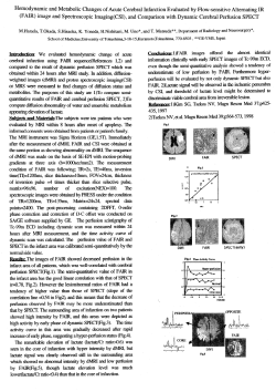


© Copyright 2026