1. art and entertainment
2. books and literature
3. reference books

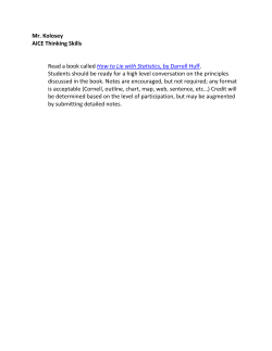
ECG Denoising by Dictionary Learning
Olivier Laligant
IUT Le Creusot
Anastasia Zakharova
IUT Le Creusot
12 rue de la Fonderie
71200 France
[email protected]
[email protected]
Christophe Stolz
IUT Le Creusot
[email protected]
Abstract
In this paper we propose an algorithm for ECG denoising based on dictionary learning. The experimental results
are compared to the results of the algorithm based on sparse
2-dimensional separable transform with overcomplete dictionaries. Besides, we study the behavior of the algorithm
on the signals with natural noise.
1. Introduction
An important issue in the diagnosis of cardiovascular
diseases is the analysis of the form of ECG signals. These
signals are usually damaged with noise coming from different sources, therefore to identify a waveform or to fix an
anomaly we need to remove noise.
The most important features of the signal which should
be preserved while denoising are the form of QRS complex and time localization of peaks since they contain the
key information about the signal. Among the most popular
approaches one could mention wavelet denoising first proposed by Donoho in [6].
In this paper we will introduce a new algorithm of ECG
denoising based on dictionary learning. That is, we will first
build an overcomplete dictionary adapted to different types
of ECG signals and use it for denoising. We will see that a
dictionary learned on a sufficiently big training set performs
well on different ECG signals. In particular, the denoising
method based on such a dictionary preserves the form of
QRS complex that allows us to recognize an anomaly. We
show that the proposed algorithm outperforms the algorithm
of ECG denoising by sparse 2d-separable transform introduced in [1].
2. Sparse decompositions with overcomplete
dictionaries
The idea of compressed sensing is based on an observation that many signals can be well-approximated in a sparse
manner (i.e. with few non-zero coefficients) provided we
have a suitable basis. Such a representation enables us to
perform efficiently the analysis of a signal: it suffices to
take a small number of non-adaptive (not depending on the
given signal) measurements in a right basis instead of measuring all the signal. That’s why sparse representations are
widely used for different signal processing tasks such as
reconstruction, denoising, classification, compression. A
nice overview of theoretical and numerical aspects of compressed sensing could be found in [9] or in [4] while the
basic principles were introduced in [5].
Let us consider a signal x ∈ Rm and a dictionary D =
[d1 , . . . , dk ] ∈ Rm×k (the case k > m is allowed, meaning
that the dictionary is overcomplete). If we define
∥α∥0 = |supp(α)|
(1)
(we use a conventional notation ∥ · ∥0 though it is not a
norm), then the decomposition coefficients are found by
solving the l0 -minimization problem
min ∥α∥0 s.t. Dα = x,
(2)
i.e., we are looking for the sparsest decomposition in D (the
case of an overcomplete dictionary corresponds to the case
of underdefined system of linear equations and we choose
among them the sparsest one). However, since this problem is non-convex and non-smooth, and was shown to be
N P -hard in general, it is usually replaced by a convex minimization problem referred to as l1 -minimization problem
(known also under the name of basis pursuit):
min ∥α∥1 s.t. Dα = x,
(3)
∑k
where ∥α∥1 =
i=1 |αi |. If 2 has a sparse solution, it
will be the solution of 3 as well ([5]). Indeed, the realvalued case of 3 is equivalent to a linear programming task,
so standard numerical methods could be applied to solve it,
although more performing methods also exist.
A common denoising method is to transform the signal
using a fixed (complete or overcomplete) dictionary, to perform shrinkage using either hard or soft thresholding and
finally to apply inverse transform. For example, Ghaffari
et al. [1] used two-dimensional overcomplete DCT and
DCT+Wavelet dictionaries for ECG denoising.
It appears that the choice of the dictionary is crucial for
the performance of a denoising method. However it is not
always clear which dictionary to choose. Usually several
dictionaries are compared ’manually’ and the one giving
the sparsest representation is chosen. To avoid this, we will
train our dictionary so that the representation of typical signals is as sparse as possible.
which is convex with respect to each of two variables D
and α when the other one is fixed. The technique used by
Lee et al. [7] for solving this problem consists in alternating
between two variables: while one of them is minimized, the
other one is fixed.
We will use the algorithm of online dictionary learning
proposed by Mairal et al. [8]. That is, we use the method of
block-coordinate descent with warm restarts described by
Bertsekas [3] to update the dictionary and LARS-Lasso algorithm ([2]) to optimize the value of α. The advantage of
block-coordinate descent is that it is parameter free and does
not require much memory for storage, since the columns of
D are modified sequentially. Furthermore, while calculating Di the previous iteration Di−1 could be used as warm
restart. The motivation for this comes from the fact that
2.1. Dictionary learning
Let D0 ∈ Rm×k be the initial dictionary, X =
[x1 , . . . , xn ] ∈ Rm×n be the training set. The number of
signals n in the training set is significantly larger than the
signal dimension m. The size of the dictionary k is equal
or bigger than m. Generally, k ≪ n. We are looking for a
dictionary D which will provide us a good sparse approximation for the signals from the training set. To do this, we
optimize the cost function
1∑
l(xi , D),
n i=1
1∑
fˆi (x, Di ) =
i j=1
i
(
1
∥xi − Di αi ∥22 + λ∥αi ∥1
2
n
f (D) =
(4)
where l(x, D) is a loss function which is small if the representation of x is sparse in D. Following Lee et al. [7],
we define function l(x, D) as the minimal value of l1 minimization problem:
l(x, D) = min
α∈Rk
1
∥x − Dα∥22 + λ∥α∥1
2
(5)
with λ being a regularization parameter. It’s well known
that the solution α of 5 is sparse.
It is not yet clear how the sparsity of x depends on the
value of the parameter λ. We nevertheless choose a positive
regularization parameter to avoid overfitting for the training
set which can lead to a bad representation of test signals.
In order that the values of α were not arbitrarily small
we will put an additional constraint on the l2 -norms of the
vectors in D. Let C be the convex set of matrices verifying
this constraint:
C = {D ∈ Rm×k s.t. ∀j = 1, . . . , k, dTj dj ≤ 1}.
(6)
To find the dictionary we solve a joint optimization problem
min
D∈C,α∈Rk
1
∥x − Dα∥22 + λ∥α∥1 ,
2
(7)
converges almost surely [8].
2.2. Algorithm
)
(8)
Dictionary Learning - Preprocessing Step
for i=1 to n
1. Using LARS-Lasso optimization method, compute
αi = arg min 12 ∥xi − Di−1 α∥22 + λ∥α∥1
25
Output SNR
Input: [x1 , . . . , xn ] ∈ Rm×n - training set,
D0 ∈ Rm×k - initial dictionary
λ - regularization parameter
30
20
15
10
α∈Rk
2. Compute Di using Di−1 as warm restart:
i (
)
∑
1
2
Di = arg min 1i
2 ∥xi − Dαi ∥2 + λ∥α∥1
D∈C
Trained dictionary
2d overcomplete dictionary
5
0
5
10
15
Input SNR
j=1
end
Figure 1. Comparison of denoising methods in terms of SNR
Output: D = Dn ∈ Rm×k - trained dictionary
sampling rate of given signals: the signal period contains
about 200 samples (since it depends on a patient it varies
from signal to another). The training of the dictionary is
more efficient if the size of the signals in the training set is
Input: x ∈ RN - signal damaged with noise,
comparable to the length of the period. Besides, taking m
D ∈ Rm×k - trained dictionary
reasonably big accelerates the algorithm.
λ - regularization parameter
As a test set we use signals from the MIT-BIH Arrythmia
1. Extract the segments of length m from the signal
database which is claimed to be a representative selection of
(the overlap of the segments does not exceed ⌊m/2⌋ samples) the variety of waveforms and artifacts that occur in routine
and concatenate them so that we get a matrix X with m lines clinical use.
2. Decompose each column of the matrix X in D
(using Lasso optimization technique)
3.1. Case of added Gaussian noise
3. Calculate the inverse transform
Taking a signal from the test set, we add to it randomly
4. Put the segments back in their original places;
generated
Gaussian noise with different variances. Then
in the overlap domain, calculate the mean of two signals
the denoising is performed and output SNR is calculated
for the method based on dictionary learning and for the 2Output: xr - denoised signal
dimensional sparse separable method [1]. The results presented in Fig.1 are average results of thirteen test signals.
3. Experimental results
As one can see from it, the denoising method based on dicLet us now examine the performance of the proposed altionary learning outperforms the 2-dimensional sparse sepgorithm. This section consists of two parts. First, we add
arable method.
a randomly generated white Gaussian noise to a signal and
Let us mention that in [1] the 2-dimensional sparse sepapply the denoising algorithm. Then we compare the result
arable algorithm is compared to the methods of soft threshwith the original signal by the means of SNR (here we use
olding [6] and extended Kalman smoother filtering [10] in
∥x∥
the usual definition of SNR in = 20 log( ∥n∥
) for input SNR
terms of SNR and it is experimentally shown that it outper∥x∥
forms both of them (the MIT-BIH Normal Sinus Rhythm
and SNR out = 20 log( ∥x−xr ∥ ) for output SNR, where by
Database was used for simulations).
x we denote the original signal, by xr the reconstructed signal, by n added noise).
3.2. Case of natural noise
In the second part we take noisy signals and apply the
denoising algorithm.
For this simulation we take a signal from the MIT-BIH
Arrythmia Database that contains a noisy segment. In this
To learn the dictionary we use the database of ECG
case, we have no idea of the form of the original signal.
records obtained by the Creusot - Montceau-les-Mines hosHowever, since ECG signal is almost periodical it is reapital. We choose 14 signals taking a segment of 1000 samsonable to suppose that its denoised version might look like
ples from each of them in such a way that they represent the
the previous segment of the same signal. Using the same
variety of clinically important phenomena. The training set
parameters as in the previous subsection we perform the deis then formed by all the segments of length m = 128 of
noising using the learned dictionary.
each of these signals. The choice of m is motivated by the
Signal Denoising
Initial signal
Initial signal with Gaussian noise
1
1
0
0
−1
−1
0
500 1000 1500 2000 2500
Denoising by dictionary learning
0
Denoising by sparse 2d transform
1
1
0
0
−1
−1
0
500 1000 1500 2000 2500
500 1000 1500 2000 2500
0
500 1000 1500 2000 2500
Figure 2. Performance of denoising algorithms on the signal with added Gaussian noise
The results of the simulation are presented on 3. We see
that the form of the denoised signal is very similar to the one
of the segment of the same signal. For completeness, we
also give the result of denoising by using the 2-dimensional
sparse separable method.
3.3. Conclusion
We proposed the denoising algorithm based on learned
dictionary. The simulation results show that the method
performs well on noisy signals and outperforms the 2dimensional sparse separable method for the signals with
added Gaussian noise.
References
[1] M. B.-Z. C. J. A. Ghaffari, H. Palangi. Ecg denoising and
compression by sparse 2d separable transform with overcomplete mixed dictionaries. 2010.
[2] I. J. B. Efron, T. Hastie and R. Tibshirani. Least angle regression. Annals of Statistics, 32.
[3] D. Bertsekas. Nonlinear programming. Athena Scientific
Belmont.
[4] E. Cand`es and M. Wakin. An introduction to compressive
sampling. IEEE Signal Processing Magazine, 25.
[5] D. Donoho. Compressed sensing. IEEE Trans. on Information Theory, 52.
[6] D. Donoho. Denoising by soft-thresholding. IEEE Trans. on
Information Theory, 41:613–627, 1995.
[7] R. R. H. Lee, A. Battle and A. Ng. Efficient sparse coding
algorithms. Advances in Neural Information Processing Systems, 19:801–808, 2007.
[8] J. P.-G. S. J. Mairal, F. Bach. Online learning for matrix factorization and sparse coding. Journal of Machine Learning
Research, 11:19–60, 2010.
[9] M.Fornasier and H. Rauhut. Compressive sensing, 2011.
Chapter in Part 2 of the ”Handbook of Mathematical Methods in Imaging” (O. Scherzer Ed.), Springer, 2011.
[10] C. J. R. Sameni, M.B. Shamsollahi and G. Clifford. A nonlinear bayesian filtering framework for ecg denoising. IEEE
Trans. on Biomedical Engineering, 54:2172–2185, 1007.
Noisy segment
Denoising by dictionary learning
1
1
0.5
0.5
0
0
−0.5
−0.5
−1
−1
500
600
700
800
500
Similar segment without noise
1
0.5
0.5
0
0
−0.5
−0.5
−1
−1
300
400
500
700
800
Denoising by sparse 2d separable transform
1
200
600
500
600
700
800
Figure 3. Performance of the denoising algorithm on the signal with natural noise