1. science
2. mathematics
3. geometry

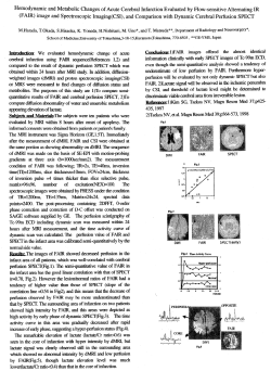
PHYSICAL REVIEW E
VOLUME 57, NUMBER 5
MAY 1998
Karhunen-Loève analysis of spatiotemporal flame patterns
Antonio Palacios,1,2,* Gemunu H. Gunaratne,1,† Michael Gorman,1,‡ and Kay A. Robbins3,§
1
Department of Physics, The University of Houston, Houston, Texas 77204
Department of Mathematics, The University of Houston, Houston, Texas 77204
3
Division of Computer Science, University of Texas at San Antonio, San Antonio, Texas 78249
~Received 17 June 1997; revised manuscript received 26 January 1998!
2
The ability of Karhunen-Loève ~KL! decomposition to identify, extract, and separate the spatial features that
characterize a spatiotemporal system is demonstrated using video images from a combustion experiment and
nonstationary states from a phenomenological model. Cellular flames on a circular porous plug burner exhibit
a variety of stationary and nonstationary patterns. KL decomposition is used to analyze the spatiotemporal
dynamics of four experimental states: one- and two-cell rotating states, two counterrotating rings, a standingwave state, and two one-cell rotating states from numerical simulations of a phenomenological model designed
to study pattern formation in a circular domain. The KL technique optimally captures the dynamics of the
states by producing a linear subspace on which the reconstructed dynamics has a minimum truncation error. It
identifies the dominant spatial structures whose coupling produces the observed patterns and distinguishes
between uniform and nonuniform rotational motion. The implementation of this technique using video images
as input is explained and the implications of symmetry in interpreting the KL analysis of the dynamics are
described. @S1063-651X~98!07105-0#
PACS number~s!: 82.40.Ra, 82.40.Py, 11.30.Qc, 82.20.Mj
I. INTRODUCTION
Cellular flames form ordered patterns of concentric rings
of cells when stabilized on a circular porous plug burner at
low pressure. As the control parameters are varied,
symmetry-breaking bifurcations are observed to dynamic
states in which the cells move, exhibiting both periodic and
complex dynamics. This paper demonstrates the ability of
Karhunen-Loève ~KL! decomposition to identify the dominant spatial structures of nonstationary flame patterns and to
characterize the time dependence of the pattern of evolution.
The spatial modes and their time evolution are extracted directly from two-dimensional video images produced in the
experiment, in contrast to applications that use onedimensional spatial information or that rely on time series at
isolated points.
In an attempt to quantify flame dynamics using KL decomposition, a pulsating single-cell state found in methaneair flames was considered by Stone et al. @1#. A distinctive
feature of this state is the coexistence of time-periodic pulsations with spatial chaotic motion in the orientation of the
cell. To unravel the complexity, Stone et al. applied KL decomposition to a data set consisting of the cell boundaries.
They found that the motion of the boundaries could be described by three KL eigenvectors. The reconstruction with
these three eigenvectors resembled the original twodimensional motion, and the long-term evolution indicated
the presence of a limit cycle in phase space. Insight into
multiple-ring formation was obtained using synthetic data to
mimic the spatial structure of the cells and their motion.
*Electronic address: [email protected]
†
Electronic address: [email protected]
Electronic address: [email protected]
§
Electronic address: [email protected]
‡
1063-651X/98/57~5!/5958~14!/$15.00
57
In subsequent work, a boundary extraction procedure was
developed and implemented to study several nonstationary
states with multiple rings @2#. Four representative cases were
studied: an outer rotating ring of cells concentric with an
almost fixed inner ring, a single rotating ring surrounding
one central cell, a ratcheting motion described by a periodic
locking-unlocking mechanism of two rotating rings, and an
intermittent state characterized by recurrent appearances of
ordered patterns. The Karhunen-Loève analysis using boundary extraction revealed the presence of two intrinsic types of
dynamics: one describing the large-scale motion of the rings
and one representing the small-scale oscillatory motion of
the cells. The rings appeared to be weakly coupled and the
temporal evolution of the modes was used to describe the
long-term evolution of the patterns.
While the analysis of cell boundaries was useful for describing the overall motion of the patterns, some important
issues remain unresolved. There was little indication as to
how the patterns emerge and whether the nonstationary
states represent cases of uniform or nonuniform motion. Another point of interest is the study of more complicated
states. Since the boundary extraction procedure is only applicable to states where the number of cells remains constant,
the analysis cannot be used to describe states where cells
merge and split. Many of these limitations arise because cell
boundary extraction is strictly a one-dimensional technique
that fails to recognize and identify the role played by the
two-dimensional character of the spatial dynamics. However,
the investigation of the boundary motion offers the advantage of requiring less computational time and memory than a
two-dimensional analysis based directly on the images.
In a recent paper @3# we presented a phenomenological
model that described general characteristics of pattern formation in a circular domain. Certain dynamical states of the
experiment were reproduced in the model, and KL decomposition was used to demonstrate the similarity between the
5958
© 1998 The American Physical Society
57
KARHUNEN-LOÈVE ANALYSIS OF SPATIOTEMPORAL . . .
5959
experimental states and the numerical results. In this paper
we focus on the implementation of KL decomposition for the
video image data, we relate the symmetry of the dynamical
states to the symmetries of the KL eigenfunctions, and we
amplify our analysis of each dynamical state by presenting
phase-space trajectories of the KL coefficients.
KL decomposition optimally captures the behavior of
two-dimensional flame patterns by producing a linear subspace on which the reconstructed dynamics has a minimum
truncation error. Certain properties of this subspace can be
used to explain the symmetries of the cells in nonstationary
states @4#. The structure of the KL eigenfunctions is used to
explain the formation of the patterns and to differentiate between uniform and nonuniform motion.
The experimental system is described in Sec. II. The
mathematical development of KL decomposition relevant to
this study is presented in Sec. III. Important aspects related
to the implementation of the KL decomposition with video
images are discussed and the implications of symmetry are
emphasized. Representative cases of experimental flame patterns and simulations from a phenomenological model are
analyzed in Sec. IV. The results are discussed in Sec. V.
II. COMBUSTION EXPERIMENT
The experimental system consists of a circular porous
plug burner that burns premixed gases inside a low pressure
~0.3–0.5 atm! combustion chamber. Mixtures of isobutane
and air were used for the experiments described in this paper.
The pressure, flow rate, and fuel-to-oxidizer ratio are controlled to within 0.1%. A steady uniform flame appears as a
circular luminous disk, 5.62 cm in diameter and 0.5 mm
thick. The flame front forms roughly 5 mm above the surface
of the burner.
A Dage-MTI charge coupled device camera, mounted
vertically on top of the combustion chamber, is used to
record the evolution of the flame front. A distinctive feature
of premixed flames, as a system exhibiting spatiotemporal
dynamics, is that an important dynamical variable is the local
temperature which can be measured using the emitted chemiluminescence from the flame front. The spatial and temporal
resolution, the time interval, and the dynamic range are
limited only by the recording device. Images of 6403480
pixel resolution, taken at 1/30-sec intervals with a 7-bit dynamic range, are typical for dynamics recorded on S-VHS
video tape.
Upon changes of parameters ~type of fuel, pressure, total
flow, and equivalence ratio! the flame front forms ordered
patterns of concentric rings of cells. Brighter cells correspond to hotter regions on the burner. They are separated by
darker regions corresponding to cusps and folds that extend
an additional 5 mm away from the surface of the burner. As
the parameters are varied, the O~2! symmetric uniform state
bifurcates to other stationary states or to dynamical states
with less spatiotemporal symmetry @5#. In the former case,
new ring structures emerge with different spatial symmetries
and various numbers of cells. In this paper we consider four
nonstationary states: a single rotating cell, two rotating cells,
two counterrotating rings, and a standing wave of two cells.
Figure 1 shows four sequential frames of videotape from
these states. Each state was reached by an abrupt change in
FIG. 1. Four sequential frames of videotape of four different
experimental cellular flame states: ~a! a single rotating cell, ~b! two
rotating cells, ~c! counterrotating rings, and ~d! a standing wave
between two cells.
the control parameters during a coarse survey of parameter
space.
III. KARHUNEN-LOÈVE DECOMPOSITION
Karhunen-Loève decomposition is a well-known technique for determining an optimal basis for a data set @6–10#.
This section reviews the definitions and properties of KL
decomposition relevant to this paper and discusses how the
method can be applied to image data in order to separate
spatial and temporal behavior.
Consider a sequence of observations represented by the
scalar functions u(x,t i ),i51, . . . ,M . The functions u are
assumed to be L 2 on a domain D that is a bounded subset of
R n . The functions are parametrized by t i , which represents
time in this application. The ~time! average of the sequence,
M
defined as ū(x)5 ^ u(x,t i ) & 5(1/M ) ( i51
u(x,t i ), is assumed
to be zero. The KL decomposition extracts time-independent
orthonormal basis functions F k (x) and time-dependent orthonormal amplitude coefficients a k (t i ) such that the reconstruction
u ~ x,t i ! 5 ( a k ~ t i ! F k ~ x! ,
i51, . . . ,M ,
~3.1!
is optimal in the sense that the average least-squares truncation error
« N5
KI
(
k51
IL
2
N
u ~ x,t i ! 2
a k ~ t i ! F k ~ x!
~3.2!
5960
PALACIOS, GUNARATNE, GORMAN, AND ROBBINS
is always a minimum for any given number N of basis functions over all possible sets of orthogonal functions.
The functions F k (x), called empirical eigenfunctions, coherent structures, or KL modes, are the eigenvectors of the
two-point spatial correlation function
M
r ~ x,y! 5
1
u ~ x,t i ! u T ~ y,t i ! .
M i51
(
~3.3!
A. Application to image data
KL decomposition can be generally applied to find an
optimal basis for a data set. To separate the spatial and the
time behavior for a physical system, each point in the data
set should represent an observation of the spatial state of the
system at a particular time. KL decomposition is applied to
the observations to find an optimal basis for the spatial observations. The data set is projected on the resulting KL basis
functions to obtain the time behavior in much the same way
as normal mode expansions are used for partial differential
equations. The KL technique is based purely on the observations and thus has the advantage of not requiring knowledge
of an underlying model equation or normal modes.
In practice the state of a numerical model is only available
at discrete spatial grid points and so the observations that
form the data set are vectors rather than continuous functions. In other words, D5(x 1 ,x 2 , . . . ,x N ), where x j is the
jth grid point and u(x,t i ) is the vector ui
5„u(x 1 ,t i ),u(x 2 ,t i ), . . . ,u(x N ,t i )…T .
Experimental data also undergoes a discretization process
when it is acquired for processing. In the case of the combustion experiment, images of the flame front were digitized
to obtain the observations at different times. Each image is a
w3h5N array of pixels. A pixel is a scalar value in the
interval @0,255#. An image can be converted to a vector by
ordering the pixel values in row major form @e.g., the pixel
( j,k) in the image is stored in the position n5 j3w1k in
the vector#.
B. Method of snapshots
A popular technique for finding the eigenvectors of Eq.
~3.3! is the method of snapshots developed by Sirovich @10#.
It was introduced as an efficient method when the resolution
of the spatial domain (N) is higher than the number of observations (M ). The method of snapshots is based on the fact
that the data vectors ui and the eigenvectors F k span the
same linear space ~see @6,10# for details!. This implies that
the eigenvectors can be written as a linear combination of the
data vectors
M
F k5
( v ki ui .
i51
~3.4!
After substitution in the eigenvalue problem r(x,y)F(y)
5lF(x), the coefficients v ki are obtained from the solution
of
Cv5lv,
~3.5!
57
where vk5( v k1 , . . . , v kM ) is the kth eigenvector of Eq. ~3.5!
and C is a symmetric M 3M matrix defined by
@ c i j # 5(1/M )(ui ,u j ), where ( , ) denotes the standard
vector inner product (ui ,u j )5u(x 1 ,t i )u(x 1 ,t j )1•••
1u(x N ,t i )u(x N ,t j ). In this way an N3N eigenvalue problem @the eigenvectors of Eq. ~3.3!# is reduced to computing
the eigenvectors of an M 3M matrix, a preferable task if N
@M . Throughout the remaining of this work, M will denote
the number of measurements of a laboratory or numerical
experiment and N will represent the maximum number of
KL eigenfunctions employed in a particular reconstruction of
an experiment. The results presented in Sec. IV were obtained with an implementation of the method of snapshots.
C. Properties of KL decomposition
Since the kernel is Hermitian r(x,y)5r * (y,x), it admits,
according to the Riesz theorem @11#, a diagonal decomposition of the form
N
r ~ x,y! 5
(
k51
l k F k ~ x! F k* ~ y! .
~3.6!
This fact is particularly useful when finding the KL modes
analytically. They can be read off from the diagonal decomposition ~3.6!.
The temporal coefficients a k (t i ) are calculated by projecting the data set on each of the eigenfunctions
a k ~ t i ! 5„u ~ x,t i ! ,F k ~ x! …,
i51, . . . ,M .
~3.7!
It can be shown that both temporal coefficients and eigenfunctions are uncorrelated in time and space, respectively
@6,10#.
Proposition 1. The KL modes $ F k (x) % with corresponding temporal coefficients $ a k (t i ) % satisfy the following orthogonality properties: ~i! F *j (x)F k (x)5 d jk and ~ii!
^ a j (t i )a *k (t i ) & 5 d jk l j , where d jk represents the Kronecker
delta function.
Property ~ii! is obtained when the terms in the diagonal
decomposition ~3.6! are compared with the expression
r(x,y)5 ( ^ a j (t i )a *
k (t i ) & F j (x)F *
k (y). The non-negative and
self-adjoint properties of r(x,y) imply that all eigenvalues
are non-negative and can be ordered accordingly:
l 1 >l 2 >•••>0. Statistically speaking, l k represents the
variance of the data set in the direction of the corresponding
KL mode, F k (x). In physical terms, if u represents a component of a velocity field, then l k measures the amount of
kinetic energy captured by the respective KL mode F k (x). In
this sense, the energy measures the contribution of each
mode to the overall dynamics.
Definition 1. The total energy captured in a KarhunenLoève decomposition of a numerical or experimental data set
is defined as the sum of all eigenvalues
N
E5
(
k51
lk .
~3.8!
The relative energy captured by the kth mode, E k is defined
by
57
KARHUNEN-LOÈVE ANALYSIS OF SPATIOTEMPORAL . . .
E k5
lk
N
(
~3.9!
.
lj
j51
The cumulative sum of relative energies ( E k approaches one
as the number of modes in the reconstruction increases.
Spatiotemporal systems are capable of producing different
kinds of behavior including periodic, quasiperiodic, and nonperiodic motion in space and time. In some cases, the KL
decompositions of qualitatively different states may produce
seemingly similar spectra. However, the decomposition can
still be used to differentiate between different solutions. One
possibility is to apply the KL decomposition to the state of
interest and then use the KL energy spectrum to calculate the
entropy of the data set. The entropy is a measure of order or
disorder and provides an objective way of classifying the
complexity in experimental or numerical data.
Definition 2. The entropy E of a KL decomposed data set
u can be calculated from its energy spectrum according to
E~ u ! 52 lim
N→`
1
lnN
N
(
k51
E k lnE k ,
~3.10!
where lnN is a normalization factor that allows comparisons
between different data sets.
The entropy, as defined by Eq. ~3.10!, measures the energy distribution among the modes in the KL spectra and
varies between 0 and 1, as the number of modes increases.
The entropy is low when the energy is concentrated in a few
modes. A zero entropy indicates that only one eigenfunction,
with maximal energy E 1 51, is needed to reproduce the dynamics. The entropy approaches 1 when the energy spreads
across a large number of modes, indicating complex behavior.
Equation ~3.2! states that Karhunen-Loève decomposition
produces a basis that minimizes the least-squares truncation
error. This property can also be stated in terms of the energy
captured by the KL modes.
Proposition 2. Let $ a k (t i ),F k (x) % be the KL basis pairs
obtained from a scalar field u(x,t i ) satisfying Eqs. ~3.1!,
~3.6!, and ~3.7!. Let $ b k (t i ),C k (x) % be any arbitrary orthonormal basis pair satisfying Eq. ~3.1!. The KL basis is optimal in the sense that the total cumulative energy captured by
the sequence $ a k (t i ),F k (x) % is always greater than or equal
to the total cumulative energy captured by $ b k (t i ),C k (x) %
provided the number of eigenfunctions ~respecting their ordering from most to least energetic! employed is the same.
Formally
N
(
k51
N
E k5
(
k51
N
^ a k ~ t i ! a *k ~ t i ! & 5
(
k51
N
l k>
(
k51
^ b k ~ t i ! b *k ~ t i ! & .
~3.11!
D. Consequences of symmetry
One motivation for applying KL decomposition is to obtain information about the long-term behavior of the system.
Suppose that this behavior is captured by an attractor, denoted by A ~see @12# for a precise definition!. Assume also
that scalar measurements of the system g(x,t i ), i
5961
51, . . . ,M , are provided. In practice, one must first comM
pute the average ḡ(x)5(1/M ) ( i51
g(x,t i ) in order to produce a new set of measurements u(x,t i )5g(x,t i )2ḡ(x)
with zero average. Let G denote the group of symmetries of
the system of interest. The symmetries of the attractor form a
subgroup of G defined by
G ~ A! 5 $ g PG u g A5A % .
~3.12!
The critical observation is that the symmetries of the attractor A appear as symmetries of the time average ḡ(x) independently of the symmetries of the instantaneous scalar field
g(x,t i ) @14#. Unfortunately, the converse is not always true.
The symmetries of the time average do not necessarily reflect
the symmetries of the underlying attractor. Furthermore, the
KL decomposition satisfies the following symmetry properties.
Proposition 3. Let $ F(x) % be the KL eigenfunctions satisfying the eigenvalue problem ^ u(x,t)u * (y,t) & F(y)
5lF(x). Then ~i! ^ g u(x,t) g u * (y,t) & g F(y)5l @ g F(x) #
for all g PG, ~ii! ^ s u(x,t) s u * (y,t) & 5 ^ u(x,t)u * (y,t) & for
all s PG (A) , and ~iii! ^ u(x,t)u * (y,t) & s F(y)5l @ s F(x) #
for all s PG (A) .
Property ~i! establishes that the eigenfunctions in the KL
decomposition of g u(x,t) are those of u(x,t) under the action of g . This property explains the observation that the KL
decomposition of a periodic data set is not unique. If F(x) is
an eigenfunction, so is g F(x) for all g PG. Which one is
then chosen? In the case of experimental or computational
data, the answer depends on how the data are collected. Performing the decomposition with different initial conditions
may produce a rotated version of F(x). Nevertheless, the
important point is to realize that they are all symmetrically
related. Properties ~ii! and ~iii! indicate that the KL kernel
and its eigenvectors have at least the same symmetries as the
attractor.
E. Traveling waves and KL decomposition
Consider a periodic traveling wave represented by a periodic function in the form u(x,t)5 f (x2ct), where c denotes
the speed of the wave. As noted in @13#, the KL decomposition coincides with the Fourier decomposition
`
f ~ x2ct ! 5
(
k52`
c k e 2ik p ~ x2ct ! .
~3.13!
The alternative form
`
f ~ x2ct ! 5
( Aa 2k 1b 2k @ cos~ k p ct1 a k ! sin~ k p x !
k50
2sin~ k p ct1 a k ! cos~ k p x !#
~3.14!
shows the KL modes explicitly. Here c k 5(a k 1b k i)/2 are
the Fourier coefficients of f (x2ct) with phase a k
5tan21 (2a k /b k ). The KL modes can be written as ordered
pairs of the form $ F 2k21 ,F 2k % 5 $ cos(kpx),sin(kpx)%. The
traveling wave is produced by the coupling of pairs of modes
that contain the same energy and maintain a constant relative
phase.
PALACIOS, GUNARATNE, GORMAN, AND ROBBINS
5962
57
By analogy with pure periodic traveling waves, adjacent
KL modes with the same symmetry and equivalent energy
may be associated with traveling-wave solutions. Such adjacent modes are called coupling modes.
Definition 3. Let u(x,t i )5 ( Nk51 a k (t i )F k (x), i
51, . . . ,M , represent the KL decomposition of a data set.
The relative phase of KL eigenfunctions m and n, mÞn, is
defined by
S
f mn ~ t i ! 5tan21 2
D
a n~ t i !
.
a m~ t i !
~3.15!
The relative phase f mn between KL modes F m and F n has
the following geometric interpretation. If the temporal coefficients a m (t i ) and a n (t i ) are represented by a point in a
phase plane plot, then f mn (t i ) are observations of the angular displacement of the plotted point as it moves in the phase
plane. A relative phase between coupling modes that is linear
indicates an underlying traveling-wave solution that is moving uniformly. Similarly, a nonlinear relative phase indicates
a modulated traveling wave or perhaps more complicated
behavior.
In the traveling wave described by Eq. ~3.14!, we find that
f (2k21)(2k) (t)5k p ct1 a k ~mod p ) is the relative phase between coupling modes. Observe that this relative phase
f (2k21)(2k) is not uniquely defined. An alternative expression
`
f ~ x2ct ! 5
( Aa 2k 1b 2k @ cos~ k p ct ! sin~ k p x1 a k !
k50
2sin~ k p ct ! cos~ k p x1 a k !#
~3.16!
shows that f (2k21)(2k) (t)5k p ct ~mod p! is also possible.
From the viewpoint of symmetry, each pair of KL modes
$ cos(kpx),sin(kpx)% forms an irreducible subspace for the
representation of the traveling wave. Any left-right shift of
these modes, with temporal coefficients shifted accordingly,
can also be used as a KL basis.
FIG. 2. Examples of one-cell states from the experiment rotating
~a! clockwise and ~b! counterclockwise.
tions of the underlying system. It has been demonstrated
@17,18# that in one-dimensional interfaces, traveling cells appear as a result of a parity breaking in which the cells lose
their left-right symmetry. A manifestation of parity breaking
in a two-dimensional system is demonstrated by these rotating cellular flame states @19#. Figure 2~a! shows an experimental state in which a single cell executes clockwise rotation, while Fig. 2~b! shows a related state in which a single
cell rotates in the counterclockwise direction.
1. One-cell rotating state: Experiment
The single rotating cell state shown in Fig. 2~a! was chosen for the KL analysis. Sixty frames, digitized at a rate of 30
frames/sec, contain about seven complete revolutions of the
cell. Figure 3~a! shows some instantaneous snapshots, Fig.
3~b! shows the eigenfunctions extracted by the KL decomposition, and Fig. 3~c! shows the KL reconstructions based
on the corresponding eigenfunctions. The top snapshot in
IV. RESULTS
A. Computational details
For each of the flame patterns analyzed in this section, a
representative sequence of video images was digitized. Depending on the speed of the motion, a capturing rate of 15 or
30 frames per second was employed. Sufficient frames
(;200) for each state were captured to obtain a well-defined
time-average pattern and several full multiples of the period.
Each image frame was then scaled to 64364 pixels and converted from an audio-video interlace movie format to a
stream of intensity values ranging from 0 to 255. The
KLTOOL software package @15# was used to perform an interactive KL decomposition. For each case analyzed, a computer animation comparing reconstructions from different
KL modes can be found on the World Wide Web @16#.
B. Single-ring rotating states
Ordered states of concentric rings of cells bifurcate to
states in which entire rings of cells rotate either clockwise or
counterclockwise @5#. Rotating states, which are typically
found in isobutane-air flames, represent traveling-wave solu-
FIG. 3. A KL decomposition of a rotating one-cell state from
the experiment: ~a! four instantaneous snapshots showing a clockwise rotating cell; ~b! the time average of the data set appears at the
top, followed ~from left-to-right and top-to-bottom! by the four
most energetic modes F 1 , F 2 , F 3 , and F 4 ; and ~c! the reconstruction of the dynamics using the four most energetic KL modes.
57
KARHUNEN-LOÈVE ANALYSIS OF SPATIOTEMPORAL . . .
5963
FIG. 4. Energy spectrum for the KL decomposition of the rotating one-cell state of Fig. 3~a!.
Fig. 3~b! is the time average of the images. The four most
energetic KL modes F 1 , F 2 , F 3 , and F 4 are depicted below
the time average ~from left to right and top to bottom, respectively! in Fig. 3~b!. The KL reconstruction using the first
two modes F 1 and F 2 captures the rotation of the cell. The
reconstruction with the first four KL modes @Fig. 3~c!# further improves the representation of the motion and shape of
the cell. The similarity to the original state is clearly visible.
The KL energy spectra ~Fig. 4! shows that 75% of the
total energy is captured by the first four modes. The energy
is almost equally distributed between F 1 and F 2 , indicating
that they form a coupling pair. Similarly, F 3 and F 4 also
form a coupling pair. The remaining modes capture less energy ~25%! and contain high-dimensional information. A
75% cutoff between low-dimensional and high-dimensional
dynamics has also been observed in the KL analysis of other
experiments @20#.
The long-term motion of a cell can be understood from
the temporal coefficients a 1 (t), a 2 (t), a 3 (t), and a 4 (t) associated with the most energetic KL modes ~Fig. 5!. The sinusoidal nature of these projections is evidenced by their time
plots @Figs. 5~a! and 5~b!#. The $ a 1 (t),a 2 (t) % pair forms a
traveling wave, which results in a uniform rotation of 3.3
rev/sec. The $ a 3 (t),a 4 (t) % pair oscillates at twice the frequency of the first pair @compare Fig. 5~a! with Fig. 5~b!#,
indicating their role as a higher spatial harmonic in defining
the cell shape. This phenomenon can be understood from the
spatial symmetries of the two pairs of modes. F 1 and F 2
have ~approximately! D 1 symmetry, meaning that they will
return to their original pattern in one complete rotation. In
contrast, F 3 and F 4 have D 2 symmetry. They return to their
original pattern in half a revolution. In general, the primary
spatial harmonic of a periodic pattern with D n symmetry will
have D 2n symmetry. The harmonic only has to rotate half as
far as the original mode to reestablish the original pattern.
Figure 6~a! shows the behavior of f 12 , the relative phase
between the first pair of KL modes. The nearly linear behavior of the relative phase indicates that the cell is rotating
uniformly.
The SO~2! or O~2! symmetry of the time average in Fig.
3~b! @on the plane SO~2! and O~2! symmetries cannot be
distinguished# reflects the symmetry of the burner, even
though none of the instantaneous snapshots of Fig. 3~a! has
FIG. 5. Temporal coefficients for the four most energetic modes
in the KL decomposition of a single rotating cell shown in Fig. 3:
~a! time plots of a 1 (t) and a 2 (t) and ~b! time plots of a 3 (t) and
a 4 (t).
FIG. 6. Behavior of the relative phase f 12(t) for the one-cell
rotating state from the experiment.
5964
PALACIOS, GUNARATNE, GORMAN, AND ROBBINS
57
this symmetry. Each of the pairs of KL modes $ F 1 ,F 2 % and
$ F 3 ,F 4 % forms an irreducible subspace @4# under the action
of the symmetries of the system, G5O(2)3S 1 for the circular burner. S 1 is the circle group that accounts for the
temporal phase-shift symmetries of periodic states. The invariance of these subspaces implies that if a cellular state has
certain symmetries at one instant of time, then it must have
the same symmetries at all times. Consequently, any cellular
state with a reflectional symmetry must have the same symmetry at all times and it therefore cannot rotate.
Also note that based on Proposition 3~i!, these irreducible
subspaces are not unique. The particular subspace representing each symmetry is selected by initial conditions. Once a
particular subspace is chosen, the KL reconstructed dynamics on that subspace corresponds to a unique branch of periodic solutions with group symmetry ( ,G. According to the
equivariant Hopf theorem with O(2)3S 1 symmetry @4#, two
types of periodic states can appear with ( symmetry: rotating waves and standing waves. The one-cell rotating state
and the other states in this section are examples of rotating
waves.
2. One-cell rotating state: Phenomenological model
Numerical simulations of a phenomenological model @3#
that is closely related to flame dynamics have demonstrated
the formation of both stationary and nonstationary states.
These states emerge as a result of symmetry-breaking bifurcations in which several spatial modes couple and compete
for existence. The model describes the evolution of two
coupled, diffusive spatiotemporal fields u(x,t) and v (x,t)
through
u t 5 k 1 ¹ 2 u1 ~ B21 ! u1A 2 v 2 h u 3 2 n 1 ~ ¹u ! 2 ,
v t 5 k 2 ¹ 2 v 2Bu2A 2 v 2 h v 3 2 n 2 ~ ¹ v ! 2 ,
~4.1!
where k 1 and k 2 are the diffusion coefficients of the two
linearly coupled fields. The cubic terms control the growth of
the linearly unstable modes. The nonlinear gradient terms
render the model nonvariational and are similar to the nonlinear term of the Kuramoto-Sivashinsky equation @21,22#,
which is often used to model flame dynamics. In order to
simulate the circular geometry of the experimental burner,
the integration of Eqs. ~4.1! is carried out in polar coordinates over a circular grid of radius R. Small changes in the
radius R can produce qualitatively different flame patterns.
This observation leads us to consider the radius as a distinguished bifurcation parameter.
Figure 7~a! shows four snapshots of a single-cell state
simulated with Eqs. ~4.1! for parameter values ( h 52.0, n 1
50.5, n 2 51.0, k 1 50.2, k 2 52.0, A55.0, B56.8, and R
51.35). It consists of a single cell rotating clockwise that
does not change its shape. The KL decomposition of a complete period produces an O~2! invariant time-average pattern
@Fig. 7~b!# and four KL modes F 1 , F 2 , F 3 , and F 4 ~depicted from left to right and top to bottom, respectively!. A
similar KL spectrum indicates that the first two modes F 1
and F 2 capture about 94% of the energy as compared to
65% ~considering only the first two modes! for the experimental one-cell rotating state shown in Fig. 3~a!. Only two
modes are necessary to reconstruct the dynamics and the
FIG. 7. ~a! Four snapshots of a uniformly rotating one-cell state
produced from simulations of Eqs. ~4.1!, ~b! the time average and
~from left-to-right and top-to-bottom! the four most energetic KL
modes, and ~c! reconstruction of the dynamics using the four most
energetic KL modes.
remaining modes affect other aspects such as cell shape.
Nearly 100% of the energy is captured by the first four
modes. The reconstruction with these four KL modes is
shown in Fig. 7~c!.
The details of the temporal behavior of the cell are extracted from the KL projections. Figure 8~a! shows phase
plots of a 1 (t) vs a 2 (t), a 3 (t) vs a 4 (t), and a 1 (t) vs a 3 (t).
The first pair indicates the uniform rotation of the cell. The
second pair indicates a periodic oscillation at twice the frequency of the dominant pair. The plots of the relative phases
for each pair of KL modes shown in Fig. 8~b! confirm this
relationship.
The group-theoretical interpretation of this mode is similar to that of the one-cell experimental state. The time average has O~2! symmetry. F 1 and F 2 , which have D 1 symmetry, form an irreducible space under the action of G.
Similarly, F 3 and F 4 have D 2 symmetry and form an irreducible space under the action of G.
3. Modulated rotation: Phenomenological model
Figure 9~a! shows a solution of Eqs. ~4.1! when R
51.37 rather than 1.35. The solution contains a single cell
that changes its shape periodically while rotating clockwise.
The symmetries of the time average and the dominant KL
modes have not changed significantly from the uniformly
rotating case. The four most energetic modes F 1 , F 2 , F 3 ,
and F 4 capture 98% of the total energy in the associated KL
spectrum. The second pair $ F 3 ,F 4 % contains more energy
than the corresponding pair for the uniformly rotating case,
but the general characteristics of the spectrum are similar.
Figure 10~a! shows phase plane plots of the temporal coefficients a 1 (t) vs a 2 (t), a 3 (t) vs a 4 (t), and a 1 (t) vs a 3 (t). The
phase portraits of this modulated rotation are considerably
57
KARHUNEN-LOÈVE ANALYSIS OF SPATIOTEMPORAL . . .
5965
FIG. 8. Evolution of the temporal coefficients of the uniformly rotating one-cell state of Fig. 7~a!: ~a! from left to right phase plane plots
of a 1 (t) vs a 2 (t), a 3 (t) vs a 4 (t), and a 1 (t) vs a 3 (t) and ~b! a time plot of f 12(t) and f 34 (t).
more intricate than those corresponding to the uniform rotation shown in Fig. 8~a!. Figure 10~b! shows the plot of the
relative phase of the two most energetic KL modes. The
modulations in the angular speed of the cell are clearly visible.
4. Two-cell rotating state: Experiment
Another state observed in the combustion experiment
consists of two rotating cells. Figure 11~a! shows four instantaneous snapshots of two cells rotating counterclockwise.
The reflectional asymmetry of the cells is again visible. Figure 11~b! shows an O~2! symmetric time average followed
~from left to right and top to bottom! by the four most energetic KL modes F 1 , F 2 , F 3 , and F 4 . The energy distribution in the associated KL spectrum is almost identical to the
spectrum in the experimental one-cell state analyzed above,
with 83% of the total energy being captured by the first four
modes. Notice that the time average of the two-cell rotating
state is still O~2!. The symmetry of the lowest KL modes is
now D 2 in contrast to the one-cell rotating case where it was
D 1 . In general, we observe that modes with n cells have
lowest KL modes with at least D n symmetry.
The phase plane plots of a 1 (t) vs a 2 (t), a 3 (t) vs a 4 (t),
and a 1 (t) vs a 3 (t) indicate approximately uniform rotation
with the second pair at twice the frequency. This observation
is confirmed by a plot of the relative phase of the first pair
shown in Fig. 12~b!.
FIG. 9. ~a! Four snapshots of a nonuniformly rotating one-cell
state produced from simulations of Eqs. ~4.1!, ~b! the time-average
pattern and ~from left-to-right and top-to-bottom! the four most energetic KL modes, and ~c! reconstruction of the dynamics using the
four most energetic KL modes.
5966
PALACIOS, GUNARATNE, GORMAN, AND ROBBINS
57
FIG. 10. Evolution of the temporal coefficients of the nonuniformly rotating one-cell state of Fig. 9~a!: ~a! from left to right phase plane
plots of a 1 (t) vs a 2 (t), a 3 (t) vs a 4 (t), and a 1 (t) vs a 3 (t) and ~b! a time plot of f 12(t).
Recent simulations of the Kuramoto-Sivashinsky equation
@23# have shown an analogous two-cell rotating state ~Fig.
13!. The reflectional asymmetry of the cells is very distinctive.
C. Counterrotating rings: Experiment
At a pressure of 1/2 atm most of the observed states have
two concentric rings of cells. They appear as either stationary
states or nonstationary states with various number of cells. In
this section a nonstationary state with two concentric rings of
six and two cells @Fig. 14~a!# is analyzed. The outer ring
rotates counterclockwise at a speed of about 360°/sec, while
the inner ring rotates clockwise at almost twice the speed.
The analysis of this state raises some important issues:
determining whether the spatial structures of the rings are
independent of each other, investigating the interaction of the
rings and whether one can separate their dynamics, and classifying the motion of each ring as uniform or nonuniform
rotation. Such analyses are difficult from direct visual observations, in part, due to the rapid motion of both rings.
The KL analysis indicates @Fig. 14~b!# the appearance of
an apparently O~2!-symmetric time average. Again, one
should consider that in the plane O~2! symmetry cannot be
distinguished from SO~2! symmetry. The time average is
similar to those of previous cases, except that now it is
formed by two concentric rings. Figure 14~b! also shows
FIG. 11. ~a! A two-cell rotating state found in the combustion
experiment ~the distinctive reflectional asymmetry of the cells is
very similar to the one observed in Fig. 13, ~b! the time average of
the data set and ~from left to right and top to bottom! the four most
energetic KL modes, and ~c! reconstruction of the dynamics with
the four most energetic KL modes.
57
KARHUNEN-LOÈVE ANALYSIS OF SPATIOTEMPORAL . . .
5967
FIG. 12. Evolution of the temporal coefficients of the rotating two-cell state of Fig. 11~a!: ~a! from left to right phase plane plots of a 1 (t)
vs a 2 (t), a 3 (t) vs a 4 (t), and a 1 (t) vs a 3 (t) and ~b! a time plot of f 12(t).
~from left to right and top to bottom! the 12 most energetic
KL modes. The separation in the spatial structures between
the outer and the inner ring is clearly demonstrated. Modes
F 1 , F 2 , F 5 , F 6 , F 11 , and F 12 define the structure of the
outer ring, while modes F 3 , F 4 , F 7 , F 8 , F 9 , and F 10 represent the inner ring. In consecutive pairs ~counting in increasing order from one!, the modes are ~approximately! D 6 ,
D 2 , D 12 , D 4 , D 8 , and D 18 symmetric, respectively. The results indicate the presence of two attractors capturing the
long-term evolution ~rotations! of each ring in the original
state. Figure 14~c! shows the reconstructed dynamics with
the eight most energetic modes. The remaining modes contain high-dimensional information that contributes to defining the shapes of the cells.
The energy spectrum ~Fig. 15! further illustrates the energy distribution among different modes: 78% contained in
the first four modes, 88% in the first eight, and 90% in the
first twelve. Figure 15 also shows that the modes of the outer
ring F 1 , F 2 , F 5 , and F 6 capture about 68% of the energy,
compared to only 20% by the modes of the inner ring F 3 ,
F 4 , F 7 , and F 8 . This difference can be attributed to the
position of the rings relative to the center of the burner and
to the number of flame cells contained in each ring.
Observe that the energy is again almost equally distributed within each consecutive pair of modes. They each form
an irreducible space under the action of G. The reconstructed
dynamics ~on each of these subspaces! corresponds to a
unique branch of many symmetrically related periodic solu-
tions that appear as a consequence of the nonuniqueness of
the subspaces @Proposition 3~i!#. The first eight modes are
clearly the most important for the approximation. A reconstruction using only F 1 and F 2 reproduces the rotations of
the outer ring with the inner ring remaining fixed. Both rings
rotate when F 3 and F 4 are added to the expansion. The
approximation with the next four most dominant modes improves the separation of the cells in both rings.
More details of the motion of each ring can be obtained
from the phase space plots a 1 (t) vs a 2 (t), a 3 (t) vs a 4 (t),
and a 1 (t) vs a 3 (t) shown in Fig. 16~a!. Connecting lines
have been omitted because they obscure the structure of the
points. The periodic nature of each pair of KL modes is
indicated by the first two plots. The plot of a 1 (t) vs a 3 (t)
clearly shows that the periods of the outer and inner ring are
incommensurate and indicates that the underlying attractor of
the system is a two-dimensional torus. The relative phases of
the first two pairs of KL modes are shown in Fig. 16. The
direction of rotation of each ring can be inferred from the
sign of the slope of the relative phases. The figure also shows
that the motion of the inner ring is strongly modulated compared to uniform motion in the outer ring.
D. Two-cell standing wave: Experiment
Two types of periodic solutions can bifurcate from an
O(2)3S 1 symmetric state: rotating waves and standing
waves. The examples studied above were rotating waves. An
5968
PALACIOS, GUNARATNE, GORMAN, AND ROBBINS
57
FIG. 14. ~a! Four snapshots from a counterrotating ring state in
the combustion experiment ~the outer ring rotates counterclockwise
while the inner ring rotates clockwise!, ~b! time-average pattern and
~from left to right and top to bottom! the twelve most energetic KL
modes, and ~c! reconstruction of the dynamics using the eight most
energetic KL modes.
FIG. 13. Four snapshots ~time varying from top to bottom! of a
state with two rotating cells obtained by integrating numerically the
Kuramoto-Sivashinsky equation. Note the reflectional asymmetry
of the cells.
example of a standing wave is presented and analyzed next.
Figure 17~a! shows a two-cell standing wave oscillating periodically between two patterns of two cells oriented at 90°
from each other. The transitions between the two orientations
occur at a rate of 1/6 sec. In Fig. 17~a!, consecutive frames
depicting an individual transition are shown. Figure 17~b!
shows the results of the KL decomposition and Fig. 17~c! the
reconstruction with the four most energetic modes. The time
average is now ~approximately! D 4 symmetric and the first
four KL modes ~shown from left to right and top to bottom!
are ~approximately! D 4 , D 2 , D 4 , and D 2 symmetric, respectively. They capture about 73% of the total energy ~Fig. 18!.
The energy is now spread across more modes and is no
longer equally distributed among consecutive pairs of modes
as in previous cases. One possible explanation of the distribution is that rotating cells need two structures with equivalent energy ~similar to the sine and cosine modes of the
FIG. 15. Energy spectrum for the KL decomposition of the
counterrotating ring state of Fig. 14~a!.
57
KARHUNEN-LOÈVE ANALYSIS OF SPATIOTEMPORAL . . .
5969
FIG. 16. Evolution of the temporal coefficients of the counterrotating ring state of Fig. 14~a!: ~a! from left to right phase plane plots of
a 1 (t) vs a 2 (t), a 3 (t) vs a 4 (t), and a 1 (t) vs a 3 (t) and ~b! a time plot of f 12(t) and f 34 (t).
examples of Sec. III! to define the position and velocity of
the cells. In contrast, the standing wave of Fig. 17~a! only
needs one mode ~the most energetic! to define the position
and orientation of the two ordered states. The second mode is
then responsible for executing the transitions between the
two ordered states. These statements can be verified using
Fig. 19~a!, in which we have plotted the time evolution of the
first two KL modes a 1 (t) and a 2 (t), respectively. Observe
that a 1 (t) is always positive and its variations represent the
fluctuations of the reconstructed pattern about the mean. The
second coefficient a 2 (t) oscillates between positive and
negative values as the two cells in the standing wave change
between the two observed orientations. Figure 19~b! further
shows the phase differences between the first two KL modes.
The remaining modes contain information that is used to
improve the shape of the cells. The distinctive ~approximately! D 4 symmetry of the time average indicates that the
attractor is ~approximately! D 4 symmetric in phase space
@14#.
E. Entropy classification
The level of complexity among the flame patterns studied
in this paper was calculated by applying Eq. ~3.10! to the
energy spectrum generated by the KL decomposition of each
individual state. The results are presented in the following
table.
Description of state
Entropy
experimental one-cell state rotating
modeled one-cell state rotating uniformly
modeled one-cell state rotating nonuniformly
experimental two-cell state rotating
experimental counterrotating rings
experimental standing wave
0.540010
0.250941
0.311503
0.421630
0.513859
0.587134
The results indicate that the uniform and nonuniform rotating states of the phenomenological model have the lowest
entropy followed by the uniform rotating two-cell state in the
experiment. High-entropy values can be attributed to shape
behavior in the cells. When a state exhibits strong shape
changes, as in the case of the experimental single-cell state,
its energy spectrum is broad and thus produces a high entropy. In contrast, when the cells show very little change in
shape, as in the counterrotating rings from the experiment,
the energy is distributed among fewer modes, resulting in a
lower-entropy measure. Observe that the highest entropy was
exhibited by the standing wave, as one would expect from its
broad energy profile.
5970
PALACIOS, GUNARATNE, GORMAN, AND ROBBINS
FIG. 17. ~a! A standing wave between patterns of two cells
oriented at 90° angles from each other, ~b! the time-average pattern
has a well-defined D 4 symmetry and the first four most energetic
modes ~from left to right and top to bottom! capture about 73% of
the total energy, and ~c! the reconstruction using the four most
energetic KL modes is very close to the original cycle.
57
FIG. 19. Evolution of the temporal coefficients of the standingwave state of Fig. 17~a!: ~a! time plots of a 1 (t) and a 2 (t) and ~b!
f 12(t) depicts the phase transitions between two ordered states oriented at 90° angles with respect to each other.
V. DISCUSSION
The review by Cross and Hohenberg @24# describes a
number of systems that exhibit pattern formation. Almost all
of the experimental studies of these systems used largeaspect-ratio geometries that contain large numbers of cells or
FIG. 18. Energy spectrum for the KL decomposition of the twocell standing wave shown in Fig. 17~a!.
stripes. KL analysis has been used on other systems exhibiting two-dimensional spatiotemporal dynamics. Graham,
Lane, and Luss @25# used KL analysis to study temperature
patterns in a chemically reacting system. More recently
Sirovich et al. @26# used these techniques in the analysis of
video images of the mammalian visual cortex system. The
results indicated a relationship between the KL eigenfunctions and the orientational and directional information of the
visual system.
Premixed flames are not typical of systems exhibiting spatiotemporal dynamics. Pulsating @27# and cellular flames exhibit a substantial (.50) number of periodic and chaotic
dynamic states that execute complex spatiotemporal dynamics. The stability boundary diagrams of these states are complicated and many different types of bifurcations between
states are observed.
At least five different types of dynamic states of cellular
flames ~rotating, modulated rotating, standing wave, hopping, and ratcheting! have relatively low-dimensional dynamics that can be captured by a few (,10) KL modes. The
precise characterization of their dynamics cannot be determined either from direct visual observation or from a frameby-frame analysis of videotape. In these cases a KL analysis
57
KARHUNEN-LOÈVE ANALYSIS OF SPATIOTEMPORAL . . .
5971
is used to provide a description of the modes that comprise
the dynamics. In this paper we have concentrated on four
representative examples of three types of states with small
numbers of cells: rotating states, modulated rotating states,
and standing-wave states. We have demonstrated that KL
analysis is particularly useful in distinguishing between uniform and nonuniform rotation. The periodic two-cell
standing-wave state presents an interesting, contrasting example to the periodic two-cell rotating state. A KL analysis
of counterrotating double rings demonstrates the physical
separation of the dynamics into the two rings. We have also
included a KL analysis of rotating and modulated rotating
states from a phenomenological model to compare and contrast these results with those from similar states in the ex-
periment. Throughout the paper we have emphasized the implications of the symmetries of the KL modes.
We would like to thank M. Golubitsky, B. Matkowsky,
and I. Melbourne for many fruitful discussions and suggestions and D. Zhang, G. Wei, D. Kouri, and D. Hoffmann for
providing the results of the integrations from the KuramotoSivashinsky equation. This work was partially funded by the
Office of Naval Research through Grant No. N-00014-K0613 and by the Energy Laboratory at The University of
Houston.
@1# E. Stone, D. Armbruster, and R. Heiland, Fields Inst. Commun. 5, 1 ~1996!.
@2# A. Palacios, D. Armbruster, E. Kostelich, and E. Stone,
Physica D 96, 132 ~1996!.
@3# A. Palacios, G. H. Gunaratne, M. Gorman, and K. A. Robbins,
Chaos 7, 463 ~1997!.
@4# M. Golubitsky, I. Stewart, and D. G. Schaeffer, Singularities
and Groups in Bifurcation Theory ~Springer-Verlag, New
York, 1988!, Vol. 2.
@5# M. Gorman, C. Hamill, M. El-Hamdi, and K. Robbins, Combust. Sci. Technol. 98, 25 ~1994!.
@6# P. Holmes, J. Lumley, and G. Berkooz, Turbulence, Coherent
Structures, Dynamical Systems and Symmetry ~Cambridge
University Press, Cambridge, 1996!.
@7# K. Karhunen, Ann. Acad. Sci. Fennicae Ser. A 1, 34 ~1944!.
@8# M. Loève, Probability Theory ~Van Nostrand, New York,
1955!.
@9# J. L. Lumley, in Atmospheric Turbulence and Radio Wave
Propagation, edited by A. M. Yaglom and V. I. Tatarski
~Nauka, Moscow, 1967!, p. 166.
@10# L. Sirovich, Q. Appl. Math. 5, 561 ~1987!.
@11# F. Riesz and B. Sz.-Nagy, Functional Analysis ~Dover, New
York, 1990!.
@12# J. K. Hale, Ordinary Differential Equations ~Wiley, New
York, 1980!.
@13# N. Aubry, R. Guyonnet, and R. Lima, J. Nonlinear Sci. 2, 183
~1992!.
@14# M. Dellnitz, M. Golubitsky, and M. Nicol, in Trends and Perspectives in Applied Mathematics, edited by L. Sirovich
~Springer-Verlag, New York, 1994!, Vol. 100, p. 73.
@15# D. Armbruster, R. Heiland, and E. Kostelich, Chaos 4, 421
~1993!.
@16# Computer animations illustrating side by side comparisons between different KL reconstructions of flame patterns can be
found at the web address http://vip.cs.utsa.edu/flames/klvisual/
klvisual.html.
@17# P. Coullet, R. Goldstein, and G. H. Gunaratne, Phys. Rev. Lett.
63, 1954 ~1989!.
@18# R. Goldstein, G. H. Gunaratne, L. Gil, and P. Coullet, Phys.
Rev. A 43, 6700 ~1991!.
@19# G. Gunaratne, M. El-Hamdi, M. Gorman, and K. Robbins,
Mod. Phys. Lett. B 10, 1379 ~1996!.
@20# L. Sirovich ~private communication!.
@21# Y. Kuramoto, Prog. Theor. Phys. Suppl. 64, 346 ~1978!.
@22# G. I. Sivashinsky, Acta Astron. 4, 1176 ~1977!.
@23# D. S. Zhang, G. W. Wei, D. J. Kouri, D. K. Hoffmann, M.
Gorman, G. Gunaratne, and A. Palacios ~unpublished!.
@24# M. Cross and P. Hohenberg, Rev. Mod. Phys. 65, 851 ~1993!.
@25# M. Graham, S. Lane, and D. Luss, J. Phys. Chem. 97, 889
~1993!.
@26# L. Sirovich, R. Everson, E. Kaplan, B. Knight, E. O’Brien, and
D. Orbach, Physica D 96, 355 ~1996!.
@27# M. Gorman, C. Hamill, M. El-Hamdi, and K. Robbins, Combust. Sci. Technol. 98, 47 ~1994!.
ACKNOWLEDGMENTS