
Lecture 3. Divide-and
Algorithms (III)
Divide and Conquer
Guoqiang Li
School of Software, Shanghai Jiao Tong University
Algorithms (III) ,Divide
and Conquer
1 / 58
Chapter II. Divide-and-Conquer Algorithms
Algorithms (III) ,Divide
and Conquer
2 / 58
Divide-and-Conquer
The divide-and-conquer strategy solves a problem by:
1
2
3
Breaking it into subproblems that are themselves smaller
instances of the same type of problem.
Recursively solving these subproblems.
Appropriately combining their answers.
Algorithms (III) ,Divide
and Conquer
3 / 58
Divide-and-Conquer
The divide-and-conquer strategy solves a problem by:
1
2
3
Breaking it into subproblems that are themselves smaller
instances of the same type of problem.
Recursively solving these subproblems.
Appropriately combining their answers.
Algorithms (III) ,Divide
and Conquer
3 / 58
Divide-and-Conquer
The divide-and-conquer strategy solves a problem by:
1
2
3
Breaking it into subproblems that are themselves smaller
instances of the same type of problem.
Recursively solving these subproblems.
Appropriately combining their answers.
Algorithms (III) ,Divide
and Conquer
3 / 58
Divide-and-Conquer
The divide-and-conquer strategy solves a problem by:
1
2
3
Breaking it into subproblems that are themselves smaller
instances of the same type of problem.
Recursively solving these subproblems.
Appropriately combining their answers.
Algorithms (III) ,Divide
and Conquer
3 / 58
Multiplication
Algorithms (III) ,Divide
and Conquer
4 / 58
Product of Complex Numbers
Carl Friedrich Gauss(1777-1855) noticed that although the product of
two complex numbers
(a + bi)(c + di) = ac − bd + (bc + ad)i
seems to involve four real-number multiplications, it can in fact be done
with just three: ac, bd, and (a + b)(c + d), since
bc + ad = (a + b)(c + d) − ac − bd
In big-O way of thinking, reducing the number of multiplications
from four to three seems wasted ingenuity.
But this modest improvement becomes very significant when
applied recursively.
Algorithms (III) ,Divide
and Conquer
5 / 58
Multiplication
Suppose x and y are two n-integers, and assume for convenience that
n is a power of 2.
[Hints: For every n there exists an n0 with n ≤ n0 ≤ 2n such that n0 a
power of 2.]
As a first step toward multiplying x and y, we split each of them into their
left and right halves, which are n/2 bits long
x = xL
xR = 2n/2 xL + xR
y = yL
yR = 2n/2 yL + yR
xy = (2n/2 xL + xR )(2n/2 yL + yR ) = 2n xL yL + 2n/2 (xL yR + xR yL ) + xR yR
The additions take linear time, as do multiplications by powers of 2.
Algorithms (III) ,Divide
and Conquer
6 / 58
Multiplication
The additions take linear time, as do multiplications by powers of
2 (that is, O(n)).
The significant operations are the four n/2-bit multiplications:
these we can handle by four recursive calls.
Writing T (n) for the overall running time on n-bit inputs, we get
the recurrence relations:
T (n) = 4T (n/2) + O(n)
Solution: O(n2 )
By Gauss’s trick, three multiplications xL yL , xR yR , and
(xL + xR )(yL + yR ) suffice.
Algorithms (III) ,Divide
and Conquer
7 / 58
Algorithm for Integer Multiplication
MULTIPLY(x, y )
Two positive integers x and y , in binary;
n=max (size of x, size of y) rounded as a power of 2;
if n = 1 then return(xy);
xL , xR = leftmost n/2, rightmost n/2 bits of x;
yL , yR = leftmost n/2, rightmost n/2 bits of y;
P1=MULTIPLY(xL , yL );
P2=MULTIPLY(xR , yR );
P3=MULTIPLY(xL + xR , yL + yR );
return(P1 × 2n + (P3 − P1 − P2 ) × 2n/2 + P2 )
Algorithms (III) ,Divide
and Conquer
8 / 58
Time Analysis
The recurrence relation:
T (n) = 3T (n/2) + O(n)
The algorithm’s recursive calls form a tree structure.
At each successive level of recursion the subproblems get halved in
size.
At the (log2 n)th level, the subproblems get down to size 1, and so the
recursion ends.
The height of the tree is log2 n.
The branch factor is 3: each problem produces three smaller ones, with
the result that at depth k there are 3k subproblems, each of size n/2k .
For each subproblem, a linear amount of work is done in combining
their answers.
Algorithms (III) ,Divide
and Conquer
9 / 58
Time Analysis
The total time spent at depth k in the tree is
3
n
) = ( )k × O(n)
2k
2
At the top level, when k = 0, we need O(n).
3k × O(
At the bottom, when k = log2 n, it is
O(3log2 n ) = O(nlog2 3 )
Between these to endpoints, the work done increases geometrically
from O(n) to O(nlog2 3 ), by a factor of 3/2 per level.
The sum of any increasing geometric series is, within a constant factor,
simply the last term of the series.
Therefore, the overall running time is
O(nlog2 3 ) ≈ O(n1.59 )
Algorithms (III) ,Divide
and Conquer
10 / 58
Time Analysis
Q: Can we do better?
Yes!
Algorithms (III) ,Divide
and Conquer
11 / 58
Time Analysis
Q: Can we do better?
Yes!
Algorithms (III) ,Divide
and Conquer
11 / 58
Recurrence Relations
Algorithms (III) ,Divide
and Conquer
12 / 58
Master Theorem
If T (n) = aT (dn/be) + O(nd ) for some constants a > 0, b > 1 and
d ≥ 0, then
d
if d > logb a
O(n )
T (n) = O(nd log n) if d = logb a
O(nlogb a )
if d < logb a
Algorithms (III) ,Divide
and Conquer
13 / 58
The Proof of the Theorem
Proof:
Assume that n is a power of b.
The size of the subproblems decreases by a factor of b with each level of
recursion, and therefore reaches the base case after logb n levels - the the
height of the recursion tree.
Its branching factor is a, so the k -th level of the tree is made up of ak
subproblems, each of size n/bk .
ak × O(
a
n d
) = O(nd ) × ( d )k
bk
b
k goes from 0 to logb n, these numbers form a geometric series with ratio
a/bd , comes down to three cases.
Algorithms (III) ,Divide
and Conquer
14 / 58
The Proof of the Theorem
The ratio is less than 1.
Then the series is decreasing, and its sum is just given by its first term,
O(nd ).
The ratio is greater than 1.
The series is increasing and its sum is given by its last term, O(nlogb a )
The ratio is exactly 1.
In this case all O(log n) terms of the series are equal to O(nd ).
Algorithms (III) ,Divide
and Conquer
15 / 58
Merge Sort
Algorithms (III) ,Divide
and Conquer
16 / 58
The Algorithm
MERGESORT(a[1 . . . n])
An array of numbers a[1 . . . n];
if n > 1 then
return(MERGE(MERGESORT(a[1 . . . bn/2c]),
MERGESORT(a[bn/2c + 1 . . . , n])));
else return(a);
end
MERGE(x[1 . . . k ], y[1 . . . l])
if k = 0 then return y [1 . . . l];
if l = 0 then return x[1 . . . k];
if x[1] ≤ y [1] then
return( x[1]◦MERGE(x[2 . . . k], y [1 . . . l]));
else return( y [1]◦MERGE(x[1 . . . k ], y[2 . . . l]));
end
Algorithms (III) ,Divide
and Conquer
17 / 58
An Iterative Version
ITERTIVE-MERGESORT(a[1 . . . n])
An array of numbers a[1 . . . n];
Q = [ ]empty queue;
for i = 1 to n do
Inject(Q, [a]);
end
while |Q| > 1 do
Inject (Q,MERGE ( Eject (Q),Eject (Q)));
end
return(Eject (Q));
Algorithms (III) ,Divide
and Conquer
18 / 58
The Time Analysis
The recurrence relation:
T (n) = 2T (n/2) + O(n)
By Master Theorem:
T (n) = O(n log n)
Q: Can we do better?
Algorithms (III) ,Divide
and Conquer
19 / 58
The Time Analysis
The recurrence relation:
T (n) = 2T (n/2) + O(n)
By Master Theorem:
T (n) = O(n log n)
Q: Can we do better?
Algorithms (III) ,Divide
and Conquer
19 / 58
The Time Analysis
The recurrence relation:
T (n) = 2T (n/2) + O(n)
By Master Theorem:
T (n) = O(n log n)
Q: Can we do better?
Algorithms (III) ,Divide
and Conquer
19 / 58
Sorting
a1 < a 2 ?
No
Yes
a1 < a 3 ?
a2 < a 3 ?
321
a2 < a 3 ?
213
231
a1 < a 3 ?
312
123
132
Sorting algorithms can be depicted as trees.
The depth of the tree - the number of comparisons on the longest path
from root to leaf, is the worst-case time complexity of the algorithm.
Assume n elements. Each of its leaves is labeled by a permutation of
{1, 2, . . . , n}.
Algorithms (III) ,Divide
and Conquer
20 / 58
Sorting
a1 < a 2 ?
No
Yes
a1 < a 3 ?
a2 < a 3 ?
321
a2 < a 3 ?
a1 < a 3 ?
213
231
312
123
132
Every permutation must appear as the label of a leaf.
This is a binary tree with n! leaves.
So ,the depth of the tree - and the complexity of the algorithm - must be
at least
p
log(n!) ≈ log( π(2n + 1/3) · nn · e−n ) = Ω(n log n)
Algorithms (III) ,Divide
and Conquer
21 / 58
Median
Algorithms (III) ,Divide
and Conquer
22 / 58
Median
The median of a list of numbers is its 50th percentile: half the number
are bigger than it, and half are smaller.
If the list has even length, we pick the smaller one of the two.
The purpose of the median is to summarize a set of numbers by a
single typical value.
Computing the median of n numbers is easy, just sort them.
(O(n log n)).
Q: Can we do better?
Algorithms (III) ,Divide
and Conquer
23 / 58
Selection
Input: A list of number S; an integer k.
Output: The k th smallest element of S.
Algorithms (III) ,Divide
and Conquer
24 / 58
A Randomized Selection
For any number v , imagine splitting list S into three categories:
elements smaller than v , i.e., SL ;
those equal to v , i.e., Sv (there might be duplicates);
and those greater than v , i.e., SR ; respectively.
selection(SL , k)
selection(S, k) = v
selection(SR , k − |SL | − |Sv |)
if k ≤ |SL |
if |SL | < k ≤ |SL | + |Sv |
if k > |SL | + |Sv |
Algorithms (III) ,Divide
and Conquer
25 / 58
How to Choose v ?
It should be picked quickly, and it should shrink the array
substantially, the ideal situation being
| SL |, | SR |≈
|S|
2
If we could always guarantee this situation, we would get a
running time of
T (n) = T (n/2) + O(n) = O(n)
But this requires picking v to be the median, which is our
ultimate goal!
Instead, we pick v randomly from S!
Algorithms (III) ,Divide
and Conquer
26 / 58
How to Choose v ?
Worst-case scenario would force our selection algorithm to
perform
n + (n − 1) + (n − 2) + . . . +
n
= Θ(n2 )
2
Best-case scenario O(n)
Algorithms (III) ,Divide
and Conquer
27 / 58
How to Choose v ?
Worst-case scenario would force our selection algorithm to
perform
n + (n − 1) + (n − 2) + . . . +
n
= Θ(n2 )
2
Best-case scenario O(n)
Algorithms (III) ,Divide
and Conquer
27 / 58
The Efficiency Analysis
v is good if it lies within the 25th to 75th percentile of the array
that it is chosen from.
A randomly chosen v has a 50% chance of being good.
Lemma:
On average a fair coin needs to be tossed two times
before a heads is seen.
Proof:
Let E be the expected number of tosses before heads is
seen.
1
E =1+ E
2
Therefore, E = 2.
Algorithms (III) ,Divide
and Conquer
28 / 58
The Efficiency Analysis
Let T (n) be the expected running time on the array of size n, we
get
T (n) ≤ T (3n/4) + O(n) = O(n)
Algorithms (III) ,Divide
and Conquer
29 / 58
Matrix Multiplication
Algorithms (III) ,Divide
and Conquer
30 / 58
Matrix
The product of two n × n matrices X and Y is a n × n matrix
Z = XY , with which (i, j)th entry
Zij =
n
X
Xik Ykj
i=1
In general, matrix multiplication is not commutative, say,
XY 6= YX
The running time for matrix multiplication is O(n3 )
There are n2 entries to be computed, and each takes O(n) time.
Algorithms (III) ,Divide
and Conquer
31 / 58
Divide-and-Conquer
Matrix multiplication can be performed blockwise.
A B
E F
X =
Y =
C D
G H
XY =
A
C
B
D
E
G
AE + BG
F
=
CE + DG
H
AF + BH
CF + DH
T (n) = 8T (n/2) + O(n2 )
T (n) = O(n3 )
Algorithms (III) ,Divide
and Conquer
32 / 58
Divide-and-Conquer
Matrix multiplication can be performed blockwise.
A B
E F
X =
Y =
C D
G H
XY =
A
C
B
D
E
G
AE + BG
F
=
CE + DG
H
AF + BH
CF + DH
T (n) = 8T (n/2) + O(n2 )
T (n) = O(n3 )
Algorithms (III) ,Divide
and Conquer
32 / 58
Divide-and-Conquer
Matrix multiplication can be performed blockwise.
A B
E F
X =
Y =
C D
G H
XY =
A
C
B
D
E
G
AE + BG
F
=
CE + DG
H
AF + BH
CF + DH
T (n) = 8T (n/2) + O(n2 )
T (n) = O(n3 )
Algorithms (III) ,Divide
and Conquer
32 / 58
Strassen Algorithm
A
X =
C
XY =
B
D
E
Y =
G
P5 + P4 − P2 + P6
P3 + P4
P1
P2
P3
P4
= A(F − H)
= (A + B)H
= (C + D)E
= D(G − E)
F
H
P1 + P2
P1 + P5 − P3 − P7
P5 = (A + D)(E + H)
P6 = (B − D)(G + H)
P7 = (A − C)(E + F )
T (n) = 7T (n/2) + O(n2 )
T (n) = O(nlog2 7 ) ≈ O(n2.81 )
Algorithms (III) ,Divide
and Conquer
33 / 58
Complex Number
Algorithms (III) ,Divide
and Conquer
34 / 58
Complex Number
z = a + bi is plotted at position (a, b).
In its polar coordinates, denoted (r , θ), rewrite as
z = r (cos θ + i sin θ) = reiθ
√
length: r = a2 + b2 .
angle: θ ∈ [0, 2π).
θ can always be reduced modulo 2π.
Basic arithmetic:
−z = (r , θ + π).
(r1 , θ1 ) × (r2 , θ2 ) = (r1 r2 , θ1 + θ2 ).
If z is on the unit circle (i.e., r = 1), then z n = (1, nθ).
Algorithms (III) ,Divide
and Conquer
35 / 58
The n-th Complex Roots of Unity
Solutions to the equation z n = 1
by the multiplication rules: solutions are z = (1, θ), for θ a multiple
of 2π/n.
It can be represented as
1, ω, ω 2 , . . . , ω n−1
where
ω = e2πi/n
For n is even:
These numbers are plus-minus paired.
Their squares are the (n/2)-nd roots of unity.
Algorithms (III) ,Divide
and Conquer
36 / 58
Complex Conjugate
The complex conjugate of a complex number z = reiθ is
z ∗ = re−iθ .
The complex conjugate of a vector (or a matrix) is obtained by
taking the complex conjugates of all its entries.
The angle between two vectors u = (u0 , . . . , un−1 ) and
v (v0 , . . . , vn−1 ) in Cn is just a scaling factor times their inner
product
∗
u · v ∗ = u0 v0∗ + u1 v1∗ + . . . + un−1 vn−1
The above quantity is maximized when the vectors lie in the
same direction and is zero when the vectors are orthogonal to
each other.
Algorithms (III) ,Divide
and Conquer
37 / 58
The Fast Fourier Transform
Algorithms (III) ,Divide
and Conquer
38 / 58
Polynomial Multiplication
If A(x) = a0 + a1 x + . . . + ad x d and B(x) = b0 + b1 x + . . . + bd x d ,their
product
C(x) = c0 + c1 x + . . . + c2d x 2d
has coefficients
ck = a0 bk + a1 bk−1 + . . . + ak b0 =
k
X
ai bk−i
i=0
where for i > d, take ai and bi to be zero.
Computing ck from this formula take O(k ) step, and finding all 2d + 1
coefficients would therefore seem to require Θ(d 2 ) time.
Q: Can we do better?
Algorithms (III) ,Divide
and Conquer
39 / 58
An Alternative Representation
Fact: A degree-d polynomial is uniquely characterized by its values at
any d + 1 distinct points.
We can specify a degree-d polynomial A(x) = a0 + a1 x + . . . + ad x d by
either of the following:
Its coefficients a0 , a1 , . . . , ad . (coefficient representation).
The values A(x0 ), A(x1 ), . . . A(xd ) (value representation).
Algorithms (III) ,Divide
and Conquer
40 / 58
An Alternative Representation
Fact: A degree-d polynomial is uniquely characterized by its values at
any d + 1 distinct points.
We can specify a degree-d polynomial A(x) = a0 + a1 x + . . . + ad x d by
either of the following:
Its coefficients a0 , a1 , . . . , ad . (coefficient representation).
The values A(x0 ), A(x1 ), . . . A(xd ) (value representation).
evaluation
coefficient representation
value representation
interpolation
Algorithms (III) ,Divide
and Conquer
40 / 58
An Alternative Representation
evaluation
coefficient representation
value representation
interpolation
The product C(x) has degree 2d, it is determined by its value at any
2d + 1 points.
Its value at any given point z is just A(z) times B(z).
Therefore, polynomial multiplication takes linear time in the value
representation.
Algorithms (III) ,Divide
and Conquer
41 / 58
The Algorithm
Input: Coefficients of two polynomials, A(x) and B(x), of degree d
Output: Their product C = A · B
Selection
Pick some points x0 , x1 , . . . , xn−1 , where n ≥ 2d + 1.
Evaluation
Compute A(x0 ), A(x1 ), . . . , A(xn−1 ) and B(x0 ), B(x1 ), . . . , B(xn−1 ).
Multiplication
Compute C(xk ) = A(xk )B(xk ) for all k = 0, . . . , n − 1.
Interpolation
Recover C(x) = c0 + c1 x + . . . + c2d x 2d
Algorithms (III) ,Divide
and Conquer
42 / 58
Fast Fourier Transform
The selection step and the multiplications are just linear time:
In a typical setting for polynomial multiplication, the coefficients of
the polynomials are real number.
Moreover, are small enough that basic arithmetic operations take
unit time.
Evaluating a polynomial of degree d ≤ n at a single point takes
O(n), and so the baseline for n points is Θ(n2 ).
The Fast Fourier Transform (FFT) does it in just O(n log n) time,
for a particularly clever choice of x0 , . . . , xn−1 , in which the
computations required by the individual points overlap with one
another and can be shared.
Algorithms (III) ,Divide
and Conquer
43 / 58
Evaluation by Divide-and-Conquer
Q: How to make it efficient?
First idea, we pick the n points,
±x0 , ±x1 , . . . , ±xn/2−1
then the computations required for each A(xi ) and A(−xi ) overlap a lot,
because the even power of xi coincide with those of −xi .
We need to split A(x) into its odd and even powers, for instance
3 + 4x + 6x 2 + 2x 3 + x 4 + 10x 5 = (3 + 6x 2 + x 4 ) + x(4 + 2x 2 + 10x 4 )
More generally
A(x) = Ae (x 2 ) + xAo (x 2 )
where Ae (·), with the even-numbered coefficients, and Ao (·), with the
odd-numbered coefficients, are polynomials of degree ≤ n/2 − 1.
Algorithms (III) ,Divide
and Conquer
44 / 58
Evaluation by Divide-and-Conquer
Given paired points ±xi , the calculations needed for A(xi ) can be
recycled toward computing A(−xi ):
A(xi )
=
Ae (xi2 ) + xi Ao (xi2 )
A(−xi )
=
Ae (xi2 ) − xi Ao (xi2 )
Evaluating A(x) at n paired points ±x0 , . . . , ±xn/2−1 reduces to
2
evaluating Ae (x) and Ao (x) at just n/2 points, x02 , . . . , xn/2−1
.
If we could recurse, we would get a divide-and-conquer procedure with
running time
T (n) = 2T (n/2) + O(n) = O(n log n)
Algorithms (III) ,Divide
and Conquer
45 / 58
How to choose n points?
Aim: To recurse at the next level, we need the n/2 evaluation points
2
x02 , x12 , . . . , xn/2−1
to be themselves plus-minus pairs.
Q: How can a square be negative?
We use complex numbers.
At the very bottom of the recursion, we have a single point.This point
might as well be√1, in which case the level above it must consist of its
square roots, ± 1 = ±1.
√
The next level
√ up then has ± +1 = ±1, as well as the complex
numbers ± −1 = ±i.
By continuing in this manner, we eventually reach the initial set of n
points: the complex n th roots of unity, that is the n complex solutions of
the equation
zn = 1
Algorithms (III) ,Divide
and Conquer
46 / 58
The n-th Complex Roots of Unity
Solutions to the equation z n = 1
by the multiplication rules: solutions are z = (1, θ), for θ a multiple
of 2π/n.
It can be represented as
1, ω, ω 2 , . . . , ω n−1
where
ω = e2πi/n
For n is even:
These numbers are plus-minus paired.
Their squares are the (n/2)-nd roots of unity.
Algorithms (III) ,Divide
and Conquer
47 / 58
The FFT Algorithm
FFT(A, ω)
input : coefficient reprentation of a polynomial A(x) of degree ≤ n − 1,
where n is a power of 2; ω, an n-th root of unity
output: value representation A(ω 0 ), . . . , A(ω n−1 )
if ω = 1 then return A(1);
express A(x) in the form Ae (x 2 ) + xAo (x 2 );
call FFT(Ae ,ω 2 ) to evaluate Ae at even powers of ω;
call FFT(Ao ,ω 2 ) to evaluate Ao at even powers of ω;
for j = 0 to n − 1 do
compute A(ω j ) = Ae (ω 2j ) + ω j Ao (ω 2j );
end
return(A(ω 0 ), . . . , A(ω n−1 ));
Algorithms (III) ,Divide
and Conquer
48 / 58
Interpolation
We designed the FFT, a way to move from coefficients to values
in time just O(n log n), when the points {xi } are complex n-th
roots of unity (1, ω, ω 2 , . . . , ω n−1 ).
That is,
hvaluei = FFT(hcoefficientsi, ω)
We will see that the interpolation can be computed by
hcoefficientsi =
1
FFT(hvaluesi, ω −1 )
n
Algorithms (III) ,Divide
and Conquer
49 / 58
A Matrix Reformation
Let’s explicitly set down the relationship between our two
representations for a polynomial A(x) of degree ≤ n − 1.
1
A(x0 )
A(x1 )
1
=
..
.
A(xn−1 )
1
x0
x1
x02
x12
..
.
...
...
xn−1
2
xn−1
...
x0n−1 a0
a1
x1n−1
.
..
n−1
an−1
xn−1
Let M be the matrix in the middle, which is a Vandermonde matrix.
If x0 , x1 , . . . , xn−1 are distinct numbers, then M is invertible.
Hence, evaluation is multiplication by M, while interpolation is
multiplication by M −1 .
Algorithms (III) ,Divide
and Conquer
50 / 58
A Matrix Reformation
This reformulation of our polynomial operations reveals their essential
nature more clearly.
It justifies an assumption that A(x) is uniquely characterized by its
values at any n points. We now have an explicit formula that will give us
the coefficients of A(x) in this situation.
Vandermonde matrices also have the distinction of being quicker to
invert than more general matrices, in O(n2 ) time instead of O(n3 ).
However, using this for interpolation would still not be fast enough for
us..
Algorithms (III) ,Divide
and Conquer
51 / 58
Interpolation Resolved
In linear algebra terms, the FFT multiplies an arbitrary n-dimensional vector,
which we have been calling the coefficient representation, by the n × n matrix.
1
1
1
...
1
2
n−1
1
ω
ω
...
ω
..
.
Mn (ω) =
j
2j
(n−1)j
1
ω
ω
.
.
.
ω
..
.
1 ω n−1 ω 2(n−1) . . . x (n−1)(n−1)
Its (j, k )-th entry (starting row- and column-count at zero) is ω jk
A crucial observation, the columns of M are orthogonal to each other. Therefore they
can be thought of as the axes of an alternative coordinate system, which is often called
the Fourier basis. The FFT is thus a change of basis, a rigid rotation. The inverse of M
is the opposite rotation, from the Fourier basis back into the standard basis.
Algorithms (III) ,Divide
and Conquer
52 / 58
Interpolation Resolved
In linear algebra terms, the FFT multiplies an arbitrary n-dimensional vector,
which we have been calling the coefficient representation, by the n × n matrix.
1
1
1
...
1
2
n−1
1
ω
ω
...
ω
.
..
Mn (ω) =
j
2j
(n−1)j
ω
ω
...
ω
1
..
.
1 ω n−1 ω 2(n−1) . . . x (n−1)(n−1)
Its (j, k )-th entry (starting row- and column-count at zero) is ω jk
Inversion formula
Mn (ω)−1 =
1
Mn (ω −1 )
n
Algorithms (III) ,Divide
and Conquer
53 / 58
Interpolation Resolved
Take ω to be e2πi/n , and think of M as vectors in Cn .
Recall that the angle between two vectors u = (u0 , . . . , un−1 )
and v (v0 , . . . , vn−1 ) in Cn is just a scaling factor times their inner
product
∗
u · v ∗ = u0 v0∗ + u1 v1∗ + . . . + un−1 vn−1
where z ∗ denotes the complex conjugate of z.
The above quantity is maximized when the vectors lie in the
same direction and is zero when the vectors are orthogonal to
each other.
Algorithms (III) ,Divide
and Conquer
54 / 58
Interpolation Resolved
Lemma:
The columns of matrix M are orthogonal to each other.
Proof:
Take the inner product of of any columns j and k of matrix M,
1 + ω j−k + ω 2(j−k ) + . . . + ω (n−1)(j−k )
This is a geometric series with first term 1, last term ω (n−1)(j−k) ,
and ratio ω j−k .
Therefore, if j 6= k, it evaluates to
1 − ω n(j−k )
=0
1 − ω (j−k )
if j = k , then it evaluates to n.
Algorithms (III) ,Divide
and Conquer
55 / 58
Interpolation Resolved
Corollary:
MM ∗ = nI, i.e.,
Mn−1 =
1 ∗
Mn
n
Algorithms (III) ,Divide
and Conquer
56 / 58
The Definitive FFT Algorithm
The FFT takes as input a vector a = (a0 , . . . , an−1 ) and a complex
number ω whose powers 1, ω, ω 2 , . . . , ω n−1 are the complex n-th roots
of unity.
It multiplies vector a by the n × n matrix Mn (ω), which has (j, k )-th entry
ω jk .
The potential for using divide-and-conquer in this matrix-vector
multiplication becomes apparent when M’s columns are segregated into
evens and odds.
The product of Mn (ω) with vector a = (a0 , . . . , an−1 ), a size-n problem,
can be expressed in terms of two size-n/2 problems: the product of
Mn/2 (ω 2 ) with (a0 , a2 , . . . , an−2 ) and with (a1 , a3 , . . . , an−1 ).
This divide-and-conquer strategy leads to the definitive FFT algorithm,
whose running time is T (n) = 2T (n/2) + O(n) = O(nlogn).
Algorithms (III) ,Divide
and Conquer
57 / 58
The General FFT Algorithm
FFT(a, ω)
input : An array a = (a0 , a1 , . . . , an−1 ) for n is a power of 2; ω, an n-th root of
unity
output: Mn (ω)a
if ω = 1 then return a;
(s0 , s1 , . . . , sn/2−1 )=FFT ((a0 , a2 , . . . , an−2 ), ω 2 );
0
(s00 , s10 , . . . , sn/2−1
)=FFT ((a1 , a3 , . . . , an−1 ), ω 2 );
for j = 0 to n/2 − 1 do
rj =sj + ω j sj0 ;
rj+n/2 =sj − ω j sj0 ;
end
return (r0 , r1 , . . . , rn−1 );
Algorithms (III) ,Divide
and Conquer
58 / 58


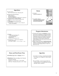

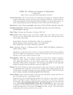
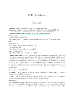


© Copyright 2026