Physical Geology
Laboratory
Streams, water, and surfaces
Exercise emphasizing core objectives
StreaiTI Processes,
Landscapes, Mass Wastage,
and Flood Hazards
CONTRIBUTING AUTHORS
Pamela] .W Gore • Georgia Perimeter College
Richard W Macomber • Long Island University-Brooklyn
Cherukupalli E. Nehru • Brooklyn College (CUNY)
OBJECTIVES AND ACTIVITIES
INTRODUCTION
A. Be able to use topographic maps and stereograms to describe and interpret stream valley
shapes, channel configurations, drainage
patterns, depositional features, and the evolution of meanders.
ACTIVITY 1: Introduction to Stream
Processes and Landscapes
ACTIVITY 2: Meander Evolution on the
Rio Grande
B. Understand erosional and mass wastage
processes that occur at Niagara Falls, and be
able to evaluate rates at which the falls is retreating upstream .
ACTIVITY 3: Mass Wastage at Niagara Falls
C. Be able to construct a flood magnitude/frequency
graph, map floods and flood hazard zones, and
assess the extent of flood hazards along the Flint
River, Georgia.
ACTIVITY 4: Flood Hazard Mapping, Assessment, and Risk
STUDENT MATERIALS
Pencil, eraser, ruler, calculator, 12-inch length of
string.
It all starts with a single raindrop, then another and an-
other. As water drenches the landscape, some soaks into
the ground and becomes groundwater. Some flows
over the ground and into streams and ponds of swface
water. The streams will continue to flow for as long as
they receive a water supply from additional rain,
melting snow, or base flow (groundwater that seeps
into a stream via porous rocks, fractures, and springs).
Perennial streams flow continuously throughout the
year and are represented on topographic maps as blue
lines. Intermittent streams flow only at certain times of
the year, such as rainy seasons or when snow melts in
the spring. They are represented on topographic maps
as blue line segments separated by blue dots (three blue
dots between each line segment). All streams, perennial
and intermittent, have the potential to flood (overflow
their banks). Floods damage more human property in
the United States than any other natural hazard.
Streams are also the single most important
natural agent of land erosion (wearing away of the
land). They erode more sediment from the land than
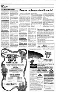
wind, glaciers, or ocean waves. The sediment is transported and eventually deposited, whereupon it is
called alluvium. Alluvium consists of gravel, sand,
silt, and clay deposited in floodplains, point bars,
channel bars, deltas, and alluvial fans (Figure 1).
From Laboratory 11 of Laboratory Manual in Physical Geology, Ninth Edition, American Geological Institute, National Association
of Geoscience Teachers, Richard M. Busch, Dennis Tasa. Copyright © 2011 by Pearson Education, lnc. Published by Pearson
Prentice Hall. All rights reserved.
221
Stream Processes, Landscapes, Mass Wastage, and Flood Ha zards
Main stream
Uplands
~
Heads of
tributaries
A
B. CHANNEL TYPES IN MAP VIEW
Tributaries X, Y
Boundary of
Tributary X drainage
basin (dashed line)
A. STREAM
DRAINAGE
SYSTEM
Yazoo
tributary
Marsh
Point bar building
to right
1
C. FLAT-BOTTOMED VALLEY
WITH MEANDERING
STREAM CHANNEL
Channel bar
D. FLAT-BOTTOMED VALLEY
WITH BRAIDED
CHANNELS AND
SEDIMENT
OVERLOAD
FIGURE 1 General features of stream drainage basins, streams, and stream channels. Arrows indicate current flow in main
stream channels. A. Features of a stream drainage basin . B. Stream channel types as observed in map view. C. Features of<
meandering stream valley. D. Features of a typical braided stream. Braided streams develop in sediment-choked streams.
222
Stream Processes, Landscapes, Mass Wastage, and Flood Hazards
Therefore, stream processes (or fluvial processes)
are among the most important agents that shape
Earth's surface and cause damage to humans and
their property.
PART A: STREAM PROCESSES
AND LANDSCAPES
Recall the last time you experienced a drenching rainstorm. Where did all the water go? During drenching
rainstorms, some of the water seeps slowly into the
ground. But most of the water flows over the ground
before it can seep in. It flows over fields, streets, and
sidewalks as sheets of water several millimeters or
centimeters deep. This is called sheet flow.
Sheet flow moves downslope in response to the
pull of gravity, so the sheets of water flow from streets
and sidewalks to ditches and street gutters. From the
ditches and storm sewers, it flows downhill into small
streams. Small streams merge to form larger streams,
larger streams merge to form rivers, and rivers flow
into lakes and oceans. This entire drainage network,
from the smallest upland tributaries to larger streams,
to the largest river (main stream or main river), is called
a stream drainage system (Figure lA).
Stream Drainage Patterns
Stream drainage systems form characteristic patterns
of drainage, depending on the relief and geology of
the land. The common patterns below are illustrated
in Figure 2:
• Dendritic pattern-resembles the branching of a
tree. Water flow is from the branch-like tributaries
to the trunk-like main stream or river. This pattern
is common where a stream cuts into flat lying layers of rock or sediment. It also develops where a
stream cuts into homogeneous rock (crystalline
igneous rock) or sediment (sand).
• Rectangular pattern-a network of channels
with right-angle bends that form a pattern of
interconnected rectangles and squares. This
pattern often develops over rocks that are
fractured or faulted in two main directions that
are perpendicular (at nearly right angles) and
break the bedrock into rectangular or square
blocks. The streams erode channels along the
perpendicular fractures and faults.
• Radial pattern-channel flow outward from a
central area, resembling the spokes of a wheel.
Water drains from the inside of the pattern, where
the "spokes" nearly meet, to the outside of the
pattern (where the "spokes" are farthest apart) .
223
This pattern develops on conical hills, such as
volcanoes and some structural domes.
• Centripetal pattern-channels converge on a central point, often a lake or playa (dry lake bed), at
the center of a closed basin (a basin from which
surface water cannot drain because there is no
outlet valley).
• Annular pattern-a set of incomplete, concentric
rings of streams connected by short radial channels. This pattern commonly develops on eroding
structural domes and folds that contain alternating folded layers of resistant and nonresistant
rock types.
• Trellis pattern-resembles a vine or climbing rose
bush growing on a trellis, where the main stream
is long and intersected at nearly right angles by
its tributaries. This pattern commonly develops
where alternating layers of resistant and nonresistant rocks have been tilted and eroded to form a
series of parallel ridges and valleys. The main
stream channel cuts through the ridges, and the
main tributaries flow perpendicular to the main
stream and along the valleys (parallel to and
between the ridges).
• Deranged pattern-a random pattern of stream
channels that seem to have no relationship to underlying rock types or geologic structures.
Drainage Basins and Divides
The entire area of land that is drained by one stream, or
an entire stream drainage system, is called a drainage
basin. The linear boundaries that separate one
drainage basin from another are called divides.
Some divides are easy to recognize on maps as
knife-edge ridge crests. However, in regions of lower
relief or rolling hills, the divides separate one gentle
slope from another and are more difficult to locate
precisely (Figure lA, dashed line surrounding the
Tributary X drainage basin). For this reason, divides
cannot always be mapped as distinct lines. In the
absence of detailed elevation data, they must be represented by dashed lines that signify their most probable locations.
You may have heard of something called a
continental divide, which is a narrow strip of land
dividing surface waters that drain in opposite
directions across the continent (Figure 3). The
continental divide in North America is an imaginary
line along the crest of the Rocky Mountains. Rainwater that falls east of the line drains eastward into the
Atlantic Ocean, and rainwater that falls west of the
line drains westward into the Pacific Ocean.
Therefore, North America's continental divide is
sometimes called "The Great Divide."
Stream Processes, Landscapes, Mass Wastage, and Flood Hazards
STREAM DRAINAGE PATTERNS
Dendritic: Irregular pattern of channels that branch like a tree.
Develops on flat lying or homogeneous rock.
Rectangular: Channels have right-angle bends developed along
perpendicular sets of rock fractures or joints.
Radial: Channels radiate outward like spokes of a wheel from a
high point.
Centripetal: Channels converge on the lowest point in a closed
basin from which water cannot drain.
Annular: Long channels form a pattern of concentric circles
connected by short radial channels. Develops on eroded domes
or folds with resistant and nonresistant rock types.
Trellis: A pattern of channels resembling a vine growing on a
trellis. Develops where tilted layers of resistant and nonresistant
rock form parallel ridges and valleys. The main stream channel
cuts through the ridges, and the main tributaries flow along the
valleys parallel to the ridges and at right angles to the main
stream.
Deranged: Channels flow randomly with no relation to underlying
rock types or structures.
FIGURE 2
Some stream drainage patterns and their relationship to bedrock geology.
224
FIGURE 11.3: Lake Scott, Kansas (1976)
0
.5
1 kilometer
hE3E"3E3E31
'I•
3067
'h
41
I
r
I
I
--~ ~~~-~J~ ~
II
II
II
I
I'
II
,;
II
I•
_ _ .,1 ___ ,
1
_ ,
II
: l~ 1
I
II
/
II ] 0 66
•,
)
\
\
_ _L
'
\
_____! ~~
30~24
7. ----~.
I
J01J
1
I (
/
I
/
I
I
I
I
j
I
I
·'
!----
I '
I,
-
r
I
I
/I
f.
{ n
I
!
I
\
"'
I
I.
i!
'I
("i
lsM
rr.
-i·
I
I1 \
I
I
II
I
--~""=
'.}_041
I
.---,---.--"""==-- ·-'~
B
E
,,
R
I
\
I
I
jl
~~~-~3080
I:
I
\
I
).
~2
I
l
J'
I
)j
1-7' --.
14 /
I
"1 -- -- -'8.?6 1
I
I
I
I
j
/
3025
- ~
· - ~ ----~~- -----.
1
\ -·
---
L'
-, ·1,
Stream Processes, Landscapes, Mass Wastage, and Flood Hazards
• Gradient- the steepness of a slope-either the
slope of a valley wall or the slope of a stream
along a selec ted leng th (segment) of its channel
(Figure 4) . Gradient is generally expressed in feet
per mile. This is determined by dividing the vertical rise or fall between two points on the slope (in
feet) by the horizontal distance (run) between
them (in miles). For example, if a stream descends
20 feet over a distance of 40 miles, then its gradient is 20 ft/40 mi, or 0.5 ft/mi. You can estimate
the gradient of a stream by studying the spacing
of contours on a topographic map. Or, you can
precisely calcula te the exact gradient by measuring how much a stream descends along a
measured segment of its course.
Stream Weathering, Transportation,
and Deposition
Three main processes are at work in every stream.
Weathering occurs w here the stream physically erodes
and disintegrates Earth materials and where it chemically decomposes or dissolves Earth materials to form
sediment and aqueo us chem ical solutions. Transportation of these wea thered materials occurs when
they are dragged, bounced, and carried downs tream
(as suspended grains or chemicals in the water).
Deposition occurs if the velocity of the stream drops
(allowing sediments to settle out of the water) or if
parts of the stream evaporate (allowing mineral crystals and oxide residues to form).
The smallest valleys in a drainage basin occur at
its highest elevations, ca lled uplands (Figure 1). In the
uplapds, a stream's (tributary's) point of origin, or
head, may be at a spring or at the start of narrow
runoff channels developed during rainstorms. Erosion
(wearing away rock and sediment) is the dominant
process here, and the stream channels deepen and
erode their V-shaped channels uphill through time-a
process called head ward erosion. Eroded sediment is
transported downstream by the tributaries.
Streams also wea ther and erode their own valleys
along weaknesses in the rocks (fractures, faults), soluble nonresistant layers of rock (salt layers, limestone),
and where there is the least resistance to erosion (see
Figure 2). Rocks composed of h ard, chemically
resistant minerals are generally more resistant to
erosion and form ridges or other hilltops. Rocks composed of soft and more easily weathered minerals are
generally less resistant to erosion and form valleys.
This is commonly called differential erosion of rock.
Headward tributary valleys merge into larger
stream valleys, and these eventually merge into a larger
river valley. Along the way, some new materials are
eroded, and deposits (gravel, sand, mud) may form temporarily, but the main processes at work over the years
in uplands are erosion (head ward erosion and cutting
V-shaped valleys) and transportation of sediment.
The end of a river va lley is the mouth of the river,
where it enters a lake, ocean, or dry basin. At this location, the river wa ter is dispersed into a wider area,
its velocity decreases, and sediment settles out of suspension to form an alluvial deposit (alluvial fan or
delta). If the river water enters a dry basin, then it will
evaporate and precipitate layers of mineral crystals
and oxide residues (in a playa).
River Valley Forms and Processes
The form or shape of a river valley varies with these
main factors:
• Geology-the bedrock geology over which the
stream flows affects the stream's ability to find or
erode its course (Figure 2) .
Gradient
Rise or fall between two points,
measured vertically
.
Distance {run) between the two po1nts,
measured horizontally
= .
Gradient from A to B =
'lr;§::J
100
80
60
ft = 40 ftlmi
1.5mi
¢::
0
<0
g
a;
2
60
.!:
c
0
~
>
Q)
40
[jJ
20
0
0
2
Disti!in
3
ce in .
rn,le~,
u
Gradient from B to C =
4
rl?)i)
40
ft = 13 ft/mi
3.0mi
5
6
FIGURE 4 Gradient is a measure of the steepness of
a slope. As above, gradient is usually determined by dividing the rise or fall (vertical relief) between two points on the
map by the distance (run) between them. It is usually
expressed as a fraction in feet per mile (as above) or meters
per kilometer.
A second way to determine and express the gradient of a
slope is by measuring its steepness in degrees relative to horizontal. Thirdly, gradient can be expressed as a percentage
(also called grade of a slope). For example, a grade of 10%
would mean a grade of 10 units of rise divided by (per) 100
units of distance (i.e., 10 in. per 100 in., 10 m per 100 m).
226
Stream Processes, Landscapes, Mass Wastage, and Flood Hazards
• Base level-the lowest level to which a stream
can theoretically erode. For example, base level is
achieved where a stream enters a lake or ocean.
At that point, the erosional (cutting) power of the
stream is zero and depositional (sediment
accumulation) processes occur.
• Discharge-the rate of stream flow at a given
time and location. Discharge is measured in water
volume per unit of time, commonly cubic feet per
second (ft3 I sec).
• Load-the amount of material (mostly alluvium,
but also plants, trash, and dissolved material) that
is transported by a stream. In the uplands, most
streams have relatively steep gradients, so the
streams cut narrow, V-shaped valleys. Near their
heads, tributaries are quick to transport their load
downstream, where it combines with the loads of
other tributaries. Therefore, the load of the tributaries is transferred to the larger streams and,
eventually, to the main river. The load is eventually
deposited at the mouth of the river, where it
enters a lake, ocean, or dry basin.
From the headwaters to the mouth of a stream, the
gradient decreases, discharge increases, and valleys
generally widen. Along the way, the load of the stream
may exceed the ability of the water to carry it, so the
solid particles accumulate as sedimentary deposits
along the river margins, or banks. Floodplains
develop when alluvium accumulates landward of the
river banks, during floods (Figures lC and lD). However, most flooding events do not submerge the entire
floodplain. The more abundant minor flooding events
deposit sediment only where the water barely
overflows the river's banks. Over time, this creates
natural levees (Figure lC) that are higher than the rest
of the floodplain. If a tributary cannot breach a river's
levee, then it will become a yazoo tributary that flows
parallel to the river (Figure lC).
Still farther downstream, the gradient decreases
even more as discharge and load increase. The stream
valleys develop very wide, flat floodplains with sinuous channels. These channels may become highly sinuous, or meandering (see Figures lB and I C). Erosion
occurs on the outer edge of meanders, which are
called cutbanks. At the same time, point bar deposits
(mostly gravel and sand) accumulate along the inner
edge of meanders. Progressive erosion of cutbanks
and deposition of point bars makes meanders
"migrate" over time.
Channels may cut new paths during floods.
This can cut off the outer edge of a meander, abandoning it to become a crescent-shaped oxbow lake
227
(see Figure I C). When low gradient/high discharge
streams become overloaded with sediment, they may
form braided stream patterns. These consist of braided
channels with linear, underwater sandbars (channel
bars) and islands (see Figures lB and lD).
Some stream valleys have level surfaces that are
higher than the present floodplain. These are remnants
of older floodplains that have been dissected (cut by
younger streams) and are called stream terraces.
Sometimes several levels of stream terraces may be
developed along a stream, resembling steps.
Where a stream enters a lake, ocean, or dry basin,
its velocity decreases dramatically. The stream drops
its sediment load, which accumulates as a triangular
or fan-shaped deposit. In a lake or ocean, such a
deposit is called a delta. A similar fan-shaped deposit
of stream sediment also occurs where a steep-gradient
stream abruptly enters a wide, dry plain, creating an
alluvial fan.
lfiiCQII•M
·'----------~
Introduction to Stream Processes
and Landscapes
Conduct this activity to explore stream processes
and the landscapes they create using topographic
maps (Figures 3, 5, 6, 7).
Meander Evolution on the
Rio Grande
Conduct this activity using Figure 8 to understand
how and why the location of the political boundary between the United States and Mexico is
always changing.
PART B: STREAM EROSION
AND MASS WASTAGE AT
NIAGARA FALLS
Mass wastage is the downslope movement of Earth
materials such as soil, rock, and other debris. It is
common along steep slopes, such as those created
where rivers cut into the land. Some mass wastage
occurs along the steep slopes of the river valleys.
However, mass wastage can also occur in the bed of
the river itself, as it does at Niagara Falls.
------~------------T-----------
1
I
I
I
I
I
I
0
0
16
2
'12
3 kilometers
2 miles
1:62,500
North
\=:l
I~~
"k
21
'---
''~--:
' ! "'
~
,.
1
Stream Processes, Landscapes, Mass Wastage, and Flood Hazards
THE RIO GRANDE
(USA - Mexico Border)
Center of
Rio Grande,
1936
MEANDER TERMS
Oxbow lake
N
~
1992 base map (USGS: Brownsvi lle, TX)
Red 1936 data from USGS map.
Outside
0
1000
2000
3000
4000
5000
\
0
2.0
Miles
~
MATAMOROS,
MEXICO
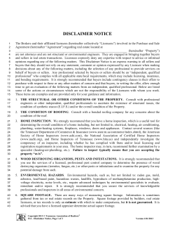
FIGURE 8 Map of the Rio Grande in 1992 (blue) and its former position in 1936 (red) based on U.S. Geological Survey topographic maps (Brownsville, Texas, 1992; West Brownsville, Texas, 1936). The river flows east-southeast. Note the inset box of
meander terms used to describe features of meandering streams.
The Niagara River flows from Lake Erie to Lake
Ontario (Figure 9). The gorge of the Niagara
presents good evidence of the erosion of a caprock
falls, Niagara Falls (Figure 10). The edge (caprock) of
the falls is composed of the resistant Lockport
Dolostone. The retreat of the falls is due to undercutting of mudstones that support the Lockport Dolostone.
Water cascading from the lip of the falls enters the
plunge pool with tremendous force, and the turbulent
water easily erodes the soft mudstones. With the ero-
231
sian of the mudstones, the Lockport Dolostone
collapses.
Mass Wastage at Niagara Falls
Niagara Falls will not exist forever. Conduct
this activity to find out why using Figures 9 and 10.
Stream Processes, Landscapes, Mass Wastage, and Flood Hazards
South to
Lake Erie
North to
Lake Ontario
Queenston
Shale (Brown)
0
Whirlpool
Sandstone
\p
50
.!!!.
~
NIAGARA RIVER
Lockport
Dolostone
l
NIAGARA
GORGE
~----------~
~
g, 100
~
North
t
z
o
dolostone
~ 150 1- - - - - - - - ,
al
:;:
~ 200
.n
Lockport
Dolostone
(Green)
3l
lL
250
sandy
mudstone
NIAGARA
RIVER
h,.,~lli'-'~LlS<,----1
300
FIGURE 10 Cross section of Niagara Falls and geologic
units of the Niagara escarpment.
o~=~==o';2 km
Goat Is.
Niagara
Falls
FIGURE 9 Map of the Niagara Gorge region of Canada
and the United States. The Niagara River flows from Lake
Erie north to Lake Ontario. Niagara Falls is located on the
Niagara River at the head of Niagara Gorge , about half way
between the two lakes.
PART C: FLOOD HAZARD
MAPPING, ASSESSMENT,
AND RISKS
The water level and discharge of a river fluctuates
from day to day, week to week, and month to month.
These changes are measured at gaging stations, with a
permanent water-level indicator and recorder. On a
typical August day in downtown St. Louis, Missouri,
the Mississippi River normally has a discharge of
about 130,000 cubic feet of water per second and water levels well below the boat docks and concre te
levees (retaining walls). However, a t the peak of an
historic 1993 flood, the river discharged more than
a million cubic feet of water per second (8 times the
normal amount), swept away docks, and reached
water levels at the very edge of the highest levees.
When the water level of a river is below the
river 's banks, the river is at a normal stage. When the
water level is even with the banks, the river is at
bankfull stage. And when the water level exceeds
(overflows) the banks, the river is at a flood stage.
The Federal Emergency Management Agency (FEMA:
www.floodsmart.gov) notes that there is a 26% chance
that your home will be flooded over the 30-year
period of a typical home mortgage (compared to a 9%
chance of a home fire).
Early in July 1994, Tropical Storm Alberto entered
Georgia and remained in a fixed position for several
days. More than 20 inches of rain fell in west-central
Georgia over those three days and caused severe
flooding along the Flint River. Montezuma was one of
the towns along the Flint River that was flooded.
Flood Hazard Mapping, Assessment,
and Risk
This part of the laboratory is designed for you to
map and assess the extent of flooding that occurred
at Montezuma, based on river gage records and a
7 ~minu te quadrangle map. You will then use river
gage records to construct a flood magnitude/
frequency graph, determine the probability of
floods of specific magnitudes (flood levels), and revise a map of Montezuma to show the area that can
be expected to be flooded by a 100-year flood.
232
Stream Processes, Landscapes, Mass Wastage, and Flood Hazards
ACTIVITY 1 Introduction to Stream Processes and Landscapes
Name: ___________________________________
Course/Section: __________________________
Materials: Pen cil, ruler, calculator.
A. Trout Run Drainage Basin
1. Complete items a through h.
TOPOGRAPHIC MAP REVIEW FOR DRAINAGE BASIN MAPPING
N
(
~
)
a. This map is contoured in feet.
The contour interval is:
feet.
b. The elevation of point X is:
feet.
c...
c . The elevation of point B is:
feet.
I
::?
0::
§
I
/
I
I
I
lj
x•
e. The distance from A to B is:
mile(s).
I
f.
I
I
I~
)
d . The elevation of point A is:
feet.
•A
I
I
l
•
,g
~I
'1i
I
;/
S' B
The gradient from A to B is:
feet per mile .
g. Lightly shade or color the area
inside each closed contour that
represents a hilltop, then draw
a dashed line to indicate the
drainage divide that surrounds
Trout Run drainage basin .
h. Trout Run flows (drains down
hill) in what direction?
I
I
/
,;
//
(_
/
0
1 mile
2. Imagine that drums of oil were emptied (illegally) at location X above. Is it likely that the oil would wash downhill into
Trout Run? Explain your reasoning.
B. Refer to the topographic map of the Lake Scott quadrangle, Kansas (Figure 3). This area is located within the Great Plains
physiographic province and the Mississippi River Drainage Basin. The Grea t Plains is a relatively flat grassland that
extends from the Rocky Mountains to the Interior Lowlands of North America. It is an. ancient upland surface that tilts
eastward from ru1 elevation of abo ut 5500 fee t along its western bow1dary with the Rocky Mountains to about 2000 feet
above sea level in western Kansas. The upland is the top of a wedge of sedimen t that was weathered ru1d carried eastward
from the Rocky Mountains by a braided stream system that existed from Late Cretaceous to Pliocene time (65- 2.6 Ma).
Modern streams in western Kansas drain eas tward across, and cu t chrum els into, the Great Plains upland surface. Tiny
modern tributaries merge to form larger strean1s that eventually flow into the Mississippi River.
Mi!J§iiiiji!iiii
233
Stream Processes, Landscapes, Mass Wastage, and Flood Hazards
1. What is the gradient of the ancient
upland surface in Figure 3?
Show your work.
2. What is the name of the modern stream drainage pattern from Figure 2 that is developed in the Lake Scott quadrangle,
and what does this drai_nage pattern suggest about the attitude of bedrock layers (the sediment layers beneath the
ancient upland surface) in this area?
3. Notice in Figure 3 that tiny tributaries merge to form larger streams. These larger streams become small rivers that eventually merge to form the Mississippi River. Geoscientists and government agencies classify streams by their order within
this hierarchy of stream sizes from tributaries to rivers. According to this stream order classification, streams with no
tributaries are called first order streams. Second order streams start where two first order streams merge (and may have
additional first order streams as tributaries downstream). Third order streams start where two second order streams
merge (and may have additional first or second order tributaries downstream) . Most geoscientists and goverrunent
agencies include intermittent streams (marked by the blue dot and dash pattern in Figure 3) as part of the stream order
classification. The intermittent stream in Garvin Canyon (Figure 3 and below) has no tributaries so it
is a first order stream. On the enlarged map below draw a dashed line that shows the boundary of the Garvin Canyon
drainage basin.
\
/
~~/
-Jy
·'
'•
/
/
'
("J
a'
4 1
"l.
_i,
I
f ,'
'
/
I
/
(\
(
C)
;:?
._;
"''I
I
I
I
:_
3
- --
~- I
--.
' !
I
.-{
I
··-- ·
/
9
I'
,r
!I
/
y
'i
~
/
I
/
('
/'
lf:/
'•
------
- - - r --·-
- -1
'-
234
Stream Processes, Landscapes, Mass Wastage, and Flood Hazards
4. What is th e gradient of the first
order stream in Garvin Canyon?
(Show your calculations.)
5. What is the stream order of the stream
that occurs in Timber Canyon, and
what is its gradient?
(Show your calculations.)
6. The Mississippi River is a tenth order stream. Based on your answers to the two questions above, state what happens to
the gradient of streams as they increase in order.
7. What do you think happens to the discharge of streams as they increase in order, and what effect do you think this
would have on the relative number of fish living in each stream order within a basin?
C. Examine the landscape of the Waldron, Arkansas, quadrangle (Figure 5). What drainage pattern is developed in this
area, and what does it suggest about the attitude of bedrock layers on this area? Explain your reasoning. (Hint: Refer to
Figure 2. It may also be useful to trace the linear hilltops with a highlighter so you can see their orientation relative to
streams.)
D. Refer to the Voltaire, North Dakota 7.5' quadrangle in Figure 6. Glaciers (composed of a mixture of ice, gravel, sand, and
mud) were present in this region at the end of the Pleistocene Ice Age. When the glaciers melted about 11,000- 12,000 years
ago, a thick layer of sand and gravel was deposited on top of the bedrock, and streams began forming from the glacial
meltwater. Therefore, streams have been eroding and shaping this landscape for about 11,000-12,000 years.
1. What is the width of the modern floodplain of
the Souris River measured along line X-X'?
2. What was the maximum width of the Souris River floodplain in the past (measured along line X-X') and how can you tell?
3. Give one reason why the Souris River floodplain was wider in the past.
4. Notice the marsh in sec. 9 (Figure 6) and the depression on which it is located . What was this depression before it
became a marsh?
...,...,i!i,ii
235
Stream Processes, Landscapes, Mass Wastage, and Flood Hazards
E. Refer to the Ennis Montana 15' quadrangle in Figure 7. Some rivers are subject to large floods, either seasonal or periodic.
In mountains, trus flooding is due to snow melt. In deserts, it is caused by thunderstorms. During such times, rivers transport exceptionally large volumes of sediment. This ca uses characteristic features, two of which are braided channels and alluvial fans. Both features are relatively common in arid mountainous regions, such as the Ermis, Montana, area in Figure 7.
(Both features also can occur wherever conditions are right, even at construction sites!)
1. What was the source of the sediments that have accwnulated on the Cedar Creek Alluvial Fan?
2. Notice the stream between sections 22 and 15 northeast of Lawton Ranch that discharges onto the Cedar Creek
Alluvial Fan.
a. What is the stream order classification of that stream just before it enters the alluvial fan?
b. What happens to that stream's gradient and order as it enters the alluvial fan, and how does this contrib ute to the formation of the alluvial fan?
3. What main stream channel types (shown in Figure lB) are present on:
a. the streams in the forested south eastern corner of this map?
b. the Cedar Creek Alluvial Fan?
c. the valley of the Madison River (northwestern portion of Figure 7)?
236
Stream Processes, Landscapes, Mass Wastage, and Flood Hazards
ACTIVITY 2 Meander Evolution on the Rio Grande
Name: ___________________________________
Course/Section: ---------------------------
Materials: Pencil, ruler, calculator.
Refer to Figure 8 showing the meandering Rio Grande, the river that forms the national border between Mexico and the
United States. Notice that the position of the river changed in many places between 1936 (red line and leaders by lettered
features) and 1992 (blue water bodies and leaders by lettered features). Study the meander terms provided in Figure 8,
and then proceed to the questions below.
A. Study the meander cutbanks labeled A through G. The red .leader from each letter points to the cutbank's location in 1936.
The blue leader from each letter points to the cutbank's location in 1992. In what two general directions (relative to the
meander, relative to the direction of river flow) have these cutbanks moved?
B. Study locations Hand I.
1. In what country were Hand I located in 1936?
2. In what country were Hand I located in 1992?
3. Explain a process that probably caused .locations Hand I to change from meanders to oxbow lakes.
C. Based on your answer .i n item B3, predict how the river will change in the future at locations Jand K.
D. What are features L, M, and N, and what do they indicate about the historical path of the Rio Grande?
E. What is the average rate at which meanders like A through G migrated here (in meters per year) from 1936 to 1992?
Explain your reasoning and calculations.
F. Explain in steps how a meander evolves from the earliest stage of its history as a broad slightly sinuous meander to the
stage when an oxbow lake forms.
237
Stream Processes, Landscapes, Mass Wastage, an.d Flood Hazards
ACTIVITY 3 Mass Wastage at Niagara Falls
Name: _____________________________________
Course/Section: _ _ _ _ _ _ _ _ _ _ _ _ __
Materials: Pencil, eraser, ruler, calculator, 12-inch length of string.
A. Geologic evidence indicates that the Niagara River began to cut its gorge (Niagara Gorge) about 11,000 years ago as the
Laurentide Ice Sheet retreated from the area. The ice started at the Niagara Escarpment shown in Figure 9 and receded
(melted back) north to form the basin of Lake Ontario. The Niagara Gorge started at th e Niagara Escarpment and retreated
south to its present location. Based on this geochronology and the length of Niagara Gorge, calculate the average rate of
falls retreat in ern I year. Show your calculations.
B. Name as many factors as you can that could ca use the falls to retreat a t a faster rate.
C. Name as many factors as you can that co uld cause the falls to retreat more slowly.
D. Niagara Falls is about 35 km north of Lake Erie, and it is retreating so uthward . If the falls was to continue its retreat at the
average rate calculated in A, then how many years from now would the falls reach Lake Erie?
238
Stream Processes, Landscapes, Mass Wastage, and Flood Hazards
ACTIVITY 4 Flood Hazard Mapping, Assessment, and Risk
Name: _____________________________________
Course/Section: _______________
Materials: Pencil, calculator, ruler.
A. On the Montezuma, Georgia topographic map, locate the gaging station along the east side of the Flint River near the
center of the map, between Montezuma and Oglethorpe. This U.S. Geological Survey (USGS) gaging station is located at
an elevation of 255.83 feet above sea level, and the river is considered to be at flood stage when it is 20 feet above this level
(275.83 feet) . The old flood record was 27.40 feet above the gaging station (1929), but the July 1994 flood established a new
record at 35.11 feet above the gaging station, or 289.94 feet above sea level. This corresponds almost exactly to the 290-foot
contour line on the map. Trace the 290-foot contour line on both sides of the Flint River on the map. Label the area within
these contours (land areas lower than 290 feet) as the 1994 Flood Hazard Zone.
B. Assess the damage caused by the July 1994 flood (using the topographic map).
1. Notice that the gaging station is located adjacent to highway 26-49-90. Was it possible to travel from Montezuma to
Oglethorpe on this highway during the 1994 flood? Explain.
2. Notice the railroad tracks parallel to (and south of) highway 26-49-90 between Montezuma and Oglethorpe. Was it
possible to travel on these railroads during the 1994 flood? Explain.
C. Notice line X-Y near the top center part of the topographic map.
1. The map shows the Flint River at its normal stage. What is the width
(in km) of the Flint River at its normal stage
along line X-Y?
2. What was the width of the river (in km) along this line when it was at
maximum flood stage (290 feet) during the July 1994 flood?
D. Notice the floodplain of the Flint .River along line X-Y. It is the relatively flat (as indicated by widely spaced contour lines)
marshy land between the river and the steep (as indicated by more closely spaced contour lines) walls of the valley that are
created by erosion during floods.
1. What is the elevation (in feet above sea level) of the floodplain on the west side of the river along line X-Y?
2. How deep (in feet above sea level) was the water that covered
that floodplain during the 1994 flood? (Explain your
reasoning or show your mathematical calculation.)
3. Did the 1994 flood (i.e., the highest river level ever recorded here) stay within the floodplain and its bounding valley
slopes? Does this suggest that the 1994 flood was of normal or abnormal magnitude (severity) for this river? Explain
your reasoning.
E. The USGS recorded annual high stages (elevation of water level) of the Flint River at the Montezuma gaging station for 99
years (1897 and 1905- 2002). Pa1·ts of the data have been sununarized in the Flood Data Table.
1. The annual highest stages of the Flint River (S) were ranked in severity from S = 1 (highest aru1ual high stage ever
recorded; i.e., the 1994 flood) to S = 99 (lowest annual high stage). Data for 14 of these ranked yea1·s are provided in the
Flood Data Table and can be used to calculate recurrence interval for each magnitude (rank, S). Recurrence interval (or
Miil§iii§i!iii
239
Stream Processes, Landscapes, Mass Wastage, and Flood Hazards
return period) is the average number of years between occurrences of a flood of a given rank (S) or greater than that
given rank. Recurrence interval for a rank of flood can be calculated as: Rl = (n + 1)/S. Calculate the recurrence interval
for ranks 1- 5 and write them in the table. This has already been done for ranks of 20, 30, 40, 50, 60, 70, 80, 90, and 99.
2. Notice that a recurrence interval of 5.0 means that there is a 1-in-5 probability (or 20% chance) that an event of that
magnitude will occur in any given year. This is known as a 5-year flood. What is a 100-year flood ?
3. Plot (as exactly as you can) points on the flood magnitude/ frequency graph (below the Flood Data Table) for all
14 ranks of cumual high river stage in the Flood Data Table. Then use a ruler to draw a line through the points (cu1d on to
the right edge of the graph) so the nwnber of, or distance to, points above cu1d below the line is similar.
4. Your completed flood magnitude/frequency graph ccu1 now be used to estimate the probability of future floods of a
given magnitude and frequency. A 10-year flood on the Flint River is the point where the line in your graph crosses the
flood frequency (RI, return period) of 10 years. What is the probability that a future 10-year flood will occur in any given
year, and what will be its magnitude (river elevation in feet above sea level)?
5. What is the probability for cu1y given year that a flood on the Flint River at Montezuma, GA will reach cu1 elevation of
275 feet above sea level?
F. Most homeowners insurance policies do not insure against floods, even though floods cause more dcunage than any other
natural hazard. Homeowners must obtain private or federal flood insurance in addition to their base homeowners policy.
The National Flood Insurcu1ee Progrcun (NFIP), a Division of the Federal Emergency Management Agency (FEMA), helps
corrunw1ities develop corrective and preventative measures for reducing future flood dcunage. The progrcun centers on
floodplain identification, mapping, and management. In return, members of these communities are eligible for discounts
on federal flood insurance. The rates are determined on the basis of a community's FIRM (Flood Insurance Rate Map), an
official map of the community on which FEMA has delineated flood hazard areas cu1d risk premium zones (with discount
rates). The hazard areas on a FIRM are defined on a base flood elevation (BFE)-the computed elevation to which flood water
is estimated to rise during a base flood. The regulatory-standcu·d base flood elevation is the 100-year flood elevation. Based
on your graph, what is the BFE for Montezuma, GA?
G. The 1996 FEMA FIRM for Montezuma, GA shows hazard areas designated zone A. Zone A is the official designation for
areas expected to be inundated by 100-year flooding even though no BFEs have been determined. The location of zone A
(shaded gray) is shown on the Flood Hazard Map of a portion of the Montezuma, GA 71/2 minute map. Your work above
can be used to revise the flood hazard area. Place a dark line on this map (as exactly as you ccu1) to show the elevation
contour of the BFE for this corrunw1ity (your cu1swer in item F). Your revised map reflects more accurately what area will
be inundated by a 100-year flood. In general, how is the BFE line that you have plotted different from the bOLmdary of zone
A plotted by FEMA on its 1996 FIRM?
H. Note that the elevation of the 100-year flood is estimated based on historical (existing) data. As in the excunple of
Montezuma, GA, a new flood that sets a new flood record will chcu1ge the flood magnitude/frequency graph cu1d the estimated BFE. You should always obtain the latest flood hazard map / graph to estimate flood probability for a given location.
Determine the flood risk where you live (or another address of your choice) at http:/ /www.floodsmart.gov /floodsmart/
(One Step Flood Risk Profile).
240
t~)
ACTIVITY 4: Montezuma, Georgia (1985) Topographic Map
o
.5
HE3E3E3
o
v.
1 kilometer
E3
'/2
1
1 .
North
1 mile
Georgia
Quadrangle location
...
N
..a.
....
Stream Processes, Landscapes, Mass Wastage, and Flood Hazards
Flood Data Table
Recurrence Intervals for Selected, Ranked, Annual Highest Stages of the Flint River over 99 Years of
Observation (1897 and 1905-2002) at Montezuma, Georgia (USGS Station 02349500, data from USGS)
Year
(*n = 99)
Rive r elevation
above gage,
in feet
Gage elevation
above sea
level, in feet
River elevation
above sea
level, in feet
1 (highest)
1994
34.1 1
255 .83
289.9
1 in 100
2
1929
27.40
255.83
283.2
1 in 50
3
1990
26.05
255 .83
281 .9
1 in 33.3
3%
4
1897
26.00
255.83
281.8
1 in 25
4%
5
20
1949
25 .20
255 .83
281.0
1 in 20
5%
1928
21.30
255 .83
277. 1
5.0
1 in 5
20%
29%
43%
Ran k of annual
high est ri ver
stage (S)
Recurrence
interval**
(RI), in years
Probability of
Percent chance
occ urring in
of occ urring in
any given year any given year***
1%
2%
30
1912
20.60
255 .83
276.4
3.4
1 in 3.4
40
1959
19.30
255.83
275.1
2.3
1 in 2.3
50
1960
18.50
255.83
274.3
2.0
60
70
1934
17.70
255 .83
273.5
1.8
1 in 2
1 in 1. 8
17.25
255.83
273. 1
1.5
1 in 1.5
80
1974
1967
56 %
67 %
14.76
255 .83
270.6
1.3
1 in 1.3
77 %
90
1907
13.00
255.83
268.8
1.1
1 in 1.1
91 %
99 (lowest)
2002
8.99
255.83
264.7
1.0
1 in 1
100 %
50%
"n = number of years of annual observations = 99
--·Recurrence Interval (AI)= (n + 1) IS= average number of years between occu rrences of an event of this magnitude or greater.
....... Percent chance of occurrence= 1 I AI x 100.
320
10-year flood
100-year flood
1000-year flood
~
~
~
(jj
>
.3
310
"'
<1>
(/)
<1>
>
0
.D
"'
300
Q5
<1>
LL
.S
c
0
-~
290
>
<1>
w
ID>
a:
iJj
"0
280
-~
c
Ol
"'
::;,
"0
0
0
270
u:::
260
1
2
3
4
5 6 7 8 9 10
20
30
40 50
100
Flood Frequency : Rec urrence Interval (RI)
242
200
400
1000
Stream Processes, Landscapes, Mas s Wastage, and Flood Hazards
Flood Hazard Map
Portion of Montezuma, Georgia U.S.G.S. 7 1/2 Minute Topographic Quad range Map
Shaded Gray to Show FEMA FIRM Zone A (area inundated by 100-year flooding) as
Adapted From FEMA FIRM# 13193C0275D (1996)
••
•
I
Scale 1:12,000
Contour Interval = 10 feet
-
0
.
. ..
. .
I
~ ·.
1 km
= Bou ndary of FIRM Zo ne A (FEMA FIRM #1 3193C0275 D; Effective 1996) (area inundated by 100-year fl oodi ng is shaded gray)
243
I
I