1. science
2. mathematics
3. geometry

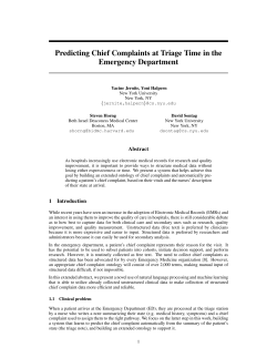
IEEE TRANSACTIONS ON PATTERN ANALYSIS AND MACHINE INTELLIGENCE, VOL. ?, NO. ?, ? ?
1
Effective Unconstrained Face Recognition by
Combining Multiple Descriptors and Learned
Background Statistics
Lior Wolf, Member, IEEE, Tal Hassner, and Yaniv Taigman
Abstract—Computer Vision and Biometrics systems have demonstrated considerable improvement in recognizing and verifying faces
in digital images. Still, recognizing faces appearing in unconstrained, natural conditions remains a challenging task. In this paper we
present a face-image, pair-matching approach primarily developed and tested on the “Labeled Faces in the Wild” (LFW) benchmark that
reflect the challenges of face recognition from unconstrained images. The approach we propose makes the following contributions. (a)
We present a family of novel face-image descriptors designed to capture statistics of local patch similarities. (b) We demonstrate
how semi-labeled background samples may be used to better evaluate image similarities. To this end we describe a number of
novel, effective similarity measures. (c) We show how labeled background samples, when available, may further improve classification
performance, by employing a unique pair-matching pipeline. We present state-of-the-art results on the LFW pair-matching benchmarks.
In addition, we show our system to be well suited for multi-label face classification (recognition) problems. We perform recognition tests
on LFW images as well images from the laboratory controlled multiPIE database.
Index Terms—I.5.4.d Face and gesture recognition, I.5.3.b Similarity measures, Face recognition, Image descriptors, Similarity
measures.
F
1
I NTRODUCTION
R
RECENT years have seen an explosion of visual
media available through the Internet. This mounting volume of images and videos brings with it new
opportunities and new challenges for Computer Vision
applications. Face recognition applications in particular are now, more than ever, required to handle large
quantities of images and remain accurate even when
presented with images taken under unconstrained conditions. Facebook and Picasa web photo albums, for example, typically contain thousands of face images, most of
which were obtained without control over facial expression, viewing angle, lighting conditions, occlusions and
image quality. Such image collections strongly motivate
research into recognition of faces in unconstrained images and at the same time provide an abundance of data
for testing and developing new recognition techniques.
New recognition benchmarks have recently been published to facilitate the development of methods for face
recognition under such challenging conditions. These
include the “Labeled Faces in the Wild” (LFW) image set
and benchmark [5], and the “Public Figures” (PubFig)
data set of [6]. Both data sets consist of face images
• Parts of this manuscript have been published in [1]–[4].
• L. Wolf is with the School of Computer Science, Tel-Aviv University, Israel.
E-mail: [email protected]
• T. Hassner is with the Computer Science Division, The Open University
of Israel.
E-mail: [email protected]
• Y. Taigman is with face.com and with the School of Computer Science,
Tel-Aviv University, Israel.
E-mail: [email protected]
automatically harvested from news websites of known
(labeled) people. The images in these sets thus attempt
to capture the variability typical to unconstrained, “in
the wild”, face recognition problems. The LFW dataset in
particular is published with a specific benchmark, which
focuses on the face recognition task of pair matching (also
referred to as “face verification”). In this task, given
two face images, the goal is to decide whether the two
pictures are of the same individual. Since its publication,
the LFW benchmark has attracted quite a lot of attention,
with various research teams contributing state-of-the-art
pair-matching results [7].
This paper describes face pair-matching and classification methods developed and tested on the LFW benchmark and motivated by the following two principles.
The first is that multiple image descriptors may be combined, each one complementing the others and together
providing improved classification results. To this end
we describe a family of novel descriptors which we
show to be particularly useful for face recognition. The
second principle is that face recognition performance
(and indeed, classification performance in general) may
greatly benefit from the availability of labeled background
information. Here we refer to background samples as
labeled training samples that do not belong to the classes
being learned.
Our contributions in this paper are therefore the following:
1) We develop a family of novel image descriptors that are able to improve classification performance of multi-option recognition as well as
pair-matching of face images. These descriptors
IEEE TRANSACTIONS ON PATTERN ANALYSIS AND MACHINE INTELLIGENCE, VOL. ?, NO. ?, ? ?
compute an image representation from local patch
statistics. Here, we show these descriptors to provide information which is complementary to existing feature methods (see section 3).
2) We present two novel similarity measures, the OneShot and the Two-Shot Similarity measures, both
based on discriminative learning and both employing semi-labeled, background samples (section 4).
3) Finally, we show how labeled background samples
may also be exploited to obtain more accurate
classification results (section 4.4).
2
E XISTING
METHODS
This paper touches on a number of well established
research fields. We briefly survey relevant existing work.
Face recognition Face recognition is one of the most
well-studied problems in Computer Vision and Biometrics and the literature on this problem is vast. Over
the years a number of successful face-image data-sets
have been published in an effort to facilitate research on
face recognition. These include the Facial Recognition
Technology (FERET) Database [8], the Face Recognition Grand Challenge (FRGC) facial images and depths
along with accompanying benchmark tests [9], [10] and
its successor, the Face Recognition Vendor Test (FRVT)
database and benchmark [11], the CMU Pose Illumination and Expression (CMU-PIE) database [12] and its
extension, the multi-PIE database [13].
These image sets were all designed to capture different
sources of variability likely to be encountered by face
recognition systems. These include illumination, pose,
expression and more. However, they were all produced
in controlled, laboratory settings. To provide researchers
with a wider and more arbitrary range of viewing conditions, the Labeled Faces in the Wild (LFW) [5] and its extension, the Public Figure (PubFig) [6] sets were devised.
These image sets include images automatically collected
from Internet web pages; images were added to these
sets if they include a face detected by a Viola and Jones
face detector [14]. The facial images included in the LFW
data set therefore demonstrate quite a bit of variability.
Since its recent publication, a lot of attention has been
focused on improving performance on the benchmarks
associated with the LFW database (see, e.g., [1]–[3], [6],
[15]–[19]).
Descriptor based methods for face recognition Face
Images can be most readily described by statistics derived from their intensities. Intensities have thus served
in many template-based methods. The intensities were
sometimes normalized and sometimes replaced by edge
responses [20]. More recently [21]–[23], Gabor wavelets
have been used to describe the image appearance.
A texture descriptor called Local Binary Patterns
(LBP) [24]–[26] has been shown to be extremely effective
for face recognition [27]. The most simple form of LBP
is created at a particular pixel location by threshholding
the 3 × 3 neighborhood surrounding the pixel with the
2
central pixel’s intensity value, and treating the subsequent pattern of 8 bits as a binary number (Fig. 1).
A histogram of these binary numbers in a predefined
region is then used to encode the appearance of that
region. The LBP representation of a given face image is
generated by dividing the image into a grid of windows
and computing histograms of the LBP values within
each window. The concatenation of all these histograms
constitutes the image’s signature.
In this work we propose a patch-based descriptor that
has some similarities to a variant of LBP called CenterSymmetric LBP (CSLBP) [28]. In CSLBP, eight intensities
around a central point are measured. These intensities
are spread evenly at a circle every 45 degrees starting
at 12 o’clock. The binary vector encoding the local appearence at the central point, consists of four bits which
contain the comparison of intensities to intensities on the
symmetric position (180 degrees/ 6 hours difference).
Multi-block LBP [29] is an LBP variant that replaces intensity values in the computation of LBP with the mean
intensity value of image blocks. Despite the similarity
in terms, this method is very much different from our
own. Multi-block LBP is shown to be effective for face
detection, and in our initial set of experiments does not
perform well for face recognition.
Modern image similarity learning techniques The
literature on similarity functions is extensive. Some similarity measures proposed in the past have been hand
crafted (e.g., [30], [31]). Alternatively, a growing number
of authors have proposed tailoring similarity measures
to available training data by applying learning techniques (e.g., [32]–[36]). In all these methods testing is
performed using models (or similarity measures) learned
beforehand.
The One-Shot and Two-Shot Similarity scores (OSS
and TSS scores) introduced here (Section 4.1) are alternative approaches, designed to utilize “background”
samples. OSS and TSS both draw their motivation from
the growing number of so called “One-Shot Learning”
techniques; that is, methods which learn from one or
few training examples (see for example [37], [38]). Unlike previous methods for computing similarities, these
novel similarity measures are computed by training a
discriminative model exclusive to the two signals being
compared, by using a set of background samples. As we
will show, both measures are instrumental in obtaining
state-of-the-art results on the Labeled Faces in the Wild
(LFW) image pair-matching and provided boosted performance in multi-subject recognition problems.
Employing background samples differs from semisupervised learning [39] and from transductive learning [40] since in both cases the unlabeled samples belong
to the set of training classes. It differs from flavors of
transfer learning that use unlabeled samples [41], since
they use separate supervised learning tasks in order to
benefit from the unlabeled set.
Although learning with background samples can be
seen as belonging to the group of techniques called
IEEE TRANSACTIONS ON PATTERN ANALYSIS AND MACHINE INTELLIGENCE, VOL. ?, NO. ?, ? ?
5
6
2
2
4
3
1
1
4
3
Threshold
1
1
0
0
0
0
0
1
Encode
01100100
(a)
(b)
(c)
Fig. 1. (a) The LBP image-texture descriptor is computed locally at each pixel location. It considers a small
neighborhood of a pixel, and thresholds all values by the central pixel’s value. The bits which represent the comparison
results are then transformed into a binary number. The histogram of these numbers is used as a signature describing
the texture of the image. (b-c) Present an example image from the LFW data set, and its LBP encoding (different
intensities representing different codes.)
“learning with side-information”, it differs from existing
methods in the literature known to us. In particular,
some of the previous contributions, e.g., [36], [42], [43],
require having training samples with the same identity.
Other side-information contributions, e.g., [44] assume
that the variability in the side information differs from
that in the relevant data.
Also related to our work is the recent method of [6].
They study trait- or identity-based classifier-outputs as a
feature for identification. Unlike our work, their method
encodes one vector per face image whereas we encode
pairs of images.
As a part of our supervised (“unrestricted”) pipeline,
we use a particular metric learning method called Information Theoretic Metric Learning (ITML) [45], [46].
ITML is a supervised metric learning technique for learning a Mahalanobis distance. It uses pairs of examples
belonging to the same class (in our case, images of the
same person) which are constrained to have similarities
below a specified threshold. The similarities of pairs
of points from different classes are constrained to have
similarities above a second threshold. A regularization
term ensures that the learned metric is similar to the
original metric. The ITML method was shown to be
extremely potent in Computer Vision problems [46]. The
OSS and the TSS methods are both semi-supervised
learning techniques. We show the OSS to work particularly well when combined with the supervised ITML
method.
Patch-based approaches in recognition In this work
we build upon methods which utilize image-patches,
sometimes referred to as windows or blocks, for recognition. The patch based approach of [47] provides state
of the art capabilities in similarity learning of faces and
of general images. Other successful object recognition
systems based on patches include the hierarchical system
of [48].
The ability to detect local texture properties by examining the cross correlation between a central patch and
nearby patches has been demonstrated in the texture
segmentation system of [49]. In [50] a central patch was
compared to surrounding patches to create a descriptor
which extends the shape-context [30] descriptor to intensity images. The resulting descriptor has been shown to
be highly invariant to image style and local appearance.
3
N OVEL
PATCH BASED
LBP S
The LBP descriptor and its variants (e.g., [29], [51]) use
short binary strings to encode properties of the local
micro-texture around each pixel. CSLBP [28], for example, encodes in each pixel the gradient signs at the pixel
in four different angles. Here we propose two families of
related descriptors, the Three-Patch LBP and the FourPatch LBP descriptors1 , designed to encode additional
types of local texture information.
The design of these descriptors is inspired by the
Self-Similarity descriptor of [50]. Specifically, we explore
ways of using short bit strings to encode similarities
between neighboring patches of pixels in an effort to
capture information complementary to that of pixelbased descriptors. Thus, employing patch based and
pixel based descriptors in concert improves the overall accuracy of a classification system. In fact, a recent
independent study [19] has shown that using our FPLBP
descriptors described below to encode face images was
only slightly worst than using collections of SIFT [52]
descriptors, while being an order of magnitude more
compact.
3.1
Three-Patch LBP Codes
Three-Patch LBP (TPLBP) codes are produced by comparing the values of three patches to produce a single bit
value in the code assigned to each pixel. For each pixel
in the image, we consider a w × w patch centered on the
pixel, and S additional patches distributed uniformly in
a ring of radius r around it (Fig. 2). For a parameter
1. MATLAB code for computing both descriptors is available online
at http://www.openu.ac.il/home/hassner/projects/Patchlbp/
IEEE TRANSACTIONS ON PATTERN ANALYSIS AND MACHINE INTELLIGENCE, VOL. ?, NO. ?, ? ?
α, we take pairs of patches, α-patches apart along the
circle, and compare their values with those of the central
patch. The value of a single bit is set according to which
of the two patches is more similar to the central patch.
The resulting code has S bits per pixel. Specifically, we
produce the Three-Patch LBP by applying the following
formula to each pixel:
TPLBPr,S,w,α (p) =
S
X
f (d(Ci , Cp )−d(Ci+α
i
mod S , Cp ))2
i=1
(1)
Where Ci and Ci+α mod S are two patches along the ring
and Cp is the central patch. The function d(·, ·) is any
distance function between two patches (e.g., L2 norm of
their gray level differences) and f is defined as:
1 if x ≥ τ
f (x) =
(2)
0 if x < τ
We use a value τ slightly larger than zero (e.g., τ = 0.01)
to provide some stability in uniform regions, similarly
to [28]. In practice, we use nearest neighbor sampling to
obtain the patches instead of interpolating their values,
as this speeds up processing with little or no effect on
performance.
Once encoded, an image’s signature is produced similarly to that of the CSLBP descriptor [28]. The image is
divided into a grid of none-overlapping regions and a
histogram measuring the frequency of each binary code
is computed for each region. Each of these histograms
are normalized to unit length, their values truncated at
0.2, and then once again normalized to unit length. An
image is represented by these histograms concatenated
to a single vector.
3.2
Four-Patch LBP Codes
For every pixel in the image, we look at two rings of
radii r1 and r2 centered on the pixel, and S patches of
size w × w spread out evenly on each ring (Fig. 3). To
produce the Four-Patch LBP (FPLBP) codes we compare
two center symmetric patches in the inner ring with two
center symmetric patches in the outer ring positioned
α patches away along the circle (say, clockwise). One
bit in each pixel’s code is set according to which of the
two pairs being compared is more similar. Thus, for S
patches along each circle we have S/2 center symmetric
pairs which is the length of the binary codes produced.
The resulting codes, similarly to the CS-LBP descriptors,
are extremely compact, typically requiring histograms of
only 16 values, yet have very high descriptive power, as
was shown in [19].
The formal definition of the FPLBP code is as follows:
FPLBPr1 ,r2 ,S,w,α (p) =
S/2
X
f (d(C1i , C2,i+α
mod S )−
i=1
d(C1,i+S/2 , C2,i+S/2+α
i
mod S ))2
(3)
4
The final image signature is produced by using the
same two-step normalization procedure described in
Section 3.1.
4
C OMPUTING
SIMILARITY
WITH
BACK -
GROUND SAMPLES
In a learning framework, we define background samples as
samples that do not belong to the classes being learned.
Collecting such samples is often easy as they do not
require labeling. In a face identification scenario these
samples could be a face set of individuals not among
those which the system is being trained to recognize.
Besides being easy to collect, we believe such examples
may provide valuable information about which images
may be considered “the same” and which may not. In
this section we present three novel similarity measures
designed to exploit available background information for
more accurate signal classification.
Why would background samples be useful for defining similarity functions? The sample vectors are embedded in a vector space in which various metrics can be
employed. In order to know which metric is most suitable for the similarity task at hand, the underlying structure of the manifold on which the samples reside needs
to be analyzed. Supervised learning can sometimes be
used, but may require extra labeling information. On
the other hand, background samples without additional
information directly answer questions such as “is this
sample closer to that one than to a typical example
from the background set?” (the One-Shot Similarity, Section 4.1); “are these two examples well separated from
the background sample set?” (the Two-shot Similarity,
Section 4.1); and “do these two samples have similar sets
of neighboring samples in the background set?” (ranking
based similarity, Section 4.3).
4.1
The One-Shot and Two-Shot Similarity Measures
Given two vectors I and J their One-Shot Similarity
(OSS) score is computed by considering a training set of
background sample vectors A. This set contains examples of items not belonging to the same class as neither
I nor J, but are otherwise unlabeled. A measure of the
similarity of I and J is then obtained as follows (see also
Fig. 4 (a)). First, a discriminative model is learned with I
as a single positive example, and A as a set of negative
examples. This model is then used to classify the vector,
J, and obtain a confidence score. The nature of this score
depends on the classifier used. Using linear SVM, for
example, this score may be the signed distance of J from
the hyperplane separating I and A. A second such score
is then obtained by repeating the same process with the
roles of I and J switched. The final OSS score is the
average of these two scores.
The Two-Shot similarity (TSS) score is obtained in a
single step by modifying the process described above
(see also Fig. 4 (b)). Again, we consider the same auxiliary set of negative examples A. This time, however,
IEEE TRANSACTIONS ON PATTERN ANALYSIS AND MACHINE INTELLIGENCE, VOL. ?, NO. ?, ? ?
w
C2
C1
C3
α
TPLBPr,8,3,2 (p) =
f (d(C0 , Cp ) − d(C2 , Cp ))20 +
f (d(C1 , Cp ) − d(C3 , Cp ))21 +
f (d(C2 , Cp ) − d(C4 , Cp ))22 +
f (d(C3 , Cp ) − d(C5 , Cp ))23 +
f (d(C4 , Cp ) − d(C6 , Cp ))24 +
f (d(C5 , Cp ) − d(C7 , Cp ))25 +
f (d(C6 , Cp ) − d(C0 , Cp ))26 +
f (d(C7 , Cp ) − d(C1 , Cp ))27
(b)
w
r
CP
C0
C4
C5
C7
5
C6
(a)
(c)
Fig. 2. (a) The Three-Patch LBP code with α = 2 and S = 8. (b) The TPLBP code computed with parameters S = 8,
w = 3, and α = 2. (c) Code image produced from the image in Fig. 1(b).
c22
r2
C21
α
c23
c12
c11
c20
c13
r1
C10
c17
FPLBPr1,r2,8,3,1 (p) =
f (d(C10 , C21 ) − d(C14 , C25 ))20 +
f (d(C11 , C22 ) − d(C15 , C26 ))21 +
f (d(C12 , C23 ) − d(C16 , C27 ))22 +
f (d(C13 , C24 ) − d(C17 , C28 ))23
c24
C14
c15
c16
c27
α
C25
c26
(a)
(b)
(c)
Fig. 3. (a) The Four-Patch LBP code. Four patches involved in computing a single bit value with parameter α = 1 are
highlighted. (b) The FPLBP code computed with parameters S = 8, w = 3, and α = 1. (c) Code image produced from
the image in Fig. 1(b).
not (I  J)
not J
not I
J
I
J
I
(a)
(b)
Fig. 4. OSS and TSS scores illustrated. (a) The OSS
score is obtained by computing two discriminative models. (b) The Two-Shot score is computed from a single
model, taking I and J as a positive set, and A as a
negative set. The Two-Shot score reflects the quality of
this model.
we train a single discriminative model using both I
and J as positive examples, and the set A as a set of
negative examples. The Two-Shot score is then defined
as a measure of how well this model discriminates the
two sets. Again, the particular definition of this score depends on the underlying classifier used. Using the SVM
classifier, for example, this can simply be the width of the
margin between the two sets. In the following sections
we provide detailed analysis of this new similarity score.
4.2 Computing the One-Shot and Two-Shot Similarities
The OSS and TSS scores are actually meta-similarities
which can be fitted to work with almost any discriminative learning algorithm. In our experiments, we focused
on the Fisher Discriminant Analysis (FDA or LDA) [53],
[54] as the underlying classifier. Similarities based on
LDA can be efficiently computed by exploiting the fact
that the set A of negative samples is used repeatedly,
and that the positive class, which contains just one or
two elements, contributes either nothing or a rank-one
matrix to the within class covariance matrix.
We focus on binary LDA, which is relevant to this
work. Let pi ∈ Rd , i = 1, 2, ..., m1 be a set of positive
training examples, and let ni ∈ Rd , i = 1, 2, ..., m2 be a
set of negative training examples. Let µ be the average
of all points and µp (resp. µn ) be the average of the
positive (negative) training set. Two matrices are then
considered [55], SB measuring the covariance of the class
centers, and SW , which is the sum of the covariance
matrices of each class. The LDA algorithm computes a
projection v which maximizes the quotient:
v = arg max
v
v > SB v
v > SW v
(4)
IEEE TRANSACTIONS ON PATTERN ANALYSIS AND MACHINE INTELLIGENCE, VOL. ?, NO. ?, ? ?
In the two class case, v is easily determined as:
v=
+
SW
(µp − µn )
+
kSW (µp − µn )k
(5)
+
Note that we use the pseudo-inverse SW
instead of
−1
the inverse SW in order to deal with cases where the
within-class covariance matrix is not full rank. This is
equivalent to requiring in Eq. 4 that v be spanned by
the training vectors.
Once v has been computed, the classification of a new
sample x ∈ Rd is given by the sign of v > x − v0 , where
v0 is the bias term. We use the midpoint between the
projected means of the classes as the bias value. i.e., in
the first stage of the OSS computation, where I is used
as the positive set, and A as the negative set
v0 = v >
I + µA
.
2
(6)
This specific choice balances the contribution of the two
classes.
LDA-based One-Shot Similarity. By exploiting the fact
that the positive set contains a single sample and the
negative set is fixed, it can be shown [4] that the LDAbased OSS between samples I and J, given the auxiliary
set A becomes:
+
+
A
A
(J − µA )> SW
(I − J+µ
(I − µA )> SW
(J − I+µ
2 )
2 )
+
+
+
kSW
(I − µA )k
kSW
(J − µA )k
(7)
The overall complexity for the OSS per pair is thus
O(d2 ) once the (pseudo) inverse SW has been computed.
In addition, if similarities are computed for the same
point repeatedly, one can factor the positive definite
+
SW
= HH > and pre-multiply this point by the factor H.
Free-Scale LDA based One Shot Similarity. The LDA
formalization is based on a projection direction given
v in Eq. 5. The free-scale LDA is a simplified version
in which the projection is done along the unnormalized
+
vector v = SW
(µp − µn ). The bias term v0 is computed
similarly to LDA (Eq. 6 above).
For binary classification problems, LDA and free-scale
LDA (FS-LDA) produce similar results (the sign does
not change). However, in the computation of OSS the
pre-threshold projection value plays a role, and the
similarities based on the two classifiers differ. Specifically, similarities will be larger in magnitude (positive
+
or negative) if SW
(I − µA ) has a large magnitude, i.e., in
cases where I is distant from µA in the metric specified
+
by the projection SW
. This agrees with the intuition that
similarities are more pronounced where the one-sample
positive class (I) is well-separated from the negative
class (the columns of A).
The OSS based on free-scale LDA is expressed as:
+
(I − µA )> SW
(J −
I + µA
J + µA
+
) + (J − µA )> SW
(I −
)
2
2
(8)
6
It can be shown that Free-Scale LDA is in fact a
conditionally positive definite (CPD) kernel [4]. It can
therefore be used directly with translation invariant kernel methods such as SVM and kernel PCA, or give rise
to a positive definite kernel (PD) that can be used with
any kernel-method.
SVM-based One-Shot Similarity. The computation of
OSS based on SVM also benefits from the special structure of the underlying classifications. Consider the hardmargin SVM case. In this case the single positive example becomes a support vector. The maximum margin
will be along the line connecting this point and the
closest point in set A, which serves as the negative
set. Therefore, the two SVM computations per similarity
computation are trivial once the points closest to I and
J in A are identified. Such simple geometric arguments,
which are used in some modern SVM solvers, e.g., [56],
fail to work in the soft margin case, and efficient computation for this case is left for future research.
LDA-based Two-Shot Similarity. In the two-shot case,
I and J serve as the positive class, while the set A of
background samples is used repeatedly as the negative
class. In contrast to the One-Shot case, the within class
covariance matrix SW changes from one similarity computation to another.
In order to be robust to the size of the background
set and for simplicity, we balance the positive and the
negative classes and define the within-class convenience
matrix as
SW =
where SA =
1
|A|
SIJ =
P
x∈A (x
1
2 ((I
1
1
SA + SIJ
2
2
(9)
− µA )(x − µA )> , and
(I+J)
(I+J) >
2 )(I −
2 ) +
(I+J)
(I+J) >
2 )(J −
2 ) )=
1
(I
−
J)(I
−
J)>
4
−
(J −
(10)
Since SIJ is a rank-one matrix, the inverse of SW
can be computed by updating the inverse of SA with
accordance to the Sherman-Morrison formula as:
−1
S −1 (I − J)(I − J)> SA
1 −1
−1
SW = SA
− A
−1
2
4 + (I − J)> SA
(I − J)
(11)
If SW is not full rank, a similar formula can be
applied to update the pseudoinverse, based on rank-one
updates [57] of the Cholesky factor or SVD of SA . The
−1
details are omitted. Note that the matrix SW
need not
be computed explicitly. Let ν = (I + J)/2 − µA . From
equation 5, v can be computed up to scale as:
−1
SA
ν−
−1
−1
SA
(I − J)(I − J)> (SA
ν)
−1
4 + (I − J)> SA (I − J)
The TSS itself measures the separability of the two
classes, i.e., the distance between the centers of the two
classes in the direction of v. Thus, once the covariance
IEEE TRANSACTIONS ON PATTERN ANALYSIS AND MACHINE INTELLIGENCE, VOL. ?, NO. ?, ? ?
matrix of the background samples is inverted, computing the TSS requires O(d2 ) operations. If points Ii are
−1
used repeatedly, SA
Ii can be pre-computed, and future
TSS computations become O(d).
4.3
The rank based similarity measure
The idea of representing an image by a set of similarities to other images or to prelearned classifiers is well
known [58]. Bart and Ullman [59] have proposed to use
it for learning a novel class from one example. We have
tried using a vector of similarities to the background
samples as a face descriptor. Specifically, we generated
for image I and for image J vectors of similarities by
comparing I or J to each image in A. The resulting
vectors produce much worse classification results than
the original similarity between I and J.
Instead, we consider a retrieval system in which images I or J are used to retrieve similar images from the
set A, and examine the order in which the images are
retrieved. In other words, image I (or J) produces an
order on the elements of A from the most similar to the
least similar.
To compare two such orders, we can employ any one
of several non-parametric rank based similarity computation techniques. In such techniques, each image (I or
J) is represented by a vector which contains the ranking
of each image in the set A from 1 (most similar image)
to |A| (least similar image). For example, the correlation
between the two rank vectors is one possible similarity
between the two permutations.
In our experiments, we have found that it is best
to focus on the most similar images. We propose the
following rank-sum statistical test. For each of the two
samples I and J we compute the rank vectors rI and rJ
described above. Let πI (πJ ) be the order of images in A
according to their similarity to I (J). We then compute
the similarity s as the sum of the ranking by one image
to the first 100 images in the order of the second image:
s(I, J) = −
100
X
rI (πJ (k)) + rJ (πI (k)).
each one containing examples from a single class. The
OSS is then computed multiple times, where each time
only one subset Ai is used.
The rational for the split is as follows. The set A contains variability due to a multitude of factors including
pose, identity and expression. During the computation
of the (regular) OSS one tries to judge whether J is
more likely to belong to the set containing just the
point I or to the set A. I contains one person captured
at one pose under a particular viewing condition. The
classifier trained to distinguish between the two sets can
distinguish based on any factor, not necessarily based on
the identity of the person.
Now consider the case where the OSS score is applied
to a set Ai which contains a single person, possibly at
multiple poses and conditions. In this case the classifier
is more likely to distinguish based on identity since all
other factors vary within the set Ai . Thus, the score
better reflects the desired property of discriminating
based on the person in the photograph.
The separation between identity and other factors can
be further enhanced by considering OSS scores based
on sets which have one of these factors approximately
constant. For example, if the set Ai contains people
viewed in a certain pose, which is different than the
one in I, the resulting score would discriminate based
on pose. This by itself is not what we seek. However,
when combined with other scores to create a multitude
of scores, a high pose-based OSS score can indicate that
the visual similarity is not necessarily based on identity.
Conversely, a low pose-based score indicates that an
overall low similarity does not rule out the same label.
Note that pose-based OSS scores behave similarly to the
regular OSS when I and J are of a pose similar to the
images that are in Ai .
The profile of similarities obtained by the vector of
multiple OSS scores is passed during training to a classifier which extracts these relations. Figure 5 demonstrates
the various OSS scores for pairs of similar/non-similar
identities with similar and non similar poses.
(12)
k=1
(higher values mean more similar examples). The parameter value of 100 is arbitrary, and provides similar
results to other values in the range of 50-150.
4.4
7
Labeled background samples
The similarity scores introduced in the previous sections do not employ labeling information. They can
therefore be applied to a variety of vision problems
where collecting unlabeled data is much easier than
the collection of labeled data. However, when labeled
information is available, these scores do not benefit from
it. Here, we focus on the One-Shot Similarity and suggest
employing label information by computing OSS scores
multiple times. Using the label information we split the
background set A of examples to n sets, Ai ⊂ A, i = 1..n,
5 FACE IMAGE PAIR - MATCHING IN THE
BENCHMARK
LFW
We test the effect of the different components introduced
in the previous sections on the 10 folds of view 2 of the
LFW dataset [5]. In all our tests we use the LFW-a [2], [3]
version of the images in the LFW data set2 . These images
were produced by aligning all the original LFW images
using the commercial alignment system of face.com.
We begin by describing tests performed with the
“image-restricted training” benchmark. This benchmark
consists of 6, 000 pairs, half marked “same” and half not,
and is divided into 10 equally sized sets. The benchmark
test is repeated 10 times, each time using one set for
testing and nine others for training. The goal is to
2. Images available from http://www.openu.ac.il/home/hassner/
data/lfwa/
IEEE TRANSACTIONS ON PATTERN ANALYSIS AND MACHINE INTELLIGENCE, VOL. ?, NO. ?, ? ?
(a)
(b)
(c)
8
(d)
(e)
Fig. 5. Each group contains two images and 10 sample multiple OSS scores. Identity based multiple OSS scores are
plotted with circle markers and pose based are with squares. As can be seen the value of each type of OSS score is
a good indication of the type of similarity between the images of the pair. (a) Same person, same pose. (b) Different
persons and pose. (c) Same person, different pose. (d) Different persons, same pose. (e) Same person and pose,
however, a mode of variability not modeled in the system is present.
predict which of the test pairs match using only the
training data. Other than “same”/“not-same” labels, no
information is provided on the identity of the subjects
and so labeled background data is unavailable.
We used one of the nine training splits for the background set A and the other eight for classifier training.
The background split contains 1,200 images. The subjects
in these images do not appear in the test set, as the
LFW benchmark is constructed to have subjects in the
different splits mutually exclusive [5].
5.1
Pair-matching without background information
Our pair-matching results on the original LFW images,
the LFW images aligned using the “Funneling” technique of [15] and the LFWa images are described in
Table 2. We use the following image descriptors: the
LBP descriptor [24], the Three-patch and Four-patch LBP
(TPLBP and FPLBP) descriptors (Section 3), the C1 image
descriptor [60], and SIFT [52]. The parameters used in
our tests are detailed in Appendix A. Compared to
the LBP variants, the SIFT descriptor is less sensitive
to misalignment, however, it is easily misled by sharp
edges caused by glasses or illumination.
We use either the descriptor vectors or their square
roots (i.e., the Hellinger distance). In the latterpcase,
instead of using the descriptor vector g(I) we use g(I).
The 10 descriptor/mode scores in the table are obtained
by training a linear SVM on 4, 800 (8 sets) 1D vectors containing the similarity scores. The “Combined”
classification is based on learning and classifying the
8D/10D vectors which are the concatenations of the
eight/ten 1D vectors (including or excluding SIFT). Such
a combination of the output of multiple classifiers is
referred to in the literature as stacking [61].
The results are reported in Table 1. The contributions
of combining different descriptors and of performing
a proper alignment are clearly seen. Note in particular
the FPLBP descriptor which performs at about the same
quality as the other descriptors, but is far smaller, requiring only 16 bins per histogram (compared to 59 for LBP
and 128 for SIFT).
5.2
The contribution of one-shot
Next, we examine the performance of the one-shot measure in Table 2. The descriptors used are the same as
above. Here again we use either the original descriptor
vectors, or their square roots. The “Combined” classification is based on learning and classifying the 8D/10D
vectors which are the concatenations of the eight/ten
1D One-Shot similarities. Results are reported without
SIFT (to allow comparison to [1]) and with SIFT. The
“Hybrid” results contain all direct (Euclidean) similarities above and the One-Shot similarities. Note the gap in
performance compared to the funneled, no-SIFT hybrid
previously reported.
Fig. 6 further visualizes the performance of the OSS as
a distance function and its contribution to pair-matching
classification of LFW images. We compare the OSS measure to the standard Euclidean norm between vectors.
We randomly picked five individuals from the LFW set
having at least five images each, and five images from
each individual. Dissimilarities between all 300 pairs of
LBP encoded images were then computed using both the
Euclidean norm and OSS scores. The negative training
set A for the OSS scores consisted of 1, 000 images
selected at random from individuals having just one
image each. The images were then positioned on the
plane by computing the 2D Multidimensional-Scaling of
these distances (MATLAB’s mdscale function).
The LFW data set is considered challenging due to
its unconstrained nature. Not surprising, no method
achieved perfect separation. However, both OSS scores
appear to perform better at discriminating between individuals than the L2 similarity.
IEEE TRANSACTIONS ON PATTERN ANALYSIS AND MACHINE INTELLIGENCE, VOL. ?, NO. ?, ? ?
9
TABLE 1
Mean (± standard error) scores on the LFW, Image-Restricted Training benchmark (“view 2”) using Euclidean
similarities. Please see text for more details.
Original images
Funneled
Alignment
Image Descriptor Euclidian SQRT Euclidian SQRT Euclidian SQRT
LBP
0.6649
0.6616
0.6767
0.6782
0.6824
0.6790
Gabor (C1)
0.6665
0.6654
0.6293
0.6287
0.6849
0.6841
TPLBP
0.6713
0.6678
0.6875
0.6890
0.6926
0.6897
FPLBP
0.6627
0.6572
0.6865
0.6820
0.6818
0.6746
Above combined 0.7107 ± 0.0045
0.7062 ± 0.0046
0.7450 ± 0.0068
SIFT
0.6617
0.6672
0.6795
0.6870
0.6912
0.6986
All combined
0.7223 ± 0.0092
0.7193 ± 0.0049
0.7521 ± 0.0055
TABLE 2
Mean (± standard error) scores on the LFW, Image-Restricted Training benchmark (“view 2”) using OSS. Please see
text for more details.
Image Descriptor
LBP
Gabor (C1)
TPLBP
FPLBP
Above OSS Comb.
Above Hybrid
SIFT
All OSS Combined
All Hybrid
L2 distances
Original images
OSS OSS SQRT
0.7292
0.7390
0.7066
0.7097
0.7099
0.7164
0.7092
0.7112
0.7582± 0.0067
0.7752 ± 0.0063
0.7126
0.7199
0.7673 ± 0.0039
0.7782 ± 0.0036
Funneled
OSS OSS SQRT
0.7343
0.7463
0.7112
0.7157
0.7163
0.7226
0.7175
0.7145
0.7653 ± 0.0054
0.7847 ± 0.0051
0.7202
0.7257
0.7779 ± 0.0072
0.7895 ± 0.0053
OS similarity with LDA
Alignment
OSS OSS SQRT
0.7663
0.7820
0.7396
0.7437
0.7453
0.7514
0.7466
0.7436
0.8002 ± 0.0018
0.8255 ± 0.0031
0.7576
0.7597
0.8207 ± 0.0041
0.8398 ± 0.0035
OS similarity with free-scale LDA
Fig. 6. Visualizing Euclidean distance vs. OSS scores for LFW images. Images positioned according to pairwise
Euclidean distances (left), OSS with LDA scores (middle), and OSS with free-scale LDA scores (right). Color frames
encode subject IDs.
5.3
The contribution of two-shot
The two-shot similarity adds another layer of information to the OSS. By itself, it is not very discriminative.
For the aligned images, all 10 (5 descriptors and using
or not using square root) two-shot similarities provide
a combined score of 0.6593 ± 0.0076, which is lower
than the corresponding figure of 0.8207 for the One-Shot
Similarities and the 0.7521 for the baseline similarities.
IEEE TRANSACTIONS ON PATTERN ANALYSIS AND MACHINE INTELLIGENCE, VOL. ?, NO. ?, ? ?
However, by adding TSS scores to the baseline similarities and the One-Shot Similarities, forming a single
similarity vector, the Two-Shot Similarities boost performance considerably. Adding those similarities to the mix
increases the performance in the aligned images from
0.8398 ± 0.0035 to 0.8513 ± 0.0037.
5.4
The contribution of the ranking descriptor
The ranking based similarities obtained by the proposed
score, which considers the ranking by one example of the
first 100 images closest to the other example. It is slightly
more effective than Two-Shot Similarity above, and the
score obtained by combining all 10 rank similarities
using SVM is 0.6918 ± 0.0062. As mentioned in Sec. 4.3,
using other forms of representation by similarity are not
better.
Similar to the the Two-Shot Similarity above, we examine the contribution of the ranking descriptor when
added to the other descriptors. A hybrid descriptor
which contains 10 original distances, 10 One-Shot distances, 10 Two-Shot distances, and 10 ranking based
distances produces a result of 0.8557 ± 0.0048.
5.5
Combining background similarities beyond LDA
The One-Shot and Two-Shot similarities are frameworks
that can be applied with LDA as above or with other
classifiers (Section 4.2). Applying it with SVM instead of
LDA gives very similar results. However, a considerable
boost in performance is obtained when adding SVM
based OSS and TSS to those of LDA. Adding those
20 additional dimensions (10 OSS scores and 10 TSS
scores using SVM as the underlying classifier) results
in a performance of 0.8297 ± 0.0037 for the funneled
images and 0.8683 ± 0.0034 for the aligned images,
which is currently the state-of-the-art result for the LFW
“restricted” protocol.
The ROC curves of the final combined result compared
to other published results are presented in Figure 7. The
increased performance in comparison to other contributions is apparent in the low-false-positive region, which
is the crucial region for most applications.
5.6
The contribution of labeled background samples
The “Unrestricted” test protocol allows training algorithms access to the subject identities in the LFW data
set. We use this information by computing multiple OSS
scores (Section 4.4) by considering different negative
training sets Ai . Each such set contains different images
of a single subject, or different subjects viewed from a
single pose.
To produce the negative set partitions based on subject
identity, we use the unrestricted protocol to retrieve
subject labels, and obtain 20 subjects having at least ten
images each.
We improve the robustness of our system to pose
changes by adding additional OSS scores computed with
10
example sets representing different poses. We produce
these sets automatically as follows. We use the coordinates of the seven fiducial points used for aligning the
LFW images and producing the LFWa data set. In the
creation of LFWa, these coordinates were best fit to a
set of predefined “average” coordinates via a similarity
transform. Since a similarity transform only accounts for
rotation and scale, faces of different poses (and shapes)
differ in the aligned coordinates of the fiducial points.
We project the 14 dimensional coordinate vectors onto a
one-dimensional line using standard PCA on the training
set. This line is then partitioned into 10 bins of equal
number of images. Each bin then represents a single
pose. Figure 8(a) shows an example set of images, all
clustered together as having the same pose. Figure 8(b)
presents a single representative from each pose set,
demonstrating the different pose sets automatically produced by this simple approach.
The vectors of similarity values produced by computing multiple OSS scores are then fed to a linear binary
Support Vector Machine classifier, previously trained
on similar training vectors. The value output by the
classifier is our final classification result.
An additional means of utilizing label information
for classification problems is by using techniques for
supervised learning of similarity or distance functions,
e.g., [36], [62]. We use the ITML code made available
by the authors at [62], setting the regularization term
to the default value of 0.2, and choosing the lower and
upper thresholds to be the default lower and upper tenth
percentile. Table 3 presents results with and without
ITML, as well as demonstrated the contributions of
identity and pose based OSS scores.
One can see that OSS and ITML by themselves improve results considerably. We note that OSS, although
unsupervised, provides a large portion of the benefit
obtained from ITML. Moreover, the contributions of OSS
and ITML accumulate. We also note that Multiple OSS of
either type is not better than OSS on the original feature
vectors, however, they provide a considerable boost after
applying ITML. We attribute this to the fact that applying
OSS with small sets of extra negatives (“Ai ”) is less
effective when the underlying metric is not very good.
The best results reported in the table, .8507±.0058 are the
highest results obtained by a single descriptor method.
Finally, we present the results on the LFW benchmark
compared to other contributions in Figure 9. Note that
unlike all other methods, excluding the LDML-MkNN
[19], we use the unrestricted protocol. We present results
for our best method (using default parameters), the one
based on the square root of the LBP descriptor (0.8517
± 0.0061 SE ). Also, we further combined 16 Multiple
OSS scores, that is 8 descriptors (SIFT, LBP, TPLBP, and
FPLBP, as well as all four with square root applied) each
trained separately using the ITML + Multiple OSS ID
method and the same 8 but with the pose-based multiple
shots, into one vector of 16D. This vector was then
classified using a linear SVM classifier (as in the Hybrid
IEEE TRANSACTIONS ON PATTERN ANALYSIS AND MACHINE INTELLIGENCE, VOL. ?, NO. ?, ? ?
(a)
11
(b)
Fig. 7. ROC curves for View 2 of the LFW data set, “restricted settings”. Each point on the curve represents the
average over the 10 folds of (false positive rate, true positive rate) for a fixed threshold. (a) Full ROC curve. (b) A
zoom-in onto the low false positive region. The proposed method is compared to scores currently reported in http://viswww.cs.umass.edu/lfw/results.html
of [1]). The result we obtained for this combination was
0.8950 ± 0.0051 SE , which is the best result reported so
far on the LFW benchmark.
(a)
(b)
Fig. 8. Partitioning into pose. (a) Images in the same
pose bin. (b) One example from each pose bin ordered by
value. In each subfigure the top row contains the original
images and the bottom row contains the aligned versions.
6
M ULTI - IDENTITY FACE
LFW IMAGE SET
CLASSIFICATION IN
THE
We next perform multi-person classification tests using
the images available in the LFW data set. We use only
subjects having enough images to contribute to both
“probe” and “gallery” sets. Taking two images per person as probes and two as gallery, we thus employ a
subset of the LFW image set consisting of the 610 subjects
having at least four images. This subset contains a total
of 6733 images. We use a 1-vs-all linear SVM classifier.
We use each subject’s gallery images as positive class
examples. For the negative set A we take 1,000 images
selected at random from individuals having only one
image.
As previously mentioned, OSS using Free-Scale LDA
(FS-LDA) is a conditionally positive definite kernel. It
can therefore be used directly in any kernel methods
such as SVM. Here, we compare the performance of a
1-vs-all linear SVM classifier (with 1,000 extra negative
examples), to that of 1-vs-all SVM with an OSS kernel
and LDA as the underlying OSS classifier. We compare
the performance of the two methods as a function of the
number of subjects N , testing 5, 10, 20, and 50 subject
identities. We perform 20 repetitions per experiment.
In each, we select N random subjects and choose two
random gallery images and a disjoint set of two random probes from each. The results reported in Table 4
indicate that using OSS as the basis of a kernel matrix
outperforms the use of the extra negative examples as
part of the negative training in a 1-vs-all multi-class
classification scheme, as was originally done in [1].
The particular details of the methods compared are:
1-vs-all multi-class SVM. We train one SVM classifier
per-subject using only gallery images for training: Each
classifier is trained using the gallery images of one
class as positive examples and the remaining images
as negative examples. A class label is selected based
on the highest classification score obtained by any of
these classifiers. Linear, Gaussian, and χ2 SVM kernels
are reported. The margin parameter (“C”), and the kernel
parameter were searched over a wide range using cross
validation on the training set.
1-vs-all SVM with additional negative examples. We
IEEE TRANSACTIONS ON PATTERN ANALYSIS AND MACHINE INTELLIGENCE, VOL. ?, NO. ?, ? ?
12
TABLE 3
Mean (± standard error) scores on the LFW, Unrestricted Training benchmark (“view 2”) using OSS. Training data
now include label information. Please see text for more details.
Image Descriptor
→ version
Euclidean distance
OSS
MultOSS ID
MultOSS pose
MultOSS ID + pose
ITML
ITML + OSS
ITML + MultOSS ID
ITML + MultOSS pose
ITML + MultOSS ID + pose
SIFT
.7023±.0067
.7708±.0048
.7701±.0032
.7672±.0133
.7741±.0012
.7960±.0097
.7990± .0063
.8320± .0077
.8153± .0081
.8348± .0070
LBP
SQRT
.7082±.0068
.7817±.0058
.7831±.0012
.7773±.0009
.7891±.0021
.8063± .0077
.8113± .0070
.8397±.0070
.8238± .0082
.8397± .0070
(a)
.6795±.0072
.7670± .0051
.7623± .0072
.7614± .0023
.7723±.0012
.7665± .0030
.7867± .0050
.8173 ±.0051
.7998± .0054
.8173± .0054
TPLBP FPLBP
SQRT
.7085±.0076
.7917± .0042
.7963± .0022
.7883 ±.0061
.8001±.0032
.8167± .0054
.8175± .0055
.8517± .0061
.8340± .0071
.8507± .0058
.6893
.7598
.7602
.7581
.7682
.7793
.7803
.8055
.7828
.8075
.6835
.7120
.7192
.7122
.7222
.7223
.7160
.7465
.7325
.7557
(b)
Fig. 9. ROC curves for View 2 of the LFW data set, using labeled training data through the “unrestricted settings”.
Each point on the curve represents the average over the 10 folds of (false positive rate, true positive rate) for a fixed
threshold. (a) Full ROC curve. (b) A zoom-in onto the low false positive region. The proposed method is compared to
scores currently reported in http://vis-www.cs.umass.edu/lfw/results.html
add to the training of each SVM classifier an additional
negative examples set A, which contains, as mentioned
above, 1, 000 images of 1, 000 individuals.
LDA followed by 1-vs-all SVM. The set A was used
to compute the projection directions of multiclass LDA.
Then, linear SVM was used as a classifier. Note that
variants where LDA is followed by Guassian SVM,
Nearest Neighbor, or by assigning to the nearest class
center performed far worse in our experiments.
1-vs-all SVM with OSS kernel. We use LDA or freescale LDA as the OSS classifier and the same set A. We
then employ either the resulting similarities as the kernel
function, or the kernel function which is the exponent
of 1/50 times the OSS score. Hence, we have four kernel
functions which are then used as the kernel of a 1-vs-all
multi-class SVM.
7
7.1
C LASSIFICATION
BEYOND
LFW
multi-PIE face recognition tests
We perform multi-person classification tests using the
images available in the recently published multi-PIE
image set [13], [63]. The images of this set were obtained
under controlled laboratory settings and thus allow us
to test the robustness of our descriptors and similarity
measures to particular sources of variation. Here we
focus on the task of recognizing subjects over time.
Of the 337 subjects included in the image set, we select
those which attended all four recording sessions over
the course of six months. For this set of 126 people,
we repeat the test described in [13]. Specifically, the
fourth recording session contains two natural expression
images for each subject. One was taken as gallery, the
other, along with the natural expression images from
sessions 1, 2, and 3, were taken as probes. For the
IEEE TRANSACTIONS ON PATTERN ANALYSIS AND MACHINE INTELLIGENCE, VOL. ?, NO. ?, ? ?
13
TABLE 4
Classification performance and SE for the person identification experiments. Columns represent the number of
subjects (classes). Please see text for more details.
Method
Nearest Neighbor
1-vs-all Linear SVM
1-vs-all Gaussian SVM
1-vs-all χ2 SVM
1-vs-all SVM with extra neg. examples
LDA followed by 1-vs-all SVM
1-vs-all SVM with LDA OSS kernel
1-vs-all SVM with free-scale LDA OSS kernel
1-vs-all SVM with exp LDA OSS kernel
1-vs-all SVM with exp FS LDA OSS kernel
0.5750
0.5500
0.5950
0.6100
0.8050
0.6050
0.7850
0.7550
0.8150
0.8250
5
±
±
±
±
±
±
±
±
±
±
0.1333
0.1147
0.1099
0.1119
0.1050
0.1146
0.1268
0.1432
0.1226
0.1164
0.4300
0.4875
0.5200
0.5250
0.7175
0.5750
0.7300
0.7300
0.7225
0.7225
10
± 0.0979
± 0.1099
± 0.1174
± 0.0939
± 0.0783
± 0.1118
± 0.0785
± 0.0768
± 0.0716
± 0.0716
0.4913
0.5462
0.5037
0.5737
0.5938
0.6150
0.7063
0.7000
0.6900
0.6863
20
± 0.0808
± 0.0808
± 0.0694
± 0.0845
± 0.0980
± 0.0916
± 0.0802
± 0.0782
± 0.0758
± 0.0737
0.3430
0.4005
0.3410
0.4585
0.4520
0.4925
0.5865
0.5855
0.5790
0.5800
50
± 0.0405
± 0.0426
± 0.0509
± 0.0522
± 0.0473
± 0.0518
± 0.0431
± 0.0365
± 0.0412
± 0.0450
recognition from images taken “in the wild”.
1
Accuracy
7.2
0.8
Baseline [Gross et al. 09]
L2 LBP
L2 LBP+FPLBP+TPLBP
OSS LBP
OSS LBP+FPLBP+TPLBP
0.6
0.4
0
1
2
3
Time Difference
Fig. 10. Performance for Multi-PIE across recording
sessions. We compare our results using L2 and OSS
scores as similarity measures and a Nearest-Neighbor
classifier, to the baseline reported in [13]. Our scores
are reported without error bars as we used all available
images for testing and did not perform training. It was
therefor unnecessary to run multiple tests.
background set A we take one image from each subject
participating in session four, but missing at least one of
the other sessions (and so not included in the probe and
gallery sets). There are 108 such images.
Classification was performed by a simple Nearest
Neighbor classifier using either the L2 norm or the
OSS scores as measures for similarity. No training was
required (other than pre-processing of the negative set
A) and therefore only a single test was performed per
session. Our results are reported in Figure 10.
The images used for these tests are very typical to
controlled Biometrics systems, where subjects corporate
with the imaging system, and other sources of variability,
such as lighting, are eliminated. Our results in these
tests are near perfect. In fact, some of the mistakes
made are due to mislabeling of subjects in the database
itself. We feel this testifies to the substantial gap between
the difficulty of controlled face recognition and face
Insect classification
We next test the performance of the OSS as an SVM
kernel for multi-label, non-face, image classification. Our
goal here is to identify the species of an insect appearing
in an image. We used the Moorea Biocode insect image
collection [64] containing 6, 162 images and available
from the CalPhotos project website [65] (See Fig. 11).
In our tests we use standard Bags-of-Features (BoF) to
represent the images [66]. We used the Hessian-Affine
extractor and the SIFT [52] descriptor code made available by [67] to produce descriptors. Descriptors were
then assigned to clusters to form the BoF representations
using the 20k clusters learned from the Flickr60k image
set [67].
We tested classification rates with 5, 10, and 50 insect
classes selected at random from those having at least
four images. Two image descriptors were selected from
each class as probe and two as gallery images. The set
A was constructed from 2,778 insect images where the
specific species in unmarked, and 107 images belonging
to classes with fewer than four images.
We compare the performance of the same classifiers
used for face recognition in Section 6 with the addition
of RCA followed by 1-vs-all SVM: RCA [34] is trained
on A and applied to the data prior to classification. The
reported results are the best obtained over a large range
of dimensionality reduction parameter tried out (“r”).
Here, and in the next item (“LDA then SVM”) below,
the grouping to classes was done based on the image
label which contains either the biological order, family
or species.
Our results are reported in Table 5. It can be seen
that SVM classifiers with OSS kernels outperformed
other classifiers. This is especially true when using the
exponential forms. These tests also imply that although
OSS with the LDA classifier is not strictly conditionally
positive definite [4], it can still be used as a kernel for
SVM classification. Additional experiments (not shown)
demonstrate that performance seems stable for a wide
range of exponent values for the OSS, with no change
IEEE TRANSACTIONS ON PATTERN ANALYSIS AND MACHINE INTELLIGENCE, VOL. ?, NO. ?, ? ?
14
Fig. 11. Examples of insect images from the Moorea Biocode collection [64], [65].
in performance observed for values between 10−1 and
10−4 .
A note regarding statistical significance. Each experiment in this paper was repeated with the same training
and testing split among all training examples. While the
variance is sometimes high due to the nature of the
datasets, all experiments showing improved results of
OSS kernels compared to other method were tested using paired t-tests and shown to be significant at p < 10−5 .
8
C ONCLUSIONS
In this work we touch on several key research questions
for face identification and general object recognition.
Representing images as vectors: The descriptor
based approach to face recognition represents each face
image as a vector of descriptors that is independent of
other images. There are several alternatives that provide
accurate recognition results. For example, the visual
similarity method of Nowak and Jurie [47], although not
constructed specifically for face recognition, provides a
performance baseline on the LFW benchmark that is not
trivial to improve upon. With further advancement such
methods could prove extremely potent in replacing or
complementing descriptor based approaches; However,
the scalability of such methods in currently limited due
to inherent efficiency constraints.
Role of new descriptors: Face recognition, similar
to other domains, e.g., OCR, has been known to benefit
from the combination of multiple sources of information.
Such information sources may include analysis of facial
skin texture, shape of various shape parts, ratios of
distances in the face, facial symmetry or lack thereof, etc.
Here we show that combining several descriptors, from
the same LBP family boosts performance. This suggests
that even though the development of new descriptors
is an experimental science, which is guided by best
practices more than by solid theory, there is room for
the introduction of new face encoding methods.
Benchmark practices: The same/not-same benchmarks are convenient in that they provide a binary
interface to multiple class problems. Since most realworld vision problems are multi-class in application as
well as by nature, the suitability of such benchmarks as
a key research tool is not obvious. Put differently, the
applicability of the LFW benchmark to real-world face
identification problems is not obvious, since a typical
vision system is to name a given image, and not to tell
for two images whether they are of the same person. It
is therefore reassuring that we can see the same pattern
of performance and that the same ranking methods in
the same-not-same experiments as we observe in the
multiple class identification experiments. See also [1].
Background samples: The same/not-same benchmark requires a new class of metric learning techniques
since it does not provide information that is suitable
for most supervised or semi-supervised methods. These
constrains have led us toward the development of a new
family of metric learning techniques. These techniques
are built around classifiers, and perform one or more
training steps per similarity computation. Therefore, the
experience gained in supervised learning can be utilized
for the task of metric learning. Interestingly, these “nshot” techniques are able to improve results even in the
fully supervised settings, following the application of
the most advanced metric learning techniques. Lastly,
we note that relying on unlabeled images form other
classes, while learning similarities that are tailored to
the current sample, is an advancement toward the goal
of building ecological vision systems, that learn from an
incoming stream of images, and not from large training
collections. Such systems might be required to make
inferences on novel stimulus based on past stimulus
belonging to previously encountered classes.
R EFERENCES
[1]
L. Wolf, T. Hassner, and Y. Taigman, “Descriptor based methods
in the wild,” in Faces in Real-Life Images Workshop in European
Conference on Computer Vision (ECCV), 2008.
[2] Y. Taigman, L. Wolf, and T. Hassner, “Multiple one-shots for
utilizing class label information,” in The British Machine Vision
Conference (BMVC), Sept. 2009.
[3] L. Wolf, T. Hassner, and Y. Taigman, “Similarity scores based
on background samples,” in Asian Conference on Computer Vision
(ACCV), Sept. 2009.
[4] ——, “The one-shot similarity kernel,” in IEEE International Conference on Computer Vision (ICCV), Sept. 2009.
[5] G. B. Huang, M. Ramesh, T. Berg, and E. Learned-Miller, “Labeled faces in the wild: A database for studying face recognition
in unconstrained environments,” University of Massachusetts,
Amherst, Technical Report 07-49, October 2007.
[6] N. Kumar, A. Berg, P. Belhumeur, and S. Nayar, “Attribute
and simile classifiers for face verification,” in International
Conference on Computer Vision (ICCV), 2009. [Online]. Available:
www.cs.columbia.edu/CAVE/databases/pubfig
[7] “LFW benchmark results,” Website, http://vis-www.cs.umass.
edu/lfw/results.html.
[8] P. Phillips, H. Moon, P. Rauss, and S. Rizvi, “The FERET evaluation methodology for face recognition algorithms,” IEEE Transactions on Pattern Analysis and Machine Intelligence (TPAMI), vol. 22,
no. 10, 2000.
[9] P. Phillips, P. Flynn, T. Scruggs, K. Bowyer, J. Chang, K. Hoffman, J. Marques, J. Min, and W. Worek, “Overview of the face
recognition grand challenge,” in IEEE Computer Vision and Pattern
Recognition (CVPR), 2005, pp. 947–954.
[10] P. Phillips, P. Flynn, W. Scruggs, K. Bowyer, and W. Worek, “Preliminary face recognition grand challenge results,” in International
Conference on Automatic Face and Gesture Recognition, 2006, pp. 15–
24.
IEEE TRANSACTIONS ON PATTERN ANALYSIS AND MACHINE INTELLIGENCE, VOL. ?, NO. ?, ? ?
15
TABLE 5
Classification performance and standard errors for the insect identification experiments. Each experiment was
repeated 100 times, and the average recognition rate and the standard deviation of the rate are reported. Columns
represent the number of insect classes.
Method
Nearest Neighbor
1-vs-all Linear SVM
1-vs-all Gaussian SVM
1-vs-all χ2 SVM
1-vs-all SVM with extra neg. examples
RCA followed by 1-vs-all SVM
LDA followed by 1-vs-all SVM
1-vs-all SVM with LDA OSS kernel
1-vs-all SVM with free-scale LDA OSS kernel
1-vs-all SVM with exponential LDA OSS kernel
1-vs-all SVM with exponential free-scale LDA OSS kernel
[11] P. Phillips, W. Scruggs, A. OToole, P. Flynn, K. Bowyer, C. Schott,
and M. Sharpe, “FRVT 2006 and ICE 2006 large-scale results,” in
NISTIR 7408, 2007.
[12] T. Sim, S. Baker, and M. Bsat, “The cmu pose, illumination, and
expression database,” IEEE Transactions on Pattern Analysis and
Machine Intelligence (TPAMI), vol. 25, no. 1, pp. 1615 – 1618,
December 2003.
[13] R. Gross, I. Matthews, J. Cohn, T. Kanade, and S. Baker, “Multipie,” Image and Vision Computing, 2009.
[14] P. Viola and M. Jones, “Robust real-time face detection,” International Journal of Computer Vision (IJCV), vol. 57, no. 2, pp. 137–154,
2004.
[15] G. Huang, V. Jain, and E. Learned-Miller, “Unsupervised joint
alignment of complex images,” in IEEE International Conference on
Computer Vision, 2007.
[16] G. B. Huang, M. J. Jones, and E. Learned-Miller, “LFW results
using a combined nowak plus MERL recognizer.” in Faces in RealLife Images Workshop in European Conference on Computer Vision
(ECCV), 2008.
[17] C. Sanderson and B. Lovell, “Multi-region probabilistic histograms for robust and scalable identity inference,” in International Conference on Biometrics (ICB), 2009.
[18] N. Pinto, J. DiCarlo, and D. Cox, “How far can you get with a
modern face recognition test set using only simple features?” in
Computer Vision and Pattern Recognition (CVPR), 2009.
[19] M. Guillaumin, J. Verbeek, C. Schmid, I. Lear, and L. Kuntzmann,
“Is that you? Metric learning approaches for face identification,”
in International Conference on Computer Vision (ICCV), 2009.
[20] R. Brunelli and T. Poggio, “Face recognition: Features versus
templates,” IEEE Transactions on Pattern Analysis and Machine
Intelligence, vol. 15, no. 10, pp. 1042–1052, 1993.
[21] L. Wiskott, J.-M. Fellous, N. Krüger, and C. von der Malsburg, “Face recognition by elastic bunch graph matching,” PAMI,
vol. 19, no. 7, pp. 775–779, 1997.
[22] E. Meyers and L. Wolf, “Using biologically inspired features for
face processing,” Internation Journal of Computer Vision, vol. 76,
no. 1, pp. 93–104, 2008.
[23] X. Tan and B. Triggs, “Fusing gabor and LBP feature sets for
kernel-based face recognition,” in Analysis and Modelling of Faces
and Gestures, ser. LNCS, vol. 4778. Springer, oct 2007, pp. 235–249.
[Online]. Available: http://lear.inrialpes.fr/pubs/2007/TT07a
[24] T. Ojala, M. Pietikainen, and D. Harwood, “A comparativestudy of texture measures with classification based on feature
distributions,” Pattern Recognition, vol. 29, no. 1, pp. 51–59, Jan.
1996.
[25] T. Ojala, M. Pietikäinen, and T. Mäenpää, “Multiresolution grayscale and rotation invariant texture classification with local binary
patterns,” IEEE Trans. Pattern Anal. Mach. Intell., vol. 24, no. 7, pp.
971–987, 2002.
[26] T. Ojala, M. Pietikäinen, and T. Mäenpää, “A generalized local
binary pattern operator for multiresolution gray scale and rotation
invariant texture classification,” in ICAPR ’01: Proceedings of the
Second International Conference on Advances in Pattern Recognition.
London, UK: Springer-Verlag, 2001, pp. 397–406.
0.2750
0.3300
0.2800
0.3600
0.4100
0.3850
0.3800
0.3900
0.3250
0.4300
0.4400
5
±
±
±
±
±
±
±
±
±
±
±
0.1372
0.1418
0.1473
0.1635
0.1629
0.1538
0.1795
0.1447
0.1209
0.1559
0.1501
0.1725
0.2500
0.1875
0.2575
0.2625
0.3000
0.2300
0.2875
0.2425
0.3075
0.3200
10
± 0.0550
± 0.0918
± 0.0510
± 0.1017
± 0.1398
± 0.1046
± 0.1069
± 0.1134
± 0.0963
± 0.1398
± 0.1271
0.0530
0.1140
0.0680
0.1025
0.1270
0.1335
0.0945
0.1285
0.1110
0.1430
0.1380
50
± 0.0258
± 0.0272
± 0.0226
± 0.0281
± 0.0266
± 0.0283
± 0.0221
± 0.0281
± 0.0261
± 0.0301
± 0.0302
[27] T. Ahonen, A. Hadid, and M. Pietikainen, “Face description
with local binary patterns: Application to face recognition,” IEEE
Transactions on Pattern Analysis and Machine Intelligence, vol. 28,
no. 12, pp. 2037–2041, Dec. 2006.
[28] M. Heikkilä, M. Pietikäinen, and C. Schmid, “Description of
interest regions with center-symmetric local binary patterns,” in
Computer Vision, Graphics and Image Processing, 5th Indian Conference, 2006, pp. 58–69.
[29] L. Zhang, R. Chu, S. Xiang, S. Liao, and S. Li, “Face detection
based on multi-block LBP representation,” in IAPR/IEEE International Conference on Biometrics, 2007.
[30] S. Belongie, J. Malik, and J. Puzicha, “Shape context: A new
descriptor for shape matching and object recognition,” in Advances
in Neural Information Processing Systems 13, T. K. Leen, T. G.
Dietterich, and V. Tresp, Eds. MIT Press, 2001, pp. 831–837.
[31] H. Zhang, A. Berg, M. Maire, and J. Malik, “Svm-knn: Discriminative nearest neighbor classification for visual category
recognition,” in CVPR, 2006.
[32] M. Bilenko, S. Basu, and R. Mooney, “Integrating constraints and
metric learning in semi-supervised clustering,” in International
Conference on Machine Learning (ICML), 2004.
[33] N. Cristianini, J. Kandola, A. Elisseeff, and J. Shawe-Taylor, “On
kernel-target alignment,” in The Neural Information Processing Systems (NIPS), 2002.
[34] N. Shental, T. Hertz, D. Weinshall, and M. Pavel, “Adjustment
learning and relevant component analysis,” in ECCV, 2002.
[35] K. Weinberger, J. Blitzer, and L. Saul, “Distance metric learning
for large margin nearest neighbor classification,” The Neural Information Processing Systems (NIPS), 2006.
[36] E. Xing, A. Y. Ng, M. Jordan, and S. Russell, “Distance metric
learning, with application to clustering with side-information,”
in The Neural Information Processing Systems (NIPS), 2003.
[37] L. Fei-Fei, R. Fergus, and P. Perona, “One-shot learning of object
categories,” PAMI, vol. 28, no. 4, pp. 594–611, 2006.
[38] M. Fink, “Object classification from a single example utilizing
class relevance pseudo-metrics,” in The Neural Information Processing Systems (NIPS), 2004.
[39] O. Chapelle, B. Scholkopf, and A. Zien, Semi-Supervised Learning.
MIT Press, Cambridge, MA, 2006.
[40] T. Joachims, “Transductive learning via spectral graph partitioning,” in International Conference on Machine Learning (ICML), 2003,
pp. 290–297.
[41] A. Quattoni, M. Collins, and T. Darrell, “Transfer learning for
image classification with sparse prototype representations,” Computer Vision and Pattern Recognition (CVPR), 2008, June 2008.
[42] A. Bar-Hillel, T. Hertz, N. Shental, and D. Weinshall, “Learning
distance functions using equivalence relations,” in ICML, 2003.
[43] W. Liu, S. Hoi, and J. Liu, “Output Regularized Metric Learning
with Side Information,” in Proceedings of the 10th European Conference on Computer Vision (ECCV), 2008, pp. 358–371.
[44] G. Chechik and N. Tishby, “Extracting relevant structures with
side information,” in The Neural Information Processing Systems
(NIPS), 2002, pp. 857–864.
IEEE TRANSACTIONS ON PATTERN ANALYSIS AND MACHINE INTELLIGENCE, VOL. ?, NO. ?, ? ?
[45] P. Jain, B. Kulis, and K. Grauman, “Fast Image Search for Learned
Metrics,” in IEEE Conference on Computer Vision and Pattern Recognition, 2008. CVPR 2008, 2008, pp. 1–8.
[46] ——, “Fast similarity search for learned metrics,” in University of
Texas at Austin, Technical Report #TR-07-48, September 2007.
[47] E. Nowak and F. Jurie, “Learning visual similarity measures for
comparing never seen objects,” in IEEE Conference on Computer
Vision and Pattern Recognition, June 2007.
[48] S. Ullman and E. Sali, “Object classification using a fragmentbased representation,” in the First IEEE International Workshop on
Biologically Motivated Computer Vision. London, UK: SpringerVerlag, 2000, pp. 73–87.
[49] L. Wolf, X. Huang, I. Martin, and D. Metaxas, “Patch-based texture edges and segmentation,” in European Conference on Computer
Vision, 2006, pp. 481–493.
[50] E. Shechtman and M. Irani, “Matching local self-similarities across
images and videos,” CVPR, pp. 1–8, June 2007.
[51] X. Tan and B. Triggs, “Enhanced Local Texture Feature Sets
for Face Recognition Under Difficult Lighting Conditions,” in
Analysis and modeling of faces and gestures (AMFG), 2007.
[52] D. Lowe, “Distinctive image features from scale-invariant keypoints,” Int. J. Comput. Vision, vol. 60, no. 2, pp. 91–110, 2004.
[53] R. Fisher, “The use of multiple measurements in taxonomic
problems,” Annals Eugenics, vol. 7, pp. 179–188, 1936.
[54] T. Hastie, , R. Tibshirani, and J. Friedman, The elements of statistical
learning. Springer, 2001.
[55] R. O. Duda, P. E. Hart, and D. G. Stork, Pattern classification, 2nd
ed. Wiley, 2001.
[56] A. Bordes and L. Bottou, “The huller: A simple and efficient online
svm,” in ECML, 2005.
[57] M. Brand, “Fast low-rank modifications of the thin
singular value decomposition,” Linear Algebra and its
Applications, vol. 415, no. 1, pp. 20 – 30, 2006. [Online]. Available: http://www.sciencedirect.com/science/article/
B6V0R-4H6GPWW-2/2/38c4c644be30c47ecac3d19953b89fe9
[58] S. Edelman, Representation and recognition in vision. Cambridge,
MA, USA: MIT Press, 1999.
[59] E. Bart and S. Ullman, “Single-example learning of novel classes
using representation by similarity,” in British Machine Vision Conference, 2005.
[60] M. Riesenhuber and T. Poggio, “Hierarchical models of object
recognition in cortex,” Nature Neuroscience, vol. 2, no. 11, pp. 1019–
1025, 1999.
[61] D. H. Wolpert, “Stacked generalization,” Neural Netw., vol. 5,
no. 2, pp. 241–259, 1992.
[62] J. Davis, B. Kulis, P. Jain, S. Sra, and I. Dhillon, “Informationtheoretic metric learning,” in International Conference on Machine
Learning (ICML), June 2007, pp. 209–216.
[63] R. Gross, I. Matthews, J. Cohn, T. Kanade, and S. Baker, “Multipie,” in Proceedings of the Eighth IEEE International Conference on
Automatic Face and Gesture Recognition, 2008.
[64] “Moorea biocode insect photo collection,” Website, http://bscit.
berkeley.edu/biocode/.
[65] “Calphotos image collection,” Website, http://calphotos.berkeley.
edu/.
[66] J. Sivic and A. Zisserman, “Video google: A text retrieval approach to object matching in videos,” in ICCV, 2003.
[67] H. Jegou, M. Douze, and C. Schmid, “Hamming embedding
and weak geometry consistency for large scale image search,”
in ECCV, 2008.
[68] http://www.ee.oulu.fi/mvg/page/lbp matlab.
A PPENDIX A
T HE PARAMETERS
USED IN OUR EXPERIMENTS
Preprocessing For descriptor based methods, all LFWfunneled images used in our tests were cropped to
110 × 115 pixels around their center. Following [28] we
further applied an adaptive noise-removal filter (Matlab’s weiner2 function) and normalized the images to
saturate 1% of values at the low and high intensities.
Descriptor parameters The parameter tuning, when
performed, was done on “view 1” of the LFW dataset,
16
which is intended for such tests. The image descriptors
for all LBP variants are constructed by concatenating
histograms produced for 35 non-overlapping blocks of
up to 23 × 18 codes. To produce the LBP descriptors
we use the MATLAB source code available from [68].
Results are obtained with “uniform” LBP of radius 3
and considering eight samples. The parameters of the
patch based LBP descriptors are r1 = 2, S = 8, w = 5
for TPLBP, and r1 = 4, r2 = 5, S = 3, w = 3 for FPLBP.
To compute a global SIFT descriptor, we subdivide the
image into a grid of 7x7, and compute a 128D SIFT
descriptor for each one of the 49 patches. All descriptors
are then concatenated to a single vector.