ABC
docz
Explore
Log in
Create new account
Download
Report
science
mathematics
algebra
Getting a Quick Fix on Comonads
The IF function
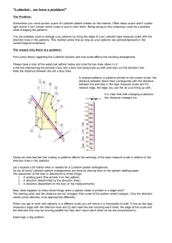
"Lutterloh... we have a problem!"
Report Card on Red Tape Reduction
Nested Virtualization State of the art and future directions Bandan Das
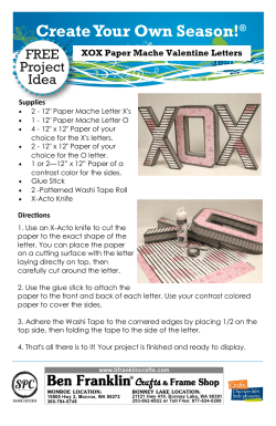
Create Your Own Season! ® XOX Paper Mache Valentine Letters
SILICONE TAPE
Spacing Tape Guide
How to Measure
Multilevel Modeling Break
Document 195973
© Copyright 2026
About abcdocz
DMCA / GDPR
Report