
11 Recursive Description of Patterns
11
CHAPTER
Recursive
Description
of Patterns
✦
✦ ✦
✦
In the last chapter, we saw two equivalent ways to describe patterns. One was
graph-theoretic, using the labels of paths in a kind of graph that we called an
“automaton.” The other was algebraic, using the regular expression notation. In
this chapter, we shall see a third way to describe patterns, using a form of recursive
definition called a “context-free grammar” (“grammar” for short).
One important application of grammars is the specification of programming
languages. Grammars are a succinct notation for describing the syntax of typical
programming languages; we shall see many examples in this chapter. Further, there
is mechanical way to turn a grammar for a typical programming language into a
“parser,” one of the key parts of a compiler for the language. The parser uncovers
the structure of the source program, often in the form of an expression tree for each
statement in the program.
✦
✦ ✦
✦
11.1
What This Chapter Is About
This chapter focuses on the following topics.
✦
Grammars and how grammars are used to define languages (Sections 11.2 and
11.3).
✦
Parse trees, which are tree representations that display the structure of strings
according to a given grammar (Section 11.4).
✦
Ambiguity, the problem that arises when a string has two or more distinct
parse trees and thus does not have a unique “structure” according to a given
grammar (Section 11.5).
✦
A method for turning a grammar into a “parser,” which is an algorithm to tell
whether a given string is in a language (Sections 11.6 and 11.7).
591
592
✦
✦
✦ ✦
✦
11.2
RECURSIVE DESCRIPTION OF PATTERNS
A proof that grammars are more powerful than regular expressions for describing languages (Section 11.8). First, we show that grammars are at least as
descriptive as regular expressions by showing how to simulate a regular expression with a grammar. Then we describe a particular language that can be
specified by a grammar, but by no regular expression.
Context-Free Grammars
Arithmetic expressions can be defined naturally by a recursive definition. The
following example illustrates how the definition works. Let us consider arithmetic
expressions that involve
1.
2.
3.
The four binary operators, +, −, ∗, and /,
Parentheses for grouping, and
Operands that are numbers.
The usual definition of such expressions is an induction of the following form:
BASIS.
A number is an expression.
INDUCTION.
a)
b)
c)
d)
e)
If E is an expression, then each of the following is also an expression:
(E). That is, we may place parentheses around an expression to get a new
expression.
E + E. That is, two expressions connected by a plus sign is an expression.
E − E. This and the next two rules are analogous to (b), but use the other
operators.
E ∗ E.
E/E.
This induction defines a language, that is, a set of strings. The basis states
that any number is in the language. Rule (a) states that if s is a string in the
language, then so is the parenthesized string (s); this string is s preceded by a left
parenthesis and followed by a right parenthesis. Rules (b) to (e) say that if s and t
are two strings in the language, then so are the strings s+t, s-t, s*t, and s/t.
Grammars allow us to write down such rules succinctly and with a precise
meaning. As an example, we could write our definition of arithmetic expressions
with the grammar shown in Fig. 11.1.
(1)
(2)
(3)
(4)
(5)
(6)
<Expression>
<Expression>
<Expression>
<Expression>
<Expression>
<Expression>
→
→
→
→
→
→
number
( <Expression> )
<Expression> + <Expression>
<Expression> – <Expression>
<Expression> * <Expression>
<Expression> / <Expression>
Fig. 11.1. Grammar for simple arithmetic expressions.
SEC. 11.2
CONTEXT-FREE GRAMMARS
593
The symbols used in Fig. 11.1 require some explanation. The symbol
<Expression>
is called a syntactic category; it stands for any string in the language of arithmetic
expressions. The symbol → means “can be composed of.” For instance, rule (2) in
Fig. 11.1 states that an expression can be composed of a left parenthesis followed by
any string that is an expression followed by a right parenthesis. Rule (3) states that
an expression can be composed of any string that is an expression, the character +,
and any other string that is an expression. Rules (4) through (6) are similar to rule
(3).
Rule (1) is different because the symbol number on the right of the arrow is
not intended to be a literal string, but a placeholder for any string that can be
interpreted as a number. We shall later show how numbers can be defined grammatically, but for the moment let us imagine that number is an abstract symbol,
and expressions use this symbol to represent any atomic operand.
Syntactic
category
The Terminology of Grammars
There are three kinds of symbols that appear in grammars. The first are “metasymbols,” symbols that play special roles and do not stand for themselves. The
only example we have seen so far is the symbol →, which is used to separate the
syntactic category being defined from a way in which strings of that syntactic category may be composed. The second kind of symbol is a syntactic category, which
as we mentioned represents a set of strings being defined. The third kind of symbol
is called a terminal. Terminals can be characters, such as + or (, or they can be
abstract symbols such as number, that stand for one or more strings we may wish
to define at a later time.
A grammar consists of one or more productions. Each line of Fig. 11.1 is a
production. In general, a production has three parts:
Metasymbol
Terminal
Production
Head and body
1.
A head, which is the syntactic category on the left side of the arrow,
2.
The metasymbol →, and
3.
A body, consisting of 0 or more syntactic categories and/or terminals on the
right side of the arrow.
For instance, in rule (2) of Fig. 11.1, the head is <Expression>, and the body
consists of three symbols: the terminal (, the syntactic category <Expression>,
and the terminal ).
✦
Example 11.1. We can augment the definition of expressions with which we
began this section by providing a definition of number. We assume that numbers
are strings consisting of one or more digits. In the extended regular-expression
notation of Section 10.6, we could say
digit = [0-9]
number = digit+
However, we can also express the same idea in grammatical notation. We could
write the productions
594
RECURSIVE DESCRIPTION OF PATTERNS
Notational Conventions
We denote syntactic categories by a name, in italics, surrounded by angular brackets,
for example, <Expression >. Terminals in productions will either be denoted by a
boldface x to stand for the string x (in analogy with the convention for regular
expressions), or by an italicized character string with no angular brackets, for the
case that the terminal, like number, is an abstract symbol.
We use the metasymbol ǫ to stand for an empty body. Thus, the production
<S> → ǫ means that the empty string is in the language of syntactic category <S>.
We sometimes group the bodies for one syntactic category into one production,
separating the bodies by the metasymbol |, which we can read as “or.” For example,
if we have productions
<S> → B1 , <S> → B2 , . . . , <S> → Bn
where the B’s are each the body of a production for the syntactic category <S>,
then we can write these productions as
<S> → B1 | B2 | · · · | Bn
<Digit > → 0 | 1 | 2 | 3 | 4 | 5 | 6 | 7 | 8 | 9
<Number> → <Digit >
<Number> → <Number> <Digit >
Note that, by our convention regarding the metasymbol |, the first line is short for
the ten productions
<Digit > → 0
<Digit > → 1
···
<Digit > → 9
We could similarly have combined the two productions for <Number> into one
line. Note that the first production for <Number > states that a single digit is a
number, and the second production states that any number followed by another
digit is also a number. These two productions together say that any string of one
or more digits is a number.
Figure 11.2 is an expanded grammar for expressions, in which the abstract
terminal number has been replaced by productions that define the concept. Notice
that the grammar has three syntactic categories, <Expression>, <Number> and
<Digit >. We shall treat the syntactic category <Expression> as the start symbol;
it generates the strings (in this case, well-formed arithmetic expressions) that we
intend to define with the grammar. The other syntactic categories, <Number> and
<Digit >, stand for auxiliary concepts that are essential, but not the main concept
for which the grammar was written. ✦
Start symbol
✦
Example 11.2. In Section 2.6 we discussed the notion of strings of balanced
parentheses. There, we gave an inductive definition of such strings that resembles,
in an informal way, the formal style of writing grammars developed in this section.
SEC. 11.2
CONTEXT-FREE GRAMMARS
595
Common Grammatical Patterns
Example 11.1 used two productions for <N umber> to say that “a number is a
string of one or more digits.” The pattern used there is a common one. In general,
if we have a syntactic category <X>, and Y is either a terminal or another syntactic
category, the productions
<X> → <X>Y | Y
say that any string of one or more Y ’s is an <X>. Adopting the regular expression
notation, <X> = Y + . Similarly, the productions
<X> → <X>Y | ǫ
tell us that every string of zero or more Y ’s is an <X>, or <X> = Y *. A slightly
more complex, but also common pattern is the pair of productions
<X> → <X>ZY | Y
which say that every string of alternating Y ’s and Z’s, beginning and ending with
a Y , is an <X>. That is, <X> = Y (ZY )*.
Moreover, we can reverse the order of the symbols in the body of the recursive
production in any of the three examples above. For instance,
<X> → Y <X> | Y
also defines <X> = Y + .
(1)
<Digit > → 0 | 1 | 2 | 3 | 4 | 5 | 6 | 7 | 8 | 9
(2)
(3)
<Number> → <Digit >
<Number> → <Number> <Digit >
(4)
(5)
(6)
(7)
(8)
(9)
<Expression>
<Expression>
<Expression>
<Expression>
<Expression>
<Expression>
→
→
→
→
→
→
<Number >
( <Expression> )
<Expression> + <Expression>
<Expression> – <Expression>
<Expression> * <Expression>
<Expression> / <Expression>
Fig. 11.2. Grammar for expressions with numbers defined grammatically.
We defined a syntactic category of “balanced parenthesis strings” that we might
call <Balanced >. There was a basis rule stating that the empty string is balanced.
We can write this rule as a production,
<Balanced > → ǫ
Then there was an inductive step that said if x and y were balanced strings, then
so was (x)y. We can write this rule as a production
<Balanced > → ( <Balanced > ) <Balanced >
Thus, the grammar of Fig. 11.3 may be said to define balanced strings of parenthe-
596
RECURSIVE DESCRIPTION OF PATTERNS
<Balanced > → ǫ
<Balanced > → ( <Balanced > ) <Balanced >
Fig. 11.3. A grammar for balanced parenthesis strings.
ses.
There is another way that strings of balanced parentheses could be defined. If
we recall Section 2.6, our original motivation for describing such strings was that
they are the subsequences of parentheses that appear within expressions when we
delete all but the parentheses. Figure 11.1 gives us a grammar for expressions.
Consider what happens if we remove all terminals but the parentheses. Production
(1) becomes
<Expression> → ǫ
Production (2) becomes
<Expression> → ( <Expression> )
and productions (3) through (6) all become
<Expression> → <Expression> <Expression>
If we replace the syntactic category <Expression> by a more appropriate name,
<BalancedE >, we get another grammar for balanced strings of parentheses, shown
in Fig. 11.4. These productions are rather natural. They say that
1.
The empty string is balanced,
2.
If we parenthesize a balanced string, the result is balanced, and
3.
The concatenation of balanced strings is balanced.
<BalancedE > → ǫ
<BalancedE > → ( <BalancedE > )
<BalancedE > → <BalancedE > <BalancedE >
Fig. 11.4. A grammar for balanced parenthesis strings
developed from the arithmetic expression grammar.
The grammars of Figs. 11.3 and 11.4 look rather different, but they do define
the same set of strings. Perhaps the easiest way to prove that they do is to show that
the strings defined by <BalancedE > in Fig. 11.4 are exactly the “profile balanced”
strings defined in Section 2.6. There, we proved the same assertion about the strings
defined by <Balanced > in Fig. 11.3. ✦
✦
Example 11.3. We can also describe the structure of control flow in languages
like C grammatically. For a simple example, it helps to imagine that there are abstract terminals condition and simpleStat. The former stands for a conditional expression. We could replace this terminal by a syntactic category, say <Condition >.
SEC. 11.2
CONTEXT-FREE GRAMMARS
597
The productions for <Condition> would resemble those of our expression grammar
above, but with logical operators like &&, comparison operators like <, and the
arithmetic operators.
The terminal simpleStat stands for a statement that does not involve nested
control structure, such as an assignment, function call, read, write, or jump statement. Again, we could replace this terminal by a syntactic category and the productions to expand it.
We shall use <Statement> for our syntactic category of C statements. One
way statements can be formed is through the while-construct. That is, if we have a
statement to serve as the body of the loop, we can precede it by the keyword while
and a parenthesized condition to form another statement. The production for this
statement-formation rule is
<Statement> → while ( condition ) <Statement>
Another way to build statements is through selection statements. These statements take two forms, depending on whether or not they have an else-part; they
are expressed by the two productions
<Statement> → if ( condition ) <Statement>
<Statement> → if ( condition ) <Statement> else <Statement>
There are other ways to form statements as well, such as for-, repeat-, and casestatements. We shall leave those productions as exercises; they are similar in spirit
to what we have seen.
However, one other important formation rule is the block, which is somewhat
different from those we have seen. A block is formed by curly braces { and },
surrounding zero or more statements. To describe blocks, we need an auxiliary
syntactic category, which we can call <StatList>; it stands for a list of statements.
The productions for <StatList> are simple:
<StatList> → ǫ
<StatList> → <StatList> <Statement>
That is, the first production says that a statement list can be empty. The second
production says that if we follow a list of statements by another statement, then we
have a list of statements.
Now we can define statements that are blocks as a statement list surrounded
by { and }, that is,
<Statement> → { <StatList> }
The productions we have developed, together with the basis production that states
that a statement can be a simple statement (assignment, call, input/output, or
jump) followed by a semicolon is shown in Fig. 11.5. ✦
EXERCISES
11.2.1: Give a grammar to define the syntactic category <Identifier>, for all those
strings that are C identifiers. You may find it useful to define some auxiliary
syntactic categories like <Digit >.
598
RECURSIVE DESCRIPTION OF PATTERNS
<Statement>
<Statement>
<Statement>
<Statement>
<Statement>
→
→
→
→
→
while ( condition ) <Statement>
if ( condition ) <Statement>
if ( condition ) <Statement> else <Statement>
{ <StatList> }
simpleStat ;
<StatList> → ǫ
<StatList> → <StatList> <Statement>
Fig. 11.5. Productions defining some of the statement forms of C.
11.2.2: Arithmetic expressions in C can take identifiers, as well as numbers, as
operands. Modify the grammar of Fig. 11.2 so that operands can also be identifiers.
Use your grammar from Exercise 11.2.1 to define identifiers.
11.2.3: Numbers can be real numbers, with a decimal point and an optional power
of 10, as well as integers. Modify the grammar for expressions in Fig. 11.2, or your
grammar from Exercise 11.2.2, to allow reals as operands.
11.2.4*: Operands of C arithmetic expressions can also be expressions involving
pointers (the * and & operators), fields of a record structure (the . and -> operators),
or array indexing. An index of an array can be any expression.
a)
Write a grammar for the syntactic category <ArrayRef > to define strings
consisting of a pair of brackets surrounding an expression. You may use the
syntactic category <Expression> as an auxiliary.
b)
Write a grammar for the syntactic category <N ame> to define strings that
refer to operands. An example of a name, as discussed in Section 1.4, is
(*a).b[c][d]. You may use <ArrayRef > as an auxiliary.
c)
Write a grammar for arithmetic expressions that allow names as operands.
You may use <N ame> as an auxiliary. When you put your productions from
(a), (b), and (c) together, do you get a grammar that allows expressions like
a[b.c][*d]+e?
11.2.5*: Show that the grammar of Fig. 11.4 generates the profile-balanced strings
defined in Section 2.6. Hint : Use two inductions on string length similar to the
proofs in Section 2.6.
11.2.6*: Sometimes expressions can have two or more kinds of balanced parentheses. For example, C expressions can have both round and square parentheses, and
both must be balanced; that is, every ( must match a ), and every [ must match
a ]. Write a grammar for strings of balanced parentheses of these two types. That
is, you must generate all and only the strings of such parentheses that could appear
in well-formed C expressions.
11.2.7: To the grammar of Fig. 11.5 add productions that define for-, do-while-,
and switch-statements. Use abstract terminals and auxiliary syntactic categories as
appropriate.
11.2.8*: Expand the abstract terminal condition in Example 11.3 to show the use
of logical operators. That is, define a syntactic category <Condition > to take the
SEC. 11.3
LANGUAGES FROM GRAMMARS
599
place of the terminal condition. You may use an abstract terminal comparison to
represent any comparison expression, such as x+1<y+z. Then replace comparison by
a syntactic category <Comparison> that expresses arithmetic comparisons in terms
of the comparison operators such as < and a syntactic category <Expression >. The
latter can be defined roughly as in the beginning of Section 11.2, but with additional
operators found in C, such as unary minus and %.
11.2.9*: Write productions that will define the syntactic category <SimpleStat >,
to replace the abstract terminal simpleStat in Fig. 11.5. You may assume the syntactic category <Expression> stands for C arithmetic expressions. Recall that a
“simple statement” can be an assignment, function call, or jump, and that, technically, the empty string is also a simple statement.
✦
✦ ✦
✦
11.3
Languages from Grammars
A grammar is essentially an inductive definition involving sets of strings. The major
departure from the examples of inductive definitions seen in Section 2.6 and many
of the examples we had in Section 11.2 is that with grammars it is routine for several
syntactic categories to be defined by one grammar. In contrast, our examples of
Section 2.6 each defined a single notion. Nonetheless, the way we constructed the set
of defined objects in Section 2.6 applies to grammars. For each syntactic category
<S> of a grammar, we define a language L(<S>), as follows:
BASIS. Start by assuming that for each syntactic category <S> in the grammar,
the language L(<S>) is empty.
INDUCTION. Suppose the grammar has a production <S> → X1 X2 · · · Xn , where
each Xi , for i = 1, 2, . . . , n, is either a syntactic category or a terminal. For each
i = 1, 2, . . . , n, select a string si for Xi as follows:
1.
If Xi is a terminal, then we may only use Xi as the string si .
2.
If Xi is a syntactic category, then select as si any string that is already known
to be in L(Xi ). If several of the Xi ’s are the same syntactic category, we can
pick a different string from L(Xi ) for each occurrence.
Then the concatenation s1 s2 · · · sn of these selected strings is a string in the language
L(<S>). Note that if n = 0, then we put ǫ in the language.
One systematic way to implement this definition is to make a sequence of rounds
through the productions of the grammar. On each round we update the language
of each syntactic category using the inductive rule in all possible ways. That is, for
each Xi that is a syntactic category, we pick strings from L(<Xi >) in all possible
ways.
✦
Example 11.4. Let us consider a grammar consisting of some of the productions
from Example 11.3, the grammar for some kinds of C statements. To simplify, we
shall only use the productions for while-statements, blocks, and simple statements,
and the two productions for statement lists. Further, we shall use a shorthand that
600
RECURSIVE DESCRIPTION OF PATTERNS
condenses the strings considerably. The shorthand uses the terminals w (while),
c (parenthesized condition), and s (simpleStat). The grammar uses the syntactic
category <S> for statements and the syntactic category <L> for statement lists.
The productions are shown in Fig. 11.6.
(1)
(2)
(3)
<S> → w c <S>
<S> → { <L> }
<S> → s ;
(4)
(5)
<L> → <L> <S>
<L> → ǫ
Fig. 11.6. Simplified grammar for statements.
Let L be the language of strings in the syntactic category <L>, and let S
be the language of strings in the syntactic category <S>. Initially, by the basis
rule, both L and S are empty. In the first round, only productions (3) and (5)
are useful, because the bodies of all the other productions each have a syntactic
category, and we do not yet have any strings in the languages for the syntactic
categories. Production (3) lets us infer that s; is a string in the language S, and
production (5) tells us that ǫ is in language L.
The second round begins with L = {ǫ}, and S = {s;}. Production (1) now
allows us to add wcs; to S, since s; is already in S. That is, in the body of
production (1), terminals w and c can only stand for themselves, but syntactic
category <S> can be replaced by any string in the language S. Since at present,
string s; is the only member of S, we have but one choice to make, and that choice
yields the string wcs;.
Production (2) adds string {}, since terminals { and } can only stand for
themselves, but syntactic category <L> can stand for any string in language L. At
the moment, L has only ǫ.
Since production (3) has a body consisting of a terminal, it will never produce
any string other than s;, so we can forget this production from now on. Similarly,
production (5) will never produce any string other than ǫ, so we can ignore it on
this and future rounds.
Finally, production (4) produces string s; for L when we replace <L> by ǫ and
replace <S> by s;. At the end of round 2, the languages are S = {s;, wcs;, {}},
and L = {ǫ, s;}.
On the next round, we can use productions (1), (2), and (4) to produce new
strings. In production (1), we have three choices to substitute for <S>, namely s;,
wcs;, and {}. The first gives us a string for language S that we already have, but
the other two give us new strings wcwcs; and wc{}.
Production (2) allows us to substitute ǫ or s; for <L>, giving us old string {}
and new string {s;} for language S. In production (4), we can substitute ǫ or s;
for <L> and s;, wcs;, or {} for <S>, giving us for language L one old string, s;,
and the five new strings wcs;, {}, s;s;, s;wcs;, and s;{}.1
1
We are being extremely systematic about the way we substitute strings for syntactic categories. We assume that throughout each round, the languages L and S are fixed as they were
defined at the end of the previous round. Substitutions are made into each of the production
bodies. The bodies are allowed to produce new strings for the syntactic categories of the
SEC. 11.3
LANGUAGES FROM GRAMMARS
601
The current languages are S = {s;, wcs;, {}, wcwcs;, wc{}, {s;}}, and
L = {ǫ, s;, wcs;, {}, s;s;, s;wcs;, s;{}}
We may proceed in this manner as long as we like. Figure 11.7 summarizes the first
three rounds. ✦
S
L
Round 1:
s;
ǫ
Round 2:
wcs;
{}
s;
Round 3:
wcwcs;
wc{}
{s;}
wcs;
{}
s;s;
s;wcs;
s;{}
Fig. 11.7. New strings on first three rounds.
Infinite
language
As in Example 11.4, the language defined by a grammar may be infinite. When
a language is infinite, we cannot list every string. The best we can do is to enumerate
the strings by rounds, as we started to do in Example 11.4. Any string in the
language will appear on some round, but there is no round at which we shall have
produced all the strings. The set of strings that would ever be put into the language
of a syntactic category <S> forms the (infinite) language L(<S>).
EXERCISES
11.3.1: What new strings are added on the fourth round in Example 11.4?
11.3.2*: On the ith round of Example 11.4, what is the length of the shortest
string that is new for either of the syntactic categories? What is the length of the
longest new string for
a)
b)
<S>
<L>?
11.3.3: Using the grammar of
a)
b)
Fig. 11.3
Fig. 11.4
generate strings of balanced parentheses by rounds. Do the two grammars generate
the same strings on the same rounds?
heads, but we do not use the strings newly constructed from one production in the body
of another production on the same round. It doesn’t matter. All strings that are going to
be generated will eventually be generated on some round, regardless of whether or not we
immediately recycle new strings into the bodies or wait for the next round to use the new
strings.
602
RECURSIVE DESCRIPTION OF PATTERNS
11.3.4: Suppose that each production with some syntactic category <S> as its
head also has <S> appearing somewhere in its body. Why is L(<S>) empty?
11.3.5*: When generating strings by rounds, as described in this section, the only
new strings that can be generated for a syntactic category <S> are found by making
a substitution for the syntactic categories of the body of some production for <S>,
such that at least one substituted string was newly discovered on the previous round.
Explain why the italicized condition is correct.
11.3.6**: Suppose we want to tell whether a particular string s is in the language
of some syntactic category <S>.
✦
✦ ✦
✦
11.4
a)
Explain why, if on some round, all the new strings generated for any syntactic
category are longer than s, and s has not already been generated for L(<S>),
then s cannot ever be put in L(<S>). Hint : Use Exercise 11.3.5.
b)
Explain why, after some finite number of rounds, we must fail to generate any
new strings that are as short as or shorter than s.
c)
Use (a) and (b) to develop an algorithm that takes a grammar, one of its
syntactic categories <S>, and a string of terminals s, and tells whether s is in
L(<S>).
Parse Trees
As we have seen, we can discover that a string s belongs to the language L(<S>),
for some syntactic category <S>, by the repeated application of productions. We
start with some strings derived from basis productions, those that have no syntactic
category in the body. We then “apply” productions to strings already derived for
the various syntactic categories. Each application involves substituting strings for
occurrences of the various syntactic categories in the body of the production, and
thereby constructing a string that belongs to the syntactic category of the head.
Eventually, we construct the string s by applying a production with <S> at the
head.
It is often useful to draw the “proof” that s is in L(<S>) as a tree, which
we call a parse tree. The nodes of a parse tree are labeled, either by terminals, by
syntactic categories, or by the symbol ǫ. The leaves are labeled only by terminals
or ǫ, and the interior nodes are labeled only by syntactic categories.
Every interior node v represents the application of a production. That is, there
must be some production such that
✦
1.
The syntactic category labeling v is the head of the production, and
2.
The labels of the children of v, from the left, form the body of the production.
Example 11.5. Figure 11.8 is an example of a parse tree, based on the grammar
of Fig. 11.2. However, we have abbreviated the syntactic categories <Expression>,
<N umber>, and <Digit> to <E>, <N >, and <D>, respectively. The string
represented by this parse tree is 3*(2+14).
For example, the root and its children represent the production
SEC. 11.4
PARSE TREES
603
<E>
<E>
*
<E>
<N >
(
<E>
)
<D>
<E>
+
<E>
3
<N >
<N >
<D>
<N >
<D>
2
<D>
4
1
Fig. 11.8. Parse tree for the string 3 ∗ (2 + 14) using the grammar from Fig. 11.2.
<E> → <E> * <E>
which is production (6) in Fig. 11.2. The rightmost child of the root and its three
children form the production <E> → (<E>), or production (5) of Fig. 11.2. ✦
Constructing Parse Trees
Yield of a tree
Each parse tree represents a string of terminals s, which we call the yield of the tree.
The string s consists of the labels of the leaves of the tree, in left-to-right order.
Alternatively, we can find the yield by doing a preorder traversal of the parse tree
and listing only the labels that are terminals. For example, the yield of the parse
tree in Fig. 11.8 is 3*(2+14).
If a tree has one node, that node will be labeled by a terminal or ǫ, because
it is a leaf. If the tree has more than one node, then the root will be labeled by
a syntactic category, since the root of a tree of two or more nodes is always an
interior node. This syntactic category will always include, among its strings, the
yield of the tree. The following is an inductive definition of the parse trees for a
given grammar.
BASIS. For every terminal of the grammar, say x, there is a tree with one node
labeled x. This tree has yield x, of course.
Suppose we have a production <S> → X1 X2 · · · Xn , where each of
the Xi ’s is either a terminal or a syntactic category. If n = 0, that is, the production
is really <S> → ǫ, then there is a tree like that of Fig. 11.9. The yield is ǫ, and
INDUCTION.
604
RECURSIVE DESCRIPTION OF PATTERNS
<S>
ǫ
Fig. 11.9. Parse tree from production <S> → ǫ.
the root is <S>; surely string ǫ is in L(<S>), because of this production.
Now suppose <S> → X1 X2 · · · Xn and n ≥ 1. We may choose a tree Ti for
each Xi , i = 1, 2, . . . , n, as follows:
1.
If Xi is a terminal, we must choose the 1-node tree labeled Xi . If two or more
of the X’s are the same terminal, then we must choose different one-node trees
with the same label for each occurrence of this terminal.
2.
If Xi is a syntactic category, we may choose any parse tree already constructed
that has Xi labeling the root. We then construct a tree that looks like Fig.
11.10. That is, we create a root labeled <S>, the syntactic category at the
head of the production, and we give it as children, the roots of the trees selected
for X1 , X2 , . . . , Xn , in order from the left. If two or more of the X’s are the
same syntactic category, we may choose the same tree for each, but we must
make a distinct copy of the tree each time it is selected. We are also permitted
to choose different trees for different occurrences of the same syntactic category.
<S>
X1
X2
T1
T2
···
Xn
Tn
Fig. 11.10. Constructing a parse tree using a production and other parse trees.
✦
Example 11.6. Let us follow the construction of the parse tree in Fig. 11.8, and
see how its construction mimics a proof that the string 3*(2+14) is in L(<E>).
First, we can construct a one-node tree for each of the terminals in the tree. Then
the group of productions on line (1) of Fig. 11.2 says that each of the ten digits is a
string of length 1 belonging to L(<D>). We use four of these productions to create
the four trees shown in Fig. 11.11. For instance, we use the production <D> →1
to create the parse tree in Fig. 11.11(a) as follows. We create a tree with a single
node labeled 1 for the symbol 1 in the body. Then we create a node labeled <D>
as the root and give it one child, the root (and only node) of the tree selected for 1.
Our next step is to use production (2) of Fig. 11.2, or <N > → <D>, to
discover that digits are numbers. For instance, we may choose the tree of Fig.
11.11(a) to substitute for <D> in the body of production (2), and get the tree of
Fig. 11.12(a). The other two trees in Fig. 11.12 are produced similarly.
SEC. 11.4
PARSE TREES
<D>
<D>
<D>
<D>
1
2
3
4
(a)
(b)
(c)
(d)
605
Fig. 11.11. Parse trees constructed using production
<D> → 1 and similar productions.
<N >
<N >
<N >
<D>
<D>
<D>
1
2
3
(a)
(b)
(c)
Fig. 11.12. Parse trees constructed using production <N > → <D>.
Now we can use production (3), which is <N > → <N ><D>. For <N > in the
body we shall select the tree of Fig. 11.12(a), and for <D> we select Fig. 11.11(d).
We create a new node labeled by <N >, for the head, and give it two children, the
roots of the two selected trees. The resulting tree is shown in Fig. 11.13. The yield
of this tree is the number 14.
<N >
<N >
<D>
<D>
4
1
Fig. 11.13. Parse trees constructed using production <N > → <N ><D>.
Our next task is to create a tree for the sum 2+14. First, we use the production
(4), or <E> → <N >, to build the parse trees of Fig. 11.14. These trees show that
3, 2, and 14 are expressions. The first of these comes from selecting the tree of Fig.
11.12(c) for <N > of the body. The second is obtained by selecting the tree of Fig.
11.12(b) for <N >, and the third by selecting the tree of Fig. 11.13.
Then we use production (6), which is <E> → <E>+<E>. For the first <E>
in the body we use the tree of Fig. 11.14(b), and for the second <E> in the body
we use the tree of Fig. 11.14(c). For the terminal + in the body, we use a one-node
tree with label +. The resulting tree is shown in Fig. 11.15; its yield is 2+14.
606
RECURSIVE DESCRIPTION OF PATTERNS
<E>
<E>
<E>
<N >
<N >
<N >
<D>
<D>
<N >
<D>
3
2
<D>
4
(a)
(b)
1
(c)
Fig. 11.14. Parse trees constructed using production <E> → <N >.
<E>
<E>
<E>
+
<N >
<N >
<D>
<N >
<D>
2
<D>
4
1
Fig. 11.15. Parse tree constructed using production <E> → <E>+<E>.
We next use production (5), or <E> → (<E>), to construct the parse tree of
Fig. 11.16. We have simply selected the parse tree of Fig. 11.15 for the <E> in the
body, and we select the obvious one-node trees for the terminal parentheses.
Lastly, we use production (8), which is <E> → <E> * <E>, to construct the
parse tree that we originally showed in Fig. 11.8. For the first <E> in the body,
we choose the tree of Fig. 11.14(a), and for the second we choose the tree of Fig.
11.16. ✦
Why Parse Trees “Work”
The construction of parse trees is very much like the inductive definition of the
strings belonging to a syntactic category. We can prove, by two simple inductions,
that the yields of the parse trees with root <S> are exactly the strings in L(<S>),
for any syntactic category <S>. That is,
SEC. 11.4
PARSE TREES
607
<E>
(
<E>
)
<E>
+
<E>
<N >
<N >
<D>
<N >
<D>
2
<D>
4
1
Fig. 11.16. Parse tree constructed using production <E> → (<E>).
1.
If T is a parse tree with root labeled <S> and yield s, then string s is in the
language L(<S>).
2.
If string s is in L(<S>), then there is a parse tree with yield s and root labeled
<S>.
This equivalence should be fairly intuitive. Roughly, parse trees are assembled from
smaller parse trees in the same way that we assemble long strings from shorter ones,
using substitution for syntactic categories in the bodies of productions. We begin
with part (1), which we prove by complete induction on the height of tree T .
Suppose the height of the parse tree is 1. Then the tree looks like Fig. 11.17,
or, in the special case where n = 0, like the tree of Fig. 11.9. The only way we can
construct such a tree is if there is a production <S> → x1 x2 · · · xn , where each of
the x’s is a terminal (if n = 0, the production is <S> → ǫ). Thus, x1 x2 · · · xn is a
string in L(<S>).
BASIS.
<S>
x1
x2
···
xn
Fig. 11.17. Parse tree of height 1.
608
RECURSIVE DESCRIPTION OF PATTERNS
INDUCTION. Suppose that statement (1) holds for all trees of height k or less.
Now consider a tree of height k + 1 that looks like Fig. 11.10. Then each of the
subtrees Ti , for i = 1, 2, . . . , n, can be of height at most k. For if any one of the
subtrees had height k + 1 or more, the entire tree would have height at least k + 2.
Thus, the inductive hypothesis applies to each of the trees Ti .
By the inductive hypothesis, if Xi , the root of the subtree Ti , is a syntactic
category, then the yield of Ti , say si , is in the language L(Xi ). If Xi is a terminal,
let us define string si to be Xi . Then the yield of the entire tree is s1 s2 · · · sn .
We know that <S> → X1 X2 · · · Xn is a production, by the definition of a
parse tree. Suppose that we substitute string si for Xi , whenever Xi is a syntactic
category. By definition, Xi is si if Xi is a terminal. It follows that the substituted
body is s1 s2 · · · sn , the same as the yield of the tree. By the inductive rule for the
language of <S>, we know that s1 s2 · · · sn is in L(<S>).
Now we must prove statement (2), that every string s in a syntactic category
<S> has a parse tree with root <S> and s as yield. To begin, let us note that
for each terminal x, there is a parse tree with both root and yield x. Now we use
complete induction on the number of times we applied the inductive step (described
in Section 11.3) when we deduced that s is in L(<S>).
Suppose s requires one application of the inductive step to show that s is
in L(<S>). Then there must be a production <S> → x1 x2 · · · xn , where all the
x’s are terminals, and s = x1 x2 · · · xn . We know that there is a one node parse
tree labeled xi for i = 1, 2, . . . , n. Thus, there is a parse tree with yield s and root
labeled <S>; this tree looks like Fig. 11.17. In the special case that n = 0, we know
s = ǫ, and we use the tree of Fig. 11.9 instead.
BASIS.
INDUCTION. Suppose that any string t found to be in the language of any syntactic
category <T > by k or fewer applications of the inductive step has a parse tree with
t as yield and <T > at the root. Consider a string s that is found to be in the
language of syntactic category <S> by k + 1 applications of the inductive step.
Then there is a production <S> → X1 X2 · · · Xn , and s = s1 s2 · · · sn , where each
substring si is either
1.
Xi , if Xi is a terminal, or
2.
Some string known to be in L(Xi ) using at most k applications of the inductive
rule, if Xi is a syntactic category.
Thus, for each i, we can find a tree Ti , with yield si and root labeled Xi . If Xi is a
syntactic category, we invoke the inductive hypothesis to claim that Ti exists, and
if Xi is a terminal, we do not need the inductive hypothesis to claim that there is
a one-node tree labeled Xi . Thus, the tree constructed as in Fig. 11.10 has yield s
and root labeled <S>, proving the induction step.
EXERCISES
11.4.1: Find a parse tree for the strings
SEC. 11.4
PARSE TREES
609
Syntax Trees and Expression Trees
Often, trees that look like parse trees are used to represent expressions. For instance,
we used expression trees as examples throughout Chapter 5. Syntax tree is another
name for “expression tree.” When we have a grammar for expressions such as
that of Fig. 11.2, we can convert parse trees to expression trees by making three
transformations:
1.
Atomic operands are condensed to a single node labeled by that operand.
2.
Operators are moved from leaves to their parent node. That is, an operator
symbol such as + becomes the label of the node above it that was labeled by
the “expression” syntactic category.
3.
Interior nodes that remain labeled by “expression” have their label removed.
For instance, the parse tree of Fig. 11.8 is converted to the following expression tree
or syntax tree:
*
3
(
2
a)
b)
c)
+
)
14
35+21
123-(4*5)
1*2*(3-4)
according to the grammar of Fig. 11.2. The syntactic category at the root should
be <E> in each case.
11.4.2: Using the statement grammar of Fig. 11.6, find parse trees for the following
strings:
a)
b)
c)
wcwcs;
{s;}
{s;wcs;}.
The syntactic category at the root should be <S> in each case.
11.4.3: Using the balanced parenthesis grammar of Fig. 11.3, find parse trees for
the following strings:
a)
b)
(()())
((()))
610
c)
RECURSIVE DESCRIPTION OF PATTERNS
((())()).
11.4.4: Find parse trees for the strings of Exercise 11.4.3, using the grammar of
Fig. 11.4.
✦
✦ ✦
✦
11.5
Ambiguity and the Design of Grammars
Let us consider the grammar for balanced parentheses that we originally showed in
Fig. 11.4, with syntactic category <B> abbreviating <Balanced >:
<B> → (<B>) | <B><B> | ǫ
(11.1)
Suppose we want a parse tree for the string ()()(). Two such parse trees are shown
in Fig. 11.18, one in which the first two pairs of parentheses are grouped first, and
the other in which the second two pairs are grouped first.
<B>
<B>
<B>
<B>
(
<B>
<B>
)
(
(
<B>
ǫ
)
<B>
)
ǫ
ǫ
(a) Parse tree that groups from the left.
<B>
<B>
(
<B>
ǫ
<B>
)
<B>
(
<B>
<B>
)
(
ǫ
<B>
ǫ
(b) Parse tree that groups from the right.
Fig. 11.18. Two parse trees with the same yield and root.
)
SEC. 11.5
Ambiguous
grammar
AMBIGUITY AND THE DESIGN OF GRAMMARS
611
It should come as no surprise that these two parse trees exist. Once we establish that both () and ()() are balanced strings of parentheses, we can use the
production <B> → <B><B> with () substituting for the first <B> in the body
and ()() substituting for the second, or vice-versa. Either way, the string ()()()
is discovered to be in the syntactic category <B>.
A grammar in which there are two or more parse trees with the same yield and
the same syntactic category labeling the root is said to be ambiguous. Notice that
not every string has to be the yield of several parse trees; it is sufficient that there
be even one such string, to make the grammar ambiguous. For example, the string
()()() is sufficient for us to conclude that the grammar (11.1) is ambiguous. A
grammar that is not ambiguous is called unambiguous. In an unambiguous grammar, for every string s and syntactic category <S>, there is at most one parse tree
with yield s and root labeled <S>.
An example of an unambiguous grammar is that of Fig. 11.3, which we reproduce here with <B> in place of <Balanced >,
<B> → (<B>)<B> | ǫ
(11.2)
A proof that the grammar is unambiguous is rather difficult. In Fig. 11.19 is the
unique parse tree for string ()()(); the fact that this string has a unique parse tree
does not prove the grammar (11.2) is unambiguous, of course. We can only prove
unambiguity by showing that every string in the language has a unique parse tree.
<B>
(
<B>
)
<B>
ǫ
(
<B>
)
<B>
ǫ
(
<B>
ǫ
)
<B>
ǫ
Fig. 11.19. Unique parse tree for the string ( ) ( ) ( ) using the grammar (11.2).
Ambiguity in Expressions
While the grammar of Fig. 11.4 is ambiguous, there is no great harm in its ambiguity,
because whether we group several strings of balanced parentheses from the left or
the right matters little. When we consider grammars for expressions, such as that
of Fig. 11.2 in Section 11.2, some more serious problems can occur. Specifically,
some parse trees imply the wrong value for the expression, while others imply the
correct value.
612
RECURSIVE DESCRIPTION OF PATTERNS
Why Unambiguity Is Important
The parser, which constructs parse trees for programs, is an essential part of a
compiler. If a grammar describing a programming language is ambiguous, and if its
ambiguities are left unresolved, then for at least some programs there is more than
one parse tree. Different parse trees for the same program normally impart different
meanings to the program, where “meaning” in this case is the action performed by
the machine language program into which the original program is translated. Thus,
if the grammar for a program is ambiguous, a compiler cannot properly decide which
parse tree to use for certain programs, and thus cannot decide what the machinelanguage program should do. For this reason, compilers must use specifications that
are unambiguous.
✦
Example 11.7. Let us use the shorthand notation for the expression grammar
that was developed in Example 11.5. Then consider the expression 1-2+3. It has
two parse trees, depending on whether we group operators from the left or the right.
These parse trees are shown in Fig. 11.20(a) and (b).
<E>
<E>
<E>
+
<E>
<E>
−
<E>
−
<E>
<N >
<N >
<E>
+
<N >
<N >
<D>
<D>
<N >
<N >
<D>
<D>
3
1
<D>
<D>
1
2
2
3
<E>
(a) Correct parse tree.
<E>
(b) Incorrect parse tree.
Fig. 11.20. Two parse trees for the expression 1 − 2 + 3.
The tree of Fig. 11.20(a) associates from the left, and therefore groups the
operands from the left. That grouping is correct, since we generally group operators
at the same precedence from the left; 1-2+3 is conventionally interpreted as (12)+3, which has the value 2. If we evaluate the expressions represented by subtrees,
working up the tree of Fig. 11.20(a), we first compute 1 − 2 = −1 at the leftmost
child of the root, and then compute −1 + 3 = 2 at the root.
On the other hand, Fig. 11.20(b), which associates from the right, groups our
expression as 1-(2+3), whose value is −4. This interpretation of the expression
is unconventional, however. The value −4 is obtained working up the tree of Fig.
SEC. 11.5
AMBIGUITY AND THE DESIGN OF GRAMMARS
613
11.20(b), since we evaluate 2 + 3 = 5 at the rightmost child of the root, and then
1 − 5 = −4 at the root. ✦
Associating operators of equal precedence from the wrong direction can cause
problems. We also have problems with operators of different precedence; it is possible to group an operator of low precedence before one of higher precedence, as we
see in the next example.
✦
Example 11.8. Consider the expression 1+2*3. In Fig. 11.21(a) we see the
expression incorrectly grouped from the left, while in Fig. 11.21(b), we have correctly
grouped the expression from the right, so that the multiplication gets its operands
grouped before the addition. The former grouping yields the erroneous value 9,
while the latter grouping produces the conventional value of 7. ✦
<E>
<E>
<E>
∗
<E>
<E>
+
<E>
+
<E>
<N >
<N >
<E>
∗
<N >
<N >
<D>
<D>
<N >
<N >
<D>
<D>
3
1
<D>
<D>
1
2
2
3
<E>
(a) Incorrect parse tree.
<E>
(b) Correct parse tree.
Fig. 11.21. Two parse trees for the expression 1+2*3.
Unambiguous Grammars for Expressions
Just as the grammar (11.2) for balanced parentheses can be viewed as an unambiguous version of the grammar (11.1), it is possible to construct an unambiguous
version of the expression grammar from Example 11.5. The “trick” is to define
three syntactic categories, with intuitive meanings as follows.
1.
<Factor > generates expressions that cannot be “pulled apart,” that is, a factor
is either a single operand or any parenthesized expression.
2.
<Term> generates a product or quotient of factors. A single factor is a term,
and thus is a sequence of factors separated by the operators ∗ or /. Examples
of terms are 12 and 12/3*45.
614
3.
RECURSIVE DESCRIPTION OF PATTERNS
<Expression> generates a sum or difference of one or more terms. A single term
is an expression, and thus is a sequence of terms separated by the operators +
or −. Examples of expressions are 12, 12/3*45, and 12+3*45-6.
Figure 11.22 is a grammar that expresses the relationship between expressions,
terms, and factors. We use shorthands <E>, <T >, and <F > for <Expression>,
<Term>, and <Factor >, respectively.
(1)
<E> → <E> + <T > | <E> − <T > | <T >
(2)
<T > → <T > ∗ <F > | <T >/<F > | <F >
(3)
<F > → (<E>) | <N >
(4)
<N > → <N ><D> | <D>
(5)
<D> → 0 | 1 | · · · | 9
Fig. 11.22. Unambiguous grammar for arithmetic expressions.
For instance, the three productions in line (1) define an expression to be either
a smaller expression followed by a + or - and another term, or to be a single term.
If we put these ideas together, the productions say that every expression is a term,
followed by zero or more pairs, each pair consisting of a + or - and a term. Similarly,
line (2) says that a term is either a smaller term followed by * or / and a factor, or it
is a single factor. That is, a term is a factor followed by zero or more pairs, each pair
consisting of a * or a / and a factor. Line (3) says that factors are either numbers,
or expressions surrounded by parentheses. Lines (4) and (5) define numbers and
digits as we have done previously.
The fact that in lines (1) and (2) we use productions such as
<E> → <E> + <T >
rather than the seemingly equivalent <E> → <T > + <E>, forces terms to be
grouped from the left. Thus, we shall see that an expression such as 1-2+3 is
correctly grouped as (1-2)+3. Likewise, terms such as 1/2*3 are correctly grouped
as (1/2)*3, rather than the incorrect 1/(2*3). Figure 11.23 shows the only possible
parse tree for the expression 1-2+3 in the grammar of Fig. 11.22. Notice that 1-2
must be grouped as an expression first. If we had grouped 2+3 first, as in Fig.
11.20(b), there would be no way, in the grammar of Fig. 11.22, to attach the 1- to
this expression.
The distinction among expressions, terms, and factors enforces the correct
grouping of operators at different levels of precedence. For example, the expression 1+2*3 has only the parse tree of Fig. 11.24, which groups the subexpression
2*3 first, like the tree of Fig. 11.21(b) and unlike the incorrect tree of Fig. 11.21(a),
which groups 1+2 first.
As for the matter of balanced parentheses, we have not proved that the grammar of Fig. 11.22 is unambiguous. The exercises contain a few more examples that
should help convince the reader that this grammar is not only unambiguous, but
gives the correct grouping for each expression. We also suggest how the idea of this
grammar can be extended to more general families of expressions.
SEC. 11.5
AMBIGUITY AND THE DESIGN OF GRAMMARS
<E>
<E>
+
<T >
−
<T >
<F >
<T >
<F >
<N >
<F >
<N >
<D>
<N >
<D>
3
<D>
2
<E>
1
Fig. 11.23. Parse tree for the expression 1 − 2 + 3 in the
unambiguous grammar of Fig. 11.22.
<E>
<E>
+
<T >
<T >
<T >
∗
<F >
<F >
<N >
<N >
<N >
<D>
<D>
<D>
3
1
2
<F >
Fig. 11.24. Parse tree for 1 + 2 ∗ 3 in the unambiguous grammar of Fig. 11.22.
615
616
RECURSIVE DESCRIPTION OF PATTERNS
EXERCISES
11.5.1: In the grammar of Fig. 11.22, give the unique parse tree for each of the
following expressions:
a)
b)
c)
(1+2)/3
1*2-3
(1+2)*(3+4)
11.5.2*: The expressions of the grammar in Fig. 11.22 have two levels of precedence;
+ and − at one level, and ∗ and / at a second, higher level. In general, we can handle
expressions with k levels of precedence by using k + 1 syntactic categories. Modify
the grammar of Fig. 11.22 to include the exponentiation operator ^, which is at a
level of precedence higher than * and /. As a hint, define a primary to be an operand
or a parenthesized expression, and redefine a factor to be one or more primaries
connected by the exponentiation operator. Note that exponentiation groups from
the right, not the left, and 2^3^4 means 2^(3^4), rather than (2^3)^4. How do
we force grouping from the right among primaries?
11.5.3*: Extend the unambiguous expression grammar to allow the comparison
operators, =, <=, and so on, which are all at the same level of precedence and
left-associative. Their precedence is below that of + and −.
11.5.4: Extend the expression grammar of Fig. 11.22 to include the unary minus
sign. Note that this operator is at a higher precedence than the other operators;
for instance, -2*-3 is grouped (-2)*(-3).
11.5.5: Extend your grammar of Exercise 11.5.3 to include the logical operators
&&, ||, and !. Give && the precedence of *, || the precedence of +, and ! a higher
precedence than unary −. && and || are binary operators that group from the left.
11.5.6*: Not every expression has more than one parse tree according to the ambiguous grammar of Fig. 11.2 in Section 11.2. Give several examples of expressions
that have unique parse trees according to this grammar. Can you give a rule indicating when an expression will have a unique parse tree?
11.5.7: The following grammar defines the set of strings (other than ǫ) consisting
of 0’s and 1’s only.
<String> → <String><String> | 0 | 1
In this grammar, how many parse trees does the string 010 have?
11.5.8: Give an unambiguous grammar that defines the same language as the
grammar of Exercise 11.5.7.
11.5.9*: How many parse trees does grammar (11.1) have for the empty string?
Show three different parse trees for the empty string.
✦
✦ ✦
✦
11.6
Constructing Parse Trees
Grammars are like regular expressions, in that both notations describe languages
but do not give directly an algorithm for determining whether a string is in the
SEC. 11.6
CONSTRUCTING PARSE TREES
617
language being defined. For regular expressions, we learned in Chapter 10 how to
convert a regular expression first into a nondeterministic automaton and then into
a deterministic one; the latter can be implemented directly as a program.
There is a somewhat analogous process for grammars. We cannot, in general,
convert a grammar to a deterministic automaton at all; the next section discusses
some examples of when that conversion is impossible. However, it is often possible
to convert a grammar to a program that, like an automaton, reads the input from
beginning to end and renders a decision whether the input string is in the language
of the grammar. The most important such technique, called “LR parsing” (the LR
stands for left-to-right on the input), is beyond the scope of this book.
Recursive-Descent Parsing
What we shall give instead is a simpler but less powerful parsing technique called
“recursive descent,” in which the grammar is replaced by a collection of mutually
recursive functions, each corresponding to one of the syntactic categories of the
grammar. The goal of the function S that corresponds to the syntactic category
<S> is to read a sequence of input characters that form a string in the language
L(<S>), and to return a pointer to the root of a parse tree for this string.
A production’s body can be thought of as a sequence of goals — the terminals
and syntactic categories — that must be fulfilled in order to find a string in the
syntactic category of the head. For instance, consider the unambiguous grammar
for balanced parentheses, which we reproduce here as Fig. 11.25.
(1)
(2)
<B> → ǫ
<B> → ( <B> ) <B>
Fig. 11.25. Grammar for balanced parentheses.
Production (2) states that one way to find a string of balanced parentheses is
to fulfill the following four goals in order.
Endmarker
1.
Find the character (, then
2.
3.
4.
Find a string of balanced parentheses, then
Find the character ), and finally
Find another string of balanced parentheses.
In general, a terminal goal is satisfied if we find that this terminal is the next input
symbol, but the goal cannot be satisfied if the next input symbol is something else.
To tell whether a syntactic category in the body is satisfied, we call a function for
that syntactic category.
The arrangement for constructing parse trees according to a grammar is suggested in Fig. 11.26. Suppose we want to determine whether the sequence of terminals X1 X2 · · · Xn is a string in the syntactic category <S>, and to find its parse
tree if so. Then on the input file we place X1 X2 · · · Xn ENDM, where ENDM is a special
symbol that is not a terminal.2 We call ENDM, the endmarker, and its purpose is to
2
In real compilers for programming languages, the entire input might not be placed in a file
at once, but terminals would be discovered one at a time by a preprocessor called a “lexical
analyzer” that examines the source program one character at a time.
618
RECURSIVE DESCRIPTION OF PATTERNS
indicate that the entire string being examined has been read. For example, in C
programs it would be typical to use the end-of-file or end-of-string character for the
endmarker.
X1
X2
···
Xn
ENDM
↑
Call S
Fig. 11.26. Initializing the program to discover an <S> on the input.
Input cursor
An input cursor marks the terminal to be processed, the current terminal. If
the input is a string of characters, then the cursor might be a pointer to a character.
We start our parsing program by calling the function S for the starting syntactic
category <S>, with the input cursor at the beginning of the input.
Each time we are working on a production body, and we come to a terminal a
in the production, we look for the matching terminal a at the position indicated by
the input cursor. If we find a, we advance the input cursor to the next terminal on
the input. If the current terminal is something other than a, then we fail to match,
and we cannot find a parse tree for the input string.
On the other hand, if we are working on a production body and we come to
a syntactic category <T >, we call the function T for <T >. If T “fails,” then the
entire parse fails, and the input is deemed not to be in the language being parsed.
If T succeeds, then it “consumes” some input, but moving the input cursor forward
zero or more positions on the input. All input positions, from the position at the
time T was called, up to but not including the position at which T leaves the cursor,
are consumed. T also returns a tree, which is the parse tree for the consumed input.
When we have succeeded with each of the symbols in a production body, we
assemble the parse tree for the portion of the input represented by that production.
To do so, we create a new root node, labeled by the head of the production. The
root’s children are the roots of the trees returned by successful calls to functions for
the syntactic categories of the body and leaves created for each of the terminals of
the body.
A Recursive-Descent Parser for Balanced Parentheses
Let us consider an extended example of how we might design the recursive function
B for the syntactic category <B> of the grammar of Fig. 11.25. B, called at
some input position, will consume a string of balanced parentheses starting at that
position and leave the input cursor at the position immediately after the balanced
string.
The hard part is deciding whether to satisfy the goal of finding a <B> by using
production (1), <B> → ǫ, which succeeds immediately, or by using production (2),
that is,
<B> → (<B>)<B>
The strategy we shall follow is that whenever the next terminal is (, use production
(2); whenever the next terminal is ) or the endmarker, use production (1).
The function B is given in Fig. 11.27(b). It is preceded by important auxiliary
elements in Fig. 11.27(a). These elements include:
SEC. 11.6
CONSTRUCTING PARSE TREES
#define FAILED NULL
typedef struct NODE *TREE;
struct NODE {
char label;
TREE leftmostChild, rightSibling;
};
TREE
TREE
TREE
TREE
makeNode0(char x);
makeNode1(char x, TREE t);
makeNode4(char x, TREE t1, TREE t2, TREE t3, TREE t4);
B();
TREE parseTree; /* holds the result of the parse */
char *nextTerminal; /* current position in input string */
void main()
{
nextTerminal = "()()"; /* in practice, a string
of terminals would be read from input */
parseTree = B();
}
TREE makeNode0(char x)
{
TREE root;
root = (TREE) malloc(sizeof(struct NODE));
root->label = x;
root->leftmostChild = NULL;
root->rightSibling = NULL;
return root;
}
TREE makeNode1(char x, TREE t)
{
TREE root;
root = makeNode0(x);
root->leftmostChild = t;
return root;
}
TREE makeNode4(char x, TREE t1, TREE t2, TREE t3, TREE t4)
{
TREE root;
root = makeNode1(x, t1);
t1->rightSibling = t2;
t2->rightSibling = t3;
t3->rightSibling = t4;
return root;
}
Fig. 11.27(a). Auxiliary functions for recursive-descent parser.
619
620
(1)
RECURSIVE DESCRIPTION OF PATTERNS
TREE B()
{
TREE firstB, secondB;
(2)
(3)
(4)
(5)
(6)
(7)
(8)
(9)
if(*nextTerminal == ’(’) /* follow production 2 */ {
nextTerminal++;
firstB = B();
if(firstB != FAILED && *nextTerminal == ’)’) {
nextTerminal++;
secondB = B();
if(secondB == FAILED)
return FAILED;
else
return makeNode4(’B’,
makeNode0(’(’),
firstB,
makeNode0(’)’),
secondB);
}
else /* first call to B failed */
return FAILED;
}
else /* follow production 1 */
return makeNode1(’B’, makeNode0(’e’));
(10)
(11)
(12)
}
Fig. 11.27(b). Function to construct parse trees for strings of balanced parentheses.
1.
Definition of a constant FAILED to be the value returned by B when that
function fails to find a string of balanced parentheses on the input. The value
of FAILED is the same as NULL. The latter value also represents an empty tree.
However, the parse tree returned by B could not be empty if B succeeds, so
there is no possible ambiguity in this definition of FAILED.
2.
Definitions of the types NODE and TREE. A node consists of a label field, which
is a character, and pointers to the leftmost child and right sibling. The label
may be ’B’ to represent a node labeled B, ’(’ and ’)’ to represent nodes
labeled with left- or right-parentheses, respectively, and ’e’ to represent a
node labeled ǫ. Unlike the leftmost-child-right-sibling structure of Section 5.3,
we have elected to use TREE rather than pNODE as the type of pointers to nodes
since most uses of these pointers here will be as representations of trees.
3.
Prototype declarations for three auxiliary functions to be described below and
the function B.
4.
Two global variables. The first, parseTree, holds the parse tree returned by the
initial call to B. The second, nextTerminal, is the input cursor and points to
the current position on the input string of terminals. Note that it is important
for nextTerminal to be global, so when one call to B returns, the place where
it left the input cursor is known to the copy of B that made the call.
SEC. 11.6
CONSTRUCTING PARSE TREES
621
5.
The function main. In this simple demonstration, main sets nextTerminal to
point to the beginning of a particular test string, ()(), and the result of a call
to B is placed in parseTree.
6.
Three auxiliary functions that create tree nodes and, if necessary, combine
subtrees to form larger trees. These are:
a)
Function makeNode0(x) creates a node with zero children, that is, a leaf,
and labels that leaf with the symbol x. The tree consisting of this one
node is returned.
b)
Function makeNode1(x, t) creates a node with one child. The label of the
new node is x, and the child is the root of the tree t. The tree whose root
is the created node is returned. Note that makeNode1 uses makeNode0 to
create the root node and then makes the root of tree t be the leftmost child
of the root. We assume that all leftmost-child and right-sibling pointers are
NULL initially, as they will be because they are all created by makeNode0,
which explicitly NULL’s them. Thus, it is not mandatory that makeNode1
to store NULL in the rightSibling field of the root of t, but it would be a
wise safety measure to do so.
c)
Function makeNode4(x, t1 , t2 , t3 , t4 ) creates a node with four children. The
label of the node is x, and the children are the roots of the trees t1 , t2 , t3 ,
and t4 , from the left. The tree whose root is the created node is returned.
Note that makeNode4 uses makeNode1 to create a new root and attach t1
to it, then strings the remaining trees together with right-sibling pointers.
Now we can consider the program of Fig. 11.27(b) line by line. Line (1) is
the declaration of two local variables, firstB and secondB, to hold the parse trees
returned by the two calls to B in the case that we elect to try production (2). Line
(2) tests if the next terminal on the input is (. If so, we shall look for an instance
of the body of production (2), and if not, then we shall assume that production (1)
is used, and that ǫ is the balanced string.
At line (3), we increment nextTerminal, because the current input ( has
matched the ( in the body of production (2). We now have the input cursor properly positioned for a call to B that will find a balanced string for the first <B> in
the body of production (2). That call occurs at line (4), and the tree returned is
stored in variable firstB to be assembled later into a parse tree for the current call
to B.
At line (5) we check that we are still capable of finding a balanced string. That
is, we first check that the call to B on line (4) did not fail. Then we test that the
current value of nextTerminal is ). Recall that when B returns, nextTerminal
points to the next input terminal to be formed into a balanced string. If we are to
match the body of production (2), and we have already matched the ( and the first
<B>, then we must next match the ), which explains the second part of the test.
If either part of the test fails, then the current call to B fails at line (11).
If we pass the test of line (5), then at lines (6) and (7) we advance the input
cursor over the right parenthesis just found and call B again, to match the final
<B> in production (2). The tree returned is stored temporarily in secondB.
If the call to B on line (7) fails, then secondB will have value FAILED. Line (8)
detects this condition, and the current call to B also fails.
Line (10) covers the case in which we have succeeded in finding a balanced
622
RECURSIVE DESCRIPTION OF PATTERNS
string. We return a tree constructed by makeNode4. This tree has a root labeled
’B’, and four children. The first child is a leaf labeled (, constructed by makeNode0.
The second is the tree we stored in firstB, which is the parse tree produced by the
call to B at line (4). The third child is a leaf labeled ), and the fourth is the parse
tree stored in secondB, which was returned by the second call to B at line (7).
Line (11) is used only when the test of line (5) fails. Finally, line (12) handles
the case where the original test of line (1) fails to find ( as the first character. In
that case, we assume that production (1) is correct. This production has the body
ǫ, and so we consume no input but return a node, created by makeNode1, that has
the label B and one child labeled ǫ.
✦
Example 11.9. Suppose we have the terminals ( ) ( ) ENDM on the input.
Here, ENDM stands for the character ’\0’, which marks the end of character strings
in C. The call to B from main in Fig. 11.27(a) finds ( as the current input, and the
test of line (2) succeeds. Thus, nextTerminal advances at line (3), and at line (4)
a second call to B is made, as suggested by “call 2” in Fig. 11.28.
(
)
(
)
ENDM
call 4 call 5
call 2
call 3
call 1
Fig. 11.28. Calls made while processing the input ( ) ( ) ENDM.
In call 2, the test of line (2) fails, and we thus return the tree of Fig. 11.29(a)
at line (12). Now we return to call 1, where we are at line (5), with ) pointed to
by nextTerminal and the tree of Fig. 11.29(a) in firstB. Thus, the test of line (5)
succeeds. We advance nextTerminal at line (6) and call B at line (7). This is “call
3” in Fig. 11.28.
In call 3 we succeed at line (2), advance nextTerminal at line (3), and call B
at line (4); this call is “call 4” in Fig. 11.28. As with call 2, call 4 fails the test of
line (2) and returns a (distinct) tree like that of Fig. 11.29(a) at line (12).
We now return to call 3, with nextTerminal still pointing to ), with firstB
(local to this call of B) holding a tree like Fig. 11.29(a), and with control at line
(5). The test succeeds, and we advance nextTerminal at line (6), so it now points
to ENDM. We make the fifth call to B at line (7). This call has its test fail at line (2)
and returns another copy of Fig. 11.29(a) at line (12). This tree becomes the value
of secondB for call 3, and the test of line (8) fails. Thus, at line (10) of call 3, we
construct the tree shown in Fig. 11.29(b).
At this point, call 3 returns successfully to call 1 at line (8), with secondB
of call 1 holding the tree of Fig. 11.29(b). As in call 3, the test of line (8) fails,
and at line (10) we construct a tree with a new root node, whose second child is a
copy of the tree in Fig. 11.29(a) — this tree was held in firstB of call 1 — and
whose fourth child is the tree of Fig. 11.29(b). The resulting tree, which is placed
in parseTree by main, is shown in Fig. 11.29(c). ✦
SEC. 11.6
B
CONSTRUCTING PARSE TREES
623
B
ǫ
(
B
)
B
(a)
ǫ
ǫ
(b)
B
(
B
)
B
ǫ
(
B
)
ǫ
B
ǫ
(c)
Fig. 11.29. Trees constructed by recursive calls to B.
Constructing Recursive-Descent Parsers
Lookahead
symbol
We can generalize the technique used in Fig. 11.27 to many grammars, although
not to all grammars. The key requirement is that for each syntactic category <S>,
if there is more than one production with <S> as the head, then by looking at only
the current terminal (often called the lookahead symbol), we can decide on the one
production for <S> that needs to be tried. For instance, in Fig. 11.27, our decision
strategy is to pick the second production, with body (<B>)<B>, whenever the
lookahead symbol is (, and to pick the first production, with body ǫ, when the
lookahead symbol is ) or ENDM.
It is not possible to tell, in general, whether there is an algorithm for a given
grammar that will always make the right decision. For Fig. 11.27, we claimed, but
did not prove, that the strategy stated above will work. However, if we have a
decision strategy that we believe will work, then for each syntactic category <S>,
we can design the function S to do the following:
1.
Examine the lookahead symbol and decide which production to try. Suppose
the chosen production has body X1 X2 · · · Xn .
2.
For i = 1, 2, . . . , n do the following with Xi .
a)
If Xi is a terminal, check that the lookahead symbol is Xi . If so, advance
the input cursor. If not, then this call to S fails.
b)
If Xi is a syntactic category, such as <T >, then call the function T corresponding to this syntactic category. If T returns with failure, then the
call to S fails. If T returns successfully, store away the returned tree for
use later.
624
RECURSIVE DESCRIPTION OF PATTERNS
If we have not failed after considering all the Xi ’s, then assemble a parse tree to
return by creating a new node, with children corresponding to X1 , X2 , . . . , Xn ,
in order. If Xi is a terminal, then the child for Xi is a newly created leaf with
label Xi . If Xi is a syntactic category, then the child for Xi is the root of
the tree that was returned when a call to the function for Xi was completed.
Figure 11.29 was an example of this tree construction.
If the syntactic category <S> represents the language whose strings we want
to recognize and parse, then we start the parsing process by placing the input cursor
at the first input terminal. A call to the function S will cause a parse tree for the
input to be constructed if there is one and will return failure if the input is not in
the language L(<S>).
EXERCISES
11.6.1: Show the sequence of calls made by the program of Fig. 11.27 on the inputs
a)
b)
c)
(())
(()())
())(
in each case followed by the endmarker symbol ENDM.
11.6.2: Consider the following grammar for numbers.
<Number> → <Digit ><Number> | ǫ
<Digit > → 0 | 1 | · · · | 9
Design a recursive-descent parser for this grammar; that is, write a pair of functions,
one for <Number > and the other for <Digit >. You may follow the style of Fig.
11.27 and assume that there are functions like makeN ode1 that return trees with
the root having a specified number of children.
11.6.3**: Suppose we had written the productions for <Number > in Exercise
11.6.2 as
<Number> → <Digit ><Number> | <Digit >
or as
<Number> → <Number><Digit > | ǫ
Would we then be able to design a recursive-descent parser? Why or why not?
(1)
(2)
(3)
(4)
(5)
<L>
<T >
<T >
<E>
<E>
→ ( <E> <T >
→ , <E> <T >
→)
→ <L>
→ atom
Fig. 11.30. Grammar for list structures.
SEC. 11.7
A TABLE-DRIVEN PARSING ALGORITHM
625
11.6.4*: The grammar in Fig. 11.30 defines nonempty lists, which are elements
separated by commas and surrounded by parentheses. An element can be either an
atom or a list structure. Here, <E> stands for element, <L> for list, and <T >
for “tail,” that is, either a closing ), or pairs of commas and elements ended by ).
Write a recursive-descent parser for the grammar of Fig. 11.30.
✦
✦ ✦
✦
11.7
A Table-Driven Parsing Algorithm
As we have seen in Section 6.7, recursive function calls are normally implemented
by a stack of activation records. As the functions in a recursive-descent parser do
something very specific, it is possible to replace them by a single function that
examines a table and manipulates a stack itself.
Remember that the function S for a syntactic category <S> first decides what
production to use, then goes through a sequence of steps, one for each symbol in
the body of the selected production. Thus, we can maintain a stack of grammar
symbols that roughly corresponds to the stack of activation records. However,
both terminals and syntactic categories are placed on the stack. When a syntactic
category <S> is on top of the stack, we first determine the correct production.
Then we replace <S> by the body of the selected production, with the left end at
the top of the stack. When a terminal is at the top of the stack, we make sure it
matches the current input symbol. If so, we pop the stack and advance the input
cursor.
To see intuitively why this arrangement works, suppose that a recursive-descent
parser has just called S, the function for syntactic category <S>, and the selected
production has body a<B><C>. Then there would be four times when this activation record for S is active.
1.
2.
3.
4.
When
When
When
When
it checks for a on the input,
it makes the call to B,
that call returns and C is called, and
the call to C returns and S is finished.
If, in the table-driven parser, we immediately replace <S> by the symbols of
the body, a<B><C> in this example, then the stack will expose these symbols at
the same points on the input when control returns to the corresponding activation
of S in the recursive-descent parser.
1.
The first time, a is exposed, and we check for a on the input, just as function
S would.
2.
The second time, which occurs immediately afterward, S would call B, but we
have <B> at the top of the stack, which will cause the same action.
3.
The third time, S calls C, but we find <C> on top of the stack and do the
same.
4.
The fourth time, S returns, and we find no more of the symbols by which <S>
was replaced. Thus, the symbol below the point on the stack that formerly held
<S> is now exposed. Analogously, the activation record below S’s activation
record would receive control in the recursive-descent parser.
626
RECURSIVE DESCRIPTION OF PATTERNS
Parsing Tables
As an alternative to writing a collection of recursive functions, we can construct a
parsing table, whose rows correspond to the syntactic categories, and whose columns
correspond to the possible lookahead symbols. The entry in the row for syntactic
category <S> and lookahead symbol X is the number of the production with head
<S> that must be used to expand <S> if the lookahead is X.
Certain entries of the parse table are left blank. Should we find that syntactic
category <S> needs to be expanded, and the lookahead is X, but the entry in the
row for <S> and the column for X is blank, then the parse has failed. In this case,
we can be sure that the input is not in the language.
✦
Example 11.10. In Fig. 11.31 we see the parsing table for the grammar of
Fig. 11.25, the unambiguous grammar for balanced parentheses. This parsing table
is rather simple, because there is only one syntactic category. The table expresses
the same strategy that we used in our running example of Section 11.6. Expand
by production (2), or <B> → (<B>)<B>, if the lookahead is (, and expand by
production (1), or <B> → ǫ, otherwise. We shall see shortly how parsing tables
such as this one are used. ✦
( ) ENDM
<B>
2 1
1
Fig. 11.31. Parsing table for the balanced parentheses grammar.
✦
Example 11.11. Figure 11.32 is another example of a parsing table. It is for
the grammar of Fig. 11.33, which is a variant of the statement grammar of Fig.
11.6.
w
<S>
<T >
1
4
c
{
}
s
2
4
5
3
4
;
ENDM
Fig. 11.32. Parsing table for the grammar of Fig. 11.33.
The grammar of Fig. 11.33 has the form it does so that it can be parsed by
recursive descent (or equivalently, by the table-driven parsing algorithm we are
describing). To see why this form is necessary, let us consider the productions for
<L> in the grammar of Fig. 11.6:
<L> → <L><S> | ǫ
SEC. 11.7
(1)
(2)
(3)
<S> → w c<S>
<S> → { <T >
<S> → s ;
(4)
(5)
<T > → <S><T >
<T > → }
A TABLE-DRIVEN PARSING ALGORITHM
627
Fig. 11.33. Grammar for simple statements, parsable by recursive descent.
If the current input is a terminal like s that begins a statement, we know that <L>
must be expanded at least once by the first production, whose body is <L><S>.
However, we cannot tell how many times to expand until we examine subsequent
inputs and see how many statements there are in the statement list.
Our approach in Fig. 11.33 is to remember that a block consists of a left bracket
followed by zero or more statements and a right bracket. Call the zero or more
statements and the right bracket the “tail,” represented by syntactic category <T >.
Production (2) in Fig. 11.33 says that a statement can be a left bracket followed by
a tail. Productions (4) and (5) say that a tail is either a statement followed by a
tail, or just a right bracket.
We can decide whether to expand a <T > by production (4) or (5) quite easily. Production (5) only makes sense if a right bracket is the current input, while
production (4) only makes sense if the current input can start a statement. In our
simple grammar, the only terminals that start statements are w, {, and s. Thus, we
see in Fig. 11.32 that in the row for syntactic category <T > we choose production
(4) on these three lookaheads and choose production (5) on the lookahead }. On
other lookaheads, it is impossible that we could have the beginning of a tail, so we
leave the entries for other lookaheads blank in the row for <T >.
Similarly, the decision for syntactic category <S> is easy. If the lookahead
symbol is w, then only production (1) could work. If the lookahead is {, then
only production (2) is a possible choice, and on lookahead s, the only possibility is
production (3). On any other lookahead, there is no way that the input could form
a statement. These observations explain the row for <S> in Fig. 11.32. ✦
How the Table-Driven Parser Works
Table driver
All parsing tables can be used as data by essentially the same program. This driver
program keeps a stack of grammar symbols, both terminals and syntactic categories.
This stack can be thought of as goals that must be satisfied by the remaining input;
the goals must be met in order, from the top to the bottom of the stack.
1.
We satisfy a terminal goal by finding that terminal as the lookahead symbol of
the input. That is, whenever a terminal x is on top of the stack, we check that
the lookahead is x, and if so, we both pop x from the stack and read the next
input terminal to become the new lookahead symbol.
2.
We satisfy a syntactic category goal <S> by consulting the parsing table for
the entry in the row for <S> and the column for the lookahead symbol.
a)
If the entry is blank, then we have failed to find a parse tree for the input.
The driver program fails.
628
RECURSIVE DESCRIPTION OF PATTERNS
b)
If the entry contains production i, then we pop <S> from the top of the
stack and push each of the symbols in the body of production i onto the
stack. The symbols of the body are pushed rightmost first, so that at the
end, the first symbol of the body is at the top of the stack, the second
symbol is immediately below it, and so on. As a special case, if the body
is ǫ, we simply pop <S> off the stack and push nothing.
Suppose we wish to determine whether string s is in L(<S>). In that case, we
start our driver with the string s ENDM on the input,3 and read the first terminal
as the lookahead symbol. The stack initially only consists of the syntactic category
<S>.
✦
Example 11.12. Let us use the parsing table of Fig. 11.32 on the input
{w c s ; s ; }ENDM
Figure 11.34 shows the steps taken by the table-driven parser. The stack contents
are shown with the top at the left end, so that when we replace a syntactic category
at the top of the stack by the body of one of its productions, the body appears in
the top positions of the stack, with its symbols in the usual order.
1)
2)
3)
4)
5)
6)
7)
8)
9)
10)
11)
12)
13)
14)
15)
16)
STACK
LOOKAHEAD
<S>
{<T >
<T >
<S><T >
wc<S><T >
c<S><T >
<S><T >
s;<T >
;<T >
<T >
<S><T >
s;<T >
;<T >
<T >
}
ǫ
{
{
w
w
w
c
s
s
;
s
s
s
;
}
}
ENDM
REMAINING INPUT
wcs;s;}ENDM
wcs;s;}ENDM
cs;s;}ENDM
cs;s;}ENDM
cs;s;}ENDM
s;s;}ENDM
;s;}ENDM
;s;}ENDM
s;}ENDM
;}ENDM
;}ENDM
;}ENDM
}ENDM
ENDM
ENDM
ǫ
Fig. 11.34. Steps of a table-driven parser using the table of Fig. 11.32.
3
Sometimes the endmarker symbol ENDM is needed as a lookahead symbol to tell us that we
have reached the end of the input; other times it is only to catch errors. For instance, ENDM is
needed in Fig. 11.31, because we can always have more parentheses after a balanced string,
but it is not needed in Fig. 11.32, as is attested to by the fact that we never put any entries
in the column for ENDM.
SEC. 11.7
A TABLE-DRIVEN PARSING ALGORITHM
629
Line (1) of Fig. 11.34 shows the initial situation. As <S> is the syntactic
category in which we want to test membership of the string {wcs;s;}, we start
with the stack holding only <S>. The first symbol of the given string, {, is the
lookahead symbol, and the remainder of the string, followed by ENDM is the remaining
input.
If we consult the entry in Fig. 11.32 for syntactic category <S> and lookahead
{, we see that we must expand <S> by production (2). The body of this production
is {<T >, and we see that this sequence of two grammar symbols has replaced <S>
at the top of the stack when we get to line (2).
Now there is a terminal, {, at the top of the stack. We thus compare it with
the lookahead symbol. Since the stack top and the lookahead agree, we pop the
stack and advance to the next input symbol, w, which becomes the new lookahead
symbol. These changes are reflected in line (3).
Next, with <T > on top of the stack and w the lookahead symbol, we consult
Fig. 11.32 and find that the proper action is to expand by production (4). We thus
pop <T > off the stack and push <S><T >, as seen in line (4). Similarly, the <S>
now on top of the stack is replaced by the body of production (1), since that is the
action decreed by the row for <S> and the column for lookahead w in Fig. 11.32;
that change is reflected in line (5). After lines (5) and (6), the terminals on top of
the stack are compared with the current lookahead symbol, and since each matches,
they are popped and the input cursor advanced.
The reader is invited to follow lines (7) through (16) and check that each is
the proper action to take according to the parsing table. As each terminal, when
it gets to the top of the stack, matches the then current lookahead symbol, we do
not fail. Thus, the string {wcs;s;} is in the syntactic category <S>; that is, it is
a statement. ✦
Constructing a Parse Tree
The algorithm described above tells whether a given string is in a given syntactic category, but it doesn’t produce the parse tree. There is, however, a simple
modification of the algorithm that will also give us a parse tree, when the input
string is in the syntactic category with which we initialize the stack. The recursivedescent parser described in the previous section builds its parse trees bottom-up,
that is, starting at the leaves and combining them into progressively larger subtrees
as function calls return.
For the table-driven parser, it is more convenient to build the parse trees from
the top down. That is, we start with the root, and as we choose a production
with which to expand the syntactic category at the top of the stack, we simultaneously create children for a node in the tree under construction; these children
correspond to the symbols in the body of the selected production. The rules for
tree construction are as follows.
1.
Initially, the stack contains only some syntactic category, say, <S>. We initialize the parse tree to have only one node, labeled <S>. The <S> on the
stack corresponds to the one node of the parse tree being constructed.
630
✦
RECURSIVE DESCRIPTION OF PATTERNS
2.
In general, if the stack consists of symbols X1 X2 · · · Xn , with X1 at the top,
then the current parse tree’s leaves, taken from left to right, have labels that
form a string s of which X1 X2 · · · Xn is a suffix. The last n leaves of the parse
tree correspond to the symbols on the stack, so that each stack symbol Xi
corresponds to a leaf with label Xi .
3.
Suppose a syntactic category <S> is on top of the stack, and we choose to
replace <S> by the body of a production <S> → Y1 Y2 · · · Yn . We find the
leaf of the parse tree corresponding to this <S> (it will be the leftmost leaf that
has a syntactic category for label), and give it n children, labeled Y1 , Y2 , . . . , Yn ,
from the left. In the special case that the body is ǫ, we instead create one child,
labeled ǫ.
Example 11.13. Let us follow the steps of Fig. 11.34 and construct the parse
tree as we go. To begin, at line (1), the stack consists of only <S>, and the
corresponding tree is the single node shown in Fig. 11.35(a). At line (2) we expanded
<S> using the production
<S> → {<T >
and so we give the leaf of Fig. 11.35(a) two children, labeled { and <T >, from the
left. The tree for line (2) is shown in Fig. 11.35(b).
<S>
<S>
<S>
<T >
{
<T >
{
<S>
(a)
(b)
<T >
(c)
Fig. 11.35. First steps in construction of the parse tree.
Line (3) results in no change in the parse tree, since we match terminals and
do not expand a syntactic category. However, at line (4) we expand <T > into
<S><T >, and so we give the leaf labeled <T > in Fig. 11.35(b) two children with
these symbols as labels, as shown in Fig. 11.35(c). Then at line (5) the <S> is
expanded to wc<S>, which results in the leaf labeled <S> in Fig. 11.35(c) being
given three children. The reader is invited to continue this process. The final parse
tree is shown in Fig. 11.36. ✦
Making Grammars Parsable
As we have seen, many grammars require modification in order to be parsable by
the recursive-descent or table-driven methods we have learned in this section and
the previous. While we cannot guarantee that any grammar can be modified so
that these methods work, there are several tricks worth learning because they are
often effective in making grammars parsable.
SEC. 11.7
A TABLE-DRIVEN PARSING ALGORITHM
631
<S>
<T >
{
<S>
w
c
s
<S>
;
<T >
<S>
s
<T >
;
}
Fig. 11.36. Complete parse tree for the parse of Fig. 11.34.
The first trick is to eliminate left recursion. We pointed out in Example 11.11
how the productions
Left recursion
elimination
<L> → <L><S> | ǫ
could not be parsable by these methods because we could not tell how many times
to apply the first production. In general, whenever a production for some syntactic
category <X> has a body that begins with <X> itself, we are going to get confused
as to how many times the production needs to be applied to expand <X>. We
call this situation left recursion. However, we can often rearrange symbols of the
body of the offending production so <X> comes later. This step is left recursion
elimination.
✦
Example 11.14. In Example 11.11 discussed above, we can observe that <L>
represents zero or more <S>’s. We can therefore eliminate the left-recursion by
reversing the <S> and <L>, as
<L> → <S><L> | ǫ
For another example, consider the productions for numbers:
<N umber> → <N umber> <Digit> | <Digit>
Given a digit as lookahead, we do not know how many times to use the first production to expand <N umber>. However, we observe that a number is one or more
digits, allowing us to reorder the body of the first production, as:
<N umber> → <Digit> <N umber> | <Digit>
This pair of productions eliminates the left recursion. ✦
Left factoring
Unfortunately, the productions of Example 11.14 are still not parsable by our
methods. To make them parsable, we need the second trick, which is left factoring.
When two productions for a syntactic category <X> have bodies that begin with
632
RECURSIVE DESCRIPTION OF PATTERNS
the same symbol C, we cannot tell which production to use, whenever the lookahead
is something that could come from that common symbol C.
To left factor the productions, we create a new syntactic category <T > that
represents the “tail” of either production, that is, the parts of the body that follow
C. We then replace the two productions for <X> by a production
<X> → C <T >
and two productions with head <T >. These two productions have bodies that are
the “tails,” that is, whatever follows C in the two productions for <X>.
✦
Example 11.15. Consider the productions for <N umber> that we developed
in Example 11.14:
<N umber> → <Digit> <N umber> | <Digit>
These two productions begin with a common symbol, <Digit>. We thus cannot
tell which to use when the lookahead is a digit. However, we can defer the decision
if we left factor them into
<N umber> → <Digit> <T ail>
<T ail> → <N umber> | ǫ
Here, the two productions for <T ail> allow us to choose the tail of the first production for <N umber>, which is <N umber> itself, or the tail of the second production
for <N umber>, which is ǫ.
Now, when we have to expand <N umber> and see a digit as the lookahead,
we replace <N umber> by <Digit> <T ail>, match the digit, and then can choose
how to expand tail, seeing what follows that digit. That is, if another digit follows,
then we expand by the first choice for <T ail>, and if something other than a digit
follows, we know we have seen the whole number and replace <T ail> by ǫ. ✦
EXERCISES
11.7.1: Simulate the table-driven parser using the parsing table of Fig. 11.32 on
the following input strings:
a)
b)
c)
d)
{s;}
wc{s;s;}
{{s;s;}s;}
{s;s}
11.7.2: For each of the parses in Exercise 11.7.1 that succeeds, show how the parse
tree is constructed during the parse.
11.7.3: Simulate the table-driven parser, using the parsing table of Fig. 11.31, on
the input strings of Exercise 11.6.1.
11.7.4: Show the construction of the parse trees during the parses of Exercise
11.7.3.
11.7.5*: The following grammar
SEC. 11.8
(1)
(2)
(3)
GRAMMARS VERSUS REGULAR EXPRESSIONS
633
<Statement> → if ( condition )
<Statement> → if ( condition ) <Statement>
<Statement> → simpleStat ;
represents selection statements in C. It is not parsable by recursive descent (or
equivalently, by a table-driven parser), because with lookahead if, we cannot tell
which of the first two productions to use. Left-factor the grammar to make it
parsable by the algorithms of this section and Section 11.6. Hint : When you leftfactor, you get a new syntactic category with two productions. One has body ǫ;
the other has a body that begins with else. Evidently, when else is a lookahead,
the second production can be the choice. For no other lookahead can it be the
choice. But, if we examine on what lookaheads it might make sense to expand by
the production with body ǫ, we discover that these lookahead symbols include else.
However, we may arbitrarily decide never to expand to ǫ when the lookahead is else.
That choice corresponds to the rule that “an else matches the previous unmatched
then.” It is thus the “correct” choice. You might wish to find an example of an
input where expanding to ǫ with lookahead else allows the parser to complete the
parse. You will discover that in any such parse, the constructed parse tree matches
an else with the “wrong” then.
11.7.6**: The following grammar
<Structure> → struct { <F ieldList> }
<F ieldList> → type f ieldN ame ; <F ieldList>
<F ieldList> → ǫ
requires some modification in order to be parsable by the methods of this section or
the previous. Rewrite the grammar to make it parsable, and construct the parsing
table.
✦
✦ ✦
✦
11.8
Grammars Versus Regular Expressions
Both grammars and regular expressions are notations for describing languages. We
saw in Chapter 10 that the regular expression notation was equivalent to two other
notations, deterministic and nondeterministic automata, in the sense that the set
of languages describable by each of these notations is the same. Is it possible that
grammars are another notation equivalent to the ones we have seen previously?
The answer is “no”; grammars are more powerful than the notations such as
regular expressions that we introduced in Chapter 10. We shall demonstrate the
expressive power of grammars in two steps. First, we shall show that every language
describable by a regular expression is also describable by a grammar. Then we shall
exhibit a language that can be described by a grammar, but not by any regular
expression.
Simulating Regular Expressions by Grammars
The intuitive idea behind the simulation is that the three operators of regular expressions — union, concatenation, and closure — can each be “simulated” by one or
two productions. Formally, we prove the following statement by complete induction
on n, the number of operator occurrences in the regular expression R.
634
RECURSIVE DESCRIPTION OF PATTERNS
For every regular expression R, there is a grammar such that for
one of its syntactic categories <S>, we have L(<S>) = L(R).
STATEMENT
That is, the language denoted by the regular expression is also the language of the
syntactic category <S>.
The basis case is n = 0, where the regular expression R has zero operator
occurrences. Either R is a single symbol — say, x — or R is ǫ or ∅. We create a
new syntactic category <S>. In the first case, where R = x, we also create the
production <S> → x. Thus, L(<S>) = {x}, and L(R) is the same language of
one string. If R is ǫ, we similarly create the production <S> → ǫ for <S>, and if
R = ∅, we create no production at all for <S>. Then L(<S>) is {ǫ} when R is ǫ,
and L(<S>) is ∅ when R is ∅.
BASIS.
INDUCTION. Suppose the inductive hypothesis holds for regular expressions with n
or fewer occurrences of operators. Let R be a regular expression with n + 1 operator
occurrences. There are three cases, depending on whether the last operator applied
to build R is union, concatenation, or closure.
1.
R = R1 | R2 . Since there is one operator occurrence, | (union), that is part of
neither R1 nor R2 , we know that neither R1 nor R2 have more than n operator
occurrences. Thus, the inductive hypothesis applies to each of these, and we can
find a grammar G1 with a syntactic category <S1 >, and a grammar G2 with a
syntactic category <S2 >, such that L(<S1 >) = L(R1 ) and L(<S2 >) = L(R2 ).
To avoid coincidences when the two grammars are merged, we can assume that
as we construct new grammars, we always create syntactic categories with
names that appear in no other grammar. As a result, G1 and G2 have no
syntactic category in common. We create a new syntactic category <S> that
appears neither in G1 , in G2 , nor in any other grammar that we may have
constructed for other regular expressions. To the productions of G1 and G2 we
add the two productions
<S> → <S1 > | <S2 >
Then the language of <S> consists of all and only the strings in the languages
of <S1 > and <S2 >. These are L(R1 ) and L(R2 ), respectively, and so
L(<S>) = L(R1 ) ∪ L(R2 ) = L(R)
as we desired.
2.
R = R1 R2 . As in case (1), suppose there are grammars G1 and G2 , with syntactic categories <S1 > and <S2 >, respectively, such that L(<S1 >) = L(R1 )
and L(<S2 >) = L(R2 ). Then create a new syntactic category <S> and add
the production
<S> → <S1 ><S2 >
to the productions of G1 and G2 . Then L(<S>) = L(<S1 >)L(<S2 >).
3.
R = R1 *. Let G1 be a grammar with a syntactic category <S1 > such that
L(<S1 >) = L(R1 ). Create a new syntactic category <S> and add the productions
SEC. 11.8
GRAMMARS VERSUS REGULAR EXPRESSIONS
635
<S> → <S1 ><S> | ǫ
Then L(<S>) = L(<S1 >)* because <S> generates strings of zero or more
<S1 >’s.
✦
Example 11.16. Consider the regular expression a | bc*. We may begin by
creating syntactic categories for the three symbols that appear in the expression.4
Thus, we have the productions
<A> → a
<B> → b
<C> → c
According tothe grouping rules for regular expressions, our expression is grouped
as a | b(c)* . Thus, we must first create the grammar for c*. By rule (3) above,
we add to the production <C> → c, which is the grammar for regular expression
c, the productions
<D> → <C><D> | ǫ
Here, syntactic category <D> was chosen arbitrarily, and could have been any
category except for <A>, <B>, and <C>, which have already been used. Note
that
L(<D>) = L(<C>) * = c*
Now we need a grammar for bc*. We take the grammar for b, which consists
of only the production <B> → b, and the grammar for c*, which is
<C> → c
<D> → <C><D> | ǫ
We shall create a new syntactic category <E> and add the production
<E> → <B><D>
This production is used because of rule (2) above, for the case of concatenation. Its
body has <B> and <D> because these are the syntactic categories for the regular
expressions, b and c*, respectively. The grammar for bc* is thus
<E> → <B><D>
<D> → <C><D> | ǫ
<B> → b
<C> → c
and <E> is the syntactic category whose language is the desired one.
Finally, to get a grammar for the entire regular expression, we use rule (1), for
union. We invent new syntactic category <F >, with productions
<F > → <A> | <E>
Note that <A> is the syntactic category for the subexpression a, while <E> is the
syntactic category for the subexpression bc*. The resulting grammar is
4
If one of these symbols appeared two or more times, it would not be necessary to make a new
syntactic category for each occurrence; one syntactic category for each symbol would suffice.
636
RECURSIVE DESCRIPTION OF PATTERNS
<F > → <A> | <E>
<E> → <B><D>
<D> → <C><D> | ǫ
<A> → a
<B> → b
<C> → c
and <F > is the syntactic category whose language is that denoted by the given
regular expression. ✦
A Language with a Grammar but No Regular Expression
We shall now show that grammars are not only as powerful as regular expressions,
but more powerful. We do so by exhibiting a language that has a grammar but
has no regular expression. The language, which we shall call E, is the set of strings
consisting of one or more 0’s followed by an equal number of 1’s. That is,
E = {01, 0011, 000111, . . .}
To describe the strings of E there is a useful notation based on exponents. Let
sn , where s is a string and n is an integer, stand for ss · · · s (n times ), that is, s
concatenated with itself n times. Then
E = {01 11 , 02 12 , 03 13 , . . .}
or using a set-former,
E = {0n 1n | n ≥ 1}
First, let us convince ourselves that we can describe E with a grammar. The
following does the job.
(1)
(2)
<S> → 0<S>1
<S> → 01
One use of the basis production (2) tells us that 01 is in L(<S>). On the second
round, we can use production (1), with 01 in place of <S> in the body, which
yields 02 12 for L(<S>). Another application of (1) with 02 12 in place of <S> tells
us 03 13 is in L(<S>), and so on. In general, 0n 1n requires one use of production
(2) followed by n − 1 uses of production (1). As there are no other strings we can
produce from these productions, we see that E = L(<S>).
A Proof That E Is Not Defined by Any Regular Expression
Now we need to show that E cannot be described by a regular expression. It
turns out to be easier to show that E is not described by any deterministic finite
automaton. That proof also shows that E has no regular expression, because if E
were the language of a regular expression R, we could convert R to an equivalent
deterministic finite automaton by the techniques of Section 10.8. That deterministic
finite automaton would then define the language E.
Thus, let us suppose that E is the language of some deterministic finite automaton A. Then A has some number of states, say, m states. Consider what
happens when A receives inputs 000· · · . Let us refer to the initial state of the
unknown automaton A by the name s0 . A must have a transition from s0 on input
0 to some state we shall call s1 . From that state, another 0 takes A to a state we
SEC. 11.8
s0
0
s1
GRAMMARS VERSUS REGULAR EXPRESSIONS
0
···
0
sm−1
0
637
sm
Fig. 11.37. Feeding 0’s to the automaton A.
The Pigeonhole Principle
The proof that language E has no deterministic finite automaton used a technique
known as the pigeonhole principle, which is usually stated as,
“If m + 1 pigeons fly into m pigeonholes, there must be at least one hole with
two pigeons.”
In this case, the pigeonholes are the states of automaton A, and the pigeons are the
m states that A is in after seeing zero, one, two, and up to m 0’s.
Notice that m must be finite to apply the pigeonhole principle. The story
of the infinite hotel in Section 7.11 tells us that the opposite can hold for infinite
sets. There, we saw a hotel with an infinite number of rooms (corresponding to
pigeonholes) and a number of guests (corresponding to pigeons) that was one greater
than the number of rooms, yet it was possible to accommodate each guest in a room,
without putting two guests in the same room.
shall call s2 , and so on. In general, after reading i 0’s A is in state si , as suggested
by Fig. 11.37.5
Now A was assumed to have exactly m states, and there are m+1 states among
s0 , s1 , . . . , sm . Thus, it is not possible that all of these states are different. There
must be some distinct integers i and j in the range 0 to m, such that si and sj are
really the same state. If we assume that i is the smaller of i and j, then the path of
Fig. 11.37 must have at least one loop in it, as suggested by Fig. 11.38. In practice,
there could be many more loops and repetitions of states than is suggested by Fig.
11.38. Also notice that i could be 0, in which case the path from s0 to si suggested
in Fig. 11.38 is really just a single node. Similarly, sj could be sm , in which case
the path from sj to sm is but a single node.
The implication of Fig. 11.38 is that the automaton A cannot “remember” how
many 0’s it has seen. If it is in state sm , it might have seen exactly m 0’s, and so
it must be that if we start in state m and feed A exactly m 1’s, A arrives at an
accepting state, as suggested by Fig. 11.39.
However, suppose that we fed A a string of m − j + i 0’s. Looking at Fig.
11.38, we see that i 0’s take A from s0 to si , which is the same as sj . We also see
that m − j 0’s take A from sj to sm . Thus, m − j + i 0’s take A from s0 to sm , as
suggested by the upper path in Fig. 11.39.
Hence, m − j + i 0’s followed by m 1’s takes A from s0 to an accepting state.
Put another way, the string 0m−j+i 1m is in the language of A. But since j is greater
5
The reader should remember that we don’t really know the names of A’s states; we only
know that A has m states for some integer m. Thus, the names s0 , . . . , sm are not A’s names
for its states, but rather our names for its states. That is not as odd as it might seem. For
example, we routinely do things like create an array s, indexed from 0 to m, and store in
s[i] some value, which might be the name of a state of automaton A. We might then, in a
program, refer to this state name as s[i], rather than by its own name.
638
RECURSIVE DESCRIPTION OF PATTERNS
sj−1
si+1
0
s0
si−1
0
0
0
si
sj+1
sm
= sj
Fig. 11.38. The path of Fig. 11.37 must have a loop.
0m−j+i
start
s0
sm
1m
0m
Fig. 11.39. Automaton A cannot tell whether it has seen m 0’s or m − j + i 0’s.
than i, this string has more 1’s than 0’s, and is not in the language E. We conclude
that A’s language is not exactly E, as we had supposed.
As we started by assuming only that E had a deterministic finite automaton
and wound up deriving a contradiction, we conclude that our assumption was false;
that is, E has no deterministic finite automaton. Thus, E cannot have a regular
expression either.
The language {0n 1n | n ≥ 1} is just one of an infinite number of languages that
can be specified by a grammar but not by any regular expression. Some examples
are offered in the exercises.
EXERCISES
11.8.1: Find grammars that define the languages of the following regular expressions.
a)
b)
c)
(a | b)*a
a* | b* | (ab)*
a*b*c*
SEC. 11.8
GRAMMARS VERSUS REGULAR EXPRESSIONS
639
Languages a Grammar Cannot Define
We might ask whether grammars are the most powerful notation for describing
languages. The answer is “not by a long shot.” There are simple languages that
can be shown not to have a grammar, although the proof technique is beyond the
scope of this book. An example of such a language is the set of strings consisting
of equal numbers of 0’s, 1’s, and 2’s, in order, that is,
{012, 001122, 000111222, . . .}
Undecidable
problems
As an example of a more powerful notation for describing languages, consider
C itself. For any grammar, and any of its syntactic categories <S>, it is possible to
write a C program to tell whether a string is in L(<S>). Moreover, a C program
to tell whether a string is in the language described above is not hard to write.
Yet there are languages that C programs cannot define. There is an elegant
theory of “undecidable problems” that can be used to show certain problems cannot
be solved by any computer program. The theory of undecidability, with some
examples of undecidable problems, is discussed briefly in Section 14.10.
11.8.2*: Show that the set of strings of balanced parentheses is not defined by any
regular expression. Hint : The proof is similar to the proof for the language E above.
Suppose that the set of balanced strings had a deterministic finite automaton of m
states. Feed this automaton m (’s, and examine the states it enters. Show that the
automaton can be “fooled” into accepting a string with unbalanced parentheses.
11.8.3*: Show that the language consisting of strings of the form 0n 10n , that is,
two equal-length runs of 0’s separated by a single 1, is not defined by any regular
expression.
11.8.4*: One sometimes sees fallacious assertions that a language like E of this
section is described by a regular expression. The argument is that for each n, 0n 1n
is a regular expression defining the language with one string, 0n 1n . Thus,
01 | 02 12 | 03 13 | · · ·
is a regular expression describing E. What is wrong with this argument?
11.8.5*: Another fallacious argument about languages claims that E has the following finite automaton. The automaton has one state a, which is both the start
state and an accepting state. There is a transition from a to itself on symbols 0 and
1. Then surely string 0i 1i takes state a to itself, and is this accepted. Why does
this argument not show that E is the language of a finite automaton?
11.8.6**: Show that each of the following languages cannot be defined by a regular
expression.
Palindromes
a)
{wwR | w is a string of a’s and b’s and wR is its reversal}
b)
{0i | i is a perfect square}
c)
{0i | i is a prime}
640
RECURSIVE DESCRIPTION OF PATTERNS
Which of these languages can be defined by a grammar?
✦
✦ ✦
✦
11.9
Summary of Chapter 11
After reading this chapter, the reader should be aware of the following points:
✦
✦ ✦
✦
11.10
✦
How a (context-free) grammar defines a language
✦
How to construct a parse tree to represent the grammatical structure of a string
✦
What ambiguity is and why ambiguous grammars are undesirable in the specification of programming languages
✦
A technique called recursive-descent parsing that can be used to construct parse
trees for certain classes of grammars
✦
A table-driven way of implementing recursive-descent parsers
✦
Why grammars are a more powerful notation for describing languages than are
regular expressions or finite automata
Bibliographic Notes for Chapter 11
Context-free grammars were first studied by Chomsky [1956] as a formalism for
describing natural languages. Similar formalisms were used to define the syntax of
two of the earliest important programming languages, Fortran (Backus et al. [1957])
and Algol 60 (Naur [1963]). As a result, context-free grammars are often referred
to as Backus-Naur Form (BNF, for short). The study of context-free grammars
through their mathematical properties begins with Bar-Hillel, Perles, and Shamir
[1961]. For a more thorough study of context-free grammars and their applications
see Hopcroft and Ullman [1979] or Aho, Sethi, and Ullman [1986].
Recursive-descent parsers have been used in many compilers and compilerwriting systems (see Lewis, Rosenkrantz, and Stearns [1974]). Knuth [1965] was
the first to identify LR grammars, the largest natural class of grammars that can
be deterministically parsed, scanning the input from left to right.
Aho, A. V., R. Sethi, and J. D. Ullman [1986]. Compiler Design: Principles, Techniques, and Tools, Addison-Wesley, Reading, Mass.
Backus, J. W. [1957]. “The FORTRAN automatic coding system,” Proc. AFIPS
Western Joint Computer Conference, pp. 188–198, Spartan Books, Baltimore.
Bar-Hillel, Y., M. Perles, and E. Shamir [1961]. “On formal properties of simple
phrase structure grammars,” Z. Phonetik, Sprachwissenschaft und Kommunikationsforschung 14, pp. 143–172.
Chomsky, N. [1956]. “Three models for the description of language,” IRE Trans.
Information Theory IT-2:3, pp. 113–124.
Hopcroft, J. E., and J. D. Ullman [1979]. Introduction to Automata Theory, Languages, and Computation, Addison-Wesley, Reading, Mass.
SEC. 11.10
BIBLIOGRAPHIC NOTES FOR CHAPTER 11
641
Knuth, D. E. [1965]. “On the translation of languages from left to right,” Information and Control 8:6, pp. 607–639.
Lewis, P. M., D. J. Rosenkrantz, and R. E. Stearns [1974]. “Attributed translations,” J. Computer and System Sciences 9:3, pp. 279–307.
Naur, P. (ed.) [1963]. “Revised report on the algorithmic language Algol 60,”
Comm. ACM 6:1, pp. 1–17.


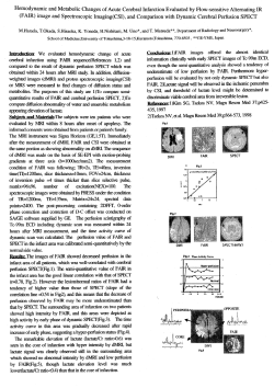


© Copyright 2026