1. home and garden
2. pest control

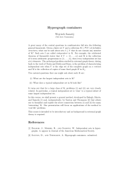
L1-minimization for mechanical systems
J.-B. Caillau∗
Z. Chen†
Y. Chitour‡
March 2015
Abstract
Second order systems whose drift is defined by the gradient of a given
potential are considered, and minimization of the L1 -norm of the control
is addressed. An analysis of the extremal flow emphasizes the role of singular trajectories of order two [25, 29]; the case of the two-body potential
is treated in detail. In L1 -minimization, regular extremals are associated
with controls whose norm is bang-bang; in order to assess their optimality
properties, sufficient conditions are given for broken extremals and related
to the no-fold conditions of [20]. An example of numerical verification of
these conditions is proposed on a problem coming from space mechanics.
Keywords. L1 -minimization, second order mechanical systems, order
two singular trajectories, no-fold conditions for broken extremals, twobody problem
MSC classification. 49K15, 70Q05
1
Introduction
This paper is concerned with the optimal control of mechanical systems of the
following form:
q¨(t) + ∇V (q(t)) =
u(t)
,
M (t)
M˙ (t) = −β|u(t)|,
where q is valued in an open subset Q of Rm , m ≥ 2, on which the potential
V is defined. The second equation describes the variation of the mass, M , of
the system when a control is used (β is some nonnegative constant). The finite
dimensional norm is Euclidean,
q
|u| = u21 + · · · + u2m
∗ Math. Institute, Univ. Bourgogne & CNRS/INRIA (jean-baptiste.caillau@u-bourgo
gne.fr). Part of this work was done during a sabbatical leave at Lab. J.-L. Lions, Univ. Paris
VI & CNRS, whose hospitality is gratefully acknowledged.
† Math. Dep., Univ. Paris-Sud & CNRS and Northwestern Polytechnical Univ.
([email protected]). Supported by Chinese Scholarship Council (grant no. 2013
0629 0024).
‡ L2S-Supelec, Univ. Paris-Sud & CNRS ([email protected]).
1
L1 -minimization for mechanical systems
2
and a constraint on the control is assumed,
|u(t)| ≤ ε,
ε > 0.
(1)
Given boundary conditions in the n-dimensional state (phase) space X := T Q '
Q × Rm (n = 2m), the problem of interest is the minimization of consumption,
that is the maximization of the final mass M (tf ) for a fixed final time. Clearly,
this amounts to minimizing the L1 -norm of the control,
Z tf
|u(t)| dt → min .
(2)
0
Up to some rescaling, there are actually two cases, β = 1 or β = 0. In the second
one, the mass is constant; though maximizing the final mass does not make sense
anymore, the Lagrange cost (2) is still meaningful. Actually, as propellant is
only a limited fraction of the total mass, one can expect this idealized constant
mass model to capture the main features of the original problem. We shall
henceforth assume β = 0, so the state reduces to x := (q, v) with v := q.
˙
In finite dimensions, `1 -minimization is well-known to generate sparse solutions having a lot of zero components; this fact translates here into the existence
of subintervals of time where the control vanishes, as is clear when applying the
maximum principle (see §2). This intuitively goes along well with the idea of
minimizing consumption: There are privileged values of the state where the
control is more efficient and should be switched on (burn arcs), while there are
some others where it should be switched off (cost arcs). (See also [5] for a different kind of interpretation in a biological setting, again with L1 -minimization.)
The resulting sparsity of the solution is then tuned by the ratio of the fixed final
time over the minimum time associated with the boundary conditions: While a
simple consequence of the form of the dynamics (and of the ball constraint on
the control) is that the min. time control norm is constant and maximum everywhere for the constant mass model,1 the extra amount of time available allows
for some optimization that results in the existence of subarcs of the trajectory
with zero control. (See Proposition 1, in this respect.) A salient peculiarity
of the infinite dimensional setting is the existence of subarcs with intermediate
value of the norm of the control, namely singular arcs. This was analyzed in
the seminal paper of Robbins [25] in the case of the two-body potential, providing yet another example of the fruitful exchanges between space mechanics and
optimal control in the early years of both disciplines. The consequence of these
singular arcs being of order two was further realized by Marchal who studied
chattering in [18]; this example comes probably second after the historical one
of Fuller [12] and has been thoroughly investigated by Zelikin and Borisov in
[29, 30].
A typical example of second order controlled system is the restricted threebody problem [8] where, in complex notation (R2 ' C),
Vµ (t, q) := −
µ
1−µ
−
·
it
|q + µe | |q − (1 − µ)eit |
In this case, µ is the ratio of the masses of the two primary celestial bodies, in
circular motion around their common center of mass. The controlled third body
1 See, e.g., [10]; this fact remains true for time minimization if the mass is varied provided
the mass at final time is left free [ibid].
L1 -minimization for mechanical systems
3
is a spacecraft gravitating in the potential generated by the two primaries, but
not influencing their motion. When µ = 0, the potential is autonomous and one
retrieves the standard controlled two-body problem. The study of ”continuous”
(as opposed to impulsive) strategies for the control began in the 60’s; see, e.g.,
the work of Lawden [16], or Beletsky’s book [3] where the importance of low
thrust (small ε in (1)) to spiral out from a given initial orbit was foreseen.
There is currently a strong interest for low-thrust missions with, e.g., the Lisa
Pathfinder [17] one of ESA2 towards the L1 Lagrange point of the Sun-Earth
system, or BepiColombo [4] mission of ESA and JAXA3 to Mercury.
An important issue in optimal control is the ability to verify sufficient optimality conditions. In L1 -minimization, the first candidates for optimality are
controls whose norm is bang-bang, switching from zero to the bound prescribed
by (1) (more complicated situations including singular controls). Second order
conditions in the bang-bang case have received quite an extensive treatment;
references include the paper of Sarychev [26], followed by [2] and [19, 22, 23].
On a similar line, the stronger notion of state optimality was introduced in [24]
for free final time. More recently, a regularization procedure has been developed
in [27] for single-input systems. These papers consider controls valued in polyhedra; the standing assumptions allow to define a finite dimensional accessory
optimization problem in the switching times only. Then, checking a second order sufficient condition on this auxiliary problem turns to be sufficient to ensure
strong local optimality of the bang-bang controls. A byproduct of the analysis is that conjugate times, where local optimality is lost, are switching times.
A different approach, based on Hamilton-Jacobi-Bellman and the method of
characteristics in optimal control, has been proposed by Noble and Sch¨attler
in [20]. Their results encompass the case of broken extremals with conjugate
points occuring at or between switching times. We provide a similar analysis
by requiring some generalized (with respect to the smooth case) disconjugacy
condition on the Jacobi fields, and using instead a Hamiltonian point of view
reminiscent of [11, 15]. Treating the case of such broken extremals is crucial
for L1 -minimization: As the finite dimensional norm of the control involved in
the constraint (1) and in the cost (2) is an `2 -norm, the control is valued in the
Euclidean ball of Rm , not a polyhedron if m > 1. When m = 1, the situation is
degenerate, and one can for instance set u = u+ − u− , with u+ , u− ≥ 0. (This
approach also works for m > 1 when an `1 or `∞ -norm is used for the values of
the control; see, e.g., [28].) When m > 1, it is clear using spherical coordinates
that although the norm of the control might be bang-bang, the variations of
the control component on Sm−1 preclude the reduction to a finite dimensional
optimization problem. (The same remark holds true for any `p -norm of the
control values with 1 < p < ∞.) An example of conjugacy occuring between
switching times is provided in §4.
The paper is organized as follows. In section 2, the extremal lifts of L1 minimizing trajectories are studied for an arbitrary potential in the constant
mass case; the properties of the flow are encoded by the Poisson structure defined by two Hamiltonians. In section 3, sufficient conditions for strong local
optimality of broken extremals with regular switching points are given in terms
of jumps on the Jacobi fields; these conditions are related to the no-fold con2 European
3 Japan
Space Agency.
Aerospace Exploration Agency.
L1 -minimization for mechanical systems
4
dition of [20]. In section 4 some numerical results illustrating the verification
of these sufficient conditions for L1 -minimizing trajectories are given. The twobody mechanical potential is considered, completing the study of Gergaud and
Haberkorn [13] where the first numerical computation of fuel minimizing controls with hundreds of switchings (for low thrust) was performed using a clever
combination of shooting and homotopy techniques. (See also [21] in the case of
a few switchings.) The classical construction of fields of extremals in the smooth
case is reviewed in an appendix.
2
Singularity analysis of the extremal flow
By renormalizing the time and the potential, one can assume ε = 1 in (1), so
we consider the L1 -minimum control of
q¨(t) + ∇V (q(t)) = u(t),
|u(t)| ≤ 1,
with x(t) = (q(t), v(t)) ∈ X = T Q (v(t) = q(t)),
˙
Q an open subset of Rm
(m ≥ 2), and make the following assumptions on the boundary conditions:
x(0) = x0
and x(tf ) ∈ Xf ⊂ X
where (i) x0 does not belong to the terminal submanifold Xf , (ii) Xf is invariant
wrt. the flow of the drift,4
F0 (q, v) = v
∂
∂
− ∇V (q)
,
∂q
∂v
and (iii) the fixed final time tf is supposed strictly greater than the minimum
time tf (x0 , Xf ) < ∞ of the problem. As the cost is not differentiable for u = 0,
rather than using a non-smooth maximum principle (compare, e.g., [5]) we make
a simple desingularization: In spherical coordinates, u = ρw where ρ ∈ [0, 1] and
w ∈ Sm−1 ; the change of coordinates amounts to adding an Sm−1 fiber above
the singularity u = 0 of the cost. In these coordinates, the dynamics write
x(t)
˙
= F0 (x(t)) + ρ(t)
m
X
wi (t)Fi (x(t))
i=1
with canonical Fi = ∂/∂vi , i = 1, . . . , m, and the criterion is linearized:
Z tf
ρ(t) dt → min .
0
The Hamiltonian of the problem is
H(x, p, ρ, w) = p0 ρ + H0 (x, p) + ρ
m
X
wi ψi (x, p)
i=1
where H0 (x, p) := pF0 (x) and the ψi (x, p) := pFi (x) are the Hamiltonian lifts
of the Fi , i = 1, . . . , m. Readily, H ≤ H0 + ρH1 with
v
um
uX
ψi2 ,
H1 := p0 + t
i=1
4 This assumption can be weakened; it is only used to ensure that a time minimizing control
extended by zero beyond the min. time is admissible. (See Lemma 1.)
L1 -minimization for mechanical systems
5
and the equality can always be achieved for some w ∈ Sm−1 : w = ψ/|ψ|
whenever ψ := (ψ1 , . . . , ψm ) is not zero, any w on the sphere otherwise. By
virtue of the maximum principle, if (ρ, w) is a measurable minimizing control
then the associated trajectory is the projection of an integral curve (x, p) :
[0, tf ] → T ∗ X of H0 + ρH1 such that, a.e.,
H0 (x(t), p(t)) + ρ(t)H1 (x(t), p(t)) = max H0 (x(t), p(t)) + rH1 (x(t), p(t)). (3)
r∈[0,1]
Moreover, the constant p0 is nonpositive and (p0 , p) 6= (0, 0). Either p0 = 0
(abnormal case), or p0 can be set to −1 by homogeneity (normal case).
Proposition 1 (Gergaud et al. [13]). There are no abnormal extremals.
Lemma 1. The function ψ evaluated along an extremal has only isolated zeros.
Proof. As a function of time when evaluated along an extremal, ψ is absolutely
continous and, a.e. on [0, tf ],
ψ˙ i (t) = p(t)[F0 , Fi ](x(t)),
i = 1, . . . , m.
˙
As a result, ψ is a C 1 function of time and, if ψ(t) = 0, then ψ(t)
6= 0; indeed,
the rank of {F1 , . . . , Fm , [F0 , F1 ], . . . , [F0 , Fm ]} is maximum everywhere, so p(t)
would otherwise be zero. Since p is solution of a linear ode, this would imply that
it vanishes identically; necessarily p0 < 0, so ρ would also be zero a.e. because
of the maximization condition (3). This is impossible because x0 ∈
/ Xf .
Proof of the Proposition. By contradiction: Assume p0 = 0; as ψ has only isolated zeros according to the previous lemma, ρ = 1 a.e. by maximization. The
resulting cost is equal to tf . Now, the target submanifold Xf is invariant by the
drift, so any minimizing control extended by u = 0 on [tf , tf ] (where tf denotes
the min. time) remains admissible. It has a cost equal to tf < tf , hence the
contradiction.
We set p0 = −1, so H1 = |ψ| − 1. In contrast with the minimum time case,
the singularity ψ = 0 does not play any role in L1 -minimization. In the neighbourhood of t such that ψ(t) = 0, H1 is negative, so ρ = 0. Locally, the control
vanishes and the extremal is smooth. The only effect of the singularity is a
discontinuity in the Sm−1 fiber over u = 0 in which w(t+) = −w(t−) (see [10]).
The important remaining singularity is H1 = 0. As opposed to the standard
single-input case, H1 is not the lift of a vector field on X; the properties of the
extremal flow depend on H0 , H1 , and their Poisson brackets. (See also §4 for
the consequences in terms of second order conditions.) We denote by H01 the
bracket {H0 , H1 }, and so forth. The following result is standard (see [6], e.g.)
and accounts for the intertwining of arcs along which ρ = 0 (labeled γ0 ) with
arcs such that ρ = 1 (labeled γ+ ).
Proposition 2. In the neighbourhood of z0 in {H1 = 0} such that H01 (z0 ) 6= 0,
every extremal is locally bang-bang of the form γ0 γ+ or γ+ γ0 , depending on the
sign of H01 (z0 ).
L1 -minimization for mechanical systems
6
Proof. As H01 (z0 ) 6= 0, H1 must be a submersion at z0 , so {H1 = 0} is locally
a codimension one submanifold splitting T ∗ X into {H1 < 0} and {H1 > 0}.
Evaluated along an extremal, H1 is a C 1 function of time since
H˙ 1 (t) = {H0 + ρ(t)H1 , H1 } = H01 (t).
Through z0 passes only one extremal, and it is of the form γ0 γ+ if H01 (z0 ) > 0
(resp. γ+ γ0 if H01 (z0 ) < 0). The bracket condition allows to use the implicit
function theorem to prove that neighbouring extremals also cross {H1 = 0}
transversally.
Such switching points are termed regular and are studied in §3 from the point
of view of second order optimality conditions. Besides the occurence of γ0 arcs
resulting in the parsimony of solutions as explained in the introduction, the
peculiarity of the control setting is the existence of singular arcs along which
H1 vanishes identically. On such arcs, ρ may take arbitrary values in [0, 1].
Theorem 1 (Robbins [25]). Singular extremals are at least of order two, and
minimizing singulars of order two are contained in
{z = (q, v, pq , pv ) ∈ T ∗ X | V 00 (q)p2v ≥ 0, V 000 (q)p3v > 0}.
Proof. One has H0 = (pq |v) − (pv |∇V (q)), and H1 = 0 along a singular so,
0 = H01 = −
1
(pq |pv )
|pv |
along the arc.
Lemma 2. On T ∗ X, H101 = H1001 = 0.
Proof. Computing,
H101 = {H1 , H01 } = {|pv | − 1, −
1
(pq |pv )} = 0,
|pv |
and it is standard that
H1001
= {H1 , {H0 , H01 }}
= {−H01 , H01 } + {H0 , H101 }
= 0
using Leibniz rule.
Then 0 = H˙ 01 = H001 + ρH101 implies H001 = 0 along a singular arc. Iterating,
0 = H˙ 001 = H0001 + ρH1001 so, by the previous lemma again, 0 = H0001 .
Eventually, 0 = H˙ 0001 = H00001 +ρH10001 . Set f := H0 , g := H1 , h := −(pq |pv ),
so that H01 = βh with β = 1/|pv |. Using Leibniz rule, the following is clear.
Lemma 3.
(adk f )(βh)|(adi f )h=0,
0≤i<k
= β(adk f )h
{g, (adk f )(βh)}|(adi f )h=0,
0≤i≤k
= β{g, (adk f )h}
L1 -minimization for mechanical systems
7
Computing, one obtains
(adf )h = −V 00 (q)p2v + |pq |2 ,
so 0 = H001 implies V 00 (q)p2v ≥ 0, and
(ad2 f )h = −V 000 (q)(v, pv , pv ) + 4V 00 (q)(pq , pv ),
{g, (ad2 f )h} = −
1 000
V (q)p3v .
|pv |
Through a point z0 such that the last quantity does not vanish, there passes a
so-called order two singular extremal that is an integral curve of the Hamiltonian
Hs := H0 + ρs H1 with the dynamic feedback
ρs := −
H00001
·
H10001
Along such a minimizing singular arc, the generalized Legrendre condition must
hold, H10001 ≤ 0, so V 000 (q)p3v > 0.
Corollary 1. In the case of the two-body potential V (q) = −1/|q| (q 6= 0), along
an order two singular arc one has either α ∈ (π/2, α0 ] or α ∈ [−α0 , −π/2)
√where
α is the angle of the control with the radial direction, and α0 = acos(1/ 3).
Proof. One has
V 0 (q)pv =
(pv |q)
,
|q|3
V 000 (q)p3v = −
V 00 (q)p2v =
|pv |2
3(pv |q)2
−
,
3
|q|
|q|5
9(pv |q)|pv |2
15(pv |q)3
+
·
5
|q|
|q|7
On Q = Rm \{0}, Sm−1 3 w = pv since |pv | = 1 along a singular arc, so
cos α = (pv |q)/|q|. The condition V 00 (q)p2v ≥ 0 reads 1 − 3 cos2 α ≥ 0, and
V 000 (q)p3v > 0 is fulfilled if and only if
cos α(3 − 5 cos2 α) < 0
that is provided cos α < 0 in addition to the previous condition. Hence the two
cases (in exclusion since the singular control is smooth) for the angle.
The existence of order two singular arcs in the two-body case results in the
well-known Fuller or chattering phenomenon [18, 29]. The same phenomenon
actually persists for the restricted three body problem as is explained in [30].
Altough these singular trajectories are contained in some submanifold of the
cotangent space with codimension > 1, their existence rules out the possibility to bound globally the number of switchings of regular extremals described
by Proposition 2. The next section is devoted to giving sufficient optimality
conditions for such bang-bang extremals.
L1 -minimization for mechanical systems
3
8
Sufficient conditions for extremals with regular switchings
Let X be an open subset of Rn , U a nonempty subset of Rm , f a vector field
on X parameterized by u ∈ U , and f 0 : X × U → R a cost function, all smooth.
Consider the following minimization problem with fixed final time tf : Find
(x, u) : [0, tf ] → X × U , x absolutely continous, u measurable and bounded,
such that
x(t)
˙
= f (x(t), u(t)), t ∈ [0, tf ] (a.e),
x(0) = x0 ,
and such that
Z
x(tf ) = xf ,
tf
f 0 (x(t), u(t)) dt
0
is minimized. The maximum principle asserts that, if (x, u) is such a pair, there
exists an absolutely continuous lift (x, p) : [0, tf ] → T ∗ X and a nonpositive
scalar p0 , (p0 , p) 6= (0, 0), such that a.e. on [0, tf ]
∂H
˙
x(t)
=
(x(t), p(t), u(t)) ,
∂p
∂H
˙
p(t)
=−
(x(t), p(t), u(t)) ,
∂x
and
H(x(t), p(t), u(t)) = max H(x(t), p(t), ·)
U
∗
where H : T X × U → R is the Hamiltonian of the problem,
H(x, p, u) := p0 f 0 (x, u) + pf (x, u).
We first assume that
(A0) The reference extremal is normal.
Accordingly, p0 can be set to −1. Let H1 , H2 : T ∗ X → R be two smooth
functions, and denote Σ := {H1 = H2 }, Ω1 := {H1 > H2 } (Ω2 := {H2 > H1 },
resp.) We assume that
max H(z, ·) = Hi ,
U
z ∈ Ωi ,
i = 1, 2,
(4)
and follow the point of view of [11] that these two Hamiltonians are competing
Hamiltonians. Let (x, p, u) be a reference extremal having only one contact
with Σ at z 1 := z(t1 ), t1 ∈ (0, tf ) (z := (x, p)). We denote H12 = {H1 , H2 } the
Poisson bracket of H1 with H2 and make the following assumption:
(A1) H12 (z 1 ) > 0.
In [15] terms, z 1 is a regular (or normal ) switching point. This condition is
called the strict bang-bang Legendre condition in [2]. The analysis of this section
readily extends to a finite number of such switchings.
Lemma 4. z is the concatenation of the flows of H1 and then H2 .
L1 -minimization for mechanical systems
9
Proof. The extremal having only one contact with Σ at z 1 , z(t) is either in Ω1
or Ω2 for t 6= t1 . Because of (4), the maximization condition of the maximum
principle implies that z is given by the flow of either H1 or H2 on [0, t1 ]. In
both cases,
d
(H1 − H2 )(z(t))|t=t1 = −H12 (z 1 ) < 0,
dt
so H1 > H2 before t1 (H2 > H1 after t1 , resp.) and the only possibility is an
H1 then H2 concatenation of flows.
As a result of (A1), Σ is a codimension one submanifold in the nbd of z 1 , and
one can define locally a function z0 7→ t1 (z0 ) such that z1 (t1 (z0 ), z0 ) belongs to
Σ for z0 in a nbd of z 0 := z(0). As we have just done, we will denote
→
−
zi (t, z0 ) = et H i (z0 ),
i = 1, 2,
the Hamiltonian flows of H1 and H2 . These flows will be assumed complete for
the sake of simplicity. We will denote 0 = ∂/∂z for flows. Clearly,
Lemma 5.
t01 (z0 ) =
(H1 − H2 )0
(z1 (t1 (z0 ), z0 ))z10 (t1 (z0 ), z0 ).
H12
One then defines locally z0 7→ z(t, z0 ) = (x(t, z0 ), p(t, z0 )) := z1 (t, z0 ) if t ≤
t1 (z0 ), and z(t, z0 ) := z2 (t − t1 (z0 ), z1 (t1 (z0 ), z0 )) if t ≥ t1 (z0 ). We recall the
following standard computation:
Lemma 6. For t > t1 (z0 ),
∂z
(t, z0 ) = z20 (t − t1 (z0 ), z1 (t1 (z0 ), z0 ))(I + σ(z0 ))z10 (t1 (z0 ), z0 )
∂z0
with
−−−−−−→ (H1 − H2 )0
σ(z0 ) = H1 − H2
(z1 (t1 (z0 ), z0 )).
H12
(5)
Proof. The derivative is equal to (arguments omitted)
−z˙2 t01 + z20 (z˙1 t01 + z10 ),
hence the result by factoring out z20 and using Lemma 5 plus the fact that the
adjoint action of a flow is idempotent on its generator,
→
−
→
−
(z20 (s, z))−1 H 2 (z2 (s, z)) = H 2 (z),
The function
δ(t) := det
∂x
(t, z 0 ),
∂p0
(s, z) ∈ R × T ∗ X.
t 6= t1 ,
(6)
is piecewise continuous along the reference extremal, and we make the additional
assumption that
(A2) δ(t) 6= 0, t ∈ (0, t1 ) ∪ (t1 , tf ], and δ(t1 +)δ(t1 −) > 0.
L1 -minimization for mechanical systems
10
This condition means that we assume disconjugacy on (0, t1 ] and [t1 , tf ] along
the linearized flows of H1 and H2 , respectively, and that the jump (encoded by
the matrix σ(z0 )) in the Jacobi fields is such that there is no sign change in the
determinant. This is exactly the condition one is able to check numerically by
computing Jacobi fields (see [6, 7], e.g.). As will be clear from the proof of the
result below, geometrically this assumption is the no-fold condition of [20] (no
fold outside t1 , no broken fold at t1 ).
Theorem 2. Under assumptions (A0)-(A2), the reference trajectory is a C 0 local minimizer among all trajectories with same endpoints.
Proof. We proceed in five steps.
Step 1. According to (A2), ∂x1 /∂p0 (t, z 0 ) is invertible for t ∈ (0, t1 ]; one can
then construct a Lagrangian perturbation L0 transverse to Tx∗0 X containing
z 0 such that ∂x1 /∂z0 (t, z 0 ) is invertible for t ∈ [0, t1 ], t = 0 included, ∂/∂z0
denoting the n partials wrt. z0 ∈ L0 . (See appendix A.) For ε > 0 small enough
define
L1 := {(t, z) ∈ R × T ∗ X | (∃z0 ∈ L0 ) : t ∈ (−ε, t1 (z0 ) + ε) s.t. z = z1 (t, z0 )}.
By restricting L0 if necessary, Π : R × T ∗ X → R × X, (t, z) 7→ (t, x) induces a
diffeomorphism of L1 onto its image. Similarly, (A2) implies that
∂
[x2 (t − t1 (z0 ), z1 (t1 (z0 ), z0 ))] |z0 =z0
∂p0
is invertible for t ∈ [t1 , tf ]; restricting again L0 if necessary, one can assume
that Π also induces a diffeomorphism from
L2 := {(t, z) ∈ R × T ∗ X | (∃z0 ∈ L0 ) : t ∈ (t1 (z0 ) − ε, tf + ε)
s.t. z = z2 (t − t1 (z0 ), z1 (t1 (z0 ), z0 ))}
onto its image.
Step 2. Define Σ1 := L1 ∩(R×Σ). As (t, z0 ) 7→ (t, x1 (t, z0 )) is a diffeomorphism
from R × L0 onto Π(L1 ), there exists an inverse function z0 (t, x) such that
Π(Σ1 ) = {ψ = 0} with
ψ(t, x) := t − t1 (z0 (t, x)).
Denote ψ(t) := ψ(t, x(t)) the evaluation of this function along the reference
˙ 1 −) = 1 > 0 and (compare [20])
trajectory. By construction, ψ(t
˙ 1 +) = 1 + ∂t1 (z 0 )
ψ(t
∂z0
−1
∂x1
(t1 , z 0 )
∇p (H1 − H2 )(z 1 ).
∂z0
Lemma 7.
∂t1
δ(t1 +) = δ(t1 −) 1 +
(z 0 )
∂p0
!
−1
∂x1
(t1 , z 0 )
∇p (H1 − H2 )(z 1 ) .
∂p0
(7)
L1 -minimization for mechanical systems
11
Proof. By virtue of Lemma 6,
∂x
∂x1
(H1 − H2 )0
∂z1
(t1 +, z 0 ) =
(t1 , z 0 ) + ∇p (H1 − H2 )
(z 1 )
(t1 , z 0 )
∂p0
∂p0
H12
∂p0
|
{z
}
∂t1
=
(z 0 )
∂p0
(the second equality coming from Lemma 5). Assumption (A2) implies δ(t1 −) 6=
0 so, taking determinants,
!
−1
∂x1
∂t1
∇p (H1 − H2 )(z 1 )
δ(t1 +) = δ(t1 −) det I +
(t1 , z 0 )
(z 0 )
∂p0
∂p0
!
−1
∂t1
∂x1
= δ(t1 −) 1 +
(z 0 )
(t1 , z 0 )
∇p (H1 − H2 )(z 1 )
∂p0
∂p0
as det(I + x t y) = 1 + (x|y).
Since δ(t1 +) and δ(t1 −) have the same sign, the quantity in brackets in (7)
˙ 1 +) > 0 as L0 can be taken arbitrarily close
must be positive. Accordingly, ψ(t
∗
to Tx0 X. So, locally, Π(Σ1 ) is a submanifold that splits R × X in two and, by
restricting L0 if necessary, every extremal of the field t 7→ x(t, z0 ) for z0 ∈ L0
crosses Π(Σ1 ) transversally. Defining
L1− := {(t, z) ∈ R × T ∗ X | (∃z0 ∈ L0 ) : t ∈ [0, t1 (z0 )] s.t. z = z1 (t, z0 )}
and
L2+ := {(t, z) ∈ R × T ∗ X | (∃z0 ∈ L0 ) : t ∈ [t1 (z0 ), tf ]
s.t. z = z2 (t − t1 (z0 ), z1 (t1 (z0 ), z0 ))},
one can hence piece together the restrictions of Π to L1− and L2+ into a continuous bijection from L1− ∪ L2+ into Π(L1− ∪ L2+ ). By restricting to a compact
neighbourhood of the graph of z, one may assume that Π induces a homeomorphism on its image.
Step 3. Denote αi := p dx − Hi (z)dt, i = 1, 2, the Poincar´e-Cartan forms
associated with H1 and H2 , respectively. To prove that α1 is exact on L1 , it
is enough to prove that it is closed. Indeed, if γ(s) := (t(s), z1 (t(s), z0 (s))) is
a closed curve on L1 , it retracts continuously on γ0 (s) := (0, z0 (s)) so that,
provided α1 is closed,
Z
Z
Z
α1 =
α1 =
p dx = 0
γ
γ0
γ0
because z0 (s) belongs to L0 that can be chosen such that p dx is exact on it.
(Compare [1, §17].) Similarly, to prove that α2 is exact on L2 , it suffices to
prove that it is closed: If γ(s) := (t(s), z2 (t(s) − t1 (z0 (s)), z1 (t1 (z0 (s)), z0 (s))))
is a closed curve in L2 , it readily retracts continuously on the curve γ1 (s) :=
(t1 (z0 (s)), z1 (t1 (z0 (s)), z0 (s))) in Σ1 , which retracts continuously on γ0 (s) :=
(0, z0 (s)) again. Then, as H1 = H2 on Σ,
Z
Z
Z
Z
α2 =
α2 =
α1 =
α1
γ
γ1
γ1
γ0
L1 -minimization for mechanical systems
12
Figure 1: The field of extremals.
that vanishes as before. To prove that α1 is closed, consider tangent vectors at
(t, z) ∈ L1 ; a parameterization of this tangent space is
→
−
(δt, H 1 (z)δt + z10 (t, z0 )δz0 ),
(δt, δz0 ) ∈ R × Tz0 L0
where z0 ∈ L0 is such that z = z1 (t, z0 ). For two such vectors v1 , v2 ,
dα1 (t, z)(v1 , v2 )
= (dp ∧ dx − dH1 (z)dt)(v1 , v2 )
= dp ∧ dx(z10 (t, z0 )δz01 , z10 (t, z0 )δz02 )
= dp ∧ dx(δz01 , δz02 )
= 0
L1 -minimization for mechanical systems
13
→
−
because exp(t H 1 ) is symplectic and L0 is Lagrangian. Regarding α2 , the tangent space at (t, z) ∈ L2 is parameterized according to
→
−
(δt, H 2 (z)δt + z20 (t − t1 (z0 ), z1 (t1 (z0 ), z0 ))(I + σ(z0 ))z10 (t, z0 )δz0 )
with (δt, δz0 ) ∈ R × Tz0 L0 , and where z0 ∈ L0 is such that z = z2 (t −
t1 (z0 ), z1 (t1 (z0 ), z0 )). For two such vectors v1 , v2 ,
dα2 (t, z)(v1 , v2 )
= (dp ∧ dx − dH2 (z)dt)(v1 , v2 )
= dp ∧ dx((I + σ(z0 ))z10 (t, z0 )δz01 , (I + σ(z0 ))z10 (t, z0 )δz02 )
= dp ∧ dx(z10 (t, z0 )δz01 , z10 (t, z0 )δz02 )
→
−
because exp(t H 2 ) is symplectic and because
Lemma 8.
I + σ(z0 ) ∈ Sp(2n, R).
Proof. For any z ∈ R2n ,
t
t
(I + Jz t z)J(I + Jz t z) = J − z t z + z t z + z(|t zJz
{z }) z = J.
0
This proves the lemma because of the definition (5) of σ(z0 ).
→
−
One then concludes as before that α2 is closed using the fact that exp(t H 1 ) is
symplectic and L0 is Lagrangian.
Step 4. Let (x, u) : [0, tf ] → X × U be an admissible pair. We first assume that
x is of class C 1 and that its graph has only one isolated contact with Π(Σ1 ),
at some point point (t1 , x(t1 )). For x close enough to x in the C 0 -topology,
this graph has a unique lift t 7→ (t, x(t), p(t)) in L1− ∪ L2+ . As a gluing at t1
of two absolutely continous functions, z := (x, p) : [0, tf ] → T ∗ X is absolutely
continous. Denote γ1 and γ2 the two pieces of this lift. Denote similarly γ 1 and
γ 2 the pieces of the graph of the extremal z (see Fig. 2). One has
Z t1 Z tf Z tf
0
f (x(t), u(t)) dt =
+
(p(t)x(t)
˙ − H(x(t), p(t), u(t))) dt
0
Z
0
t1
≥
t1
(p(t)x(t)
˙ − H1 (x(t), p(t))) dt
0
Z
tf
+
t1
Z
=
γ1
(p(t)x(t)
˙ − H2 (x(t), p(t))) dt
Z
α1 +
α2
γ2
since z(t) belongs to Ω1 for t ∈ [0, t1 ) (resp. to Ω2 for t ∈ (t1 , tf ]). By connectedness, there exists a smooth curve γ12 ⊂ Σ1 connecting (t1 , z(t1 )) to (t1 , z(t1 ));
L1 -minimization for mechanical systems
14
Figure 2: Integration paths.
having the same endpoints, γ1 and γ 1 ∪ γ12 (resp. γ2 and −γ12 ∪ γ 2 ) are homotopic. Since α1 and α2 are exact one forms on L1 and L2 , respectively,
Z
Z
Z
Z
α1 +
α2 =
α1 +
α2
γ1
γ2
γ ∪γ
−γ12 ∪γ 2
Z 1 12 Z
=
α1 +
α2
γ1
tf
Z
γ2
f 0 (x(t), u(t)) dt
=
0
since H1 = H2 on Σ.
Step 5. Consider finally an admissible pair (x, u), x close enough to x in the
C 0 -topology. One can find x
e of class C 1 arbitrarily close to x in the W1,∞ topology such that x
e(0) = x0 and x
e(tf ) = xf . Moreover, as Π(Σ1 ) is a locally
a smooth manifold, up to some C 1 -small perturbation one can assume that the
graph of x
e has only transverse intersections with Π(Σ1 ). Let ze := (e
x, pe) denote
the associated lift; one has
f 0 (e
x(t), u(t)) = (e
p(t)x
e˙ (t) − H(e
x(t), pe(t), u(t))) + pe(t)(f (e
x(t), u(t)) − x
e˙ (t)),
and the second term in the right-hand side can be made arbitrarily small when
x
e gets closer to x in the W1,∞ -topology since (t, ze(t)) = Π−1 (t, x
e(t)) remains
bounded by continuity of the inverse of Π. Let then ε > 0; as a result of the
previous discussion, there exists x
e of class C 1 with same endpoints as x and
whose graph has only isolated contacts with Π(Σ1 ) such that
Z tf
Z tf
0
f (x(t), u(t)) dt ≥
f 0 (e
x(t), u(t)) dt − ε,
0
0
L1 -minimization for mechanical systems
Z
tf
0
Z
f (e
x(t), u(t)) dt ≥
0
0
tf
15
(e
p(t)x
e˙ (t) − H(e
x(t), pe(t), u(t))) dt − ε.
One can extend straightforwardly the analysis of the previous step to finitely
many contacts with Π(Σ1 ), and bound below the integral in the right-hand side
of the second inequality by the cost of the reference trajectory. As ε is arbitrary,
this allows to conclude.
4
Numerical example: The two-body potential
Following [13], we consider the two-body controlled problem in dimension three.
Restricting to negative energy, orbits of the uncontrolled motion are ellipses,
and the issue is to realize minimum fuel transfer between non-coplanar orbits
around a fixed center of mass. The potential is V (q) := −µ/|q| defined on
Q := {q ∈ R3 | q 6= 0}, and we actually restrict to
X := {(q, v) ∈ T Q | |v|2 /2 − µ/|q| < 0, q ∧ v > 0}.
(The last condition on the momentum avoids collisional trajectories and orientates the elliptic orbits.) The constant µ is the gravitational constant that
depends on the attracting celestial body. To keep things clear, a medium thrust
case is presented below; the final time is fixed to 1.3 times the minimum time,
approximately, which already ensures a satisfying gain of consumption [13]. In
order to have fixed endpoints to perform a conjugate point test according to §3
result, initial and final positions are fixed on the orbits (fixed longitudes5 ). A
more relevant treatment would leave the final longitude free (in accordance with
assumption (ii) on the target in §2); this would require a focal point test that
could be done much in the same way (see, e.g., [9]). See Tab. 1 for a summary
of the physical constants.
As explained in §2, the L1 -minimization results in a competition between
two Hamiltonians: H0 (coming from the drift, only), and H0 + H1 (assuming
the control bound is normalized to 1 after some rescaling). Both Hamiltonians
are smooth and fit in the framework set up in §3 to check sufficient optimality
conditions. Restricting to bang-bang (in the norm of the control) extremals,
regularity of the switchings is easily verified numerically, while normality is
taken care of by Proposition 1. Then one has to check the no-fold condition on
the Jacobi fields. The optimal solution (see Fig. 3) and these fields are computed
using the hampath software [14]; as in [9, 13], a regularization by homotopy is
used to capture the switching structure and initialize the computation of the
bang-bang extremal by single shooting. We are then able to check condition
(A2) directly on this extremal by a simple sign test (including the jumps on
the Jacobi fields at the regular switchings) on the determinant of the fields (see
Fig. 4). An alternative approach would be to establish a convergence result as
in [27], and to verify the second order conditions on the sequence of regularized
extremals. As underlined in §1 and §3, conjugate times may occur at or between
5 Precisely, the longitude l is defined as the sum of three broken angles: l = Ω + θ + $,
where Ω is the longitude of the ascending node (first Euler angle of the orbit plane with the
equatorial plane; the second Euler angle defines the inclination of the orbit), θ is the argument
of perigee (angle of the semi-major axis of the ellipse, equal to the third Euler angle of the
orbit plane), and $ is the true anomaly (polar angle with respect to the semi-major axis in
the orbit plane). Here, Ω = θ = 0 on the initial and final orbits.
L1 -minimization for mechanical systems
16
Table 1: Summary of physical constants used for the numerical commputation.
398600.47 Km3 s−2
Gravitational constant µ of the Earth:
Mass of the spacecraft:
Initial
Initial
Initial
Initial
perigee:
apogee:
inclination:
longitude:
Minimum time:
1500 Kg
6643 Km
46500 Km
0.1222 rad
π rad
110.41 hours
Thrust:
Final
Final
Final
Final
10 Newtons
perigee:
apogee:
inclination:
longitude:
42165 Km
42165 Km
0 rad
56.659 rad
Fixed final time:
147.28 hours
L1 cost achieved (normalized):
67.617
switching times. On the example treated, no conjugate point is detected on
[0, tf ], ensuring strong local optimality. The extremal is then extended up to
3.5 tf , and a conjugate point is detected about 3.2 tf , at a switching point (sign
change occurint at the jump). A second test is provided Fig. 5; by perturbing
slightly the endpoint conditions, one observes that conjugacy occurs not at a
switching anymore, but along a burn arc.
Remark 1. As H0 is the lift of a vector field, the determinant of Jacobi fields
is either identically zero or non-vanishing along a cost arc (ρ = 0). (Compare
with the case of polyhedral control set; see also Corollary 3.9 in [20].) Moreover,
coming from a mechanical system, the drift F0 is the symplectic gradient of the
energy function,
1
E(q, v) := |v|2 + V (q).
2
Accordingly, the δx = (δq, δv) part of the Jacobi field (see appendix) along an
→
−
integral arc of H 0 verifies
→
−
δ x(t)
˙
= E 0 (x(t))δx(t),
so δx has a constant determinant along such an arc since the associated flow
is symplectic. In particular, the disconjugacy condition (A2) implies that the
optimal solution starts with a burn arc.
Conclusion
We have reviewed some of the particularities of L1 -minimization in the control
setting. Among these, the existence of singular controls valued in the interior
of the Euclidean ball comes in strong contrast with the finite dimensional case.
Moreover, these singular extremals are at least of order two, entailing existence
of chattering [29]. By changing coordinates on the control, one can reduce the
system to a single control, namely the norm of the original one. This emphasizes
the role played by the Poisson structure of two Hamiltonians, the second not the
lift of a vector field; this fact accounts for the possibility of conjugacy happening
L1 -minimization for mechanical systems
17
Figure 3: L1 minimum trajectory. The graph displays the trajectory (blue line),
as well as the action of the control (red arrows). The initial orbit is strongly
eccentric (0.75) and slightly inclined (7 degrees). The geostationary target orbit
around the Earth is reached at tf ' 147.28 hours. The sparse structure of the
control is clearly observed, with burn arcs concentrated around perigees and
apogees (see [13]). The minimization leads to thrust only 46% of the time.
not necessarily at switching times, as opposed to the simpler case of bang-bang
controls valued in polyhedra. Sufficient conditions for this type of extremals
have been given; they rely on a simple and numerically verifiable check on the
discontinuous Jacobi fields of the system. They are essentially equivalent to the
no-fold conditions of [20], formulated here in a Hamiltonian setting. The example of L1 -minimization for the three-dimensional two-body potential illustrates
the interest of the approach. Future work include the treatment of mass varying
systems (that is of maximization of the final mass) for more general problems
such as the restricted three-body one.
A
Sufficient conditions in the smooth case
Consider the same minimization problem as in §3. Suppose that
(B0) The reference extremal is normal.
Having fixed p0 to −1, we make the stronger assumption that the maximized
Hamiltonian is well defined and smooth, and set
h(z) := max H(z, ·),
U
z ∈ T ∗ X.
Scholium. For almost all t ∈ [0, tf ],
h0 (z(t)) =
∂H
(z(t), u(t)),
∂z
∇2 h(z(t)) − ∇2zz H(z(t), u(t)) ≥ 0.
Proof. For a.a. t ∈ [0, tf ], h(z(t)) − H(z(t), u(t)) = 0, while
h(z) − H(z, u(t)) ≥ 0,
z ∈ T ∗ X,
by definition of h. Applying the first and second order necessary conditions for
optimality on T ∗ X at z = z(t) gives the result.
L1 -minimization for mechanical systems
2
18
#10 -8
#10 -13
1.5
1
0
0.5
0
-2
-0.5
-1
-4
0
100
200
300
400
500
475
476
477
478
1
0.8
0.6
0.4
0.2
0
0
50
100
150
200
250
300
350
400
450
500
Figure 4: Conjugate point test on the bang-bang L1 -extremal extended to
[0, 3.5 tf ]. The value of the determinant of Jacobi fields (6) along the extremal
is plotted against time on the upper left subgraph. The first conjugate point
occurs at t1c ' 475.93 hours > tf ; optimality of the reference extremal on [0, tf ]
follows. On the upper right subgraph, a zoom is provided to show the jumps on
the Jacobi fields (then on their determinant) around the first conjugate time;
several jumps are observed, the first one leading to a sign change at the conjugate time. Note that in accordance with Remark 1, the determinant must
be constant along the cost arcs (ρ = 0) provided the symplectic coordinates
x = (q, v) are used; this is not the case here as the so called equinoctial elements [10] are used for the state—hence the slight change in the determinant.
The bang-bang norm of the control, rescaled to belong to [0, 1] and extended to
3.5 tf , is portrayed on the lower graph. On the extended time span, there are
already more than 70 switchings though the thrust is just a medium one. For
low thrusts, hundreds of switchings occur.
We make the following assumption on the smooth reference extremal.
(B1) ∂x/∂p0 (t, z 0 ) is invertible for t ∈ (0, tf ].
Theorem 3. Under assumptions (B0)-(B1), the reference trajectory is a C 0 local minimizer among all trajectories with same endpoints.
L1 -minimization for mechanical systems
1
19
#10 -8
#10 -14
2.5
0.5
2
0
1.5
-0.5
1
-1
0.5
-1.5
0
-2
-0.5
-2.5
-1
-3
-1.5
-3.5
-2
0
200
400
489
490
491
Figure 5: Conjugate point test on a perturbed bang-bang L1 -extremal extended
to [0, 3.5 tf ]. The value of the determinant of Jacobi fields (6) along the extremal
is plotted against time (detail on the right subgraph). The endpoint conditions
x0 , xf given in Tab. 1 are perturbed according to x ← x + ∆x, |∆x| ' 1e − 5,
leading to conjugacy not at but between switching points—along a burn arc
(ρ = 1). The first conjugate point occurs at t1c ' 489.23 hours > tf , ensuring
again optimality of the reference extremal on [0, tf ].
Note that no Legendre type assumption is made, and that the disconjugacy condition (B1) can be numerically verified (e.g., by a rank test while integrating the
variational system along the reference extremal). For the sake of completeness,
we provide a proof that essentially goes along the lines of [1, §21].
Proof. For S0 symmetric of order n, L0 := {δx0 = S0 δp0 } is a Lagrangian
subspace of Tz0 (T ∗ X). Denote by δz = (δx, δp) the solution of the linearized
system
→
−
δ z(t)
˙ = h 0 (z(t))δz(t), δz(0) = (S0 , I),
and set δe
z (t) = (δe
x(t), δe
p(t)) := Φ−1
t δz(t) where Φt is the fundamental solution
of the linearized system
→
−
∂H
˙
Φt =
(z(t), u(t))Φt ,
∂z
Φ0 = I.
As δp(0) = δe
p(0) = I,
S(t) := δe
x(t)δe
p(t)−1
is well defined for small enough t ≥ 0. Since
→
−
Lt := exp(t h )0 (z(t))(L0 )
and
Φ−1
t (Lt )
are Lagrangian as images of L0 through linear symplectic mappings, S(t) must
be symmetric.
˙
Lemma 9. S(t)
≥0
L1 -minimization for mechanical systems
20
Proof. Let t1 ≥ 0 such that S(t1 ) is well defined, and let ξ ∈ Rn . Set
ξ0 := δe
p(t1 )−1 ξ
and δe
z1 (t) := δe
z (t)ξ0 .
Then δe
z1 (t1 ) = (S(t1 )ξ, ξ), and δe
x1 (t) = S(t)δe
p1 (t). Differentiating the previous
relation and using S(t) symmetry leads to
˙
(S(t)δe
p1 (t)|δe
p1 (t)) = ω(δe
z1 (t), δ ze˙ 1 (t)).
Differentiating now
δe
z1 (t) = Φ−1
t δz(t)ξ0 ,
one gets
→
−
→0
−
∂H
−
(z(t), u(t)))Φt δe
z1 (t)
δ ze˙ 1 (t) = Φ−1
(
h
(z(t))
t
∂z
= J t Φt (∇2 h(z(t)) − ∇2zz H(z(t), u(t)))Φt δe
z1 (t).
|
{z
}
≥0
(J denotes the standard symplectic matrix.) Evaluating at t = t1 , one eventually
˙ 1 )ξ|ξ) ≥ 0.
gets (S(t
For S0 = 0, there is η > 0 such that S(t) is well defined on [0, η], which remains
true for S0 > 0, |S0 | small enough. By the lemma before, St > 0 on [0, η]. In
particular, it is an invertible matrix, which ensures that Φ−1
t (Lt ) is transversal
to ker π 0 (z 0 ) (π : T ∗ X → X being the canonical projection), that is Lt is
transversal to ker π 0 (z(t)) by virtue of
Scholium. Φt (ker π 0 (z 0 )) = ker π 0 (z(t))
Proof. Note that in the linearized system defining Φt ,
δ x(t)
˙
= ∇2xp H(z(t), u(t))δx(t),
δ p(t)
˙
= −∇2xx H(z(t), u(t))δx(t) − ∇2px H(z(t), u(t))δp(t),
the equation on δx is linear. Hence δx(0) = 0 implies δx ≡ 0.
By restricting if necessary |S0 |, (B1) allows to assume that δx(t) remains invertible for t ∈ [η, tf ], so transversality of Lt holds on [0, tf ]. As a result, one
can devise a Lagrangian submanifold L0 of T ∗ X whose tangent space at z 0 is
L0 ; then
→
−
L := {(t, z) ∈ R × T ∗ X | (∃z0 ∈ L0 ) : t ∈ (−ε, tf + ε) s.t. z = exp(t h )(z0 )}
is well defined for ε small enough, and such that Π : R × T ∗ X → R × X induces
a diffeomorphism from L onto its image. One can moreover choose L0 such
that p dx is not only closed but an exact form on it, in order that the Poincar´eCartan form p dx − h(z)dt is exact on L . This, together with assumption (B0),
allows to conclude as usual that the reference trajectory is optimal with respect
to C 0 -neighbouring trajectories with same endpoints.
L1 -minimization for mechanical systems
21
References
[1] Agrachev, A. A.; Sachkov, Y. L. Control Theory from the Geometric Viewpoint. Springer, 2004.
[2] Agrachev, A. A.; Stefani, G.; Zezza, P. Strong optimality for a bangbang
trajectory. SIAM J. Control Optim. 41 (2002), no. 4, 991–1014.
[3] Beletsky, V. V. Essays on the motion of celestial bodies. Birkh¨auser, 1999.
[4] BepiColombo mission: sci.esa.int/bepicolombo
[5] Berret, B.; Darlot, C.; Jean, F.; Pozzo, T.; Papaxanthis, C.; Gauthier, J.-P.
The inactivation principle: Mathematical solutions minimizing the absolute
work and biological implications for the planning of arm movements. PLoS
Comput. Biol. 4 (2008), no. 10, e1000194.
[6] Bonnard, B.; Chyba, M. Singular trajectories and their role in control theory. Springer, 2003.
[7] Caillau, J.-B.; Cots, O.; Gergaud, J. Differential pathfollowing for regular
optimal control problems. Optim. Methods Softw. 27 (2012), no. 2, 177–196.
[8] Caillau, J.-B.; Daoud, B. Minimum time control of the restricted threebody problem. SIAM J. Control Optim. 50 (2012), no. 6, 3178–3202.
[9] Caillau, J.-B.; Daoud, B.; Gergaud, J. Minimum fuel control of the planar
circular restricted three-body problem. Celestial Mech. Dynam. Astronom.
114 (2012), no. 1, 137–150
[10] Caillau, J.-B.; Noailles, J. Coplanar control of a satellite around the Earth.
ESAIM Control Optim. and Calc. Var. 6 (2001), 239–258.
[11] Ekeland, I. Discontinuit´es de champs hamiltoniens et existence de solutions
´
optimales en calcul des variations. Publ. Math. Inst. Hautes Etudes
Sci. 47
(1977), 5–32.
[12] Fuller, A. T. The absolute optimality of a non-linear control system with
integral-square-error criterion. J. Electronics Control 17 (1964), no. 1, 301–
317.
[13] Gergaud, J.; Haberkorn, T. Homotopy method for minimum consumption
orbit transfer problem. ESAIM Control Optim. and Calc. Var. 12 (2006),
294–310.
[14] Hampath software: apo.enseeiht.fr/hampath
[15] Kupka, I. Geometric theory of extremals in optimal control problems I:
The fold and Maxwell case. Trans. Amer. Math. Soc. 299 (1987), no. 1,
225–243.
[16] Lawden, F. Optimal intermediate-thrust arcs in a gravitational field. Astronaut. Acta 8, (1961), 106–123.
[17] Lisa Pathfinder mission: sci.esa.int/lisa-pathfinder
L1 -minimization for mechanical systems
22
[18] Marchal, C. Chattering arcs and chattering controls. J. Optim. Theory
Appl. 11 (1973), no. 5, 441–468.
[19] Maurer, H.; Osmolovskii, N. P. Second order sufficient conditions for timeoptimal bang-bang control problems. SIAM J. Control Optim. 42 (2004),
no. 6, 2239–2263.
[20] Noble, J.; Sch¨
attler, H. Sufficient conditions for relative minima of broken
extremals in optimal control theory. J. Math. Anal. Appl. 269 (2002), 98–
128.
[21] Oberle, H. J.; Taubert, K. Existence and multiple solutions of the
minimum-fuel orbit transfer problem. J. Optim. Theory Appl. 95 (1997),
no. 2, 243–262.
[22] Osmolovskii, N. P.; Maurer, H. Equivalence of second order optimality
conditions for bangbang control problems, part 1: Main results. Control
Cybernet. 34 (2005), no. 3, 927–950.
[23] Osmolovskii, N. P.; Maurer, H. Equivalence of second order optimality conditions for bangbang control problems, part 2: Proofs, variationnal derivatives and representations Control Cybernet. 36 (2007), no. 1, 5–45.
[24] Poggiolini, L.; Stefani, G. State-local optimality of a bangbang trajectory:
a Hamiltonian apprach. Systems Control Lett. 53 (2004), 269–279.
[25] Robbins, H. M. Optimality of intermediate-thrust arcs of rocket trajectories. AIAA J. 3 (1965), no. 6, 1094–1098.
[26] Sarychev, A. V. First and second-order sufficient optimality conditions for
bangbang controls. SIAM J. Control Optim. 35 (1997), no. 1, 315–340.
[27] Silva, C.; Tr´elat, E. Asymptotic approach on conjugate points for minimal
time bangbang controls. Systems Control Lett. 59 (2010), 720–733.
[28] Vossen, G.; Maurer, H. On L1 -minimization in optimal control and applications to robotics. Optimal Control Appl. Methods 27 (2006), 301–321.
[29] Zelikin, M. I.; Borisov, V. F. Theory of chattering control. Birkh¨auser, 1994.
[30] Zelikin, M. I.; Borisov, V. F. Optimal chattering feedback control. J. Math.
Sci. 114 (2003), no. 3, 1227–1344.