1. health and fitness
2. disease

CONTENTS
1
INTRODUCTION
Lecture 3: Feedback linearization of MIMO systems
Jorge Cort´es
April 18, 2015
Abstract
In this lecture, we investigate the problem of exact linearization by feedback for multiple input multiple
output systems. We will see that, when a “vector” relative degree exists, things go as smoothly as for
SISO systems. To deal with the case when no relative degree exists, we will discuss the dynamic extension
algorithm. This algorithm will help us choose a dynamic state feedback to make the system have a relative
degree. The treatment corresponds to selected parts from Chapter 5 in [1].
Contents
1 Introduction
1
2 Vector relative degree
2
2.1
Zero dynamics . . . . . . . . . . . . . . . . . . . . . . . . . . . . . . . . . . . . . . . . . . . .
3
2.2
Full-state exact linearization via feedback . . . . . . . . . . . . . . . . . . . . . . . . . . . . .
4
2.3
Noninteracting control problem . . . . . . . . . . . . . . . . . . . . . . . . . . . . . . . . . . .
6
3 What if no relative degree exists?
1
6
3.1
An illustrative example: a car-like robot . . . . . . . . . . . . . . . . . . . . . . . . . . . . . .
6
3.2
Achieving relative degree via dynamic extension . . . . . . . . . . . . . . . . . . . . . . . . . .
9
Introduction
Consider a nonlinear MIMO system of the form
x˙ = f (x) +
m
X
ui gi (x) = f (x) + G(x)u
(1a)
i=1
y1 = h1 (x)
..
.
(1b)
ym = hm (x)
(1c)
For simplicity, we consider systems with the same number of inputs and outputs. For convenience, we might
use y = (y1 , . . . , ym ) and h = (h1 , . . . , hm ).
1
MAE281b – Nonlinear Control
c 2008-2015 by Jorge Cort´
Copyright es. Permission is granted to copy, distribute and modify this file, provided that the
original source is acknowledged.
2
VECTOR RELATIVE DEGREE
We are interested in finding an appropriate change of coordinates and a static state feedback that renders
the system linear. Let us begin by generalizing the notion of relative degree of SISO systems.
2
Vector relative degree
Definition 2.1 (Vector relative degree) A MIMO system (1) has vector relative degree (ρ1 , . . . , ρm ) in
a region D0 ⊂ D if, for all x ∈ D0 ,
Lgj Lfk−1 hi (x) = 0,
j = 1, . . . , m, k = 1, . . . , ρi − 1, i = 1, . . . , m.
and the matrix
Lg1 Lfρ1 −1 h1 (x)

ρ −1
 Lg1 Lf2 h2 (x)

A(x) = 
..

.
ρm −1
hm (x)
Lg1 Lf

...
...
..
.
...

Lgm Lfρ1 −1 h1 (x)

Lgm Lfρ2 −1 h2 (x) 

..


.
ρm −1
hm (x)
Lg m Lf
(2)
is nonsingular.
Example 2.2 (Rigid body rotation [2]) Consider the following model of a rigid body whose gas jets
control the rotations around the two first principal axes
ω˙ 1 = a1 ω2 ω3 + u1
ω˙ 2 = a2 ω1 ω3 + u2
ω˙ 3 = a3 ω1 ω2
Alternatively, we have x = (ω1 , ω2 , ω3 ), f = (a1 ω2 ω3 , a2 ω1 ω3 , a3 ω1 ω2 ), g1 = (1, 0, 0), and g2 = (0, 1, 0). Let
us consider as outputs y1 = ω1 and y2 = ω2 . It is not difficult to see that the system has vector relative
degree (1, 1).
•
Exercise 2.3 Using the Definition 2.1, show that, if (1) has relative degree (ρ1 , . . . , ρm ), then, for each
i = 1, . . . , m, there exists at least one j ∈ {1, . . . , m} such that the SISO system x˙ = f + gj uj , yi = hi (x) has
relative degree ρi . Moreover, for any other j, the corresponding relative degree - if it exists - is necessarily
higher than or equal to ρi .
•
The next result shows that the relative degree helps us find the right change of coordinates to turn the system
into linear form.
Theorem 2.4 Assume the MIMO system (1) has a relative degree (ρ1 , . . . , ρm ) in D0 . Then ρ = ρ1 + · · · +
ρm ≤ n. Set, for each i ∈ {1, . . . , m},
φi1 = hi
φi2 = Lf hi
..
.
φiρi = Lρfi −1 hi
If ρ = n, then this defines a local diffeomorphism. If ρ < n, then one can find n − ρ functions φρ+1 , . . . , φn
such that
m
T (x) = (φ11 , . . . , φ1ρ1 , . . . , φm
1 , . . . , φρm , φρ+1 , . . . , φn )
2
MAE281b – Nonlinear Control
c 2008-2015 by Jorge Cort´
Copyright es. Permission is granted to copy, distribute and modify this file, provided that the
original source is acknowledged.
2.1
Zero dynamics
2
VECTOR RELATIVE DEGREE
is a local diffeomorphism. Moreover, if the input distribution ∆ = span{g1 , . . . , gm } is involutive, it is always
possible to find the n − ρ functions φρ+1 , . . . , φn such that
Lgj φi = 0,
j = 1, . . . , m, i = ρ + 1, . . . , m.
(3)
Exercise 2.5 In the SISO case, why is it always possible to choose the n − ρ functions such that (3) is
satisfied?
•
Let us now compute the form of the equations in the new coordinates given by Theorem 2.4. For i ∈
{1, . . . , m}, let
 i  i
ξ1
φ1
 ξ2i   φi2 
   
ξi =  .  =  . 
 ..   .. 
ξρi i
φiρi
and define

ξ1
 
ξ =  ...  ,

φρ+1


η =  ... 


ξm
ρn
In the new coordinates (ξ, η), the original control system takes the normal form,
ξ˙1i = ξ2i
ξ˙2i = ξ3i
..
.
(4a)
(4b)
ξ˙ρi i −1 = ξρi i
(4c)
ξ˙ρi i = Lρfi hi +
m
X
Lgj Lfρi −1 hi uj ,
j=1
m
X
η˙ = q(ξ, η) +
1 ≤ i ≤ m,
pj (ξ, η)uj ,
(4d)
(4e)
j=1
yi = ξ1i ,
1 ≤ i ≤ m.
(4f)
Note that, unlike in the SISO case, in general the inputs appear explicitly in the equation for η. However, if
the input distribution is involutive, then the result states that we can always choose the functions φρ+1 , . . . , φn
such that the equation for η reads η˙ = q(ξ, η).
2.1
Zero dynamics
Given our discussion above, it is not difficult now to obtain an expression for the zero dynamics in the new
coordinates (ξ, η). We set
ξ = 0.
Looking at (4), ξρi i , i ∈ {1, . . . , m} remains at zero only if
0 = Lρfi hi +
m
X
Lgj Lρfi −1 hi uj ,
1 ≤ i ≤ m.
j=1
3
MAE281b – Nonlinear Control
c 2008-2015 by Jorge Cort´
Copyright es. Permission is granted to copy, distribute and modify this file, provided that the
original source is acknowledged.
2.2
Full-state exact linearization via feedback
2
VECTOR RELATIVE DEGREE
Because of the definition of vector relative degree, we know that this equation has a unique solution for
u = (u1 , . . . , um ). More specifically, we have
u = −A(x)−1 b(x),
where

Lρf1 h1


b(x) =  ... 
Lρfm hm

The zero dynamics therefore looks like
η˙ = q(0, η) − p(0, η)A(0, η)−1 b(0, η).
Exercise 2.6 Based on the above exposition, discuss how to solve the problem of reproducing a reference
output. In other words, consider
yR (t) = (y1R (t), . . . , ymR (t))
and find the input u and the corresponding dynamics of η that will make the original system describe yR . •
Exercise 2.7 Mimic the discussion for SISO systems and obtain the zero dynamics in a coordinate-free way,
i.e., describe the zero dynamics in the original coordinates x without resorting to the change of coordinates
•
given by Theorem 2.4.
2.2
Full-state exact linearization via feedback
The full-state exact linearization problem we are interested in solving can be formulated as follows: given (1),
find a static state feedback
u(x) = α(x) + β(x)v
where α(x) ∈ Rm and β(x) ∈ Rm×m is invertible and a change of coordinates z = T (x) such that, in the new
coordinates and with the feedback u, the system reads
z˙ = Az + Bu
˜ 1 (z)
y1 = h
..
.
˜ m (z)
ym = h
By looking at Theorem 2.4, one can deduce that the problem is solvable if the system (1) has vector relative
degree (ρ1 , . . . , ρm ) such that ρ = ρ1 + · · · + ρm = n. For, assuming this is the case, then selecting the change
of coordinates given by the theorem puts the system into the form
ξ˙i = ξ i
1
2
ξ˙2i = ξ3i
..
.
ξ˙ρi i −1 = ξρi i
ξ˙ρi i = Lρfi hi +
m
X
Lgj Lfρi −1 hi uj
j=1
yi = ξ1i
4
MAE281b – Nonlinear Control
c 2008-2015 by Jorge Cort´
Copyright es. Permission is granted to copy, distribute and modify this file, provided that the
original source is acknowledged.
2.2
Full-state exact linearization via feedback
2
VECTOR RELATIVE DEGREE
for i ∈ {1, . . . , m}. Selecting now the feedback controller
u = A(x)−1 (−b(x) + v)
yields
ξ˙1i = ξ2i
ξ˙2i = ξ3i
..
.
ξ˙ρi i −1 = ξρi i
ξ˙ρi i = vi
yi = ξ1i
The following result states that our assumptions are not only sufficient but indeed necessary.
Proposition 2.8 The full-state exact linearization problem is solvable on a domain D0 if and only if there
exist output functions h1 , . . . , hm : Rn → R such that the system (1) has vector relative degree (ρ1 , . . . , ρm )
on D0 with ρ1 + · · · + ρm = n.
Interestingly, the existence of such desirable outputs can be fully characterized in terms of the vector fields
f, g1 , . . . , gm defining the system. The following is the MIMO version of the SISO result of Lecture 2.
Theorem 2.9 Consider the multiple-input system on D
x˙ = f (x) +
m
X
ui gi (x),
i=1
and assume the control distribution has maximal rank. Define the following distributions
∆0 = span{g1 , . . . , gm }
∆1 = span{g1 , . . . , gm , adf g1 , . . . , adf gm }
..
.
∆i = span{adkf gj | 0 ≤ k ≤ i, 1 ≤ j ≤ m}.
Then the full-state exact linearization problem is solvable if and only if the following conditions hold
(i) ∆i , 0 ≤ i ≤ n − 1, has constant dimension;
(ii) ∆i , 0 ≤ i ≤ n − 2, is involutive;
(iii) ∆n−1 has dimension n.
Example 2.10 (Rigid body rotation revisited) Consider Example 2.2. Let us find out whether the
system is feedback linearizable. Clearly, the control distribution ∆0 = span{g1 , g2 } has maximal rank and
his involutive. Additionally,
adf g1 = −(0, a2 w3 , a3 w2 ),
adf g2 = −(a1 w3 , 0, a3 w1 ).
Therefore, so long as a3 6= 0 and either w1 6= 0 or w2 6= 0, we have that
∆1 = span{g1 , g2 , adf g1 , adf g2 }
has constant rank 3 and is involutive. Since
∆1 ⊂ ∆2 , we deduce that ∆2 has
dimension 3. Therefore, the
system is feedback linearizable on D = (ω1 , ω2 , ω3 ) ∈ R3 | ω1 6= 0 or ω2 6= 0 .
Can you find the change of coordinates and the static feedback that puts the system in linear form?
5
MAE281b – Nonlinear Control
c 2008-2015 by Jorge Cort´
Copyright es. Permission is granted to copy, distribute and modify this file, provided that the
original source is acknowledged.
•
2.3
2.3
Noninteracting control problem
3
WHAT IF NO RELATIVE DEGREE EXISTS?
Noninteracting control problem
We may wish to use feedback also to “reduce the system” to an aggregate of independent single-input singleoutput channels. This is the problem known as noninteracting control. Surprisingly, one can realize that
the notion of vector relative degree is powerful enough to deal with the problem in an elegant way. Roughly
speaking, given a MIMO system (1), we look for a feedback controller u = α(x) + β(x)v such that, in the
resulting system, the output yi is affected only by the corresponding input vi , and not by vj , for j 6= i.
Let us start with sufficient conditions to solve the noninteracting control problem. Assume the MIMO
system (1) has relative degree (ρ1 , . . . , ρm ) (it is not necessary that ρ1 + · · · + ρm = n). Write the system in
its normal form (4) in the coordinates (ξ, η). Choosing the controller u = A(x)−1 (−b(x) + v) yields
ξ˙1i = ξ2i
ξ˙2i = ξ3i
..
.
ξ˙ρi i −1 = ξρi i
ξ˙ρi i = vi
yi = ξ1i
for 1 ≤ i ≤ m together with
η˙ = q(ξ, η) − p(ξ, η)A(ξ, η)−1 b(ξ, η) + p(ξ, η)A(ξ, η)−1 v.
The structure of these equations show that the noninteracting requirement has been achieved!
The normal form is helpful in order to see how this works. However, the achievement of this input-output
noninteractive behavior is independent of the coordinates chosen (do you see why?).
Indeed, these sufficient conditions are also necessary, as the following result states.
Proposition 2.11 Consider the MIMO system (1). The noninteractive control problem is solvable if and
only if the system has some vector relative degree.
3
What if no relative degree exists?
The previous discussion has assumed that a vector relative degree exists. What if this is not the case? Let
us start by considering an illustrative example.
3.1
An illustrative example: a car-like robot
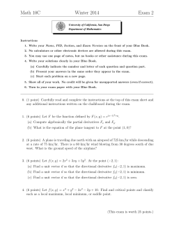
Following [3], consider a nonholonomic car-like robot with rear-wheel driving as depicted in Figure 1. The
dynamics of the system is
x˙ = v1 cos θ
y˙ = v1 sin θ
θ˙ = v1 (tan φ)/ℓ
φ˙ = v2
6
MAE281b – Nonlinear Control
c 2008-2015 by Jorge Cort´
Copyright es. Permission is granted to copy, distribute and modify this file, provided that the
original source is acknowledged.
3.1
An illustrative example: a car-like robot
3
WHAT IF NO RELATIVE DEGREE EXISTS?
Here (x, y) are the coordinates of the center of mass of the rear wheel axis, v1 is the driving velocity input
and v2 is the steering velocity input. Note that, with x
˜ = (x, y, θ, φ), g1 = (cos θ, sin θ, tan φ/ℓ, 0) and
g2 = (0, 0, 0, 1), the system can be written as
x
˜˙ = v1 g1 (˜
x) + v2 g2 (˜
x).
Figure 1: Nonholonomic car-like robot
For trajectory tracking problems, the natural outputs to consider are the position coordinates
h1 (x, y, θ, φ) = x,
h2 (x, y, θ, φ) = y.
Let us compute the relative degree of the system. Note that f = 0. Therefore, we have
Lg1 h1 = cos θ,
Lg2 h1 = 0,
Lg1 h2 = sin θ,
Lg2 h2 = 0.
Since the matrix
A(x) =
cos θ
sin θ
0
0
is singular, we conclude that the system does not have a vector relative degree. Looking at the example a
bit closer, one can realize that the reason for this is that the input v1 appears in both output derivatives,
while the input v2 appears in none. So, an idea to fix this problem is to somehow make the input v1 appear
“later” (i.e., in higher-order derivatives of the outputs) and hope that the other input will catch up. How
can we do this? Let us try using
v1 = ζ
ζ˙ = u1
7
MAE281b – Nonlinear Control
c 2008-2015 by Jorge Cort´
Copyright es. Permission is granted to copy, distribute and modify this file, provided that the
original source is acknowledged.
3.1
An illustrative example: a car-like robot
3
WHAT IF NO RELATIVE DEGREE EXISTS?
This equation extends the state of the system to (x, y, θ, φ, ζ). The control vector fields are therefore
g1 = (0, 0, 0, 0, 1) and g2 = (0, 0, 0, 1, 0). Note now that we have introduced a drift vector field f =
(ζ cos θ, ζ sin θ, ζ tan φ/ℓ, 0, 0). Now, the inputs do not appear in the first-order derivatives of the outputs,
Lg2 h1 = 0,
Lg2 h2 = 0.
Lg1 h1 = 0,
Lg1 h2 = 0,
Let us see about the second-order derivatives. We compute
Lf h1 = ζ cos θ
Lf h2 = ζ sin θ
and then we have
Lg 2 Lf h 1 = 0
Lg 2 Lf h 2 = 0
Lg1 Lf h1 = cos θ,
Lg1 Lf h2 = sin θ,
and we again have the same problem, as before, i.e., the input u1 appears earlier than the input v2 . Let us
try with one more integrator
u1 = ν
ν˙ = r1
Therefore, the extended state is now (x, y, θ, φ, ζ, ν), the inputs are r1 and v2 , and the vector fields are
f = (ζ cos θ, ζ sin θ, ζ tan φ/ℓ, 0, ν, 0), g1 = (0, 0, 0, 0, 0, 1), and g2 = (0, 0, 0, 1, 0, 0). Let us see if we finally got
what we were looking for. The inputs do not appear in the first-order derivatives of the outputs
Lg2 h1 = 0,
Lg2 h2 = 0.
Lg1 h1 = 0,
Lg1 h2 = 0,
Additionally,
Lf h1 = ζ cos θ
Lf h2 = ζ sin θ
The inputs do not appear either in the second-order derivatives of the outputs
Lg1 Lf h1 = 0,
Lg 2 Lf h 1 = 0
Lg1 Lf h2 = 0,
Lg 2 Lf h 2 = 0
Additionally,
L2f h1 = ν cos θ − ζ 2 sin θ tan φ/ℓ
L2f h2 = ν sin θ + ζ 2 cos θ tan φ/ℓ
The third-order derivatives of the outputs now look like
Lg1 L2f h1 = cos θ,
Lg1 L2f h2 = sin θ,
sin θ
ℓ cos2 φ
cos θ
Lg2 L2f h2 = ζ 2
ℓ cos2 φ
Lg2 L2f h1 = −ζ 2
8
MAE281b – Nonlinear Control
c 2008-2015 by Jorge Cort´
Copyright es. Permission is granted to copy, distribute and modify this file, provided that the
original source is acknowledged.
3.2
Achieving relative degree via dynamic extension
3
WHAT IF NO RELATIVE DEGREE EXISTS?
The determinant of the matrix
A=
Lg1 L2f h1
Lg1 L2f h2
Lg2 L2f h1
Lg2 L2f h2
is
det(A) = ζ 2
1
ℓ cos2 φ
Therefore, so long as ζ 6= 0 and φ 6= ±π/2, 3π/2, the matrix A is invertible, and the system has vector relative
degree (3, 3). Note that ρ = 3 + 3 = 6, which is the dimension of the extended state (x, y, θ, φ, ζ, ν). So, by
extending the state of the system and introducing carefully-chosen integrators, we are able to fully linearize
the system. Doing control design, e.g., trajectory tracking, is now reasonably straightforward (although care
must be taken to ensure the system stays within the domain identified above). Note that we have fully
linearized the system not through a static state feedback controller, but through a dynamic state feedback
controller. The question is, can this be done in general? Can we write our procedure in general terms? This
is what we address next.
3.2
Achieving relative degree via dynamic extension
The purpose of this section is to show that, under certain assumptions, it is possible to modify a system
which does not have a vector relative degree into a new system which does. This cannot be achieved by static
state feedback. Instead, we use a dynamic state feedback,
u = α(x, ζ) + β(x, ζ)v
ζ˙ = γ(x, ζ) + δ(x, ζ)v
This dynamic feedback is said to be a regularizing dynamic extension for (1) if the composite system has a
vector relative degree.
The basic idea of the dynamic extension algorithm is to add integrators at the appropriate places to delay
the appearances of inputs and make the system have a vector relative degree, in essentially the same way we
have done in the car-like robot example. The following formulation of the dynamic extension algorithm is
iterative. It tries to take care of problems one step at a time.
Dynamic extension algorithm: Suppose that the matrix A(x) in (2) has constant rank p < m (because
the inequality is strict, the system does not have a vector relative degree). Let ai , i ∈ {1, . . . , m} denote the
ith row of A(x). Without loss of generality (rearranging the order of the output channels if necessary), it is
possible to find smooth functions c1 , . . . , cp such that
ap+1 (x) =
p
X
ci (x)ai (x).
i=1
% This fact is not good for achieving a relative degree. Somehow, some input has appeared a bit
too soon when deriving one of the first p outputs
It must be the case that there exists i0 ∈ {1, . . . , p} and j0 ∈ {1, . . . , m} such that
ρ
ai0 j0 = Lgj0 Lfi0
−1
hi0 6= 0.
% The input j0 is the culprit (or at least, it is one of them). Let us make it show up later in the
derivatives of the output i0 using an integrator.
9
MAE281b – Nonlinear Control
c 2008-2015 by Jorge Cort´
Copyright es. Permission is granted to copy, distribute and modify this file, provided that the
original source is acknowledged.
3.2
Achieving relative degree via dynamic extension
3
WHAT IF NO RELATIVE DEGREE EXISTS?
Let us then define
uj = v j ,
u j0 =
1
ai0 j0
j 6= j0
(5a)
ρ
− Lfi0 hi0 + ζ −
m
X
ai0 j vj
j=1
j6=j0
(5b)
ζ˙ = vj0
(5c)
% What do we achieve with this? Basically, we delay the appearance of the input j0 when making
derivatives of the output hi0 .
With this choice, we now have
(ρ
)
m
X
ρ
−1
= Lfi0 hi0 + ai0 j0 uj0 +
m
X
ρ
yi0 i0 = Lfi0 hi0 +
L g j L f i0
hi0 uj
j=1
ρ
ai0 j uj = ζ
j=1
j6=j0
Therefore, in the system with state (x, ζ), the first time an input appears in the derivatives of the output hj0
is when we do the ρi0 + 1 derivative,
(ρ
yi0 i0
+1)
= ζ˙ = vj0
% So this is what we have accomplished: now the input j0 appears “one derivative later.” The
hope is that this will make the resulting matrix A invertible. Otherwise, we repeat the process.
As a result of the addition of the integrator, the system we are dealing with now has state (x, ζ) of dimension
n + 1,
x˙ = f (x) +
X
j=1
j6=j0
vj gj (x) + gj0 (x)
1
ai0 j0
ρ
− Lfi0 hi0 + ζ −
m
X
j=1
j6=j0
ai0 j vj
ζ˙ = vj0
(6a)
(6b)
y1 = h1 (x)
..
.
ym = hm (x)
(6c)
(6d)
If this system has a relative degree, then the algorithm terminates. Otherwise, we repeat the procedure
starting with (6).
In general, we have no guarantee that the dynamic extension algorithm will succeed. However, if it does,
then the regularizing dynamic feedback it generates has necessarily the least possible dimension. This fact is
a consequence of the following result.
Proposition 3.1 Suppose the dynamic extension algorithm has been iterated k times. Let
u = H(x, ζ) + K(x, ζ)˜
v
ζ˙ = F (x, ζ) + G(x, ζ)˜
v
(7a)
(7b)
10
MAE281b – Nonlinear Control
c 2008-2015 by Jorge Cort´
Copyright es. Permission is granted to copy, distribute and modify this file, provided that the
original source is acknowledged.
REFERENCES
REFERENCES
with ζ ∈ Rk denote the composition of the k feedback laws of the form (5) constructed at each stage of the
algorithm. On the other hand, assume there exists a regularizing dynamic extension
u = H(x, ν) + K(x, ν)v
(8a)
ν˙ = F (x, ν) + G(x, ν)v
(8b)
with ν ∈ Rℓ . Then k ≤ ℓ, and the feedback (8) is the result of the composition of the feedback (7) with an
additional regularizing dynamic extension of the form
˜ ζ, z)v
v˜ = α
˜ (x, ζ, z) + β(x,
˜ ζ, z)v
z˙ = γ˜ (x, ζ, z) + δ(x,
with z ∈ Rℓ−k .
Interestingly enough, it is currently an open problem to come up with sufficient and necessary conditions that
guarantee that a system can be linearized by means of dynamic state feedback. In other words, an equivalent
of Theorem 2.9 is not known for the dynamic feedback case, although partial results are available.
References
[1] A. Isidori, Nonlinear Control Systems, 3rd ed., ser. Communications and Control Engineering Series.
1995.
Springer,
[2] W. Respondek, “Geometry of static and dynamic feedback,” lectures given at the Summer Schools on Mathematical
Control Theory, Trieste, Italy, September 2001, and Bedlewo, Poland, September 2002.
[3] A. D. Luca, G. Oriolo, and C. Samson, “Feedback control of a nonholonomic car-like robot,” in Robot Motion
Planning and Control, J.-P. Laumond, Ed. New York: Springer, 1998, pp. 171–253.
11
MAE281b – Nonlinear Control
c 2008-2015 by Jorge Cort´
Copyright es. Permission is granted to copy, distribute and modify this file, provided that the
original source is acknowledged.