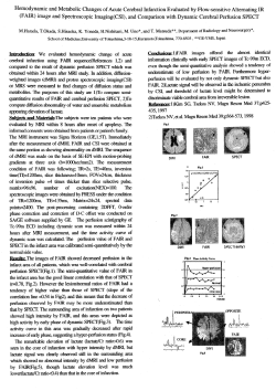
Computers & Graphics 35 (2011) 160–174
Contents lists available at ScienceDirect
Computers & Graphics
journal homepage: www.elsevier.com/locate/cag
Technical Section
Scale-dependent and example-based grayscale stippling
Domingo Martı́n a,, Germán Arroyo a, M. Victoria Luzón a, Tobias Isenberg b,c
a
b
c
University of Granada, Spain
University of Groningen, The Netherlands
DIGITEO & CNRS/INRIA, France
a r t i c l e i n f o
a b s t r a c t
Available online 15 November 2010
We present an example-based approach to synthesizing stipple illustrations for static 2D images that
produces scale-dependent results appropriate for an intended spatial output size and resolution. We
show how treating stippling as a grayscale process allows us to both produce on-screen output and to
achieve stipple merging at medium tonal ranges. At the same time we can also produce images with high
spatial and low color resolution for print reproduction. In addition, we discuss how to incorporate highlevel illustration considerations into the stippling process based on discussions with and observations of a
stipple artist. Also, certain features such as edges can be extracted and used to control the placement of
dots to improve the result. The implementation of the technique is based on a fast method for distributing
dots using halftoning and can be used to create stipple images interactively. We describe both a GPU
implementation of the basic algorithm that creates stipple images in real-time for large images and an
extended CPU method that allows a ﬁner control of the output at interactive rates.
& 2010 Elsevier Ltd. All rights reserved.
Keywords:
Stippling
High-quality rendering
Scale-dependent NPR
Example-based techniques
Illustrative visualization
1. Introduction
Stippling is a traditional pen-and-ink technique that is popular
for creating illustrations in many domains. It relies on placing
stipples (small dots that are created with a pen) on a medium such
as paper such that the dots represent shading, material, and
structure of the depicted objects. Stippling is frequently used by
professional illustrators for creating illustrations, for example, in
archeology (e.g., see Fig. 2), entomology, ornithology, and botany.
One of the essential advantages of stippling that it shares with
other pen-and-ink techniques is that it can be used in the common
bilevel printing process. By treating the stipple dots as completely
black marks on a white background they can easily be reproduced
without losing spatial precision due to halftoning artifacts. This
property and the simplicity of the dot as the main rendering element
has lead to numerous approaches to synthesize stippling within NonPhotorealistic Rendering (NPR), describing techniques for distributing
stipple dots such that they represent a given tone. Unfortunately,
computer-generated stippling sometimes creates distributions with
artifacts such as unwanted lines, needs a lot of computation power
due to the involved computational complexity of the approaches,
cannot re-create the merging of stipple dots in middle tonal ranges
that characterizes many hand-drawn examples, or produces output
with dense stipple points unlike those of hand-drawn illustrations.
To address these issues, our goal is to realize a stippling process for
2D images (see example result in Fig. 1) that is easy to implement, that
Corresponding author. Tel.: +34 958240578; fax: + 34 958243179.
E-mail address: [email protected] (D.R. Martı́n).
0097-8493/$ - see front matter & 2010 Elsevier Ltd. All rights reserved.
doi:10.1016/j.cag.2010.11.006
considers the whole process of hand-made stippling, and that takes
scale and output devices into account. For this purpose we do not
consider stippling to always be a black-and-white technique, in
contrast to previous NPR approaches (e.g., [1]). In fact, we use the
grayscale properties of hand-made stipple illustrations to inform the
design of a grayscale stipple process. This different approach lets us
solve not only the stipple merging problem but also lets us create
output adapted to the intended output device. To summarize, our
paper makes the following contributions:
an analysis of high-level processes involved in stippling and a
discussion on how to support these using image-processing,
a method for example-based stippling in which the stipple dot
placement is based on halftoning,
the scale-dependent treatment of scanned stipple dot examples,
desired output, and stipple placement,
a grayscale stippling process that can faithfully reproduce the
merging of stipples at middle tonal ranges,
the enabling of both print output in black-and-white and on
screen display in gray or tonal scales at the appropriate spatial
and color resolutions,
an optional special treatment of image edges that improves the
control of the placement of stipples,
a technique that is easy to implement and permits the interactive creation of stipple images,
a description of a GPU implementation of the basic technique, and
a comparative analysis of the stipple dot placement statistics for
both the hand-drawn example and generated synthetic stipple
images.
D. Martı́n et al. / Computers & Graphics 35 (2011) 160–174
Fig. 1. An example stipple image created with our technique.
This article is an extended version of a paper [2] published at
NPAR 2010. The remainder is structured as follows. First we review
related work in the context of computer-generated stippling in
Section 2. Next, we analyze hand-made stippling in Section 3, both
with respect to high-level processes performed by the illustrator
and low-level properties of the stipple dots. Based on this analysis
we describe our scale-dependent grayscale stippling process in
Section 4. We analyze the performance and describe a GPU
implementation in Section 5, before discussing the results in
Section 6. We conclude the paper and suggest some ideas for
future work in Section 7.
2. Related work
Pen-and-ink rendering and, speciﬁcally, computer-generated
stippling are well-examined areas within NPR. Many approaches
exist to both replicating the appearance of hand-drawn stipple
illustrations and using stippling within new contexts such as
animation. In the following discussion we distinguish between
stipple rendering based on 3D models such as boundary representations or volumetric data on the one side and stippling that
uses 2D pixel images as input on the other.
The variety of types of 3D models used in computer graphics is also
reﬂected in the diversity of stipple rendering approaches designed for
them. There exist techniques for stippling of volume data [3,4]
typically aimed at visualization applications, stipple methods for
implicit surfaces [5,6], point-sampled surfaces [7,8], and stippling of
polygonal surfaces [9,10]. The placement of stipple dots in 3D space
creates a unique challenge for these techniques because the viewer
ultimately perceives the point distribution on the 2D plane. Related to
this issue, animation of stippled surfaces [11,12] presents an additional challenge as the stipples have to properly move with the
changing object surface to avoid the shower-door effect. A special case
of stippling of 3D models is the computation in a geometry-image
domain [13] where the stippling is computed on a 2D geometry image
onto which the 3D surface is mapped.
While Yuan et al. [13] map the computed stipples back onto the
3D surface, many approaches compute stippling only on 2D pixel
images. The challenge here is to achieve an evenly spaced
distribution that also reﬂects the gray value of the image to be
represented, an optimization problem within stroke-based rendering [14]. One way to achieve a desired distribution is Lloyd’s
method [15,16] that is based on iteratively computing the centroidal Voronoi diagram (CVD) of a point distribution. Deussen et al.
[17] apply this technique to locally adjust the point spacing
through interactive brushes, starting from initial point distribution
—generated, e.g., by random sampling or halftoning—in which the
point density reﬂects the intended gray values. The interactive but
161
local application addresses a number of problems: the computational complexity of the technique as well as the issue that
automatically processing the entire image would simply lead to
a completely evenly distributed set of points. Thus, to allow
automatic processing while maintaining the desired density,
Secord [18] uses weighted Voronoi diagrams to reﬂect the intended
local point density. A related way of achieving stipple placement
was explored by Schlechtweg et al. [19] using a multi-agent system
whose RenderBots evaluate their local neighborhood and try to
move such that they optimize spacing to nearby agents with
respect to the desired point density.
Besides evenly spaced distributions it is sometimes desirable to
achieve different dot patterns. For instance, Mould [20] employs a
distance-based path search in a weighted regular graph that
ensures that stipple chains are placed along meaningful edges in
the image. In another example, Kim et al. [21] use a constrained
version of Lloyd’s method to the arrange stipples along offset lines
to illustrate images of faces. However, in most cases the distribution should not contain patterns such as chains of stipple
points—professional illustrators speciﬁcally aim to avoid these
artifacts. Thus, Kopf et al. [22] use Wang-tiling to arrange stipple
tiles in large, non-repetitive ways and show how to provide a
continuous level of detail while maintaining blue noise properties.
This means that one can zoom into a stipple image with new points
continuously being added to maintain the desired point density.
In addition to stipple placement, another issue that has previously been addressed is the shape of stipple points. While most
early methods use circles or rounded shapes to represent stipples
[17,18], several techniques have since been developed for other
shapes, adapting Lloyd’s method accordingly [23], using a probability density function [24], or employing spectral packing [25].
It is also interesting to examine the differences between computer-generated stipple images and hand-drawn examples. For example, Isenberg et al. [26] used an ethnographic pile-sorting approach to
learn what people thought about both and what differences they
perceive. They found that both the perfectly round shapes of stipple
dots and the artifacts in placing them can give computer-generated
images away as such, but also that people still valued them due to
their precision and detail. Looking speciﬁcally at the statistics of
stipple distributions, Maciejewski et al. [27] quantiﬁed these differences with statistical texture measures and found that, for example,
computer-generated stippling exhibits an undesired spatial correlation away from the stipple points and a lack of correlation close to
them. This lead to the exploration of example-based stippling, for
instance, by Kim et al. [1]. They employ the same statistical evaluation
as Maciejewski et al. [27] and use it to generate new stipple
distributions that have the same statistical properties as hand-drawn
examples. By then placing scanned stipple dots onto the synthesized
positions Kim et al. [1] are able to generate convincing stipple
illustrations. However, because the technique relies on being able
to identify the centers of stipple points in the hand-drawn examples it
has problems with middle tonal ranges because there stipple dots
merge into larger conglomerates.
This issue of stipple merging in the middle tonal ranges is one
problem that remains to be solved. In addition, while computergenerated stippling thus far has addressed stipple dot placement,
stipple dot shapes, and animation, other aspects such as how to
change an input image to create more powerful results (i.e., how to
interpret the input image) have not yet been addressed.
3. Analysis of hand-drawn stippling
To inform our technical approach for generating high-quality
computer-generated stipple illustrations, we start by analyzing the
process professional stipple illustrators perform when creating a
162
D. Martı́n et al. / Computers & Graphics 35 (2011) 160–174
drawing. For this purpose we involved a professional stipple artist
and asked her to explain her approach/process using the example
illustration shown in Fig. 2. From this analysis we extract a number
of speciﬁc high-level processes that are often employed by
professional stipple artists that go beyond simple dot placement
and use of speciﬁc dot shapes. We discuss these in Section 3.1
before analyzing the low-level properties of stipple dots in Section
3.2 that guide our synthesis process.
3.1. High-level processes
The manual stipple process has previously been analyzed to
inform computer-generated stippling. As part of this analysis and
guided by literature on scientiﬁc illustration (e.g., [28]), researchers
identiﬁed an even distribution of stipple points as one of the major
goals (e.g., [17,18]) as well as the removal of artifacts (e.g., [22,27]).
Also, Kim et al. [1] noted the use of tone maps by illustrators to
Fig. 2. Hand-drawn stipple image by illustrator Elena Piñar of the Roman theater of Acinipo in Ronda, Málaga (originally on A4 paper). This image is s 2009 Elena Piñar, used
with permission.
Fig. 3. Original photograph and interpreted regions for Fig. 2. (a) Original photograph, Roman theater of Acinipo in Ronda, Málaga. (b) Interpreted regions.
D. Martı́n et al. / Computers & Graphics 35 (2011) 160–174
guide the correct reproduction of tone. While these aspects of
stippling concentrate on rather low-level properties, there are also
higher-level processes that stipple artists often employ in their
work. Artists apply prior knowledge about good practices, knowledge about shapes and properties of the depicted objects, knowledge about the interaction of light with surfaces, and knowledge
about the goal of the illustration. This leads to an interpretation of
the original image or scene, meaning that stippling goes beyond an
automatic and algorithmic tonal reproduction.
To explore these processes further we asked Elena Piñar, a
professional illustrator, to create a stipple illustration (Fig. 2) from a
digital photo (Fig. 3(a)). We observed and video-recorded her work
on this illustration and also met with her afterwards to discuss her
work and process. In this interview we asked her to explain the
approach she took and the techniques she employed. From this
conversation with her we could identify the following higher-level
processes (see Fig. 3 for a visual explanation with respect to the
hand-made illustration in Fig. 2 and photograph in Fig. 3(a)). While
this list is not comprehensive, according to Elena Piñar it comprises
the most commonly used and most important techniques (some of
these are mentioned, e.g., by Guptill [29]). Also, each artist has his
or her own set of techniques as part of their own personal style.
Abstraction: One of the most commonly used techniques is
removing certain parts or details in the image to focus the
observer’s attention on more important areas. In our example,
the sky and some parts of the landscape have been fully removed
(shown in violet in Fig. 3(b)). In addition, removing areas contributes to a better image contrast.
Increase in contrast: Some parts of the original color image
exhibit a low level of contrast, reducing their readability when
stippled. To avoid this problem illustrators increase the contrast in
such regions (green area) through global and local evaluation of
lightness, enhancing the detail where necessary.
Irregular but smoothly shaped outlines: If objects in an image are
depicted with a regular or rectilinear shape they are often
perceived as being man-made. To avoid this impression for natural
shapes, stipple artists eliminate parts of these objects to produce an
irregular form and add a tonal gradient (yellow).
Reduction of complexity: It is not always possible to remove all
unimportant areas. In these cases the complexity or amount of
detail is reduced. This effect is shown in orange in Fig. 3(b): the
artist has removed some small parts that do not contribute to the
illustration’s intended message.
Additional detail: As visible in the red areas in Fig. 3(b), some
parts that are not (or not clearly) visible in the original are still
shown in the illustration. Here, the illustrator has enhanced details
of the rocks based on her prior knowledge.
Inversion: Sometimes artists convert very dark zones or edges
into very clear ones to improve the contrast. This technique is
applied subjectively to speciﬁc parts of the drawing rather than to
the image as a whole. In the hand-made stippled drawing the
cracks between rocks are shown in white while they are black in the
original photograph (blue in Fig. 3(b)).
Despite the fact that these high-level processes are an integral part
of hand-drawn stipple illustration, computer-generated stippling
techniques have largely concentrated on dot placement and dot
shapes. This is understandable as these low-level processes can be
automated while the higher-level processes to a large degree rely on
human intelligence and sense of aesthetics. To be able to incorporate
higher-level interpretations of images, therefore, we manually apply
global and local image processing operations to the input image
(Fig. 4). Instead of directly using a gray-level input image (Fig. 4(a)) we
ﬁrst apply pre-processing to accommodate the identiﬁed high-level
processes. Following the list of processes given above (see Fig. 4(b)),
we remove non-relevant parts from the image such as the sky and
parts of the background. Also, we increase the contrast globally but
163
Fig. 4. Deriving the helper image to capture the high-level stippling processes.
(a) Grayscale version of Fig. 3(a). (b) Adjusting global contrast and local detail of (a).
(c) Manually added edges, inversion, local contrast.
also increase the brightness of some regions locally. Next, we locally
delete parts of natural objects and smooth the border of these regions.
To reduce the complexity of certain parts such as the metal grid we
select these regions and apply a large degree of blur. Adding elements
based on previous knowledge typically requires the artist painting
into the image. Some additional information, however, can be added
with algorithmic support, in particular edges that border regions that
are similar in brightness such as the top borders of the ruin. We
164
D. Martı́n et al. / Computers & Graphics 35 (2011) 160–174
Fig. 5. Enlarged hand-drawn stipple dots (scanned at 1200 ppi).
support this by either extracting an edge image from the original color
image, taking only regions into account that have not been deleted in
Fig. 4(b) and adding them to the helper image. Alternatively, artists
can manually draw the necessary edges as shown in Fig. 4(c). Finally,
inversion can be achieved by also manually drawing the intended
inverted edges as white lines into the touched-up grayscale image
(see Fig. 4(c)).
While this interactive pre-processing could be included into a
comprehensive stipple illustration tool, we apply the manipulations using a regular image processing suite (e.g., Adobe Photoshop
or GIMP). This allows us to make use of a great variety of image
manipulation tools and effects to give us freedom to achieve the
desired effects. The remainder of the process, on the other hand, is
implemented in a dedicated tool. Before discussing our algorithm
in detail, however, we ﬁrst discuss some low-level aspects of handdrawn stipple dots that are relevant for the approach.
Fig. 6. Basic process: one black pixel in the halftoning image is converted to one dot
in the ﬁnal image.
4. A grayscale stippling process
Based on the previous analysis we now present our process for
high-quality example-based stippling. In contrast to previous
approaches, our process captures and maintains the stipple image
throughout the entire process as high-resolution grayscale image,
which allows us to achieve both stipple merging for the middle
tonal ranges and high-quality print output. Also, to allow for
interactive control of the technique, we use Ostromoukhov’s [30]
fast error-diffusion halftoning technique to place the stipples.
Below we step through the whole process by explaining the stipple
placement (Section 4.1), the stipple dot selection and accumulation
(Section 4.2), and the generation of both print and on-screen output
(Section 4.3). In addition, we discuss adaptations for interactive
processing (Section 4.4).
3.2. Low-level properties of stipple dots
4.1. Stipple dot placement using halftoning
Stipple dots and their shapes have been analyzed and used in
many previous computer stippling techniques, inspired by the
traditional hand-drawn stippling. Hodges [28] notes that each dot
should have a purpose and that dots should not become dashes. In
computer-generated stippling, therefore, dots have typically been
represented as circular or rounded shapes1 or pixels that are placed
as black elements on a white ground. However, each use of a pen to
place a dot creates a unique shape (e.g., Fig. 5) which is partially
responsible for the individual characteristics of a hand-made
stipple illustration. Thus, recent computer-generated stippling
employed scans of dots from hand-made illustrations to better
capture the characteristics of hand-drawn stippling [1].
We follow a similar approach and collected a database of stipple
points from a high-resolution scan of a hand-drawn original
illustration, a sample of which is shown in Fig. 5. These stipple
dots are not all equal but have varying shapes and sizes. One can
also notice that the stipples are not completely black but do exhibit
a grayscale texture. This texture is likely due to the speciﬁc
interaction of the pen’s ink with the paper and typically disappears
when the stipple illustration is reproduced in a printing process.
This lead to the assumption that stipple dots are always completely
black marks on a white background as used in much of the previous
literature. However, the grayscale properties of real stipple dots are
a characteristic of the real stippling process which one may want to
reproduce provided that one employs an appropriate reproduction
technology. In addition, we also make use of these grayscale
properties for realizing a technique that can address one of the
remaining challenges in stippling: the merging of dots in the
middle tonal ranges.
Our stippling process starts by obtaining a grayscale version of
the target image using the techniques described in Section 3.1. In
principle, we use this image to run Ostromoukhov’s [30] errordiffusion technique to derive locations for placing stipple dots,
similar to the use of halftoning to determine the starting distribution in the work by Deussen et al. [17]. However, in contrast to their
approach that adds point relaxation based on Lloyd’s method, we
use the locations derived from the halftoning directly which allows
us to let stipple dots merge, unlike the results from relaxation (see
Fig. 6). The reason for choosing a halftoning technique over, for
example, distributions based on hand-drawn stipple statistics [1] is
twofold. The main reason is that halftoning has the evaluation of
tone built-in so that it does not require a tone map being extracted
from the hand-drawn example. The second reason lies in that
halftoning provides a continuum of pixel density representing
tonal changes as opposed to the approach of using both black pixels
on a white background for brighter regions and white pixels on a
black background for darker areas as used by Kim et al. [1].
Speciﬁcally, we are employing Ostromoukhov’s [30] errordiffusion, partially because it is easy to implement and produces
results at interactive frame-rates. More importantly, however, the
resulting point distributions have blue noise properties, a quality
also desired by related approaches [22]. This means that the result
is nearly free of dot pattern artifacts that are present in results
produced by many other error-diffusion techniques, a quality that
is important for stippling [28].
Using a halftoning approach, however, means that we produce a
point distribution based on pixels that are arranged on a regular grid, in
contrast to stipples that can be placed at arbitrary positions. In addition,
we cannot use the grayscale input image in the same resolution as the
intended output resolution for the stipple image. Let us use an example
to better explain this problem and describe its solution. Suppose we
1
Aside from more complex artiﬁcial shapes that have also been used but that
are not necessarily inspired by hand-drawn stippling, see Section 2.
D. Martı́n et al. / Computers & Graphics 35 (2011) 160–174
165
Fig. 8. Magniﬁed comparison of stipple placement before and after random
perturbation of the stipple locations. (a) Grid placement of stipples. (b) After
random perturbation.
Fig. 7. Effect of the packing factor.
have a hand-stippled A4 image (in landscape) that we scan for analysis
and extraction of stipple dot examples at 1200 ppi.2 This means that
the resulting image has roughly 14,000 10,000 pixels, with stipple
dot sizes ranging from approximately 10 10 to 20 20 pixels.3 If we
now were to produce an equivalent A4 output image at 1200 ppi,
would hence use an 14,000 10,000 pixel grayscale image, and
compute its halftoned version at this size, each pixel in this image
would represent one dot. This means we would need to place scanned
stipple dots (whose average size is 16 16 pixels, this is equivalent to a
spatial size of 0.338 mm, slightly larger than the nominal size of
0.2 mm of the tip of the used pen) at the pixel locations of the halftoned
image. Consequently, this would produce a result that is 16 larger
than the intended output image and reproducing it at A4 size would
result in the characteristics of the stipple dot shapes being lost because
each stipple would again be shrunken down to the size of approximately one pixel.
Therefore, for a given output resolution reso we compute the dot
distribution using error-diffusion halftoning at a smaller halftoning
resolution resht, which implies that the halftoning image must be
obtained by scaling the input image. The value of the scaling is the
halftoning factor fht. Intuitively for our 1200 ppi example, one could
suggest a halftoning factor fht whose value is 1/16 of reso to compute
resht, using the average stipple’s diameter of 16 pixels:
resht ¼ fht reso ;
fht ¼ 1=16;
reso ¼ 1200 ppi:
ð1Þ
In a completely black region and for ideally circular stipples,
however, this would result in a pattern of white spots because
the black dots on the
pﬃﬃﬃgrid only touch. To avoid this issue one has to
use a factor fht of 2=16 to allow for a denser packing of stipple
points such that they overlap (see Fig. 7). For realistic stipple points
with non-circular shapes one may even have to use a fht of 2/16 or
more. On the other hand, even in the darkest regions in our example
the stipple density is not such that they completely cover the
canvas. Thus, we leave this choice up to the user to decide how
dense to pack the stipples, and introduce a packing factor fp to be
multiplied with fht to control the density of the stipples:
fht ¼ fp =16:
ð2Þ
For fp ¼1 and, thus, fht ¼1/16 we would perform the halftoning in
our example on an image with size 875 625 pixels to eventually
yield a 1200 ppi landscape A4 output. For other output resolutions,
however, the situation is different. Because the stipples have to use
2
Please notice that ppi stands for pixels per inch and is used intentionally while
dots per inch (dpi) is used when we discuss printing.
3
These values are derived from the example in Fig. 2 (done with a pen with a
0.2 mm tip) and can be assumed to be valid for many stipple images as similar pen
sizes are used by professional illustrators [28].
proportionally smaller pixel sizes for smaller resolutions to be
reproduced at the same spatial sizes, the factor between output
image and halftoning image has to change proportionally as well.
For example, for a 600 ppi output resolution the average stipple’s
diameter would only be 8 pixels, and consequently fht would only
be 1/8. Thus, we can derive the halftoning resolution resht for a
given output resolution reso in ppi based on the observations we
made from scanning a sample at 1200 ppi as follows:
resht ¼ fht reso ;
fht ¼
fp 1200 ppi
16 reso
resht ¼ 75 ppi fp :
ð3Þ
This means that the halftoning resolution is, in fact, independent of
the output resolution. Consequently, the pixel size of the halftoning
image only depends on the spatial size of the intended output and
the chosen packing factor (and ultimately the chosen scanned
example stippling whose stipple dot size depends on the used pen).
This leaves the other mentioned problem that arises from
computing the stipple distribution through halftoning: the stipple
dots would be arranged on a regular grid, their centers always being
at the centers of the pixels from the halftoning image. To avoid this
issue, we perturb the locations of the stipple dots by a random
proportion of between 0 and 7100% of their average diameter, in
both x- and y-direction. Together with the random selection of
stipple sizes from the database of scanned stipples and the blue
noise quality of the dot distribution due to the chosen halftoning
technique this successfully eliminates most observable patterns in
dot placement (see Fig. 8).
4.2. Stipple dot selection and accumulation
We begin the collection of computed stipple points by creating a
grayscale output buffer of the desired resolution, with all pixels
having been assigned the full intensity (i.e., white). Then we derive the
stipple placement by re-scaling the modiﬁed grayscale image to the
halftoning resolution and running the error-diffusion as described in
the previous section. Based on the resulting halftoned image and the
mentioned random perturbations we can now derive stipple location
with respect to the full resolution of the output buffer.
For each computed location we randomly select a dot from the
previously collected database of stipple dot scans. This database is
organized by approximate stipple dot sizes, so that for each
location we ﬁrst determine the size class using a random function
that follows a uniform distribution (all the sizes have the same
probability) or a normal distribution centered on the average size,
and then randomly select a speciﬁc dot from this class. The
selection of which random function to use is of aesthetic nature
and left up to the user. The default random function uses the
uniform distribution, producing a less regular result. The selected
dot is then added to the output buffer, combining intensities of the
new stipple dot is and the pixels previously placed into the buffer ibg
166
D. Martı́n et al. / Computers & Graphics 35 (2011) 160–174
using ðis ibg Þ=255 (for 8 bits). This not only ensures that stipples
placed on a white background are represented faithfully but also
that the result gets darker if two dark pixels are combined
(accumulation of ink; for example, given is ¼45 and ibg ¼64, the
result is 11 which is darker than the original values).
Both the range of stipple sizes and the partially random stipple
placement ensure that stipples can overlap. This overlapping is
essential for our approach, it ensures the gradual merging of
stipples into larger conglomerates as darker tones are reproduced
(see example in Fig. 9). Therefore, we can for the ﬁrst time simulate
this aspect of the aesthetics of hand-drawn stippling.
halftoning [31]. In contrast, for on-screen display it does not make
sense to generate a very high-resolution image because this cannot
be seen on the screen.
Fig. 12. High-resolution dots (left) and their ‘posterized’ versions (right) for
determining the dots’ visual centers.
4.3. Generation of print and screen output
One challenge that remains is to generate the appropriate
output for the intended device. Here we typically have two options:
on-screen display and traditional print reproduction. These two
options for output differ primarily in their spatial resolution and
their color resolution. While normal bilevel printing offers a high
spatial resolution (e.g., 1200 dpi), it has an extremely low color
resolution (1 bit or 2 bit) while typical displays have a lower spatial
resolution (approximately 100 ppi) but a higher color resolution
(e.g., 8 bit or 256 bit per primary). These differences also affect the
goals for generating stipple illustrations. For example, it does not
make much sense to print a grayscale stipple image because the
properties of the individual stipple points (shape, grayscale texture) cannot be reproduced by most printing technology, they
would disappear behind the pattern generated by the printer’s
Fig. 13. Scaling problem with nonhorizontal straight lines.
Random
numbers
Halftoning
image
Stippling
points
library
Fig. 9. Merging of synthesized stipples at two tonal ranges. (a) Lighter region.
(b) Darker region.
(a)
(b)
Blending
(c)
FBO 1
FBO 2
Blending
Fig. 10. Details of the 1200 ppi outputs with the grayscale, black and white, and
halftoning process. (a) Grayscale. (b) Black and white. (c) Dithered.
Fig. 14. Three textures are passed to a fragment shader program: the halftoning, the
stippling points, and a texture containing random values. The image is rendered into
a frame buffer object (FBO). The partial result is blended with the previous one. Two
FBOs are needed for this process because a FBO cannot feed itself.
Fig. 11. Details of the improvement in the placement of borders dots (the images of the ﬁlters are scaled). (a) Original. (b) DoG ﬁlter. (c) Improved with DoG. (d) Sobel ﬁlter.
(e) Improved with Sobel.
D. Martı́n et al. / Computers & Graphics 35 (2011) 160–174
Fig. 15. The two ﬁrst steps of the algorithm: In the 1st step (left), the algorithm
renders the dots with the necessary distance to prevent overlapping. In the 2nd step
(right), the next dots are rendered and blended to the previous step. The algorithm is
repeated until the ﬁnal illustration is complete.
167
Therefore, we adjust our stippling process according to the
desired output resolutions, both color and spatial. For output
designed for print reproduction we run the process at 1200 ppi,
using a stipple library from a 1200 ppi scan, and compute the
scaling factor for the halftoning process to place the stipples
accordingly. The resulting 1200 ppi grayscale output image is then
thresholded using a user-controlled cut-off value, and stored as a
1 bit pixel image, ready for high-quality print at up to 1200 dpi (e.g.,
Fig. 16). These images, of course, do no longer contain stipples with
a grayscale texture but instead are more closely related to printed
illustrations in books.
As a print reproduction alternative we also provide the option to
apply a dedicated halftoning step (using Ostromoukhov’s [30]
error-diffusion algorithm) to a grayscale stippling result. This
allows us to maintain the grayscale properties of the stipple dots
even in a black-and-white output medium such as print (Fig. 10).
For instance, for 1200 dpi output we can reproduce approximately
32 grayscale tones, while bypassing the problem that many
printers apply a Postscript dithering which is limited compared
to Ostromoukhov’s stochastic dithering. On sufﬁciently highresolution (1200 dpi and higher) printers, the dedicated dithering
allows us to maintain the grayscale properties of the stipple dots
while the dither pattern is close to being unnoticeable.
For on-screen display, in contrast, we run the process at a lower
resolution, e.g., 300 ppi (while 300 ppi is larger than the typical screen
Fig. 16. Example generated for A4 print reproduction at 1200 dpi resolution, using Fig. 4(c) as input.
168
D. Martı́n et al. / Computers & Graphics 35 (2011) 160–174
resolution, it also allows viewers to zoom into the stipple image to
some degree before seeing pixel artifacts). For this purpose the
stipples in the database are scaled down accordingly, and the
appropriate scaling value for the halftoning process is computed
based on average stipple size at this lower resolution. The resulting
image (e.g., Fig. 18) is smaller spatially but we preserve the texture
information of the stipples. These can then be appreciated on the
screen and potentially be colored using special palettes (e.g., sepia). In
addition, grayscale stipple images can also be used for special
continuous tone printing processes such as dye-sublimation.
4.4. User interaction
Several parameters of the process can be adjusted interactively
according to aesthetic considerations of the user, in addition to
applying the high-level processes (parallel or as pre-processing).
The most important settings are the intended (spatial) size and
output resolution because these affect the resolutions at which the
different parts of the process are performed. For example, a user
would select A5 as the output size and 300 ppi as the intended
resolution. Based on this the (pixel) resolution of both output buffer
and halftoning buffer are derived as outlined in Section 4.1. To
control the stipple density, we let the users interactively adjust the
packing factor (the default value is 2). In addition we let users
control the amount of placement randomness as a percentage of the
average size of the stipple dots (the default value is 25%). This
means that we specify the packing factor and placement randomness based on the average stipple size at the chosen resolution,
which results in visually equivalent results regardless of which
speciﬁc resolution is chosen.
4.5. Stipple dot placement improvements
Fig. 17. Comparison of stipple merging between a hand-drawn and a synthesized
sample, taken from the same region of the images. (a) Detail from Fig. 2. (b) Detail
from Fig. 16.
Of course, our general approach is not without ﬂaws. One
problem arises from the use of halftoning on a resolution lower
than the output one to derive stipple distributions because this
initially leads to the stipples being placed on a grid. While we
address this grid arrangement by introducing randomness to the
ﬁnal stipple placement, this also leads to noise being added to
otherwise clear straight lines in the input image. This effect can be
observed by comparing the upper edge of the ruin in Fig. 16 with
the same location in the hand-made example in Fig. 2 where the
line of stipple dots is nicely straight.
Fig. 18. Sepia tonal stipple example generated for A4 on-screen viewing at up to 300 ppi resolution, with slight gamma correction.
D. Martı́n et al. / Computers & Graphics 35 (2011) 160–174
Given the importance of lines and borders in the illustration
process, we address this issue by analyzing the local character of
the source image. We detect the edges in the source image using an
edge detector. These border ﬁlters produce grayscale images, with
darker values showing that borders are nearer. This value is used to
control the random displacement of the stipple dots: the degree of
the detected edge (de, value between 0 and 1) controls the
maximum random displacement, i.e., it is used as a factor for the
stipple points average diameter as used in the displacement
computation. Fig. 11 illustrates this displacement process, showing
that reducing the displacement for stipples dots on edges reduces
the noise introduced for these effects. While the improvement is
subtle in these detail images, it is more visible in complete images
(see the examples in Figs. 20 and 21). This seems to be a global
perception since the dots are better placed overall in the image,
producing a more contrasted and deﬁned result.
Speciﬁcally, we experimented with the Sobel operator [32]
because it is fast to compute and with the Difference of Gaussians
(DoG) [33] because it relates to the processing in the human
perceptual system. While there is no ideal method to compute the
borders to control the random displacement, the ones we implemented allow users to experiment with the effects by controlling
their parameters.
The control of randomness of stipple dot placement is combined
with other measures to reduce the noise on lines and borders. These
measures include more control over the sizes of the stipple dots
using a random selection that follows a normal distribution
centered around the mean dot size to ensure that most dots on a
line or border have the same mean size which maintains the
aesthetic of more regularity of stipple placement on these lines.
In addition, the dot placement needs to be controlled based on the
visual center of the scanned dot so that lined-up dots also visually
form a line. The concept of a visual center is based on the observation
that, while the scanned dots are embedded in a regular and square
grid, they do not have to have a regular shape or ink distribution and
the geometric center of the grid is not necessarily the visual center. For
example, the dot may have one main dark zone that is close to a
corner, or there may be two dark zones, etc. For computing the visual
center we use a straightforward approach—we ‘posterize’ each dot
image: First, the number of gray levels is reduced to a low number of
levels, usually between 4 and 7 (see Fig. 12). Then, the mean position
of the pixels in the darkest level is computed and recorded as the
stipple dot’s visual center.
All techniques used together allow us to improve the treatment
of borders and lines in the stipple images but still fail to solve all
issues. For example, our resolution-dependent stippling requires us
to scale the input image to the size of the halftoning image, which is
then subjected to the halftoning process to inform the stipple
placement. The linear interpolation employed in this scaling
process leads to a distribution of gray values that, after halftoning,
may lead to the black pixels used for stipple dot placement not
being aligned even though the original was a perfectly straight line.
This produces patterns as shown in Fig. 13. We leave the treatment
of this problem for future work.
169
3 GHz with 2 GB RAM, running Linux). However, our approach can
easily allow users to adjust the parameters interactively at a lower
resolution and then produce the ﬁnal result at the intended high
resolution such as for print output. For example, stippling Fig. 4(c)
on A4 at 1200 dpi in black-and-white takes approximately
10.1 seconds while a completely black image requires approximately 15.2 seconds. We ensure that both low- and high-resolution
25
Contrast
20
15
10
5
0
0
5
10
original–dense
15
20
synthetic–dense
1
25
30
original–sparse
35
40
synthetic–sparse
Correlation
0.8
0.6
0.4
0.2
0
-0.2
0
5
10
original–dense
15
20
synthetic–dense
1
25
30
original–sparse
35
40
synthetic–sparse
Energy
0.8
0.6
5. Performance and GPU implementation
An important aspect to discuss about the stippling process is its
computation and rendering performance. While we can easily
allow interactive work with the CPU implementation at resolutions
of up to 300 ppi for A4 output, the process is less responsive for
larger images. For example, stippling the image shown in Fig. 4(c)
takes approximately 0.51, 0.25, and 0.13 seconds for A4, A5, and A6
output, respectively, while a completely black input image requires
1.41, 0.70, and 0.36 seconds, respectively (Intel Core2 Duo E6600 at
0.4
0.2
0
0
5
original–dense
10
15
synthetic–dense
20
25
original–sparse
30
35
synthetic–sparse
Fig. 19. Samples and results of the statistical evaluation.
40
170
D. Martı́n et al. / Computers & Graphics 35 (2011) 160–174
Fig. 20. A5 300 ppi grayscale stippling of Annecy without enhancing the borders.
results are equivalent by inherently computing the same halftoning
resolution for both resolutions using the resolution-dependent
scaling factor and appropriately seeding the random computations.
We can improve the performance of the computation by
implementing the stipple dot placement on the GPU. This is
particulary useful for systems where the CPU is slower than the
GPU such in some notebooks or netbooks or when the technique is
used on high-resolution or large displays. For this purpose we store
the library of scanned stipple points in a texture, load the halftoned
image into another texture, generate a texture with random
numbers due to the CPU producing better pseudo-random numbers than the GPU, and prepare a frame buffer object (FBO) to
record the ﬁnal output as shown in Fig. 14.
We then create a fragment shader that takes over the task of
placing the stipples which is the time-consuming part in the CPU
implementation but which can be highly parallelized on the GPU.
To create this shader we have to consider that a shader only sees the
fragment it is processing without being able to look into its
neighborhood and that the shader is computed in parallel for
many fragments at a time. The latter, in particular, means that the
shader could potentially compute contributions for the same
output fragment but that arise from different input fragments
due to the overlapping neighboring stipple dots (from packing and
random offset). However, since the fragment shaders cannot
operate recursively, we need to ensure that, while placing one
stipple dot, no other neighboring stipple dots are being placed. We
avoid the processing of overlapping stipple dots by only computing
dots on a regular grid in one pass, spaced apart in both the
horizontal and the vertical direction (see Fig. 15). The spacing
between concurrently processed dots depends on the maximum
dot size, the maximum random displacement, and the packing
factor, and the scaling factor. Speciﬁcally, the minimal separation
for the dots is computed as the size of the larger dot divided (integer
division) by the average size of the dot and then multiplied by the
average size of the dot plus twice the average size of the dot. Then,
the process/pass is repeated by repeatedly moving the grid to the
next untreated set of stipple dots until all potential dots have been
placed. For example, the largest dot in our dot library for 1200 dpi
b/w images has a size of 562 pixels, while the average size is 242
pixels. Thus, the separation is computed as sep ¼ ðceilðsizelargest_dot =
sizeaverage_dot Þ þ 2Þ sizeaverage_dot ¼ ðceilð56=24Þ þ 2Þ 24 ¼ 5 24 to be
120 pixels. The number of passes per coordinate axis depends on
how dense the stipple points lie to each other, which is controlled
by the packing factor fp. The total number of passes, therefore, can
be computed as passes ¼ ðfloorðsep fp =sizeaverage_dot ÞÞ2 . Hence, in our
example we have to compute 100 passes of the shader code using a
packing factor of 2. An example of the two ﬁrst steps of this
algorithm is shown in Fig. 15.4
4
The detailed algorithm can also be reviewed in the shader code of the demo.
D. Martı́n et al. / Computers & Graphics 35 (2011) 160–174
To ease the actual stipple dot placing, we actually scale the
halftoning input image during pre-processing without interpolation (NEAREST ﬁlter) to avoid repeated position calculations.
During processing, the shader determines if it is treating an active
grid location and checks for a black pixel in the scaled halftoning
texture. If this is the case, the shader determines the center location
of the stipple point currently being treated, the pixel offset of the
fragment being considered to the center of the dot, with this derives
the stipple dot texel, and determines the overall offset for the
current stipple dot. Based on this computation, the gray level of
the output fragment is being determined and blended with the
previous fragment at this location. For this purpose we use two
FBOs in an alternating setup to avoid feedback loops. This means
that the newly computed fragment is blended with the previous
fragment at this location (from FBO2) and is placed into FBO1. If no
new fragment is computed (not on active grid or halftoning pixel
not black) the fragment from FBO2 is simply copied into FBO1. After
each pass, the pointers to both FBOs are swapped. The result of the
GPU algorithm is exactly the same as the basic CPU algorithm only
if the random values are stored in the same order and if the
blending operation were commutative (which is the case of our
CPU implementation). Thus, the difference between both algorithms is the order of rendering because the GPU algorithm chooses
the dots that do not overlap in the same pass, and then blending
them with a previous set of dots. The main limitation with respect
to the CPU algorithm lies in the memory limits of the GPU because
171
the result is captured in the two FBOs, thus the GPU technique is
limited with respect to the image sizes it can process.
The performance of the algorithm depends on the parallelization of the dots rendering. If the packing factor is small (i.e., 1–3),
the algorithm will work very fast (i.e., approx. 100 fps for an A5
image at 1200 ppi on a GeForce 9400 GT) because grid spacing is
small and thus the number of passes will be small (i.e., approx. 121).
The reason that 121 passes are still rendered very fast is that the
shader is relatively simple and that each pass only needs to render a
single, screen-ﬁlling quad. In addition, the fragment shader used
does not contain any loops so the operations are executed very
fast for every fragment. However, if the packing factor is high
(e.g., approx. 6), the number of passes will increase (approx. 529 in
this case), thus losing performance (approx. 5 fps for the same image).
Nevertheless, the algorithm on the GPU is faster than on the CPU
because the number of black stipple dots in the halftoning image has
almost no affect on the performance of the GPU algorithm.
6. Results and discussion
Fig. 16 shows a synthesized stipple image based on the photo
(Fig. 3(a)) in its touched-up form (Fig. 4(c)) that was also used to create
the hand-drawn example in Fig. 2. Fig. 16 was produced for printreproduction at A5 and 1200 dpi. As can be seen from Fig. 17(a), our
process can nicely reproduce the merging of stipples in a way that is
Fig. 21. The same example enhanced with a Sobel ﬁlter.
172
D. Martı́n et al. / Computers & Graphics 35 (2011) 160–174
Fig. 22. The same example enhanced with a DoG ﬁlter.
comparable between the hand-drawn example and the computergenerated result. In addition, this process preserves the characteristic
stipple outlines found in hand-drawn illustrations.
Fig. 18 shows an example produced for on-screen viewing. In
contrast to the black-and-white image in Fig. 16, this time the
grayscale texture of the stipple dots is preserved. In fact, in this
example we replaced the grayscale color palette with a sepia palette
to give the illustration a warmer tone, a technique that is often
associated with aging materials. However, in typical print processes,
images like this will be reproduced with halftoning to depict the gray
values. These halftoning patterns typically ‘ﬁght’ with the stipple
shapes and placement patterns. To avoid these, one has to produce b/w
output as discussed before by employing thresholding (or through
stochastic dithering if the printer has a sufﬁciently high resolution) or
use dye-sublimation printing which can reproduce gray values.
Figs. 20–22 show examples with improved stipple placement
using edge detectors. In particular Fig. 22 exhibits an improved
stipple placement which is visible, for example, at the edges of
windows and other dark zones. For comparison, Fig. 23 shows the
higher-resolution black-and-white version of Fig. 22.
One ﬁnal aspect that we would like to discuss is the use of a
halftoning image as the basis for the stipple placement. While we
have presented the reasons for our decision in Section 4.1, one may
also argue that it could be better to use other types of halftoning
(e.g., [34]) or try to adapt Kim et al.’s [1] technique to ﬁt our needs.
To investigate this issue further, we took samples from both Figs. 2
and 16 and analyzed these using the statistical approach described
by Maciejewski et al. [27]. The result of this analysis is shown in
Fig. 19 and reveals that the examined hand-drawn and our
computer-generated stippling examples exhibit almost identical
statistical behavior when compared with each other. Following the
lead by Maciejewski et al. [27], we compared the samples with
respect to the correlation, energy, and contrast measures. We can
see in Fig. 19 that the curves for related regions closely match each
other, regardless if the sample was taken from the hand-drawn
image or the computer-generated one. In addition, the curves
representing the two distinct regions—densely stippled and sparsely stippled—also match each other quite closely. Finally, the
graphs show that our computer-generated examples do not exhibit
the correlation artifacts described by Maciejewski et al. [27] for
other computer-generated stippling techniques. Thus, we can
conclude that our choice to base the stipple distribution on
halftoning seems to be justiﬁed.
7. Conclusion and future work
In summary, we presented a scale-dependent, example-based
stippling technique that supports both low-level stipple placement
and high-level interaction with the stipple illustration. In our
approach we employ halftoning for stipple placement and focus on
the stipples’ shape and texture to produce both gray-level output
D. Martı́n et al. / Computers & Graphics 35 (2011) 160–174
173
Fig. 23. The 1200 ppi black-and-white version of Fig. 22.
for on-screen viewing and high-resolution binary output for
printing. By capturing and maintaining the stipple dots as grayscale
textures throughout the process we solve the problem of the
merging of stipple dots at intermediate resolutions as previously
reported by Kim et al. [1]. The combined technique allows us to
capture the entire process from artistic and presentation decisions
of the illustrator to the scale-dependence of the produced output.
We discuss both CPU and GPU implementations of the technique,
the CPU version allowing us to add further control while the GPU
version can be run at real-time frame-rates for better interactive
experimentation with the parameters.
One of the interesting observations from our stippling process is
that the resolution at which the stipple distribution occurs (using
halftoning in our case) depends on the spatial size of the target image
but needs to be independent from its resolution, just like other penand-ink rendering [35–37]. For example, there should be the same
number of stipples for a 1200 ppi printer as there should be for a
100 ppi on-screen display. However, there need to be fewer stipples
for an A6 image compared to an A4 image. This complements the
observation by Isenberg et al. [26] that stippling with many dense
stipple points is often perceived by viewers to be computer-generated.
While our approach allows us to support the interactive creation of
stipple illustrations, this process still has a number of limitations. One
of the limitations we mentioned previously consists of issues concerning stipple placement at edges in the input image, where edges in
the image would become fuzzy due to the introduced randomness.
We partially solved this issue by controlling the amount of randomness when placing the stipples, depending on the results of an edge
ﬁlter. However, the scaling involved in our scale-dependent stippling
process combined with halftoning as the underlying placement
principle still results in some lines not being as crisp as would be
desired. One of the most important remaining limitations concerns
the presentation of the interaction: the use of high-level processes as
described in Section 3.1 is currently a separate process that does
require knowledge of the underlying artistic principles—a better
integration of this procedure into the user interface would be
desirable. Also, we would like to investigate additional algorithmic
support for these high-level interaction. This includes, for example, an
advanced color-to-gray conversion techniques [38–40] to support
illustrators in their work. In addition, an interactive or partially
algorithmically supported creation of layering or image sections
according to the discussed high-level criteria such as background,
low or high detail, level of contrast, or inversion would be interesting
to investigate as future work. For this automatic or salience-based
abstraction techniques [41] could be employed.
Acknowledgements
We thank, in particular, Elena Piñar for investing her time and
creating the stippling examples for us. We also thank Ross
Maciejewski who provided the stipple statistics script and Moritz
174
D. Martı́n et al. / Computers & Graphics 35 (2011) 160–174
Gerl for his help with Matlab, and the reviewers for their nice
suggestions on improving the paper. Finally, we acknowledge the
support of the Spanish Ministry of Education and Science to the
projects TIN2007-67474-C03-02 and TIN2007-67474-C03-01, and
the Ministry of Innovation, Science, and Business of the Junta de
Andalucı́a to the project PE09-TIC-5276.
References
[1] Kim S, Maciejewski R, Isenberg T, Andrews WM, Chen W, Sousa MC, et al.
Stippling by example. In: Proceedings of NPAR. New York: ACM; 2009. p.
41–50, doi:10.1145/1572614.1572622.
[2] Martı́n D, Arroyo G, Luzón MV, Isenberg T. Example-based stippling using a
scale-dependent grayscale process. In: Proceedings of NPAR. New York: ACM;
2010. p. 51–61, doi:10.1145/1809939.1809946.
[3] Lu A, Morris CJ, Ebert DS, Rheingans P, Hansen C. Non-photorealistic volume
rendering using stippling techniques. In: Proceedings of VIS. Los Alamitos: IEEE
Computer Society; 2002. p. 211–8, doi:10.1109/VISUAL.2002.1183777.
[4] Lu A, Morris CJ, Taylor J, Ebert DS, Hansen C, Rheingans P, et al. Illustrative
interactive stipple rendering. IEEE Transactions on Visualization and Computer
Graphics 2003;9(2):127–38, doi:10.1109/TVCG.2003.1196001.
[5] Foster K, Jepp P, Wyvill B, Sousa MC, Galbraith C, Jorge JA. Pen-and-ink
for blobtree implicit models. Computer Graphics Forum 2005;24(3):
267–76, doi:10.1111/j.1467-8659.2005.00851.x.
[6] Schmidt R, Isenberg T, Jepp P, Singh K, Wyvill B. Sketching, scaffolding, inking: a
visual history for interactive 3D modeling. In: Proceedings of NPAR. New York:
ACM; 2007. p. 23–32, doi:10.1145/1274871.1274875.
[7] Xu H, Chen B. Stylized rendering of 3D scanned real world environments. In:
Proceedings of NPAR. New York: ACM; 2004. p. 25–34, doi:10.1145/987
657.987662.
[8] Zakaria N, Seidel HP. Interactive stylized silhouette for point-sampled geometry. In: Proceedings of GRAPHITE. New York: ACM; 2004. p. 242–9, doi:10.
1145/988834.988876.
[9] Lu A, Taylor J, Hartner M, Ebert DS, Hansen CD. Hardware-accelerated
interactive illustrative stipple drawing of polygonal objects. In: Proceedings
of VMV. Aka GmbH; 2002. p. 61–8.
[10] Sousa MC, Foster K, Wyvill B, Samavati F. Precise ink drawing of 3D models.
Computer Graphics Forum 2003;22(3):369–79, doi:10.1111/1467-8659.00684.
[11] Meruvia Pastor OE, Freudenberg B, Strothotte T. Real-time animated stippling.
IEEE Computer Graphics and Applications 2003;23(4):62–8, doi:10.1109/
MCG.2003.1210866.
[12] Vanderhaeghe D, Barla P, Thollot J, Sillion FX. Dynamic point distribution for
stroke-based rendering. In: Rendering techniques. Aire-la-Ville, Switzerland:
Eurographics Association; 2007, p. 139–46. doi:10.2312/EGWR/EGSR07/
139-146.
[13] Yuan X, Nguyen MX, Zhang N, Chen B. Stippling and silhouettes rendering in
geometry-image space. In: Proceedings of EGSR. Aire-la-Ville, Switzerland:
Eurographics Association; 2005, p. 193–200. doi:10.2312/EGWR/EGSR05/
193-200S.
[14] Hertzmann A. A survey of stroke-based rendering. IEEE Computer Graphics and
Applications 2003;23(4):70–81, doi:10.1109/MCG.2003.1210867.
[15] Lloyd SP. Least squares quantization in PCM. IEEE Transactions on Information
Theory 1982;28(2):129–37.
[16] McCool M, Fiume E. Hierarchical poisson disk sampling distributions. In:
Proceedings of graphics interface. San Francisco: Morgan Kaufmann Publishers Inc.; 1992. p. 94–105.
[17] Deussen O, Hiller S, van Overveld C, Strothotte T. Floating points: a method
for computing stipple drawings. Computer Graphics Forum 2000;19(3):
41–50, doi:10.1111/1467-8659.00396.
[18] Secord A. Weighted Voronoi stippling. In: Proceedings of NPAR. New York:
ACM; 2002. p. 37–43, doi:10.1145/508530.508537.
[19] Schlechtweg S, Germer T, Strothotte T. RenderBots—multi agent systems
for direct image generation. Computer Graphics Forum 2005;24(2):
137–48, doi:10.1111/j.1467-8659.2005.00838.x.
[20] Mould D. Stipple placement using distance in a weighted graph. In: Proceedings of CAe. Aire-la-Ville, Switzerland: Eurographics Association; 2007.
p. 45–52. doi:10.2312/COMPAESTH/COMPAESTH07/045-052.
[21] Kim D, Son M, Lee Y, Kang H, Lee S. Feature-guided image stippling. Computer
Graphics Forum 2008;27(4):1209–16, doi:10.1111/j.1467-8659.2008.012
59.x.
[22] Kopf J, Cohen-Or D, Deussen O, Lischinski D. Recursive Wang tiles for real-time
blue noise. ACM Transactions on Graphics 2006;25(3):509–18, doi:10.1145/
1141911.1141916.
[23] Hiller S, Hellwig H, Deussen O. Beyond stippling—methods for distributing
objects on the plane. Computer Graphics Forum 2003;22(3):515–22, doi:10.
1111/1467-8659.00699.
[24] Secord A, Heidrich W, Streit L. Fast primitive distribution for illustration. In:
Proceedings of EGWR. Aire-la-Ville, Switzerland: Eurographics Association;
2002. p. 215–26. doi:10.1145/581924.581924.
[25] Dalal K, Klein AW, Liu Y, Smith K. A spectral approach to NPR packing. In:
Proceedings of NPAR. New York: ACM; 2006. p. 71–8, doi:10.1145/1124
728.1124741.
[26] Isenberg T, Neumann P, Carpendale S, Sousa MC, Jorge JA. Non-photorealistic
rendering in context: an observational study. In: Proceedings of NPAR. New
York: ACM; 2006. p. 115–26, doi:10.1145/1124728.1124747.
[27] Maciejewski R, Isenberg T, Andrews WM, Ebert DS, Sousa MC, Chen W.
Measuring stipple aesthetics in hand-drawn and computer-generated images.
IEEE Computer Graphics and Applications 2008;28(2):62–74, doi:10.1109/
MCG.2008.35.
[28] Hodges ERS, editor. The guild handbook of scientiﬁc illustration. second ed.
Hoboken, NJ, USA: John Wiley & Sons; 2003 ISBN 0-471-36011-2. http://www.
wiley.com/remtitle.cgi?isbn=0471360112.
[29] Guptill AL. Rendering in pen and ink. New York: Watson-Guptill Publications;
1997.
[30] Ostromoukhov V. A simple and efﬁcient error-diffusion algorithm. In: Proceedings of SIGGRAPH. New York: ACM; 2001. p. 567–72, doi:10.1145/
383259.383326.
[31] Isenberg T, Carpendale MST, Sousa MC. Breaking the pixel barrier. In:
Proceedings of CAe. Aire-la-Ville, Switzerland: Eurographics Association;
2005. p. 41–8. doi:10.2312/COMPAESTH/COMPAESTH05/041-048.
[32] Sobel I, Feldman G. A 3 3 isotropic gradient operator for image processing.
Talk at Stanford Artiﬁcial Project; 1968.
[33] Marr D, Hildreth E. Theory of edge detection. Proceedings of the Royal Society
B: Biological Sciences 1980;207(1167):187–217, doi:10.1098/rspb.1980.0020.
[34] Chang J, Alain B, Ostromoukhov V. Structure-aware error-diffusion. ACM
Transactions on Graphics 2009;28(5):162(1–8), doi: 10.1145/1618452.1618
508.
[35] Salisbury MP, Anderson C, Lischinski D, Salesin DH. Scale-dependent reproduction of pen-and-ink illustration. In: Proceedings of SIGGRAPH. New York:
ACM; 1996. p. 461–8, doi:10.1145/237170.237286.
[36] Jeong K, Ni A, Lee S, Markosian L. Detail control in line drawings of 3D meshes.
The Visual Computer 2005;21(8–10):698–706, doi:10.1007/s00371-0050323-1.
[37] Ni A, Jeong K, Lee S, Markosian L. Multi-scale line drawings from 3D meshes. In:
Proceedings of I3D. New York: ACM; 2006. p. 133–7, doi:10.1145/1111411.
1111435.
[38] Gooch AA, Olsen SC, Tumblin J, Gooch B. Color2Gray: salience-preserving
color removal. In: Proceedings of SIGGRAPH. New York: ACM; 2005. p.
634–9, doi:10.1145/1186822.1073241.
[39] Rasche K, Geist R, Westall J. Detail preserving reproduction of color images for
monochromats and dichromats. IEEE Computer Graphics and Applications
2005;25(3):22–30, doi:10.1109/MCG.2005.54.
[40] Rasche K, Geist R, Westall J. Re-coloring images for gamuts of lower dimension.
Computer Graphics Forum 2005;24(3):423–32, doi:10.1111/j.1467-8659.
2005.00867.x.
[41] Santella A, DeCarlo D. Visual interest and NPR: an evaluation and manifesto. In:
Proceedings of NPAR. New York: ACM; 2004. p. 71–150, doi:10.1145/987657.
987669.