
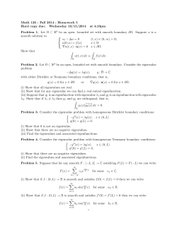
Boundary Tension Between Coexisting Phases of a Block
Article
pubs.acs.org/Macromolecules
Boundary Tension Between Coexisting Phases of a Block Copolymer
Blend
Russell K. W. Spencer and Mark W. Matsen*
Department of Chemical Engineering, Department of Physics & Astronomy, and the Waterloo Institute for Nanotechnology,
University of Waterloo, Waterloo, Ontario, Canada
ABSTRACT: Self-consistent field theory (SCFT) is used to evaluate
the excess free energy per unit area (i.e., tension) of different
boundaries (or interfaces) between the coexisting phases of a block
copolymer blend. In this first study of its kind, we focus on the
boundaries separating the short- and long-period lamellar phases that
form in mixtures of small and large symmetric diblock copolymers of
polymerizations Ns and Nl, respectively, when Ns ≪ Nl. According to
strong-segregation theory (SST), the tension is minimized when both
sets of lamellae orient parallel to the boundary, but experiments
[Hashimoto, et al., Macromolecules 1994, 27, 1562] tend to observe
kink boundaries instead, where the domains of one lamellar phase
evolve continuously into those of the other lamellar phase. Our more
refined SCFT calculations, on the other hand, do predict a lower
tension for the kink boundary consistent with the experimental observations. For completeness, we also examine the boundaries
that form when the short-period lamellar phase disorders, and again the SCFT results are in agreement with experiment.
■
INTRODUCTION
Block copolymers are being used in an expanding range of
applications,1 often in the form of blends2,3 for the simple
reason that their morphology (or microstructure) is more easily
controlled by adjusting a blend ratio than changing molecular
parameters,4,5 which requires synthesizing new molecules.
While neat block copolymer materials typically form polycrystalline morphologies consisting of regions (or grains) with
different orientations of the same ordered phase,6 blends can
also involve regions (or macrodomains) of different ordered
phases. In both cases, the size and shape of the coherent
regions are affected not only by how the material is prepared
(e.g., annealing time, annealing temperature, use of solvent,
etc.), but also by the tension along their boundaries.7 As for
simple uniform phases, a higher boundary tension leads to
larger regions. However, when the phases possess microstructure, then the tension depends upon the relative
orientations between the boundary and the phases, and this
affects the shape of the regions.
There have been several theoretical studies on the grain
boundaries in neat diblock copolymer melts.8−10 Even though
they have focused on the simple lamellar phase, the behavior
has proven to be extraordinarily rich. However, there have yet
to be any analogous studies for blends, where the boundaries
separate different coexisting phases. Admittedly, there are some
studies of the boundaries between different ordered phases of a
neat diblock copolymer melt,11−13 but this is a dynamical
problem as one phase is always more stable than the other
causing the boundary to propagate. On the other hand, a blend
can exhibit coexisting phases resulting in stable boundaries, like
the grain boundaries of a neat melt. The added complication,
© 2015 American Chemical Society
though, is that a blend involves a number of distinct molecular
species, which is the challenge we will address in this paper.
In the interest of starting off with the simplest system
possible, we consider a blend of small and large symmetric AB
diblock copolymers. This system has, in fact, proven to be
particularly intriguing. Calculations14 using strong-stretching
theory (SST)15 initially predicted that such blends would never
macrophase separate under any condition. Shortly after,
however, experiments by Hashimoto et al.16,17 observed
coexisting short- and long-period lamellar (LAM) phases,
when the size ratio of the two diblocks exceeded 1:10. This
contradiction was soon resolved with more accurate calculations,18 using self-consistent field theory (SCFT),19 where the
predicted phase diagrams (see Figure 1) exhibited the
macrophase separation seen in the experiments. This success
was then eclipsed by subsequent experiments,20 which
demonstrated stunning quantitative agreement with the
SCFT predictions.
In addition to the macrophase separation, Hashimoto et al.17
also documented a number of distinct boundaries between the
coexisting LAM phases. The most common was a kink
boundary, where the A- and B-rich domains of the two LAM
phases remain connected through the boundary. In its most
general form depicted in Figure 2a, the short- and long-period
LAM phases are oriented at angles θ(s) and θ(l) to the boundary,
respectively. For the domains to match up, the angles must
satisfy
Received: February 25, 2015
Revised: April 6, 2015
Published: April 16, 2015
2840
DOI: 10.1021/acs.macromol.5b00411
Macromolecules 2015, 48, 2840−2848
Article
Macromolecules
even been observed. Another puzzling result occurs when the
short-period LAM phase disorders. Assuming the remaining
LAM phase is well ordered, SST suggests that its lamellae
would select one of two equally preferred orientations, either
parallel or perpendicular to the boundary.21 While experiments16,17 observe the perpendicular version of the LAM + DIS
boundary, there has been no sign of the parallel orientation.
The failure of SST to account for the experimental
observations may be because the selection of boundaries has
more to do with the kinetics of macrophase separation than the
boundary tension. Alternatively, it could just be that SST does
not provide a sufficiently accurate treatment of the boundaries,
as was the case for the macrophase separation itself. To shed
some light on this, we now compare the different boundaries
using the more refined SCFT.
Figure 1. Phase diagram for blends of small and large symmetric AB
diblock copolymers18 plotted in terms of their size ratio, α = Ns/Nl,
and the volume fraction of small diblocks, ϕ̅ s. The segregation strength
of the large diblocks is fixed at χ Nl = 200. The dot denotes a critical
point, below which the blend separates into coexisting short- and longperiod lamellar (LAM) phases, and the dotted line is an order−
disorder transition (ODT), below which the short-period LAM phase
switches to a disordered (DIS) phase.
■
THEORY
This section describes the self-consistent field theory (SCFT)
for the coexisting phases of a binary blend consisting of ns small
AB diblock copolymers of polymerization Ns and nl large AB
diblock copolymers of polymerization Nl. Here the polymerization of the large diblock, Nl, is chosen as our reference, and
the relative size of the small diblock is specified by α ≡ Ns/Nl.
In this particular study, all diblocks have a symmetric
composition with an equal number of A- and B-type segments.
As usual, we assume an incompressible melt, where each
segment occupies a volume of ρ0−1 and where the A and B
segments are conformationally symmetric with a common
segment length of a. The incompressibility implies that the
volume of our system is fixed at V = (nsNs + nl Nl) /ρ0. The
interaction between the unlike segments is controlled by the
standard Flory−Huggins χ parameter.
The difference between the boundaries in a blend and the
grain boundaries in a neat melt is that each molecular species of
the blend will exhibit either an excess or depletion at a
boundary. Although these excesses (or depletions) will adjust
automatically in the grand-canonical ensemble,22 this ensemble
also allows the position of the boundary to move freely, which
compromises the numerical stability of the calculation.
Consequently, we are forced to use the canonical ensemble,
where the position of the boundary is constrained by the blend
composition.
In the canonical ensemble, the A- and B-segment
concentrations, ϕγ,A(r) and ϕγ,B(r), and the single-chain
partition function, Qγ, are calculated for short and long
diblocks (i.e., γ = s and l, respectively) using the same
expressions as for neat diblocks.23 We solve the necessary
diffusion equations for this part of the calculation using the
pseudospectral algorithm developed by Ranjan et al.24 Of
course, to properly fill the volume V, the concentrations of the
small and large diblocks must be scaled by factors of ϕ̅ s and (1−
ϕ̅ s), respectively, where ϕ̅ s ≡ nsNs/ρ0V is the composition of the
blend. The next step is to adjust the fields acting on the A and
B segments to satisfy the self-consistent conditions,
Figure 2. (a) Kink boundary between the short- and long-period LAM
phases. The continuity of the A- and B-rich domains requires the
lamellar orientations, θ(s) and θ(l), and periods, D(s) and D(l), to satisfy
eq 1. (b) One-sided inclination version of the kink boundary observed
in experiment.17 (c) Parallel boundary favored by SST.
D(s)
cos(θ (s))
=
D(l)
cos(θ (l))
(1)
where D(s) and D(l) are the bulk periods of the respective
phases. Although this avoids creating any excess A/B interface,
the boundary cuts diagonally through the lamellae. In SST,
where the diblock copolymers extend normal to the A/B
interface, this forces the polymers to rearrange the way they fill
space. To minimize the resulting free energy cost, the system
will reduce the kink angle as much as possible. The best it can
do is orient the large lamellae perpendicular to the boundary
(i.e., θ(l) = 0) as depicted in Figure 2b, which in turn minimizes
θ(s). Indeed, this one-sided inclination version of the kink
boundary is exactly what experiments typically observe.17
Although this all seems very reasonable, simple SST-based
reasoning would suggest that the most favorable boundary is
the parallel version depicted in Figure 2c, where both sets of
lamellae are oriented parallel to the boundary (i.e., θ(s) = θ(l) =
90°). According to SST, the tension of such a boundary would
be exactly zero, and thus it is rather perplexing that it has not
wA(r) = χNlϕB(r) + ξ(r)
(2)
wB(r) = χNlϕA (r) + ξ(r)
(3)
where ϕδ(r) ≡ ϕs,δ(r) + ϕl,δ(r) for δ = A or B and ξ(r) is the
pressure field used to enforce the incompressibility condition,
ϕA(r) + ϕB(r) = 1. This is done using an Anderson mixing
scheme devised earlier.25 Once the field equations are satisfied,
the free energy of the system is evaluated using
2841
DOI: 10.1021/acs.macromol.5b00411
Macromolecules 2015, 48, 2840−2848
Article
Macromolecules
⎛ 1 − ϕ̅ ⎞
ϕ̅ ⎛ ϕ̅ ⎞
FNl
s
⎟⎟ + s ln⎜⎜ s ⎟⎟
= (1 − ϕs ̅ ) ln⎜⎜
kBTρ0 V
α ⎝Qs ⎠
⎝ Ql ⎠
+
1
V
∫ [χNlϕA(r)ϕB(r) − wA(r)ϕA(r) − wB(r)ϕB(r)] dr
(4)
Before considering the phase boundary, it is necessary to first
calculate the free energy, F, and period, D, of the bulk LAM
phase as a function of the blend composition, ϕ̅ s, at fixed α.
Figure 3 shows a sample calculation for α = 0.06. From the
Figure 4. System boxes for the (a) parallel and (b) kink boundaries.
The former boundary (at x = xb) just involves a 1D calculation using
reflecting BC’s (at x = 0 and L). However, the later case requires a 2D
calculation with two boundaries (at x = xb1 and xb2) using reflecting
BC’s in the x-direction (at x = 0 and L) and periodic BC’s in the ydirection (at y = 0 and D(l)).
⎛ (F − F )N
ΓbNl1/2
L ⎞
tan
l
⎟⎟
= min⎜⎜
×
L , ϕs ⎝ kBTρ V
kBTρ0 a
aNl1/2 ⎠
0
(5)
To equilibrate the system requires minimization with respect to
L, which allows the lamellae to relax to their preferred
thicknesses, and with respect to ϕ̅ s, which optimizes the excess
(or depletion) of small diblock at the boundary.
Figure 4b displays an appropriate system box for the kink
boundary. In this case, the box contains two boundaries at x =
xb1 and xb2 with the short-period LAM phase between and longperiod LAM phases to either side. As before, initial guesses for
wδ(r) are constructed from the bulk solutions and the
composition is set to ϕ̅ s = [(L + xb1 − xb2)ϕ̅ (l)
s + (xb2 −
xb1)ϕ̅ (s)
s ]/L. Periodic BC’s are applied in the y-direction, which
forces the boundaries to orient perpendicular to the x-direction.
Setting the box size in the y-direction to D(l) forces the longperiod LAM phase to orient with θ(l) = 0, which allows us to
apply reflecting BC’s in the x-direction. For this particular set
up, the boundary tension is given by
ΓbNl1/2
(F − Ftan)Nl
1
L
= ×
×
kBTρ0 a
2
kBTρ0 V
aNl1/2
Figure 3. (a) Free energy, F, and (b) period, D, of a LAM phase
plotted versus the blend composition, ϕ̅ s, for χ Nl = 200 and α = 0.06.
The dots denote the binodal points determined by the double-tangent
line, Ftan, in the upper plot.
(6)
where the factor of one-half accounts for the fact that the
system box contains two boundaries. Because the long-period
lamellae can vary their length to fit the box, there is no need to
minimize Γb with respect to L. Although the system still needs
to adjust the excess (or depletion) of short diblock at the two
boundaries, this does not actually require a minimization with
respect to ϕ̅ s. The system does this automatically by changing
the relative volumes of the two coexisting phases, which is
made possible by the fact that the two long-period LAM
regions can shift in the y-direction independently of each other.
We follow analogous procedures when the short-period LAM
phase disorders producing LAM+DIS coexistence, but there are
a couple of simplifications. For the parallel boundary, the
minimization in eq 5 only needs to be done with respect to
either L or ϕ̅ s, but not both. For the perpendicular case, we
reduce the size of the system box so that it just contains one
boundary, in which case the factor of a half is dropped from eq
6.
double tangent, Ftan, denoted by the dashed line in Figure 3a,
(γ)
we obtain the compositions, ϕ̅ (γ)
s , and periods, D , of the
coexisting phases (γ = s and l) indicated by dots in Figure 3.
With that information in hand, we then choose a system box
with appropriate boundary conditions (BC’s) for the diffusion
equations and construct initial guesses for the fields, wδ(r).
Figure 4a shows a suitable system box for the parallel LAM +
LAM boundary. Given that there is no variation in the lateral
direction, the diffusion equations just have to be solved in one
dimension (i.e., 0 ≤ x ≤ L). This is done with reflecting BC’s,
which constrains the center of a lamellar domain to each end of
the box, x = 0 and L. Of course, the box has to be large enough
that the lamellae at the ends acquire bulk characteristics; we
always repeat our calculations for a range of L values so as to
ensure that our results are free of any noticeable finite-size
effects. To construct initial guesses for wδ(r), we simply splice
the bulk solutions together with a boundary at an x=xb near the
middle of the box. The blend composition is set to ϕ̅ s = [xb ϕ̅ (l)
s
+ (L−xb)ϕ̅ (s)
s ]/L. The field eqs 2 and 3 are then solved, and the
boundary tension, Γb, is obtained from the free energy excess
per unit area,
■
RESULTS
The SCFT is now applied to boundaries corresponding to the
coexistence regions in Figure 1, where the level of segregation
for the large diblock copolymer is fixed at χ Nl = 200 while the
2842
DOI: 10.1021/acs.macromol.5b00411
Macromolecules 2015, 48, 2840−2848
Article
Macromolecules
less segregated. However, the width of the boundary diverges as
the critical point is approached (i.e., α → α−c ). To gauge the
width of the boundary in Figure 5b for α = 0.16, Figure 6 plots
level of segregation for the small diblock copolymer varies as
χ Ns = 200α. The study is broken into three parts. It begins by
examining the morphology of the order−order boundaries,
then that of the order−disorder boundaries, and concludes by
comparing their excess free energies per unit area (i.e.,
tensions).
LAM + LAM Boundaries. We start by examining the
parallel boundary depicted in Figure 2c, where the concentration profiles only depend on x. Figure 5 plots both the total
Figure 6. Average composition of the microdomain layers (dots)
plotted across the parallel LAM + LAM boundary for a blend with α =
0.16. The curve is a fit to eq 7, from which we extract the width of the
boundary, wb. The inset shows a log−log plot demonstrating that wb
diverges at the critical point following a power-law, eq 8, with an
exponent of ν = 1/2.
the average composition, ϕ̅ s, of each microdomain layer as a
function of its position. (Note that the edges of the
microdomains are defined by ϕA(x) =0.5 and the microdomain
positions are defined by their centers.) The width of the
boundary, wb, is then extracted by fitting the points to a
hyperbolic tangent function
ϕs ̅ (x) =
⎛ 2(x − xb) ⎞
1 (s)
(l)
(ϕs̅ − ϕs̅ ) tanh⎜
⎟
2
wb
⎝
⎠
1 (s)
(l)
+ (ϕs̅ + ϕs̅ )
2
Figure 5. Total A concentration, ϕA(x), (solid curves) and total smalldiblock concentration, ϕs(x), (dashed curves) plotted across the
parallel LAM + LAM boundary for blends with (a) α = 0.06 and (b) α
= 0.16. The insets show 2D color plots of ϕA(r), analogous to the ones
that we will use to illustrate kink boundaries.
(7)
This symmetric fitting function assumes that ϕ̅ s(x) converges to
(s)
the bulk values, ϕ̅ (l)
s and ϕ̅ s , at the same rate on both sides of
the boundary, but this is a good approximation near the critical
point. The inset in Figure 6 shows a log−log plot of the width,
wb, versus distance from the critical point, |α−αc|, and the
straight-line segment illustrates that the width diverges as a
power-law,
concentration of A segments (solid curves) and the
concentration of the small diblocks (dashed curves) for a
blend with α = 0.06, where the two LAM phases have very
distinct periods, and for α = 0.16, where the coexisting LAM
phases are relatively similar. For the smaller α, the coexistence
is between an essentially pure small-diblock LAM phase at a
weak segregation of χ Ns = 12 and a strongly segregated LAM
phase consisting mostly of large diblocks but also a significant
amount of small diblock concentrated at the A/B interfaces.
The compositions, ϕ̅ (s)
and ϕ̅ (l)
s
s , of the two phases are, of
course, consistent with the binodal curves of the LAM+LAM
region in Figure 1. In Figure 5b, where α is just below the
critical point, both LAM phases are well segregated and contain
substantial amounts of both diblock species.
As evident from the profiles in Figure 5a, the boundary is
relatively sharp for α = 0.06. In fact, the long-period LAM phase
is virtually indistinguishable from the bulk phase within one
period of the boundary. The short-period LAM phase takes a
couple periods to reach its bulk properties, partly because each
period corresponds to a shorter distance and also because it is
wb ∝ |α − αc|−ν
(8)
with a critical exponent of ν = /2. This is the usual mean-field
exponent for boundaries between two coexisting phases,
including the simple boundary between two immiscible
homopolymers.26
Now we move onto the kink boundary depicted in Figure 2b.
In this case, the morphology varies in both the x- and ydirection, and so Figure 7 plots the total A-segment
concentration, ϕA(r), in 2D using a color scale. The distribution
of small diblocks is essentially equivalent to that of the parallel
boundary, and so we do not include an extra plot for ϕs(r). At α
= 0.06, where there is a significant size difference between the
lamellar periods, the thick lamellae possess relatively square
ends, each with a thin lamella emerging from one of their
corners. The lamellae of the short-period phase then develop
ripples in order to keep their domains relatively uniform in
thickness, while accommodating the square ends of the large
lamellae. These ripples fade toward the bulk, but nevertheless
1
2843
DOI: 10.1021/acs.macromol.5b00411
Macromolecules 2015, 48, 2840−2848
Article
Macromolecules
Figure 7. Total A-segment concentration, ϕA(r), plotted across the
kink LAM + LAM boundary for blends with (a) α = 0.06 and (b) α =
0.16. Each image is 3.0 × 3.5 in units of aNl1/2, and the color scale is
shown at the bottom.
they do persist for a considerable distance from the boundary.
We note that these ripples are clearly evident in the
experimental TEM images,17 including the one displayed in
the Abstract graphic.
As the critical point is approached and the two LAM phases
become similar, the kink angle decreases and the width of the
boundary diverges again. As before, we gauge the width by
examining the change in the average blend composition, ϕ̅ s(x),
plotted in Figure 8 for α = 0.16. In this case, we just average
Figure 9. Analogous plots to Figure 5, but for the parallel LAM+DIS
boundary at (a) α = 0.02 and (b) α = 0.05.
blends with α = 0.02 and 0.05. Consistent with the binodal
curves in Figure 1, the DIS phase is nearly pure small diblock.
While the LAM phase is rich in large diblocks, it does contain a
substantial amount of small diblock. The amount also increases
as α decreases, because smaller molecules gain more translational entropy per unit volume by penetrating into the LAM
phase. Although the small diblocks still accumulate at the A/B
interface, for the most part they uniformly dilute the large
diblocks, which then tends to disorder the LAM phase.27 Figure
10 shows the perpendicular LAM + DIS boundary, where the
lamellae are oriented perpendicular to the boundary. We see
that the truncated lamellae have reasonably square ends at
larger α, but that the ends become somewhat rounded at
smaller α.
Figure 8. Analogous plot to Figure 6, but for the kink LAM + LAM
boundary at α = 0.16. In this case, the composition, ϕ̅ s(x), is obtained
by averaging the concentration of small diblock, ϕs(r), parallel to the
boundary. Again the inset shows a power-law divergence in the width
of the boundary, eq 8, but with an exponent of ν = 3/4.
ϕs(r) in the lateral y-direction, which gives a continuous curve
in the x-direction. Near the critical point, ϕ̅ s(x) is virtually
indistinguishable from the hyperbolic tangent function in eq 7,
which we use to extract the width, wb. The log−log plot in the
inset of Figure 8 illustrates a power-law divergence, eq 8, but
this time it occurs with a critical exponent of ν = 3/4 that is
distinctly larger than the usual value of ν = 1/2. The new
exponent, however, is readily accounted for by a simple
analytical calculation described in the Appendix.
LAM + DIS Boundaries. It is interesting to extend our
calculations to the analogous boundaries at smaller α, where the
short-period LAM phase disorders. Figure 9 plots the
concentration of A segments (solid curves) and small diblock
(dashed curve) across the parallel LAM + DIS boundary for
Figure 10. Analogous plots to Figure 7, but for the perpendicular
LAM+DIS boundary at (a) α = 0.02 and (b) α = 0.05.
2844
DOI: 10.1021/acs.macromol.5b00411
Macromolecules 2015, 48, 2840−2848
Article
Macromolecules
As evident in Figures 9b and 10b, the ordered LAM phase
induces short-range order in the DIS phase. This is illustrated
more clearly in Figure 11, where the A-segment concentration,
Figure 12. Tensions of the parallel (dashed curve) and perpendicular/
kink (dashed curve) boundaries versus relative size of the diblocks.
The vertical dotted line denotes the ODT from Figure 1, and the
insets demonstrate a power-law dependence near the critical point, eq
12, with exponents μ = 3/2 and 5/4, respectively.
Figure 11. Total A-segment concentration, ϕA(r), plotted from the
boundary into the DIS phase for α = 0.05. SCFT results for the parallel
and perpendicular boundaries, Figures 9b and 10b, respectively, are
plotted with black curves (indistinguishable on this scale), and the
WST approximation from eq 9 is shown with a red curve.
region (α < αODT). Both results are consistent with what is
most commonly observed in experiment.
The tensions of the parallel LAM + LAM and LAM + DIS
boundaries (Figures 5 and 9, respectively) form a continuous
curve across the ODT (dotted line in Figure 12). This is
because the short-period LAM phase evolves continuously into
the DIS phase on account of the ODT being a second-order
transition. However, it is less obvious that the tensions of the
kink LAM + LAM and perpendicular LAM + DIS boundaries
are continuous across the ODT, because it is not immediately
clear how the morphology of the kink boundary with its
connected short-period lamellae (see Figure 7a) would evolve
smoothly into the perpendicular boundary with its disconnected domains in the DIS phase (see Figure 10b). From
calculations very close to the ODT, it appears that the thin
lamellae begin pinching off starting next to the boundary and
then extending outward as α → α+ODT. In this way, the kink
boundary does transform continuously into the perpendicular
boundary across the ODT.
In the other direction, α → α−c , the tension of both LAM +
LAM boundaries must vanish, since the coexisting LAM phases
become identical at the critical point. As usual for critical
points, the tension should vanish following a power-law,
ϕA(x), in the DIS phase is plotted as a function of distance, x −
xb, from the boundaries. (For the perpendicular boundary, the
profile is plotted along a line extending through the center of an
A-rich lamella.) The profiles from both boundaries are so
similar that they appear indistinguishable on the scale of our
plot, so long as we adjust xb appropriately.
The profiles in Figure 11 are reminiscent of the surface
ordering examined by Fredrickson28 for disordered diblock
copolymer melts next to a preferential surface. Using an
approximation to weak-segregation theory (WST),29 Fredrickson predicted exponentially decaying oscillations,
ϕA (x) = A 0 exp( −x /ζ ) cos(kx + ϕ0)
(9)
where in the case of symmetric molecules (i.e., f = 0.5) the
decay length is given by
⎤−1/2
⎡3
ζ
(10.495
N
)
=
−
χ
⎥⎦
⎢⎣ 2
aN1/2
(10)
Γb ∝ |α − αc| μ
and the wavevector of the oscillation is
⎤1/2
⎡3
kaN1/2 = ⎢ (χN − 10.495 + 8 3 )⎥
⎦
⎣2
(12)
with some critical exponent, μ. The insets in Figure 12 illustrate
that the parallel boundary is consistent with the usual critical
exponent of μ = 3/2,26 while the kink boundary is consistent
with the smaller exponent of μ = 5/4 derived in the Appendix.
Although the difference in μ is not as pronounced as that of ν
for the boundary width in eq 8, the difference is undoubtedly
real because each pair of exponents should satisfy the relation μ
+ ν = 2.30
(11)
Because our disordered phase is nearly pure, we can apply this
prediction with N replaced by Ns. Given that χ Ns = 10 for α =
0.05, it follows that ζ/aNs1/2 = 1.16 and kaNs1/2 = 4.48. The red
curve in Figure 11 is fit to eq 9 using these values of ζ and k
while adjusting A0 and ϕ0. Considering the approximations
involved, this prediction by Fredrickson captures the effect
rather well.
Boundary Tensions. Now that we have finished examining
the morphologies of our candidate boundaries, Figure 12
compares their tensions as a function of α. The comparison
reveals that the kink boundary is preferred over the parallel
boundary in the LAM + LAM region (αODT < α < αc), apart
from a small interval near the critical point where their tensions
are similarly small. Likewise, the perpendicular boundary has a
lower tension than the parallel boundary in the LAM+DIS
■
DISCUSSION
This study is the first to demonstrate the application of SCFT
to boundaries between coexisting ordered phases in a block
copolymer blend. In principle, blends are most easily treated in
the grand-canonical ensemble, where the composition adjusts
automatically, avoiding the need to minimize the excess free
energy with respect to the composition, ϕ̅ s. In this ensemble,
however, it proves difficult to converge the self-consistent field
eqs 2 and 3. We attribute the difficulty to the fact that the
2845
DOI: 10.1021/acs.macromol.5b00411
Macromolecules 2015, 48, 2840−2848
Article
Macromolecules
comparable to the lamellar periods. The only excess that is
unambiguous is that of the total grand-canonical free energy
(i.e., the boundary tension).
We have assumed, based on experimental evidence and some
rational arguments, that the long-period LAM phase is
perpendicular to the boundary (i.e., θ(l) = 0). The tension,
however, might decrease somewhat when the large lamellae are
slightly tilted relative to the boundary. In principle, the SCFT
could be solved with both LAM phases tilted provided we
implemented periodic BC’s in both the x- and y-directions.
However, the long-period phase would have to wrap around the
periodic BC’s in the y-direction at least once, which for small
tilt angles would require a very large system size in the xdirection. Unfortunately this is not computationally feasible.
Alternatively, it may seem conceivable that the semianalytical
calculation in the Appendix could address this issue. However,
that calculation is only valid near the critical point where the
two phases are nearly identical. In this limit, the tension
becomes insensitive to the orientation of the boundary, and
unfortunately this results in very small energy variations which
the analytical treatment is not sufficiently accurate to resolve.
While the experiments16 reported evidence of macrophase
separation when the size ratio exceeded 1:5 (i.e., α ≲ 0.2), they
only observed LAM + LAM coexistent for size disparities
beyond about 1:10 (i.e., α ≲ 0.1). This is readily explained by
our prediction that the boundary tension vanishes and the
boundary width diverges as the critical point is approached.
The lower tensions will result in smaller bulk regions and the
increased width will make the regions less discernible. Thus, if
the experiments are not sufficiently far from the critical point,
they will likely just observe what appears to be a poorly ordered
LAM phase consisting of wavy lamellae with a fluctuating
domain thickness.
While the kink boundary has a lower tension than the parallel
boundary, the energies are not hugely different. We would still
expect to observe the occasional parallel boundary, but there is
no evidence of any in the published TEM images.16,17 Perhaps
the solvent-casting process used to create the experimental
samples enhances the preference for the kink boundary. Indeed,
solvent should reduce the packing frustration,36 responsible for
the ripples in the thin lamellae. Another potential explanation is
that the formation of kink boundaries may have a kinetic
advantage. The macrophase separation of the small and large
diblocks requires the macroscopic transport of material, and it
is understood that the flow of block copolymers happens more
easily parallel to the lamellae.37 Naturally, the boundary would
tend to form perpendicular to the flow direction, thus resulting
in a further preference for the kink boundary.
There are many directions that future work could take. For
instance, it would be useful to investigate how added solvent
(or homopolymer) affects the boundaries, as this could very
well shed further light on the strong preference for the kink
boundary in the experiments of Hashimoto et al.17 Their
experiments also documented other LAM + LAM boundaries,
which would be interesting to examine. Furthermore, our
calculations could be extended to boundaries between ordered
phases of different symmetries, such as lamellar and
cylindrical,38−40 not to mention all the other potential phase
combinations exhibited by block copolymer blends.
relative amounts of the coexisting phases are free to vary, which
allows the boundary to drift. Furthermore, any inaccuracy in the
chemical potential exacerbates the problem, in that it gives one
phase a slight preference over the other, causing it to consume
the entire system box. In the canonical ensemble, on the other
hand, the relative amounts of the two phases are constrained by
the fix composition, ϕ̅ s. In some cases, it is not even necessary
to minimize Γb with respect to ϕ̅ s, but even if it is, the extra
computational cost is minimal and certainly worth the added
numerical stability. In reality, the most important consideration
in regards to numerical cost is finding the smallest possible
system box with appropriate boundary conditions (BC’s) in
which to solve the diffusion equations of SCFT.
SCFT continues to build up an impressive track-record in
regards to blends of small and large symmetric diblock
copolymers, particularly in comparison to SST. First, the
SCFT prediction for the distribution of small and large diblocks
within a LAM phase is in good agreement with experiment,31
far more so than that of SST.32,33 Second, SCFT predicts the
LAM+LAM and LAM+DIS coexistence18 with amazing
accuracy,20 whereas SST fails to even anticipate the macrophase
separation.14 Now we see that SCFT favors the kink boundary
observed in experiments17 over the parallel boundary favored
by SST.
Although SST is not expected to be quantitatively accurate, it
has a reputation for providing reliable qualitative explanations
for phase behavior.34 In the strong-segregation limit, the free
energy of the individual monolayers of the lamellar phase are
independent of each other, and thus there is no energetic
penalty for placing a thin monolayer next to a thicker
monolayer, which is why SST predicts zero tension for the
parallel boundary. On the other hand, there is an energetic cost
to truncating a monolayer at an angle to the lamellar normal
(i.e., θ(γ) ≠ 0). In the SST, the polymer chains extend
perpendicular to the A/B interface, and thus a nonzero θ(γ)
requires the rearrangement of chain trajectories, which in turn
causes packing frustration.23 Although this is avoided in the
long-period phase by having θ(l) = 0, the short-period phase still
requires θ(s) > 0 in order to maintain the continuity of the
domains. Thus, the packing frustration cannot be completely
eliminated, and so SST will necessarily predict a positive
tension for the kink boundary. Although the relative stability of
the parallel and kink boundaries is opposite to what our SCFT
calculation predicts, it is known that SCFT converges to SST in
limit of χ → ∞,35 and so our SCFT prediction must eventually
reverse at sufficiently high segregation.
There is no simple explanation of why SCFT predicts a lower
tension for the kink boundary than the parallel boundary. After
all, qualitative explanations for block copolymer phase behavior
are generally based upon the SST description. The fact that
SCFT predicts the opposite to SST implies that the explanation
is a subtle one related to the finite segregation of the melt. It
may seem plausible that an explanation could be found by
decomposing the excess free energy of the boundaries into
various contributions, such as enthalpy, stretching energies of
the blocks, and translational entropy of the junction points.34
While such excesses are well-defined for a grain boundary
between the same phase, they are not for boundaries between
different phases. In the later case, where the free energy
contributions have different values in the neighboring phases,
the excesses depend on how one defines the position of the
boundary, xb. Unfortunately, there is no definitive definition of
xb, particularly when the width of the boundary, wb, is
■
SUMMARY
Self-consistent field theory (SCFT) has been used to examine
boundaries (or interfaces) between coexisting lamellar (LAM)
2846
DOI: 10.1021/acs.macromol.5b00411
Macromolecules 2015, 48, 2840−2848
Article
Macromolecules
coefficient, κ, throughout the boundary; this becomes a good
approximation near the critical point where the two coexisting
phases are very similar. The second term is the compression
energy, U(D) = F − Ftan, obtained from a calculation like that of
Figure 3.
The equilibrium solution for θ(x) is determined by
minimizing eq 13 using calculus of variations. The minimum
corresponds to the Euler-Lagrange equation, which can be
integrated to give
phases in blends of small and large symmetric diblock
copolymers. The calculations were performed specifically for
the phase diagram in Figure 1, where the segregation strength
of the large diblock was fixed at χNl = 200 while the relative size
of the small diblock was controlled by α = Ns/Nl. In particular,
we compared the kink boundary (Figure 2b) most commonly
observed in experiments16,17 with the parallel boundary (Figure
2c) suggested by strong-stretching theory (SST). Contrary to
SST, the SCFT predicted a lower tension, Γb, for the kink
boundary consistent with the experimental observations.
Furthermore, the predicted morphology nicely agrees with
the experimental TEM images in that the ends of the large
lamellae induced long-range ripples in the thin lamellae. We
also found that, as the critical point is approached, the width of
the boundary diverges and the tension vanishes. This may
explain why the experiments required a size ratio between the
diblocks of at least 1:10 to observe LAM + LAM coexistent,
while SCFT predicts that 1:5 is sufficient to cause macrophase
separation.
For completeness, we also examined the boundaries at small
α, where the short-period LAM phase disorders producing
LAM + DIS coexistence. In this case, the tension is lower when
the lamellae of the remaining LAM phase are oriented
perpendicular to the boundary than when they are parallel.
Again this is consistent with what is observed in experiment.
Interestingly, the LAM phase induces long-range composition
oscillations in the DIS phase, which are well described by a
prediction28 from weak-segregation theory (WST).
This study has provided the first application of SCFT to the
boundaries between coexisting phases of a block copolymer
blend. The key to the calculation was identifying a finite system
box with appropriate boundary conditions (BC’s) in which to
solve the modified diffusion equations of SCFT. Converging
the self-consistent field conditions was also a nontrivial task,
particularly because our system had a weak tendency to
macrophase separate. Although the grand-canonical ensemble is
the natural choice for blends, we had to perform our calculation
in the canonical ensemble in order to prevent the boundary
from drifting. Depending on the details of the boundary, the
calculation may or may not require minimization of the tension
with respect to the box size and/or blend composition. The
treatment of each boundary has to be considered on an
individual basis. Hopefully, our examples will open the door to
future studies on the multitude of interesting boundaries
exhibited by block copolymer blends.
κ ⎛⎜ dθ ⎞⎟
− U (D) = constant
2 ⎝ dx ⎠
2
The resulting constant of integration needs to be set to zero so
that θ(x) converges to a constant in each of the two bulk
regions, where U(D(γ)) = 0 for γ = s and l. With that
simplification, it follows that the minimization requires
dθ
=
dx
∫
(17)
where Dc is the equilibrium lamellar period at the critical point.
The critical point occurs when the coefficient of the quadratic
term switches sign causing the single minimum at Dc to
bifurcate into two minimums at
D(γ ) = Dc ±
B|α − αc|
2C
(18)
where γ = s and l correspond to the minus and plus signs,
respectively. As usual in these type of Landau calculations, the
coefficient of the quadratic term is taken to be linear in the
control parameter α, while ignoring any α-dependence in the
coefficient of the quartic term. Given that, we require the
constant term to be
A=
B2 (α − αc)2
4C
(19)
so as to satisfy U(D(γ)) = 0.
The width of the boundary will be proportional to the total
change in θ(x) divided by the maximum rate of change, which
occurs at D = Dc. Therefore, it follows that
wb ∝
θ (s) − θ (l)
( ddθx )
∝
max
θ (s)
A
(20)
(s)
From eq 14, we have the relation, D = D cos(θ(s)).
Substituting the bulk periods from eq 18 and expanding the
cosine function for small angles gives θ(s) ∝ |α − αc|1/4.
Inserting this along with eq 19 into our previous expression for
the width, it follows that
wb ∝ |α − αc|−3/4
∞
(l)
(21)
To obtain a similar scaling relation for Γb, we note that eq 16
allows us to express eq 13 as an integral of 2U(D). Thus, the
tension, Γb, will be proportional to the peak value of U(D) (i.e.,
A) times the width of the boundary (i.e., wb), which
immediately implies that
(13)
where the local lamellar period, D, is related to the tilt angle by
D = D(l) cos(θ)
(16)
U (D) ≈ A + B(α − αc)(D − Dc )2 + C(D − Dc )4
■
⎡ κ ⎛ dθ ⎞ 2
⎤
⎢ ⎜ ⎟ + U (D)⎥ dx
−∞ ⎣ 2 ⎝ dx ⎠
⎦
2U (D)/κ
Near the critical point, the compression energy can be
expanded as
APPENDIX
Here we perform a simple analytical calculation to understand
how the kink LAM + LAM boundary behaves as the critical
point is approach (i.e., α → α−c ). In this regime, the tilt angle,
θ(x), between the lamellar normal and the y-axis varies slowly
from θ(l) = 0 to θ(s) > 0 as x increases (see Figure 2). Given that
θ(x) is slowly varying (see Figure 7b), we can then express the
tension of the boundary as8
Γb ∝
(15)
(14)
The first contribution in eq 13 comes from the bending energy
of the lamellae, for which we assume a constant bending
Γb ∝ |α − αc|5/4
2847
(22)
DOI: 10.1021/acs.macromol.5b00411
Macromolecules 2015, 48, 2840−2848
Article
Macromolecules
■
(34) Matsen, M. W.; Bates, F. S. J. Chem. Phys. 1997, 106, 2436−
2448.
(35) Matsen, M. W. Eur. Phys. J. E 2010, 33, 297−306.
(36) Matsen, M. W.; Bates, F. S. Macromolecules 1996, 29, 7641−
7644.
(37) Lodge, T. P.; Dalvi, M. C. Phys. Rev. Lett. 1995, 75, 657−661.
(38) Yamaguchi, D.; Shiratake, S.; Hashimoto, T. Macromolecules
2000, 33, 8258−8268.
(39) Yamaguchi, D.; Hashimoto, T. Macromolecules 2001, 34, 6495−
6505.
(40) Yamaguchi, D.; Hasegawa, H.; Hashimoto, T. Macromolecules
2001, 34, 6506−6518.
AUTHOR INFORMATION
Corresponding Author
*(M.W.M.) E-mail: [email protected].
Notes
The authors declare no competing financial interest.
■
ACKNOWLEDGMENTS
This work was supported with start-up funds from the
University of Waterloo and with computer resources from
SHARCNET.
■
REFERENCES
(1) Bates, F. S.; Fredrickson, G. H. Phys. Today 1999, 52, 32−38.
(2) Abetz, V.; Goldacker, T. Macromol. Rapid Commun. 2000, 21,
16−34.
(3) Ruzette, A.-V.; Leibler, L. Nat. Mater. 2005, 4, 19−31.
(4) Matsen, M. W.; Bates, F. S. Macromolecules 1995, 28, 7298−7300.
(5) Wu, Z.; Li, B.; Jin, Q.; Ding, D.; Shi, A.-C. Macromolecules 2011,
44, 1680−1964.
(6) Ryu, H. J.; Fortner, D. B.; Rohrer, G. S.; Bockstaller, M. R. Phys.
Rev. Lett. 2012, 108, 107801.
(7) Ryu, H. J.; Fortner, D. B.; Lee, S.; Ferebee, R.; de Graef, M.;
Misichronis, K.; Averopoulos, A.; Bockstaller, M. R. Macromolecules
2013, 46, 204−215.
(8) Matsen, M. W. J. Chem. Phys. 1997, 107, 8110−8118.
(9) Duque, D.; Schick, M. J. Chem. Phys. 2000, 113, 5525−5530.
(10) Duque, D.; Schick, M. J. Chem. Phys. 2002, 117, 10315−10320.
(11) Goveas, J. L.; Milner, S. T. Macromolecules 1997, 30, 2605−
2612.
(12) Wickham, R. A.; Shi, A.-C.; Wang, Z.-G. J. Chem. Phys. 2003,
118, 10293−10305.
(13) Spencer, R. K. W.; Wickham, R. A. Soft Matter 2013, 9, 3373−
3382.
(14) Zhulina, E. B.; Birshtein, T. M. Polymer 1991, 32, 1299−1308.
(15) Semenov, A. N. Sov. Phys. JETP 1985, 61, 733−742.
(16) Hashimoto, T.; Yamasaki, K.; Koizumi, S.; Hasegawa, H.
Macromolecules 1993, 26, 2895−2904.
(17) Hashimoto, T.; Koizumi, S.; Hasegawa, H. Macromolecules 1994,
27, 1562−1570.
(18) Matsen, M. W. J. Chem. Phys. 1995, 103, 3268−3271.
(19) Helfand, E. J. Chem. Phys. 1975, 62, 999−1005.
(20) Papadakis, C. M.; Mortensen, K.; Posselt, D. Eur. Phys. J. B
1998, 4, 325−332.
(21) According to SST, the enthalpic cost of the LAM + DIS
boundary is insensitive to the orientation of the LAM phase, and so
the preferred boundaries are the two that do not perturb the chain
trajectories in the LAM phase.
(22) Matsen, M. W. Phys. Rev. Lett. 1995, 74, 4225−4228.
(23) Matsen, M. W. J. Phys.: Condens. Matter 2002, 14, R21−R47.
(24) Ranjan, A.; Qin, J.; Morse, D. C. Macromolecules 2008, 41, 942−
954.
(25) Matsen, M. W. Eur. Phys. J. E 2009, 30, 361−369.
(26) Binder, K. Acta Polym. 1995, 46, 204−225.
(27) Naughton, J. R.; Matsen, M. W. Macromolecules 2002, 35,
5688−5696.
(28) Fredrickson, G. H. Macromolecules 1987, 20, 2535−2542.
(29) Leibler, L. Macromolecules 1980, 13, 1602−1617.
(30) The relationship between exponents occurs because the
boundary tension is proportional to the width of the boundary
times the height of the energy barrier separating the coexisting phases,
which is proportional to |α − αc|2.
(31) Koneripalli, N.; Levicky, R.; Bates, F. S.; Matsen, M. W.; Satija,
S. K.; Ankner, J.; Kaiser, H. Macromolecules 1998, 31, 3498−3508.
(32) Milner, S. T.; Witten, T. A.; Cates, M. E. Macromolecules 1989,
22, 853−861.
(33) Birshtein, T. M.; Liatskaya, Y. V.; Zhulina, E. B. Polymer 1990,
31, 2185−2196.
2848
DOI: 10.1021/acs.macromol.5b00411
Macromolecules 2015, 48, 2840−2848


© Copyright 2026