1. science
2. mathematics
3. geometry

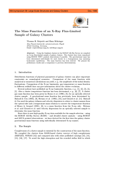
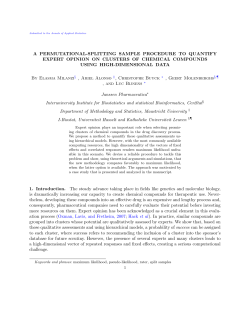
Finding Strongly-Knit Clusters in Social
Networks
Nina Mishra 1
Search Labs, Microsoft Research
Robert Schreiber
HP Labs
Isabelle Stanton ∗,2
Department of Computer Science, University of California, Berkeley
Robert E. Tarjan
Department of Computer Science, Princeton University and HP Labs
Abstract
Social networks are ubiquitous. The discovery of close-knit clusters in these networks
is of fundamental and practical interest. Existing clustering criteria are limited in
that clusters typically do not overlap, all vertices are clustered and/or external
sparsity is ignored. We introduce a new criterion that overcomes these limitations
by combining internal density with external sparsity in a natural way.
This paper explores combinatorial properties of internally dense and externally
sparse clusters. A simple algorithm is given for provably finding such clusters assuming a sufficiently large gap between internal density and external sparsity. Experiments show that the algorithm is able to identify over 90% of the clusters in
real graphs, assuming conditions on external sparsity.
Key words: graph clustering, overlapping clusters, social networks,
Internet Mathematics
2 November 2009
1
Introduction
Social networks have gained in popularity recently with the advent of sites such as
Facebook, Orkut, etc. The number of users participating in these networks is large,
e.g., hundreds of millions in Facebook, and growing. These networks are becoming
a rich source of data as users populate their profiles with personal information. Of
particular interest in this paper is the graph structure induced by the friendship links.
A fundamental problem related to these networks is the discovery of clusters or communities. Intuitively, a cluster is a collection of individuals with dense friendship
patterns internally and sparse friendships externally. There are many reasons to seek
tightly-knit communities in networks, for instance, target marketing schemes can be
designed based on clusters.
What defines a cluster in a social network? At first glance, the answer would seem
to be identical to a traditional cluster in a graph. However, it turns out that the
notions are quite different. The reason stems from some of the initial motivations
for studying graph clustering: to partition a large graph into multiple processors so
that inter-processor communication is minimized and load is approximately balanced.
In a multi-processing environment, each vertex of the graph is assigned to exactly
one cluster and the number of vertices assigned to each processor is approximately
the same. The number of edges crossing the cut is an important component of the
optimization. This criteria does not apply to a social network: a person can belong
to multiple clusters, not every person needs to be clustered, clusters can contain a
varying number of members. Further, internal density of a cluster matters, the number
of edges crossing between two clusters may be quite large, but any person outside of
a cluster should have little adjacency into the cluster.
Closer to our work is the notion of a community which has been considered in prior
work. A subset of vertices is said to form a community [6] if each vertex has at least
as many edges into the community as outside the community. One problem with such
a definition is that individuals with high degree will ultimately not belong to any
community. Such highly-connected individuals are crucial to understanding network
∗ Corresponding Author.
Email addresses: [email protected] (Nina Mishra), [email protected]
(Robert Schreiber), [email protected] (Isabelle Stanton),
[email protected] (Robert E. Tarjan).
1 Work done while at the University of Virginia
2 Supported by a National Physical Science Consortium Fellowship and a Google Anita
Borg Scholarship
2
structure. While this definition is closer to what we seek, it is still missing many
important components: external sparsity, overlapping clusters where not every vertex
is clustered and internal density.
In this paper, we formulate a new graph clustering criterion that is ideally suited
for social networks. We consider an induced subgraph to be a cluster if its internal
density is sufficiently large (β) and if vertices outside the cluster have sufficiently
sparse connectivity into the cluster (α). Specifically, a subset of vertices forms an
(α, β)-cluster if every vertex in the cluster is adjacent to at least a β-fraction of the
cluster and every vertex outside of the cluster is adjacent to at most an α-fraction
of the cluster (Definition 3). Our analysis provides a rigorous understanding of the
combinatorics of (α, β)-clusters, together with a provable algorithm for finding them.
The (α, β)-criterion allows clusters to overlap and does not necessarily cluster every
vertex.
1.1 Contributions
Clusters in social networks take on different characteristics, i.e., overlapping, internally dense and externally sparse. We give a novel formulation, (α, β)-clustering,
specifically suited to these networks.
We investigate combinatorial properties of (α, β)-clusters. We bound the extent to
which two clusters can overlap. For two clusters of equal size, we show that they
overlap in at most (1 − (β − α)) fraction of the vertices. For certain values of α and β,
it is possible for one cluster to be contained in another. We show that if the ratio of
the size of the largest cluster to the smallest cluster is at most 1−α
then one cluster
1−β
cannot be contained in another.
Finally,
we give a loose upper bound on the number
n
s
of (α, 1)-clusters of size s, αs+1
/ αs+1
, where n is the number of vertices.
Next, we introduce the notion of a ρ-champion of a cluster: a vertex in the cluster
with a bounded number of neighbors outside of the cluster, specifically no more than
a ρ fraction of C. If ρ is less than β then intuitively the champion has more neighbors
inside the cluster than out. We assume that the goal of clustering is to find (α, β)clusters that have at least one ρ-champion.
How can one find such clusters? We show that if there is a large gap between α/2
and β i.e., β > 12 + ρ+α
then there is a deterministic algorithm for finding all clusters
2
that runs in time roughly quadratic in the number of vertices.
To validate our ρ-champion assumption and algorithm, we conduct an experiment
3
that evaluates the effectiveness of the clustering algorithm. We demonstrate that our
clustering algorithm succeeds in finding all (α, 1)-clusters with ρ-champions. We compare the clusters we discover with a ground-truth algorithm for finding all maximal
cliques in a graph. The experiments demonstrate that our algorithm finds over 90%
of the clusters in the graph, assuming conditions on external sparsity. Furthermore,
(α, β)-clusters truly exist in these graphs.
2
Related Work
Our (α, β)-clustering formulation is new but has been considered in restricted settings under different guises. The problem of finding the connected (0, β)-clusters in a
graph can be reduced to first finding connected components and then outputting the
components that are β-connected. This problem can be solved efficiently via depth
first search in O(|E| + |V |) time for a graph G = (V, E). Also, the problem of finding
(1− n1 , 1)-clusters is equivalent to finding the maximal cliques in a graph. This problem
has a rich history. Known algorithms find all maximal cliques in time that depends
polynomially on the size of the graph and the number of maximal cliques [25,15].
The problem of finding ((1 − ǫ)β, β)-clusters, for small ǫ, has also been studied under
the name of finding quasi-cliques. Abello et al. [1] present a method for finding subgraphs with average connectivity β. Hartuv and Shamir [11] find densely connected
subgraphs where β > 1/2 via a min-cut algorithm. In the bipartite case, Mishra et
al. [20] consider the problem of finding dense, well-separated bipartite subgraphs.
These algorithms ignore external sparsity (α). External sparsity turns out to be quite
important: an example in Figure 2 shows that there is only one (1/n, 1−1/2n)-cluster,
but if α is ignored, then there are 2n ( n−1
, 1)-clusters, an undesirable consequence.
n
Spectral clustering is a very popular method that involves recursively splitting the
graph using various criteria, e.g., the principal eigenvector of the adjacency matrix.
Successful approaches have been employed by [16,23,17,24,21], among many others.
All of these approaches do not allow overlapping clusters which is one of the main
goals of our work.
Newman and others have advocated modularity as an optimization criterion for graph
partitioning [21]. The modularity of a partition is the amount by which the number
of edges between vertices in the same subset exceeds the number predicted by the
degree-distribution preserving random graph model of Chung [2]. Newman proposed
several methods for optimizing modularity, among them a spectral approach, and
others have found competitive methods as well.
4
Flake et al. [7] use a recursive cut approach intended to optimize the expansion of
the clustering but use Gomory-Hu trees [9] to find the cut instead of eigenvectors.
The expansion of a cut is very similar to the conductance of a cut. The minimum
quality of the clustering is guaranteed by adding a sink to the graph. Again, the goal
of this work is different from ours in that a partitioning is constructed, disallowing
overlapping clusters.
Modeling flow through a network is another way to cluster a graph [7,5]. MCL models
flow through two alternating Markov processes, expansion and inflation. MCL has
been widely used for clustering in biological networks but requires that the graph be
sparse and only finds overlapping clusters in restricted cases. (α, β)-clustering has no
restrictions on the general structure of the graph and allows clusters of different sizes
to overlap.
There has also been considerable work in finding communities on the web [19,8,4,6,13].
For instance, Kumar et al. [19] approach the problem as one of finding bicliques as the
cores of communities. Dourisboure et al. [14] consider a very similar internal density
community definition. Their methods are able to find clusters in graphs with hundreds
of millions of nodes. A key difference between their work and ours is the notion of
external sparsity.
Finally, there has been previous work finding overlapping clusters. Gregory [10], Palla
et. al. [22] and Zhang et. al. [27] have all developed distinct methods for uncovering
overlapping community structures. For example, [22] defines a community as a series
of connected k-cliques while [27] adapts the modularity definition for use with fuzzy
c-means clustering. While both methods allow overlapping clusters neither considers
our external sparsity criterion.
3
Preliminaries
In this section, we give some notation that will be useful for the rest of the paper and
also formally define the (α, β)-clustering problem.
3.1 Notation
We use the following notation to describe our results. For a graph G = (V, E), n
denotes the number of vertices and m denotes the number of edges. For a subset of
vertices A ⊆ V , |A| denotes the number of vertices in A. E(v, A) denotes the set of
5
0123
7654
89:;
?>=<
g?
c
 ???
??



?


?
?


89:;
?>=<
89:;
?>=<
89:;
?>=<
f
b ??
d
 ???

??


?
? 
? 
0123
7654
0123
7654
e
a
89:;
?>=<
h
0123
7654
i
Fig. 1. Overlapping clusters.
edges between a vertex v and a subset of vertices A. For B ⊆ V , E(A, B) denotes
the set of edges between A and B. The neighbors of a vertex v are denoted by Γ(v).
The vertices that are in a ball of radius r around v are denoted Br (v) and include
vertices that are 1, 2, . . . , r hops from v. Thus, for instance, B2 (v) = Γ(v) ∪ Γ(Γ(v)).
The affinity that a vertex, v, has with a set X is exactly |Γ(v) ∩ X|.
3.2 Formal Definition of (α, β)-clustering
What is a good cluster in a social network? There are numerous existing criteria
for defining good graph clusters, and a multitude of algorithms accompanies each
criterion. One popular criterion is based on finding clusters of high conductance. The
conductance of a cut A, B is the ratio of the number of edges crossing the cut to the
minimum of the volume of A and B, where the volume of A is the number of edges
emanating from the vertices in A. Intuitively, conductance is the fraction of edges
coming out of A that cross the cut. The conductance of a cluster is the minimum
conductance of any cut in the cluster.
A spectral algorithm typically uses the eigenvector of a matrix related to the adjacency
matrix to find a good cut of the graph into subgraphs A, B. The process is then
recursively repeated (on A and B) until k clusters are found (where k is an input
parameter) or until the conductance of the next best cut is larger than some threshold.
Formal guarantees can be proved for some variants of this basic algorithm [16].
Cut-based graph clustering algorithms produce a strict partition of the graph, which
is particularly problematic for social networks, as illustrated in Fig. 1. In this graph,
d belongs to two clusters {a, b, c, d} and {d, e, f, g}. Furthermore, h and i need not
be clustered. A cut-based approach will either put {a, b, c, d, e, f, g} into one cluster,
which is not desirable since e, f, g have no edges to a, b, c, or cut at d, putting d into
one of the clusters, say {a, b, c, d}, but leaving d out of {e, f, g} – which leaves a highly
connected vertex outside of the cluster.
The example in Figure 1 motivates a new formulation of the graph clustering problem
that does not stipulate that each vertex belong to exactly one cluster. Our objective is
6
to identify clusters that are internally dense, i.e., each vertex in the cluster is adjacent
to at least a β-fraction of the cluster, and externally sparse, i.e., any vertex outside
of the cluster is adjacent to at most an α-fraction of the vertices in the cluster.
Definition 1 Given a graph, G = (V, E), where every vertex has a self-loop 3 C ⊂ V
is an (α, β)-cluster if
(1) Internally Dense: ∀v ∈ C, |E(v, C)| ≥ β|C|
(2) Externally Sparse: ∀u ∈ V \ C, |E(u, C)| ≤ α|C|
Given 0 ≤ α < β ≤ 1, the (α, β)-clustering problem is to find all (α, β)-clusters.
The new clustering criterion does not seek a strict partitioning of the data. To see
why clusters can overlap, return to Fig. 1. Both {a, b, c, d} and {d, e, f, g} are ( 14 , 1)clusters. Furthermore, h and i do not fall into an (α, β)-cluster if 0 ≤ α < 12 < β ≤ 1,
and consequently would not be clustered.
Observe that when β → 1, the cluster C approaches a clique, and when α → 0,
an (α, β)-cluster tends to a disconnected component. We want α < β since vertices
outside of a cluster should have fewer neighbors in the cluster than vertices that
belong to the cluster.
4
Combinatorics of (α, β)-clusters
In this section, we discuss several combinatorial properties of (α, β)-clusters including
cluster overlap, containment and number of clusters.
4.1 Cluster Overlap
Given two (α, β)-clusters A, B where |A| ≥ |B|, we now determine the maximum size
of the overlap, namely |A ∩ B|. In the case where β = 1, |A ∩ B| can be no larger than
α|B| (otherwise, there would be a vertex outside of B that is adjacent to more than
α of B). Alternatively, in the case where α = 0, |A ∩ B| must be 0. More generally, we
seek a bound for arbitrary values of α and β. We express the overlap as the fraction
of vertices in A, i.e., γ = |A∩B|
.
|A|
3
This is a technical assumption needed to ensure that β = 1 clusters are possible.
7
Proposition 2 For two (α, β)-clusters, A and B, where |A| ≥ |B| and A 6= B, an
upper bound on γ is 1 − (β − α |B|
).
|A|
PROOF. Let u ∈ A \ B. From the α criterion we know that no element of A \ B is
connected to more than α of B. Formally, α|B| ≥ |E(u, A ∩ B)|. Similarly, |E(u, A ∩
B)| ≥ |A ∩ B| − (1 − β)|A| since u is connected to at least β of A. Combining these
inequalities we get α|B| ≥ |A ∩ B| − (1 − β)|A| and solving for |A ∩ B| we have
|A ∩ B| ≤ (1 − β)|A| + α|B|
γ=
|A∩B|
|A|
so γ ≤ 1 − (β − α |B|
).
|A|
(1)
2
When β = 1, the above bound implies that γ ≤ α |B|
– which is tight. However, if
|A|
we let α = 0, the bound indicates that γ ≤ (1 − β) – which is weak, γ should be 0
since α = 0 implies that each cluster is disconnected from the rest of the graph. We
now prove a bound that is tight in the case that α = 0 and β > 21 . This bound is not
useful when β is close to or less than 21 .
Corollary 3 For two (α, β)-clusters, A and B, where |A| ≥ |B| and β > 21 , an upper
α |B|
bound on the ratio of the intersection, |A ∩ B|, to the larger one, |A|, is γ ≤ 2β−1
|A|
PROOF. Let u ∈ A \ B. From the definition of an (α, β)-cluster we know that
|E(u, A ∩ B)| ≤ α|B|. Therefore,
|E(A \ B, A ∩ B)| ≤ α|B||A \ B|
(2)
Let x ∈ A ∩ B. Since x can have no more than |A ∩ B| − 1 neighbors in A ∩ B:
|E(x, A \ B)| ≥ β|A| − |A ∩ B|
(3)
|E(A ∩ B, A \ B)| ≥ (β|A| − |A ∩ B|)|A ∩ B|
(4)
Combining (2) and (4) we have that
(β|A| − |A ∩ B|)|A ∩ B| ≤ α|B||A \ B|
To simplify the equation let |A ∩ B| = γ|A| and |A \ B| = (1 − γ)|A|. Also, recall that
|A ∩ B| ≤ (1 − β)|A| + α|B| (Equation 1).
8
(β|A| − [(1 − β)|A| + α|B|])γ|A| ≤ α|B|(1 − γ)|A|
(β|A| − |A| + β|A| − α|B|)γ ≤ α|B| − αγ|B|
(2β − 1)|A|γ ≤ α|B|
α |B|
γ≤
2
2β − 1 |A|
If we have the situation where β > 21 then the appropriate bound on the overlap is
α |B|
), 2β−1
). Moreover, it can be shown that when β − α |B|
> 21 ,
γ ≤ min(1 − (β − α |B|
|A|
|A|
|A|
α |B|
2β−1 |A|
is the minimum and otherwise 1 − (β − α |B|
) is the minimum.
|A|
4.2 Cluster Containment
Given that clusters can overlap, it is natural to ask if one cluster can be contained
in another. In some circumstances, α and β may be such that clusters are contained
in each other. For example, consider two cliques, C and D, each containing k ≥ 3
vertices. Assume that each vertex in C is adjacent to two vertices in D. When β = 12 + k1
and α = k2 , then C, D and C ∪ D are all (α, β)-clusters, and consequently one (α, β)cluster can be contained in another.
If we want to prevent our algorithm from finding clusters where one is contained in
another, we can do so by requiring that the ratio of the larger to the smaller cluster
.
is at most 1−α
1−β
Corollary 4 Let A and B be (α, β)-clusters and assume that |B| ≤ |A|. If
then B can not be contained in A.
|A|
|B|
<
1−α
1−β
The proof follows directly from Proposition 2 where the assumption implies that γ
. The larger the gap between α and β, the larger the bound.
is upper bounded by |B|
|A|
For example, if α = 1/4 and β = 3/4, then the larger cluster must be at least 3 times
larger than the smaller before the smaller can be contained in the larger. Similarly, if
α = 1/8 and β = 7/8 then the ratio is 7.
4.3 Bounding the Number of (α, 1)-clusters
We next consider the problem of upper bounding the number of (α, 1)-clusters. We
give a superpolynomial bound on the number of clusters of a fixed size s = f (n). More
9
89:;
?>=<
x1
89:;
?>=<
x2
89:;
?>=<
xj
···
89:;
?>=<
y1
89:;
?>=<
y2
89:;
?>=<
yj
Fig. 2. A graph G where G has exponentially many clusters.
generally, it would be interesting to bound the number of possible (α, β)-clusters, but
our analysis here is focused on cliques.
We wish to bound the number of (α, 1)-clusters of size s = f (n) in a graph G = (V, E)
where |V | = n. We know that no two clusters can overlap in more than αs vertices
from Proposition 2.
Proposition 5 Let G = (V,
|V | = n. If C is the set of (α, 1)-clusters of
E)
where
n
s
size s in G then |C| ≤ αs+1 / αs+1 .
PROOF. From Proposition 2, two (α, β)-clusters of size s can share at most αs
vertices. In this analysis, we upper bound the number of subsets of vertices that can
be (α, 1)-clusters. The analysis does not utilize the graph structure. Instead, consider
the clusters as a collection of subsets of vertices of size s. Now we can say that every
subset of size
αs + 1 must appear in at most one set in our collection.
There are a
s
total of ns subsets of size s and each of these subsets contains αs+1
subsets of size
αs + 1. By simple combinatorics we can have at most
s. 4
2
n
αs+1
/
s
αs+1
clusters of size
We note that this bound is tight when α = 0 and when α approaches 1. If we let
α = 0 then the bound indicates that the number of clusters is at most ns . This
is tight because clusters cannot overlap at all. At the other extreme, consider the
complement of the graph shown in Figure 2. Let α = j−1
and β = 1. Observe
j
that B = {b1 · · · bj |bi = xi ∨ yi} are all legitimate (α, β)-clusters, and further that
|B| = 2j . When s = j, Proposition 5 also yields an upper bound of 2j clusters. Thus,
Proposition 5 is tight when α = (j − 1)/j.
We believe that the bound given in Proposition 5 over counts the number of clusters
when α ≤ 21 because the edges are completely ignored. We note that our examples
of graphs that meet the exponential bound all have α ≥ 21 . Consider the case where
we have two (α, 1)-clusters, A and B that overlap in αs vertices. Let D be a third
4
This exactly corresponds to the construction of a Steiner System [3].
10
cluster such that |A ∩ D| = αs and |B ∩ D| = αs but A ∩ B ∩ D = ∅. This is allowed
by the construction in Proposition 5. Let u ∈ A ∩ D and v ∈ B ∩ D. Since u, v ∈ D
and β = 1 (u, v) is an edge. However, u is already connected to α|B| in the form of
A ∩ B, so we have an α violation. Therefore, we counted D as an (α, β)-cluster when
we should not have.
Another criticism of counting (α, 1)-clusters with Proposition 5 is that edges are
completely ignored. Consider K4 where s = 3 and α = 1/3. The bound allows three
clusters of size three. In reality, due to α violations, there are no clusters of size three.
5
Gaps and Champions
In this section, we make some restrictions to the general (α, β)-clustering problem
and motivate these restrictions.
Gap Between Internal Density and External Sparsity
To motivate a gap between internal density and external sparsity, consider Fig. 2.
Observe that depending on the choice of α and β, the number of clusters may be
exponential in the size of the graph. In practice, an algorithm that outputs more
clusters than vertices is quite undesirable – especially given that social networks are
massively large data sets. Thus, we seek a restriction that will reduce the number of
clusters.
Champions
Intuitively, a vertex champions a cluster if it has more affinity into the cluster than
out of it. To motivate champions, observe that for G of G given in Fig. 2, each vertex
in each cluster has as many neighbors outside the cluster as within it. There is no
vertex that “champions” the cluster in the sense that many of its neighbors are in the
cluster. For example, theoretical physicists form a community in part because there
are some champions that have more friends that are theoretical physicists than not.
Specifically, if every vertex in a subset A has as many neighbors out of A as into A,
then it is arguable if A is really even a cluster. This motivates us to formally define
the notion of a ρ-champion.
Definition 6 A vertex c ∈ C ρ-champions a cluster C if |Γ(c) ∩ V \ C| ≤ ρ|C| for
some 0 ≤ ρ ≤ 1.
11
6
Finding Strongly-Knit Clusters
In this section we prove that if β > 12 + ρ+α
then there are at most n clusters with
2
ρ-champions and further that there is a simple deterministic algorithm for finding the
clusters.
. For each 1 ≤ s ≤ n, there are at most n (α, β)-clusters
Lemma 7 Let β > 12 + ρ+α
2
of size s with ρ-champions.
PROOF. Under the conditions of the lemma, we show that a vertex can champion
at most one cluster of size s. If c champions a cluster C then for any other cluster C ′
|Γ(c) ∩ C ′ | = |Γ(c) ∩ (C ′ ∩ C)| + |Γ(c) ∩ C ′ \ C| ≤ (1 − β + α)|C ′ | + ρ|C ′ |
Thus by assumption, we have that (1 − β + ρ + α)|C ′| < β|C ′| and consequently c
does not have enough neighbors in C ′ to be β-connected into C ′ . Note that this proof
relies on the fact that for fixed size s, neither C nor C ′ can be contained in the other.
2
A large gap between β and 21 + α+ρ
yields a simple algorithm for deterministically
2
pinning down all the clusters. Let the input to the algorithm be α, β, the graph G,
and the size s of the clusters to be found.
.
Algorithm 1 Deterministic Clustering Algorithm, when β > 21 + α+ρ
2
1: Input: External Sparsity α, Internal Density β, Graph G = (V, E) and Cluster
Size s.
2: for each c ∈ V do
3:
C=∅
4:
for each v ∈ B2 (v) do
5:
if |Γ(v) ∩ Γ(c)| ≥ (2β − 1)s then add v to C.
6:
end for
7:
if C is an (α, β)-cluster then output C.
8: end for
The following lemma shows that if v and c share sufficiently many neighbors, then v
is necessarily part of the cluster C that c champions. When the size of the cluster is
fixed Lemma 8 also implies that C is unique.
12
Lemma 8 Let C be an (α, β)-cluster and c its ρ-champion. Let β > 12 + ρ+α
. A vertex
2
v is in the cluster C if and only if |Γ(v) ∩ Γ(c)| ≥ (2β − 1)|C|.
PROOF. We begin by showing two facts. (1) Any vertex in cluster C shares at least
(2β − 1)|C| neighbors with c. (2) Any vertex not in C shares at most (ρ + α)|C|
neighbors with c.
Regarding (1), let v ∈ C. We can lower bound the number of neighbors that c and v
share by using the fact that v intersects at least β of C and c misses at most (1−β)|C|.
Therefore we have that |Γ(c) ∩ Γ(v)| ≥ (2β − 1)|C|.
Regarding (2), let v ∈ V \ C. We can upper bound the number of neighbors that c
and v share by separating the neighbors that v and c could have in C and outside of
C. Due to the α-disconnectedness of C, the number of neighbors that v has inside of
C is at most α|C|. Further, because c champions C, the number of neighbors that c
and v can share outside of C is at most ρ|C|. Thus, |Γ(c) ∩ Γ(v)| ≤ (ρ + α)|C|.
The assumption that β > 12 + ρ+α
implies that (ρ+α)|C| < (2β −1)|C|. Consequently:
2
|Γ(v) ∩ Γ(c)| ≤ (ρ + α)|C| < (2β − 1)|C| ≤ |Γ(c) ∩ Γ(v)|
We have shown if v ∈ C then v and c share at least (2β − 1)|C| neighbors and if
v 6∈ C then v and c share strictly less than (2β − 1)|C| neighbors.
2
Consequently, we have the following theorem.
Theorem 9 Let G = (V, E) be a graph and β > 21 + ρ+α
. Algorithm 1 exactly finds
2
all the (α, β)-clusters of size s that have ρ-champions in time O(m0.7 n1.2 + sn2+o(1) ).
To interpret the theorem, when clusters have ρ-champions where ρ = α, a separation
of 12 is needed between β and α in order for the algorithm to find all the clusters.
When ρ is larger, the gap between α and β must also be larger for the algorithm to
provably succeed. For example, if ρ = 3α then the gap between β and α must be
larger, namely β > 2α + 12 .
The running time follows from the fact that the algorithm computes the number of
neighbors that each pair of vertices share. We can precompute |Γ(vi ) ∩ Γ(vj )| for all
i, j ∈ V by noting that if A is the adjacency matrix of G then (AT A)i,j = |Γ(vi ) ∩
Γ(vj )|. Yuster and Zwick [26] show that matrix multiplication can be performed in
O(m0.7 n1.2 + n2+o(1) ) time. Checking the α, β conditions for a cluster of size s requires
13
at most O(ns) time, so in total our algorithm requires O(m0.7 n1.2 + n2+o(1) + n(n +
ns)) = O(m0.7 n1.2 + sn2+o(1) ) time.
In the case G is a typical social network, G has small average degree and A is a sparse
matrix . If we let d be the average degree of the graph then m = dn/2. Thus, for
small d, the algorithm runs in O(d0.7n1.9 + sn2+o(1) ) time.
Relaxing the Cluster Size Assumption
In the previous section, we assumed that the cluster size s was input to the algorithm.
In order to find all clusters of any size, the deterministic algorithm would have to
be run once for each value of n, requiring O(n4 ) time. We show how to relax this
assumption by calling the previous deterministic algorithm with values of s in powers
of (1 + θ), where 0 < 1 + θ < 1−α
. In order to prove the algorithm can still find all
1−β
the clusters, we need a slightly larger gap, specifically (1 − β + α + ρ)(1 + θ) < β.
Assuming such a gap, we show that each vertex can champion at most one cluster
of size between (1 + θ)i and (1 + θ)i+1 , which in turn implies that there are at most
n log1+θ n clusters. Furthermore, we give a small modification to the deterministic
algorithm that will find all the clusters.
We begin by showing that each vertex can champion at most one cluster of size
between (1 + θ)i and (1 + θ)i+1 , assuming a slightly larger gap.
Lemma 10 Let (1 − β + α + ρ)(1 + θ) < β. There are at most n (α, β)-clusters of
size between (1 + θ)i and (1 + θ)i+1 , for all i.
PROOF. Let C and C ′ be two (α, β) clusters of size between (1 + θ)i and (1 + θ)i+1 .
Further, let c be a champion of C. We show that c cannot also champion C ′ .
Note that |C ∩ C ′ | ≤ (1 − β)|C| + α|C ′ | from the proof that bounds the size of the
intersection, Proposition 2. We now upper bound the number of neighbors that c has
in C ′ .
|Γ(c) ∩ C ′ | = |Γ(c) ∩ C ′ ∩ C| + |Γ(c) ∩ C ′ \ C|
≤ (1 − β)|C| + α|C ′ | + ρ|C|
≤ (1 + θ)i+1 (1 − β + α + ρ)
Given the assumption that (1 − β + α + ρ)(1 + θ)i+1 < β(1 + θ)i , observe that c does
not have enough neighbors in C ′ to be a member of the cluster C ′ . A similar argument
holds in the event that |C ′ | > |C|.
2
14
To find the clusters, we repeatedly call the previous deterministic algorithm O(log n)
times with values of s ranging from (1 + θ)1 , . . . , (1 + θ)log1+θ n .
To see why the algorithm works, observe that if (1 + θ)i ≤ |C| ≤ (1 + θ)i+1 then any
vertex in the cluster neighbors at least (1 + θ)i (2β − 1) vertices in C and at most
(1 + θ)i+1 (α + ρ) vertices in C. If there is a gap between (1 + θ)(α + ρ) and (2β − 1)
then the modified deterministic algorithm will find all clusters. Our assumed gap of
(1 − β + α + ρ)(1 + θ) < β implies that (α + ρ)(1 + θ) < 2β − 1.
Theorem 11 Let α, β, ρ, θ be such that (1 − β + α + ρ)(1 + θ) < β and (1 + θ) <
1−α
. All (α, β)-clusters with ρ-champions can be found via O(log1+θ (n)) calls to the
1−β
deterministic algorithm.
As stated, the total running time to find all clusters of any size is O(n3 log1+θ n).
However, this assumes the maximum cluster size is n. In practice, the maximum
degree in a social network is usually significantly smaller than n, and consequently, the
maximum cluster size is also much smaller than n. Specifically, if ∆ is the maximum
degree in the graph, no cluster can be of size greater than β1 ∆. Thus, when β > 12 , we
only need to call the deterministic algorithm log1+θ ∆ times. Also, the upper bound
on the cluster size improves the time it takes to check the α and β criteria from O(n2 )
to O(∆n). Thus, the total running time of the algorithm is O(n2 ∆ log1+θ ∆).
7
Experiments
We introduced the notion of a ρ-champion and gave an algorithm for finding (α, β)clusters with ρ-champions. A natural next question is do (α, β)-clusters with ρchampions even exist in real graphs? And, if so, do most (α, β)-clusters have ρchampions? To answer the first question, we study two real networks induced by
co-authorship among high energy physicists and co-authorship among theoretical
computer scientists. To answer the second question, we need an algorithm that can
find (α, β)-clusters independent of whether they have ρ-champions. The best previous algorithm for this problem is due to Tsukiyama et al. [25] that finds all maximal
cliques in a graph, i.e., all (α, 1)-clusters.
Our experiments uncovered a few surprising facts. First, our deterministic algorithm
was able to find ≈ 90% of the maximal cliques in these graphs where α ≤ 12 . Next,
among the cliques we missed, we found that there was no strong ρ-champion. Finally,
our algorithm was orders of magnitudes faster than Tsukiyama’s. In short, our algorithm more quickly discovers clusters of practical interest, i.e., small α, small ρ and
large β.
15
7.1 Data Sets and Tsukiyama’s Algorithm
As mentioned, two data sets were used: the High Energy Physics Theory Co-Author
graph (HEP) [12] and the Theory Co-Author graph (TA). In these graphs, authors
are vertices and edges correspond to co-authorship. Some basic statistics about these
graphs are given below.
1
|V |
|B2 (v)|
Data set
Size of V
Avg Deg.
HEP
8,392
4.86
40.58
TA
31,862
5.75
172.85
P
v∈V
Tsukiyama’s algorithm finds all maximal cliques in a graph via an inductive characterization: given the maximal cliques involving the first i vertices, the algorithm
shows how to extend this set to the maximal cliques involving the first i + 1 vertices.
The algorithm’s running time is polynomial in the size of the graph and the number
of maximal cliques. More details can be found in [25].
7.2 Results
In this section we present numerical results comparing the ground truth of Tsukiyama’s
Algorithm with our Algorithm 1. For this experiment we were only interested in
cliques of size 5 or larger with α values of 0.5 or less. These are the cliques that
Algorithm 1 could reasonably be expected to find. We found that the HEP graph
had a total of 126 cliques satisfying this definition; our algorithm found 115, or 91%.
Similarly, the Theory graph had 854 cliques and our algorithm found 797, or 93%.
In Figure 3 we show the α and ρ distributions of the cliques found by Tsukiyama
compared with the distributions of those found by Algorithm 1. When a bar is cut
off a number is placed next to the bar to indicate the true value. Bars have only been
cut off when Algorithm 1 found all of the cliques that Tsukiyama’s Algorithm found.
In both Theory and HEP, the distribution of ρ-values among the clusters found is
exactly as our theorems claim, i.e., we find all clusters where ρ is less than 21 and, as
a bonus, a few where ρ is larger.
Running Time Our experiments were run on a 3 GHz Intel Xeon with 16 Gigabytes of
RAM. We report wall-clock time. The numbers for Algorithm 1 reflect the cumulative
time taken with the parameter s ranging from 5 to 25.
16
0.25
0.2
0.286
0.333
0.429
0.4
0.5
Number of cliques found
Tsukiyama
Algorithm 1
140
α
267
Number of cliques found
0.25
0.2
0.4
ρ
0.5
0.667
0.6
0.833
0.8
1.2
1
1.667
100
673
0
Experiment
8 secs
HEP
8 hours
Alg. 1, (α, β) = (0.5, 1)
Tsukiyama
Summary and Future Work
17
ρ
TA
2 min 4 sec
36 hours
With respect to future work on clustering, the most obvious direction is to develop
algorithms that work when β < 12 . The primary difficulty is that the current definition
of (α, β)-clusters allows disconnected clusters when β < 21 . For example, two disjoint
We introduced a new criterion for discovering overlapping clusters that captures intuitive notions of internal density and external sparsity. We studied combinatorial properties of these clusters to better understand how they interact. Next we introduced
the idea of a ρ-champion and developed an algorithm to find (α, β)-clusters. Finally,
we tested the ρ-champion assumption by comparing our algorithm with Tsukiyama’s
clique finding algorithm.
8
Fig. 3. α and ρ distributions are shown for the cliques found by Tsukiyama’s algorithm vs.
the cliques found by Algorithm 1. [top] HEP: Our algorithm found 115 out of 126 maximal
cliques. [bottom] TA: Our algorithm found 797 out of 854 maximal cliques
α
0.333
5
4
3
1
2
0
30
25
20
15
10
5
0.167
Tsukiyama
Algorithm 1
0
0
0.077
0.091
0.111
0.125
0.133
0.143
0.167
0.188
0.2
0.222
0.25
0.267
0.273
0.286
0.3
0.308
0.333
0.357
0.375
0.4
0.429
0.444
0.455
0.5
0.143
0
0.1
0.125
0.143
0.167
0.2
0.25
0.286
0.333
0.4
0.5
0.6
0.625
0.667
0.714
0.8
0.833
1
1.167
1.2
1.333
1.4
1.5
1.6
1.667
2
2.2
2.4
2.5
2.6
3.2
3.333
4.4
4.8
0.167
50
40
30
10
0
Number of cliques found
Number of cliques found
20
0
120
100
80
60
40
20
0
K5 -cliques form a single (0, 12 )-cluster. Additional connectivity assumptions will have
to be made to develop appropriate algorithms.
In addition to improving the gap between α and β, future work on generalizations of
(α, β)-clustering to weighted and directed graphs are of interest. Our work assumes
that edges are unweighted. But in real social networks, there is a strength of connectivity between pairs of individuals corresponding to how often they communicate.
This weight could be exploited in the discovery of close-knit communities. In addition,
some networks induce directed graphs, e.g., the direction of edges in email networks
plays an important role in defining communities otherwise spam mailers would belong
to every cluster. Many of our existing algorithms and theorems can be easily generalized to a directed case but there may be other interesting results available only when
directed edges are assumed.
Decentralized and streaming algorithms are essential for modern networks such as
instant messaging or email graphs. In particular, it is often difficult to even collect the
graph in one centralized location [18]. Thus, algorithms that can compute clusters with
only local information are needed. Further, given that social networks are dynamic
data sets, i.e., users and links come and go, streaming graph clustering algorithms
are an important avenue for future research.
Acknowledgments
We thank the anonymous reviewers for their many thoughtful comments. We thank
Mark Sandler and Dana Ron for valuable discussions. Isabelle Stanton was supported
by a National Physical Science Consortium Fellowship and Google Anita Borg Scholarship.
References
[1] J. Abello, M. G. C. Resende, and S. Sudarsky. Massive quasi-clique detection. LATIN:
Latin American Symposium on Theoretical Informatics, 2286:598–612, 2002.
[2] W. Aiello, F. Chung, and L. Lu. A random graph model for massive graphs. Proceedings
of the 32nd Annual ACM Symposium on Theory of Computing, STOC’2000 (Portland,
Oregon, May 21-23, 2000), pages 171–180, 2000.
[3] I. Anderson. A First Course in Combinatorial Mathematics. Oxford University Press,
1974.
18
[4] A. Capocci, V. Servedio, G. Caldarelli, and F. Colaiori. Detecting communities in large
networks. Physica A, pages 669–676, 2005.
[5] S. Van Dongen. A new cluster algorithm for graphs. Technical report, Universiteit
Utrecht, July 10 1998.
[6] G. W. Flake, S. Lawrence, and C. L. Giles. Efficient identification of web communities.
In International Conference on Knowledge Discovery and Data Mining ACM SIGKDD,
pages 150–160. ACM Press, 2000.
[7] G. W. Flake, R. E. Tarjan, and K. Tsioutsiouliklis. Graph clustering and minimum cut
trees. Internet Mathematics, 1(4):385–408, 2004.
[8] D. Gibson, J. Kleinberg, and P. Raghavan. Inferring web communities from link
topology. In Proceedings of the 9th ACM Conference on Hypertext, Structural Queries,
pages 225–234, 1998.
[9] R. E. Gomory and T. C. Hu. Multi terminal network flows. Journal of the Society for
Industrial and Applied Mathematics, 9:551–571, 1961.
[10] S. Gregory. An algorithm to find overlapping community structure in networks. PKDD,
4702:91–102, 2007.
[11] E. Hartuv and R. Shamir. A clustering algorithm based on graph connectivity. IPL:
Information Processing Letters, 76:175–181, 2000.
[12] KDD Cup’03 HEP-TH. http://www.cs.cornell.edu/projects/kddcup/datasets.html.
[13] H. Ino, M. Kudo, and A. Nakamura. Partitioning of web graphs by community topology.
In International World Wide Web Conference WWW, pages 661–669. ACM, 2005.
[14] H. Ino, M. Kudo, and A. Nakamura. Extraction and classification of dense communities
in the web graph. ACM Transactions on the Web, 3:1–36, 2009.
[15] D. S. Johnson, C. H. Papadimitriou, and M. Yannakakis. On generating all maximal
independent sets. Information Processing Letters, 27(3):119–123, 1988.
[16] R. Kannan, S. Vempala, and A. Vetta. On clusterings — good, bad and spectral.
Proceedings of the 41th Annual Symposium on Foundations of Computer Science, pages
367–377, 2000.
[17] G. Karypis and V. Kumar. A parallel algorithm for multilevel graph partitioning and
sparse matrix ordering. J. Parallel Distrib. Comput., 48(1):71–95, 1998.
[18] D. Kempe and F. McSherry. A decentralized algorithm for spectral analysis. In
Proceedings of the thirty-sixth annual ACM Symposium on Theory of Computing
(STOC-04), pages 561–568, New York, June 13–15 2004. ACM Press.
19
[19] R. Kumar, P. Raghavan, S. Rajagopalan, and A. Tomkins. Trawling the Web for
emerging cyber-communities. Computer Networks (Amsterdam, Netherlands: 1999),
31(11–16):1481–1493, May 1999.
[20] N. Mishra, D. Ron, and R. Swaminathan. A new conceptual clustering framework.
Machine Learning, 56(1-3):115–151, 2004.
[21] M. E. J. Newman. Modularity and community structure in networks. National Academy
of Sciences, 103:8577–8582, February 2006.
[22] G. Palla, I. Derenyi, and I. Farkas. Uncovering the overlapping community structure
of complex networks in nature and society. Nature, 435:814 – 818, 2005.
[23] J. Shi and J. Malik. Normalized cuts and image segmentation. IEEE Trans. Pattern
Analysis and Machine Intelligence, 22(8):888–905, August 2000.
[24] D. A. Spielman and S. Teng. Spectral partitioning works: Planar graphs and finite
element meshes. Proceedings of the 37th Annual Symposium on Foundations of
Computer Science, 37:96–105, 1996.
[25] S. Tsukiyama, M. Ide, H. Ariyoshi, and I. Shirakawa. A new algorithm for generating
all the maximal independent sets. SIAM J. Comput, 6(3):505–517, 1977.
[26] R. Yuster and U. Zwick. Fast sparse matrix multiplication. ACM Transactions on
Algorithms, 1(1):2–13, July 2005.
[27] S. Zhang, R.S. Wang, and X.S. Zhang. Identification of overlapping community
structure in complex networks using fuzzy c-means clustering. Physica A: Statistical
Mechanics and its Applications, 374:483 – 490, 2007.
20