APPROXIMATE INFINITE-DIMENSIONAL REGION COVARIANCE DESCRIPTORS
FOR IMAGE CLASSIFICATION
Masoud Faraki, Mehrtash T. Harandi, Fatih Porikli
College of Engineering and Computer Science, Australian National University, Australia
NICTA, Canberra Research Laboratory, Australia
Email: {masoud.faraki,mehrtash.harandi,fatih.porikli}@nicta.com.au
ABSTRACT
We introduce methods to estimate infinite-dimensional Region Covariance Descriptors (RCovDs) by exploiting two
feature mappings, namely random Fourier features and the
Nystr¨om method. In general, infinite-dimensional RCovDs
offer better discriminatory power over their low-dimensional
counterparts. However, the underlying Riemannian structure,
i.e., the manifold of Symmetric Positive Definite (SPD) matrices, is out of reach to great extent for infinite-dimensional
RCovDs. To overcome this difficulty, we propose to approximate the infinite-dimensional RCovDs by making use of
the aforementioned explicit mappings. We will empirically
show that the proposed finite-dimensional approximations
of infinite-dimensional RCovDs consistently outperform the
low-dimensional RCovDs for image classification task, while
enjoying the Riemannian structure of the SPD manifolds.
Moreover, our methods achieve the state-of-the-art performance on three different image classification tasks.
Index Terms— Region Covariance Descriptor, Reproducing Kernel Hilbert Space, Riemannian Geometry
1. INTRODUCTION
In this paper, we propose methods to approximate the recently introduced infinite-dimensional Region Covariance
Descriptors (RCovDs) [1, 2]. The motivation here stems
from the fact that the Riemannian geometry -which is essential in analyzing RCovDs- does not apply verbatim to
the infinite-dimensional case. Hence, by approximating the
infinite-dimensional RCovDs with finite-dimensional ones,
one could seamlessly exploit the rich geometry of RCovDs
and tools developed upon that to do the inference.
RCovDs [3] are robust and fairly novel image descriptors that encode the second order statistics of features. One
could think of it as capturing the relative correlation of features along their powers as a mean for representation. In computer vision community, RCovDs have been successfully emNICTA is funded by the Australian Government as represented by the
Department of Broadband, Communications and the Digital Economy and
the ARC through the ICT Centre of Excellence program.
☎✆✝✞ ✞✄✂✆✁✞✂☎☎✆✞✝✟ ✠✟✡✁ ☛☞☞ ✌✍☞ ✠ ✎✏✏✏
ployed to address various visual tasks. Notable examples include pedestrian detection [3], texture categorization [4], human epithelial cell classification [5], and DTI analysis [6].
Despite their attractiveness and success, RCovDs are SPD
matrices and naturally lie on a connected Riemannian manifold. Consequently, Euclidean geometry is not appropriate to
analyze them as shown in several recent studies [3, 6, 7, 4, 8].
In an attempt to encode more information in RCovDs, we
have recently introduced infinite-dimensional RCovDs [1].
To this end, a mapping from the low-dimensional Euclidean
space to a Reproducing Kernel Hilbert Space (RKHS), i.e.,
φ : Rd → H, is used along the kernel trick to compute several
forms of Bregman divergences between infinite-dimensional
RCovDs in H. In practice, infinite-dimensional RCovDs
are rank deficient. This is because a valid d-dimensional
RCovD requires more than d independent observations which
translates into the impractical situation of having endless
observations for the infinite-dimensional RCovDs. This difficulty, while partly resolved through regularization, deprives
us from exploiting the geometry of the space. More specifically, tangent spaces, exponential and logarithm maps, and
geodesics are out of reach to our best knowledge.
In this paper, we overcome the aforementioned issue by
introducing two methods to approximate infinite-dimensional
RCovDs by finite-dimensional ones. To this end, we use
random Fourier features [9] and the Nystr¨om method [10]
to learn a mapping z : Rd → RD , d ≤ D such that
hφ(xi ), φ(xj )iH ≃ z(xi )T z(xj ). Having the mapping
z(·) at our disposal, we approximate the infinite-dimensional
RCovDs with D × D SPD matrices and take advantage of
D 1
to analyze the resultthe Riemannian geometry of S++
ing RCovDs. We will show that both methods constantly
outperform the low-dimensional RCovDs and achieve the
state-of-the-art performance on three challenging image classification tasks, namely material categorization, virus cell
identification, and scene classification. Moreover, our experiment shows that the RCovDs in the learned space could even
outperform the infinite-dimensional ones. This is of course
inline with findings in [11, 12, 13].
1 The
✁✂✄
manifold of D × D SPD matrices.
✎✑✒✓✓✔ ✍☞ ✠
2. RELATED WORK
3. RANDOM FOURIER FEATURES
We start this section by formally
defining the region covariance descriptors [3]. Let X = x1 |x2 | · · · |xn , xi ∈ Rd be
a d×n matrix of n observations (extracted from an image or a
d
video). The RCovD C ∈ S++
as its name implies is defined
as
n
1X
(xi − µ)(xi − µ)T = XJ J T X T , (1)
C=
n i=1
Pn
where µ = n1 i=1 xi is the sample mean of the observa3
tions, J = n− 2 (nIn − 1n 1Tn ), and 1n is a column vector of
n ones.
Based on Eq. (1), an RCovD C X in an RKHS H with
dimensionality |H| can be defined as
We start this section by providing a brief description of the
method of random Fourier features for approximating φ(·).
Since in our experiments in § 5, we will only use RBF kernel, we limit the discussion here to this special kernel. The
signature of other important kernels can be found in [9, 15].
According to the Bochner theorem [16], a shift-invariant
kernel2 such as RBF kernel can be obtained by the following
Fourier integral
Z
T
T
k(xi − xj ) =
p(ω)ejω xi e−jω xj dω.
(4)
C X = ΦX J J T ΦTX ,
(2)
where ΦX = φ(x1 )|φ(x2 )| · · · |φ(xn ) and φ : Rd → H is
the implicit mapping to H.
While embeddings into an RKHS seems preferable in
many applications, the applicability of infinite-dimensional
RCovDs is limited. This is evident by considering the situation where the dimensionality |H| approaches ∞, which
leads to C X being semi-definite. As a consequence, C X is
on the boundary of the positive cone and at infinite distance
form SPD matrices.
In the following two sections, we will show how an
infinite-dimensional C X can be approximated by a finite
D × D one. But before delving into that, we establish some
notations and definitions that will be used in the subsequent
sections.
Definition 1 (Real-valued Positive Definite Kernels) Let
X be a nonempty set. A symmetric function k : X × X →
R is a positive definite (pd) kernel on X if and only if
P
n
i,j=1 ci cj k(xi , xj ) > 0 for any n ∈ N, xi ∈ X and
non-zero vector c = (c1 , c2 , · · · , cn )T ∈ Rn .
According to Mercer’s theorem, for any pd kernel k(·, ·),
there exists a mapping φ : X → H such that: ∀xi , xj ∈
X , k(xi , xj ) = hφ(xi ), φ(xj )iH .
Our main interest in this paper is the Riemannian manid
fold of d × d SPD matrices, i.e., S++
. We will use TP M
to show the tangent space of manifold M at point P . For the
d
, the tangent space is the space of symmetric matrices and
S++
the logarithm map logP (·) : M → TP M is identified by the
principal matrix logarithm [14]. The Riemannian structure induced by the Affine Invariant Riemannian Metric (AIRM) [6]
is considered the correct way of analyzing SPD matrices. The
d
geodesic distance between points C 1 and C 2 ∈ S++
based
on AIRM is
−1/2
δR (C 1 , C 2 ) = k log(C 1
−1/2
C 2C 1
)kF ,
Rd
In other words, k(xi , xj ) = k(xi − xj ) is the expected
value of ζω (xi )ζω∗ (xj ) according to the distribution p(ω)
jω T x
where ζω (x)
. As shown in [9], the function
√ = eT
zF (x) = 2 cos(ω x + b) satisfies the aforementioned criterion for real kernels, i.e., E[zF (xi )zF (xj )] = k(xi , xj )
with ω and b being random variables drawn from p(ω)
and [0, 2π], respectively. For the RBF kernel k(xi , xj ) =
exp(−kk(xi − xj )k2 /2σ 2 ), p(ω) = N (0, σ −2 Id ) [9].
As such, let ω1 , ω2 , · · · , ωD , ωi ∈ Rd , be i.i.d samples drawn form the normal distribution N (0, σ −2 Id ) and
b1 , b2 , · · · , bD be samples uniformly drawn from [0, 2π].
Then, the D dimensional estimation of φ(x) is given by
r h
i
2
T
zF (x) =
cos(ω1T x + b1 ), · · · , cos(ωD
x + bD ) . (5)
D
Having the mapping zF : Rd → RD at our disposal, our
first estimation of an infinite-dimensional RCovD can be obtained as
ˆ X = ΦX J J T ΦTX ,
C
(6)
where ΦX = zF (x1 )|zF (x2 )| · · · |zF (xn ) .
Algorithm 1 outlines the details of computing RCovDs
using random Fourier features for the RBF kernel.
¨ METHOD
4. NYSTROM
While in § 3, an approximation to the embedding function
φ(·) was provided, we note that not only an arbitrary kernel
k(·, ·) may not satisfy the Bochner theorem (e.g., if it is not
shift-invariant), but even if it is, it may not be possible to obtain p(ω) analytically. To alleviate this limitation, we propose a data-dependent estimation of the RKHS H using the
Nystr¨om method [10].
Given D = {x1 , x2 , · · · , xM } a collection of M training
examples3 , a rank D approximation of K = [k(xi , xj )]M ×M
can be written as Z T Z. Here, Z D×M = Σ1/2 V with Σ and
(3)
2A
where k · kF denotes the Frobenius norm.
kernel function is shift invariant if k(xi , xj ) = k(xi − xj ).
extracted from training images in our case.
3 Observations
✁✂✄
Algorithm 1 Approximate infinite-dimensional RCovD
using random Fourier features
Algorithm 2 Approximate infinite-dimensional RCovD
using the Nystr¨om method
Input:
Input:
• X = x1 |x2 | · · · |xn , xi ∈ Rd , matrix of n feature vectors
• X = x1 |x2 | · · · |xn , xi ∈ Rd , matrix of n feature vectors
• σ 2 , scale of the RBF kernel
d
• D = {xi }M
i=1 , xi ∈ R , a collection of training examples
• D, target dimensionality
• D, target dimensionality
Output:
Output:
ˆ X ∈ S D , approximate infinite-dimensional RCovD
• C
++
1:
2:
3:
4:
5:
6:
ˆ X ∈ S D , approximate infinite-dimensional RCovD
• C
++
−2 I
{ωi }D
d×d ).
i=1 ← i.i.d samples drawn from N (0, σ
{bi }D
←
uniform
samples
drawn
from
[0,
2π].
i=1
for j = 1 → n do
Compute zF (xj ) using Eq. (5).
end for
ˆ X using Eq. (6)
Compute C
1:
2:
3:
4:
5:
6:
7:
V being the top D eigenvalues and corresponding eigenvectors of K. Based on this low-rank approximation, one can
obtain a D-dimensional vector representation of the space K
as
T
zN (x) = Σ−1/2 V k(x, x1 ), · · · , k(x, xM ) . (7)
Given X = x1 |x2 | · · · |xn , a set of n observations, the
corresponding RKHS region covariance descriptor estimation
using the Nystr¨om method is obtained as
ˆ X = ΦX J J T ΦTX ,
C
• NN: AIRM based NN classifier on low-dimensional
RCovDs.
• NNF : AIRM based NN classifier on approximate
infinite-dimensional RCovDs obtained by random
Fourier features.
• NNN : AIRM based NN classifier on approximate
infinite-dimensional RCovDs obtained by the Nystr¨om
method.
(8)
• CDL: CDL on low-dimensional RCovDs.
where ΦX = zN (x1 )|zN (x2 )| · · · |zN (xn ) .
Algorithm 2 summarizes the discussion about estimating
RCovDs using the Nystr¨om method in one pseudo-code.
• CDLF : CDL on approximate infinite-dimensional
RCovDs obtained by random Fourier features.
• CDLN : CDL on approximate infinite-dimensional
RCovDs obtained by the Nystr¨om method.
5. EXPERIMENTS
In this section, we evaluate the proposed approximate infinitedimensional RCovDs on three different classification tasks,
namely material categorization, virus cell identification, and
scene classification. For benchmarking, we compare the
accuracy of the Nearest Neighbor (NN) classifier on lowdimensional manifold against NN in higher-dimensional
manifolds obtained by random Fourier features or the Nystr¨om
method.
Beside NN classifier, we will evaluate the performance
of the state-of-the-art method of Covariance Discriminant
Learning (CDL) [17] for low and high-dimensional SPD
manifolds. The CDL technique utilizes the identity tangent
space of the SPD manifold to perform kernel Partial Least
Squares (kPLS) [18]. Partial Least Squares (PLS) can be understood as a dimensionality reduction technique that models
relations between two sets of variables through a latent space.
In the context of classification, PLS and its kernelized version
can be used to model the relations between feature vectors
and their representative classes.
The different algorithms evaluated in our experiments are
referred to as
Compute the kernel matrix K = [k(xi , xj )]M ×M .
Σ ← diagonal matrix of top D eigenvalues of K.
V ← associated eigenvectors of Σ.
for j = 1 → n do
Compute zN (xj ) using Equation 7.
end for
ˆ X using Equation 8.
Compute C
In what follows, we first elaborate on how rich RCovDs
can be obtained for each task. This is followed by in-depth
discussions on the performance of approximate infinitedimensional RCovDs obtained through the processes described in § 3 and § 4, respectively.
5.1. Material Categorization
Material categorization is the task of classifying materials
from their appearance in single images taken under unknown
viewpoint and illumination conditions. For this experiment,
we have used the UIUC material classification dataset [19]
which contains 18 classes of complex material categories
“taken in the wild” (see Fig. 1 for sample images). The
images were mainly selected to have various geometric finescale details. We split the database into training and test sets
by randomly assigning half of the images of each class to
the training set and using the rest as test data. The process
of random splitting was repeated 10 times and the average
recognition accuracies along standard deviations will be reported here.
✁✂✂
Table 1: Recognition accuracies for the UIUC [19], Virus [21], and
TinyGraz03 [22] datasets.
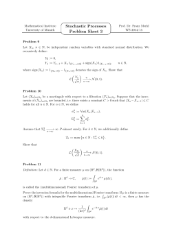
Fig. 1: Sample images for datasets used in this work.
Top:
UIUC [19], Middle: Virus [21], Bottom: TinyGraz03 [22].
To generate RCovDs, a feature vector is assigned to each
pixel at position (x, y) in an image I by
2 h
∂I ∂I ∂ I F(x,y) = IR (x, y), IG (x, y), IB (x, y), , , 2 ,
∂x
∂y
∂x
2 i
∂ I ∂y 2 , |G(0,0) (x, y)|, · · · , |G(u,v) (x, y)| , (9)
where Ic (x, y), c ∈ {R, G, B}, denotes color information, the
next four entries are the magnitude of intensity gradients and
the magnitude of Laplacians along x and y directions, and
G(u,v) (x, y) is the response of a 2D Gabor wavelet [20] centered at (x, y) with orientation u and scale v. We extracted
Gabor wavelets at four orientations and three scales. Therefore, each pixel is described by a 19 dimensional feature vector (i.e., 3 color, 4 gradients, and 12 Gabor features).
Table 1 shows the recognition accuracies for the studied
methods. The correct classification rates obtained by NN
clearly show that the proposed RCovDs are more discriminative than their low-dimensional counterparts. We also note
that NNF and NNN achieve comparable performances to
the more involved CDL in low-dimensional manifold.
The state-of-the-art performance on this dataset is 43.5%
reported by [19]. CDL on the proposed RCovDs (both random Fourier features and Nystr¨om) outperforms the state-ofthe-art performance by at least 2.8% percentage points.
5.2. Virus Classification
We performed an experiment to classify cell images using
the Virus dataset [21]. The dataset contains 1500 images of
15 different classes (100 samples per class). The images are
formed from Transmission Electron Microscopy technique
and re-sampled to 41 × 41 pixel grayscale image (see Fig. 1
for examples). Here, RCovDs are obtained using the features
described in Eq. (9) with one modification. For this task, we
used Gabor wavelets at four orientations and five scales.
Our empirical results are reported in Table 1. The average
correct recognition rate with both CDLF and CDLN is
superior to the state-of-the-art performance of 81.2% reported
in [1] using infinite-dimensional RCovDs. We conjecture that
computing the RCovDs with both random Fourier features
Method
UIUC
Virus
TinyGraz03
NN
NNF
NNN
CDL
CDLF
CDLN
26.5% ± 3.7
35.9% ± 3.0
35.6% ± 2.7
36.3% ± 2.0
47.4% ± 3.1
46.3% ± 2.6
58.8% ± 5.4
67.1% ± 4.2
69.5% ± 4.8
75.5% ± 2.5
82.5% ± 2.9
81.4% ± 3.1
34%
42%
44%
41%
55%
57%
and the Nystr¨om method reveals the nonlinear patterns in data
(as also evidenced in [11]). This is emphasized by the RieD
mannian structure of S++
(as CDL requires its tangent space)
which is not available for the infinite-dimensional RCovDs.
5.3. Scene Classification
For the last experiment, we considered the task of scene classification using TinyGraz03 dataset [22]. The dataset contains 1148 indoor and outdoor images (see Fig. 1 for examples) with a spatial resolution of 32 × 32 pixels.The images
are presented in 20 classes with at least 40 samples per class.
This dataset is quite diverse, with scene categories being captured from various viewpoints and under various lighting conditions. We used the recommended train/test split provided by
the authors. The correct recognition rate achieved by humans
on this dataset is 30% [22].
The RCovDs for this task were obtained using the first 7
features in Eq. (9) (i.e., 3 color and 4 image gradients). Table 1 indicates that computing RCovDs using random Fourier
features and the Nystr¨om method offers notable enhancement
in term of discriminatory power over the original RCovDs.
We also note that NNF and NNN outperform the more
involved CDL.
The state-of-the-art recognition accuracy on this dataset
is reported to be 46% [22]. Interestingly, CDLF and
CDLN significantly outperform the state-of-the-art method
(more than 9 percentage points) and human performance
(more than 25 percentage points).
6. CONCLUSIONS AND FUTURE WORK
We have made use of random Fourier feature and the Nystr¨om
method to compute two approximations to infinite-dimensional
RCovDs. Our experimental evaluation has demonstrated
that the proposed RCovDs significantly outperform the lowdimensional ones on image classification task. More importantly, our RCovDs provide a framework in which the
well-known Riemannian geometry of the SPD matrices can
be taken into account. In the future, we intend to explore
how the proposed approach can be extended to other types of
Riemannian manifolds, such as Grassmannian manifolds.
✁✂✄
7. REFERENCES
[1] Mehrtash T. Harandi, Mathieu Salzmann, and Fatih
Porikli, “Bregman divergences for infinite dimensional covariance matrices,” in Proc. IEEE Conference
on Computer Vision and Pattern Recognition (CVPR),
2014, pp. 1003–1010.
[2] Minh Ha Quang, Marco San Biagio, and Vittorio
Murino, “Log-Hilbert-Schmidt metric between positive
definite operators on Hilbert spaces,” in Proc. Advances
in Neural Information Processing Systems (NIPS), 2014,
pp. 388–396.
[3] Oncel Tuzel, Fatih Porikli, and Peter Meer, “Pedestrian
detection via classification on Riemannian manifolds,”
IEEE Transactions on Pattern Analysis and Machine
Intelligence (TPAMI), vol. 30, no. 10, pp. 1713–1727,
2008.
[4] Mehrtash T Harandi, Richard Hartley, Brian C Lovell,
and Conrad Sanderson, “Sparse coding on symmetric
positive definite manifolds using Bregman divergences,”
IEEE Transactions on Neural Networks and Learning
Systems, 2015.
[5] Masoud Faraki, Mehrtash T. Harandi, Arnold Wiliem,
and Brian C Lovell, “Fisher tensors for classifying human epithelial cells,” Pattern Recognition (PR), vol. 47,
no. 7, pp. 2348–2359, 2014.
[6] Xavier Pennec, Pierre Fillard, and Nicholas Ayache,
“A Riemannian framework for tensor computing,” Int.
Journal of Computer Vision (IJCV), vol. 66, no. 1, pp.
41–66, 2006.
[7] Sadeep Jayasumana, Richard Hartley, Mathieu Salzmann, Hongdong Li, and Mehrtash T. Harandi, “Kernel methods on the Riemannian manifold of symmetric
positive definite matrices,” in Proc. IEEE Conference
on Computer Vision and Pattern Recognition (CVPR),
2013, pp. 73–80.
[8] Masoud Faraki, Mehrtash T. Harandi, and Fatih Porikli,
“Material classification on symmetric positive definite
manifolds,” in Proc. IEEE Winter Conference on Applications of Computer Vision (WACV), 2015, pp. 749–756.
[9] Ali Rahimi and Benjamin Recht, “Random features for
large-scale kernel machines,” in Proc. Advances in Neural Information Processing Systems (NIPS), 2007, pp.
1177–1184.
[10] Christopher TH Baker, The numerical treatment of integral equations, Clarendon press, 1977.
[11] David Lopez-Paz, Suvrit Sra, Alex Smola, Zoubin
Ghahramani, and Bernhard Sch¨olkopf,
“Randomized nonlinear component analysis,” arXiv preprint
arXiv:1402.0119, 2014.
[12] Ali Rahimi and Benjamin Recht, “Weighted sums of
random kitchen sinks: Replacing minimization with
randomization in learning,” in Proc. Advances in Neural Information Processing Systems (NIPS), 2009, pp.
1313–1320.
[13] Quoc Le, Tam´as Sarl´os, and Alex Smola, “Fastfoodapproximating kernel expansions in loglinear time,” in
Proc. Int. Conference on Machine Learning (ICML),
2013.
[14] Rajendra Bhatia, Positive Definite Matrices, Princeton
University Press, 2007.
[15] Andrea Vedaldi and Andrew Zisserman, “Efficient additive kernels via explicit feature maps,” IEEE Transactions on Pattern Analysis and Machine Intelligence
(TPAMI), vol. 34, no. 3, pp. 480–492, 2012.
[16] Walter Rudin, Fourier analysis on groups, John Wiley
& Sons, 2011.
[17] Ruiping Wang, Huimin Guo, Larry S. Davis, and Qionghai Dai, “Covariance discriminative learning: A natural
and efficient approach to image set classification,” in
Proc. IEEE Conference on Computer Vision and Pattern
Recognition (CVPR), 2012, pp. 2496–2503.
[18] Roman Rosipal and Leonard J Trejo, “Kernel partial
least squares regression in reproducing kernel Hilbert
space,” Journal of Machine Learning Research (JMLR),
vol. 2, pp. 97–123, 2002.
[19] Zicheng Liao, Jason Rock, Yang Wang, and David
Forsyth, “Non-parametric filtering for geometric detail
extraction and material representation,” in Proc. IEEE
Conference on Computer Vision and Pattern Recognition (CVPR), 2013, pp. 963–970.
[20] Tai Sing Lee, “Image representation using 2d Gabor
wavelets,” IEEE Transactions on Pattern Analysis and
Machine Intelligence (TPAMI), vol. 18, pp. 959–971,
1996.
[21] Gustaf Kylberg, Mats Uppstr¨om, and Ida-Maria Sintorn,
“Virus texture analysis using local binary patterns and
radial density profiles,” in Progress in Pattern Recognition, Image Analysis, Computer Vision, and Applications, pp. 573–580. Springer, 2011.
[22] Andreas Wendel and Axel Pinz, “Scene categorization
from tiny images,” in 31st Annual Workshop of the Austrian Association for Pattern Recognition, 2007, pp. 49–
56.
✁✂✄