
The Biotope Method (PDF 3 MB)
The Biotope Method
A method for calculating the impact of land use and water use
March 2015
Content
Preface
Summary
1 Background 5
2 Purpose and objectives 6
3 Method
7
4 Step 1 – Delimitation
4.1 Introduction
4.2 System boundaries
8
8
9
5 Step 2 – Biotope Identification
5.1 General application
5.2 Application of the method in Sweden
10
10
13
6 Step 3 – Categorisation of biotopes
6.1 General application
6.2 Application of the method in Sweden
17
17
19
7 Step 4 – Reporting of results25
7.1 Quality level
25
7.2 Functional unit
26
7.3 The concept of life span
26
7.4 Reporting of results
26
8 References29
8.1 Literature
8.2 Web sources
Appendix 1 Guide to terrestrial biotopes31
Appendix 2 Guide to inland water and marine biotopes32
Appendix 3 Application of the method in Namibia and Australia36
Appendix 4 Review of the Biotope Method 201538
Preface
Vattenfall continuously work to improve our
environmental performance. One crucial element in
our work is to have a detailed understanding about
the environmental impacts linked to the full value
chain for our products. Vattenfall has for more
than 20 years worked with life cycle assessments
(LCA) and we have electricity generation certified
according to Environmental Product Declaration
(EPD) in accordance with ISO 14025. This means
that we have information on use of resources,
emissions, waste, recycling and land use for
every kilowatt hour of electricity generated. This
information we use proactively to reduce our
impacts on environment and to be transparent
towards our customers.
Protecting nature and species is one of Vattenfall’s
prioritised environmental topics. LCA standards
today give us insufficient guidance in how to
quantify and include impacts on biodiversity. As
a result, Vattenfall decided to develop the Biotope
Method in 1998-2000. The Biotope Method is a
standardised way to compare the state of different
biotopes before and after a development.
Now we have finished the update of the Biotope
Method 2015 and the method has been significantly
improved and takes new methods for assessing
impacts on biodiversity into account, for example
Helle Herk-Hansen,
Director Environment Vattenfall Norden
Stockholm, 2015-02-06
the new Swedish standards for biodiversity surveys.
It also takes into account the increased access
to digital information and additionally it includes
more information on how to assess changes in the
marine environment than the previous version.
With this update, Vattenfall has an even more
robust tool for assessing environmental impacts
from activities leading to a change in biotope
composition. Vattenfall will use the method to guide
us to further lower our impact on the biodiversity.
The Biotope Method 2015 has been developed
to be applicable in other areas than EPD, as well
as beyond the energy sector. We see that the
Biotope Method can be used with benefits in pilot
studies and location studies, to assess the impact
of planned operations. We hope that many others
will find the method useful and we are always
interested in getting input and ideas to improve
the method even further.
We would like to thank Eva Grusell, Sweco, for
her hard work with the revision. Also a special
acknowledgement to the project group, and to the
external reviewer Sofia Miliander, Sweco, for their
efforts in improving the Biotope Method.
Summary
Summary
This report presents a review and update of the
Biotope Method 2005.
The Biotope Method is based on the assumption
that the losses and additions of biotopes resulting
from exploitation mirror the resulting changes in
biodiversity. These losses and additions can be
quantified by measuring the areas affected, which
enables comparisons between different types
of exploitations. The use of the method entails
assessing the changes in the distribution and
quality of biotopes between ’before’ and ’after’
within a pre-defined area, i.e. the system boundary.
The Biotope Method is intended for use in
connection with most types of land and water
use. It is important to emphasise that the Biotope
Method only reports the quantitative biotope
changes (biotope losses and new additions) within
the system boundary. Exploitation may also entail
changes at the landscape level, i.e. outside the
system boundary. These may include changes such
as fragmentation, barrier effects and deterioration
of habitats. When the Biotope Method is used,
changes which take place beyond the system
boundary are described only qualitatively.
4
The Biotope Method
The Biotope Method 2015 has been developed
to be used also in areas of application other than
EPD, as well as beyond the energy sector. The
Biotope Method is also a tool which can be used
in feasibility-studies and localisation studies, to
assess the impact of planned operations.
Use of the Biotope Method obtains knowledge
of the impact of planned or ongoing operations
on biodiversity through the use of relatively
limited measures and resources. Input data for
the assessment is derived from available digital
databases, aerial images and project-specific
information. An inventory of biotopes is also
carried out in the field. If the Biotope Method is
used in a feasibility-study, the result can provide
suggestions for modifications; if the method is used
in a localisation study, it can generate suggestions
for prioritisation. If the Biotope Method is applied
to ongoing operations, the result can be used to
identify suggestions for biotope improvements and
compensation measures.
1 Background
1 Background
Work with Life cycle assessment (LCA) has for many
years been concerned with quantifying resource use
and emissions. Effects of land and water exploitation
on flora and fauna, on the other hand, have generally
been described only in general terms, and are very
rarely quantified.
In nature conservation biology, too, effects on
biodiversity at biotope and species level have
often been described only qualitatively. There are
quantitative measures concerning area data for land
and water which is protected by example national
parks, Natura 2000 areas and nature reserves. There
are also quantitative summaries of red-listed species
at national level.
5
The Biotope Method
As part of the work of preparing documentation
for environmental product declaration (EPD), the
Biotope Method was developed in Vattenfall in
order to quantify the effects on biodiversity (Blümer
& Kyläkorpi 1998, 2001). This was a voluntary
measure which resulted from the realisation that
the alternative, a merely qualitative description,
would be unsatisfactory. The method was initially
developed primarily for Swedish hydro power, to
deal with retrospective analyses. Between 1998 and
2005 the method was tested and further developed
through applications in many other aspects of
energy generation. Almost 10 years have passed
since the Biotope Method 2005 was developed. With
experience of the use of the Biotope Method 2005,
modifications and new knowledge, it is now time for
a review and update.
2 Purpose and objectives
2 Purpose and objectives
The aim of this report is to describe a method for
quantifying effects on biodiversity, which has been
developed and tested in Vattenfall. The ambition
is that the method will give a unified structure
that allows descriptions, quantifications and the
possibility of comparing different types of land use
and the resulting effects on biodiversity. It is used to
give standardised information concerning changes
caused by different types of land use – primarily
through biotope alteration, which are described
quantitatively but also qualitatively. The advantage
of this is that work on biotope improvements (nature
conservation measures) can also be quantified.
The Biotope Method was initially developed as a tool
to illustrate the environmental effect of electricity
and heat generation.
6
The Biotope Method
The purpose of the Biotope Method 2015 is:
•that it should be usable for studies of
changes in land and water use, both within
and beyond the energy sector.
•that it should be usable as a tool in feasibility
studies and location studies, in order to
assess the impact of planned operations.
The method should be usable even in cases
where time is limited, and with available data from
databases, aerial photography, etc., together with a
complementary site visit, when the delineated areas
are described in summary and verified. The method
is not intended to be an environmental impact
assessment, to result in detailed and complete
inventories of species or to give a full picture of
the effects on flora and fauna. It is important to
bear this in mind, since the method may entail
simplifications of things which are difficult to
describe quantitatively. A balance has to be struck
between completeness and simplification.
3 Method
3 Method
The Biotope Method is based on the assumption
that the loss and addition of biotopes resulting
from exploitation mirror the resulting changes in
biodiversity. These losses and additions can be
quantified by measuring the areas affected, which
enables comparisons between different types of
exploitations. The application of the method entails
the assessment of changes in the distribution and
quality of biotopes between situations ’before’ and
’after’ exploitation within a delimited area (the system
boundary of the investigation).
The Biotope Method is intended for use in connection with most types of land and water use. It is
important to emphasise that the Biotope Method only
reports the quantitative biotope changes (biotope
losses and any additions) within the system boundary.
Exploitation may also cause changes at the landscape
level, i.e. outside the system boundary. These may
include changes such as fragmentation, barrier effects and degradation of habitats. When the
Biotope Method is used, changes which take place
beyond the system boundary are described only
qualitatively. The Biotope Method is divided into four
steps (see Figure 1).
Figure 1. The four steps of the Biotope Method
Step 1
Delimitation
Information about the facility.
Determination of system boundaries.
Step 2
Biotope identification
Information about biotopes and their values
through existing inventory materials, aerial
photo interpretation and field visits.
Step 3
Biotope categorisation
In this step an assessment of the quality
of the biotopes is made.
Before
Critical biotope
Rare biotope
After
General biotope
Technotope
Step 4
Tabell 2. Indelningen av
biotoper utgår från Corine
Landuse level 2
Corine Level 1
Reporting of results
The operations will receive one of three quality
levels. The result is presented with descriptions,
maps, tables and are expressed per useful unit,
for example ha/kWh.
Corine Level 2
11 Urban fabric
12 Industrial, Commercial
and transport
13 Mine, dump and construction
sites
2 Agricultural areas
2
utgår från Corine Landuse level
Tabell 2. Indelningen av biotoper
Corine Level 1
21 Arable land
Corine Level 2
11 Urban fabric
transport
3 Forest and semi-natural
12 Industrial, Commercial and
areas
sites
13 Mine, dump and construction
21 Arable land
2 Agricultural areas
4 Wetlands
22 Permanent crops
23 Pastures
areas
24 Heterogeneous agricultural
3 Forest and semi-natural areas
5 Water bodies
31 Forests
31 Forests
32 Shrub and/or herbaceous
vegetation associations
33 Open spaces with little
or no vegetation
41 Inland wetlands
42 Coastal wetlands
51 Inland waters
vegetation associations
32 Shrub and/or herbaceous
no vegetation
33 Open spaces with little or
4 Wetlands
22 Permanent crops
23 Pastures
24 Heterogeneous agricultural
areas
52 Marine waters
41 Inland wetlands
42 Coastal wetlands
5 Water bodies
51 Inland waters
52 Marine waters
Depending on access to information about the
exploitation and the knowledge base concerning
the land and water areas affected, the results are
assigned to one of three possible quality levels.
The approach when using the Biotope Method is
always to achieve as high a quality level as possible.
If the operations under investigation are located on
geographically separate sites, a combined quality
level can be calculated from the total area used in
relation to the quality level of the individual plants.
7
The Biotope Method
When biotopes are categorised, an assessment is
made of their quality as habitats, e.g. naturalness,
the existence of certain structures, as well as the
occurrence of red-listed species or the diversity of
species. National assessment criteria are used in the
categorisation. An alternative approach can be used
in the event of limited access to species inventories
or other relevant information. The area in the ’before’
and ’after’ situations is in this case allocated in
accordance with a categorisation key that is further
described in chapter 6. The area of the technotope
must however always be known in the ’before’ and
’after’ situations.
4 Step 1 – Delimitation
4 Step 1 – Delimitation
4.1 Introduction
The first step of the Biotope Method is to establish
the system boundaries of the project in question. ’System boundary’ is used here with the meaning it
has in the context of LCA, i.e. the technical, geographical and temporal systems which are analysed
in a life cycle assessment. The impact which takes
place outside the system boundary should also be
established.
In short, the purpose of the delimitation stage is
to define what is to be included in the assessment
and what is to be excluded, both temporally and
spatially. The impact inside the system boundary
includes losses and additions of biotopes, which
should be quantified. The impact generally takes
place over a larger area than the more technicallyoriented system boundary. Impact beyond the
system boundary includes impact from a landscape
point of view, such as fragmentation, barrier effects
and degradation of habitats, which should be
described qualitatively.
Figure 2. System boundary
around a hydro power plant in
the Lule River in Boden
In order for the Biotope Method to be applicable, it
must be possible to determine the system boundary.
There should be information concerning the area
covered by the project and at least some information
concerning the direct impact of the operations in
order to achieve the lowest quality level. The extent
and quality of information sources determine how
the Biotope Method can be applied.
8
The Biotope Method
An important methodological limitation is that
the method does not include a step for analysing
potential compensation measures. On the other
hand, the method makes it possible to take account
of nature conservation measures in the reporting of
results.
4 Step 1 – Delimitation
4.2 System boundaries
Temporal delimitations
The ’before’ state is defined as the situation immediately before, or as close as possible to, the actual
requisitioning/exploitation. The ’after’ state is defined
as a point in time after exploitation, which usually
corresponds to the year in which the assessment is
carried out.
The time of biotope identification and biotope categorisation in both the ’before’ situation and the ’after’
state is always given. In the preparation of an EPD,
which is revised every three years, the ’after’ situation
is determined by the year in which the EPD is revised
and by basing the calculations on an updated value of
the functional unit. Biotope identification and biotope
categorisation for the ’after’ state do not need to be
carried out in the same year as the EPD is prepared,
but should not be carried out too long after the ’after’
situation, as the biotopes might have changed by
then. If the time of biotope identification and biotope
categorisation is different from the ’after’ situation
(e.g. EPD revision), the time of biotope identification
and biotope categorisation should be documented.
Since the method aims at analysing net effects, there
is no requirement to define a ’natural state’. The Biotope Method includes only the impact of the project
under investigation on the natural environment, with
subsequent changes in flora and fauna; it does not include anything done in the area earlier. In the Biotope
Method, only the effect of the individual project (i.e.
the net effect) is to be taken into consideration.
Spatial delimitation
It is important to define the spatial delimitation of
what is to be included in the study. The quantitative
assessment in the Biotope Method focuses on land
and water use which is directly connected with the
project under investigation and:
•has a clear geographical delimitation.
•is primarily not shared with other projects/interests.
The quantitative step therefore includes only the
direct impact which has arisen in the immediate
vicinity of the exploitation project. A road, a storage
area or a leisure area, for example, which is judged to
have very little connection with the project, can be
defined as beyond the system boundary. In practice,
this means that decisions have to be made on a case
to case basis regarding what should be included in
the assessment and what should be excluded. Proportions may also be calculated in cases where land
and water use is shared by a number of projects.
Delimitations should always be justified and reported.
9
The Biotope Method
There are certain differences of approach between
different types of land use. Below a number of examples concerning different types of energy sources are described.
The direct impact, i.e. within the system boundary,
from land and water use of an onshore wind power
project includes the requisition of land for works, roads and other related infrastructure. Wind energy
typically entails some form of impact beyond the system boundary, such as the fragmentation of habitats, the creation of barrier effects or collision risk for
birds.
The direct impact from land and water use of an
offshore wind power project includes the requisition
of areas for foundations, gravel beds etc., cables,
substations and weather masts. The impacts beyond
the system boundary take place both in and above the water. Examples of such impacts include reduced
feeding areas for certain marine species, barrier effects and collision risk for birds.
The direct impact from land and water use of a
hydro power plant can be complex. Along e.g.
Sweden’s major rivers, there are many hydro power
plants. Regulation of one reservoir may be used by
several different plants. The impact of a power plant
upstream in the water system can lead to impacts
downstream in the water system as well as in adjoining marine waters. Such impacts may include biotope loss or degradation of biotope quality, affecting
fish breeding and reproduction. In the application
of the Biotope Method on hydro power, the primary
focus has been on the study of reservoirs, dams,
spillways, dry water channels, switchgear, buildings
and roads associated with operations, run-off channels, extraction sites, storage areas, fillings, embankments and affected beaches downstream. In the case of reservoirs, adjacent reservoirs are
included within the system boundary.
The direct impact from land and water use of a nuclear power facility does not only concern the
nuclear power plant where electricity is generated.
The entire fuel chain is regarded as being within the
system barrier - i.e. the uranium mines, conversion and
enrichment plants, fuel production plants, the nuclear
power plants and waste facilities. In the case of a
nuclear power plant, the cooling water plume is also
included within the system boundary.
In a corresponding manner as for nuclear power, the
system boundary for coal power includes the entire
fuel chain - i.e. the mines, transhipment harbours,
power plants and waste management facilities.
5 Step 2 – Biotope identification
5 Step 2 – Biotope identification
5.1 General application
The second step in the application of the Biotope
Method is the identification of the biotopes which
have been affected. The biotopes should be identified
both in the ’before’ and the ’after’ situations, so that
an assessment can be made of the changes related
to the requisition of land and water areas. The focus
is on collecting information on the area within the
system boundary, where quantification takes place in
accordance with the Biotope Method. Depending on
the nature of the operations, i.e. whether there is also
an impact beyond the system boundary, data should
be collected in a larger area in order for the impact
to be described qualitatively. The amount of detail
in the description of qualitative impact beyond the
system boundary depends on the purpose of applying
the Biotope Method. The qualitative impact can be
described in detail or summarised as a list of points.
The purpose of the identification is to produce as
much knowledge as possible about the land and
water areas within the area being studied. The step
of biotope identification also includes identifying
areas which lack preconditions for biological
production. GIS data, existing inventories, aerial
photographs, site visits etc. provide a basis for the
identification of biotopes in the ’before’ and ’after’
situations. If a site visit in the ’after’ state enables
an impression to be formed of the ’before’ situation,
observations made during the site visit can be used
as a basis for a description of the ’before’ situation.
The information collected for biotope identification
determines the quality of the categorisation in
step 3. There are alternative types of procedure,
depending on accessibility and quality of information
(see Table 9).
Figure 3. Seitevare hydro power plant in the Lule river, biotopes in the ’before’ situation
10 The Biotope Method
5 Step 2 – Biotope identification
Corine landuse (Bossard 2000) is used as the
basis for the classification of biotopes. A national
interpretation is made of level 2 (see Table 2).
The classification is based on habitat types,
vegetation types, hydro morphology/soil types or
geomorphology/rock types, depending on national
Collection of available information concerning
known conditions:
•Information from available digital databases.
•Material from previously performed
inventories.
•Information concerning the plant’s land
and water requirements, situation maps,
environmental impact assessment, etc.
•Collect existing information and document
the sources and the date.
11 The Biotope Method
conditions (see Table 4 - Table 7). Biotopes are
described on the basis of naturalness, structures
and continuity etc. The description is complemented
by the known incidence of species such as indicator
species and ‘conservation species’, as well as
diversity of species.
Identification of biotopes:
•Interpretation of aerial photographs (if
possible)
•Field visit (if possible).
•Descriptions on the basis of Corine landuse
(see Table 2). The categorisation is based
on national conditions and the biotopes are
described on the basis of national practice.
•If there is also an impact beyond the system
boundary, data is collected for a larger area.
•Calculation of areas.
5 Step 2 – Biotope identification
Table 1. Information sources
Information sources
Commentary/description
Maps
Aerial photographs/orthophotos/IR
Satellite images
Topographic map
Soil type map
Plant-specific information
Situation maps
Environmental impact assessment
Knowledge base concerning known values
Digital info for GIS
Inventory reports
Site visit
Surveying of conditions on site and verification of known
information
Table 2. Categorisation of biotopes is based on Corine landuse level 2
Corine Level 1
Corine Level 2
1 Artificial surfaces
11 Urban fabric
12 Industrial, commercial and transport
13 Mine, dump and construction sites
14 Artificial, non-agricultural vegetated areas
2 Agricultural areas
21 Arable land
22 Permanent crops
23 Pastures
24 Heterogeneous agricultural areas
3 Forest and semi-natural areas
31 Forests
32 Shrub and/or herbaceous vegetation associations
33 Open spaces with little or no vegetation
4 Wetlands
41 Inland wetlands
42 Coastal wetlands
5 Water bodies
51 Inland waters
52 Marine waters
12 The Biotope Method
5 Step 2 – Biotope identification
5.2 Application of the method in Sweden
Information concerning known conditions can be
taken from digital databases supplied by authorities.
This includes information on protected areas,
woodlands, agricultural land, meadows and pastures,
wetlands, red-listed species and other rare species,
catchment areas, water protection areas, soil types
and data from sampling and environmental monitoring.
Digital map material can be obtained for ground
maps, current and historic aerial photographs, satellite
images and soil type maps, etc. (see Table 3).
The categorisation of biotope/habitat types to
be found in nationwide inventories of terrestrial
environments is also used in the Biotope Method.
Categorisation of biotopes in lakes and watercourses
is based on the hydro morphological conditions.
Categorisation of marine biotopes is based on the
type of seabed. If a Natura 2000 habitat appears,
this is indicated and named as such.
Table 3. Information sources
Maps
Collected/delivered from:
Aerial photographs/orthophotos/IR
Land Survey
Satellite images
Land Survey
Map of soil types
Geological Survey of Sweden
Ground maps etc.
Land Survey etc.
Plant-specific information
Situation maps
Operator
Environmental impact assessment
Operator, authorities
Knowledge base concerning known values
Digital info for GIS
National, regional and local databases, e.g. Swedish Environmental
Protection Agency (protected areas), Environmental data portal
(Miljödataportalen), Geological Survey of Sweden (soil ets), Swedish
Meteorological and Hydrological Institute (waterweb), Sweden´s
five water agencies (VISS portalen), The Swedish Species
Information Centre (Artportalen and Trädportalen) , Swedish
Board of Agriculture (database about agriculture land and, TUVA
- database of meadow and pasture inventories), Swedish Forest
Agency (database about values in the forest), Swedish University
of Agricultural Sciences ((Forest Map) and Swedish Environmental
Protection Agency (System Aqua).
Inventory reports
A knowledge base can be derived from various inventories. These
have national, regional or local distribution. The national and regional
documents produced by authorities have been partly digitalised - see
above. There are also various reports produced by experts.
The artificial areas
The artificial areas are described on the basis of
information from the operator and observations
made during the site visit. If vegetation appears in
association with roads, power lines, airports etc.,
the so-called green infrastructure, the biotope is
described on the basis of their habitats they provide
and the species they support.
Table 4 .The artificial areas
Corine level 2
Level 3 - National interpretation: examples of biotopes or
technotopes
11 Urban fabric
Hard-made surfaces, buildings
12 Industrial, commercial and transport
Roads, turning areas, railways, switchgear
13 Mine, dump and construction sites
Slag heaps, storage areas, open-pit mines, quarries
14 Artificial, non-agricultural vegetated areas
Lawns, parks
13 The Biotope Method
5 Step 2 – Biotope identification
Terrestrial biotopes
There are a number of nationwide biotope inventories of terrestrial environments, such as the key
biotope inventory (forests with value), wetland
inventory and meadow and pasture inventory. There
is a relatively good knowledge of the most valuable
biotopes, which are included in these national inventories. Protected areas are often well documented.
For example, there are management plans available
for nature reserves and habitats within Natura 2000
areas. The naming used in the national inventories
and within protected areas can be used in the description of values. In appendix 1 there is a compilation of national and regional knowledge bases, which
should always be taken into account. There is
additional support for the naming of biotopes in the
technical report (SIS-TR 199001:2014) associated
with the Swedish Standard Institute (SIS) standard
for Biodiversity survey - Implementation, assessment
and reporting (SIS-SS 199000:2014).
The terrestrial biotopes are identified initially on the
basis of an aerial orthophoto interpretation. Complementary information is taken from the digital databases and any available inventory reports. During the
site visit, an inventory of biotopes is made and the
biotopes are classified on the basis of the methodology in the national inventories referred to above.
Table 5. Terrestrial biotopes
Corine level 2
Level 3 - National interpretation: examples of biotopes
21 Arable land
Ploughable arable land
22 Permanent crops
Fruit and berry cultivation etc
23 Pastures
Different types of maintained meadow and pasture
24 Heterogeneous agricultural areas
Mixed cultivation, agroforestry etc
31 Forests
Different types of woodland such as coniferous forest, deciduous
woodland, broad-leaved deciduous woodland, alder fen and
marsh woodland, older solitary trees and groves
32 Shrub and/or herbaceous vegetation associations
Different types of bush areas such as willows, hazel groves and
forests edges
33 Open spaces with little or no vegetation
Sandy environments, e.g. sand dunes and sandy moorlands
41 Inland wetlands
Different types of wetland and rich fen
42 Coastal wetlands
Different types of beach and water environments
Photo Eva Grusell
14 The Biotope Method
5 Step 2 – Biotope identification
Inland water biotopes
Knowledge concerning biodiversity in lakes and
watercourses is relatively good, but there is a lack of nationwide inventories. Also in the inland water environments, there are protected areas with associated documentation of their value, e.g. Natura 2000
habitats and nationally designated areas of nature
protection. In recent years, a number of criteria for
the assessment of natural value have been presented, including System Aqua and inland water key
biotopes. During 2013, the Swedish Agency for Marine and Water Management produced regulations for the classification and environmental quality
norms of inland water. These also include assessment
criteria for hydromorphological quality factors in
lakes and watercourses.
There is information concerning lakes and watercourses produced in connection with environmental
monitoring. Information relating to water chemistry,
phytoplankton, lake and river bed fauna, obstacles to migration and water vegetation are collected in
the Environmental Data Portal and VISS portal databases. Other inventories have also been made of sea birds, otters and mussels, for example. Overall,
lakes and watercourses in southern and central
Sweden are better mapped than those in northern
Sweden.
The inland biotopes are initially identified (see Table 6) on the basis of an interpretation of aerial
photography of the hydromorphological conditions,
with complementary information concerning soil
types. The biotopes are then classified according
to hydromorphological types - see Appendix 2.
The Swedish Agency for Marine and Water
Management’s assessment criteria for hydromorphological quality factors in lakes and watercourses
(HVMFS 2013:19) are used for this classification.
Complementary information concerning the area’s
status is taken from the digital databases, such as
the VISS portal, and any inventory reports which may
be available. During the site visit, a study is made of
the degree of naturalness/impact in the inland water
biotope and surrounding area.
Table 6 Inland water biotopes
Corine level 2
Level 3 - National interpretation: examples of biotopes
51 Inland waters
Steep watercourses in solid rock, Steep watercourses with
stones and turbulent flow, Broad watercourses with regularly
alternating reaches and pools, Watercourses with a number of
parallel channels, Meandering watercourses, Over-deepened
watercourses in fine-grained sediment, Watercourses in peat
Lakes in tectonic basins, Lakes in glacial erosion basins, Glacial
damming basins, Natural non-glacial lakes, Artificial lakes,
Artificial waters
Photo Eva Grusell
15 The Biotope Method
5 Step 2 – Biotope identification
Marine biotopes
Today’s knowledge base for the marine environments
is not all-encompassing. Threatened biotopes in the
Baltic Sea are listed in HELCOM (HELCOM 1998,
2006) and a biotope classification of threatened
and representative coastal biotopes was made in
’Kustbiotoper i Norden’ (’Coastal biotopes in the
Nordic region’) (Nordic Council of Ministers 2001).
The Swedish Environmental Protection Agency
has produced a guide to the protection of marine
environments. Otherwise there are only a number of
inventories, samples and models of the distribution
of species and biotopes. Some data on marine
environments is available via the VISS portal. The
Swedish Agency for Marine and Water Management
has begun work to produce a national method of
marine natural value assessment.
The marine biotopes (see Table 7) are described
on the basis of information in the VISS portal and
any available reports concerning on-site conditions.
Appendix 3 contains a description of the marine
habitats.
Table 7. Marine biotopes
Corine level 2
Level 3 – National interpretation: examples of biotopes
52 Marine waters
Shallow marine soft seabed,
Shallow marine hard seabed,
Deep marine soft seabed,
Deep marine hard seabed,
Biogenic reefs and bubble reefs,
Anthropogenic marine seabed.
16 The Biotope Method
6 Step 3 – Categorisation of biotopes
6 Step 3 – Categorisation of biotopes
6.1 General application
During the categorisation step, an assessment of
the quality of the biotopes is made. Based on their
ecological characteristics, the biotopes are divided
into four different categories: critical biotopes, rare
biotopes, general biotopes and technotopes. When
applying the Biotope Method, national assessment
criteria should be used as a basis. A biotope is
assessed on the basis of its quality as a habitat,
as well as the existence of certain structures and
the incidence of red-listed species, signal species,
‘conservation species’, as well as diversity of species.
The Swedish SIS standard for Biodiversity survey
- Implementation, assessment and reporting
(SIS-SS 199000:2014) was used as the basis for
constructing the hierarchy and formulating the
general criteria. An important difference is that,
while the Biotope Method uses species as a support
for the assessment of biotopes, the SIS standard for
Biodiversity survey - Implementation, assessment
and reporting assesses species and biotopes
separately.
Table 8 The biotopes are divided into four categories.
Category
Definition
Critical biotope
Highest or high natural value: an area categorised as a critical biotope is judged to have particular
importance for the preservation of biodiversity on a global, national and regional level. The area
has a much greater diversity of species than the surrounding landscape or other areas of the same
biotope in the region or country. All Natura 2000 habitats are categorised as critical biotopes.
There are red-listed species in the area.
Rare biotope
Substantial natural value: an area categorised as rare biotope need not have particular importance
for the preservation of biodiversity at regional, national or global level. The area is judged to have
particular importance for the maintenance or growth of the total extent of such areas, and for the
maintenance or improvement of their ecological quality. A rare biotope may, in the long term or with
restoration measures, reach critical biotope status. A rare biotope has a greater diversity of species
than the landscape in general, and is of importance for landscape variation. Isolated red-listed
species or key elements occur.
General biotope
Minor natural value: an area categorised as general biotope consists of commonly occurring habitats
- the so-called everyday landscape. The general biotope also includes trivial areas where biological
production occurs, e.g. planted green spaces in urban environments.
Technotope
Areas lacking preconditions for biological production.
The best categorisation results are obtained when
there has been good access to information for
biotope identification (step 2) for both the ’before’
and ’after’ situations. In this case all areas should be
delineated, and every biotope described. In Table 11
there is a review of the quality levels of the Biotope
method and requirements of the different levels for
documentation.
If access to inventory material is limited, there is an
alternative type of procedure which can be used. In
the ’before’ and ’after’ states, the area is divided in
accordance with categorisation keys (see Table 9).
In these cases the areas are categorised directly,
without prior identification. The technotope must be
known in the ’before’ or ’after’ states. The purpose of
17 The Biotope Method
the keys is to enable a standardised categorisation
of the original and/or resulting areas, with a reasonable margin of error. The categorisation keys are
produced with a high degree of conservatism. Their
main purpose is that they should only be used in
case of extremely limited access to information. The
proportions between the categories in the categorisation keys are judged to be sufficiently well worked
out that the disturbances caused by the use of the
area are, by a wide margin, not underestimated. This
means that the categorisation keys should always
overestimate critical and rare biotopes in the ’before’
situation, and always underestimate them in the
’after’ situation. There should therefore be no risk
of these keys being used to quickly reach a result
which is more favourable for the operator.
6 Step 3 – Categorisation of biotopes
Table 9. Categorisation with the aid of categorisation keys, where there is a lack of information for biotope identification in the ’before’ or
’after’ situation
Categorisation key [F] for ’before’ situation
Categorisation key [E] for ’after’ situation
The area T* is measured, and the remaining area is assumed
to comprise 40 % critical biotope, 40 % rare biotope and 20 %
general biotope.
The area T is measured, and the remaining area is assumed to
consist of general biotope.
* If it is impossible to establish the area T, the value is assumed to be 100 % of the affected area in the ’after’ situation, and 0 % in the
’before’ situation.
Figure 4. Forsmark nuclear power plant, categories in the ’after’ state. GB = General Biotope, T = Technotope
18 The Biotope Method
6 Step 3 – Categorisation of biotopes
6.2 Application of the method in Sweden
The categorisation of biotopes is based on the SIS
standard for Biodiversity survey - Implementation,
assessment and reporting (SIS-SS 199000:2014),
but certain modifications have been made to adapt
it to EPD, feasibility studies and localisation studies.
Biotopes and species are not assessed separately
in the Biotope Method; species are, rather, used as
a support in assessing biotopes. In other respects,
the terrestrial biotopes follow the SIS standard and
the associated technical reports. Sweden does not
have generally accepted assessment criteria for
marine and inland water habitats, of the kind it has
for terrestrial habitats. In comparison with the SIS
standard for nature value inventory, a modification
has been made for the inland water and marine
environments in the Biotope Method. The reason
for this is to adapt the method to the ongoing work
on assessment criteria by the Swedish Agency for
Marine and Water Management.
There are national assessment criteria for a number
of terrestrial environments such as Natura 2000
habitats, wetlands, key biotopes for woodland,
meadow and pasture land. In the SIS standard, the
assessment criteria for the terrestrial environments
are harmonised.
There are no national assessment criteria for inland
water environments, but there are documents and
criteria in the Natura 2000 habitats, ’System aqua’
and ’Limniska nyckelbiotoper’ (’Inland water key
biotopes’) as well as information in the VISS portal.
Access to information for individual sites varies. The
ecological status in the VISS portal can be used
if there is no other information to use as a basis
for categorisation. The Swedish Agency for Marine
and Water Management is working to produce
assessment criteria for inland water environments:
for watercourses in autumn 2014 and for lakes in
spring 2015.
There are no national assessment criteria for
marine environments. Natura 2000 habitats, the
HELCOM list of threatened biotopes in the Baltic
Sea, ’Kustbiotoper i Norden’ (’Coastal biotopes
in the Nordic region’) – biotope classification of
threatened and representative coastal biotopes and information in the VISS portal can be used to
support assessment. Access to information for the
individual sites varies, and is considerably more
limited than for the inland water environments. The
ecological status in the VISS portal can be used if
there is no other information to use as a basis for
categorisation. During 2015, the Swedish Agency
for Marine and Water Management will initiate a
more comprehensive work on assessment criteria
for marine environments.
Table 10. The Biotope Method’s categories, and how they correspond to the SIS standard and VISS portal
Category
Equivalent in SIS standard
Corresponds to current water status*
Critical biotope
Nature value class 1 and 2
High ecological status
Rare biotope
Nature value class 3
Good ecological status
General biotope
Nature value class 4 and all green spaces
with biological production
Moderate ecological status
Technotope
Areas lacking preconditions for biological
production
* In the absence of information, ecological status can be used for categorisation 19 The Biotope Method
6 Step 3 – Categorisation of biotopes
Table 11. Classification of biotopes into four categories and their definitions
Critical biotope (SIS class 1 och 2)
General criteria
An area categorised as critical biotope is judged to have particular importance for the
preservation of biodiversity on a global, national and regional level. The area has a
much greater diversity of species than the surrounding landscape or other areas of
the same biotope in the region or country. All Natura 2000 habitats are categorised as
critical biotopes. Aquatic environments judged to have a high ecological status.
A number of protected species / isolated red-listed species occur.
Criteria in Sweden
The marine biotopes
Clarification
Shallow seabed
Species-rich and unaffected, or affected to some extent, by human intervention
Examples of soft seabeds:
•Shell gravel banks, lagoons, deltas and sea wrack meadows
Examples of hard seabeds:
•Blue mussel beds, caves, reefs, vertical surfaces and algae belts
Deep seabeds
Species-rich and unaffected, or affected to some extent, by human intervention
Examples of soft seabeds:
•Seabeds have not been bottom-trawled or damaged by lack of oxygen
•Sea pens and scallops are species which may indicate higher value
Examples of hard seabeds:
•Fiords or other protected sites, vertical surfaces, caves and areas which are important for fish,
benthic animals and corals
Biogenic reefs and bubble reefs
Seabeds can even be considerably affected by human intervention
Example:
•Coral reefs, blue mussel banks and oyster beds
Anthropogenic marine seabed
Seabeds should contribute towards variation in soft seabeds
Example:
•Establishment of man-made substrates with fouling of mussels, cnidarians and ascidians
•Blue mussel beds and algae belts with distinct zoning
The inland water biotopes
Clarification
Lakes
Example:
•Lakes with important reproduction areas and growth environments for fish, birds, etc
•Lowland lakes with substantial aquatic vegetation and rich birdlife
•Charophyceae lakes
•Nutrient-poor clear water lakes with zoned underwater vegetation
•Naturally dystrophic lakes and lakes with islands, bare rocks, beach cliffs, rocks, bird cliffs and
reefs
•Lakes with long turnover time, pelagic fish fauna and high plankton biodiversity
•Large, variegated, deep lakes with good nutrition status, water quality and incidence of deep
gravel lake beds which function as breeding grounds and growth areas for fish
•Naturally clear and nutrition-poor lakes with ice-age relics
Small bodies of water
Example:
•Naturally dystrophic small bodies of water, mire lakes
•Clay pits
•Small bodies of water with rich fen vegetation
•Breeding waters for frogs and lesser water salamanders
Continued table next page
20 The Biotope Method
6 Step 3 – Categorisation of biotopes
Continued table
Watercourses
Example:
•Block-rich unaffected reach
•Unaffected ravine reaches with surrounding ravine woodland
•Larger natural bifurcation areas
•Gently-flowing reaches across extensive open water land with substantial incidence of wellgrazed and/or open shores
•Long meanders
•Rapids, unaffected reach with waterfalls
•Sandy erosion slopes
•Outflow areas
•Estuary areas and deltas
The terrestrial biotopes
Clarification
Woodland
Example:
•Key biotopes
•Deciduous woodland inventory class 1 and 2
•High-grade deciduous woodland inventory class 1 and 2
Wetlands
Example:
•VMI class 1 and 2
•Rich fen inventory class 1, 2 and 3
Meadow and pasture land
Example:
•The Swedish Board of Agriculture’s meadow and pasture land - active sites (TUVA)
Trees
Example:
•Trees worthy of protection, as in programme of measures
21 The Biotope Method
6 Step 3 – Categorisation of biotopes
Rare biotope (SIS class 3)
General criteria
An area categorised as rare biotope need not have particular importance for the
preservation of biodiversity at regional, national or global level. The area is judged
to have particular importance for the maintenance or growth of the total extent of
such areas, and for the maintenance or improvement of their ecological quality. A
rare biotope may, in the long term or with restoration measures, reach critical biotope
status. A rare biotope has a greater diversity of species than the landscape in general,
and is of importance for landscape variation. For example, aquatic environments
judged to have a good ecological status are included. Isolated protected species / redlisted species occur, or occurrence of key elements.
Criteria in Sweden
The marine biotopes
Clarification
Shallow seabed
All hard and soft shallow seabeds, but not completely impoverished
Deep seabeds
Soft seabeds are affected to some extent by human intervention
Hard seabeds may even be affected by trawling
Biogenic reefs and bubble reefs
Seabeds may even by heavily affected by human intervention, but still with occurrence of reefforming species
Anthropogenic marine seabed
Anthropogenic seabed, as it can contribute to creating variation in soft seabeds without identified
red-listed species
The inland water biotopes
Clarification
Lakes and small bodies of
water
More or less natural lakes and small bodies of water which have been subject to minor or moderate
human intervention
Artificial and regulated lakes and small bodies of water, with a degree of naturalness and with
importance for the preservation of biodiversity
Watercourses
Example:
•Block-rich, partly affected reach
•Smaller bifurcation area, partly affected
•Meandering watercourse, shorter stretch
•Rapids, partly affected stretch with waterfalls
The terrestrial biotopes
Clarification
Woodland
Example:
•National Board of Forestry sites with natural value or equivalent value
Wetlands
Example:
•VMI (Wetland Inventory) class 3 with value concentrations or equivalent value
Meadow and pasture land
Example:
•The Swedish Board of Agriculture’s ’restorable meadow and pasture land’ or equivalent value
Trees
Trees with potential protection value
22 The Biotope Method
6 Step 3 – Categorisation of biotopes
General biotope (SIS class 4 + preconditions for biological production)
General criteria
An area categorised as general biotope consists of commonly occurring habitats, the
so-called everyday landscape. The general biotope also includes trivial areas where
biological production occurs, for example planted green spaces in urban environments.
Aquatic environments judged to have a moderate ecological status.
Criteria in Sweden
The marine biotopes
Clarification
All
Certain values and/or trivial marine habitats with biological production
The inland water biotopes
Clarification
All
Certain values and/or trivial inland water habitats with biological production
De terrestra naturtyperna
Clarification
All
Certain values and/or trivial green areas with biological production
Technotope
General criteria
Areas lacking preconditions for biological production.
Criteria in Sweden
Technotopes
Clarifications
E.g. buildings, roads, car parks, aquatic environments with no biological life
23 The Biotope Method
6 Step 3 – Categorisation of biotopes
General biotope
Critical biotope
Technotope
Critical biotope
Technotope
Rare biotope
Figure 5. Examples of biotopes divided into categories
Photo Eva Grusell
24 The Biotope Method
7 Step 4 – Reporting of results
7 Step 4 – Reporting of results
7.1 Quality level
The quality of the result depends on the extent to
which input data is available, and on the efforts and
resources the operator is prepared to invest in the
study. The results can be reported according to various quality levels. In short, it may be said that the
more information is available and the more time is
devoted to data collection and analysis, the higher
the quality level it is possible to achieve. In Table 12
details are given of the requirements concerning
inventory material for the different quality levels.
A project in a geographical situation
Quality level A is achieved when satisfactory inventory material is available for both ’before’ and ’after’
situations. This result in identified biotopes and categorised areas, classified into the Biotope Method’s
four categories: critical, rare and general biotopes,
and technotopes. Quality level B is achieved if inventory material is lacking either ’before’ or ’after’: B1 if
there is inventory material for the ’before’ state and
B2 if there is inventory material for the ’after’ state. If
inventory material is lacking for both the ’before’ and
’after’ states, quality level C is achieved.
Table 12. Quality levels and requirements for inventory material for the ’before’ and ’after’ states
Quality level
Before
After
A
•Inventories in the field or
•Satisfactory inventory material or
•Aerial photography interpretation, incl.
verification of red-listed species and values
•Site visit (though exceptions are possible) and
•Inventories in the field or
•Satisfactory inventory material or
•Aerial photography interpretation, incl. verification
of red-listed species and values
B1
•Inventories in the field or
•Satisfactory inventory material or
•Aerial photography interpretation, incl.
verification of red-listed species and values
•Categorisation key
B2
•Categorisation key
•Site visit (though exceptions are possible) and
•Inventories in the field or
•Satisfactory inventory material or
•Aerial photography interpretation, incl. verification
of red-listed species and values
C
•Categorisation key
•Categorisation key
Several projects with geographical spread
Whether quality level A, B or C is achieved depends on the combined quality of the inventory
material for the plants included. The precision of
the figures is also reflected in the combined quality level. In Table 13 details are given of how the
quality level is calculated.
Table 13. Calculation of quality levels if several plants with geographical spread are included in a study
Quality level Weighted
Explanation
A
≥75 % of the total area has been carried out as in A
B
≥75 % of the total area has been carried out as in A or B (A+B≥75 %)
C
Other cases
25 The Biotope Method
7 Step 4 – Reporting of results
7.2 Functional unit
The term ’functional unit’ is taken from the
methodology of life cycle assessment (LCA). It
means the unit of produced good which is used
as a measure of comparison or efficiency. If the
biotope impact measured by the Biotope Method is
to be used to compare the efficiency of two ways
of producing the same good, it has to be related to
such a functional unit.
Example of calculation:
In the case of electrical energy, for which the
Biotope Method was originally developed, this unit
is the kWh. Other units, such as MWh or GJ, can of
course also be used, but the important thing is to be
consistent in reporting all impact in relation to the
same unit.
Impacted Area (m2 or ha)
Life span (y) × Functional Unit (e.g. kWh)
= Area per Functional Unit (e.g. m2/kWh)
7.3 The concept of life span
The biodiversity will be affected for at least as long
as the operations continue on the specific site. The
degree of impact is determined by the situation in
the chosen ’after’ state. The longer the life span
used in calculating the result, the smaller will be
the impact per unit of usefulness, since the biotope
impact is assumed to be constant during the entire
life span. If the study of operations forms part of
an environmental product declaration (EPD) which
is revised every three years, for example, there is
a possibility of updating the biotope impact. The
quality of a biotope may, in time, improve as well as
deteriorate.
In the context of life cycle assessments, the life cycle
of a plant is considered, from the cradle to the grave,
and the length of the life cycle is determined by the
life span of the components included. A plant may
of course be modernised or even replaced entirely,
and thus acquire a longer life span than the technical
components included. It is likely, for example, that
wind power turbines will stand in a favourable location
for longer than 25 years, and that hydropower dams
can exist for much longer than 100 years. When
the Biotope Method is applied in connection with a
life cycle assessment (LCA) or in an environmental
product declaration (EPD), however, the same
temporal system boundary is used as in the LCA.
7.4 Reporting of results
Data generated in a life cycle assessment and
other methods of environmental analysis must be
presented in a standardised manner. It is important
that reporting of relevant information, input data,
assessments conducted and final results is done in
a transparent fashion.
Table 14. Reporting of results
Quality level
A
B1
B2
C
26 The Biotope Method
Descriptions with
rationale concerning
System boundary
Identification
Categorisation
Systemgräns
Maps
Identification
Maps
categorisation
Tables
Significant
figures
Before and After
Before and After
Before and After
3
Before
Before
Before and After
2
After
After
Before and After
2
Before and After
1
-
7 Step 4 – Reporting of results
Example of calculation for an operation with three
plants with 100 years’ technical life span
The areas in each biotope category related to
electricity generation in each plant are shown
in Table 15. Electricity generation in all plants is
assumed to be 40 TWh over 100 years.
Table 15. Example of calculation of change of surface area per unit of usefulness (m2/kWh) for three plants with different quality levels
(The values in the table have been rounded off, since they are here used for the purpose of illustration.)
Plant with quality
level
Category
Area ’before’ (ha)
Area ’after’ (ha)
Biotope change
(ha)
A
Critical biotope
400
0
-400
-10,0 x 10⁻⁶
Rare biotope
400
0
-400
-10,0 x 10⁻⁶
General biotope
200
500
300
7,5 x 10⁻⁶
Technotope
0
500
500
12,5 x 10⁻⁶
Critical biotope
1 000
200
-800
-20,0 x 10⁻⁶
Rare biotope
600
300
-300
-7,5 x 10⁻⁶
General biotope
300
500
200
5,0 x 10⁻⁶
Technotope
100
1 000
900
22,5 x 10⁻⁶
Critical biotope
40
10
-30
-0,75 x 10⁻⁶
Rare biotope
40
20
-20
-0,5 x 10⁻⁶
General biotope
20
20
0
0
Technotope
0
50
50
1,25 x 10⁻⁶
B
C
The application of the Biotope Method to the plants
achieves the combined quality level B, since more
than 75 % of the total area has been carried out in
accordance with either A or B - see Table 16. The
result is thus reported with two significant figures.
Table 16. Total area requisitioned, divided into quality levels
Quality level
Areal (ha)
%
A
1,000
32
B
2,000
65
C
100
3
3,100
100
Total
27 The Biotope Method
Change per kWh
of electricity (m2/
kWh electricity)
7 Step 4 – Reporting of results
Table 17 is a summary of biotope changes for the
three plants related to net electricity generated (120 TWh over 100 years’ normal generating).
The combined biotope changes for the plants in the
table below represent a considerable simplification.
But the table does give a rough estimate of the
direct biotope changes caused by the operations.
The results should be interpreted on the basis of the
whole report.
Table 17. Combined change of area per unit of usefulness
Category
Critical biotope
Rare biotope
General biotope
Technotope
Biotope change (ha)*
Change per kWh of electricity
(m2/kWh electricity)
-1,200
-10 x 10-6
-720
-6,2 x 10⁻⁶
500
4,2 x 10⁻⁶
1,400
12 x 10-6
* Rounding off to two significant figures sometimes entails, as in this example, that the sum of biotope changes is not zero.
28 The Biotope Method
8 Referenser
8 References
8.1 Literature
A
Artdatabanken 2010. Rödlistade arter i
Sverige.
Artdatabanken 2014. Arter och naturtyper
i habitatdirektivet – bevarandestatus i
Sverige 2013.
B
Bleckert, S., Degerman, E., Henrikson, L. &
Pettersson, R. 2010: Skogens vatten – Om
naturhänsyn i skogsbruket. Södra Skogsägarna, Mellanskog, Norrskog och Norra
Skogsägarna.
Bossard, M., Feranec, J. & Otahel, J. 2000.
CORINE land cover technical guide – Addendum 2000. Technical report No 40.
European Environment Agency.
Burke, A. 2005. Biotope mapping, reconstruction of the pre-mining situation and
assessment of biodiversity value. Phase
2 Report. Report to Rössing Uranium Ltd,
Swakopmund.
Burke, A., Kyläkorpi, L., Rydgren, B. &
Schneeweiss, R. (2007) Testing a Scandinavian Biodiversity Assessment Tool in an
African Desert Environment. Environmental
Management (2008) 42:698–706.
E
Energimyndigheten 2014. Vad avgör ett
vattenkraftverks betydelse för elsystemet Underlag till nationell strategi för åtgärder
inom vattenkraften. ER 2014:12.
G
Gardener, M. 2007. Assessing the impact
of land use at ERA on biodiversity using
Vattenfall’s Biotope Method, EWL sciences.
Göransson, C., Hellman, K., Johansson, C.
E., Löfroth, M., Månsson, M. & Ots, T. 1983:
Inventering av Sveriges våtmarker (VMI).
Metodik för våtmarksinventering. SNV PM
1680.
H
Hallingbäck, T. (red.) 2013. Naturvårdsarter.
ArtDatabanken SLU. Uppsala.
Havs- och Vattenmyndigheten 2013. Havsoch vattenmyndighetens föreskrifter om
klassificering och miljökvalitetsnormer
avseende ytvatten. HVMFS 2013:19. Bilaga
3: Bedömningsgrunder för hydromorfologiska kvalitetsfaktorer i sjöar, vattendrag,
kustvatten och vatten i övergångszon.
Havs- och vattenmyndigheten 2014. Strategi för åtgärder i vattenkraften Avvägning mellan energimål och miljökvalitetsmålet Levande sjöar och vattendrag. Rapport
2014:14.
HELCOM 1998. Red list of marine and
29 The Biotope Method
coastal biotopes and biotope complexes
of the Baltic Sea, Belt Sea and Kattegat.
HELCOM, No 75, 1998.
HELCOM 2005. Guidelines for Management
of the Baltic Sea Protected Sea Areas
(BSPAs), adopted by HELCOM HABITAT
7/2005.
HELCOM 2006. HELCOM HABITAT 8/2006.
Document 5.2/5
J
Jönsson, C. & Löfgren, R. 2004: Kartering
av skyddade områden. Kontinuerlig naturtypskartering. Naturvårdsverket. Rapport
5391.
N
Naturvårdsverket 1987: Inventering av
ängs- och hagmarker. Handbok.
Naturvårdsverket, 2001: System Aqua. Rapport 5157.
Naturvårdsverket, 2003: Bevarande av
värdefulla naturmiljöer i och i anslutning till
sjöar och vatten-drag. Rapport 5330.
Naturvårdsverket 2006. Sammanställning
av kustnära undervattensmiljö. Rapport
5591.
Naturvårdsverket 2007. Status, potential
och kvalitetskrav för sjöar, vattendrag, kustvatten och vatten i övergångszon. Handbok
2007:4.
Naturvårdsverket 2009. Naturtyper på
havets botten, baserat på art- och habitat
modellering. Rapport 5987.
Nilsson, M. & Jönsson, C. (red.) 2003:
Kartering av skyddade områden: skogstyper
i naturreservat och nationalparker. Naturvårdsverket. Rapport 5282.
Nordiska ministerrådet 2001: Kustbiotoper i Norden – Hotade och representativa
biotoper. TemaNord
P
Persson, K. 2005: Ängs- och betesinventeringen – inventeringsmetod. Jordbruksverket.
Rapport 2005:2.
Påhlsson, L. 1998: Vegetationstyper i Norden. TemaNord 1998:510.
S
Schodde, R, Hedley, AB, Mason, IJ,
Martensz, PN. 1987. Vegetation habitats
Kakadu National Park, Alligator Rivers
Region, Northern Territory, Australia (Final
Phase), Division of Wildlife and Rangelands
Research, CSIRO, Canberra.
SIS-SS 199000:2014. Naturvärdesinventering avseende biologisk mångfald (NVI) –
genomförande, naturvärdesbedömning och
redovisning.
SIS-TR 199001:2014. Naturvärdesinventering avseende biologisk mångfald (NVI)
– Komplement till SS 199000.
Skogsstyrelsen 2013: Handbok för inventering av nyckelbiotoper. Skogsstyrelsen.
Skogsstyrelsen 2010. Signalarter - Indikatorer på skyddsvärd skog. Skogsstyrelsen.
W
WMC (Olympic Dam Corporation) Pty Ltd.
Copper Uranium Division, 1997b. Environmental Code of Practice. Olympic Dam
expansion project construction.
WMC (Olympic Dam Corporation) Pty Ltd,
2000. Site Closure & Rehabilitation Plan.
(Biannual review of preliminary costing).
October 2000.
8.2 Web sources
A
Artportalen: artportalen.se
C
Corine Land Cover: eea.europa.eu/
publications/COR0-landcover
H
HELCOM: helcom.fi
L
Länsvisa geodata, Länsstyrelserna:
projektwebbar.lansstyrelsen.se/gis/Sv/
lansvisa-geodata/Pages/default.aspx
M
Miljödataportalen, Naturvårdsverket:
mdp.vic-metria.nu/miljodataportalen/
N
Naturvårdsverkets portal för skyddad natur:
naturvardsverket.se/Sa-mar-miljon/
Oppna-data/Kartverktyget-Skyddad-natur/
S
Skogsdataportalen: skogsdataportalen.
skogsstyrelsen.se/Skogsdataportalen/
Sveriges geologiska undersökning, SGUs
karttjänster: sgu.se/produkter/kartor/
kartvisaren/
T
Trädportalen: tradportalen.se
TUVA, Databas över Ängs- och betesinventeringen: jordbruksverket.se/
etjanster/etjanster/tuva.4.2b43ae8f1
1f6479737780001120.html
V
VISS, VattenInformationsSystem Sverige:
viss.lansstyrelsen.se
2015, March
Vattenfall AB
Appendix 1
Appendix 1 Guide to terrestrial biotopes
In Sweden, information concerning known nature
values can be taken from digital databases supplied
by authorities. This includes information on protected nature, woodlands, meadows and pastures,
wetlands and red-listed species. There are national
assessment criteria for the majority of terrestrial
environments. In the SIS standard for nature value
inventories, the assessment criteria for the terrestrial
environments are harmonised. In the technical report
associated with the SIS standard there are summaries
of the knowledge base which can be used.
Table 18. SIS assessment criteria were used as the basis for the Biotope Method categories
Biotope Method categories
Biotope Method categories
Critical biotope
Nature value class 1 and 2
Rare biotope
Nature value class 3
General biotope
Naturel value class 4 and all green spaces with biological production
Technotope
Areas lacking preconditions for biological production
Below follows a summary of known knowledge which should be taken into account in a study:
Protected areas with
associated information:
•National parks
•Natura 2000
•Nature reserves
•Biotope protection
Nationwide biotope
inventories with
classifications:
•Meadow and pasture inventory
•Wetland inventory
•Key biotope inventory
•Marsh woodland inventory
Information concerning
species:
•Red-listed species
Further regional
information:
•Rich fen
•Other available biotope or species information
31 Guide to terrestrial biotopes
Appendix 2
Appendix 2 Guide to inland water and marine biotopes
Inland water biotopes
In Sweden, knowledge concerning biodiversity
in lakes and watercourses is relatively good, but
there is a lack of nationwide inventories. There
is information produced in connection with
environmental monitoring, etc. Information relating
to water chemistry, phytoplankton, lake and river bed
fauna, obstacles to migration and water vegetation
are collected in the Environmental Data Portal and
VISS portal databases. Furthermore, a number of
species inventories have also been carried out. In the
technical report associated with the SIS standard for
nature value inventories there are summaries of the
knowledge base for different inland water habitats.
There are no national assessment criteria for inland
water environments. In recent years, a number of
criteria for the assessment of nature value have
been presented, including System Aqua and inland
water key biotopes. The Swedish Agency for Marine
and Water Management is working to produce
assessment criteria for inland water environments:
for watercourses in autumn 2014 and for lakes in
spring 2015.
In the Biotope Method, the inland water biotopes
are initially identified (see Table 20 and Table 21)
on the basis of an aerial photography interpretation
of the hydro morphological conditions and the
incidence of soil types. The Swedish Agency for
Marine and Water Management’s assessment
criteria for hydro morphological quality factors
in lakes and watercourses (HVMFS 2013:19) are
used for classification of hydro morphological type.
Complementary information concerning the area’s
status is taken from the digital databases, such as
the VISS portal, and any inventory reports which
may be available. Where a basis for the assessment
of the inland water environment is lacking, the
ecological status in the VISS portal is used as a
guide. During the site visit, a study is made of the
degree of naturalness/impact in the inland water
biotope and surrounding area.
Marine biotopes
In Sweden, knowledge concerning the marine
environments is not all-encompassing. Access to
data for the marine environments is considerably
more limited than for the inland water environments.
There are only a number of inventories, samples and
models of the distribution of species and biotopes.
There is a limited amount of data on the marine
environments available in the VISS portal. In the
technical report associated with the SIS standard for
nature value inventories there are summaries of the
knowledge base for the different marine habitats.
There are no national assessment criteria for marine
environments. Natura 2000 environments, HELCOM,
a list of threatened biotopes in the Baltic Sea, and
’Coastal biotopes in the Nordic region’, a biotope
classification of threatened and representative
coastal biotopes, can be used to support the
assessment. During 2015, the Swedish Agency for
Marine and Water Management will initiate a more
comprehensive work on assessment criteria for
marine environments.
In the application of the Biotope Method to operations
which affect the marine environment, the marine
biotopes are described (see Table 22) on the basis
of available information in the VISS portal and any
inventory reports on conditions at the site. Where a
basis for the assessment of the marine environment
is lacking, the ecological status in the VISS portal is
used as a guide.
Table 19. Ecological status in the VISS portal can be used for assessments of aquatic environments if there is a lack of documentation
Category
Corresponds to current water status
Critical biotope
High ecological status
Rare biotope
Good ecological status
General biotope
Moderate ecological status
32 Guide to inland water and marine biotopes
Appendix 2
Table 20. Hydro morphological types in watercourses (HVMFS 2013:19)
Hydro morphological type
Morphological sub-type
Typical soil type
Steep watercourses in solid rock
•Gradient over 10 %
•Gradient under 10 %
•bare rock
•bare rock
Steep watercourse, stone and turbulent
flow
•Cascade watercourse
•Watercourse with stepped profile
•Watercourse with flat bed
•moraine and glacial meltwater sediment
•moraine and glacial meltwater sediment
•moraine and glacial meltwater sediment
Broad watercourse with regularly
alternating reaches and pools
•Watercourse with transverse riffle pool
system
•Watercourse with alternating pools and
reaches
•moraine and glacial meltwater sediment
Watercourse with several parallel
channels
•Watercourse with bifurcation system
•Watercourse with braided stream system
•glacial meltwater sediment to moraine
•glacial meltwater sediment
Meandering watercourse
•Weakly meandering watercourse
•Actively meandering watercourse
•Passively meandering watercourse with
ravine
•Passively meandering watercourse
•sandy soil types
•flood sediment, glacial meltwater material
•silt
Over-deepened watercourse in finegrained sediment
•Over-deepened watercourse in finegrained sediment
•sand, mud-silt, flood sediment
Watercourse in peat
•Watercourse in peat
•peat
•glacial meltwater sediment and moraine
•mud-silt, flood sediment
Table 21. Hydro morphological types in lakes (HVMFS 2013:19)
Hydro morphological
type
Morphological
sub-type
Characteristic
Lakes in tectonic basins
Rift lake
Lakes formed in rift valleys which, in turn, are formed by tectonic movements in
the earth’s crust and which have subsequently, through weathering and glacial
erosion, formed a lake basin. Owing to rift systems in different directions,
the lake can be highly laciniated. One of the most common lake types. The
substrate of the shallow water area is often stony, but can be fine-grained in
inlets as a result of delta formation. A considerable part of the shoreline often
consists of solid rock.
Lake in rift
Lakes formed in a downfaulted zone in the earth’s crust as a result of tectonic
movements. Their shape is often long and narrow, with steep sides, while the
lake bed can be relatively flat.
Lake in corrie
Lakes occurring in the bottom of corries. Often small drainage basins in the
upper part of drainage basins, exclusively in northern Sweden. Their shape
varies from almost circular to oval, and they can be very deep in proportion to
their size. This means that the shallow water area is often small and dominated
by bedrock, stones and pebbles. Occur most often in mountain chains, at a
high altitude.
Lake in glacial erosion
basin
Long, narrow lakes with relatively straight shores without laciniation, occurring
in a valley formed by mechanical erosion of a valley glacier or meltwater
erosion, so that the valley has steep sides. The drainage area is often relatively
large. The substrate in the shallow area is most often stone or pebbles. The
cross-section through the lake is often parabolic.
Lake in glacially eroded
bedrock plain
Lakes formed in bedrock plain by glacial erosion. The soil cover round the
lakes is often thin or completely absent. The lakes are often small, with small
drainage areas. The shape of the lakes is determined by the bedrock and rift
pattern, so that the shoreline is determined to a large extent by the line of
the bedrock, and less by moraine or peat. This means that the shape of the
shoreline, but also the depth of water along the shoreline, varies considerably
in the same lake. The lakes are often long and narrow, following the direction
of glaciation. The drainage network to the lake is often chaotic. A considerable
part of the shoreline often consists of solid rock.
Lakes in glacial erosion
basins
Continued table next page
33 Guide to inland water and marine biotopes
Appendix 2
Continued table 21
Glacial dam basin
Natural non-glacial lakes
Artificial lakes
Artificial bodies of water
Kettles
Lakes formed in stratified drift, from melting ice blocks from ice sheet. The
lakes are relatively small, often with steep edges. Can be deep in proportion to
their size. The substrate in the shallow water area is most commonly sand and
pebbles, with some stone and boulders.
Dam lakes in moraine or
stratified drift
Lakes formed in depressions or as a result of various types of ridges in
moraines or in stratified drift. The shallow water area consists most commonly
of a mixture of boulders, pebbles and sand. The shape of the lake is often
determined by the direction of glaciation, either parallel or at right angles to
the ice front.
Wetland lakes
Relatively small lakes formed primarily in peat. The shoreline may be uneven.
The shore edge can be steep or even overhanging.
Lakes of fluvial origin
Lakes such as lagoons and pools formed by erosion and deposition of flowing
water. The lakes are relatively shallow, with sand or finer substrate in the
shallow water area.
Plain lakes
Shallow lakes, most commonly with rounded shorelines, formed from
depressions in sand or mud. The transition to the surrounding area can be
blurred, owing to the broad, flat area.
Lakes formed as a result
of the damming of windtransported material.
Onshore lakes formed by the damming of sand dunes which protect surface
water from the direct ingress of seawater. These lakes are often shallow, with
heterogeneous substrate consisting of pebbles and sand.
Lakes formed by wind
erosion
Onshore lakes formed by wind erosion, most commonly between or behind
sand dunes. The lakes are long and narrow. The lake bed substrate is most
commonly sandy.
Lakes formed by
chemical weathering
Lakes formed primarily by chemical weathering in chalk. In many cases the
lakes are shallow, but they may be deep if they have formed in dolines.
Coastal lagoons
Onshore lakes formed by the truncation of part of the coastline as a result of
large-scale transport of sediment along the coast or the formation of sediment
banks by waves.
Dammed areas in
watercourses
Artificial lakes formed by the damming of watercourses by artificial structures.
Water-filled quarries
Quarries which have been filled with water.
Water-filled gravel, sand
or peat extraction sites
Gravel or peat extraction sites where a lake has formed after extraction has
finished.
Lake formed by damming
with banks
Lake formed by damming of water with banks.
34 Guide to inland water and marine biotopes
Appendix 2
Table 22. Classification of marine environments in accordance with SIS-SS 199000:2014
Designation
Meaning
Clarification
Shallow marine soft seabed
Marine environment which is principally
characterised by soft bottom substrate
within the photic zone*
The soft bottom substrate consists of sand,
clay, mud, organic material from residential
and industrial areas, and other similar
material that is flushed out or actively
released into the sea via rivers, runoff
from land or via other processes, as well
as remains of marine organisms and other
organic material that is produced in the sea
or in rivers which flow out into the sea.
Shallow marine hard seabed
Marine environment which is principally
characterised by hard bottom substrate
within the photic zone*
Hard bottom substrate refers to rock,
boulders and stone.
Deep marine soft seabed
Marine environment which is principally
characterised by soft bottom substrate
below the photic zone*
The soft bottom substrate consists of sand,
clay, mud, organic material from residential
and industrial areas, and other similar
material that is flushed or actively released
into the sea via rivers, runoff from land or via
other processes, as well as remains of marine
organisms and other organic material which
is produced in the sea or in rivers which flow
out into the sea.
Deep marine hard seabed
Marine environment which is principally
characterised by hard bottom substrate
below the photic zone*
Hard bottom substrate refers to rock,
boulders and stone.
Biogenic reefs and bubble reefs
Marine environment which is principally
characterised by reef formations which are
made up either of fixed structure-forming
species or leaking gases
The most common biogenic reefs are
comprised of mussel beds and oyster beds,
but there are also reefs made of deepwater
white coral. The keel worm also forms reefs,
but not much is known about its distribution.
Maerl seabed can also be regarded as a
biogenic reef structure which occurs within
sandbanks.
Anthropogenic marine environment
Marine environment which is principally
characterised by buildings or construction
This includes concrete foundations,
breakwaters, piers, docks, harbour areas,
wrecks and anthropogenic reefs.
NOTE. In marine habitats, objects with a natural value with different demarcations can be identified at different depths. This is because
the natural value which is associated with the seabed can be of a character other than the natural value associated with the body of
water or the surface of the water.
* Photic zone refers to the part of the water environment where the light is sufficient for photosynthesis to occur. In practice the depth is
equivalent to twice the visual depth. In the North Sea the photic zone reaches down to a depth of about 30 m and in the Baltic Sea about
20 m. In coastal areas that are affected by runoff from the land with soil-rich water, the zone’s lower limit can however be considerably
higher up.
35 Guide to inland water and marine biotopes
Appendix 3
Appendix 3 Application of the method in Namibia and Australia
Uranium mine Rio Tinto/Rössing in Namibia (Burke 2005, 2007)
The biotopes were described on the basis of aerial
photographs, topographical maps, geological map
material and botanical inventories. A combination
of geomorphology, distribution of characteristic
species and rock types forms the basis for biotope
identification.
The incidence of red-listed species and endemic
species formed the basis of biotope categorisation.
Species lists were compiled for each biotope. A
summary species list for Rössing includes around
200 plant species, of which 37 species were used as
indicator species (red-listed or endemic). Endemism
was, however, chosen as the main criterion in the
biotope categorisation.
The species were evaluated on a three-point scale
on the basis of red-listing and endemism. Three
points are assigned to species which are endemic to
Central Namibia. Two points are assigned to species
which are endemic to Central Namibia and one
other region. One point is assigned to species which
are endemic to Central Namibia and several other
regions in Namibia. Then, biodiversity is assigned to
one of three levels: low (1-13 points), moderate (1417 points) and high (18-21 points). ’Low’ corresponds
to general biotope, ’moderate’ corresponds to rare
biotope, and ’high’ corresponds to critical biotope as
defined in the Biotope Method.
Uranium mine Rio Tinto/Ranger in Australia
(Gardener 2007)
In the EWL sciences report (Gardener 2007) the
ERA’s (Energy Resources of Australia) mining areas
were divided into four major habitat types with
the aid of GIS and 18 detailed vegetation types
developed by Schodde et al. (1987). The four biotope
36 Application of the method in Namibia and Australia
types identified are: woodland, sandstone, lowland
riparian and rainforest and floodplain.
Species which may possibly occur in the mine area
and the four habitats were determined by EWL
Sciences, by overlapping site data from the Northern
Territory Government Database with the mine areas
and a 30 km-wide buffer zone. This initial list was
then reduced with the aid of expert knowledge. The
species in the database are only potentially present
in the area and, according to EWL Sciences, detailed
investigations are under way to determine the
actual distributions. In order to divide the habitats
into biotope classes, a quantitative tool was used.
This tool ranks habitats numerically by, for example,
endangered species, conservation status, the
habitat’s capacity for recovery after disturbance and
habitat distribution.
Olympic Dam mine in Australia
(WMC 1997b, 2000)
The Olympic Dam mine is located in the interior of
the territory of South Australia. Biotope identification
is based on vegetation inventories carried out in
connection with producing a description of Olympic
Dam’s environmental consequences. It was found
that the area consists almost exclusively of two
types of land form: dune fields and stony tableland.
The vegetation follows this pattern and broadly
speaking, therefore, only two different biotopes
occur.
The above-named biotopes also occur frequently
beyond the mine area and, according to the
inventories, do not include any red-listed species or
regionally significant flora or fauna. Thus, no critical
or rare biotopes were identified in the actual area of
the operations.
Appendix 3
Figure 6. Uranium mine in Rössing, biotopes in the ’before’ state
Figure 7. Uranium mine in Rössing, biotopes in the ’after’ state
37 Application of the method in Namibia and Australia
Appendix 4
Appendix 4 Review of The Biotope method 2015
As reviewer of the Biotope Method 2015 I find
the proposed method to provide a comprehensive
material to evaluate changes in biotopes from
operations in land- and water environments. The
report is well supported with references to national
as well as international methods for biodiversity
inventory, and the method is in line with sustainable
Sofia Miliander,
Sweco
2014-12-19
38 Review of The Biotope method 2015
thinking as it provides useful and comparable results
including not only the consequences for affected
biotopes but also considers the achieved value of
the plant. For increased use outside the energy
sector additional guidance and examples be useful
regarding for example possible functional units.


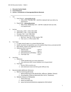

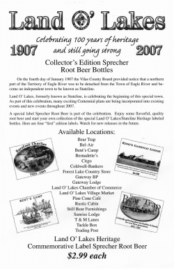
© Copyright 2026